risk theory2.2 risk process (general) what is risk process? safety loading. some classical results...
TRANSCRIPT

University of TartuInstitute of Mathematical Statistics
Risk Theory
Fall 2017
Kalev Parna
Email: [email protected]
1

These notes reflect the content of a course in Risk Theory given at the Instituteof Mathematics and Statistics, UT. The course covers several basic topics relatedto mathematical treatment of risks in financial and actuarial world. The firstmajor topic is ruin theory that analyzes certain random processes which modelthe wealth process of an insurance company. Next we consider basic elementsof portfolio theory, including classical Markowitz model and CAPM model. Thethird main issue is the measurement of financial risk. We focus on Value-at-Risk(VaR) and related methodologies like expected shortfall.
Knowledge of basic concepts and facts of probability theory is a prerequisitefor this course. Some knowledge of stochastic processes, especially Poisson andrenewal processes, is also useful. Still, some more advanced results in these areaswill be given and explained in due course. Basic rules of calculus and some matrixalgebra are also used in this course.
This course is mainly based on following books:
• J. Grandell. Aspects of Risk Theory. Springer-Verlag, 1991.
• A.J. McNeil, R. Frey, P. Embrechts. Quantitative Risk Management: Con-cepts, Techniques and Tools. Princeton University Press, 2005.
• E.J. Elton, M. J. Gruber. Modern Portfolio Theory and Investment Anal-ysis. Wiley, 2003.
2
1 The Concept of Risk
1.1 The meaning of the word
Arabic word risq signifies ”anything that has been given to you [by God] andfrom which you draw profit” and has connotations of a fortuitous (random) andfavorable outcome.
The Latin risicum originally referred to the challenge that a barrier reef presentsto a sailor and has connotations of an equally fortuitous but unfavorable event.
In both cases, the randomness is essential.
Nowadays, English word ”risk” has definite negative associations:
• ”run the risk of ...”
• ” at risk” (= exposed to danger)
Webster’s Dictionary (1981): Risk is ’the possibility of loss, injury, disadvantage,or destruction’
In more specialized literature ’risk’ is also used as a measure of bad outcome. Wecan measure three aspects of a bad outcome:
• the chance (probability) of the bad (negative) outcome,
• its negativity (severity),
• or a combination of both.
Our definition: ”Risk is the possibility of an unfavorable event”
In concrete fields ’risk’ has more specific meaning. In business, the risk oftenmeans chance of loss of money. An investor loses money when the price of thestock or currency he has invested decreases. In insurance business typical riskis possibility of an big claim, or even possibility of the ruin (bankruptcy) of aninsurance company as a result of many big claims that can not be covered by aninsufficient premium flow. The study of ruin probabilities is our first major topicin this course.
Nowadays in almost all fields people face with risks: medicine, industry, ecology,security, defence, sports... It is not possible to avoid risks. The problem is not todecide whether to take the risk or not, but rather which risk to take (should wego from A to B by plane, train, car, or on foot...)
3

Risks are taken by individuals, organizations, and also by governments (e.g. na-tionalization, privatization of big enterprises).
1.2 Risk analysis
‘Analysis is the separation of a whole into its component parts: an examinationof a complex, its elements and their relationships’ (Concise Oxford, 1976).
Purpose of risk analysis: find out all possible outcomes related to the decisionto be made.
The basic risk paradigm:
It is a decision problem in which there is a choice between just two options, one ofwhich will have only one possible outcome (X = no change or status quo), whilstthe other option has two possible outcomes (G = gain, L = loss).
@@@@@
@@@
A
B
x
x
X
G
L
p
1-p
Figure 1: The basic risk paradigm
Examples:
• Investor : to leave money in the bank account (safe option), or to investmoney in a new stock
• Doctor: to prescribe a known drug or to experiment with a new drug
• Advanced example: to marry or not to marry
Practical problems are much more complex, more outcomes (sometimes a contin-uum of possible outcomes), many decisions and processes together. For example,the design of a new chemical plant comprising numerous interconnected processeseach one of which could cause the whole plant to fail.
4
1.3 Risk assessment
The evaluation and comparison of risks is often some form of cost-benefit analysis.It assumes estimation of both probabilities of outcomes and also their severity(magnitudes).
In the basic risk paradigm, when we decide in favor of A, the result will beknown exactly - it is X. If one decides in favor of B, then the expected value ofthe outcome will be
EB(V ) = p G+ (1− p) L.
More generally, when we have more than just two possible outcomes, the expectedvalue will be
EB(V ) =n∑
i=1
pi vi.
The natural idea is to compare EB(V ) with X. If EB(V ) > X then it seems thatwe should take the risk (option B). However, the expected value is not the onlyvalid argument here - in fact, it does not measure the size of the risk. Consideran example to explain this. Suppose G = 1 euro and L = −1 euro with equalprobabilities 0,5 and 0,5 in the basic risk paradigm. Then EB(V ) = 0 and if youtake the risk, you can loose at most 1 euro, which is not a big problem. However,if we replace 1 and -1 by 100 and -100, respectively, then EB(V ) = 0 as before,but now real people are reluctant to choose option B (in order to avoid the bignegative outcome -100). Of course, this is the variance (denoted byDB(V )) whichmakes the difference between these two situations. Hence, also the variance ofthe outcome should be taken into account when deciding between options A andB.
The variance of the outcome is often used as a measure of risk (or even synonymfor ’risk’):
DB(V ) =n∑
i=1
pi (vi − EB(V ))2.
1.4 Risk management
Making practical decisions based on different risk measures.
Well-known financial risk management models:
• risk processes in insurance
• portfolio analysis
5

• value at risk methodologies
• credit scoring
• option pricing.
6

2 Risk processes
2.1 Stochastic processes
Definition 1. Stochastic process (or random process) is a family of randomvariables X(t) : t ∈ T, where t is time parameter and T is the set of possiblevalues of t.
Usually T = 1, 2, ... (discrete time) or T = [0,∞) (continuous time). For eachvalue of t, X(T ) is a random variable.
Counting process is a special case of stochastic processes. Let us consider anevent A that happens from time to time at random time points S1, S2, ... Thenumber of occurrences of the event A within the time interval [0, t] is called acounting process:
N(t) = ♯i : Si ∈ [0, t].
Example: N(t) is the number of claims on the insurance company during thetime interval [0, t].
Let us denote waiting times of the events by
Ti = Si − Si−1.
Definition 2. A counting process N(t) is called Poisson process if its waitingtimes T1, T2, ... are independent random variables having exponential distribution,Ti ∼ Exp(α),∀i. The parameter α is called the intensity of the Poisson process.
Recall that the exponential distribution is defined by its density function
f(x) = α · e−αx, x ≥ 0.
The expected value of an waiting time is
ETi = 1/α.
It is a consequence of the definition above that for any fixed time t, the ran-dom variable N(t) has Poisson distribution with parameter αt , i.e. N(t) ∼Possson(αt), hence its mean (expected) value is
EN(t) = α · t.
It is seen that the higher the density α, the more times the event A happens (inaverage) during the time interval [0, t].
7
2.2 Risk process
(general)
What is risk process? Safety loading. Some classical results in ruin theory
Risk process is a stochastic process for modeling the wealth of an insurance com-pany.
Definition 3. Risk process is a stochastic process defined by
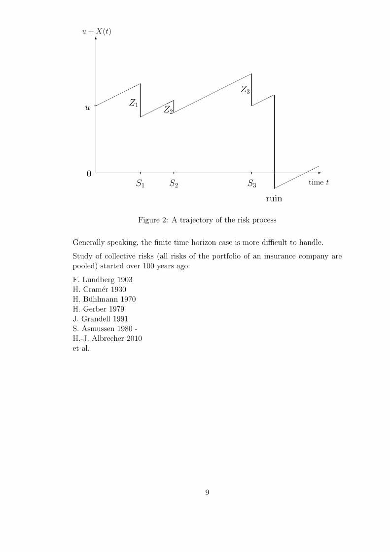
X(t) = ct−N(t)∑k=1
Zk
wherec > 0 - a constant called gross premium rate (the company receives c units ofmoney per unit time),N(t) - the number of claims on the company during (0, t],Zk - the size of claim k.
At each time point S1, S2, ... (the points where N grows) the company has to payout a stochastic amount of money, and the company receives (deterministically)c units of money per unit time.
X(t) is the profit of the company over the time interval (0, t].
Normally an insurance company starts operating with some initial capital u. Min-imum amount of the initial capital is given by regulators.
Ruin of the company means that starting with initial capital u the wealth u+X(t)becomes negative at some time point t.
Ruin probability
Ψ(u) = Pu+X(t) < 0 for some t ∈ (0,∞).
Non-ruin probability: Φ(u) = 1−Ψ(u).
Calculation of the ruin probability is the main task of ruin theory.
In practice, companies are often interested in knowing ruin probability duringnext 4-5 years. For a finite time horizon T the ruin probability is defined by
Ψ(u, T ) = Pu+X(t) < 0 for some t ∈ (0, T ]).
8
0
u
u+X(t)
ruin
Z1Z2
Z3
S1 S2 S3 time t
-
6
Figure 2: A trajectory of the risk process
Generally speaking, the finite time horizon case is more difficult to handle.
Study of collective risks (all risks of the portfolio of an insurance company arepooled) started over 100 years ago:
F. Lundberg 1903H. Cramer 1930H. Buhlmann 1970H. Gerber 1979J. Grandell 1991S. Asmussen 1980 -H.-J. Albrecher 2010et al.
9

2.3 Classical risk process
Here we specify a particularly simple case of risk processes which will be our mainsubject in coming chapters 2-9.
Definition 4. The risk process X(t) = ct −∑N(t)
k=1 Zk is called classical riskprocess if
• Zk∞k=1 are i.i.d. random variables having common distribution functionF (z) with F (0) = 0 and mean value EZk = µ,
• N(t) is a homogenous Poisson process with intensity α and independent ofZk.
NB! We will mainly be interested in this type of risk processes.
Sometimes reversed risk processes are of interest where c < 0 and Zk < 0 (e.g.life annuity)
Let us calculate the expectation of the risk process.
Technical remark 1. (sum of random number of random variables):Let Z1, Z2, ..., ZN be a random number of random variables with EZk = µ. If Nis independent of Zk, then
E(N∑k=1
Zk) = µ · EN.
The proof is elementary (condition on N).
10
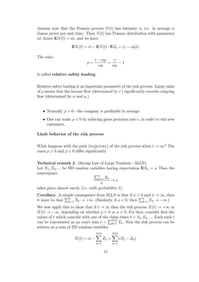
Assume now that the Poisson process N(t) has intensity α, i.e. in average αclaims arrive per unit time. Then N(t) has Poisson distribution with parameterαt, hence EN(t) = αt, and we have
EX(t) = ct− EN(t) · EZk = (c− αµ)t.
The ratio
ρ =c− αµ
αµ=
c
αµ− 1
is called relative safety loading.
Relative safety loading is an important parameter of the risk process. Large valueof ρ means that the income flow (determined by c ) significantly exceeds outgoingflow (determined by α and µ.)
• Normally ρ > 0 - the company is profitable in average.
• One can make ρ < 0 by reducing gross premium rate c, in order to win newcustomers.
Limit behavior of the risk process
What happens with the path (trajectory) of the risk process when t → ∞? Thecases ρ > 0 and ρ < 0 differ significantly.
Technical remark 2. (Strong Law of Large Numbers - SLLN)Let X1, X2, ... be IID random variables having expectation EXk = a Then theconvergence ∑n
k=1Xk
n→ a
takes place almost surely (i.e. with probability 1).
Corollary. A simple consequence from SLLN is that if a > 0 and n → ∞, thenit must be that
∑nk=1Xk → +∞. (Similarly, if a < 0, then
∑nk=1Xk → −∞.)
We now apply this to show that if t → ∞ then the risk process X(t) → +∞ orX(t) → −∞, depending on whether ρ > 0 or ρ < 0. For that, consider first thevalues of t which coincide with one of the claim times t = S1, S2, .... Each such tcan be represented as an exact sum t =
∑N(t)k=1 Tk. Now the risk process can be
written as a sum of IID random variables
X(t) = ct−N(t)∑k=1
Zk =
N(t)∑k=1
(cTk − Zk).
11
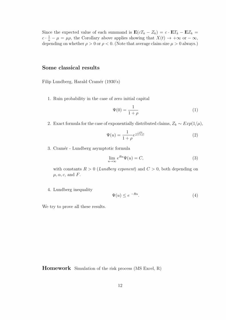
Since the expected value of each summand is E(cTk − Zk) = c · ETk − EZk =c · 1
α− µ = µρ, the Corollary above applies showing that X(t) → +∞ or − ∞,
depending on whether ρ > 0 or ρ < 0. (Note that average claim size µ > 0 always.)
Some classical results
Filip Lundberg, Harald Cramer (1930’s)
1. Ruin probability in the case of zero initial capital
Ψ(0) =1
1 + ρ(1)
2. Exact formula for the case of exponentially distributed claims, Zk ∼ Exp(1/µ),
Ψ(u) =1
1 + ρe
−ρuµ(1+ρ) (2)
3. Cramer - Lundberg asymptotic formula
limu→∞
eRuΨ(u) = C, (3)
with constants R > 0 (Lundberg exponent) and C > 0, both depending onµ, α, c, and F .
4. Lundberg inequalityΨ(u) ≤ e −Ru. (4)
We try to prove all these results.
Homework Simulation of the risk process (MS Excel, R)
12
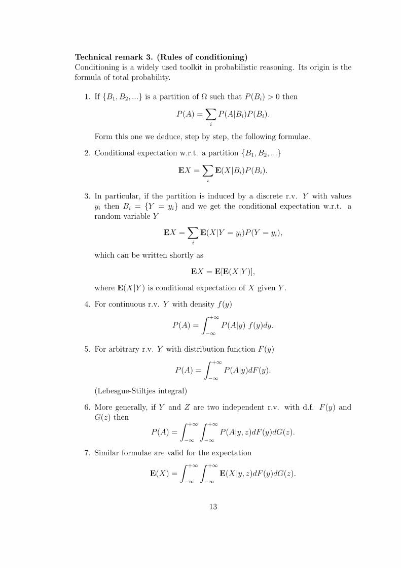
Technical remark 3. (Rules of conditioning)Conditioning is a widely used toolkit in probabilistic reasoning. Its origin is theformula of total probability.
1. If B1, B2, ... is a partition of Ω such that P (Bi) > 0 then
P (A) =∑i
P (A|Bi)P (Bi).
Form this one we deduce, step by step, the following formulae.
2. Conditional expectation w.r.t. a partition B1, B2, ...
EX =∑i
E(X|Bi)P (Bi).
3. In particular, if the partition is induced by a discrete r.v. Y with valuesyi then Bi = Y = yi and we get the conditional expectation w.r.t. arandom variable Y
EX =∑i
E(X|Y = yi)P (Y = yi),
which can be written shortly as
EX = E[E(X|Y )],
where E(X|Y ) is conditional expectation of X given Y .
4. For continuous r.v. Y with density f(y)
P (A) =
∫ +∞
−∞P (A|y) f(y)dy.
5. For arbitrary r.v. Y with distribution function F (y)
P (A) =
∫ +∞
−∞P (A|y)dF (y).
(Lebesgue-Stiltjes integral)
6. More generally, if Y and Z are two independent r.v. with d.f. F (y) andG(z) then
P (A) =
∫ +∞
−∞
∫ +∞
−∞P (A|y, z)dF (y)dG(z).
7. Similar formulae are valid for the expectation
E(X) =
∫ +∞
−∞
∫ +∞
−∞E(X|y, z)dF (y)dG(z).
13

3 Derivation of integral equation for ruin prob-
ability
We show here that the non-ruin probability Φ(u) satisfies an integral equation.To derive the equation, we will use the rule of conditioning, combined with a”renewal” argument.
We condition upon S1 and Z1 - the time and the size of the first claim (see therule 6. of conditioning w.r.t. two random variables where A means ’non-ruin’).Suppose S1 and Z1 take values S1 = s and Z1 = z and calculate the conditionalnon-ruin probability P (A|s, z) needed in rule 6. First note that at time S1 therisk process equals u + X(S1) = u + cs − z. However, at time S1 = s the riskprocess starts anew, with the only difference that, instead of u, the initial capitalis u + cs − z. Since ruin can not occur before time S1, the conditional non-ruinprobability is the same as the non-ruin probability with this new initial capital:P (A|s, z) = Φ(u+ cs− z). Integrating over all possible values of S1 and Z1, onehas:
Φ(u) =
∫ ∞
0
∫ ∞
0
Φ(u+ cs− z)dFS1(s)dF (z),
where FS1(s) and F (z) are distribution functions of S1 and Z1, respectively.
Since the distribution of S1 is exponential, we can replace dFS1(s) = αe−αsds,
and since a large first claim z ≥ u+ cs imply immediate ruin, we can restrict thedomain of integration
Φ(u) =
∫ ∞
s=0
αe−αs
∫ u+cs
z=0
Φ(u+ cs− z)dF (z)ds.
The change of variables x = u+ cs⇒ ds = dx/c leads to
Φ(u) =α
ceαu/c
∫ ∞
u
αe−αx/c
∫ x
0
Φ(x− z)dF (z)dx.
Consiquently Φ is differentiable and differentation (using (fg)′ = f ′g + fg′ and[∫ u
0f(x)dx]′ = f(u)) leads to
Φ′(u) =α
c· αceαu/c
∫ ∞
u
αe−αx/c
∫ x
0
Φ(x− z)dF (z)dx
− α
ceαu/c · e−αu/c
∫ u
0
Φ(u− z)dF (z).
The first term on the right hand side equals αcΦ(u) and hence we have
14

Φ′(u) =α
cΦ(u)− α
c
∫ u
0
Φ(u− z)dF (z). (5)
Replacing dF (z) = −d(1−F (z)) and integrating by parts (∫fdg = fg| −
∫gdf)
we have
Φ′(u) =α
cΦ(u) +
α
c
∫ u
0
Φ(u− z)d(1− F (z))
=α
cΦ(u) +
α
c[Φ(0)(1− F (u))− Φ(u)] +
α
c
∫ u
0
Φ′(u− z)(1− F (z))dz
=α
cΦ(0)(1− F (u)) +
α
c
∫ u
0
Φ′(u− z)(1− F (z))dz
Integrating over (0, t) yields
Φ(t)− Φ(0) = =α
cΦ(0)
∫ t
0
(1− F (u))du+α
c
∫ t
0
∫ u
0
Φ′(u− z)(1− F (z))dzdu
(now change the order of integration in the double integral)
=α
cΦ(0)
∫ t
0
(1− F (u))du+α
c
∫ t
z=0
(1− F (z))
∫ t
u=z
Φ′(u− z)dudz
=α
cΦ(0)
∫ t
0
(1− F (u))du+α
c
∫ t
z=0
(1− F (z))[Φ(t− z)− Φ(0)]dz
=α
c
∫ t
0
(1− F (z))Φ(t− z)dz
Thus we can write
Φ(u) = Φ(0) +α
c
∫ u
0
Φ(u− z)[1− F (z)]dz. (6)
This is an integral equation since the unknown function Φ(u) stands under theintegral sign. We will see that this equation can be used for several purposes.
15

4 Ruin probability with 0 capital
We assume that ρ > 0 i.e. the company is profitable. If the initial capital u iszero, the ruin probability takes very simple form (see the ’classical’ result (1)).To show that, we first recall a result from integration theory indicating when itis possible to exchange the order of integration and limiting process.
Technical remark (Monotone Convergence Theorem)Let 0 ≤ fn(x) ↑ and let fn(x) be integrable, ∀n = 1, 2, .... Then there ex-ists an integrable limit function f(x) = limn fn(x) and the equality
∫f(x)dx =
limn
∫fn(x)dx holds.
By monotone convergence it follows from (6), as u→ ∞, that
Φ(∞) = Φ(0) +α µ
cΦ(∞). (7)
Show that Φ(∞) = 1. It suffices to show that for ρ > 0 the process X(t) neverattains the value −∞, remaining always finite (then u +X(t) > 0,∀t and therewill not be ruin). First recall that for ρ > 0 the paths of the risk process tendto infinity, limt→∞X(t) = +∞ a.s. It follows that there exists time T = T (ω)such that for all t > T we have X(t) > 0. Hence there cannot be ruin afterthe time T. On the other side, before the time T (i.e. within the interval [0, T ])only a finite number of claims arrive a.s. (since N(T ) has Poisson distribution).Therefore, since each claim has finite size, the total sum to be payed out within[0, T ] is finite. Hence, with infinite initial capital, the process cannot ruin beforethe time T either. To conclude, the non-ruin probability Φ(∞) = 1. By insertingthis into (7) we get
1 = Φ(0) +α µ
c,
which, together with the definition of ρ, gives the classical result (1):
Ψ(0) =1
1 + ρwhen c > αµ.
16

5 Exponentially distributed claims
Consider the case when the claims are exponentially distributed, Zk ∼ Exp(1/µ).Our aim is to prove the classical result (2):
Ψ(u) =1
1 + ρe
−ρuµ(1+ρ)
The starting point is the following equation, obtained in Section 3:
Φ′(u) =α
cΦ(u)− α
c
∫ u
0
Φ(u− z)dF (z).
Since the claims’ distribution F is exponential with mean value µ, we can replacedF (z) = 1
µe−z/µdz to obtain
Φ′(u) =α
cΦ(u)− α
cµ
∫ u
0
Φ(u− z)e−z/µdz.
Change of variables u− z =: v, dz = −dv gives (using −∫ 0
u... =
∫ u
0...)
Φ′(u) =α
cΦ(u)− α
cµ
∫ u
0
Φ(z)e−(u−z)/µdz,
or
Φ′(u) =α
cΦ(u)− α
cµe−u/µ
∫ u
0
Φ(z)ez/µdz.
Differentiation by u (using rules (fg)′ = f ′g+fg′ and (∫ u
ah(x)dx)
′u = h(u)) leads
to
Φ′′(u) =α
cΦ′(u) +
1
µ
(αcΦ(u)− Φ′(u)
)− α
cµΦ(u)
= (α
c− 1
µ)Φ′(u) = − ρ
µ(1 + ρ)Φ′(u).
From here we have (lnΦ′(u))′ = Φ′′(u)Φ′(u)
= − ρµ(1+ρ)
, and , hence,
lnΦ′(u) = − ρu
µ(1 + ρ)+ C1
from which
Φ′(u) = C2e− ρu
µ(1+ρ) ⇒ Φ(u) = C3e− ρu
µ(1+ρ) + C4.
17

The constants C3 and C4 are defined by conditions Φ(∞) = 1 (giving C4 = 1)and Φ(0) = 1− 1/(1 + ρ) (giving C3 = −1/(1 + ρ). Therefore,
Φ(u) = 1− 1
1 + ρe−
ρuµ(1+ρ)
which is equivalent to the classical result (2).
Exercise. An insurance company is earning EUR 13200 per day (netto). Itreceives in average 20 claims per day with average claim size of EUR 600. Findthe relative safety loading. Assuming that the claims sizes are exponentiallydistributed, calculate the ruin probability of the company at the time momentwhen its wealth is equal to EUR 25 000. Find the wealth of the company suchthat the probability of possible ruin in the future is less than 0,01%.
18

6 Cramer-Lundberg approximation to the ruin
probability
Our aim here is to show the classical result (3), called Cramer-Lundberg approx-imation. We assume that ρ > 0, or c > αµ. The starting point is the equation(6):
Φ(u) = Φ(0) +α
c
∫ u
0
Φ(u− z)[1− F (z)]dz.
Form this and from classical result (1) we get the following:
1−Ψ(u) = 1− αµ
c+α
c
∫ u
0
(1−Ψ(u− z))[1− F (z)]dz
= 1− α
c
(µ−
∫ u
0
[1− F (z)]dz +
∫ u
0
Ψ(u− z)[1− F (z)]dz
)or , by using µ =
∫∞0[1− F (x)]dx,
Ψ(u) =α
c
∫ ∞
u
[1− F (z)]dz +α
c
∫ u
0
Ψ(u− z)[1− F (z)]dz. (8)
To solve for Ψ(u) this ’renewal type’ equation, we rely on the following.
Technical remark (Key renewal theorem)Let G(u) satisfy the following (’renewal type’) equation:
G(u) = H(u) +
∫ u
0
G(u− x)dA(x), (9)
where H is known, A is a given distribution function. Then the asymptoticsolution is given by:
limu→∞
G(u) = limu→∞
H(u) +1
µA
∫ ∞
0
H(u)du, (10)
where µA is the expectation of the distribution A, 0 < µA <∞.
However, since∫∞0
αc[1 − F (z)]dz = αµ
c< 1, equation (8) is not directly of type
(9) (for the function αc[1 − F (z)] to be regarded as a density of a distribution
A, this integral must be equal to 1.) W. Feller overcame the difficulty by mul-tiplying both sides of the equation (8) by eRu, where R > 0 is properly chosenconstant(Lundberg exponent). We therefore assume that there exists a constantR > 0 such that
α
c
∫ ∞
0
eRz[1− F (z)]dz = 1. (11)
19

Then αceRz[1−F (z)] is the density of a proper density distribution. Multiplication
of (8) by eRu yields
eRuΨ(u) =α
ceRu
∫ ∞
u
(1− F (z))dz +α
c
∫ u
0
eR(u−z)Ψ(u− z)eRz[1− F (z)]dz.
which is a proper renewal equation. From the key renewal theorem it then followsthat
limu→∞
eRuΨ(u) =C1
C2
, (12)
where
C1 =α
c
∫ ∞
0
eRu
∫ ∞
u
(1− F (z))dzdu (13)
and
C2 =α
c
∫ ∞
0
zeRz(1− F (z))dz (14)
provided that finite positive numbers R,C1, C2 exist.
(How the functions G(u), H(u) and A(x) should be specified when applying theKey renewal theorem?)
Let us now calculate C1 and C2.
Calculation of C1. Change of the order of integration in (13) gives
C1 =α
c
∫ ∞
0
(1− F (z)
∫ z
0
eRududz.
Since∫ z
0eRudu = 1
ReRz − 1
Rone obtains
C1 =α
Rc
∫ ∞
0
eRz(1− F (z))dz − α
Rc
∫ ∞
0
(1− F (z))dz =1
R− αµ
Rc=
1
R· ρ
1 + ρ.
(Here we used relationships (11) and∫∞0(1− F (z))dz = µ.)
20
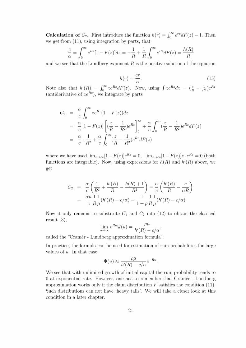
Calculation of C2. First introduce the function h(r) =∫∞0erzdF (z)− 1. Then
we get from (11), using integration by parts, that
c
α=
∫ ∞
0
eRz[1− F (z)]dz = − 1
R+
1
R
∫ ∞
0
eRzdF (z) =h(R)
R
and we see that the Lundberg exponent R is the positive solution of the equation
h(r) =cr
α. (15)
Note also that h′(R) =∫∞0zeRzdF (z). Now, using
∫zeRzdz = ( z
R− 1
R2 )eRz
(antiderivative of zeRz), we integrate by parts
C2 =α
c
∫ ∞
0
zeRz(1− F (z))dz
=α
c[1− F (z)]
[(z
R− 1
R2)eRz
]∞0
+α
c
∫ ∞
0
(z
R− 1
R2)eRzdF (z)
=α
c· 1
R2+α
c
∫ ∞
0
(z
R− 1
R2)eRzdF (z)
where we have used limz→∞[1−F (z)]eRz = 0, limz→∞[1−F (z)]z · eRz = 0 (bothfunctions are integrable). Now, using expressions for h(R) and h′(R) above, weget
C2 =α
c
(1
R2+h′(R)
R− h(R) + 1
R2
)=α
c
(h′(R)
R− c
αR
)=
αµ
c
1
R
1
µ(h′(R)− c/α) =
1
1 + ρ
1
R
1
µ(h′(R)− c/α).
Now it only remains to substitute C1 and C2 into (12) to obtain the classicalresult (3),
limu→∞
eRuΨ(u) =ρµ
h′(R)− c/α,
called the ”Cramer - Lundberg approximation formula”.
In practice, the formula can be used for estimation of ruin probabilities for largevalues of u. In that case,
Ψ(u) ≈ ρµ
h′(R)− c/αe−Ru.
We see that with unlimited growth of initial capital the ruin probability tends to0 at exponential rate. However, one has to remember that Cramer - Lundbergapproximation works only if the claim distribution F satisfies the condition (11).Such distributions can not have ’heavy tails’. We will take a closer look at thiscondition in a later chapter.
21

Exercise
Find the Lundberg constant R for the case when all claim sizes are equal to 1(such claims can be interpreted as winnings in a lottery with fixed prizes).
ExerciseCramer-Lundberg approximation is precise in the case of exponentially distributedclaims.
Suppose that the claims are exponentially distributed with mean µ , Zi ∼ Exp(1/µ).Prove that then the Cramer-Lundberg approximation is exact.
Hints:1) show that h(r) = µr
1−µr
2) show that the Lundberg exponent satisfies R = ρµ(1+ρ)
3) calculate h′(R) = µ(1 + ρ)2
4) show that the right-hand term of Cramer-Lundberg formula verifies
ρµ
h′(R)− c/α)=
1
1 + ρ
5) Compare the result with the classical result (2). (Comment!)
22

7 Lundberg exponent
The Lundberg exponent was defined by (11) as a positive number R > 0 suchthat
α
c
∫ ∞
0
eRz[1− F (z)]dz = 1. (16)
From this it follows that eRz[1−F (z)] → 0 as z → ∞. Therefore, 1−F (z) musttend to 0 faster than e−Rz, i.e. the tail of F must be light. A simple positive exam-ple here is the exponential distribution. (In fact, our Homework showed that forexponentially distributed claims the Lundberg exponent equals R = ρ/µ(1 + ρ).However, we now show that many standard distributions do not satisfy this con-dition, e.g. Pareto, lognormal, or Weibull with shape parameter smaller than 1.
Three examples of heavy-tailed claim distributions
Example 1. The Pareto density is
f(z) = αβα
zα+1, z > β, α > 0.
The tail of the Pareto distribution is 1 − F (z) =(βz
)α, which decreases with
power speed, i.e. too slowly, since
eRz[1− F (z)] = eRz
(β
z
)α
→ ∞ for any R > 0.
Hence, for the Pareto distribution the Lundberg exponent does not exist. Notethat Pareto distribution is generally accepted as a good model for claim sizes infire insurance.
Example 2. By definition, Z has log-normal distribution, Z ∼ LN(µ, σ), iflnZ ∼ N(µ, σ). The log-normal density is
f(z) =1
z√2πσ
exp
−(ln z − µ)2
2σ2
.
Let for simplicity µ = 0, σ = 1. Then lnZ ∼ N(0, 1) and the distribution functionof Z is obtained as
F (z) = P (Z < z) = P (lnZ < ln z) = Φ(ln z),
where Φ(·) is the distribution function of N(0, 1). Since for large z, 1 − Φ(z) ∼1zφ(z), the tail
1− F (z) = 1− Φ(ln z) ∼ 1
ln zφ(ln z) =
1
ln z√2πe−
(ln z)2
2 .
23

Therefore
eRz[1− F (z)] ∼ 1
ln z√2πeRz− (ln z)2
2 >1
ln z√2πeRz/2
for z large enough. However, the latter tends to ∞ for any R > 0, when z → ∞.Hence, for the log-normal distribution the Lundberg exponent does not exist.Note that log-normal distribution is generally accepted as a good model for claimsizes in motor insurance.
Example 3. The Weibull distribution is defined by its density
f(z) =γzγ−1
βγexp
[−(z
β
)γ], 0 ≤ z <∞, β > 0, γ > 0.
Note that the case of γ = 1 reduces to the exponential distribution. The tail ofthe Weibull distribution is
1− F (z) = exp
[−(z
β
)γ].
ThereforeeRz[1− F (z)] = eRze−(z/β)γ = eRz−(z/β)γ ,
which goes to +∞ for γ < 1 and −∞ for γ ≥ 1. Hence, the Lundberg exponentexists only for γ ≥ 1.
24
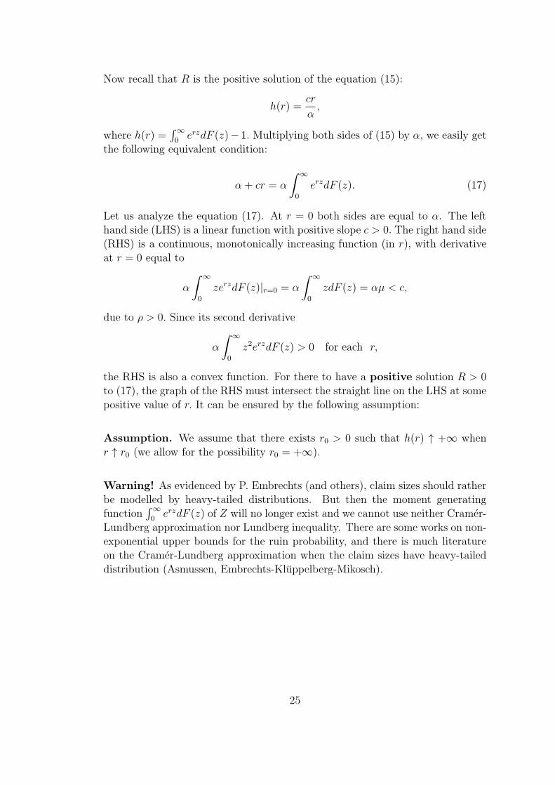
Now recall that R is the positive solution of the equation (15):
h(r) =cr
α,
where h(r) =∫∞0erzdF (z)− 1. Multiplying both sides of (15) by α, we easily get
the following equivalent condition:
α + cr = α
∫ ∞
0
erzdF (z). (17)
Let us analyze the equation (17). At r = 0 both sides are equal to α. The lefthand side (LHS) is a linear function with positive slope c > 0. The right hand side(RHS) is a continuous, monotonically increasing function (in r), with derivativeat r = 0 equal to
α
∫ ∞
0
zerzdF (z)|r=0 = α
∫ ∞
0
zdF (z) = αµ < c,
due to ρ > 0. Since its second derivative
α
∫ ∞
0
z2erzdF (z) > 0 for each r,
the RHS is also a convex function. For there to have a positive solution R > 0to (17), the graph of the RHS must intersect the straight line on the LHS at somepositive value of r. It can be ensured by the following assumption:
Assumption. We assume that there exists r0 > 0 such that h(r) ↑ +∞ whenr ↑ r0 (we allow for the possibility r0 = +∞).
Warning! As evidenced by P. Embrechts (and others), claim sizes should ratherbe modelled by heavy-tailed distributions. But then the moment generatingfunction
∫∞0erzdF (z) of Z will no longer exist and we cannot use neither Cramer-
Lundberg approximation nor Lundberg inequality. There are some works on non-exponential upper bounds for the ruin probability, and there is much literatureon the Cramer-Lundberg approximation when the claim sizes have heavy-taileddistribution (Asmussen, Embrechts-Kluppelberg-Mikosch).
25

8 Short overview of heavy-tailed distributions
As it has been mentioned above in several cases, good models for claim distribu-tions encompasse heavy tails.
Heavy-tailed distributions are probability distributions whose tails are not expo-nentially bounded: that is, they have heavier tails than the exponential distribu-tion. In many applications it is the right tail of the distribution that is of interest,but a distribution may have a heavy left tail, or both tails may be heavy.
There are three important subclasses of heavy-tailed distributions,
• the fat-tailed distributions,
• the long-tailed distributions,
• the subexponential distributions.
In practice, all commonly used heavy-tailed distributions belong to the subexpo-nential class.
There is still some discrepancy over the use of the term heavy-tailed. There aretwo other definitions in use. However, the definition given below is the mostgeneral in use, and includes all distributions encompassed by the alternative def-initions (e.g. log-normal that possess all their power moments, yet which aregenerally acknowledged to be heavy-tailed.)
Definition of heavy-tailed distribution
The distribution of a random variable X with distribution function F is said tohave a heavy right tail if
limx→∞
eλx Pr[X > x] = ∞ for all λ > 0.
This is also written in terms of the tail distribution function
F (x) ≡ Pr[X > x]
as
limx→∞
eλxF (x) = ∞ for all λ > 0.
This is equivalent to the statement that the moment generating function of F ,MF (t) = E(etX), is infinite for all t > 0.
The definitions of heavy-tailed for left-tailed or two tailed distributions are simi-lar.
26

Definition of fat-tailed distribution
The distribution of a random variable X is said to have a fat tail if
Pr[X > x] ∼ x−α as x→ ∞, α > 0.
That is, if X has a probability density function, fX(x),
fX(x) ∼ x−(1+α) as x→ ∞, α > 0.
Here the notation ” ∼” means the asymptotic equivalence of functions. Somereserve the term ”fat tail” for distributions only where 0 < α < 2 (i.e. only incases with infinite variance).
Definition of long-tailed distribution
The distribution of a random variable X with distribution function F is said tohave a long right tail if for all t > 0,
limx→∞
Pr[X > x+ t|X > x] = 1,
or equivalently
F (x+ t) ∼ F (x) as x→ ∞.
This has the intuitive interpretation for a right-tailed long-tailed distributed quan-tity that if the long-tailed quantity exceeds some high level, the probability ap-proaches 1 that it will exceed any other higher level: if you know the situation isbad, it is probably worse than you think.
All long-tailed distributions are heavy-tailed, but the converse is false, and it ispossible to construct heavy-tailed distributions that are not long-tailed.
The class of long-tailed distributions is often denoted by L.
Subexponential distributions
Subexponentiality is defined in terms of convolutions of probability distributions.For two independent, identically distributed random variables X1, X2 with com-mon distribution function F the convolution of F with itself, F ∗2 is defined, usingLebesgue–Stieltjes integration, by:
Pr[X1 +X2 ≤ x] = F ∗2(x) =
∫ ∞
−∞F (x− y) dF (y)
.
The n-fold convolution F ∗n is defined in the same way. The tail distributionfunction F is defined as F (x) = 1− F (x).
27

A distribution F on the positive half-line is subexponential if
F ∗2(x) ∼ 2F (x) as x→ ∞.
This implies that, for any n ≥ 1,
F ∗n(x) ∼ nF (x) as x→ ∞. (18)
This condition has a rather simple interpretation. Note that nF (x) is the tail ofthe distribution of the maxima of n random variables X1, · · · , Xn. Indeed, dueto (1− a)n ∼ 1− na when a→ 0, we have
Pr[max(X1, . . . , Xn) > x] = 1− F n(x) = 1− (1− F (x))n ∼ nF (x) (19)
Therefore, the probabilistic interpretation of (18) is that, for a sum of n indepen-dent random variables X1, . . . , Xn with common distribution F ,
Pr[X1 + · · ·+Xn > x] ∼ Pr[max(X1, . . . , Xn) > x] as x→ ∞.
This is often known as the principle of the single big jump.
The class of subexponential distributions is often denoted by S.
All subexponential distributions are long-tailed, but examples can be constructedof long-tailed distributions that are not subexponential.
Common heavy-tailed distributions
All commonly used heavy-tailed distributions are subexponential.
Those that are one-tailed include:
• the Pareto distribution;
• the Log-normal distribution;
• the Levy distribution;
• the Weibull distribution with shape parameter less than 1;
• the Burr distribution;
• the log-gamma distribution;
• the log-Cauchy distribution, sometimes described as having a ”super-heavytail” because it exhibits logarithmic decay producing a heavier tail than thePareto distribution.
28

Those that are two-tailed include:
• The Cauchy distribution, itself a special case of both the stable distributionand the t-distribution;
• The family of stable distributions, excepting the special case of the normaldistribution within that family. Some stable distributions are one-sided (orsupported by a half-line), see e.g. Levy distribution. See also financialmodels with long-tailed distributions and volatility clustering.
• The t-distribution.
• The skew lognormal cascade distribution.
References
1. Asmussen, S. (2003). Applied Probability and Queues. Berlin: Springer.
2. Rolski, Schmidli, Scmidt, Teugels, Stochastic Processes for Insurance andFinance, 1999
3. Embrechts, P., Kluppelberg, C., Mikosch, T. (1997). Modelling ExtremalEvents for Insurance and Finance. Berlin: Springer.
29

9 Lundberg inequality
The Lundberg exponent plays an important role in the ruin theory. We nextshow the classical result (4).
Theorem 1. (Lundberg inequality) For the classical risk process the proba-bility of ruin Ψ(u) satisfies
Ψ(u) ≤ e−Ru,−∞ < u <∞, (20)
where R > 0 is the Lundberg exponent.
Proof. Let A be the event that starting with the initial capital u the risk processwill ruin. Then Ψ(u) = P (A). Let us denote
An = the ruin occurs as a result of first n claims, n = 1, 2, ...
andA0 = the ruin occurs as a result of a negative initial capital.
Let the corresponding probabilities be Ψn(u) = P (An). Obviously, it is an in-creasing sequence of events: An ⊂ An+1, n = 0, 1, 2, .... Further on, as the ruinmeans that at least one of the events An occurs, then A = ∪nAn. By the conti-nuity of probability we have P (A) = limP (An), or Ψ(u) = limΨn(u). Therefore,it suffices to show that for each n ≥ 0 the inequality
Ψn(u) ≤ e−Ru (21)
holds. For doing that, we use the method of mathematical induction. Show firstthat the inequality holds for n = 0 (induction basis). Since Ψ0(u) = 1 for u < 0(negative initial capital means the ruin) and Ψ0(u) = 0 for u ≥ 0, the inequalityΨ0(u) ≤ e−Ru holds, as far as R > 0.
Show now that if the inequality (21) holds for an n − 1, then it also holds forn. To do that, we condition upon S1 and Z1, the time and the size of the firstclaim. If the first claim arrived at time S1 = s and its size was Z1 = z, thenafter paying out the first claim, the company’s capital is u + cs − z. Startingwith this new capital at time S1 = s, the event An defined above is equivalentto the ruin due to next ≤ n− 1 claims, and therefore the conditional probabilityP (An|S1 = s, Z1 = z) = Ψn−1(u+ cs−z). According to the rules of conditioning,we now average (integrate) such conditional probabilities over all possible valuesof S1 and Z1, while keeping in mind that S1 has exponential distribution, S1 ∼Exp(α), and that Z1 has distribution F :
Ψn(u) = P (An) =
∫ ∞
0
∫ ∞
0
P (An|S1 = s, Z1 = z)fS1(s)dF (z)ds.
30

As the exponential density is fS1(s) = αe−αs, s ≥ 0, we have, after substitution,that
Ψn(u) =
∫ ∞
0
αe−αs
∫ ∞
0
Ψn−1(u+ cs− z)dF (z)ds.
As we assume that Ψn−1(u) satisfies (21), we have Ψn−1(u+ cs−z) ≤ e−R(u+cs−z)
which gives
Ψn(u) ≤∫ ∞
0
αe−αs
∫ ∞
0
e−R(u+cs−z)dF (z)ds = e−Ru·α∫ ∞
0
e−(α+Rc)sds·∫ ∞
0
eRzdF (z).
Direct integration shows that∫ ∞
0
e−(α+Rc)sds =1
α+Rc
(here it is necessary to take into account that α + Rc > 0), which gives theinequality
Ψn(u) ≤ e−Ru · α
α +Rc
∫ ∞
0
eRzdF (z).
However, by the definition of the Lundberg exponent R, the second multipliersatisfies α
α+Rc
∫∞0eRzdF (z) = 1, therefore we have shown that
Ψn(u) ≤ e−Ru.
The proof is completed.
In order to use the Lundberg inequality, it would be good to have bounds for theLundberg exponent R.
Derivation of a lower bound for R.
Suppose that the claims are bounded above by some constant K, i.e. Z ≤ K.Then for z ≤ K the inequality
eRz ≤ z
KeRK + (1− z
K). (22)
holds. Indeed, due to the well-known expansion formula
ez = 1 + z +z2
2!+z3
3!+ . . . ,
we have
z
KeRK + (1− z
K) = 1− z
K+
z
K+
z
KRK +
z
K
R2K2
2!+
z
K
R3K3
3!+ . . .
≥ 1 + zR +R2z2
2!+ . . .
= eRz.
31

Now recall the equation (17) which defines R, and apply (22):
α + cR = α
∫ ∞
0
eRzdF (z) = αE(eRZ)
≤ α( µKeRK + 1− µ
K
).
From this we have:
cR ≤ αµ
K(eRK − 1),
or
eRK − 1
KR≥ c
αµ≡ 1 + ρ.
Now a small ’trick’ i.e. the inequality ex−1x
< ex can be used to obtain
eRK ≥ 1 + ρ,
which gives
R >1
Kln(1 + ρ).
Corollary. If the claims are bounded, Z ≤ K, then the ruin probability satisfies
Ψ(u) ≤ (1 + ρ)−u/K . (23)
Example
An insurance company is running business under following conditions:- it earns in average EUR 50 000 per day from selling insurance policies ,- it receives in average 10 claims per day,- the average claim is EUR 4 000.- the claim size is bounded from above by EUR 100 000.1) Assuming that all conditions of the classical risk process are fulfilled, estimatethe ruin probability for initial capitals EUR 10k, 100k, 1m, 5m, and 10m, usingthe Lundberg inequality.2) Draw a graph of the upper bound of the ruin probability (with initial capitalon the x-axis.)
32

10 Simple approximations of ruin probabilities
It is natural to try to find “simple” and “good” approximations of Ψ(u).
A “simple approximation” of a ruin probability is an approximation using onlysome moments of the claim distribution and not the detailed tail behaviour ofthat distribution. Such approximations may be based on more or less ad hocarguments and their merits can only be judged by numerical comparison. Othersare based on limit theorems, and the limit procedure may give hints on theirapplicability. In that case numerical comparison may be needed in order to getinformation about the speed of convergence and — which is almost the same —their numerical accuracy.
The most successful simple approximation is certainly the De Vylder approxima-tion, which is based on the idea to replace the risk process with a risk processwith exponentially distributed claims such that the three first moments coincide.That approximation is known to work extremely well for “kind” claim distribu-tions. The purpose of this chapter is to analyse the De Vylder approximationand other simple approximations from a more mathematical point of view.
Several such approximations have been proposed. The most famous approxima-tion is, of course, the Cramer–Lundberg approximation (3):
limu→∞
eRuΨ(u) =ρµ
h′(R)− c/α.
This approximation, which goes back to Cramer (1930), works well in case of lighttail claim distributions, and is very accurate for large values of u. The approxi-mation requires that the tail of F decreases at least exponentially fast, and thusfor instance the lognormal and the Pareto distributions are excluded. In order toinclude that last mentioned distributions it is usual to consider distributions Fsuch that its itd FI belongs to the class S of subexponential distribution. Then,as we have seen already,
ψ(u) ∼ FI(u)
ρ, u→ ∞,
does hold exactly. However, the latter approximation has a much slower speed ofconvergence than that of Cramer–Lundberg ( see e.g. Grandell (1997, p. 222).
Both approximations above are practically somewhat difficult to apply, since theyrequire full knowledge of the claim distribution. Notice that they apply for fixedvalues of ρ as u→ ∞. Thus those approximations may be looked upon as “largedeviation” results and it is seen that the asymptotic behaviour of Ψ(u) is verydifferent.
We will concentrate on “simple” approximations, by which we mean that theapproximations only depend on some moments of F. The simplest such approxi-
33
mation seems to be the diffusion approximation:
Ψ(u) ≈ ΨD(u) := e−uρ
2ζ1ζ2 .
whereζk = E(Zk
1 )
are the moments of the claim size distribution F . (Note that ζ1 = µ.) This ap-proxiamtion goes back to Hadwiger (1940). It is nowadays derived by applicationof weak convergence of the compound Poisson process to a Wiener process, seefor instance Grandell (1991). It may be used if ρ is small and u is large in sucha way that u and ρ−1 are of the same order. In queuing theory is known as the“heavy traffic approximation”. The numerical accuracy of this approximation isnot very impressive. It is natural to regard the asymptotic behind the diffusionapproximation as a “central limit” situation in the sense that many claims “co-operate” on almost equal terms. It seems that simple approximations can onlybe expected to work well in such a case. Similarly as one shall apply the centrallimit theorem with great care far out in the tails, one may suspect that simpleapproximations ought to be used mainly when the ruin probability is not toosmall.
De Vylder approximation
The De Vylder approximation, proposed by De Vylder (1978), is based on thesimple, but ingenious, idea to replace the risk process X with a risk process Xwith exponentially distributed claims such that
E[Xk(t)] = E[Xk(t)] for k = 1, 2, 3.
The risk process X is determined by the three parameters (α, c, µ) or (α, ρ, µ).
We can calculate the three first moments (using characteristic function of X(t) ,for example):
E[Xt)] = (c− αµ)t = ραζ1t, (as we already know)
E[X2(t)] = αζ2t+ (ραζ1t)2,
E[X3(t)] = −αζ3 + 3(ραζ1t)(αζ2t) + (ραζ1t)3.
Respective moments of the process X(t) can also be calculated:
34
By equating the moments of the two processes we see that the parameters (α, ρ, µ)must satisfy
ραζ1t = ραµ, αζ2 = 2αµ2, αζ3 = 6αµ3,
and we get
µ =ζ33ζ2
, ρ =2ζ1ζ33ζ22
ρ.
Thus we are led to the De Vylder’s approximation
Ψ(u) ≈ ΨDV (u) :=1
1 + ρe−
ρuµ(1+ρ) .
Many other approximations have been introduced. However, the De Vylder’sapproximation is considered as very simple and very often surprisingly precise.
35
11 Further generalizations of the classical risk
processes
The classical risk process studied in the previous sections is a simplified modelof the wealth of an insurance company. Next some possible extensions are shownthat introduce more realistic features into the model.
A. The premiums may depend on the result of the insurance business. Forexample, it is natural to make the safety loading smaller if the risk businessattains a large value.
B. Inflation and interest may be included in the model.
C. The claim arrival process may be described by a more general process thanthe Poisson process:
1. Non-homogeneous Poisson processes
2. Cox processes
3. Renewal processes
The classical result (1) remains valid for all three cases 1) - 3). Classical results(1)-(4) remain (basically) valid for renewal processes.
Also, the finite time horizon T < ∞ is of interest in many cases. Then the ruinprobability is defined as
Ψ(u, T ) = Pu+X(t) < 0 for some t ∈ (0, T.
However, then the formulae are more complex.
36

12 Introduction to other financial risks
Financial institutions have become very sophisticated and scientific in their anal-ysis, assessment and management of their financial risks. Banks and funds arelooking for quantitative risk analysts who are able to estimate risks numericallyand who also manage techniques for hedging the risks.
Types of financial risks:
• Credit risk estimates potential losses due to the inability of a counterpartyto meet its obligations. One has to account for credit risk when decidingwhether to give credit or whether to extend an existing credit.
• An operational risk is, as the name suggests, a risk arising from executionof a company’s business functions. It is a very broad concept which focuseson the risks arising from the people, systems and processes through whicha company operates. It also includes other categories such as fraud risks,legal risks, physical or environmental risks. Most important tool to fightwith operational risk is to maintain tight control (keeping time schedule,planned duration, budgeted costs).
• Liquidity risk is associated with the inability of a firm to fund illiquid assets.(E.g. you can have a real estate property but nobody is ready to buy it -you can not turn it into the money).
• Market risk involves the uncertainty of earnings resulting from changes inmarket conditions such as the asset prices, exchange rates, interestrates, volatility, and market liquidity. Market risk can be absolute orrelative. Absolute market risk estimates total loss expressed in currencyterms, e.g. Dollars at Risk. Trading managers focus on how much theycan lose over a relatively short time horizon such as one day. This is calledDEaR, Daily earnings at Risk. In some cases the investment horizon islonger, such as a month. Then the term VaR (Value at Risk) is used for ameasure of potential losses. Relative market risk measures the potentialfor under performance, i.e. estimated tracking error, against a benchmark.The investment management industry (funds, investment banks etc.) usesthis version of market risk.
Of course, investors also have to face
• legal risks
• political risks.
37
12.1 The principle of diversification
Should we invest five millions into one single stock or five different stocks, onemillion per stock?
Everybody has heard that
”Never put all eggs into one basket”.
But why?
Suppose 5 eggs are to be transported from one place to another.
Let us compare two strategies:
Strategy A: Put all eggs into one basket.
Strategy B: Put each egg into a new basket.
In financial terms, you have 5 millions to invest and there is a choice betweentwo strategies: to buy shares of one single stock, or to buy shares of five differentstocks.
To answer, we assume that any basket achieves the destination with probabilityp and breaks down with probability q = 1 − p. Also, assume that the basketsbehave independently from each other.
Let X be the number of ’successful’ eggs that reach the destination. We comparestrategies A and B via the expectation of X and its variance.
We see that the two strategies produce equal expected values of X:
EAX = EBX = 5p.
However, the strategies differ in the variance of X:
DAX = 25p (1− p)
DBX = 5p (1− p).
In case of strategy B, the variance is 5 times less. With strategy B, we also haveintermediate values 1, 2, 3, 4 that can be useful: in order to bake a cake, you donot need all 5 eggs! We have less uncertainty (less risk) with strategy B. The riskcan be measured by the variance.
38
13 Markowitz portfolio theory
Modern portfolio theory started after a paper by Harry M. Markowitz appearedin 1956. His ideas were developed further on by Sharpe, Miller, Mossin, Lintnera.o. (Nobel Prize in Economics 1990 - Markowitz, Miller, Sharpe). The aim isto find an investment strategy that enables high return with a low risk. Moreprecisely, a suitable compromise between the expected return of the portfolio andits risk should be found by an investor.
The following short overview of the modern portfolio theory is mainly based on:S. Roman. Introduction to the Mathematics of Finance. Springer, 2004;E. J. Gruber. Modern Portfolio Theory and Investment Analysis. 5th ed., Wiley,1995.
13.1 Return
Consider a stock with its price Pt at time t. Most often, the time unit is a day,or a year. The percent return (or simply, return) at time t is the relative changeof the price of the stock:
rt =Pt − Pt−1
Pt−1
.
The logarithmic return is defined by
Rt = ln(1 + rt).
Since for small x, ln(1+x) ≈ x, we have that Rt ≈ rt. In practice, the percentagereturn is calculated, but in theoretical developments both are used depending onthe problem and simplicity.
We start with the case of two stocks.
13.2 Portfolios with two stocks
Consider two stocks A and B.
Let their returns be rA and rB.
Expected returns are denoted by eA = E(rA), eB = E(rB).
The variances of the returns by σ2A = D(rA) and σ
2B = D(rB).
The covariance of rA and rB is cov(rA, rB) = E(rA − eA)(rB − eB).
The correlation coefficient between rA and rB is
ρAB =cov(rA, rB)
σA · σB.
39

Toolbox: The basic tool for further developments is the following simple formulaof the variance of the sum of two random variables:
D(aX + bY ) = a2DX + b2DY + 2ab · cov(X,Y ),
orD(aX + bY ) = a2DX + b2DY + 2ab · ρ σXσY ,
where σX and σY are the standard deviations of X and Y, and ρ is the correlationcoefficient between X and Y .
Now consider a portfolio (denoted by p) consisting of the stocks A and B. Sup-pose the investor has invested wA percent of the money into the stock A and wB
percent into the stock B. The numbers wA, wB are called the weights of the stocksin the portfolio. So the portfolio (p) itself is characterized by the weights wA, wB.
Class exercise
Show that the (percent) return of the portfolio satisfies
rp = wArA + wBrB,
i.e. the portfolio return is equal to the weighted average of the returns of itscomposite assets.
Let us now calculate the expected return ep of the portfolio
ep = E(rp) = E(wArA + wBrB) = wAeA + wBeB
and its variance
σ2p = D(rp) = D(wArA + wBrB) = w2
Aσ2A + w2
Bσ2B + 2ρ wAwB σAσA.
Class exercise
Expected returns for stocks A and B are 10 percent and 20 percent (per year),respectively. The standard deviations of the returns are 2 and 5 percent (resp.).The correlation coefficient between the returns is -0,5. Find the expected returnsand standard deviations of returns for six portfolios composed from A and Bwith weights of A as follows: wA = 0; 0, 2; 0, 4; 0, 6; 0, 8; 1. Draw the correspond-ing graph with standard deviation on the x-axis and expected returns on they-axis.
40

The analysis of the figure:
Portfolio frontier
Frontier portfolio is any portfolio on the portfolio line.
Short selling makes the graph ’longer’
41

13.3 Portfolios consisting of n stocks
We generalize the portfolio analysis from the case of two stocks to the case ofarbitrary number (n) of stocks. Assume that short selling is allowed.
Let us introduce the following vector notation:
r = (r1, . . . , rn)T ,
e = (e1, . . . , en)T ,
w = (w1, . . . , wn)T ,
1 = (1, . . . , 1)T ,
0 = (0, . . . , 0)T ,
V = (σij),
where σij = cov(ri, rj).
Similarly to Homework 3, the return of the portfolio is
rp = w1r1 + ...+ wnrn = wT r = rTw.
Therefore, the expected return and the variance of the portfolio:
ep = E(rp) = w1e1 + ...+ wnen = wT e = eTw, (24)
σ2p = D(rp) = D(w1r1 + ...+ wnrn) =
∑i,j
wiwjσij = wTV w. (25)
Markowitz (1956) formulated the following portfolio optimization problem:given a value of the expected return ep of the portfolio, find the weights (w1, . . . , wn)that minimize the variance σ2
p of the return of portfolio (risk of the portfolio).Mathematically:
1
2wTV w → minw
wT e = ep
wT1 = 1.
This optimization problem with two constraints can be solved by the method ofLagrange multipliers. Firstly the Lagrange functional is composed:
L =1
2wTV w + λ(ep − wT e) + γ(1− wT1),
where λ and γ are new variables (Lagrange multipliers.) Secondly, the partialderivatives of L are equated to zero:
∂L∂w
= 0,∂L∂λ
= 0,∂L∂γ
= 0.
42
Toolbox: Matrix derivatives
Let y = f(x) be a scalar function with the vector argument x = (x1, . . . , xn).Define the vector of partial derivatives
dy
dx= (
∂y
∂x1, . . . ,
∂y
∂xn)T .
Special cases:
1. Linear formy = a1x1 + . . .+ anxn = aTx.
Thendy
dx= a
2. Quadratic formy = xTAx,
where A is an n× n matrix of constants, A = (aij). Then
dy
dx= 2Ax.
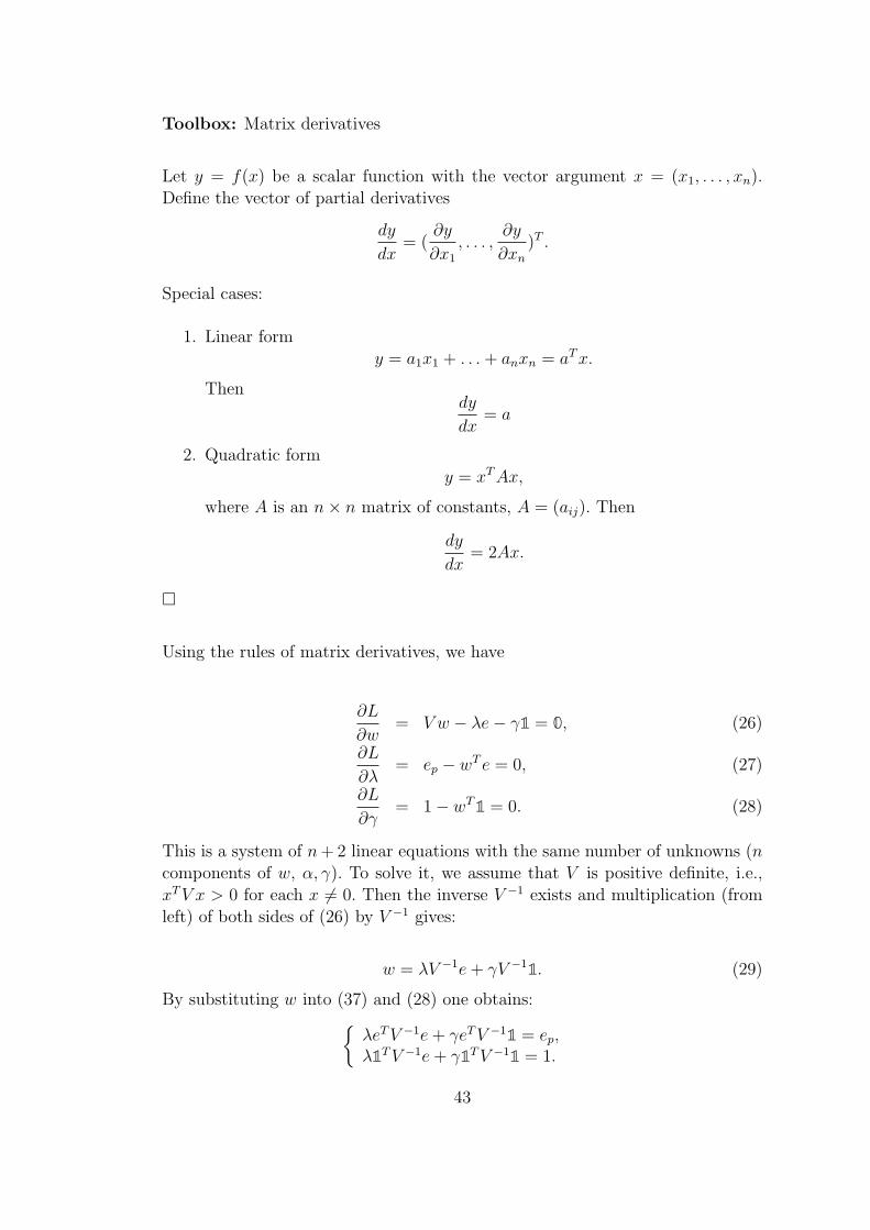
Using the rules of matrix derivatives, we have
∂L
∂w= V w − λe− γ1 = 0, (26)
∂L
∂λ= ep − wT e = 0, (27)
∂L
∂γ= 1− wT1 = 0. (28)
This is a system of n+2 linear equations with the same number of unknowns (ncomponents of w, α, γ). To solve it, we assume that V is positive definite, i.e.,xTV x > 0 for each x = 0. Then the inverse V −1 exists and multiplication (fromleft) of both sides of (26) by V −1 gives:
w = λV −1e+ γV −11. (29)
By substituting w into (37) and (28) one obtains:λeTV −1e+ γeTV −11 = ep,λ1TV −1e+ γ1TV −11 = 1.
43
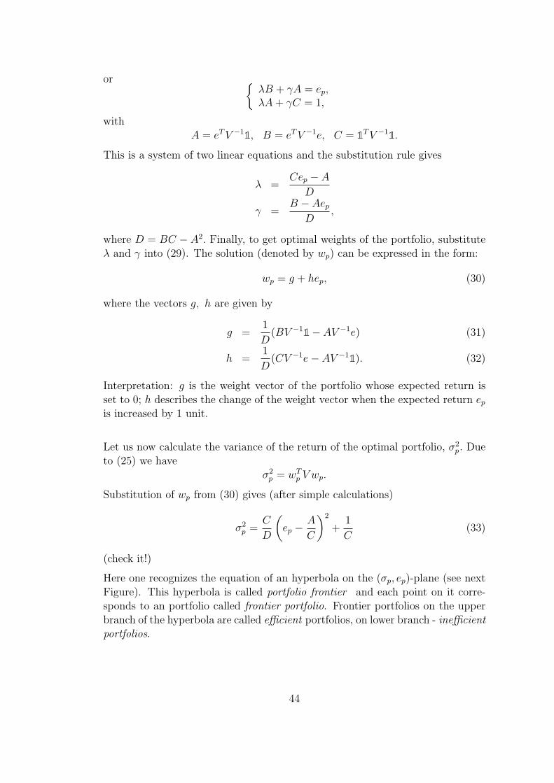
or λB + γA = ep,λA+ γC = 1,
withA = eTV −11, B = eTV −1e, C = 1TV −11.
This is a system of two linear equations and the substitution rule gives
λ =Cep − A
D
γ =B − Aep
D,
where D = BC − A2. Finally, to get optimal weights of the portfolio, substituteλ and γ into (29). The solution (denoted by wp) can be expressed in the form:
wp = g + hep, (30)
where the vectors g, h are given by
g =1
D(BV −11 − AV −1e) (31)
h =1
D(CV −1e− AV −11). (32)
Interpretation: g is the weight vector of the portfolio whose expected return isset to 0; h describes the change of the weight vector when the expected return epis increased by 1 unit.
Let us now calculate the variance of the return of the optimal portfolio, σ2p. Due
to (25) we haveσ2p = wT
p V wp.
Substitution of wp from (30) gives (after simple calculations)
σ2p =
C
D
(ep −
A
C
)2
+1
C(33)
(check it!)
Here one recognizes the equation of an hyperbola on the (σp, ep)-plane (see nextFigure). This hyperbola is called portfolio frontier and each point on it corre-sponds to an portfolio called frontier portfolio. Frontier portfolios on the upperbranch of the hyperbola are called efficient portfolios, on lower branch - inefficientportfolios.
44
6
ep
- σp0
mvp sAC
1C
...........................................................
..........................................................
........................................................
.....................................................
..............................................
.................................................................... ................... ...........
..........................................................................................................................................................................................................................
...........................................................
............................................................
..............................
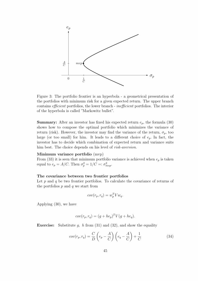
Figure 3: The portfolio frontier is an hyperbola - a geometrical presentation ofthe portfolios with minimum risk for a given expected return. The upper branchcontains efficient portfolios, the lower branch - inefficient portfolios. The interiorof the hyperbola is called ”Markowitz bullet”.
Summary: After an investor has fixed his expected return ep, the formula (30)shows how to compose the optimal portfolio which minimizes the variance ofreturn (risk). However, the investor may find the variance of the return, σp, toolarge (or too small) for him. It leads to a different choice of ep. In fact, theinvestor has to decide which combination of expected return and variance suitshim best. The choice depends on his level of risk-aversion.
Minimum variance portfolio (mvp)From (33) it is seen that minimum portfolio variance is achieved when ep is takenequal to ep = A/C. Then σ2
p = 1/C =: σ2mvp.
The covariance between two frontier portfoliosLet p and q be two frontier portfolios. To calculate the covariance of returns ofthe portfolios p and q we start from
cov(rp, rq) = wTp V wq.
Applying (30), we have
cov(rp, rq) = (g + hep)TV (g + heq).
Exercise: Substitute g, h from (31) and (32), and show the equality
cov(rp, rq) =C
D
(ep −
A
C
)(eq −
A
C
)+
1
C(34)
45

Note that in case of p = q the formula (34) reduces to (33), as required.
46

14 Introducing risk-free assets into the portfolio
The discussion in the previous section, the Markowitz portfolio theory, was basedupon the assumption that the portfolio can only be composed from risky assets(stock, e.g.) In fact, there are always riskless assets available, e.g. short-termgovernment bills, bank account etc. The inclusion of a risk-free asset into themodel is the basic factor that turns the Markowitz theory into so called Capi-tal Asset Pricing Model (CAPM). This innovation is generally regarded as thecontribution of William Sharpe, although Lintner and Mossin developed similartheories at about the same time, in 1960’s.
14.1 Combination of risky portfolio and riskless asset
Interestingly, an investor can improve his or her risk/expected return balance byinvesting partially in a portfolio of risky assets and partially in a risk-free asset.Let us see why this is true.
Consider any portfolio A consisting of n risky assets available on the market ofinterest. The portfolio A can be imagined as a point inside the Markowitz bulletcreated by these assets. Let rA be the return on the portfolio A, eA = E(rA) itsexpected return, and σ2
A the variance of the return (risk on A). Denote by rfthe return on an riskless asset. The term ’riskless’ means that rf is a constant.Compose now a new portfolio c (combined) by investing the fraction X of originalfunds in the portfolio A and the fraction 1−X in the riskless asset. We allow forX to take any non-negative value. A value X > 1 corresponds to the borrowingof additional money (at risk-free rate rf ) and investing it in the portfolio A. Asthe return of the complete portfolio is rc = XrA + (1−X)rf , its expected returnis
ec = XeA + (1−X)rf (35)
and the risk of the combination, since rf is a constant, is
σ2c = D(rc) = D(XrA + (1−X)rf ) = D(XrA) = X2σ2
A.
Henceσc = XσA.
Solving this for X gives
X =σcσA.
Substituting this expression for X into (35) yields
ec =σcσAeA + (1− σc
σA) rf .
47
Rearranging terms,
ec = rf +eA − rfσA
· σc. (36)
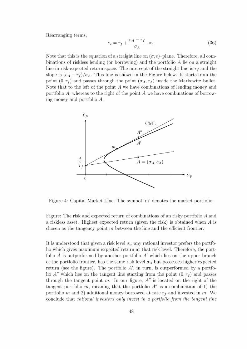
Note that this is the equation of a straight line on (σ, e)–plane. Therefore, all com-binations of riskless lending (or borrowing) and the portfolio A lie on a straightline in risk-expected return space. The intercept of the straight line is rf and theslope is (eA − rf )/σA. This line is shown in the Figure below. It starts from thepoint (0, rf ) and passes through the point (σA, eA) inside the Markowitz bullet.Note that to the left of the point A we have combinations of lending money andportfolio A, whereas to the right of the point A we have combinations of borrow-ing money and portfolio A.
.
....................................................................................................................................................................................................................................................................................................................................................................................................................................................................................................................................................................................................................................................................................................................................................................
......................................................................................................................................................................................................................................................................................................................................................................................................................................................................................................................................................................................................................................................................................
6
ep
- σp0
ACrf
rA = (σA, eA)
rA′
rA′′
sm
CML
...........................................................
..........................................................
........................................................
.....................................................
..............................................
.................................................................... ................... ...........
..........................................................................................................................................................................................................................
...........................................................
............................................................
..............................
Figure 4: Capital Market Line. The symbol ‘m’ denotes the market portfolio.
Figure: The risk and expected return of combinations of an risky portfolio A anda riskless asset. Highest expected return (given the risk) is obtained when A ischosen as the tangency point m between the line and the efficient frontier.
It is understood that given a risk level σc, any rational investor prefers the portfo-lio which gives maximum expected return at that risk level. Therefore, the port-folio A is outperformed by another portfolio A′ which lies on the upper branchof the portfolio frontier, has the same risk level σA but possesses higher expectedreturn (see the figure). The portfolio A′, in turn, is outperformed by a portfo-lio A′′ which lies on the tangent line starting from the point (0, rf ) and passesthrough the tangent point m. In our figure, A′′ is located on the right of thetangent portfolio m, meaning that the portfolio A′′ is a combination of 1) theportfolio m and 2) additional money borrowed at rate rf and invested in m. Weconclude that rational investors only invest in a portfolio from the tangent line
48

and the investors only differ in fractions X and 1 − X they place in m and inriskless asset.
The portfolio m is called market portfolio, and the tangent line is called Cap-ital Market Line (CML). To repeat, the whole CML consists of portfolios thatcan be combined from the portfolio m and risk-free asset by varying their frac-tions X and 1−X (note that X > 1 is allowed, corresponding to the borrowingmoney at rate rf and investing in m).
The term ’market portfolio’ is well justified. Indeed, assuming that all investorsare rational and knowing that a rational investor only invests in m (and partlyin risk-free asset), the weights (w1, . . . , wn) used for investing in n risky assetsare the same for all investors. Therefore the total money invested in the marketfollows the same structure (w1, . . . , wn) i.e. m becomes proportional to marketcapitalizations of n assets.
14.2 Derivation of the Capital Market Line
Our aim here is to derive the weights corresponding to the market portfolio m.By definition, market portfolio maximizes the slope of the straight line (36).Therefore we seek to find weights w = (w1, . . . , wn) of n risky assets in A, subjectto the constraint that
∑ni=1wi = 1, which solves the following maximization
problem:
s :=eA − rfσA
−→ maxw
wT1 = 1.
SinceeA = wT e
andσA = (wTV w)1/2,
the slope s can be expressed as
s =wT e− rf(wTV w)1/2
.
Using Lagrange multipliers, we first define
L =wT e− rf(wTV w)1/2
+ λ(1− wT1).
49
Now take partial derivatives and set the results to zero. Rules of matrix derivationgive
∂L
∂w=
e(wTV w)1/2 − (wTV w)−1/2V w(wT e− rf )
wTV w− λ1 = 0,
∂L
∂λ= wT1 − 1 = 0.
By substituting back wT e = eA and (wTV w)1/2 = σA into the first equation, it iseasy to obtain
σ2Ae− V w(eA − rf ) = σ3
Aλ1. (37)
Multiplication both sides by wT from the left and using wT1 = 1 yields
σ2AeA − σ2
A(eA − rf ) = σ3Aλ.
Henceσ2Arf = σ3
Aλ,
from which we obtainλ =
rfσA.
Substitute this expression for λ into (37) to get
σ2Ae− V w(eA − rf ) = σ2
Arf1.
Rearranging and multiplication of both sides by V −1 gives
eA − rfσ2A
w = V −1(e− rf1). (38)
We can calculate the factoreA−rfσ2A
by multiplying (38) from the left by 1T . As
1Tw = 1, we haveeA − rfσ2A
= 1TV −1(e− rf1) =: δ.
Now, solving (38) for w gives
w =1
δV −1(e− rf1).
As this defines weights of the market portfolio m, we denote the solution by wm:
wm =1
δV −1(e− rf1). (39)
We will use this formula of the market portfolio to derive the CAPM model.
50

We obtain some further insight into (39) by considering a simple case of indepen-dent assets. In such a case V −1 = diag( 1
σ2i) and hence
wi =1
δ· ei − rf
σ2i
,
showing that the higher the expected return of the asset i (normed by its riskσ2i ), the larger is its weight in the portfolio.
As we saw, rational investors only invest in the market portfolio m (and partlyin rf , the weights of m should track the market capitalization. In practise, how-ever, it is not the case. There are several factors why investors are not always’rational’: 1) there are regulators, 2) investors can not afford trading all assetsavailable. Even big investors make choice of 20-40 assets among several hundreds.3) Different investors use different estimates for the model parameters (means,covariances,. ..).
51

15 Capital asset pricing model
The models in the two preceding sections assume that the covariance matrix V isknown. However, financial institutions normally follow n=150 ... 250 securities,and the number of parameters (covariances) to be estimated, n(n+1)/2 is about20 thousand! Hence the models that simplify all analysis are welcome. Capitalasset pricing model was proposed independently by Sharpe, Lintner and Mossinin 1960-s.
More on Market Portfolio
According to our theory all rational investors will invest in the market portfolio,along with some amount of risk-free asset. This has some profound consequencesfor this portfolio. First, the market portfolio must contain all assets on the mar-ket for if an asset is not in the market portfolio, no one will want to purchase itand so the asset will die out.
Since the market portfolio contains all assets, the portfolio has no specific risk-this risk has been diversified out. Thus all risk associated with the market port-folio is systematic risk.
In practice, the market portfolio can be approximated by a much smaller numberof assets. Studies have indicated that a portfolio can achieve a degree of diversi-fication approaching to that of a true market portfolio if it contains a well-choseset of perhaps 20-40 securities. We will use the term market portfolio to refer toan unspecified portfolio that is highly diversified and thus can be considered asessentially free of unsystematic risk.
The risk-return of an asset compared with the market portfolio.
Let us consider any particular asset k in the market portfolio. Our idea is touse the best linear predictor to approximate the return rk on asset k by a linearfunction on the return rm of the entire market portfolio, i.e.
rk = αk + βkrm + ε,
where, as we know from the theory of simple linear regression analysis,
βk =cov(rk, rm)
σ2m
,
αk = ek − βkem,
ek = E(rk)
and ε is the error of the model (residual random variable).
52
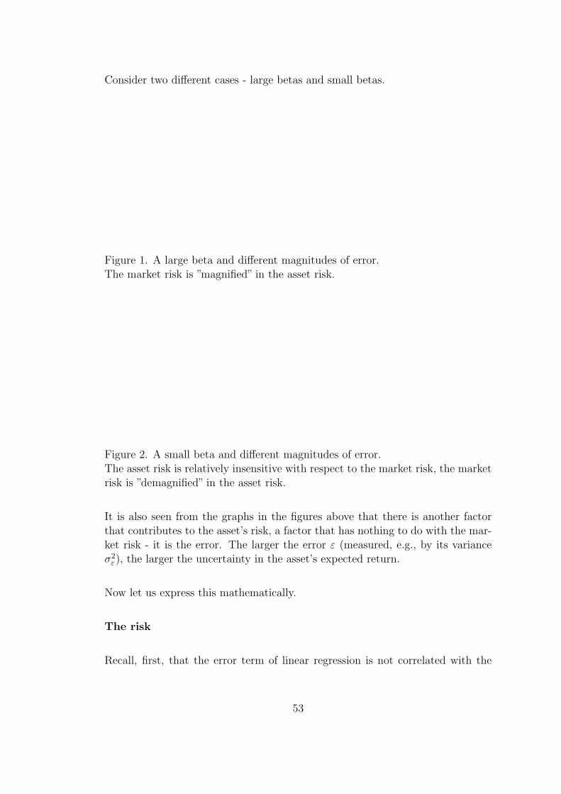
Consider two different cases - large betas and small betas.
Figure 1. A large beta and different magnitudes of error.The market risk is ”magnified” in the asset risk.
Figure 2. A small beta and different magnitudes of error.The asset risk is relatively insensitive with respect to the market risk, the marketrisk is ”demagnified” in the asset risk.
It is also seen from the graphs in the figures above that there is another factorthat contributes to the asset’s risk, a factor that has nothing to do with the mar-ket risk - it is the error. The larger the error ε (measured, e.g., by its varianceσ2ε), the larger the uncertainty in the asset’s expected return.
Now let us express this mathematically.
The risk
Recall, first, that the error term of linear regression is not correlated with the
53

regressor. In our case it means that
cov(rm, ε) = 0.
Therefore the risk associated with the asset k is (since αk is constant)
σ2k = D(rk) = D(αk + βkrm + ε)
= D(βkrm + ε)
= β2kσ
2m + σ2
ε
Thus, the risk of the asset k consists of two components - quantity β2kσ
2m, called
systematic risk, and quantity σ2ε , called unsystematic or unique or idiosyn-
cratic risk. Systematic risk is proportional to the market risk, with a propor-tionality factor of β2
k .
It turns out that, when adding an asset to a diversified portfolio, the unique riskof that asset is canceled out by other assets in the portfolio. Hence, the uniquerisk should not be considered when evaluating the risk-return performance of theasset and so the asset’s beta becomes the crucial point for the risk-return analysisof an asset. Next we will justify this viewpoint.
The expected return
Consider the expected return of the market portfolio
em = eTwm,
where e is the vector of expected returns on all n assets, e = (e1, . . . , en).
The expected return on an individual asset k can be written as
ek = eT1k,
where the vector 1k is defined as
1k = (0, . . . , 0, 1, 0, . . . , 0)T .
To relate these two quantities, we need an expression for e.
Recall that, according to (39), the weights of the market portfolio m verify
wm = δV −1(e− rf1),
where δ is a constant. Solving for e gives
e = δV wm + rf1.
54
We can now write
em = eTwm = (δV wm + rf1)Twm
= δwTmV wm + rf1
Twm
= δσ2m + rf .
In the same way
ek = eT1k = (δV wm + rf1)T1k
= δwTmV 1k + rf1
T1k
= δ · cov(rk, rm) + rf .
Therefore we can express the beta of asset k in terms of expected returns:
βk =cov(rk, rm)
σ2m
=δ(ek − rf )
δ(em − rf )=ek − rfem − rf
.
Finally, solving this for ek gives
ek = βk(em − rf ) + rf .
These important formulae are collected in the following theorem.
Theorem. The expected return and risk of an asset k in the market portfolio isrelated to the asset’s beta as follows:
ek = βk(em − rf ) + rf (40)
and
σ2k = β2
kσ2m + σ2
ε . (41)
The most important observation here is that asset’s expected return dependsonly on the asset’s systematic risk β2
kσ2m (through its beta) and not on its unique
risk σ2ε . This justifies considering only the term β2
kσ2m in assessing the asset’s risk
relative to the market portfolio.
The graph of the line in equation (40) is called security market line (SML).The equation shows that the expected return of an asset is equal to the return ofthe risk-free asset plus the risk premium βk(em − rf ) of the asset. The securitymarket line is shown in the figure below.
Under normal conditions the slope of SML, i.e. em − rf is positive. Hence largebetas imply large expected returns and vice versa. This makes sense - the more(systematic) risk in an asset, the higher should be its expected return under mar-ket equilibrium.
55

The security market line is shown in the following figure.
Figure. The security market line.
Under market equilibrium, all assets should ideally lie on the SML line. Recallthat this assumes rational investors, no investment restrictions, and other con-ditions - the conditions that are never fulfilled entirely. Therefore, in practicethe assets are scattered around the SML, in accordance to their estimated riskand returns. However, the SML has an ’attractive power’ which can be explainedas follows. If an asset is returning less than the market feels is reasonable withrespect to the asset’s perceived risk (the points below the SML), then no onewill buy that asset and its price will decline, thus increasing the asset’s futurereturn. Similarly, if the asset is returning more than the market feel is requiredby the asset’s level of risk (the points above the SML), then more investors willbuy the asset, thus raising its price and lowering its expected return. Thus thereis a tendency for all assets to move closer to SML.
Example.Suppose that the riskfree rate is 3% and that the market portfolio’srisk is 8%. Then the slope of SML is em − rf = 0.08 − 0.03 = 0.05, and thesecurity market equation is
ek = 0.05β + 0.03
We can now compute expected returns under market equilibrium. For example,the value of beta β1 = 1 gives the expected return e1 = 0.08, equal to that ofthe market portfolio. Such an asset has the same systematic risk as the wholemarket (or market portfolio). However, if the beta is less than 1, say β2 = 0.8 ,then the asset has a smaller risk than the market portfolio. Therefore, the marketwill sustain a lower expected return than that of the market portfolio, namelye2 = 0.05× 0.8 + 0.03 = 0.07 < 0.08 = em.
56

16 Value at Risk methodology
Value at risk (VaR) has been called the ”new science of risk management”. Herewe look at the idea behind VAR and the three basic methods of calculating it.
16.1 The idea behind VaR
The most popular and traditional measure of risk is volatility - the standarddeviation of the return of a financial instrument within a specific time horizon.(Standard deviation of the return was used by us as risk measure in three previouschapters devoted to portfolio theory.) The main problem with volatility, however,is that it does not care about the direction of an investment’s movement: a stockcan be volatile because it suddenly jumps higher. However , ifX−EX > 0 then itis good news, and only X−EX < 0 means bad news. Of course, investors are notdistressed by gains! Investors want to measure severity of possible unfavorabledevelopments.
For investors, risk is about the odds of losing money, and VaR is based on thatcommon-sense fact. When calculating VaR, on asks:
• What is the most I can - with a 95% or 99% level of confidence -expect to lose in euros over the next month (year)?
VaR has become the most widely used risk measure in financial institutions, whichhas also made its way into the Basel II capital- adequacy framework. VaR is onepossible approach to risk measurement and it is based on loss distributions. Tolearn about the other approaches (notional amount approach, factor-sensitivitymeasures, scenario-based risk measures), the reader can consult the book byA.McNeil, R.Frey, P.Embrechts Quantitative Risk Management.
16.2 Definition of VaR
According to the idea to measure only unfavorable developments in the value ofassets we introduce the following definition.
Definition 5. The Value at Risk (VaR).
Given the confidence level α ∈ (0, 1], the VaR of the portfolio at the confidencelevel α is given by a smallest number l such that the probability that the loss Lexceeds l is no larger than (1− α). Formally,
V aRα = infl ∈ R : P(L > l) ≤ 1− α = infl ∈ R : FL(l) ≥ α,
where FL is the distribution function of loss.
57
In probabilistic terms, VaR is α-quantile of the loss distribution.
Example
Methods of calculation of VaR:
1. Historical method (see additional .doc file)
2. Parametric approach (e.g. normality assumption)
3. Monte-Carlo method (a ”machinery” needed to generate data)
16.3 Parametric VaR
16.3.1 One financial instrument (one risk factor)
Let us consider a financial instrument e.g. equity (typically, stocks). Let V0, V1, V2, . . . ,be the values of the instrument at time t = 1, 2, . . .. Here the time unit can beday, week, month, quarter, year etc., depending on our time horizon, ∆. Changesin the values of the instrument are most often measured by relative changes, orreturns, defined as
rt =Vt − Vt−1
Vt−1
, t = 1, 2, . . . .
Returns are very often expressed as percentages (in newspapers, TV, other me-dia). Daily returns usually fluctuate within ±1%, and only seldom exceed 3%.Given the return rt, the next value of the asset can be obtained from the previousone by the formula
Vt = Vt−1(1 + rt),
and the change of the asset’s value can be expressed as
Vt − Vt−1 = Vt−1rt. (42)
Naturally, an investor is concerned with possible maximum decrease of the asset’svalue (maximum loss). The formula (42) shows that given the previous value ofthe asset, the loss depends directly on the return rt , and therefore it suffices tofind a critical value r⋆ of the return such that the rt will be smaller than r⋆ onlywith a small probability.
Choice of VaR parameters When working with VaR, we have to choose anappropriate time horizon ∆, and to decide on the confidence level α. There areno single ’right’ values for these parameters, but there are some considerationsthat might influence the choice.
The time horizon ∆ should reflect the time period over which a financial insti-tution is committed to hold its portfolio. For instance, insurance companies aretypically bound to hold their portfolios for one year (mainly 1-year contracts).
58
Hence, ∆ = 1 year is also the appropriate time horizon for measuring the marketrisk of the investment portfolio of such companies.
There are other more practical considerations which suggest that∆ should berelatively small: the use of simplified (linearized) loss formulas is justified if risk-factor changes are small, which is more likely for small ∆. Also, the compositionof the portfolio remains unchanged only with small ∆. Moreover, we have moredata points for estimation of model parameters if ∆ is small.
The confidence level α is given in advance and is often taken as 5%, or 1%, or0,1% etc. However, there are no clear-cut recommendations for the choice of α.For capital adequacy purposes a high confidence level is called for in order tohave sufficient safety margin. For instance, Basel Committee 1 proposes the useof VaR at the 99% level and ∆ equal to 10 days for market risk. In order to setlimits for traders, a bank would typically take 95% and ∆ equal to one day.
16.3.2 Two risk factors
Homework 6. (VaR)
1) An French investor is long (i.e. has a long position of) 200 000 EUR of sharesof a German stock company. The standard deviation of the return of this asset,taken with respect to the time horizon of 10 days, is 1, 22 + 0, 1 · k % (here k isthe last digit of your student ID). Find the critical magnitude l (in EUR) of theloss of the position over a 10 days period, such that the probability that the lossexceeds l is not larger than 0,05 (find VaR).
2) Suppose that the same position is owned by a US investor. It is known thatthe standard deviation of the return of the exchange rate USD/EUR is 0,35%(w.r.t. the same time horizon). The correlation coefficient between the two re-turns equals -0,1.Find the critical magnitude l (in USD) of the loss of the position over a 10 daysperiod, such that the probability that the loss exceeds l is not larger than 0,05(find VaR). Current exchange rate is 0,658 EUR/USD.
Comment the difference between the two answers. What is the cause of the dif-ference?
1The Basel Committee on Banking Supervision (BCBS) is a committee of banking super-visory authorities of 27 countries, whose mandate is to strengthen the regulation, supervisionand practices of banks worldwide.
59

16.4 VaR of the portfolio
(covariances needed)
16.5 Expected shortfall
(as alternative to VaR)
16.6 Coherent risk measures
(with counter-example)
60