risk, return, and ross recovery - faculty web serverfaculty.baruch.cuny.edu/lwu/890/carryu2012.pdf38...
TRANSCRIPT

38 RISK, RETURN, AND ROSS RECOVERY 20TH ANNIVERSARY ISSUE
Risk, Return, and Ross RecoveryPETER CARR AND JIMING YU
PETER CARR
is the executive director of the Masters in Math Finance Program at Courant Institute, New York University in New York, [email protected]
JIMING YU
is a vice president at a large financial institution in New York, NY.
The risk return relation is a staple of modern finance. When risk is measured by volatility, it is well known that option prices convey risk. One of the more inf luential ideas in the last twenty years is that the conditional volatility of an asset price can also be inferred from the market prices of options written on that asset. Under a Markovian restriction, it follows that risk-neutral transition probabilities can also be determined from option prices. Recently, Ross has shown that real-world transition probabilities of a Markovian state vari-able can be recovered from its risk-neutral transition probabilities along with a restriction on preferences. In this article, we show how to recover real-world transition probabilities in a bounded diffusion con-text in a preference-free manner. Our approach is instead based on restricting the form and dynamics of the numeraire portfolio.
Give me a lever long enough and a ful-crum on which to place it, and I shall move the world.
—Archimides
Finance is ultimately the study of the relationship between risk and return. One of the most commonly accepted tenets of this relationship is
that the expected return on an asset increases along with its risk. When risk is measured by volatility, it is widely agreed that option prices convey the degree of risk that the
market forecasts. Yet when it comes to pre-dicting the average return, the conventional wisdom is that option prices are silent in this respect.
Recently, Stephen Ross has written a working paper [2011], that challenges this con-ventional wisdom. Under the assumptions of his model, option prices forecast not only the average return, but also the entire return dis-tribution. Further tweaking the nose of con-ventional wisdom, option prices even convey the conditional return distribution,when the conditioning variable is a Markovian state vari-able that determines aggregate consumption.
Those of us raised on the Black–Merton–Scholes (BMS) paradigm find Ross’s claims to be startling. If one can value options without knowledge of expected return, then how can one use option prices to infer expected return? On the other hand, if expected returns are increasing in volatility, then higher option prices imply higher volatility and higher expected return.
The authors of this article set out to get to the bottom of this conundrum. In trying to understand the foundations of Ross’s model, we discovered an alternative set of sufficient conditions that leads to the same startling conclusion. Our framework is not yet broad enough to encompass the unbounded dif-fusions that describe a standard model such as BMS. Hence, it may well be that option prices are silent regarding expected return
JOD-CARR-CS3.indd 38JOD-CARR-CS3.indd 38 8/23/12 5:34:17 PM8/23/12 5:34:17 PM
The
Jou
rnal
of
Der
ivat
ives
201
2.20
.1:3
8-59
. Dow
nloa
ded
from
ww
w.ii
jour
nals
.com
by
PET
ER
CA
RR
on
09/0
7/12
.It
is il
lega
l to
mak
e un
auth
oriz
ed c
opie
s of
this
art
icle
, for
war
d to
an
unau
thor
ized
use
r or
to p
ost e
lect
roni
cally
with
out P
ublis
her
perm
issi
on.
THE JOURNAL OF DERIVATIVES 3920TH ANNIVERSARY ISSUE
in the BMS model. However, if one is willing to work with bounded diffusions, we discover that option prices can be very vocal about the return distribution of their underlyings.
While Ross’s conclusions do change our world view, there is a hitch. The main restriction on the output of Ross’s model is that the forecast pertains only to a stock market index, which is taken as a proxy for the holdings of the representative agent. If some unimportant asset such as soybeans could not possibly proxy for the entire holdings of the representative agent, then Ross’s model does not provide a forecast. Similarly, if the underlying of an option is regarded as being an asset in zero net supply (e.g., a futures or Chicago Board Options Exchange Volatility Index [VIX2]), then Ross’s model does not provide a forecast. Finally, if the underlying of a cash-settled derivative is not a tradable (e.g., temperature), then forecasts of future values are outside the scope of Ross’s model.
While Ross’s model does not forecast all underly-ings of options, it does provide a forecast of any index such as the S&P 500 Index, which both underlies options and could reasonably be assumed to determine aggregate consumption. This index forecast can be used to reduce prediction error when forecasting financial variables cor-related with such an index. In particular, Ross’s approach can be used to forecast large drops in a broad stock market index and in assets positively correlated with it. As a result, the conclusions of Ross’s model have staggering implica-tions for both financial theory and for the equity index options industry. As the late great economist Paul Samu-elson famously said,“The stock market has forecast nine of the last five recessions.” It will certainly be interesting to see whether the stock index options market can produce a better record than its underlying stock market.
This article has three objectives. The first is to hone in on Theorems 1 and 2 in Ross’s paper and show exactly what has and has not been assumed. The second is to reconcile the standard intuition about the limited role of option prices with Ross’s conclusion that the real-world mean is determined by option prices. The third is to show that one can in fact extend the domain of the forecast to the underlying of any derivative security, even if it is unimportant, not traded, or in zero net supply.
To accomplish the first objective, we provide a review of Ross’s Theorems 1 and 2 in the next section, clarifying both the assumptions and the derivation. In the entire article, we adopt Ross’s notation to ease the task of
comparing results. To accomplish the second objective, we need to pin down the relationship between volatility and expected return. Since there is widespread agreement that option prices forecast volatility, a tight relationship between the spread of returns and the average return would imply the ability to forecast the latter as well.
In the capital asset pricing model (CAPM), the risk–return trade-off is formalized by the observation that in equilibrium, the risk premium on the market portfolio is proportional to its variance and to the risk aversion of the average investor. However, in arbitrage pricing theory, this risk–return trade-off can be formal-ized even more concisely. A little more than 20 years ago, Long [1990] introduced the notion of a numeraire portfolio. As is well known, a numeraire is any self-fi-nancing portfolio whose price is alway positive. Long showed that if any set of assets is arbitrage free, then there always exists a numeraire portfolio comprising just these assets. The defining property of this numeraire portfolio is the following surprising result.1 If the value of the numeraire portfolio is used to def late each asset’s dollar price, then each def lated price evolves as a martingale under the real-world probability measure.
There is an intuition as to why the choice of numeraire changes drift. Suppose the dollar price of an asset is drifting upward as compensation for bearing volatility. If we switch numeraires to the asset itself, then the new price is constant and hence has no drift. More generally, the more positive the correlation between the asset and the numeraire, the closer to zero is the drift. Long showed that one can find a single numeraire that zeros out drift in all relative prices.
Long’s discovery that the numeraire portfolio always exists in arbitrage-free markets allows one to replace the rather abstract probabilistic notion of an equivalent martingale measure with the more concrete and economically grounded notion of the numeraire portfolio. Long also showed that in a multivariate diffusion setting, the risk premium of the numeraire portfolio is its instantaneous variance rate. One could hardly imagine a simpler relationship between expected return and risk. This result is simpler than in the CAPM because no estimate of average risk aversion is required. For the constituents of the numeraire portfolio, the relationship between expected return and risk is only slightly more complex than for the numeraire portfolio itself. In the multivariate diffusion setting, the risk pre-mium of any constituent of the numeraire portfolio is
JOD-CARR-CS3.indd 39JOD-CARR-CS3.indd 39 8/23/12 5:34:17 PM8/23/12 5:34:17 PM
The
Jou
rnal
of
Der
ivat
ives
201
2.20
.1:3
8-59
. Dow
nloa
ded
from
ww
w.ii
jour
nals
.com
by
PET
ER
CA
RR
on
09/0
7/12
.It
is il
lega
l to
mak
e un
auth
oriz
ed c
opie
s of
this
art
icle
, for
war
d to
an
unau
thor
ized
use
r or
to p
ost e
lect
roni
cally
with
out P
ublis
her
perm
issi
on.

40 RISK, RETURN, AND ROSS RECOVERY 20TH ANNIVERSARY ISSUE
the instantaneous covariance of the asset’s return with that of the numeraire portfolio. For further insights on these relations, see Bajeux-Besnainou and Portait [1997]. Note that in a complete market setting such as ours, the covariance of returns between a constituent and the numeraire portfolio is determined by the delta of the constituent w.r.t. the state variable, as we will show.
It follows that if one can determine the implied instantaneous variance of the numeraire portfolio, then one can at least determine its risk premium. If one also knows the risk-free rate, then one knows the expected return of the numeraire portfolio. If one can also determine the covariance of each asset’s return with the numeraire portfolio, then that asset’s expected return can be determined.
Although Ross does not focus on the numeraire portfolio per se, we argue that his assumptions conspire to determine the real-world dynamics of the numeraire portfolio value when one works in a bounded diffusion setting, and when the numeraire portfolio is required to involve all assets. The latter restriction is actually unnec-essary when the goal is to forecast some strict subset of security prices. When Ross’s setting is examined in the bounded diffusion context, the value of the numeraire portfolio is uniquely determined implicitly along with the covariance of each asset’s return on the numeraire portfolio. It follows from the above considerations that each asset’s expected return is also determined in our bounded diffusion setting. Since the returns on each asset depend only on expected return and volatility in a dif-fusion setting, the return distribution for each asset is determined. That Ross is moreover able to determine the real-world return distribution in his jump setting is a tes-tament to the power of his restrictions on preferences.
In our continuous setting, we show that the vola-tility of the numeraire portfolio is the market price of Brownian risk.2 Once this volatility process is determined, the market price of Brownian risk is also determined. Once the market price of Brownian risk is determined in our diffusive setting, we gain clarity on how the real-world dynamics of each asset become determined. The actual mechanics of figuring out the magnitude of instantaneous expected return on each asset is reduced to a straightforward application of Girsanov’s theorem.
To determine the volatility process of the numer-aire portfolio, we must f irst determine its value pro-cess. We follow Ross in assuming that there is a single Markov process X driving all asset prices under con-
sideration. For example, we might restrict ourselves to swaptions of different strikes and maturities and assume that the underlying swap rate drives all of their prices. Markov functional models are in fact commonly used in fixed income (e.g., Hunt, Kennedy, and Pelsser [2000]), although for realism, one usually assumes that two or three Markovian state variables drive some curve or sur-face, rather than the one driving process that Ross uses for simplicity.
Technically, we depart from Ross in assuming that this Markov process is a time-homogeneous reg-ular diffusion, living on a bounded interval of the real line. In contrast, Ross assumes that X is a discrete-time Markov chain with a finite number of states. The uni-variate Markov assumption certainly restricts both of our analyses, but we are optimistic that our work can be extended to higher dimensions. It follows from our univariate diffusion assumption on X that the value of the numeraire portfolio L is also a continuous process under the risk-neutral measure Q. In fact, we will show that the pair (X, L) is a bivariate diffusion. However, we make the stronger assumption that this bivariate diffusion is time homogeneous. We then show that the value function of the numeraire portfolio is uniquely determined from the requirements that it be positive, self-financing, and stationary. This allows us to uniquely determine real-world transition probabilities in our bounded diffusive setting.
Our approach is very similar to the benchmark approach popularized by Platen and co-authors in a series of papers beginning in 2003 (see the references). It turns out that in a wide variety of economic set-tings including ours, the numeraire portfolio also maxi-mizes the real world expected value of the logarithm of terminal wealth. Literature starting with Kelly [1956] and Latané [1959] has described the properties of this so-called “growth optimal” portfolio. Platen and his co-authors advocate using the growth optimal portfolio as a numeraire, due to the martingale property that arises under F. As a result, readers who are familiar with the benchmark approach will likely find our results to be familiar.
Our results provide an alternative set of sufficient conditions that lead to the same qualitative conclusion as in Theorem 1 in Ross [2011]. The common conclu-sion of both articles is that real-world transition prob-abilities are uniquely determined, whether the driver X is a bounded diffusion, as we assume, or a finite-state
JOD-CARR-CS3.indd 40JOD-CARR-CS3.indd 40 8/23/12 5:34:17 PM8/23/12 5:34:17 PM
The
Jou
rnal
of
Der
ivat
ives
201
2.20
.1:3
8-59
. Dow
nloa
ded
from
ww
w.ii
jour
nals
.com
by
PET
ER
CA
RR
on
09/0
7/12
.It
is il
lega
l to
mak
e un
auth
oriz
ed c
opie
s of
this
art
icle
, for
war
d to
an
unau
thor
ized
use
r or
to p
ost e
lect
roni
cally
with
out P
ublis
her
perm
issi
on.
THE JOURNAL OF DERIVATIVES 4120TH ANNIVERSARY ISSUE
Markov chain, as Ross [2011] assumes. Ross’s Theorem 1 assumes complete markets and the existence of a rep-resentative agent whose utility function has a certain structure described below. Ross’s Theorem 1 does not explicitly assume no arbitrage, but Dybvig and Ross [1987, 2003] argue that the absence of arbitrage is equiv-alent to the existence of a representative agent in a par-ticular economic setting. If markets are also complete, then this representative agent is unique. For a description of the economic setting that leads to the existence of a unique representative agent, we quote Ross [2011]:
In a multiperiod model with complete markets and state-independent intertemporally additively separable utility, there is a unique representative agent utility function that satisf ies the above optimum condition and determines the kernel as a function of aggregate consumption (Dybvig and Ross [1987, 2003].
The optimum condition that Ross refers to is Equation (8) below, which will be a major focus of this article. From Ross’s quote above, the economic setting that leads to the existence of a unique representative agent is one with complete markets and multiple indi-viduals whose utility functions are state independent and intertemporally additive separable. Hence, Ross formally derives the conclusion of his Theorem 1 by assuming the existence of a unique representative agent who solves a particular optimization problem described in detail below, but this assumption is itself derived by complete markets and a restriction on preferences of the inhabitants of the economy. If one further assumes that the state variable is a time homogeneous Markov process X with a finite discrete state space, then Theorem 1 in Ross [2011] shows that one can recover the real-world transition probability matrix of X from an assumed known matrix of Arrow–Debreu state prices.
While we have emphasized the staggering implica-tions of this conclusion for equity derivatives, the par-ticular assumptions made in Theorem 1 have several drawbacks. First, Ross is implicitly relying on the Von Neumann–Morgenstern axioms that lead to the con-clusion that all individuals behave as if they maximize expected utility. These axioms have been the subject of much debate. It is difficult to test either the assumptions or the conclusions of the expected utility theorem. The tests that have been done generally conclude that individ-
uals do not behave as if they maximize expected utility, leaving one free to argue that markets behave as if they do. However, empirical tests of stock markets relying on the existence of a representative agent maximizing expected utility (e.g., Hansen and Singleton [1983] and Mehra and Prescott [1985]) have not performed well. We will not attempt to summarize this lengthy debate here, but we refer the interested reader to the Wikipedia entry called “Von Neumann–Morgenstern utility theorem” and the references contained therein. A second draw-back of Ross’s assumptions is the use of an additively separable utility, which rules out both satiation effects and habit formation. One’s utility from consuming sushi for dinner is independent of whether one had sushi at lunch. Likewise, one’s utility from smoking a cigarette is independent of whether one has smoked before. These observations have led to the development of alternative preference specifications (e.g., Kreps and Porteus [1978] and Epstein and Zin [1989]). Indeed, Ross [2011] shows how a recovery theorem in the multinomial context can be developed for Epstein–Zin recursive preferences.
A third drawback of Ross’s assumptions is the use of state-independent utility. While one can aggregate multiple state-independent utility functions into a single state-independent utility function, further restrictions on beliefs or preferences are required in order for this aggregation to occur. When individuals are sufficiently diverse in terms of their probabilities and/or state-in-dependent utilities, it can be impossible to aggregate their preferences into those of a representative agent with state-independent utility (see Mongin [1997]).
While denying the antecedent need not negate the conclusion, there is a more pragmatic reason for seeking a version of Ross’s conclusion that is not based on restricting preferences. The use of the representative agent’s utility function forces the driving process X to be interpreted as a state variable, which by definition includes all random processes that affect aggregate consumption (see Ross’s quote above). This requirement makes it difficult to go from market prices of a particular set of derivatives (e.g., swaptions) to the entire matrix of Arrow–Debreu state prices defined over aggregate consumption.
We accomplish our third objective by replacing Ross’s restrictions on the form of preferences with our restrictions on the form of beliefs (i.e., time-homoge-neous diffusion). To be more specific, let F be the real-world probability measure (as a mnemonic, F denotes frequencies). From the first fundamental theorem of asset
JOD-CARR-CS3.indd 41JOD-CARR-CS3.indd 41 8/23/12 5:34:17 PM8/23/12 5:34:17 PM
The
Jou
rnal
of
Der
ivat
ives
201
2.20
.1:3
8-59
. Dow
nloa
ded
from
ww
w.ii
jour
nals
.com
by
PET
ER
CA
RR
on
09/0
7/12
.It
is il
lega
l to
mak
e un
auth
oriz
ed c
opie
s of
this
art
icle
, for
war
d to
an
unau
thor
ized
use
r or
to p
ost e
lect
roni
cally
with
out P
ublis
her
perm
issi
on.
42 RISK, RETURN, AND ROSS RECOVERY 20TH ANNIVERSARY ISSUE
pricing, no arbitrage implies the existence of a positive F local martingale M, which can be used to create a new probability measure Q equivalent to F via:
d
dM
T T
QddFdd
| =FT
Equivalently, the real-world probability density function (PDF) is given by:
dM
e
Md
T TM
T
t
TT
r dt t
T
F Qdd dd Pdd| =∫
|F FMT TMQ
Md | FT
1 0∫∫
where dT
tr dt tP Qd ed ddt∫−
is the state pricing density.If we know the state pricing density dP, then we
just need to determine the random variable eM
T rtrr dt
T
0∫ in order to determine the real-world PDF dF. We will show that this random variable is just the value of Long’s numeraire portfolio at T. We will impose structure on the real-world dynamics of this numeraire portfolio in order to identify it. In theory, one can identify F either by placing structure on the M and r processes or by placing structure on the numeraire portfolio that Long introduced. Ross takes the former route by linking M to the utility function of the representative agent and by restricting the form of the latter. We take the latter route by placing structure on the dynamics of the numeraire portfolio. We find it easier to assess the reasonableness of a set of restrictions when they are placed on an asset price rather than on one or more utility functions. Besides sample path continuity and a one-dimensional uncertainty, our main restriction on the numeraire portfolio’s returns is that the real-world dynamics are time homogeneous and Markov.
Due to our emphasis on the properties of the numer-aire portfolio, we can take a bottom-up approach to recov-ering F, rather than a top-down approach. We start by identifying an observable (e.g., a swap rate), which enters the payoff of multiple related derivative securities (e.g., swaptions at different strikes). The underlying observable need not determine aggregate consumption, need not be traded, and need not be in positive net supply. We sup-pose that one can also observe prices of a set of derivatives written on this observable underlying. We then suppose that a single Markov process X drives all of these observ-ables. The Markov process X is not required to drive other securities (e.g., stocks). In other words, our Markov pro-cess X need not be a state variable for the entire economy.
Our only requirement on the Markovian driver X is that it affects and determines the valuation of a set of derivative securities whose market prices are known. To the extent that utility functions of investors exist, our only require-ment on them is that more be preferred to less. To the extent that the utility function of the representative agent exists, we allow it to be state dependent, we allow it to not separate across time, and we allow it to be non-stationary. We illustrate our alternative approach by determining the real-world transition probabilities of an interest rate in a single country, when that country has other domestic assets and is part of a multicountry economy.
To summarize, we differ from the Ross paper in two ways. First, on the technical side, we describe the risk-neutral dynamics of the driver by a bounded diffusion rather than a finite state Markov chain. This choice does not affect the qualitative nature of the results: Ross con-clusions also apply in the bounded diffusion setting, and perhaps to some unbounded diffusions as well. Second, and more importantly, we use different sufficient condi-tions to derive the same qualitative conclusion. We place structure on the dynamics of the numeraire portfolio rather than on the preferences of the representative agent. While we grant that this structure can be interpreted as an implicit restriction of preferences, the main point is that the numeraire portfolio need only be composed of assets for which the data are available and the assumptions are appropriate, while the representative agent must always hold all assets in positive net supply. This difference allows us to target our forecast to a wider set of underlyings, while Ross’s forecast is specific to a broad market aggre-gate. We believe that this observation further extends the already substantive impact of Ross’s conclusions con-cerning the informativeness of derivative security prices. Since the forecast applies only out to the longest maturity that one is willing to guess at Arrow–Debreu security prices, one could imagine that the demand for longer-maturity derivatives markets will increase.
An overview of this article is as follows. First, we review the mathematics that Ross uses, in particular, the Perron-Frobenius theorem. We then review Theorems 1 and 2 in Ross. We also review results on regular Sturm—Liouville problems, which we need to convert results on Markov chains to bounded diffusions. Our assumptions are stated in the following section. The subsequent sec-tion shows how we uniquely determine the real-world probability measure from these assumptions. The pen-ultimate section contains an explicit illustration of our
JOD-CARR-CS3.indd 42JOD-CARR-CS3.indd 42 8/23/12 5:34:17 PM8/23/12 5:34:17 PM
The
Jou
rnal
of
Der
ivat
ives
201
2.20
.1:3
8-59
. Dow
nloa
ded
from
ww
w.ii
jour
nals
.com
by
PET
ER
CA
RR
on
09/0
7/12
.It
is il
lega
l to
mak
e un
auth
oriz
ed c
opie
s of
this
art
icle
, for
war
d to
an
unau
thor
ized
use
r or
to p
ost e
lect
roni
cally
with
out P
ublis
her
perm
issi
on.
THE JOURNAL OF DERIVATIVES 4320TH ANNIVERSARY ISSUE
diffusion-based results in a stochastic interest rate setting. We begin the section with a mathematical preliminary concerning spherical harmonics. We end the section by illustrating how the Ross recovery theorem works when the short rate is a simple positive function of a bounded diffusion. The concluding section summarizes the paper and includes suggestions for future research.
MATHEMATICAL PRELIMINARY AND ROSS RECOVERY THEOREM
Mathematical Preliminary: The Perron-Frobenius Theorem
The Perron-Frobenius theorem is a major result in linear algebra that was proved by Oskar Perron and Georg Frobenius. This subsection highlights some of the results and is heavily indebted to the excellent Wikipedia entry “Perron-Frobenius theorem.” Consider the clas-sical eigenvalue problem, where the goal is to find vectors x and scalars λ that solve the system of linear equations:
Ax x= λ
for a given square matrix A. In 1907, Perron proved that if the square matrix A has only strictly positive entries, then there exists a positive real eigenvalue called the principal root, and all other eigenvalues are smaller in absolute value. Corresponding to the principal root is an eigenvector, which has strictly positive components and is unique up to positive scaling. All of the other corre-sponding eigenvectors are not strictly positive (i.e., each one must have entries that are either zero, negative, or complex). In 1912, Frobenius was able to prove similar statements for certain classes of nonnegative matrices called irreducible matrices.
A standard reference to the PF theorem is Meyer [2000], who writes:
In addition to saying something useful, the Per-ron-Frobenius theory is elegant. It is a testament to the fact that beautiful mathematics eventually tends to be useful and useful mathematics eventu-ally tends to be beautiful.
Indeed, the Perron-Frobenius theorem has impor-tant applications to probability theory (ergodicity of Markov chains) and to economics (e.g., Leontief ’s input-output model and Hansen and Scheinkman [2009]’s
long-run economy). In the next subsection, we show how Ross applies the Perron-Frobenius theorem to mathematical finance.
The Ross Recovery Theorem
The goal of the Ross paper is to determine real-world transition probabilities of a Markovian state vari-able X that determines aggregate consumption. Using a snapshot of market prices of derivatives on X, Ross shows how to use time homogeneity of the risk-neutral pro-cess of X, so as to uniquely determine a positive matrix whose elements are Arrow–Debreu security prices. Ross then places sufficient structure on preferences, that is, that there exists a representative agent when utilities are state independent and additively separable, so as to uniquely determine real-world transition probabilities. This last step makes novel use of the Perron-Frobenius theorem covered in the last subsection.
Ross assumes a discrete-time economy, which is described by a finite number n of states of the world. Once one conditions on a state occurring, there is no residual uncertainty. Let F denote the n × n real-world transition matrix, whose entries are the frequencies with which the X process moves from one state to another. As a first cut, Ross requires that from any state, the state variable X must be able to eventually reach any other state. As a result, the matrix F is said to be irreducible and hence amenable to the contribution of Frobenius. Ross also allows the existence of a single absorbing state.
Given that he interprets X as a stock index, this complication is needed to embrace limited liability. However, it is easier to gain intuition on a f irst pass though Ross’s results if we let X be able to exit every state. In fact, it is even easier if the Markovian state vari-able X can transition from any one of the n states in just a single period. In this case, the real-world transition matrix F has only positive entries. In the Ross setup, the magnitude of these positive entries is unknown. All that is known ex ante is that the sum of the n entries in each of the n rows is one. The matrix F is said to be a stochastic matrix, even though the entries are not random variables. In the 2 by 2 case, the output of Ross analysis would be an F matrix such as:
F =. .. .
⎛⎝⎜⎛⎛⎝⎝
⎞⎠⎟⎞⎞⎠⎠
4 6.3 7.
JOD-CARR-CS3.indd 43JOD-CARR-CS3.indd 43 8/23/12 5:34:17 PM8/23/12 5:34:17 PM
The
Jou
rnal
of
Der
ivat
ives
201
2.20
.1:3
8-59
. Dow
nloa
ded
from
ww
w.ii
jour
nals
.com
by
PET
ER
CA
RR
on
09/0
7/12
.It
is il
lega
l to
mak
e un
auth
oriz
ed c
opie
s of
this
art
icle
, for
war
d to
an
unau
thor
ized
use
r or
to p
ost e
lect
roni
cally
with
out P
ublis
her
perm
issi
on.

44 RISK, RETURN, AND ROSS RECOVERY 20TH ANNIVERSARY ISSUE
However, ex ante, all we can say is that:
Ff f
f f=
⎛
⎝
⎜⎛⎛
⎜⎜⎜
⎜⎝⎝
⎜⎜
⎞
⎠
⎟⎞⎞
⎟⎟⎟
⎟⎠⎠
⎟⎟11ff 12ff
21ff 22ff
where f11 > 0, f
12 > 0, f
21 > 0, f
22 > 0, f
11 + f
12 = 1, and
f21
+ f22
= 1.To begin identifying these entries, consider a
second square matrix P whose elements contain prices of single period Arrow-Debreu securities, indexed by both starting state and ending state. In the 2 by 2 case, a typical matrix could look like:
P =. .. .
⎛⎝⎜⎛⎛⎝⎝
⎞⎠⎟⎞⎞⎠⎠
4 5.2 6.
The first row of this matrix indicates that if X starts in state 1, the price of a claim paying $1 if X stays in state 1 is 40 cents, while the price of a claim paying $1 if X instead transitions to state 2 is 50 cents. If X starts in state 1, the price of a zero-coupon bond paying $1 in one period is 90 cents, the sum of the two Arrow–Debreu prices. The second row indicates that if X starts in state 2, the price of this bond is instead 80 cents, the sum of the two Arrow–Debreu state prices indexed by starting state 2.
However, suppose ex ante that we don’t know these AD prices. Then all we can say is that:
Pp p
p p=
⎛
⎝
⎜⎛⎛
⎜⎜⎜
⎜⎝⎝
⎜⎜
⎞
⎠
⎟⎞⎞
⎟⎟⎟
⎟⎠⎠
⎟⎟11 12
21 22
where p11
> 0, p12
> 0, and p22
> 0. Suppose we do not require that interest rates be nonnegative, so we are not requiring that row sums be ≤1. All we require is that the P matrix have strictly positive entries, which is exactly the type of matrix that Perron analyzed. To summarize, P is a positive pricing matrix, while F is a frequency matrix.
Now suppose that we know that X is in state 1 and that we are given a pair of spot prices of single period claims. While this information determines p
11 and p
12,
say p11 = k
11 and p
12 = k
12, the entries p
21 and p
22 remain
undetermined. However, suppose we are also given a pair of spot prices of two-period Arrow–Debreu secu-rites, for examples (b
1, b
2) with both prices in (0, 1).
Suppose we also assume that the risk-neutral process for
X is time homogeneous and that interest rates depend only on X. We then have two linear equations in the two unknowns p
21 and p
22:
k k p b112
12 21 1k p12
and:
k k k p b11 12 12 22 2+ =k p22
Solving for the unknowns gives:
p
b k
k
pb k k
k
211 1k 1
2
12
222 1k 1 1k 2
12
=
= (1)
Unfortunately, these solutions can lie outside [0, 1] if X is not time homogeneous in reality. For example, sup-pose interest rates vanish and that the first-period transi-tion matrix is:
P1PP9 1
9 1=
. .9
. .9
⎛⎝⎜⎛⎛⎝⎝
⎞⎠⎟⎞⎞⎠⎠
Suppose X is actually time inhomogeneous, so that the second-period transition matrix is:
P2PP5 5
5 5=
. .5
. .5
⎛⎝⎜⎛⎛⎝⎝
⎞⎠⎟⎞⎞⎠⎠
Multiplying the two matrices results in:
P P1 2P PP P5 5
5 5=
. .5
. .5
⎛⎝⎜⎛⎛⎝⎝
⎞⎠⎟⎞⎞⎠⎠
An observer in state 1 at time 0 sees just the first row of P
1, (k
11, k
12) = (.9, .1) and the first row of P
1 P
2,
(b1, b
2) = (.5, .5). If the observer assumes that X is time
homogeneous, then the calculation in (1) is:
p21
25
10=
. −5
.<
( )9.
JOD-CARR-CS3.indd 44JOD-CARR-CS3.indd 44 8/23/12 5:34:17 PM8/23/12 5:34:17 PM
The
Jou
rnal
of
Der
ivat
ives
201
2.20
.1:3
8-59
. Dow
nloa
ded
from
ww
w.ii
jour
nals
.com
by
PET
ER
CA
RR
on
09/0
7/12
.It
is il
lega
l to
mak
e un
auth
oriz
ed c
opie
s of
this
art
icle
, for
war
d to
an
unau
thor
ized
use
r or
to p
ost e
lect
roni
cally
with
out P
ublis
her
perm
issi
on.

THE JOURNAL OF DERIVATIVES 4520TH ANNIVERSARY ISSUE
The implied risk-neutral transition probability is negative.
Fortunately, much work has been done on infer-ring a positive risk-neutral transition matrix from option prices. Suppose one starts by assuming that the risk-neu-tral process for the underlying is a time-homogeneous Markov process evolving in continuous time and with a continuous state space. There are two basic approaches for determining these risk-neutral dynamics from a finite set of option prices. The classical approach assumes that the number of parameters describing the underlying is fixed over time. The fixed number of free parameters is typically exceeded by the number of option prices one is trying to fit. Examples include purely continuous processes such as Bachelier [1900], Black and Scholes [1973], Cox [1975], Vasicek [1977], and Cox, Ingersoll, and Ross [1985], pure jump models such as Carr et al. [2002] and Eberlein and Keller [1995], and jump dif-fusions such as Merton [1976] and Kou [2002]. From a finite set of option prices, one does a least-squares fit of the parameters. It is unlikely that the fit is perfect, but the hope is that the error is noise, not a signal that the market is using some other process.
The second approach for determining a time-ho-mogeneous Markov process for the underlying matches the number of parameters with the number of options written on that underlying at the calibration time. These market option prices are assumed to be free of both noise and arbitrage. For example, Carr and Nadtochiy [2012] show how to construct a time-homogeneous Markov process called local variance gamma, which fits a finite number of co-terminal option prices exactly.
Both of the above approaches uniquely determine a time-homogeneous Markov process evolving in con-tinuous time and with a continuous state space. With this risk-neutral process determined, one can then discretize time and space and also truncate the state space. If X is the price of a stock index, then the truncation will be arbitrage free under some mild conditions on carrying cost. If X is the price of a stock index, then arbitrage is avoided at the lowest possible discrete value, if dividend yields are lower than the short rate there. Likewise, if X is the price of a stock index, then arbitrage is avoided at the largest possible discrete value, if dividend yields exceed the short rate there. Fortunately, it is actually realistic to assume that the dividend yield is below the short rate at low prices, while the dividend yield is above the short rate at high prices.
If the dividend on the stock index doesn’t meet these conditions, then avoiding arbitrage makes it necessary to either change the Markov chain to a regular diffusion with inaccessible boundaries, or to change the driver so that it is either the price of some other asset with appro-priate dividends or some function of prices of traded assets (e.g., an interest rate). For example, suppose for simplicity that X is a one-period interest rate, evolving in discrete time as a time-homogeneous two-state Markov chain. If we don’t require that interest rates be positive, then the four unknown elements of the P matrix just need to be positive. There is no martingale condition on a one-period interest rate, so one does not need to restrict car-rying costs as one must do if X is an asset price.
Given these considerations, we are going to just assume that the elements of the pricing matrix P are known and that they are all positive. In the authors’ opinion, the main contribution of the Ross paper is in converting knowledge of a P matrix into knowledge of the F matrix. The main assumptions that allow this identification are complete markets and the existence of a unique representative agent who, in maximizing expected utility f inds it optimal to hold all of the (Arrow–Debreu) securities that trade and engages in exogenous consumption in each period. Quoting from the Ross paper:
The existence of such a representative agent will be a maintained assumption of our analysis below.
We now explore in detail exactly what is presumed by this statement. Just above his Equation (8), Ross for-mally considers an intertemporal model with additively time-separable preferences and a constant discount factor δ > 0. Ross lets the function c(x) denote consumption at time t as a function of the state x that the state variable X
t is in at time t. Letting f(x, y) denote the single-period
real-world transition PDF for the Markov process X, Ross’s Equation (9) reads:
max {aa ( ( )) ( ( )) }
{ ( ) ( )}x( c y(U( x U)) y( f (f ( y d) yd( ( ))U y( f (∫δ
s.t.:
c y p y dy wd( )x )y( ) ( yp+ c( )y (x∫
JOD-CARR-CS3.indd 45JOD-CARR-CS3.indd 45 8/23/12 5:34:18 PM8/23/12 5:34:18 PM
The
Jou
rnal
of
Der
ivat
ives
201
2.20
.1:3
8-59
. Dow
nloa
ded
from
ww
w.ii
jour
nals
.com
by
PET
ER
CA
RR
on
09/0
7/12
.It
is il
lega
l to
mak
e un
auth
oriz
ed c
opie
s of
this
art
icle
, for
war
d to
an
unau
thor
ized
use
r or
to p
ost e
lect
roni
cally
with
out P
ublis
her
perm
issi
on.
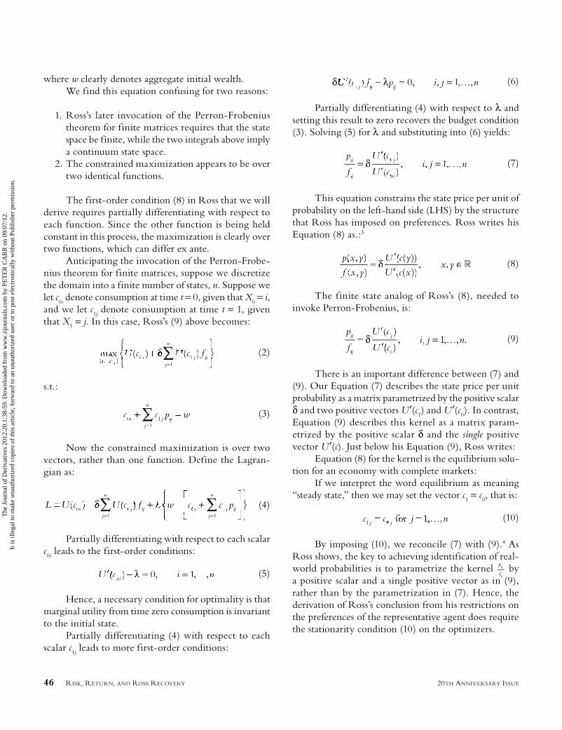
46 RISK, RETURN, AND ROSS RECOVERY 20TH ANNIVERSARY ISSUE
where w clearly denotes aggregate initial wealth.We find this equation confusing for two reasons:
1. Ross’s later invocation of the Perron-Frobenius theorem for finite matrices requires that the state space be finite, while the two integrals above imply a continuum state space.
2. The constrained maximization appears to be over two identical functions.
The first-order condition (8) in Ross that we will derive requires partially differentiating with respect to each function. Since the other function is being held constant in this process, the maximization is clearly over two functions, which can differ ex ante.
Anticipating the invocation of the Perron-Frobe-nius theorem for finite matrices, suppose we discretize the domain into a finite number of states, n. Suppose we let c
0i denote consumption at time t = 0, given that X
0 = i,
and we let c1j denote consumption at time t = 1, given
that X1 = j. In this case, Ross’s (9) above becomes:
x (aa ) ( ){ } i
j
n
j i) jii j
c( c( f ii0 i
01
1=
⎧⎨⎧⎧⎨⎨⎧⎧⎧⎧
⎩⎩⎩⎨⎨⎨⎨
⎫⎬⎫⎫⎬⎬⎫⎫⎫⎫
⎭∑δ ⎬⎬⎬⎬
⎭⎭⎭⎭⎬⎬⎬⎬⎬⎬⎬ (2)
s.t.:
c c wij
n
j ip ji01
1 =c pj p+ 1=
∑∑ (3)
Now the constrained maximization is over two vectors, rather than one function. Define the Lagran-gian as:
L U c pij
n
j jj
n
j ip jiU=j=
∑c i∑ j j∑ −w +( )c ic01
ccj iff j wiff ww1
1δ∑U c f +c ff jiff +⎡⎡
⎣
⎤
⎦⎥⎤⎤
⎦⎦
⎧⎧⎧
⎩⎩⎩
⎫⎬⎪⎫⎫⎬⎬⎭⎪⎬⎬⎭⎭
(4)
Partially differentiating with respect to each scalar c0i leads to the first-order conditions:
′ − = , , ,U ′ …, ni( )c i0 0 1, =i =λ (5)
Hence, a necessary condition for optimality is that marginal utility from time zero consumption is invariant to the initial state.
Partially differentiating (4) with respect to each scalar c
1j leads to more first-order conditions:
δ λ = , = , ,pλλ j, … n,j iff j ipλiff ji( j1 0 1, =i j, (6)
Partially differentiating (4) with respect to λ and setting this result to zero recovers the budget condition (3). Solving (5) for λ and substituting into (6) yields:
p
f
U
Ui j … nij
ijffj
i
=′′
, i = , ,δ( )c j
( )c i
1
0
1 (7)
This equation constrains the state price per unit of probability on the left-hand side (LHS) by the structure that Ross has imposed on preferences. Ross writes his Equation (8) as.:3
p x y
f x y
U y
U xx y
( )x y
)x y
( (c ))
( (c ))= ′
′, x ∈δ R (8)
The finite state analog of Ross’s (8), needed to invoke Perron-Frobenius, is:
p
f
U
Ui j … nij
ijffj
i
=′′
, i = , , .nδ( )c j
( )ci
1 (9)
There is an important difference between (7) and (9). Our Equation (7) describes the state price per unit probability as a matrix parametrized by the positive scalar δ and two positive vectors U ′(c
1) and U ′(c
0). In contrast,
Equation (9) describes this kernel as a matrix param-etrized by the positive scalar δ and the single positive vector U ′(c). Just below his Equation (9), Ross writes:
Equation (8) for the kernel is the equilibrium solu-tion for an economy with complete markets:
If we interpret the word equilibrium as meaning “steady state,” then we may set the vector c
1 = c
0, that is:
c c j … nj j1 0cj c 1jc ,…for (10)
By imposing (10), we reconcile (7) with (9).4 As Ross shows, the key to achieving identification of real-world probabilities is to parametrize the kernel p
fij
ijff by
a positive scalar and a single positive vector as in (9), rather than by the parametrization in (7). Hence, the derivation of Ross’s conclusion from his restrictions on the preferences of the representative agent does require the stationarity condition (10) on the optimizers.
JOD-CARR-CS3.indd 46JOD-CARR-CS3.indd 46 8/23/12 5:34:18 PM8/23/12 5:34:18 PM
The
Jou
rnal
of
Der
ivat
ives
201
2.20
.1:3
8-59
. Dow
nloa
ded
from
ww
w.ii
jour
nals
.com
by
PET
ER
CA
RR
on
09/0
7/12
.It
is il
lega
l to
mak
e un
auth
oriz
ed c
opie
s of
this
art
icle
, for
war
d to
an
unau
thor
ized
use
r or
to p
ost e
lect
roni
cally
with
out P
ublis
her
perm
issi
on.

THE JOURNAL OF DERIVATIVES 4720TH ANNIVERSARY ISSUE
While it is reasonable to believe that the func-tion relating aggregate consumption to state would be stationary, the argument leading to the crucial Equa-tion (9) would be more satisfactory if this stationarity property were derived from prior considerations, rather than imposed as an ad hoc constraint.
Besides stationarity, there is another condition that is being imposed before the validity of Ross’s (8) can be assured. Ross makes explicit that the utility function of the representative agent is state independent. Granting both stationarity and additive separability, we take this to mean that the utility in each period has the form U(c(x)) rather than U(c(x), x). Hence, two states that happen to have the same consumption result in the same utility, regardless of how different the two states are. Kreps and Porteus [1978] show how this leads to indifference toward the timing of the resolution of uncertainty.
We claim that another condition besides state independence is being imposed implicitly. This addi-tional condition is that the optimizing function c(y) is independent of the initial state x of the state variable X determining aggregate consumption. There is nothing in the problem setup that guarantees this kind of state independence. To illustrate, suppose we substitute the stationarity condition (10) into (4):
L ≡ +⎡
⎣
⎤
=∑ ∑− +
⎡⎢⎡⎡
U c∑+ pij
n
j j⎣⎣⎢⎣⎣ j
n
j ip ji( )ci δ∑ ++1 1⎣ =⎣ j ⎦⎦
⎥⎤⎤
⎦⎦⎦⎦
⎧⎧⎧
⎩⎩⎩
⎫⎬⎪⎫⎫⎬⎬⎭⎪⎬⎬⎭⎭
(11)
Now write out the quantities being maximized when n = 2. If the initial state i = 1, then the Lagrangian being maximized is:
L1 1LL 1 11 2 12
1 1 11
≡ ++U c f U11 c f2 1
p1
( )11 [ (U ) (f U11 + ]12f1
{ [
δλ +1 11+c c p1{ [−w − ++ c p2 1p 2 ]} (12)
If the initial state i = 2 instead, then the Lagrangian being maximized is:
L2 2LL 1 21 2 22
2 1 21
≡ ++U c f U21 c f2 2
p1
( )22 [ (U ) (f U21 + ]22f 2
{ [
δλ +2 21+c c p1{ [−w − +++ c p2 2p 2 ]} (13)
Since different Lagrangians are being maximized, the maximizers would depend in general on the initial state. The implicit assumption in Ross’s (8) is that they do not.
Our analysis in the next section is designed to address precisely these issues. Before we proceed with that analysis, we need to show how Ross is able to uniquely determine all of the real-world transition probabilities from the finite-state analog (9) of his key Equation (8). Let:
πiiU
i … n≡′
, =i , ,…1
1( )ic
(14)
be the elements of a positive column vector π. Substi-tuting (14) in (9) implies that:
f
pi j … nijff
ij
j
i
= , =j , ,…1
1δ
ππ
(15)
As we will see, any set of assumptions that lead to the form on the right-hand side (RHS) of (15) also imply uniqueness of the real-world transition probabilities f
ij.
For this reason, we refer to (15) as Ross’s fundamental form. This structure is imposed on the LHS of (15), which is the expected gross return starting from state i of an investment in an Arrow–Debreu security and paying off in state j. In general, this conditional mean return can depend on both the state i that we condition on starting in and on the state j with a positive payoff for an AD security. Hence, if no structure is imposed, one is faced with the gargantuan task of hoping to identify n2 conditional mean returns. If these n2 means could be somehow identified, then each unknown f
ij frequency
could be determined from each corresponding pij price,
since the latter are assumed to be known. Unfortunately, the fact that probabilities sum to one imposes only n linear equations on the n2 unknowns. However, the RHS of (15) indicates that the unknown matrix with entries f
pijff
ij is parametrized by a positive unknown scalar δ and a
positive unknown n × 1 vector π. Hence, the number of unknowns is reduced by the structure on the RHS from n2 to n + 1, and this is before we impose the requirement that probabilities sum to one.
If we now impose these n summing up conditions, it appears that we fall short of our degrees of freedom by a tantalizing single degree. However, it needs to be remembered that all of the n + 1 unknowns on the RHS of (15) are known ex ante to be positive. As Ross shows, this extra set of inequalities are sufficient to uniquely determine the kernel by an appeal to the
JOD-CARR-CS3.indd 47JOD-CARR-CS3.indd 47 8/23/12 5:34:19 PM8/23/12 5:34:19 PM
The
Jou
rnal
of
Der
ivat
ives
201
2.20
.1:3
8-59
. Dow
nloa
ded
from
ww
w.ii
jour
nals
.com
by
PET
ER
CA
RR
on
09/0
7/12
.It
is il
lega
l to
mak
e un
auth
oriz
ed c
opie
s of
this
art
icle
, for
war
d to
an
unau
thor
ized
use
r or
to p
ost e
lect
roni
cally
with
out P
ublis
her
perm
issi
on.

48 RISK, RETURN, AND ROSS RECOVERY 20TH ANNIVERSARY ISSUE
Perron- Frobenius theorem. We now show how Ross pulls the rabbit out of his hat.
Solving (15) for each frequency implies:
f p i j … nijff j
iij ,pij =j , ,…
11
δππ
(16)
Summing over the j index implies:
j
n
ji j
n
j ijipj … n=
∑ ∑ijf ij =p , i , ,…1 1i j=i j
11 1i, i
δπ (17)
since the probabilities sum to one. Re-arranging allows us to write:
j
n
j ij ii iij ii … n=
∑ i = , ,1
1π δj piji (18)
Let P be the n × n matrix with the known elements p
ij > 0, and let π be the n × 1 column vector with the
unknown elements πi > 0. Then (18) can be succinctly
re-expressed as:
Pπ δπ
Here, P is a known positive matrix, while π is an unknown positive vector and δ is an unknown positive scalar.
By the Perron-Frobenius theorem, there exists exactly one positive eigenvector, which is unique up to positive scaling. Corresponding to this eigenvector is the principal eigenvalue, which is positive. We set the rep-resentative agent’s discount factor δ equal to this prin-cipal root. We note that PF theory does not guarantee that the so-called discount factor is below one. If we set the π vector equal to any positive multiple of the prin-cipal eigenvector, then (16) implies that the real-world transition probabilities f
ij become uniquely determined,
since the arbitrary scaling factor divides out. In short, PF theory allows one to uniquely determine F from P, once the structure in (15) is imposed. In the rest of the article, we will focus on a preference-free way to derive this structure.
Before we proceed with that derivation, it needs to be remarked that PF theory has a surprising implica-tion for the determination of F if the single-period bond price pijj
n
=∑ 1 is independent of the state i that X is ini-
tially in. While the assumption that summing out j leads to independence from i seems strained from this per-spective, it needs to be recalled that this independence is equivalent to deterministic interest rates, which is a standard simplifying assumption of well-known equity derivatives pricing models such as Black–Scholes [1973] and Heston [1993].
Whether or not interest rates are deterministic, knowledge of the pricing matrix P implies knowledge of the risk-neutral transition probability matrix Q since:
q p p i j i … nij ijj
n
ij
⎛
⎝⎜⎛⎛
⎝⎝
⎞
⎠⎠⎠, j , ,…
=∑
1
As Ross shows in his Theorem 2, deterministic interest rates imply that the real-world transition prob-ability matrix F obtained via PF theory is equal to this risk-neutral transition probability matrix Q. In other words, the surprising implication is that deterministic interest rates lead to a zero risk premium for all securi-ties.5 Under deterministic interest rates, the P matrix is just the product of the X0−invariant bond price and the stochastic matrix Q. The uniqueness of the principal eigenvalue and the positive eigenvector forces the latter to be a positive multiple of one.
If real-world probabilities must differ from their risk-neutral counterparts, then interest rates must depend on X. When X is forced to be the sole determinant of the representative investor’s consumption, one is forced into building a dependency between interest rates and aggregate consumption that may not exist in reality. This observation makes the development of a theory in which X need not have such a specific role all the more compelling. In the rest of the article, we will focus on a more f lexible theory in which the role of X can be defined according to the derivative security prices that one has on hand.
MATHEMATICAL PRELIMINARY: REGULAR STURM—LIOUVILLE PROBLEM
In this section, we establish a purely mathematical preliminary that allows us to derive Ross’s conclusion from a restriction on beliefs in a diffusion setting. We merely highlight some of the relevant results. This sec-tion is heavily indebted to the excellent Wikipedia entry “Sturm—Liouville Theory.”
JOD-CARR-CS3.indd 48JOD-CARR-CS3.indd 48 8/23/12 5:34:20 PM8/23/12 5:34:20 PM
The
Jou
rnal
of
Der
ivat
ives
201
2.20
.1:3
8-59
. Dow
nloa
ded
from
ww
w.ii
jour
nals
.com
by
PET
ER
CA
RR
on
09/0
7/12
.It
is il
lega
l to
mak
e un
auth
oriz
ed c
opie
s of
this
art
icle
, for
war
d to
an
unau
thor
ized
use
r or
to p
ost e
lect
roni
cally
with
out P
ublis
her
perm
issi
on.

THE JOURNAL OF DERIVATIVES 4920TH ANNIVERSARY ISSUE
We suppose that X is a bounded univariate dif-fusion with drift function b(x) and variance rate a2(x). Using the language of stochastic differential equations (SDEs), X solves the following SDE:
dX b X dt a dWt tb t tdWW+dt= bb , ≥t)t )XXtX ( )Xt 0 (19)
where W is a standard Brownian motion. The process starts at X
0 ∈(�, u), where � and u are both finite. We assume
that a2(x) > 0 on this interval. As a result, the extended generator of X, G I∂
∂∂
∂x x
2 2
22( ) ( ) ( ) , can always be
rewritten in self-adjoint form as G I∂∂
∂∂x∂ x
2
2( )( )x ( ) ( )π
,
where π( ))
( )e)x b y(
a y(dy
≡ ∫�∫22
is a positive function. Consider the Sturm—Liouville problem that arises if we search for functions y(x) and scalars λ that solve:
Gy xG y x( )x ( )x ( )u= − , ∈xλ � (20)
Dividing out the positive function a2
2( )x( )xπ
, this eigen problem has the form:
∂∂
∂∂
− , ∈x x
q y y x w x ∈π λ∂
∂− = −q y( )x )x )x ( )x ( )x ( ),( u,� (21)
where q x V
a( )x ( )x ( )x
( )x≡ 2
2
π is a real-valued function and w
a( )x ( )x
( )x≡ 2
2
π is a positive function. Suppose we further require that π(x), π′(x), q(x), and w(x) be continuous functions over the interval [�,u] and that we have sepa-rated boundary conditions of the form:
α α α1 2 12
220 0α α222y2α( ( )� �α yα2α) (′ = 0α2 (22)
β β β β1 2β 12
220 0β β22y u( )u′ = 0β (23)
Then (21), (22), and (23) are said to be a regular Sturm—Liouville problem.
The main implications of Sturm—Liouville theory for regular Sturm—Liouville problems are:
• The spectrum is discrete and the eigenvalues λ1,
λ2, λ
3, … of the regular Sturm—Liouville problem
(21), (22), and (23) are real and can be ordered such that:
λ λ λ λ1 2λ 3<λ2λ < → ∞λ <n
• Corresponding to each eigenvalue λn is a unique
(up to a normalization constant) eigenfunction y
n(x) which has exactly n−1 zeros in (�,u). The
eigenfunction yn(x) is called the nth fundamental
solution satisfying the regular Sturm—Liouville problem (21), (22), and (23). In particular, the first fundamental solution has no zeros in (�,u) and can always be taken to be positive.
• The normalized eigenfunctions form an ortho-normal basis:
u
n m mnyn y xm w dx∫� =( )x ( )x ( )x δ
in the Hilbert space L2([�,u], w(x)dx). Here, δmn
is a Kronecker delta.
ASSUMPTIONS OF THE MODEL
In this section, we state our assumptions and the implications that each additional assumption has for our analysis. Once all of the assumptions are stated, we derive our main result in the next section.
Our analysis is conducted over a probability space (Ω, F, F) but the probability measure F is not known ex ante. The goal behind the following assumptions is to place restrictions on the measurable space (Ω, F ), on the probability measure F, and on financial markets such that F becomes uniquely identified.
We start by assuming the existence of a money market account:
A1: There exists an asset called a money market account (MMA) whose balance at time t, S
0t, grows at a stochastic
(short) interest rate rt ∈ R:
S et
r dsddt
s
00 0,
∫0 , ≥t (24)
The growth rate r is formally allowed to be real-valued, but in what follows, we will always restrict r to the positive reals. In the language of stochastic differen-tial equations (SDEs), the MMA balance S
0t solves:
r S dt tt0 0t t 0, ,0t t= ,r S dtt0r Str ≥ (25)
subject to the initial condition:
S0 0 1, = (26)
JOD-CARR-CS3.indd 49JOD-CARR-CS3.indd 49 8/23/12 5:34:20 PM8/23/12 5:34:20 PM
The
Jou
rnal
of
Der
ivat
ives
201
2.20
.1:3
8-59
. Dow
nloa
ded
from
ww
w.ii
jour
nals
.com
by
PET
ER
CA
RR
on
09/0
7/12
.It
is il
lega
l to
mak
e un
auth
oriz
ed c
opie
s of
this
art
icle
, for
war
d to
an
unau
thor
ized
use
r or
to p
ost e
lect
roni
cally
with
out P
ublis
her
perm
issi
on.
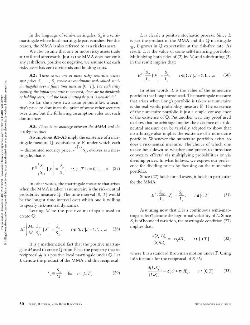
50 RISK, RETURN, AND ROSS RECOVERY 20TH ANNIVERSARY ISSUE
In the language of semi-martingales, S0 is a semi-
martingale whose local martingale part vanishes. For this reason, the MMA is also referred to as a riskless asset.
We also assume that one or more risky assets trade at t = 0 and afterwards. Just as the MMA does not emit any cash f lows, positive or negative, we assume that each risky asset has zero dividends and holding costs.
A2: There exists one or more risky securities whose spot prices S
1, …, S
n evolve as continuous real-valued semi-
martingales over a finite time interval [0, T ]. For each risky security, the initial spot price is observed, there are no dividends or holding costs, and the local martingale part is non-trivial.
So far, the above two assumptions allow a secu-rity’s price to dominate the price of some other security over time, but the following assumption rules out such dominance:
A3: There is no arbitrage between the MMA and the n risky securities.
Assumptions A1-A3 imply the existence of a mar-tingale measure Q, equivalent to F, under which each
r− discounted security price, e St
sr dsdd
it
− ∫ , evolves as a mar-tingale, that is.
ES
S
S
StiT
Tt
it
t
Q
0 0ST
| =t , ∈t⎧
⎨⎪⎧⎧⎪⎨⎨⎪⎪
⎩⎪⎨⎨
⎪⎩⎩⎪⎪
⎫⎪⎫⎫⎪⎪
⎭⎪⎪⎭⎭⎪⎪Ft [ ] 0T i0, ,T = 100, ,1 ,… n, (27)
In other words, the martingale measure that arises when the MMA is taken as numeraire is the risk-neutral probability measure Q. The time interval [0, T ] would be the longest time interval over which one is willing to specify risk-neutral dynamics.
Letting M be the positive martingale used to create Q:
EM
M
S
S
S
StT
t
iT
Tt
it
t
F
0 0ST
| =t , ∈t⎧
⎨⎪⎧⎧⎪⎨⎨⎪⎪
⎩⎪⎨⎨
⎪⎩⎩⎪⎪
⎫⎪⎫⎫⎪⎪
⎭⎪⎪⎭⎭⎪⎪Ft [ ]T0, ]], = , , ,i …= , n0 1,, (28)
It is a mathematical fact that the positive martin-gale M used to create Q from F has the property that its reciprocal 1
M is a positive local martingale under Q. Let
L denote the product of the MMA and this reciprocal:
LS
Mtt
t
t
≡ ,M
t0 for [ ]T, (29)
L is clearly a positive stochastic process. Since L is just the product of the MMA and the Q martingale 1M
, L grows in Q expectation at the risk-free rate. As result, L is the value of some self-financing portfolio. Multiplying both sides of (2) by M
t and substituting (3)
in the result implies that:
ES
L
S
LtiT
Tt
it
t
F | =t , ∈t , = ,⎧
⎨⎪⎧⎧
⎨⎨⎪⎪⎨⎨⎨⎨
⎩⎪⎨⎨
⎩⎩⎪⎪⎩⎩⎩⎩
⎫⎪⎫⎫⎪⎪
⎭⎪⎭⎭⎪⎪⎭⎭⎭⎭
Ft [ ]T, 0i, =]T,T 11, ,… n, (30)
In other words, L is the value of the numeraire portfolio that Long introduced. The martingale measure that arises when Long’s portfolio is taken as numeraire is the real-world probability measure F. The existence of the numeraire portfolio is just a simple consequence of the existence of Q. Put another way, any proof used to show that no arbitrage implies the existence of a risk-neutral measure can be trivially adapted to show that no arbitrage also implies the existence of a numeraire portfolio. Whenever the numeraire portfolio exists, so does a risk-neutral measure. The choice of which one to use boils down to whether one prefers to introduce convexity effects6 via multiplying probabilities or via dividing prices. In what follows, we express our prefer-ence for dividing prices by focusing on the numeraire portfolio.
Since (27) holds for all assets, it holds in particular for the MMA:
ES
L
S
LtT
Tt
t
t
F 0 0ST | =t , ∈t⎧
⎨⎪⎧⎧
⎨⎨⎪⎪⎨⎨⎨⎨
⎩⎪⎨⎨
⎩⎩⎪⎪⎩⎩⎩⎩
⎫⎪⎫⎫⎪⎪
⎭⎪⎭⎭⎪⎪⎭⎭⎭⎭
t [ ]T0, (31)
Assuming now that L is a continuous semi-mar-tingale, let σ
t denote the lognormal volatility of L. Since
S0 is of bounded variation, the martingale condition (27)
implies that:
d S
dB tt
tt tdB
( )S L
( )S L[ ]T0
0
LL
LL= − , ∈tσ (32)
where B is a standard Brownian motion under F. Using Itô’s formula for the reciprocal of S
0/L:
d L
d dB tt
tt t t
( )L S
( )L S[ ]T
S= +dt , ∈t0
0
2σ σt dt +dtt dt (33)
JOD-CARR-CS3.indd 50JOD-CARR-CS3.indd 50 8/23/12 5:34:21 PM8/23/12 5:34:21 PM
The
Jou
rnal
of
Der
ivat
ives
201
2.20
.1:3
8-59
. Dow
nloa
ded
from
ww
w.ii
jour
nals
.com
by
PET
ER
CA
RR
on
09/0
7/12
.It
is il
lega
l to
mak
e un
auth
oriz
ed c
opie
s of
this
art
icle
, for
war
d to
an
unau
thor
ized
use
r or
to p
ost e
lect
roni
cally
with
out P
ublis
her
perm
issi
on.
THE JOURNAL OF DERIVATIVES 5120TH ANNIVERSARY ISSUE
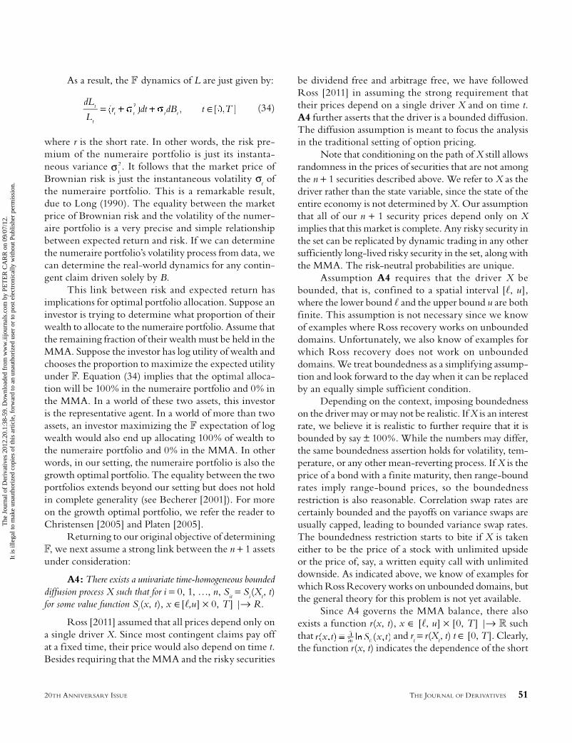
As a result, the F dynamics of L are just given by:
dL
Ldt dB tt
tt t t t= + ,dBt tdB ∈( )r(rt trrr [ ]T,dt)t
2 (34)
where r is the short rate. In other words, the risk pre-mium of the numeraire portfolio is just its instanta-neous variance σt
2. It follows that the market price of Brownian risk is just the instantaneous volatility σ
t of
the numeraire portfolio. This is a remarkable result, due to Long (1990). The equality between the market price of Brownian risk and the volatility of the numer-aire portfolio is a very precise and simple relationship between expected return and risk. If we can determine the numeraire portfolio’s volatility process from data, we can determine the real-world dynamics for any contin-gent claim driven solely by B.
This link between risk and expected return has implications for optimal portfolio allocation. Suppose an investor is trying to determine what proportion of their wealth to allocate to the numeraire portfolio. Assume that the remaining fraction of their wealth must be held in the MMA. Suppose the investor has log utility of wealth and chooses the proportion to maximize the expected utility under F. Equation (34) implies that the optimal alloca-tion will be 100% in the numeraire portfolio and 0% in the MMA. In a world of these two assets, this investor is the representative agent. In a world of more than two assets, an investor maximizing the F expectation of log wealth would also end up allocating 100% of wealth to the numeraire portfolio and 0% in the MMA. In other words, in our setting, the numeraire portfolio is also the growth optimal portfolio. The equality between the two portfolios extends beyond our setting but does not hold in complete generality (see Becherer [2001]). For more on the growth optimal portfolio, we refer the reader to Christensen [2005] and Platen [2005].
Returning to our original objective of determining F, we next assume a strong link between the n + 1 assets under consideration:
A4: There exists a univariate time-homogeneous bounded diffusion process X such that for i = 0, 1, …, n, S
it = S
i(X
t, t)
for some value function Si(x, t), x ∈[�,u] × 0, T ] |→ R.
Ross [2011] assumed that all prices depend only on a single driver X. Since most contingent claims pay off at a fixed time, their price would also depend on time t. Besides requiring that the MMA and the risky securities
be dividend free and arbitrage free, we have followed Ross [2011] in assuming the strong requirement that their prices depend on a single driver X and on time t. A4 further asserts that the driver is a bounded diffusion. The diffusion assumption is meant to focus the analysis in the traditional setting of option pricing.
Note that conditioning on the path of X still allows randomness in the prices of securities that are not among the n + 1 securities described above. We refer to X as the driver rather than the state variable, since the state of the entire economy is not determined by X. Our assumption that all of our n + 1 security prices depend only on X implies that this market is complete. Any risky security in the set can be replicated by dynamic trading in any other sufficiently long-lived risky security in the set, along with the MMA. The risk-neutral probabilities are unique.
Assumption A4 requires that the driver X be bounded, that is, confined to a spatial interval [�, u], where the lower bound � and the upper bound u are both finite. This assumption is not necessary since we know of examples where Ross recovery works on unbounded domains. Unfortunately, we also know of examples for which Ross recovery does not work on unbounded domains. We treat boundedness as a simplifying assump-tion and look forward to the day when it can be replaced by an equally simple sufficient condition.
Depending on the context, imposing boundedness on the driver may or may not be realistic. If X is an interest rate, we believe it is realistic to further require that it is bounded by say ± 100%. While the numbers may differ, the same boundedness assertion holds for volatility, tem-perature, or any other mean-reverting process. If X is the price of a bond with a finite maturity, then range-bound rates imply range-bound prices, so the boundedness restriction is also reasonable. Correlation swap rates are certainly bounded and the payoffs on variance swaps are usually capped, leading to bounded variance swap rates. The boundedness restriction starts to bite if X is taken either to be the price of a stock with unlimited upside or the price of, say, a written equity call with unlimited downside. As indicated above, we know of examples for which Ross Recovery works on unbounded domains, but the general theory for this problem is not yet available.
Since A4 governs the MMA balance, there also exists a function r(x, t), x ∈ [�, u] × [0, T ] |→ R such that r St( )x t l ( )x t)t ∂
∂ 0 and r
t = r(X
t, t) t ∈ [0, T]. Clearly,
the function r(x, t) indicates the dependence of the short
JOD-CARR-CS3.indd 51JOD-CARR-CS3.indd 51 8/23/12 5:34:21 PM8/23/12 5:34:21 PM
The
Jou
rnal
of
Der
ivat
ives
201
2.20
.1:3
8-59
. Dow
nloa
ded
from
ww
w.ii
jour
nals
.com
by
PET
ER
CA
RR
on
09/0
7/12
.It
is il
lega
l to
mak
e un
auth
oriz
ed c
opie
s of
this
art
icle
, for
war
d to
an
unau
thor
ized
use
r or
to p
ost e
lect
roni
cally
with
out P
ublis
her
perm
issi
on.
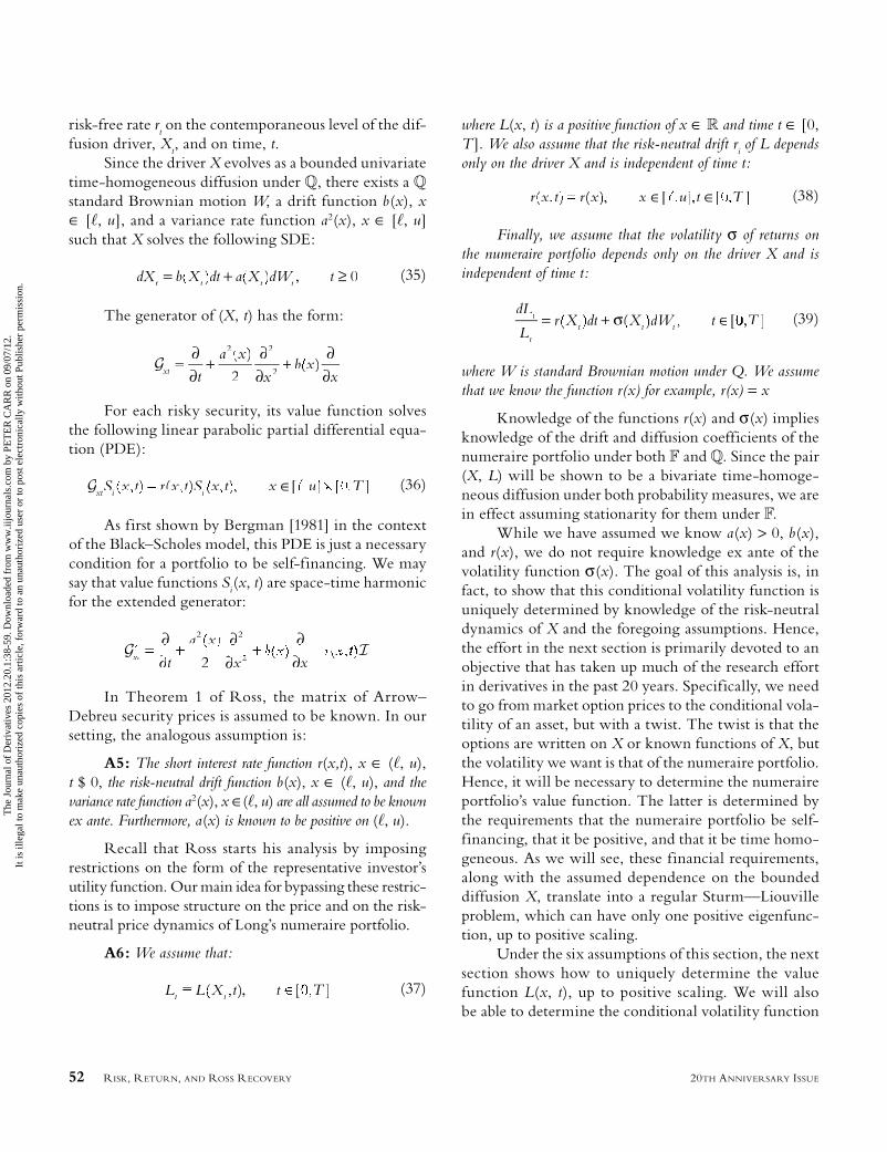
52 RISK, RETURN, AND ROSS RECOVERY 20TH ANNIVERSARY ISSUE
risk-free rate rt on the contemporaneous level of the dif-
fusion driver, Xt, and on time, t.
Since the driver X evolves as a bounded univariate time-homogeneous diffusion under Q, there exists a Q standard Brownian motion W, a drift function b(x), x ∈ [�, u], and a variance rate function a2(x), x ∈ [�, u] such that X solves the following SDE:
dX b X dt a dWt tb t tdWW+dt= bb , ≥t)tX )XXtX ( )Xt 0 (35)
The generator of (X, t) has the form:
GxtGG t
a
xb x
x=
∂∂
+∂
∂+
∂∂
2 2∂22
( )x( )x
For each risky security, its value function solves the following linear parabolic partial differential equa-tion (PDE):
GxtGG i iSi r S x( )x t ( )x t ( )x t [ ] [ ]Tt iSi)t (x , ∈x ]u� (36)
As first shown by Bergman [1981] in the context of the Black–Scholes model, this PDE is just a necessary condition for a portfolio to be self-financing. We may say that value functions S
i(x, t) are space-time harmonic
for the extended generator:
G IxtGG t
a
x x
∂∂
∂∂
∂∂
2 2∂22
( )x( ) ( ),
In Theorem 1 of Ross, the matrix of Arrow– Debreu security prices is assumed to be known. In our setting, the analogous assumption is:
A5: The short interest rate function r(x,t), x ∈ (�, u), t $ 0, the risk-neutral drift function b(x), x ∈ (�, u), and the variance rate function a2(x), x ∈(�, u) are all assumed to be known ex ante. Furthermore, a(x) is known to be positive on (�, u).
Recall that Ross starts his analysis by imposing restrictions on the form of the representative investor’s utility function. Our main idea for bypassing these restric-tions is to impose structure on the price and on the risk-neutral price dynamics of Long’s numeraire portfolio.
A6: We assume that:
L L tt tLL , ∈t( )X tt ,XtX [ ]T, (37)
where L(x, t) is a positive function of x ∈ R and time t ∈ [0, T ]. We also assume that the risk-neutral drift r
i of L depends
only on the driver X and is independent of time t:
r r t( )x t ( )x [ ]u [ ]T)t , ∈x ,]u ∈[� (38)
Finally, we assume that the volatility σ of returns on the numeraire portfolio depends only on the driver X and is independent of time t:
dL
Lr d X dW tt
tt tdt tWW= +r dtdt , ∈t( )XtXt ( )XtX [ ]T,σ (39)
where W is standard Brownian motion under Q. We assume that we know the function r(x) for example, r(x) = x
Knowledge of the functions r(x) and σ(x) implies knowledge of the drift and diffusion coefficients of the numeraire portfolio under both F and Q. Since the pair (X, L) will be shown to be a bivariate time-homoge-neous diffusion under both probability measures, we are in effect assuming stationarity for them under F.
While we have assumed we know a(x) > 0, b(x), and r(x), we do not require knowledge ex ante of the volatility function σ(x). The goal of this analysis is, in fact, to show that this conditional volatility function is uniquely determined by knowledge of the risk-neutral dynamics of X and the foregoing assumptions. Hence, the effort in the next section is primarily devoted to an objective that has taken up much of the research effort in derivatives in the past 20 years. Specifically, we need to go from market option prices to the conditional vola-tility of an asset, but with a twist. The twist is that the options are written on X or known functions of X, but the volatility we want is that of the numeraire portfolio. Hence, it will be necessary to determine the numeraire portfolio’s value function. The latter is determined by the requirements that the numeraire portfolio be self-financing, that it be positive, and that it be time homo-geneous. As we will see, these financial requirements, along with the assumed dependence on the bounded diffusion X, translate into a regular Sturm—Liouville problem, which can have only one positive eigenfunc-tion, up to positive scaling.
Under the six assumptions of this section, the next section shows how to uniquely determine the value function L(x, t), up to positive scaling. We will also be able to determine the conditional volatility function
JOD-CARR-CS3.indd 52JOD-CARR-CS3.indd 52 8/23/12 5:34:22 PM8/23/12 5:34:22 PM
The
Jou
rnal
of
Der
ivat
ives
201
2.20
.1:3
8-59
. Dow
nloa
ded
from
ww
w.ii
jour
nals
.com
by
PET
ER
CA
RR
on
09/0
7/12
.It
is il
lega
l to
mak
e un
auth
oriz
ed c
opie
s of
this
art
icle
, for
war
d to
an
unau
thor
ized
use
r or
to p
ost e
lect
roni
cally
with
out P
ublis
her
perm
issi
on.
THE JOURNAL OF DERIVATIVES 5320TH ANNIVERSARY ISSUE
σ(x) uniquely. This implies that we uniquely determine both the market price of Brownian risk, which is σ(x), and the risk premium of the numeraire portfolio which is σ2(x). Finally, we uniquely determine the dynamics of X under F and the real-world probability measure F itself.
ANALYSIS
Imposing A6 on (34) implies that the F dynamics of L are given by:
dL
LX X dt dB tt
tt t t t= Xt + ,dBtdB ≥[ (rr ) + ( )] ( )XtXtdtXtX( )]2 0
where recall that B is a standard Brownian motion under F. Applying Itô’s formula to (37), the volatility of L is:
σ( )( )
( ) ( ) ( ) ln ( )L( x)
L( a) a)x
L(≡∂
∂=) ( )a) )
∂∂
1 (40)
From A5, a(x) is known to be positive on (�, u). Dividing by a(x) and integrating w.r.t. x:
ln ( , )( )
( ))L( t
a y(dy f t(
x= +
( )ydy∫
σ
where f(t) is the constant of integration. Exponentiating implies that the value of the numeraire portfolio sepa-rates multiplicatively into a positive function π(⋅) of the driver X and a positive function p(⋅) of time t:
L p t( )x t ( )x ( )t)t π (41)
where
πσ
( )( )( )e)
x ya y(
dy∫
and
p t e f t( )t )t=
Substituting (38) and (41) into the PDE (36) implies:
π π π( ) ( )( )
( ) ( ) ( ) ( ) ( ) (p)a (
x p) t b) π) ( p t( r′ + ′′ ′ =2
2x xxx p x) ( ) (p )
Dividing by π(x) p(t) implies:
ab x r
p t
p
2
2
( )x ( )x
( )x( )x
( )x
( )x( )x( )x
( )t′′ + ′ − =r )x − ′ππ
ππ ( )((
( ) [ ]x t [
,
∈(( , ∈t�
The two sides can only be equal if they are each equal to a constant, say −λ ∈ R. In that case, we have two ordinary differential equations (ODE’s):
′ = ,p t′p t
t ∈( );t( );t
[ ],T,λλ
λ (42)
and:
ab r x
2
2
( )x( ) ( )x ( ) ( )x ( ) () −) =)π λ(x′′ π λ(x′ π λ(x λπ ; ,;;
∈
λ)
( ),,x ∈ � (43)
The general solution to (42) is:
p t p e t( )t ))λ λp) (=) λ (44)
Without loss of generality, we may set p(0) = 1 so that:
p t e t( )t =)λ λ (45)
Substituting (45) in (41) implies that the form for the value function of the numeraire portfolio must be:
L e t( )x t ( )x ( )u)t , ∈xπ λ � (46)
where π (x) is a positive function solving the ODE (43).
This ODE can be regarded as a regular Sturm—Liouville problem.7 One can numerically solve for all of the eigenfunctions and eigenvalues. From the sec-tion before last, we know that the smallest eigenvalue is unique, and we will call it ρ. When the eigenvalues are ordered from smallest to largest, ρ is the first eigenvalue. Associated to ρ is an eigenfunction, which is unique up to positive scaling. We will call this f irst eigenfunc-tion φ(x), understanding that the positive scale factor is indeterminate. This first eigenfunction is positive, that is, φ(x) > 0. All of the eigenfunctions associated to the
JOD-CARR-CS3.indd 53JOD-CARR-CS3.indd 53 8/23/12 5:34:22 PM8/23/12 5:34:22 PM
The
Jou
rnal
of
Der
ivat
ives
201
2.20
.1:3
8-59
. Dow
nloa
ded
from
ww
w.ii
jour
nals
.com
by
PET
ER
CA
RR
on
09/0
7/12
.It
is il
lega
l to
mak
e un
auth
oriz
ed c
opie
s of
this
art
icle
, for
war
d to
an
unau
thor
ized
use
r or
to p
ost e
lect
roni
cally
with
out P
ublis
her
perm
issi
on.
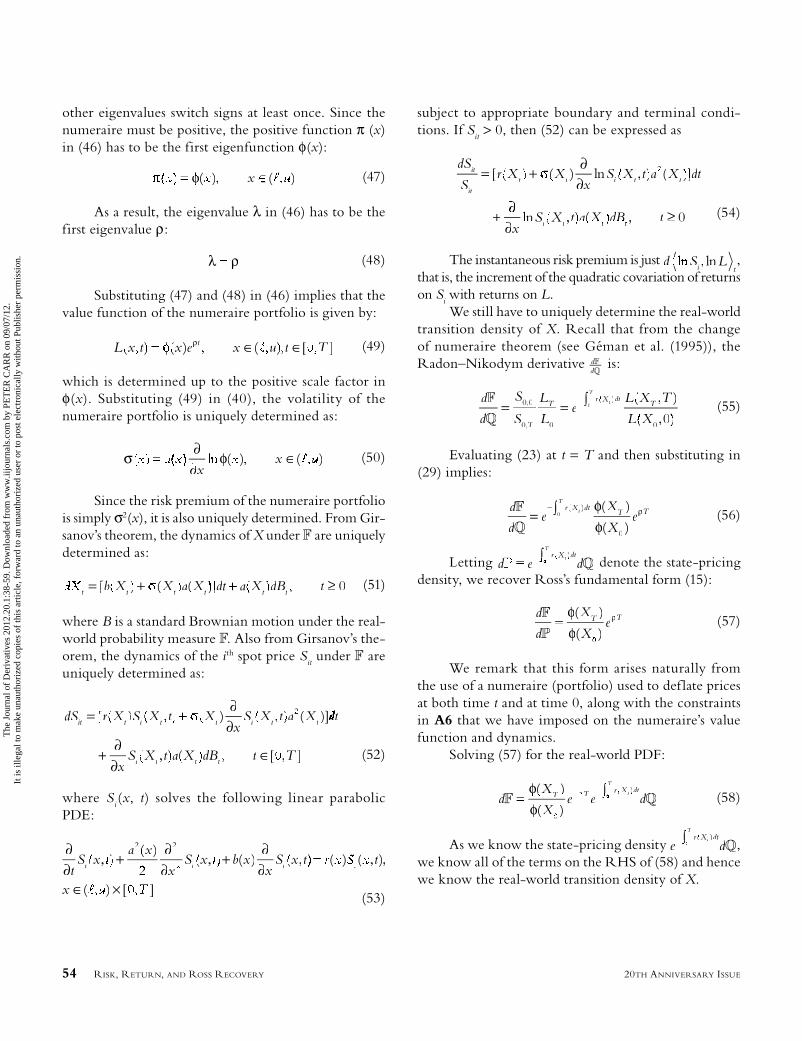
54 RISK, RETURN, AND ROSS RECOVERY 20TH ANNIVERSARY ISSUE
other eigenvalues switch signs at least once. Since the numeraire must be positive, the positive function π (x) in (46) has to be the first eigenfunction φ(x):
( ) ( )φ( x,φ( )φ( ∈((� (47)
As a result, the eigenvalue λ in (46) has to be the first eigenvalue ρ:
λ ρ (48)
Substituting (47) and (48) in (46) implies that the value function of the numeraire portfolio is given by:
L e tt( )x t ( )x ( )u [ ]T)t , ∈x ,)u ∈[φ ρ � (49)
which is determined up to the positive scale factor in φ(x). Substituting (49) in (40), the volatility of the numeraire portfolio is uniquely determined as:
σ φl ( ) ( )x
)∂
∂, ∈x � (50)
Since the risk premium of the numeraire portfolio is simply σ2(x), it is also uniquely determined. From Gir-sanov’s theorem, the dynamics of X under F are uniquely determined as:
b X X X dt X dB tt tX t tX t tX= tX + ,a dBtdB ≥[bbbb ) (+ ) (aa )] (XtXt 0 (51)
where B is a standard Brownian motion under the real-world probability measure F. Also from Girsanov’s the-orem, the dynamics of the ith spot price S
it under F are
uniquely determined as:
dS X X t Xx
X t Xit t i t tt X i tX t= ,X Xt t
∂∂
,[ (rr ) (SiSiS ) ( ) (Si
∂∂
) (a )]2 dtdd
xS a X dB ti t t t+
∂∂
,dBtdBa ∈( )X ttX ,t ( t(XXt [ ]T, (52)
where Si(x, t) solves the following linear parabolic
PDE:
∂∂
+∂
∂∂
∂,
tS
a
xS t b+
xS x ti i+
∂S i( ),x,x
( )x( ),x ( )x (
2 2∂( )22
) ()) ) ( )
( ) [ ]
,( ) ( ,
(∈( × [
x(( x(( t
x ∈(
i
� (53)
subject to appropriate boundary and terminal condi-tions. If S
it > 0, then (52) can be expressed as
dS
SX X
xX t X dtit
itt tX i tX tXt=
∂∂
,
+
[ (r[ (r ) (+ ) l∂
∂n (Si ) (a )]2
∂∂∂
, ≥x
S a X dB t,i t t tln ( ),X ttX (Xt 0 (54)
The instantaneous risk premium is just d S Li tln, ,
that is, the increment of the quadratic covariation of returns on S
i with returns on L.We still have to uniquely determine the real-world
transition density of X. Recall that from the change of numeraire theorem (see Géman et al. (1995)), the Radon–Nikodym derivative d
dFddQdd is:
d
d
S
S
L
Le
L
L XT
T r dt T
T
tFddQdd
= = ∫,
,
,
−0 0,
0 0LT, 0
0∫∫0
( )Xt ( )X TT ,( ))
(55)
Evaluating (23) at t = T and then substituting in (29) implies:
d
de e
T
tr dt T TFddQdd
= ∫−0∫∫
0
( )tX ( )XT
( )X 0
φφ
ρ (56)
Letting dT
r dtP Qd ed ddt∫− ( )tXt denote the state-pricing
density, we recover Ross’s fundamental form (15):
d
deT TFdd
Pdd=
φφ
ρ( )XT
( )X 0
(57)
We remark that this form arises naturally from the use of a numeraire (portfolio) used to def late prices at both time t and at time 0, along with the constraints in A6 that we have imposed on the numeraire’s value function and dynamics.
Solving (57) for the real-world PDF:
d T r dtT
F Qdd e e ddT T t∫−φφ
ρ( )XTXT
( )XX
( )Xtt
0
(58)
As we know the state-pricing density e dT
r dt− ∫ ( )tXQdd ,
we know all of the terms on the RHS of (58) and hence we know the real-world transition density of X.
JOD-CARR-CS3.indd 54JOD-CARR-CS3.indd 54 8/23/12 5:34:23 PM8/23/12 5:34:23 PM
The
Jou
rnal
of
Der
ivat
ives
201
2.20
.1:3
8-59
. Dow
nloa
ded
from
ww
w.ii
jour
nals
.com
by
PET
ER
CA
RR
on
09/0
7/12
.It
is il
lega
l to
mak
e un
auth
oriz
ed c
opie
s of
this
art
icle
, for
war
d to
an
unau
thor
ized
use
r or
to p
ost e
lect
roni
cally
with
out P
ublis
her
perm
issi
on.
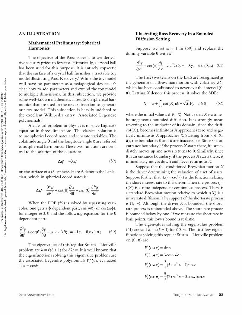
THE JOURNAL OF DERIVATIVES 5520TH ANNIVERSARY ISSUE
AN ILLUSTRATION
Mathematical Preliminary: Spherical Harmonics
The objective of the Ross paper is to use deriva-tive security prices to forecast. Historically, a crystal ball has been used for this purpose. It is entirely copacetic that the surface of a crystal ball furnishes a tractable toy model illustrating Ross Recovery.8 While the toy model will have no parameters as a pedagogical device, it’s clear how to add parameters and extend the toy model to multiple dimensions. In this subsection, we provide some well-known mathematical results on spherical har-monics that are used in the next subsection to generate our toy model. This subsection is heavily indebted to the excellent Wikipedia entry “Associated Legendre polynomials.”
A classical problem in physics is to solve Laplace’s equation in three dimensions. The classical solution is to use spherical coordinates and separate variables. The colatitude angle θ and the longitude angle φ are referred to as spherical harmonics. These two functions are cen-tral to the solution of the equation:
ψ λ= − ψ (59)
on the surface of a (3-)sphere. Here Δ denotes the Lapla-cian, which in spherical coordinates is:
Δ =
∂∂
+∂∂
+∂∂
ψψ
θθ
ψθ
θψ
φ
2
22
2
2cot( ) csc ( )θ
When the PDE (59) is solved by separating vari-ables, one gets a φ dependent part, sin(mφ) or cos(mφ), for integer m ≥ 0 and the following equation for the θ dependent part:
∂∂
+∂∂
− − ,2
22 2y y
+∂
m y yθ
θθ
θ λ= −y θ π∈cot( ) (θ ( ),π,0 (60)
The eigenvalues of this regular Sturm—Liouville problem are λ = �(� + 1) for � ≥ m. It is well known that the eigenfunctions solving this eigenvalue problem are the associated Legendre polynomials Pm
�PP ( )x , evaluated at x = cos θ.
Illustrating Ross Recovery in a Bounded Diffusion Setting
Suppose we set m = 1 in (60) and replace the dummy variable θ with x:
∂∂
+∂∂
− = −2
22y
xx
y
xx y y,cot( ) csc ( )x ( ),λ π∈y x, ( ,0 (61)
The first two terms on the LHS are recognized as the generator of a Brownian motion with volatility 2 , which has been conditioned to never exit the interval (0, π). Letting X denote this process, it solves the SDE:
X x X dsddt
t
s tdsdd+x ,tWW ≥∫0∫∫ 2 0W t,WtWW ≥cot( (62)
where the initial value x ∈ (0, π). Notice that X is a time-homogeneous bounded diffusion. It is strongly mean reverting to the midpoint of its domain, since the drift, cot(X
s), becomes infinite as X approaches zero and nega-
tively infinite as X approaches π. Starting from x ∈ (0, π), the boundaries 0 and π are inaccessible. Since 0 is an entrance boundary, if the process X starts there, it imme-diately moves up and never returns to 0. Similarly, since π is an entrance boundary, if the process X starts there, it immediately moves down and never returns to π.
Suppose that the conditioned Brownian motion X is the driver determining the valuation of a set of assets. Suppose further that r(x) = csc2 (x) is the function relating the short interest rate to this driver. Then the process r
t =
r(Xt) is a time-independent continuous process. There is
a standard Brownian motion relative to which r(Xt) is a
univariate diffusion. The support of the short-rate process is (1, ∞). Although the driver X is bounded, the short-rate process is unbounded above. The short-rate process is bounded below by one. If we measure the short rate in basis points, this lower bound is realistic.
The eigenvalues solving the eigenvalue problem (61) are still λ = �(� + 1) for � ≥ m. The first few eigen-functions solving this regular Sturm—Liouville problem on (0, π) are:
P x
P x x
P
1PP1
2PP1
3PP1
3
(cos )x sin
(cos )x cos sx i
(cos )x
=
=
=33
21
5
23
2
41 35
( c5 )si
(cos ) ( c77 s )
x1)sin
P41(cos 3cos= (7 siss nx
JOD-CARR-CS3.indd 55JOD-CARR-CS3.indd 55 8/23/12 5:34:24 PM8/23/12 5:34:24 PM
The
Jou
rnal
of
Der
ivat
ives
201
2.20
.1:3
8-59
. Dow
nloa
ded
from
ww
w.ii
jour
nals
.com
by
PET
ER
CA
RR
on
09/0
7/12
.It
is il
lega
l to
mak
e un
auth
oriz
ed c
opie
s of
this
art
icle
, for
war
d to
an
unau
thor
ized
use
r or
to p
ost e
lect
roni
cally
with
out P
ublis
her
perm
issi
on.
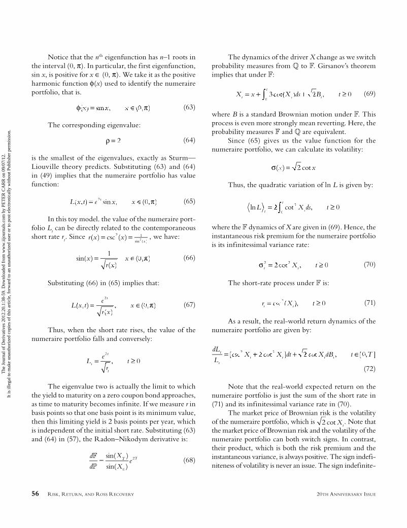
56 RISK, RETURN, AND ROSS RECOVERY 20TH ANNIVERSARY ISSUE
Notice that the nth eigenfunction has n–1 roots in the interval (0, π). In particular, the first eigenfunction, sin x, is positive for x ∈ (0, π). We take it as the positive harmonic function φ(x) used to identify the numeraire portfolio, that is.
φ π) (63)
The corresponding eigenvalue:
ρ = 2 (64)
is the smallest of the eigenvalues, exactly as Sturm—Liouville theory predicts. Substituting (63) and (64) in (49) implies that the numeraire portfolio has value function:
L e t( )x t sin (x ))t x ,2 0 π (65)
In this toy model. the value of the numeraire port-folio L
t can be directly related to the contemporaneous
short rate rt. Since r
x( )x csc ( )x
sin ( )= =csc ( )x2 1
2, we have:
sin( )( )
( )xr(
x= ∈x1 (66)
Substituting (66) in (65) implies that:
Le
r
t
( )x t( )x
( )=)t , ∈x2
(67)
Thus, when the short rate rises, the value of the numeraire portfolio falls and conversely:
Le
rtt
t
tr= , ≥
2
0
The eigenvalue two is actually the limit to which the yield to maturity on a zero coupon bond approaches, as time to maturity becomes infinite. If we measure r in basis points so that one basis point is its minimum value, then this limiting yield is 2 basis points per year, which is independent of the initial short rate. Substituting (63) and (64) in (57), the Radon–Nikodym derivative is:
d
d
X
XeT TFdd
Pdd=
sin( )
sin( )0
2 (68)
The dynamics of the driver X change as we switch probability measures from Q to F. Girsanov’s theorem implies that under F:
X x d B tt
t
s t+x ,BtB ≥∫0∫∫ 2dsdddsddX3 0cot( (69)
where B is a standard Brownian motion under F. This process is even more strongly mean reverting. Here, the probability measures F and Q are equivalent.
Since (65) gives us the value function for the numeraire portfolio, we can calculate its volatility:
σ( ) tx) cot2
Thus, the quadratic variation of ln L is given by:
lnL dt
t
s ,s ≥∫∫ 0Xcot ds t,cot Xcot ds ≥2∫0∫∫2
where the F dynamics of X are given in (69). Hence, the instantaneous risk premium for the numeraire portfolio is its infinitessimal variance rate:
σt t2 2 0X t2 2= ,t2 tXt ≥ (70)
The short-rate process under F is:
r tt tr , ≥)t( )XXtX2 0 (71)
As a result, the real-world return dynamics of the numeraire portfolio are given by:
dL
Ldt d Tt
tt t t tX= + ,[csc ]t ] t [X dB tt t ,X dBt tdB ∈ ]2 2XX 2dt +]XtX 0
(72)
Note that the real-world expected return on the numeraire portfolio is just the sum of the short rate in (71) and its infinitessimal variance rate in (70).
The market price of Brownian risk is the volatility of the numeraire portfolio, which is 2 cot Xt
. Note that the market price of Brownian risk and the volatility of the numeraire portfolio can both switch signs. In contrast, their product, which is both the risk premium and the instantaneous variance, is always positive. The sign indefi-niteness of volatility is never an issue. The sign indefinite-
JOD-CARR-CS3.indd 56JOD-CARR-CS3.indd 56 8/23/12 5:34:24 PM8/23/12 5:34:24 PM
The
Jou
rnal
of
Der
ivat
ives
201
2.20
.1:3
8-59
. Dow
nloa
ded
from
ww
w.ii
jour
nals
.com
by
PET
ER
CA
RR
on
09/0
7/12
.It
is il
lega
l to
mak
e un
auth
oriz
ed c
opie
s of
this
art
icle
, for
war
d to
an
unau
thor
ized
use
r or
to p
ost e
lect
roni
cally
with
out P
ublis
her
perm
issi
on.

THE JOURNAL OF DERIVATIVES 5720TH ANNIVERSARY ISSUE
ness of the risk premium is also not an issue, since X is not the price of a traded asset.
In this toy model, the dynamics of the ith spot price S
it under F are:
dS X t Xx
X dtit i t ti t
t,XtX= +∂ ,Si
∂
+
[ i[ (SSi ))tt ,XtXcot ]Xt
2 2 2
∂ ,∂∂∂
,x
di tt
),tt [ ],T,2 , ∈dB t ∈t [ (73)
SUMMARY AND FUTURE RESEARCH
In this article, we reviewed Ross’s derivation of his Theorems 1 and 2. We then proposed an alternative preference-free way to derive the same financial con-clusion. Our approach is based on imposing stationarity on the real-world dynamics of the numeraire portfolio when it is driven by a bounded diffusion. We illus-trated our approach for gazing into crystal balls by using spherical harmonics.
We suggest the following extensions for future research. First, it would be straightforward to extend this work to two or more driving state variables. So long as each univariate Sturm—Liouille problem is regular, we have uniqueness of the positive eigenfunction. Second, it would be interesting to explore whether Ross recovery is possible on unbounded domains. We know of an example on an unbounded domain for which the uniqueness of positive eigenfunctions fails when the point spectrum is not countable. We also know of an example on an unbounded domain for which we have uniqueness of positive func-tions and the point spectrum happens to be countable. We conjecture that the uniqueness of positive eigenfunc-tions succeeds on unbounded domains if we restrict the function space in some way (e.g., bounded continuous functions), so that the point spectrum becomes count-able. Third, it would be interesting to explore the extent to which Ross’s conclusions survive when the driving process X is generalized into a semi-martingale. Dropping the Markovian condition would mean that one is now searching for the three characteristics of a semi-martingale under F, given that they are known under Q. Methods used to prove the second fundamental theorem of asset pricing should be useful in proving uniqueness. Finally, it would be interesting to explore what restrictions on F can be obtained when markets are incomplete.
Clearly, Ross’s paper and this tweak of it present merely the theoretical foundations for the idea that the separation of variables can be used to separate beliefs from preferences. Much work remains to be done on the implementation and testing phase. In the interest of brevity, theoretical extensions, implementation strate-gies, test designs, and empirical results are best left for future research.
ENDNOTES
The views repesented herein are the authors’ own views and do not necessarily represent the views of Morgan Stanley or its aff iliates and are not a product of Morgan Stanley research.
We are grateful to Aswath Damodoran, Darrell Duffie, Phil Dybvig, Bruno Dupire, Travis Fisher, Bjorn Flesaker, Gabor Fath, Benjamin Forestier, Will Goetzmann, Alan Moreira, Sergey Myagchilov, Steve Shreve, Bruce Tuckman, and especially, Steve Ross, Kevin Atteson, Steve Figlewski, and Zsolt Bihary for their comments. They are not responsible for any errors.
1Long proved this result in a sufficiently regular multi-variate diffusion context. Becherer [2001] extends the result to the unbounded semi-martingale setting.
2To be precise, the market price of Brownian risk is the signed instantaneous lognormal volatility of the numeraire portfolio.
3The observant reader will notice the careful financial engineering that went into matching our equation number with Ross.
4When we consider that (10) is imposed in conjunction with (5), a consequence of this reconciliation is that at the optimum, marginal utility from time one consumption is also invariant to the initial state.
5The structure in (15) has several other surprising impli-cations as well. For example, the bridge laws under F and Q are identical. Furthermore, Küchler [1982] uses (15) to identify a one-parameter exponential family. Finally, if X is a time-homogeneous diffusion, then one can characterize when its time inverse tX
1/t is also a time-homogeneous diffu-
sion. If X is time invertible under F, then under (15), it is also time invertible under Q, and the two time-inverted diffusions are identical (see Lawi [2008]).
6The term “convexity effect” is often used whenever Ef(X) ≠ f(EX); Here, X is in general a random vector, and the function f does not have to be convex or concave. In the authors’ experience, economists frequently attribute these convexity effects to risk aversion, while traders attribute them to “supply and demand.”
JOD-CARR-CS3.indd 57JOD-CARR-CS3.indd 57 8/23/12 5:34:25 PM8/23/12 5:34:25 PM
The
Jou
rnal
of
Der
ivat
ives
201
2.20
.1:3
8-59
. Dow
nloa
ded
from
ww
w.ii
jour
nals
.com
by
PET
ER
CA
RR
on
09/0
7/12
.It
is il
lega
l to
mak
e un
auth
oriz
ed c
opie
s of
this
art
icle
, for
war
d to
an
unau
thor
ized
use
r or
to p
ost e
lect
roni
cally
with
out P
ublis
her
perm
issi
on.

58 RISK, RETURN, AND ROSS RECOVERY 20TH ANNIVERSARY ISSUE
7To the extent that boundary behavior can be imposed on the diffusion X, the corresponding boundary conditions on π are separable.
8Better yet, the final draft of this article was submitted on 22/7 ≈ π.
REFERENCES
Bachelier, L. “Théorie de la Speculation.” Annales Scientifiques de lÉcole Normale Supérieure. Vol. 3, No. 17 (1900), pp. 21-86.
Bajeux-Besnainou, I., and R. Portait. “The Numeraire Port-folio: A New Methodology for Financial Theory.” European Journal of Finance, 3 (1997), pp. 291-309.
Becherer, D. “The Numeraire Portfolio for Unbounded Semimartingales.” Finance & Stochastics, Vol. 5, No. 3 (2001), pp. 327-341.
Bergman, Y. “A Characterization of Self-Financing Port-folio Strategies.” Berkeley Working Paper Number 113, 1981. Available at http://www.haas.berkeley.edu/finance/WP/rpf list.html
Black, F., and M. Scholes. “The Pricing of Options and Cor-porate Liabilities.” Journal of Political Economy, Vol. 81, No. 3 (1973), pp. 637-654.
Carr, P., and S. Nadtochiy. “The Local Variance Gamma Model.” Working paper Oxford University 2012.
Carr, P., H. Géman, D. Madan, and M. Yor. “The Fine Struc-ture of Asset Returns: An Empirical Investigation.” Journal of Business, Vol. 75, No. 2 (2002), pp. 305-322.
Christensen, M. “On the History of the Growth Optimal Portfolio.” 2005. Available at: www.cs.bme.hu/noti/port-folio/articles/history.pdf.
Cox, J. “Notes on Option Pricing I: Constant Elasticity of Variance Diffusions.” Working paper, Stanford University, 1975.
Cox, J., J. Ingersoll, and S. Ross. “A Theory of the Term Structure of Interest Rates” Econometrica, Vol. 53, No. 2 (1985), pp. 385-407.
Dybvig, P., and S.A. Ross. “Arbitrage.” In The New Palgrave Dictionary of Economics, First Edition, edited by J. Eatwell, M. Milgate, and P. Newman, Macmillan and Stockton 1987.
——. “Arbitrage, State Prices and Portfolio Theory.” In Handbook of the Economics of Finance, edited by G.M. Con-stantinedes, and R M. Stultz, Elsevier, 2003.
Eberlein, E., and U. Keller. “Hyperbolic Distributions in Finance.” Bernoulli, 1 (1995), pp. 281-299.
Epstein, L., and S. Zin. “Substitution, Risk Aversion, and the Temporal Behavior of Consumption Growth and Asset Returns I: A Theoretical Framework.” Econometrica, 57 (1989) pp. 937-969.
Géman H., N. El Karoui, and J.C. Rochet. “Changes of Numeraire, Changes of Probability Measures and Pricing of Options.” Journal of Applied Probability, 32 (1995) pp. 443-458.
Hansen, L., and J. Scheinkman. “Long-Term Risk: An Operator Approach.” Econometrica, Vol. 77, No. 1 (2009) pp. 177-234.
Hansen, L. and K. Singleton. “Stochastic Consumption, Risk Aversion, and the Temporal Behavior of Asset Returns.” The Journal of Political Economy, Vol. 91, No. 2 (1983), pp. 249-265.
Heston, S. “A Closed-Form Solution for Options with Sto-chastic Volatility with Applications to Bond and Currency Options.” The Review of Financial Studies, Vol. 6, No. 2 (1993), pp. 327-343.
Hunt, P., J. Kennedy, and A. Pelsser. “Markov-Functional Interest Rate Models.” Finance and Stochastics, Vol. 4 No. 4, (2000), pp. 391-408.
Kelly, J. “A New Interpretation of Information Rate.” Bell System Technical Journal, 35 (1956), pp. 917-926.
Kou, S. “A Jump-Diffusion Model for Option Pricing.” Man-agement Science, Vol. 48, No. 8 (2002), pp. 1086-1101.
Kreps, D., and E. Porteus. “Temporal Resolution of Uncer-tainty and Dynamic Choice Theory.” Econometrica, Vol. 46, No. 1 (1978), pp. 185-200.
Küchler, U. “On Exponential Families of Markov Processes, Part 1: General Results.” Math. Operationsforschung Statist., Ser. Statistics, 13 (1982), pp. 57-69.
Latané, H. “Criteria for Choice Among Risky Ventures.” Journal of Political Economy, 38 (1959), pp. 145-155.
JOD-CARR-CS3.indd 58JOD-CARR-CS3.indd 58 8/23/12 5:34:25 PM8/23/12 5:34:25 PM
The
Jou
rnal
of
Der
ivat
ives
201
2.20
.1:3
8-59
. Dow
nloa
ded
from
ww
w.ii
jour
nals
.com
by
PET
ER
CA
RR
on
09/0
7/12
.It
is il
lega
l to
mak
e un
auth
oriz
ed c
opie
s of
this
art
icle
, for
war
d to
an
unau
thor
ized
use
r or
to p
ost e
lect
roni
cally
with
out P
ublis
her
perm
issi
on.

THE JOURNAL OF DERIVATIVES 5920TH ANNIVERSARY ISSUE
Lawi, S. “Towards a Characterization of Markov Processes Enjoying the Time-Inversion Property.” 2008. Available at http://arxiv.org/pdf/math/0506013.pdf.
Long, J. “The Numeraire Portfolio.” Journal of Financial Economics, 26 (1990), pp. 29-69.
Mehra, R., and E. Prescott. “The Equity Premium: A Puzzle.” Journal of Monetary Economics, Vol. 15, No. 2 (1985), pp. 145-161.
Merton, R. “Option Pricing When Underlying Stock Returns Are Discontinuous.” Journal of Financial Economics, 3 (1976), pp. 125-144.
Meyer, C. Matrix Analysis and Applied Linear Algebra, SIAM, 2000.
Mongin, P. “The Paradox of The Bayesian Experts and State-Dependent Utility Theory.” THEMA Working papers 97-15, THEMA (Theorie Economique, Modélization et Applica-tions), Université de Cergy-Pontoise, 1997.
Platen, E., and H. Bühlmann, “A Discrete Time Benchmark Approach for Finance and Insurance.” Astin Bulletin, Vol. 2, No. 33, 2003.
Platen, E. “On The Role of The Growth Optimal Portfolio in Finance.” Australian Economic Papers, Vol. 44, No. 4 (2005), pp. 365-388.
——. “Diversif ied Portfolios with Jumps in a Benchmark Framework.” Asia-Pacific Financial Markets, Vol. 11, No. 1 (2005), pp. 1-22.
——. “A Benchmark Approach to Finance.” Mathematical Finance, 16 (2006), pp. 131-151.
Platen, E., and D. Heath. A Benchmark Approach to Quantitative Finance. Springer Finance, 2007.
Ross, S.A. “The Recovery Theorem.” Working paper Sept. 10, 2011 forthcoming in Journal of Finance. Available at: http://mitsloan.mit.edu/finance/pdf/Ross-20120109.pdf.
Vasicek, O. “An Equilibrium Characterization of the Term Structure.” Journal of Financial Economics, Vol. 5. No. 2 (1977), pp. 177-188.
Wikipedia, Von Neumann-Morgenstern utility the-orem, available at: http://en.wikipedia.org/wiki/Von_Neumann%E2%80%93Moregensterm_utility_theorem (as of July 22, 2012, 15:55 GMT)
Wikipedia, Perron—Frobenius theorem, available at: http://en.wikipedia.org/wiki/Perron%E2%80%93Frobenius_the-orem (as of July 22, 2012, 13:37 GMT).
Wikipedia, Sturm—Liouville theory, available at: http://en.wikipedia.org/wiki/Sturm (as of July 22, 2012, 13:36 GMT).
Wikipedia, Associated Legendre polynomials, available at: http://en.wikipedia.org/wiki/Associated_Legendre_poly-nomials (as of July 22, 2012, 13:41 GMT
To order reprints of this article, please contact Dewey Palmieri at [email protected] or 212-224-3675.
JOD-CARR-CS3.indd 59JOD-CARR-CS3.indd 59 8/23/12 5:34:25 PM8/23/12 5:34:25 PM
The
Jou
rnal
of
Der
ivat
ives
201
2.20
.1:3
8-59
. Dow
nloa
ded
from
ww
w.ii
jour
nals
.com
by
PET
ER
CA
RR
on
09/0
7/12
.It
is il
lega
l to
mak
e un
auth
oriz
ed c
opie
s of
this
art
icle
, for
war
d to
an
unau
thor
ized
use
r or
to p
ost e
lect
roni
cally
with
out P
ublis
her
perm
issi
on.