©N

atixi

s 2

006

Risk Models and Model Risk

Michel CrouhyNATIXIS Corporate and Investment Bank

FederalFederal Reserve Bank of Chicago Reserve Bank of Chicago –– EuropeanEuropean Central BankCentral Bank

EleventhEleventh AnnualAnnual International International BankingBanking ConferenceConference: Implications : Implications

for Public Policyfor Public Policy

The The CreditCredit MarketMarket TurmoilTurmoil of 2007of 2007--0808September 25-26, 2008

2

Agenda

I. Introduction

II. What went wrong in risk modeling

III. Lessons from this fiasco

IV. Appendix: Need for “second generation” pricing

models for credit derivatives

Presentation partly based on M. Crouhy, R. Jarrow and S. Turnbull: The

Subprime Crisis, Journal of Derivatives, Fall 2008, 1-30.

3

I. Introduction

4

� The current crisis was an accident waiting to happen. The

trigger was a series of events that striked out of the blue:

� In June 2007, attempt by Bear Sterns to bail out two hedge funds

hurt by subprimee mortgage losses – then, attempt by Merrill Lynch

to liquidate some of the funds’ assets revealed how illiquid the

market for such securities has become.

� In July, first bailout by German regulators of IKB.

� In July also, BNP Paribas froze three investment funds with assets of

2 billion euros because the bank could not value the subprime assets

in the funds.

� It seems that all of a sudden the market realized that MBSs,

CDOs of ABS and other structured products were mispriced

Introduction

5

As a consequence, during July and August 2007, lenders and investors

began to worry about risk in mortgage-related securities. This led to

problems with information and problems with liquidity that helped cause the

markets for important securities to "freeze up“ and models to fall apart.

� Information problems

� Inadequate information about the underlying mortgage loans and the

borrowers, especially for subprime mortgages and affordability products (“liar

loans”).

� Loss of confidence in the accuracy of credit ratings from Moody's and Standard and Poor's.

� Market prices became unavailable or unrealistic for many securities, including those rated AAA.

� Lack of knowledge about what positions and liabilities the major banks and other players had.

and…

Introduction

6

…

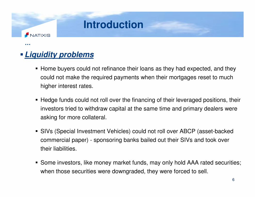
�Liquidity problems

� Home buyers could not refinance their loans as they had expected, and they

could not make the required payments when their mortgages reset to much

higher interest rates.

� Hedge funds could not roll over the financing of their leveraged positions, their

investors tried to withdraw capital at the same time and primary dealers were

asking for more collateral.

� SIVs (Special Investment Vehicles) could not roll over ABCP (asset-backed

commercial paper) - sponsoring banks bailed out their SIVs and took over

their liabilities.

� Some investors, like money market funds, may only hold AAA rated securities;

when those securities were downgraded, they were forced to sell.

Introduction

7

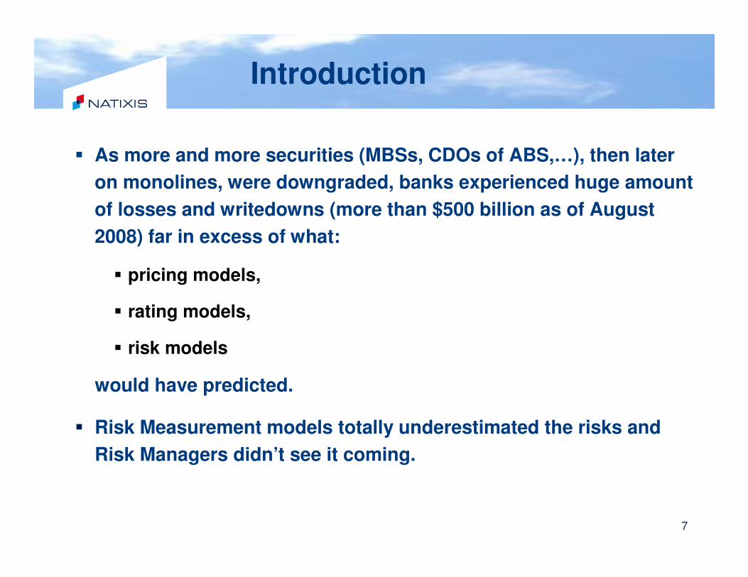
Introduction

� As more and more securities (MBSs, CDOs of ABS,…), then later

on monolines, were downgraded, banks experienced huge amount

of losses and writedowns (more than $500 billion as of August

2008) far in excess of what:

� pricing models,

� rating models,

� risk models

would have predicted.

� Risk Measurement models totally underestimated the risks and

Risk Managers didn’t see it coming.

8

II. What went wrong in risk modeling

9

� “Cliff” effect or non-linearities in the risk of subprime

CDO tranches

� Perhaps one of the biggest failing in the crisis was the failure to

understand the binary (zero-one) nature of mortgage CDOs.

� The assets of a mortgage related CDO were subprime asset backed

bonds. These bonds were themselves tranches on a pool of individual

subprime mortgages. The typical CDO had pools of mortgage backed

bonds rated double B to double A, average triple B.

� Average attachment point for the MB tranches was between 3 to 5% and

the width was very thin from 2.5 to 4%. Assuming a recovery rate of 50%

and a default rate of 20%, a realistic number in the current environment,

then it was to be expected that triple B tranches would be hit.

10

In the current downturn in the housing market and a recessionaryeconomic environment, if one triple B tranche is hit, then it is likely that other triple B tranches will be hit during the same period, especially given the thin width of the tranches.

Collateral Pool:

Subprime

mortgages

AB Bonds

Triple B

bonds

Collateral Pool:

Triple B bonds

CDO

Super

senior

tranches

Either the cumulative default of the subprime mortgages keeps the MB bonds untouched and the super senior tranches will not incur losses, or the default rate wipes out the bonds and the super senior tranches.

11

� Lack of data and inability to calibrate the models

� No history

� Regime change ignored by rating agencies, monolines and structurers in

risk assessment and pricing

12

III. Lessons from this fiasco

13

1.1. CDO CDO tranchestranches are different from corporate are different from corporate

bondsbonds ::It is therefore necessary to model:

1. the cash flows generated by the assets in the collateral pool.

2. prepayments

3. default dependence among the assets

4. how the covariates that explain default by the assets varies over the life

of the structure

5. the waterfall structure of the CDO

The use of well understood assets, such as corporate bonds, as

proxies for the risk of CDO tranches led to mistakes and under-

appreciation of risk.

14

2.2. Check the quality of the raw dataCheck the quality of the raw data

It is essential to perform due diligence on the raw data – neither the rating

agencies nor the banks which structured the CDOs have done it.

(The situation is analogous to an accountant accepting at face value the figures

given to them - no auditing function)

15

3.3. A major source of model risk is the accuracy A major source of model risk is the accuracy

of the key parameters in the valuation of a of the key parameters in the valuation of a

CDO:CDO:

Need to calibrate “forward looking” PDs, LGDs, default

correlations, prepayment rates.

� PDs:

For CDOs we can extract the term structure of PDs from the term structure

of CDSs (assuming some recovery rate).

But for MBSs there is only one maturity – the maturity of the bond.

16

� LGDs:

For mortgages, LGDs depend more than for corporates on the state of the

economy and of the housing market at the time of default.

� Default correlations:

Clearly, there are at least two regimes:

� Normal markets (20%)

� « crisis » regime where correlation jump to a level close to 1 (at

least in some geographic areas with similar socio-professional

characteristics)

17

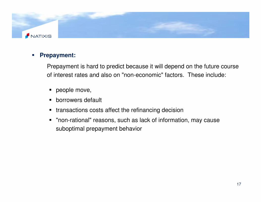
� Prepayment:

Prepayment is hard to predict because it will depend on the future course

of interest rates and also on "non-economic" factors. These include:

� people move,

� borrowers default

� transactions costs affect the refinancing decision

� "non-rational" reasons, such as lack of information, may cause

suboptimal prepayment behavior

18

4.4. In a market that can produce unprecedented price In a market that can produce unprecedented price

moves and significant tail risk:moves and significant tail risk:

� Risk assessment cannot rely on a single risk metric, i.e., VaR

� At least, there is a need to complement traditional risk measures by well

designed, consistent, stress testing and scenario analysis that include

business cycle stresses as well as event specific “tail risks”.

Ensure that the methodology identify and takes into account:

- concentration risk

- correlation risk

- liquidity risk

and covers on-balance sheet as well as off-balance sheet assets.

19

5.5. Pricing models should be Pricing models should be backtestedbacktested..:..:

� …not only, by analyzing the effectiveness of the hedges driven from

the Greeks,

� but also, by explaining the P&L:

Ensure that there is enough granularity in the calibration of the risk

factors to capture the variations of the P&L.

Any material discrepancy between the actual P&L and the P&L

explained by the changes in the risk factors will demonstrate possible

deficiencies in the approach.

20

6.6. Do not neglect Do not neglect ““wrong way correlation riskwrong way correlation risk””::

In the light of what happened with the monolines it is important to

account for the risk that the deterioration of the quality of the assets is

concomitant with a significant increase in the risk of default of the

counterparty.

21

7.7. Need for Need for ““second generationsecond generation”” pricing models pricing models

for credit derivatives:for credit derivatives:

Need to move away from the first generation “Gaussian copula”

model to more robust “second generation” pricing models.

22

IV. Appendix:

Need for “second generation”

pricing models for credit

derivatives

23

IV.1 Standard model for pricing CDO tranches is the

single-factor Gaussian Copula model

Pros: Price quotes with one parameter: base correlation

Cons: Copula models have many shortcomings:

� They are unable to reproduce implied correlations for quoted tranches in a

simple manner

� They are static models which are only good for single-period instruments,

such as CDO tranches, whose prices depend only on marginal distributions

for a series of dates,

� There is no dynamics for spreads and therefore cannot price forward

starting tranches, options on tranches and leveraged super-senior tranches

� Even if you don’t need a dynamic model of the evolution of spreads to price

a CDO tranche, deltas with respect to CDS computed under Copula models

are inconsistent since they do not contain spread risk

24

� Base Correlation Problems with the Gaussian

Copula Model:

� Base Correlation skew: Gauss correlations have a strong slope

� Base Correlation skew leads to interpolation “noise”: thin-tranche arb, bespoke noise

� Credit crisis ���� 100% correlations

� Wide portfolio dispersion exacerbates problems

� Cannot calibrate super-senior tranches

25

� Some Extensions of the Copula Model:

1.Lévy processes

Rational: Credit market events are very shock driven – no smooth behavior

of credit spreads. A CDS, a credit index can jump 20% in a day. It is

then important to model jumps and extreme events.

Gamma model: Main features:

� Downside tail unbounded / upside bounded

� Greater weight in downside tail

26

Base Correlation Results

ITRAXX 5Y: Gaussian 2007-2008

Gaussian Copula: Base Correlations: ITRAXX

0%

10%

20%

30%

40%

50%

60%

70%

80%

90%

100%

8-J

an-0

7

8-M

ar-

07

8-M

ay-0

7

8-J

ul-07

8-S

ep-0

7

8-N

ov-0

7

8-J

an-0

8

8-M

ar-

08

6% 9%

12% 22%

3%

27

Base Correlation Results

ITRAXX 5Y: Gamma

Gamma Copula: Base Correlations: ITRAXX

0%

10%

20%

30%

40%

50%

60%

70%

80%

90%

100%

8-J

an-0

7

8-M

ar-

07

8-M

ay-0

7

8-J

ul-07

8-S

ep-0

7

8-N

ov-0

7

8-J

an-0

8

8-M

ar-

08

6% 9%

12% 22%

3%

28

Base Correlations 2007-2008

CDX 5Y: Gaussian

Gaussian Copula: Base Correlations: CDX.IG

0%

10%

20%

30%

40%

50%

60%

70%

80%

90%

100%

8-J

an-0

7

8-M

ar-

07

8-M

ay-0

7

8-J

ul-07

8-S

ep-0

7

8-N

ov-0

7

8-J

an-0

8

8-M

ar-

08

7% 10%

15% 30%

3%

29

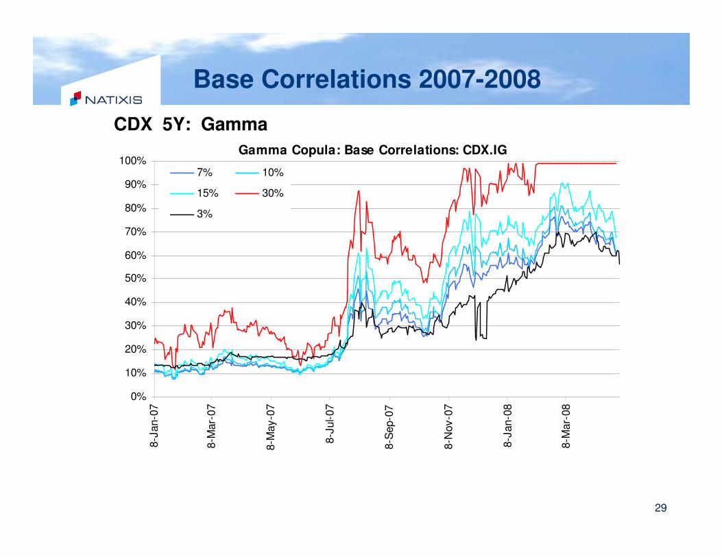
Base Correlations 2007-2008

CDX 5Y: Gamma

Gamma Copula: Base Correlations: CDX.IG

0%

10%

20%

30%

40%

50%

60%

70%

80%

90%

100%8-J

an-0

7

8-M

ar-

07

8-M

ay-0

7

8-J

ul-07

8-S

ep-0

7

8-N

ov-0

7

8-J

an-0

8

8-M

ar-

08

7% 10%

15% 30%

3%

30

Base Correlations 2007-2008

Good news:

� GAMMA base correlation skew is consistently flatter

� Itraxx gamma skew is extremely flat

� Qualitative features of results hold for 5Y, 7Y, 10Y

Bad news:

� CDX – senior correlation still > 99%

Other news:

� Gamma correlation changes more rapidly from day to day

31

� Some Extensions of the Copula Model (Cont.):

2. Stochastic Recovery (Krekel, 2008)

� Choose a recovery distribution unconditional for each issuer

� The variable which drives issuer default also drives the value of loss given default LGD=1-R

� Conditional default rates are positively linked to LGD

32

Choose a Recovery Distribution

Input Recovery Distribution

0

0.1

0.2

0.3

0.4

0.5

0% 20% 40% 60% 80%

WE

IGH

T

Input Recovery Distribution

0

0.1

0.2

0.3

0.4

0.5

0% 20% 40% 60% 80%

WE

IGH

TSR1: Mean 40%, skewed SR2: Mean 40%, greater deviation

Keep in mind: with all weight at 40%, becomes static recovery

33

How the Model Works: Default-Recovery Triggers

� Issuer m defaults before time T if the variable A(m,T) is below a default threshold K0(m,T)

� The realized recovery of issuer m depends on a set of sub-thresholds K1, K2, …

Gaussian model

Cumu default prob : 40%

Choose SR2 (uniform recovery weights)

34

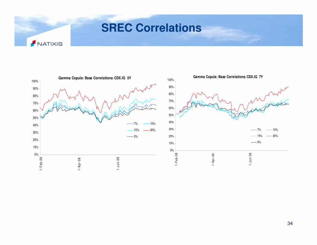
SREC Correlations

Gamma Copula: Base Correlations: CDX.IG 5Y

0%

10%

20%

30%

40%

50%

60%

70%

80%

90%

100%

1-F

eb

-08

1-A

pr-

08

1-J

un

-08

7% 10%

15% 30%

3%

Gamma Copula: Base Correlations: CDX.IG 7Y

0%

10%

20%

30%

40%

50%

60%

70%

80%

90%

100%

1-F

eb

-08

1-A

pr-

08

1-J

un

-08

7% 10%

15% 30%

3%

35

Some issues:

� Gamma copula deltas are noisy

� Analyze the effects on bespoke pricing

� Stochastic Recovery slows down the model:

It would be useful to find efficient approximations in computing deltas

36

IV.2 Many dynamic models have been proposed in

the literature but very few have actually reached

the implementation stage

1. Multi-name default barrier models: Black & Cox

(1976), Hull-White (2001, 2004), Zhou (2002)

� Use the representation of default time as first exit from a barrier

of a state process

� Cons:

� Complex formulas even defaultable discount factors

� Computation of CDO spreads computationally intensive (Monte-

Carlo)

37

2. Random intensity models in the spirit of Duffie &

Garleanu (2001)

� Introduce randomness in spreads by introducing random default

intensities

� Choose random intensity process such as to obtain simple

expressions for conditional default probabilities, e.g., affine

processes

� Pros:

� Closed form expressions for CDS spreads and allow for calibration of

parameters to CDS curves

� Cons:

� Pricing of multiname products done by Monte-Carlo and

computationally intensive

� Calibration to CDO tranche quotes not simple

38

3. Approaches based on portfolio losses

Bottom-up approach

� Calibrate implied default probabilities for portfolio

components to credit default swap term structures

� Add extra ingredient (copula or factor structure) to

obtain joint distribution of default times F(t1,…tn) (n-

dimentional probability distribution)

� Use numerical procedure to compute the risk-neutral

distribution of portfolio loss Lt from F: recursion

methods, FFT, quadrature, Monte-Carlo,…

� Imply correlation parameters from tranche spreads

39

Approaches based on portfolio losses (cont.)

The top-down approach

The idea: view portfolio credit derivatives as options on the total portfolio loss Lt and build a pricing model based on the risk-neutral/market-implied dynamics of Lt

� Approach proposed by Schonbucher which models directly the term-structure of conditional distribution of the total portfolio

loss

Pros:

� Calibration to initial “base correlation skew” is automatic

� Standardized tranches are calibrated so model prices are

consistent with tranche-based hedging

� Provide a joint model for spread and default risk

� No Copulas

40

� Approach proposed by Schonbucher (Cont.)

Cons:

� At present: Just a framework – specification needs to be done

� No deltas / sensitivities to individual names

� Applicable to indices only, not to bespoke portfolios.

� Approach in the spirit of Giesecke & Goldberg where you model the spot loss process Lt

� The portfolio loss process is specified directly in terms of an intensity and a distribution for the loss at an event

� The complete loss surface is described by one set of parameters, and so is the term structure of index and tranche spreads for all attachment points

� Analytical and simulation methods are available to efficiently calculate credit derivative prices

� Single name hedges are generated by thinning the loss process