Risk maps for evaluation of

water-quality monitoring

requirements in England & Wales

Groundwater Programme

Commissioned Report CR/20/030

BRITISH GEOLOGICAL SURVEY

GROUNDWATER PROGRAMME

COMMISSIONED REPORT CR/20/030

The National Grid and other

Ordnance Survey data © Crown Copyright and database rights

2020. Ordnance Survey Licence No. 100021290 EUL.

Keywords

Drinking water, hazard, regulation

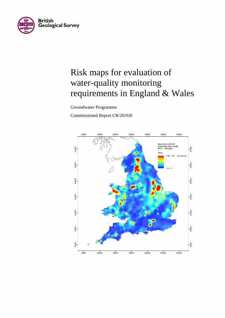
Front cover

Map showing expected value of

aluminium in groundwater, England & Wales.

Bibliographical reference

BEARCOCK, J.M., MILNE, C.J.,

Marchant, B.P., Cartwright, C.E.,

Cave, M.R. and Smedley, P.L. 2020.

Risk maps for evaluation of

water-quality monitoring requirements in England &

Wales. British Geological Survey

Commissioned Report,

CR/20/030. 50 pp.

Copyright in materials derived

from the British Geological Survey’s work is owned by

UK Research and Innovation

(UKRI) and/or the authority that commissioned the work. You

may not copy or adapt this

publication without first obtaining permission. Contact the

BGS Intellectual Property Rights Section, British Geological

Survey, Keyworth,

e-mail ipr@bgs.ac.uk. You may quote extracts of a reasonable

length without prior permission,

provided a full acknowledgement is given of the source of the

extract.

Maps and diagrams in this book

use topography based on

Ordnance Survey mapping.

Risk maps for evaluation of

water-quality monitoring

requirements in England & Wales

J. M. Bearcock, C. J. Milne, B. P. Marchant, C. E. Cartwright, M.

R. Cave and P. L. Smedley

© UKRI 2020. All rights reserved Keyworth, Nottingham British Geological Survey 2020

The full range of our publications is available from BGS

shops at Nottingham, Edinburgh, London and Cardiff (Welsh

publications only) see contact details below or shop online at

www.geologyshop.com

The London Information Office also maintains a reference

collection of BGS publications, including maps, for consultation.

We publish an annual catalogue of our maps and other publications;

this catalogue is available online or from any of the BGS shops.

The British Geological Survey carries out the geological survey of

Great Britain and Northern Ireland (the latter as an agency service

for the government of Northern Ireland), and of the surrounding

continental shelf, as well as basic research projects. It also

undertakes programmes of technical aid in geology in developing

countries.

The British Geological Survey is a component body of UK Research

and Innovation.

British Geological Survey offices

Environmental Science Centre, Keyworth, Nottingham

NG12 5GG

Tel 0115 936 3100

BGS Central Enquiries Desk

Tel 0115 936 3143

email enquiries@bgs.ac.uk

BGS Sales

Tel 0115 936 3241

email sales@bgs.ac.uk

The Lyell Centre, Research Avenue South, Edinburgh

EH14 4AP

Tel 0131 667 1000

email scotsales@bgs.ac.uk

Natural History Museum, Cromwell Road, London, SW7 5BD

Tel 020 7589 4090

Tel 020 7942 5344/45 email bgslondon@bgs.ac.uk

Cardiff University, Main Building, Park Place, Cardiff

CF10 3AT

Tel 029 2167 4280

Maclean Building, Crowmarsh Gifford, Wallingford

OX10 8BB

Tel 01491 838800

Geological Survey of Northern Ireland, Department of

Enterprise, Trade & Investment, Dundonald House, Upper

Newtownards Road, Ballymiscaw, Belfast, BT4 3SB

Tel 01232 666595

www.bgs.ac.uk/gsni/

Natural Environment Research Council, Polaris House,

North Star Avenue, Swindon SN2 1EU

Tel 01793 411500 Fax 01793 411501

www.nerc.ac.uk

UK Research and Innovation, Polaris House, Swindon

SN2 1FL

Tel 01793 444000

www.ukri.org

Website www.bgs.ac.uk

Shop online at www.geologyshop.com

BRITISH GEOLOGICAL SURVEY

i

Foreword

This project was commissioned by the Drinking Water Inspectorate (DWI) for the production of

risk maps showing the distributions of inorganic chemicals and a number of physical parameters

listed in the 98/83/EC Directive, for both surface water and groundwater. The work was conducted

under DWI project itt_3641 (24830) between 2018 and 2020.

The BGS project team comprised specialists in hydrogeochemistry, water sampling and laboratory

analysis, database management, GIS, statistics and geostatistics. Jenny Bearcock managed the

project and was responsible for data acquisition, database population, error checking and DWI

liaison; Chris Milne designed and managed the databases; Ben Marchant was responsible for

geostatistical modelling and mapping; Clive Cartwright designed and built the GIS; Mark Cave

carried out exploratory data analysis including time series; and Pauline Smedley directed and

coordinated the project and DWI liaison.

This Commissioned Report outlines the procedures involved in collating, error checking, and

evaluating the water-quality data before map production. Interactive risk maps are supplied in an

associated mxd (ArcGIS) file.

ii

Acknowledgements

We acknowledge the organisations who have provided raw water-quality data for this evaluation.

These organisations are: the Drinking Water Inspectorate (Department for Environment, Food &

Rural Affairs, Defra), together with water companies and local authorities of England and Wales

supplying the primary data; Environment Agency; Natural Resources Wales; UK Centre for

Ecology & Hydrology and the British Geological Survey. The help of staff from these institutes

involved in supplying the data and licensing terms is also gratefully acknowledged.

Thanks are also due to DWI: James Medland for project management and Richard Phillips, Andy

Taylor, Mike Turrell and Peter Marsden for project advice, direction and liaison.

iii

Contents

Foreword ......................................................................................................................................... i

Acknowledgements ........................................................................................................................ ii

Contents ......................................................................................................................................... iii

Summary ........................................................................................................................................ 1

1 Introduction ............................................................................................................................ 2

1.1 Background ..................................................................................................................... 2

1.2 Terms of reference .......................................................................................................... 2

2 Data compilation and structure ............................................................................................ 3

2.1 Selection of parameters .................................................................................................. 3

2.2 Data acquisition .............................................................................................................. 3

2.3 Data structure .................................................................................................................. 5

2.4 Geospatial tagging .......................................................................................................... 7

2.5 Parameters and units ....................................................................................................... 7

2.6 Combined database ......................................................................................................... 9

3 Data cleaning ........................................................................................................................ 10

3.1 Identification errors ...................................................................................................... 10

3.2 Spatial errors ................................................................................................................. 12

3.3 Errors in measurements or results ................................................................................ 13

3.4 Exploratory data analysis .............................................................................................. 15

4 Water-quality mapping ....................................................................................................... 17

4.1 Probabilistic mapping of the water-quality parameters ................................................ 17

4.2 Creation of interactive maps ......................................................................................... 32

5 Mapping appraisal and review ........................................................................................... 34

5.1 Limitations .................................................................................................................... 34

6 Recommendations ................................................................................................................ 37

6.1 Recommendations to evaluate the process ................................................................... 37

6.2 Recommendations to review the process...................................................................... 37

6.3 Recommendations to improve the process ................................................................... 37

References .................................................................................................................................... 39

iv

FIGURES

Figure 2.1 Database entity-relationship structure ........................................................................... 6

Figure 3.1 Cleaned EA data .......................................................................................................... 13

Figure 4.1 Histograms of observed total groundwater aluminium concentrations in µg/L (left)

and transformed units (right). Vertical black lines indicate 30%, 60% and 100% of the PCV.

Vertical red line indicates the modal Environment Agency detection limit within the

dataset ..................................................................................................................................... 22

Figure 4.2 Most recent observation of total groundwater aluminium at each site in normalised

units (left) and variograms of the temporal average of the normalised groundwater

aluminium observations (in red, right) ................................................................................... 23

Figure 4.3 Predictions of total groundwater aluminium concentration in normalised units (left)

and standard error of these predictions (right) ........................................................................ 24

Figure 4.4 Expected concordance correlation between predicted temporal average groundwater

aluminium concentration in normalised units and actual value in normalised units .............. 24

Figure 4.5 Predictions of expected total groundwater aluminium concentration in µg/L (left) and

predicted 95th percentile (right). Colour scales are censored at PCV value of 200 µg/L so

that darkest red indicates prediction greater than or equal to 200 µg/L ................................. 24

Figure 4.6 Most recent observation of total surface water boron at each site in normalised units

(left) and variogram of the normalised groundwater boron observations (right) ................... 25

Figure 4.7 Predictions of total surface water boron concentration in normalised units (left) and

standard error of these predictions (right) .............................................................................. 25

Figure 4.8 Most recent observation of total surface water antimony at each site in normalised

units (left) and variogram of the normalised observations (right) .......................................... 26

Figure 4.9 Locations of measurements of groundwater nickel since 2015 (left) and expected

concordance correlation between predicted temporal average groundwater nickel

concentration in normalised units and actual value in normalised units (right) ..................... 27

Figure 4.10 Predictions of expected groundwater nickel concentration in µg/L (left) and 95th

percentile (right). Colour scales are censored at PCV of 20 µg/L so that darkest red indicates

prediction equal to or greater than 20 µg/L ............................................................................ 27

Figure 4.11 Locations of measurements of surface-water nickel since 2015 (left) and expected

concordance correlation between predicted temporal average groundwater nickel

concentration in normalised units and actual value in normalised units (right) ..................... 28

Figure 4.12 Predictions of expected groundwater nickel concentration in µg/L (left) and 95th

percentile (right). Colour scales are censored at PCV of 20 µg/L so that darkest red indicates

prediction equal to or greater than 20 µg/L ............................................................................ 28

Figure 4.13 Locations of measurements of surface-water nickel in entire dataset (left) and

expected concordance correlation between predicted temporal average groundwater nickel

concentration in normalised units and actual value in normalised units (right) ..................... 31

Figure 4.14 Predictions of expected surface-water nickel concentration in µg/L (left) and

predicted 95th percentile (right) based on all available measurements. Colour scales are

censored at PCV value of 20 µg/L so that darkest red indicates prediction equal to or greater

than 20 µg/L ........................................................................................................................... 32

v

TABLES

Table 1. Parameters included in this study ...................................................................................... 3

Table 2. Codes used to identify datasets and sources ..................................................................... 5

Table 3. Standard parameters dictionary ......................................................................................... 7

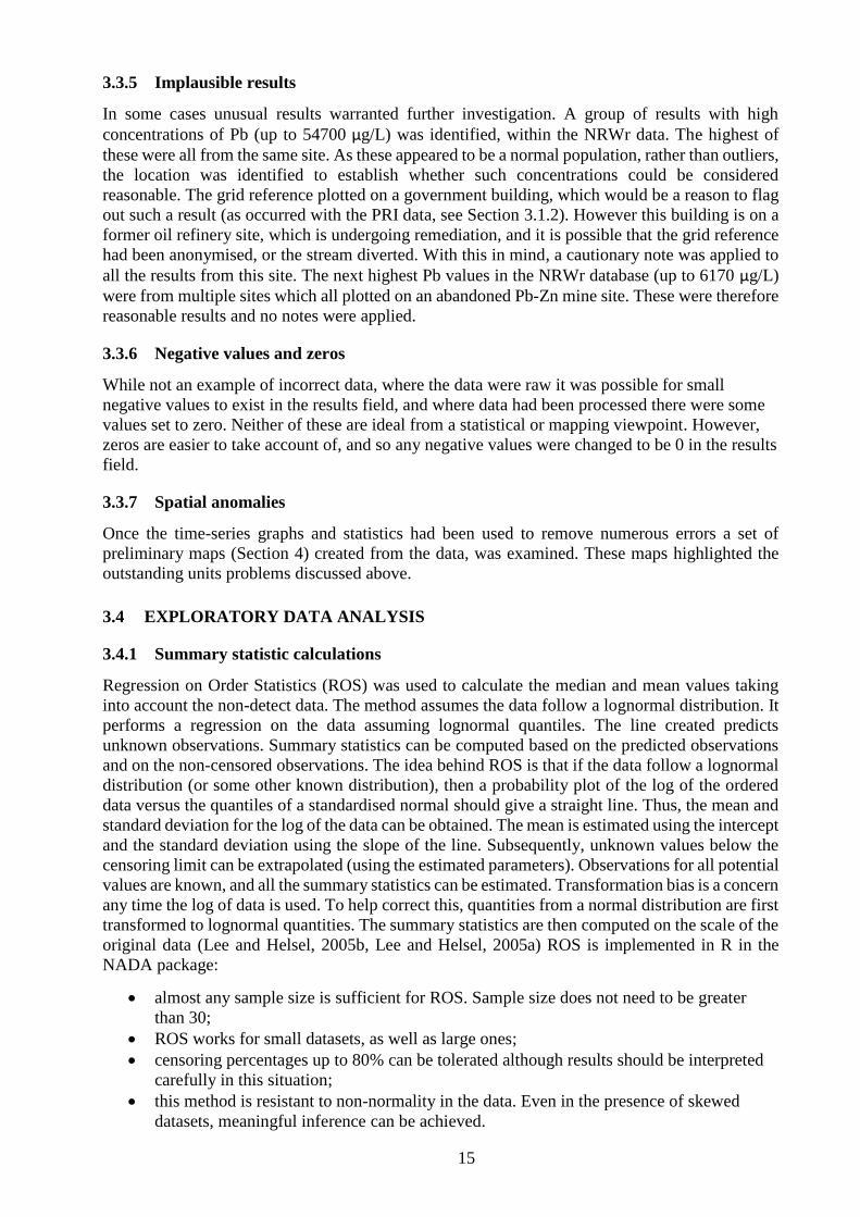
Table 4. Summary of water-quality measurements since January 2015 ....................................... 20

Table 5. Proportion of prediction sites where according to criteria described in the text it is

possible to make an assessment of concentration of a subsequent measurement relative to the

stated threshold ....................................................................................................................... 30

vi

1

Summary

This report details the steps taken in the process of producing risk (hazard) maps for chemical

parameters listed in the European Commission Directive 98/83/EC on the quality of water intended

for human consumption and the national Water Supply (Water Quality) Regulations that

implement the requirements of the directive for drinking water in England and Wales.

Amendments to 98/83/EC set out in Directive 2015/1787 provide the terms for reduced monitoring

requirements by European Member States for drinking water where evidence indicates that water-

quality risk is low. On the basis of the Water Safety Plan approach of the World Health

Organization, DWI requires mapping of available data on raw-water sources in England and Wales

to provide an evaluation of spatial distributions of the listed chemical parameters and their

concentration ranges as evidence of risk for drinking water. An evaluation of temporal variability

was also required to assess evidence for any trends to aid with decision making on future drinking-

water monitoring requirements.

Data for an agreed list of 27 chemical parameters were collated, screened, evaluated and mapped,

with surface water and groundwater being treated separately. This report details the data sources

and steps taken to collate, evaluate, process and map them.

Risk maps produced for individual parameters include expected values and 95th percentiles of

measured values relative to the prescribed concentration or value (PCV) at any given location. The

methodology employed required prediction of the entire statistical distribution of each parameter

at each prediction location so that both expected value and percentile values for each parameter

could be determined. This required the use of a statistical model to represent the variation of the

data. The produced risk maps are produced for water-quality data analysed over the last three

years, in line with the requirements of the 2015/1787 Directive. The correspondence between the

two layers is an indication of the spatial data availability and the strength of correlation between

measurements from nearby sites. The maps are presented in ArcGIS with additional explanatory

layers comprising open-source data for coastline, multiscaled atlases, postcode sectors, place

names, simplified geology, Environment Agency region boundaries and local authority boundaries

as points of reference. The GIS is presented as a separate mxd file.

The maps have inevitable limitations derived from inability to guarantee complete elimination of

errors from the cleaned datasets, paucity of data for some parameters, spatial and temporal

variability of available data for others, variable spreads of surface-water drainage or aquifers,

variable detection limits for some trace elements, and for groundwaters, variable chemistry with

depth, especially for concealed and/or stacked aquifers. Nonetheless, the maps provide an estimate

of the current best-available spatial distributions for parameters for surface water and groundwater

to aid DWI in assessing drinking-water risks and determining monitoring requirements, in line

with Directive 2015/1787. It is anticipated that the maps will be used alongside available site-

specific water-quality monitoring data and site risk assessments for decision making in the context

of the Directive.

Temporal variability of raw water chemical data have also been assessed. As temporal trends vary

significantly spatially for individual parameters and between parameters, recommendations for

timescales of map revision are difficult to make. As a pragmatic recommendation, a mapping

renewal interval on the order of 10 years is considered appropriate. In the case of amendments to

the statutory PCVs in the meantime, remapping is possible using the existing rasters and relating

to the revised threshold values.

2

1 Introduction

1.1 BACKGROUND

European Commission Directive 98/83/EC on the quality of water intended for human

consumption outlines the parameters to be monitored by Member States and the details of

monitoring frequency for compliance points. Water-quality monitoring data indicate that for many

parameters, source types and sample locations, concentrations exceed given thresholds only

occasionally or rarely. Monitoring is costly and so taking steps to reduce monitoring frequency for

such parameters without compromising public health is a major cost-saving incentive. European

Commission Directive 2015/1787 sets out amendments to the 98/83/EC Directive allowing more

flexible monitoring schedules where justified by existing data and risk assessments conducted in

line with the Water Safety Plan approach of the World Health Organization.

EC 2015/1787 (Annex II Part C 5b) details that, in order to reduce the minimum sampling

frequency of a given parameter (excepting E. coli), concentrations obtained from regular

monitoring at representative points over periods of at least 3 years must all be less than 60% of the

parametric value. To remove a parameter from the list to be monitored altogether, the equivalent

observations must all be less than the 30% of the parametric value. The Directive states further

that monitoring of the given parameter may only be reduced or halted if the risk assessment has

confirmed no reasonably anticipated future deterioration of water quality with respect to the

parameter.

Implementing the 2015/1787 Regulations in England & Wales in line with the risk-based Water

Safety Plan approach requires evaluation of raw-water data collected and monitored by water

companies as well as by regulators in compliance with the Water Framework Directive (WFD).

Evaluation and mapping of these data would support the requirements of the Directive and help

decision making on monitoring schedules.

Given the revised specifications, DWI requires the production of a set of risk (hazard) maps for

chemical parameters listed in the 98/83/EC Directive, for surface water and groundwater, in order

to appraise the potential for future reduction in monitoring requirements for both water companies

for public supplies and private water-supply owners, across England & Wales. This report details

a planned approach and methodology to collate, evaluate and map the given parameters as a

framework for implementation for future water-monitoring strategy.

1.2 TERMS OF REFERENCE

The terms of reference defined by DWI for the project were:

Selection of parameters for assessment;

Data gathering of raw water quality and hydrogeological characteristics;

Production of risk maps based on parameter distributions, geological and hydrogeological

characteristics, surface water and groundwater;

Highlighting of the limitations and potential risks from interpretation of the maps;

Recommending frequency of required map updates;

Reporting.

This report is the final step in the sequence of activities outlined above. It details the methodology

used to create the water-quality risk maps. The maps can be accessed interactively using the

associated GIS.

3

2 Data compilation and structure

2.1 SELECTION OF PARAMETERS

All 27 parameters listed in the DWI call for proposals were included in this evaluation. The list is

given in Table 1.

Table 1. Parameters included in this study

Parameter name Parameter

symbol

Unit used in

Regulations

PCV 60% PCV 30%PCV

Aluminium Al µg/L 200 120 60

Arsenic As µg/L 10 6 3

Boron B mg/L 1 0.6 0.3

Cadmium Cd µg/L 5 3 1.5

Chloride Cl mg/L 250 150 75

Cyanide CN µg/L 50 30 15

Colour Colour mg/L Pt-Co

(Hazen)

20 12 6

Conductivity Conductivity µS/cm at 20°C 2500 1500 750

Chromium Cr µg/L 50 30 15

Copper Cu mg/L 2 1.2 0.6

Fluoride F mg/L 1.5 0.9 0.45

Iron Fe µg/L 200 120 60

Gross alpha Gross α Bq/L 0.1 0.06 0.03

Gross beta Gross β Bq/L 1 0.6 0.3

Mercury Hg µg/L 1 0.6 0.3

Manganese Mn µg/L 50 30 15

Sodium Na mg/L 200 120 60

Ammonium NH4 mg/L 0.5 0.3 0.15

Nickel Ni µg/L 20 12 6

Nitrite NO2 mg/L 0.5 0.3 0.15

Nitrate NO3 mg/L 50 30 15

Lead Pb µg/L 10 6 3

pH pH pH units 6.5–9.5

Antimony Sb µg/L 5 3 1.5

Selenium Se µg/L 10 6 3

Total organic carbon TOC mg/L No abnormal change

Turbidity Turbidity NTU 4 2.4 1.2

2.2 DATA ACQUISITION

Water-quality data were obtained from DWI, the Environment Agency, Natural Resources Wales,

British Geological Survey and the UK Centre for Ecology & Hydrology. Each dataset had separate

challenges to check and manage. Relevant licensing information was stored with each dataset, and

a summary table created indicating data holder, dataset name, dataset source organisation, the URL

of the download or contact name, licence number, terms of storage and disposal, any copyright

statement and papers which must be referenced.

Datasets deemed unsuitable or superseded were omitted from further consideration. Each dataset

used is discussed separately below.

4

2.2.1 DWI

Data from DWI originated from two sources: raw water from water company public-water sources,

and water from private supplies taken directly from consumers’ taps, supplied to DWI by local

authorities. As a result, the latter in some cases may unavoidably represent treated water. Absence

of metadata supplied on treatment precluded any evaluation of the dataset in this regard.

One spreadsheet was supplied for each public water company (26 in total), with a summary table

of metadata including translation for the company codes, information regarding mergers of

companies and date range of reported data. A separate spreadsheet was also supplied for each year

of local authorities’ private water-supply data (7 in total), and an explanatory spreadsheet

translated various codes used within the data files. For both public and private water datasets,

unfiltered values were used.

2.2.2 BGS (G-BASE)

The Geochemical Baseline Survey of the Environment (G-BASE) was a long-running BGS

project, which had an annual sampling programme from 1968–2014. Among other sample media,

stream water samples were collected from low-order streams at an average density of one sample

every 1.5 km2. Each site was only sampled once, so provides a snapshot of the geochemistry at a

given time.

The data were downloaded from the BGS’s corporate Geochemistry Database, exported as a single

Excel spreadsheet. The data are usually reported raw (uncensored) with a qualifier used to identify

where a result is below the detection limit. For some analyses, a qualifier identifies where a result

has been set to half detection limits. Analyses were in all cases filtered (0.45 µm).

2.2.3 NRW

The Natural Resources Wales (NRW) data are from the Water Quality Archive, which provides a

central repository for water-quality data. Samples are taken from coastal or estuarine waters, rivers,

lakes, ponds, canals or groundwater. The Water Quality Archive replaced the Environment

Agency’s (EA) Water Information Management System (WIMS) database. Since NRW became a

separate entity from the EA in 2013, the Welsh data have been managed separately.

Data from NRW were split into two separate packages. The first comprised older data, which were

archived as the Historic UK Water Quality Sampling Harmonised Monitoring Scheme (HMS).

These data represent the time period when NRW was a part of the EA (to 2013) and were

downloaded from “Lle”, a geo-portal for Wales developed in partnership between Welsh

government and NRW. The data download comprised an Access database, with normalised data

and lookup information as a series of tables.

The second package represented the more recent data (2013–2017), which have been collected and

collated since NRW became independent. The data were downloaded securely as a spreadsheet in

a flat-file format. Unfiltered analyses were used for data evaluation.

2.2.4 UKCEH

Formed in the year 2000, the Centre for Ecology & Hydrology (CEH) represented the merger of

four Natural Environment Research Council (NERC) research institutes. As of December 2019,

CEH became an independent registered charity and rebranded to the UK Centre for Ecology &

Hydrology (UKCEH). The data obtained from UKCEH represented numerous individual projects

relating to water quality. Almost all the samples were surface water, and each of the datasets

represented smaller projects, in terms of number of samples, spatial extent, and/or timeframe.

These data were identified and downloaded from the UKCEH-hosted Environmental Information

Data Centre (EIDC), or from data.gov.uk.

5

A total of 18 datasets were downloaded, but five were later archived as they were not suitable.

Either there were too few results to merit investment of time to clean and manage, or they

represented a specific event which would not provide representative data (such as monitoring in

response to a pollution event), or the grid references were too heavily restricted to be of any use.

As they all represented separate projects undertaken by different researchers at different times,

each downloaded dataset was different. Some were in crosstab format, others flat-file or

normalised, others were neither truly crosstab nor normalised. Some site information (names and

grid references) appeared in the data spreadsheet within row headings, some in a separate tab. For

other datasets, site information was in a separate spreadsheet, for others it was listed in a Word or

pdf file. The presentation of units was also variable. In some cases, the same parameter could be

referred to in numerous ways between datasets, for example Na, Na mg/L, Sodium, or Sodium

Dissolved. Information on sample form (dissolved/total/acidified) was also inconsistent. The same

parameter could be expressed in different units or within a different form, for example NO3 data

could be presented as NO3 or NO3-N and in units of mg/L, µg/L or meq/L. Analyses selected for

incorporation to the dataset were unfiltered.

2.2.5 EA

Environment Agency (EA) data are usually available from the EA Water Quality Archive via

data.gov.uk. As described above (Section 2.2.3) this archive replaces the WIMS database, and

specifically only the data from sampling points around England are available from this source. The

samples within this dataset can be from coastal or estuarine waters, rivers, lakes, ponds, canals or

groundwater. They are taken for a variety of purposes including compliance assessment,

investigation of specific pollution incidents, or environmental monitoring. All selected analyses

were unfiltered.

During the period of the study assigned to data collection at the start of the project (spring/summer

2018), the data download was not available online. Instead, the EA were contacted directly and

the data were supplied as Access databases.

2.2.6 Other

A literature search was undertaken to try to identify any other available digital datasets. Key words

including groundwater, stream water, surface water, natural water, drinking water, chemistry,

quality, England, Wales, and England and Wales were used to search on Web of Science, Scopus,

and Google Scholar. No suitable additional datasets were found.

2.3 DATA STRUCTURE

At the first stage, each of the datasets obtained from the different sources (above) was prepared

separately owing to differing formats in which they were received. Each dataset was given a short

code to facilitate file-naming consistency during the subsequent stages. NRW data were processed

as two separate datasets because of the two origins. A summary of each dataset code, name, and

data owner is presented in Table 2. Hereafter, these codes will be used to refer to each dataset.

Table 2. Codes used to identify datasets and sources

DataSet

Code Dataset Name

Data

Owner

Code

Data Owner Name

EA Environment Agency Water Quality

Archive EA Environment Agency

NRWo Natural Resources Wales Water Quality

Data (old: Pre-2013) NRW Natural Resources Wales

6

NRWr Natural Resources Wales Water Quality

Data (recent: 2013–2017) NRW Natural Resources Wales

*CEH UK Centre for Ecology & Hydrology

various project datasets UKCEH

Centre for Ecology &

Hydrology

GB G-BASE (Geochemical Baseline Survey

of the Environment) BGS British Geological Survey

PUB Public water supplies DWI Drinking Water Inspectorate

PRI Private water supplies DWI Drinking Water Inspectorate

*For data naming purposes the abbreviation CEH will be used within the database rather than UKCEH.

Preliminary data manipulation was carried out in Microsoft Access, rather than a full SQL-based

relational Database Management System (DBMS, such as Oracle or Microsoft SQL-Server) as the

Access user interface is more agile for rapid and smaller-scale manipulation of the data structure.

At all stages, errors that became apparent were, whenever possible, corrected before continuing.

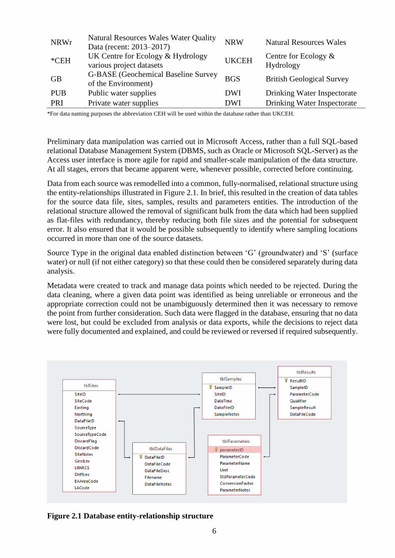
Data from each source was remodelled into a common, fully-normalised, relational structure using

the entity-relationships illustrated in Figure 2.1. In brief, this resulted in the creation of data tables

for the source data file, sites, samples, results and parameters entities. The introduction of the

relational structure allowed the removal of significant bulk from the data which had been supplied

as flat-files with redundancy, thereby reducing both file sizes and the potential for subsequent

error. It also ensured that it would be possible subsequently to identify where sampling locations

occurred in more than one of the source datasets.

Source Type in the original data enabled distinction between ‘G’ (groundwater) and ‘S’ (surface

water) or null (if not either category) so that these could then be considered separately during data

analysis.

Metadata were created to track and manage data points which needed to be rejected. During the

data cleaning, where a given data point was identified as being unreliable or erroneous and the

appropriate correction could not be unambiguously determined then it was necessary to remove

the point from further consideration. Such data were flagged in the database, ensuring that no data

were lost, but could be excluded from analysis or data exports, while the decisions to reject data

were fully documented and explained, and could be reviewed or reversed if required subsequently.

Figure 2.1 Database entity-relationship structure

7

2.4 GEOSPATIAL TAGGING

In order to provide additional spatial information for categorising sites, a number of spatial

attributes were added to the sites tables. Publicly available shapefiles of local authority areas and

EA areas were obtained from data.gov.uk, and added to a GIS project together with the BGS

1:625,000 surface solid geology and surface drift geology maps. The site locations from each

source database were added to the GIS project and for each point an attribute code was extracted

from each shapefile. Each site was therefore assigned codes to identify:

local authority area,

EA area,

solid geology stratigraphy (code from the BGS RCS Lexicon),

solid geology lithology, and

drift geology.

The codes for each of these were recorded back into the databases for each site using fields added

to the Sites tables for the purpose.

2.5 PARAMETERS AND UNITS

The original data sources provided to the project sometimes used different parameter names and/or

measurements units for the same parameters, according to the reporting conventions of the source

organisation or originating laboratory. During the preparation of the databases here the individual

results were retained with their native names and units to maintain traceability. The parameters

table therefore includes fields for a Std Parameter Code and a units Conversion Factor. These fields

provided the means to standardise the results from the disparate sources into a single consistent

dataset for the statistical and spatial analysis.

Table 3. Standard parameters dictionary

StdParamCode StdParamName StdParamUnit PCV

Al-T Aluminium (Total) µg/L 200

As-T Arsenic (Total) µg/L 10

B-T Boron (Total) mg/L 1

Cd-T Cadmium (Total) µg/L 5

Cl Chloride mg/L 250

CN Cyanide µg/L 50

Col-Hazen Colour mg/L Pt-Co 20

Cond-20 Conductivity at 20°C µS/cm 2500

Cr-T Chromium (Total) µg/L 50

Cu-T Copper (Total) mg/L 2

F Fluoride mg/L 1.5

Fe-T Iron (Total) µg/L 200

Gross α Total Gross alpha Bq/L 0.1

Gross β Total Gross beta Bq/L 1

Hg-T Mercury (Total) µg/L 1

Mn-T Manganese (Total) µg/L 50

Na-T Sodium (Total) mg/L 200

NH4 Ammonium mg/L 0.5

Ni-T Nickel (Total) µg/L 20

NO2 Nitrite mg/L 0.5

NO3 Nitrate mg/L 50

Pb-T Lead (Total) µg/L 10

8

pH pH pH units 6.5–9.5

Sb-T Antimony (Total) µg/L 5

Se-T Selenium (Total) µg/L 10

TOC-T Total organic carbon mg/L No abnormal change

Turb-NTU Turbidity in NTU units NTU 4

The standard parameters dictionary (Table 3) which was created therefore contains a short code

and an assigned reporting unit for each of the parameters required under the remit of this study.

The standardised reporting units used for each parameter are those used in the Water Supply

(Water Quality) Regulations 2018 (WSI, 2018).

Table 3 was then used to assign each parameter in the individual databases to a standard parameter.

A conversion factor field was added to ensure that parameters could be converted automatically

into the correct units. While some of the parameters were provided in a variety of different units,

these were usually straightforward to convert to the standard unit. The most common conversions

were mg/L to µg/L, or vice versa. There were a few instances of parameters being reported in

meq/L which were also converted. Less straightforward to convert were various units of

conductivity, colour, and turbidity.

2.5.1 Colour

The standard unit for colour is mg/L Pt-Co, which is equivalent to Hazen units. In the UKCEH

database, 1.5% of colour measurements were reported in nm. As no simple conversion could be

found, results with these units were not used.

2.5.2 Conductivity

Electrical conductivity, the ability of water to conduct an electric current, is typically reported as

specific electrical conductance, or conductance per unit length and unit cross-sectional area at a

specified temperature. The standard unit of measurement is µS/cm and the standard temperature

is 25 °C (Hem, 1992). However, the unit reported in water-quality regulations is conductivity in

µS/cm at 20 °C.

Of the conductivity data collated for this study, 49% of measurements were reported at 20 °C, 28%

were reported at 25 °C, and 23% did not specify which temperature they were recorded at.

The relationship between temperature and conductivity is not linear, which means a simple

conversion factor, as required by the database structure, cannot be applied. However, in the

temperature range of most natural waters (0–30 °C), the degree of nonlinearity is negligible and a

linear equation can be used to represent the relationship between temperature and conductivity:

𝐸𝐶𝑡 = 𝐸𝐶25[1 + 𝑎(𝑡 − 25)]

Where ECt is electrical conductivity at temperature t (°C), EC25 is SEC and a (°C-1) is a temperature

compensation factor (Hayashi, 2004). A variety of compensation factor values are cited in the

literature (see Hayashi, 2004). The compensation factor used in this study (0.0187) was defined

by Hayashi (2004) deduced from the examination of natural waters. This gives a conversion factor

of 0.906 (to 3 significant figures) that has been applied to convert from conductivity reported at

25 °C to that at 20 °C.

Where the temperature of reported measurement has not been given, it is not possible to use the

results any further as it is not known if they were reported at 20 °C, 25 °C, or another temperature.

9

2.5.3 Turbidity

Turbidity is caused by the presence of suspended, colloidal and/or coloured matter and can be

measured in a variety of ways depending on the intended use of turbidity data. As a result, a range

of instruments have been developed to meet the various objectives. While calibrated using the

same standards (formazin), the turbidity measurements these instruments give can differ by factors

of two or more for the same environmental sample (Anderson, 2005).

Historically, units were reported as Jackson Turbidity units (JTU) or Formazin Turbidity Units

(FTU), but neither is still in common use because of lack of precision (JTU), or lack of information

regarding which instrument was used (FTU). It is also currently common for NTU (Nephelometric

Turbidity Unit) to be used as a general turbidity unit. To ensure that turbidity data could be

properly interpreted and used the reporting units have now been standardized to be specific to the

instrument and method type. This has created a large range of units, but it means that users of data

can be sure that comparisons of data over time, between sites, instruments, and studies are valid

(Anderson, 2005). One such unit is NTU, which now has a specific meaning relating to the

particular methodology (Anderson, 2005), but caution must be taken if it is uncertain whether the

unit has been used to describe a specific method or represents a generic unit.

In this study, data have been reported in NTU and FTU. The water-quality standards report

turbidity in NTU. Of the data collated in this study, 18% were reported in FTU. It is unclear

whether the results reported in NTU are also reporting generic turbidity results or a specific

methodology, and this may differ between data sources.

Under certain circumstances NTU is the same as FTU: 1 NTU = 1 FTU measured

nephelometrically (National Water Council Standing Committee of Analysts, 1984). It is uncertain

how each data provider has measured the data. The DWI advised that data reported in NTU should

be combined with data reported in FTU, given that ISO defines the standards noting there is

“numerical equivalence of the units NTU and formazin nephelometric unit (FNU)” (ISO, 2016).

2.6 COMBINED DATABASE

The aggregate volume of data collected by the project was too large to be handled using a desktop

database such as Microsoft Access. The cleaned data from the various sources were therefore

combined into a single database using SQL Server. To retain the ability to edit and manage

individual datasets separately, the data were loaded onto the server as distinct sets of tables for

each source. A set of data views was then constructed within SQL, using the relational structure

described previously, to combine all of the sources together into a single dataset.

Prior to combining the databases the site, sample, and parameter IDs from each source database

were prefixed with the short code of the source database. This guaranteed that every record had a

truly unique primary identifier.

The overall structure provided strong data management, with robust access control and security,

and automated backup. The normalised relational structure helped to ensure good version and

change control as individual data were stored once in their source tables, and any changes or

corrections to data would be immediately reflected in any derived views.

The cleaned and combined database was very substantial, containing records for:

107,000 unique sites

3.9 million samples

22.2 million measurement results

of which approximately 15.0 million were for the list of standard parameters

and occupying about 9 GB of filespace on the server.

10

3 Data cleaning

The process of data preparation was much more prolonged than first envisaged because of the need

to correct for inconsistencies and errors within the different datasets. Key steps taken in cleaning

the database ready for analysis are described in the following sections.

3.1 IDENTIFICATION ERRORS

3.1.1 DWI public water supplies (PUB)

The dataset was queried to identify duplicates in site name or grid reference. A few grid references

were incomplete, so incorrectly appeared as unique sites; these were corrected. There was also

duplication in the data where a unique site ID was associated with two or more grid references.

These were usually only a few meters apart, so the most recently used grid reference was used and

the duplication was flagged out. Unsuitable samples such as indeterminate source types and

unrepresentative sampling purpose were also flagged out.

3.1.2 DWI private water supplies (PRI)

A significant proportion of the PRI data exhibited some problems with such as duplicated grid

references or site IDs. Typical cases are discussed below.

DUPLICATED GRID REFERENCES

While querying the unique sites it became apparent that there were sites which had different unique

identifiers, but were associated with the same grid reference. There were two different distinct

problems. The first issue was evident where the unique site IDs contained the same numbers in

different formats, and the second was where the site IDs were completely different.

On examining the data it appeared that strings of site names and local authority codes had been

inconsistently created. Within several local authorities repeating patterns were often observed. For

example the following site formats could all exist, and all have the same grid reference:

111/P111/111/0000000002/0002

111/P111/111/P111/0000000002

111/111/0002

111/0002

In this example 111 is the local authority ID, and it was interpreted that the sample number is 2,

so the site name of all of these examples would be changed to P111/0002. When reduced down to

this format, numerous sample sites previously defined as unique with the same grid reference

became identifiable as the same site. Original site names were retained and care was taken to

ensure no information was lost by oversimplification.

In addition, in some cases, numerous completely unique site IDs (i.e. they could not be resolved

as above) all plotted on the same site. On further examination, using GIS, these locations were

commonly found to be council buildings. These sites were flagged out to be disregarded, as there

was no way to identify the true site location.

DUPLICATED SITE IDENTIFIERS

Other sites were supplied with duplicated unique site identifiers but different grid references.

These commonly plotted only a few meters apart, so were likely the same site. Where it was

possible to do so, the most recent grid reference was taken and the duplication was resolved. Where

locations were further apart than a few meters, the sites had to be disregarded as it was unclear if

the grid reference or the site name was incorrect.

11

3.1.3 GB

The GB data represent a snapshot of each site, and therefore there are no time-series data. A small

number of results (<10) were identified as exact duplicates, and were removed from the dataset.

There were otherwise no problems with site identities or duplication.

Most of the data cleaning for this dataset concerned the result values and qualifiers as historically

the G-BASE project used a number of different ways to indicate detection limits and data quality,

not simply ‘<’. A significant portion of the G-BASE data was marked to indicate that while the

result field contained raw data that were below the detection limit, the actual detection limit was

not recorded. As the data spanned over 30 years, there have been significant improvements in

analytical methodologies and detection limits over that time, as well as variations between

individual analytical batches. Average detection limits reported for more recent data from Wales

and the south of England, and overall average detection limits were used to assign a bounding

detection limit for each parameter to the dataset as a whole. Where there was a choice of values,

the higher was chosen, to ensure that data which should be censored were treated as such.

A smaller fraction of the dataset was provided as censored data at half the analytical detection

limit. These were simply scaled up by a factor of 2 to obtain the original detection-limit data. A

minor part of the dataset had to be discarded as the G-BASE records showed these points to be of

uncertain value or quality.

3.1.4 NRWo

The package of data provided by NRW that included the data from sites in Wales prior to the NRW

split from the EA was downloaded as a database. This was a clean dataset with no duplication

issues. The data were in a clean structure and were easy to manipulate.

3.1.5 NRWr

The package of data after the NRW split from the EA was delivered as a spreadsheet. The data

were fairly clean and free from duplicates.

3.1.6 UKCEH

The UKCEH database comprised 13 datasets from individual studies, which spanned various years

and locations. There was no standard data format.

Site information (site name and/or code, grid reference) was not present in a standard way across

the 13 datasets. Some datasets contained site information within the data cross tab, some site

information was tabulated within separate spreadsheets, and some site information was contained

within accompanying word or PDF documents.

Each spreadsheet therefore needed to be broken down individually, to create consistent normalised

data, before appending into one large table to then rebuild into the required database structure. The

smaller datasets were disregarded, as were some other sites or samples for being unsuitable types,

incorrectly georeferenced or not georeferenced.

3.1.7 EA

The EA dataset was by far the largest. The data were delivered as fully-redundant flat-files, in

seven Access database files, each of which was 1.7–1.8 GB in size, close to the practical size limit

of Access files of 2 GB. This meant that each database had to be processed separately to create

normalised dictionaries.

Further investigation established that EA site IDs and sample IDs were only unique within each

region, leading to confusion when considering a national dataset. To create a truly unique site or

12

sample ID, all the regional site and sample IDs were therefore recoded by prefixing with ‘EA’ and

the relevant EA region code.

3.2 SPATIAL ERRORS

Once a unique sites list had been created for each data source, the locations were mapped by GIS

and screened against their descriptions to check for obvious location errors. Numerous errors were

identified and either removed or rectified. These included sites which plotted in the wrong place,

sites which plotted in the sea, and grid references that had been recorded incorrectly. Errors found

in individual databases are discussed below.

3.2.1 DWI private water supplies

Numerous sites plotted in the sea (n=124), while further investigation showed that 95 samples

plotted on land, but in the incorrect local authority. In both cases, these sites were flagged out and

given the appropriate discard code in the database.

3.2.2 NRW

It had been envisaged that the NRWo and NRWr datasets would comprise the same sites, which

could be joined to form a longer set of time-series data. There was, however no overlap of grid

references or site names. Each dataset represented a completely different group of sites.

The NRWo data had a few sites in Wales, but mostly they were distributed throughout England,

and Scotland with one site in Northern Ireland. The non-Wales data were flagged out.

When the NRWr data were plotted up there was a cluster of sites, which it was assumed plotted

close to the national grid origin. On closer inspection these appeared to form a distribution similar

to Wales within an area of a few hundred square meters. These sites were confidential and their

grid references had been redacted to the nearest kilometre. The original grid reference was retained

in the database, and a new grid reference created. While these are only accurate to within 1 km it

will not affect the end product maps as these will be created to a 1 km grid and so no resolution

will be lost.

3.2.3 EA

The EA sites were plotted after the delivered data had undergone an initial stage of data processing.

Examination of the remaining erroneous data, showed that a simple error recording grid references

had caused the majority of the remaining problems with the locations. Where sites plot south of

the 100 km northing (i.e. within the SV, SW, SX, SY, SZ, or TV grid squares) or west of the

100 km easting (i.e. within the SV grid square), the full numerical grid reference begins with a 0

(in both the easting and northing for sites within the SV grid square, and in the northing for those

within the SW, SX, SY, SZ, or TV grid squares). It is also acceptable to omit this 0. However, for

some of the sites plotting within these grid squares, the grid reference had been made up to six

figures by adding a 0 at the end of the grid reference instead of the beginning. For example, a

northing of 012345 had become 123450, thus multiplying it by 10. A number of sites attributed to

locations within Cornwall, Devon, Somerset and Wessex had therefore been projected ten times

further north. The Isles of Scilly are the only land mass which plots inside the SV grid square,

which is affected by both easting and northings occurring less than 100 km away from the national

grid’s origin. The two clusters of sites plotting in the North Sea represent sites that are incorrect in

both the easting and northing. In some cases the northing is incorrect by a factor of 100. The

original grid reference was retained within the database, and a corrected grid reference was created

and used for the project.

Once these major problems had been resolved, the sites were mapped again, which revealed a few

remaining sites plotting in the sea. These were mostly implausible grid references (e.g. 199999,

13

599999), or a clear error; the sites were flagged out. A number of sites plotted in a very similar

spot, with an easting of 500000 and a northing of ≤500. A number of these had a site name

containing “MISC. 10KM SQ”, which identified sites that had appeared to be anonymised to a

10 km square. While anonymization to 1 km would not affect the final maps, an anonymization

on the scale of 10 km would introduce errors. The site name field was searched for “MISC 10km

SQ”, which revealed a number of sites which plotted on land. All these sites were flagged out too.

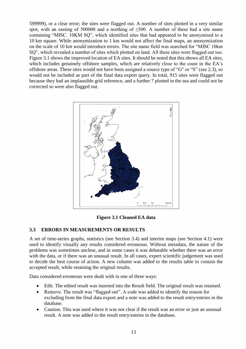
Figure 3.1 shows the improved location of EA sites. It should be noted that this shows all EA sites,

which includes genuinely offshore samples, which are relatively close to the coast in the EA’s

offshore areas. These sites would not have been assigned a source type of “G” or “S” (see 2.3), so

would not be included as part of the final data export query. In total, 915 sites were flagged out

because they had an implausible grid reference, and a further 7 plotted in the sea and could not be

corrected so were also flagged out.

Figure 3.1 Cleaned EA data

3.3 ERRORS IN MEASUREMENTS OR RESULTS

A set of time-series graphs, statistics (see Section 3.4) and interim maps (see Section 4.1) were

used to identify visually any results considered erroneous. Without metadata, the nature of the

problems was sometimes unclear, and in some cases it was debatable whether there was an error

with the data, or if there was an unusual result. In all cases, expert scientific judgement was used

to decide the best course of action. A new column was added to the results table to contain the

accepted result, while retaining the original results.

Data considered erroneous were dealt with in one of three ways:

Edit. The edited result was inserted into the Result field. The original result was retained.

Remove. The result was “flagged out”. A code was added to identify the reason for

excluding from the final data export and a note was added to the result entry/entries in the

database.

Caution. This was used where it was not clear if the result was an error or just an unusual

result. A note was added to the result entry/entries in the database.

14

3.3.1 Incorrect units

A number of results within the PUB database displayed unrealistically high values, these were

evident in the time-series plots. For example, some F data for distinct periods had parameter

concentrations far in excess of the PCV. Some of these were elevated 1000 times larger than the

rest of the data. It is likely that these represent data reported in incorrect units. The DWI confirmed

this was a likely conclusion given that some parameters’ reporting units were changed in 2000,

and may represent an error relating to this. Boron and Cu were both also subject to changes of

reporting units and selected data displayed the same problem. All the data for Thames Water for

example, were elevated relative to other water companies’ data and the PCV, indicating all data

were reported incorrectly. In total, 143 F results, 191 B results, and 9,179 Cu results were edited

in order to convert into the correct units.

When the problem was initially identified, it had been thought that an algorithm could be produced

based on data distribution to provide an indication of a value above which the data were incorrect.

However, there was no simple way to edit all such data for a given parameter without inadvertently

changing correct data. Instead the data for each water company were examined individually, and

queried according to date ranges and relevant ranges of values. Queries could then be written to

ensure that only the required data were changed.

3.3.2 Misrecorded pH

The pH scale is typically presented as being 0–14. However the scale is open-ended (Lim, 2006).

Values of pH <1 and >14 are possible and have been prepared in chemical laboratories (Nordstrom

et al., 2000). It is difficult to measure pH values which occur beyond 0–14 (Lim, 2006), and a

specific set of conditions are needed for such values to exist in the natural environment. Values of

pH as low as -3.6 have been measured in mine waters from Iron Mountain, California (Nordstrom

et al., 2000). It is, however unlikely that natural waters in the UK would have pH values beyond

the range of 0–14, and with this in mind, where values exceeded pH 14 they were edited or flagged

out. By the nature of pH measurement, the values would have been typed into databases manually,

and this would make typographical errors a possibility. It did mean that every value deemed

incorrect had to be identified and dealt with individually, but sometimes the true result was clear

when compared to the other values recorded at the same site. For example, at one site the 1363 pH

measurements ranged from 6.68 to 8.38, with one value of 726. This was corrected to 7.26. Where

the pH value was obviously incorrect, but it was not clear what the result should be, it was flagged

out. When the pH value was unlikely, given the range of other values at the same site, a caution

note was added. In total, 162 pH values were changed, removed, or a cautioned.

3.3.3 Elevated concentrations

In some instances results had elevated concentrations that were either not part of a separate

population to the majority of the data, or were slightly elevated above the rest of the data. Affected

data were all old (pre-2011), and thus of lower importance to the geostatistical modelling process.

These results were flagged out as the correct result was unclear.

The NO3 data reported by Welsh Water (DWR) after 10/12/2012 were mostly reported as censored.

The likely real detection limit was selected, as the lowest value which occurred many times, and

the remainder had the “<” removed from the qualifier field. Caution should be taken with these

data, as any higher detection limits used (as a result of sample dilutions, or changes in reported

detection limit) now would not be recognised.

3.3.4 Outliers

Most environmental data will have outliers. However, some were so large that they would skew

the meaningful data. In these cases, a judgement was made to flag out the result. Where an outlier

was more marginal, a cautionary note was added.

15

3.3.5 Implausible results

In some cases unusual results warranted further investigation. A group of results with high

concentrations of Pb (up to 54700 µg/L) was identified, within the NRWr data. The highest of

these were all from the same site. As these appeared to be a normal population, rather than outliers,

the location was identified to establish whether such concentrations could be considered

reasonable. The grid reference plotted on a government building, which would be a reason to flag

out such a result (as occurred with the PRI data, see Section 3.1.2). However this building is on a

former oil refinery site, which is undergoing remediation, and it is possible that the grid reference

had been anonymised, or the stream diverted. With this in mind, a cautionary note was applied to

all the results from this site. The next highest Pb values in the NRWr database (up to 6170 µg/L)

were from multiple sites which all plotted on an abandoned Pb-Zn mine site. These were therefore

reasonable results and no notes were applied.

3.3.6 Negative values and zeros

While not an example of incorrect data, where the data were raw it was possible for small

negative values to exist in the results field, and where data had been processed there were some

values set to zero. Neither of these are ideal from a statistical or mapping viewpoint. However,

zeros are easier to take account of, and so any negative values were changed to be 0 in the results

field.

3.3.7 Spatial anomalies

Once the time-series graphs and statistics had been used to remove numerous errors a set of

preliminary maps (Section 4) created from the data, was examined. These maps highlighted the

outstanding units problems discussed above.

3.4 EXPLORATORY DATA ANALYSIS

3.4.1 Summary statistic calculations

Regression on Order Statistics (ROS) was used to calculate the median and mean values taking

into account the non-detect data. The method assumes the data follow a lognormal distribution. It

performs a regression on the data assuming lognormal quantiles. The line created predicts

unknown observations. Summary statistics can be computed based on the predicted observations

and on the non-censored observations. The idea behind ROS is that if the data follow a lognormal

distribution (or some other known distribution), then a probability plot of the log of the ordered

data versus the quantiles of a standardised normal should give a straight line. Thus, the mean and

standard deviation for the log of the data can be obtained. The mean is estimated using the intercept

and the standard deviation using the slope of the line. Subsequently, unknown values below the

censoring limit can be extrapolated (using the estimated parameters). Observations for all potential

values are known, and all the summary statistics can be estimated. Transformation bias is a concern

any time the log of data is used. To help correct this, quantities from a normal distribution are first

transformed to lognormal quantities. The summary statistics are then computed on the scale of the

original data (Lee and Helsel, 2005b, Lee and Helsel, 2005a) ROS is implemented in R in the

NADA package:

almost any sample size is sufficient for ROS. Sample size does not need to be greater

than 30;

ROS works for small datasets, as well as large ones;

censoring percentages up to 80% can be tolerated although results should be interpreted

carefully in this situation;

this method is resistant to non-normality in the data. Even in the presence of skewed

datasets, meaningful inference can be achieved.

16

TREND DETECTION

Two methods were used to look for trends in the data.

The non-parametric Cox and Stuart trend test (as implemented in the “trend” R package) was used

where the series is divided into three. The data of the first third of the series are compared to see

if they are larger or smaller than the data of the last third of the series. A test statistic of the Cox-

Stuart trend test for n > 30 was calculated and this was used to decide if there is a significant

difference and hence whether there is a significant trend.

A robust linear regression (as implemented in the “mblm” R package) of the time-ordered data

was carried out producing the slope of the regression and its 95th percentile uncertainty limits. If

both the upper and lower limits are positive, this suggests a positive trend; if one is negative and

one is positive, this suggests the slope is not significantly different from 0; and if both limits are

negative, this suggests a negative trend.

3.4.2 Presentation of statistical analysis

Summary statistical data and trend analyses were compiled into summary tables using R. The data

were kept separate according to the water type (groundwater or surface water) and their source

database, with the exception of EA, NRWo, and NRWr, which were combined, and given the code

CMB to denote these were combined data. Statistics were summarised according to categories

relevant to each dataset. For example the PUB data are divided according to water company, local

authority code, and surface geology type. Summary tables can be used to obtain information to

supplement the final risk maps and are available from DWI on request.

Time-series graphs were produced using the ggplot2 package (Wickham, 2016) in R for the CMB

and PUB data. These were the largest datasets and could be split into a relatively small number of

categories (EA area and water company, respectively) for further examination. While these did not

provide much meaningful information on trend analysis, they could be used for data quality

investigation. The remaining databases either did not contain time-series data (GB), have an

insufficient volume of data (CEH) or had too many categories (PRI – split into local authority

areas) to provide any insight into the data quality. The produced graphs were used to identify

numerous data-quality issues (See Section 3.3).

The trend detection data were used to produce a series of maps using a combination of the

“ggplot2” (Wickham, 2016) and the “sf” spatial packages (Pebesma, 2018) in R. These are not

reported here but were used to assist with the recommendations of the project (Section 6).

17

4 Water-quality mapping

4.1 PROBABILISTIC MAPPING OF THE WATER-QUALITY PARAMETERS

4.1.1 Overview

In line with the requirements of EC Directive 2015/1787 for assessing drinking-water monitoring

data, analyses selected for mapping were restricted to the last three years’ worth for each data

source. Based on the water-quality measurements since 2015, maps were produced of the expected

value of an additional measurement of each parameter. These predictions are uncertain to a degree

that varies in space and for different parameters. Therefore, maps of the 95th percentile for an

additional measurement were also produced for each parameter. The 95th percentile is the value of

the parameter for which there is a five percent (or 1 in 20) chance that it is exceeded. These maps

consisted of predictions at the nodes of a grid with 1 km spacing, covering the whole of England

and Wales.

There were a number of challenges associated with using the water-quality dataset gathered in this

project for this purpose. The locations and times of each measurement within the dataset were not

chosen according to an unbiased statistical design and were therefore not necessarily completely

representative of the values that might be expected across England and Wales. For example, there

could be spatial clustering of measurements if a portion of the data had been taken from a research

project that included intensive observation of a particular aquifer, river or catchment.

Alternatively, additional observations might have been made to monitor parameters intensively in

regions or at times where they are known to be close to the PCV, leading to a disproportionate

number of large values in the dataset. Some of the measurements could and would have been made

to monitor water-quality status on sites of known local contamination (e.g. mines, oil refineries).

Although all efforts were made to restrict water-quality data to those likely to be representative for

the location, since the reasons for making a measurement at a particular location and time are not

always recorded, it is not in all cases possible to make adjustments for preferential sampling. In

addition, there might be large regions where measurements of particular parameters are absent or

sparse and it is therefore not possible to predict precisely their statistical distribution for that

region.

Measurements of some of the parameters are highly variable in both time and space. This variation

can mask the underlying pattern of variation of the measurements.

The geostatistical methodologies (Bardossy, 2002, Marchant, 2018, Webster and Oliver, 2007)

used in this project rely on the measurements of a particular parameter being spatially correlated

(i.e. measurements made close together are likely to be more similar than those made a long

distance apart). If this is the case, it is possible to use measurements from neighbouring locations

to make predictions of the parameter where it has not been measured. The degree of spatial

correlation is quantified within the geostatistical methodology. If no spatial correlation is apparent

then the variation of the parameter has no discernible spatial pattern and the predictions of a

parameter will be identical across the study region. For example, in a study of the concentrations

of persistent organic pollutants in the soils of northern France, Villanneau et al. (2011) found that

22 of the 31 pollutants under investigation could not be mapped for this reason.

The patterns of variation can be too complex to be estimated adequately by a tractable statistical

model.

For some parameters, a substantial proportion of the measurements fall below the detection limit

of the laboratory procedures. This means that the measurement only indicates an upper limit for

the value of the parameter at the relevant location and time. Depending on how these

measurements are treated in the statistical analysis, there is a potential for them to lead to biased

predictions of the parameter. If, for example, the detection limit is close to or beyond 30% of the

18

PCV, there might be little relevant information to determine the probability that this threshold is

exceeded. Also, the detection limits can and do vary in space and time which can produce

misleading spatial and temporal trends in the recorded values.

Previous sections of this report have described how many erroneous measurements were identified

and removed from the dataset because, for example, the recorded values were implausible or

inconsistent with the rest of the dataset, there were large systematic differences between recorded

values from different sources, or the recorded locations did not fall within England or Wales.

However, given the large variability of some parameters it would not have been possible to identify

more subtle errors such as a measurement being allocated to the wrong location within England

and Wales or less obvious mistakes in recording the measured value. Some large recorded values

of parameters might appear unlikely but are not removed from the dataset since they might indicate

an anomaly that this monitoring should identify.

The final challenge results from the size of the dataset. For some parameters, many thousands of

measurements have been made since 2015 and this limits the computational methods that can be

applied. If the focus of the study was on the underlying variation in the parameter values then it

might be acceptable to subsample such measurements. However, this would risk the removal of

the large values, which are of particular interest in studies of water contamination.

4.1.2 The statistical model

This section describes the technical details of the statistical approach adopted. With the exception

of the strategies for accounting for non-detect observations, the approach and Matlab software

have previously been used to map soil inorganic carbon concentrations across France (Marchant

et al., 2015). Further details of the approach are provided in Marchant (2018). In the following

section, the approach is demonstrated for the measurements of some water-quality parameters

compiled for this project.

The mapping methodology is required to predict the entire statistical distribution of each parameter

at each prediction location so that both the expected value and corresponding uncertainty for the

parameter can be determined. This necessitates the use of a statistical model to represent the

variation of the data rather than an interpolation technique such as inverse-distance weighting

which would only predict the expected value of the parameter (Webster and Oliver, 2007). The

model must be able to handle there being multiple measurements made at the same location. In

statistical notation the model takes the form:

𝑧(𝐱, 𝑡) = µ + 𝑢(𝐱) + 𝜀.

Here, 𝑧(𝐱, 𝑡) denotes the measured value of the transformed (see below) parameter at location 𝐱

and time 𝑡, µ is the expected value of the transformed parameter across the study region, the 𝑢(𝐱)

term accounts for the spatial variation of the transformed parameter and the 𝜀 accounts for the

variation in transformed measurements from the same location made at different times.

A number of standard assumptions (Webster and Oliver, 2007) are made to simplify the model.

The 𝑢(𝐱) term is assumed to be Gaussian, second order stationary and spatially correlated. This

means that the values of 𝑢(𝐱) are drawn from a Gaussian (i.e. Normal) distribution and the same

degree of spatial correlation occurs across the study region. The 𝜀 term is assumed to be Gaussian

and independent (i.e. not spatially or temporally correlated) and each location has the same degree

of temporal variability.

Many water-quality parameters have a highly skewed distribution (i.e. the histograms of measured

values are non-symmetric because of a small proportion of large values) which is not consistent

with the Gaussian assumptions in the above model. Therefore, prior to modelling they were

transformed to a Gaussian variable with mean zero and a standard deviation of one by a non-

parametric method. If there are 𝑛 observations of a parameter this non-parametric transformation

19

requires a length 𝑛 Gaussian variable with mean zero and variance one. These 𝑛 values are the

values of the transformed variable. The location and time with the largest observed parameter

value is allocated the largest transformed value, the location and time with the second largest

observed parameter value is allocated the second largest transformed value and so on. The values

of the regulatory thresholds can also be transformed to be consistent with this transformed variable.

In addition to ensuring that the data are more consistent with the statistical model this

transformation makes the model more robust to extreme or outlying values. Without the

transformation, a single extreme value could have a large effect on the overall mean of the data.

With the transformed variable, this effect is moderated because it can only take values consistent

with a zero-mean Gaussian distribution of unit variance.

The 𝑢(𝐱) term controls the spatial variation in the model and the degree of spatial correlation

between 𝑢(𝐱) values from adjacent locations controls the degree of spatial pattern in the maps that

will eventually result. This degree of spatial correlation must be estimated from the transformed

data. In the geostatistics literature (Webster and Oliver, 2007), spatial correlation is often

expressed by a variogram. This is a model of the semi-variance (i.e. half of the expected squared

difference between a pair of values of 𝑢(𝐱)) and the distance that separates them. The exponential

variogram functions used in this study do not decrease as this separation or lag distance increases.

If there is strong spatial correlation then the semi-variance will remain below one (the variance of

the transformed variable) for substantial lag distances and a strong spatial pattern will be apparent

in predicted maps of the transformed variable. If there is no spatial correlation then the semi-

variance will take a constant value close to one for all lag distances and all of the predicted values

of the transformed variable will have the same value.

The variogram is commonly estimated by an approach called the method of moments which

involves allocating pairs of observations to ‘lag bins’ according to the lag distance between them

and then calculating the average semi-variance for each lag bin. This approach has been shown to

be biased for data that are strongly clustered in space (Marchant et al., 2013). We therefore use the

more computationally demanding but unbiased residual maximum likelihood estimator (REML;

Lark et al., 2006). The variogram of the 𝑢(𝐱) term in the model reflects the degree of spatial

correlation of the temporal average of the water-quality measurements at each location. If the

variance of the 𝜀 term is added, then the resultant variogram reflects both the spatial variation of

the site averages and the temporal variation of measurements from the same site.

Once the variogram and other parameters of the model have been estimated by REML, they can

be used to predict the transformed parameter on the nodes of the 1 km grid covering England and

Wales. This process, often referred to as kriging (Webster and Oliver, 2007), leads to maps of the

expected value of the transformed parameter and the standard error of these predictions. The

assumptions of the statistical model imply that at each location the predicted distribution is

Gaussian. Therefore, the mean and standard error are sufficient information to determine the

probability that a randomly drawn measurement of the transformed parameter exceeds any of the

transformed PCVs. The expected value of the transformed parameter and its standard error can be

back-transformed to the original units of the water-quality parameter to produce maps of the

expected value and any specified percentile.

There remains the issue of how to handle observations of the water-quality parameter that are

below the detection limit. Bardossy (2002) suggests a number of strategies. All values below

detection limit could be treated as zero but this will negatively bias (i.e. erroneously decrease) the

predicted values. Alternatively, they could all be treated as if they were equal to the detection limit,

which would positively bias the predictions. These and any other strategies that replace the non-

detects with a constant will also increase the degree of spatial correlation within the estimated

variogram since the replaced observations will be identical and therefore suggest strong correlation

between measurements from the corresponding locations. Bardossy (2002) opted for an indicator

approach to map the probabilities of regulatory thresholds for groundwater parameters being

exceeded across a region of Germany. In this approach the measured data are replaced by an

20

indicator variable which is one if the measurement is greater than a regulatory threshold (such as

the PCV) and zero otherwise. If the detection limit is less than the threshold, the exact value of

non-detects is not required. If spatial prediction is applied to this indicator variable, a prediction

of the probability of exceedance results. Bardossy (2002) demonstrated how this can lead to

realistic exceedance threshold maps when the observations are dispersed across the study region.

However, it does discard information about the variation of the parameter since a measurement

that is marginally below the threshold is treated identically to one that is below the detection limit.

Also, where spatially isolated exceedances of the PCV occur, this leads to unrealistic circular

patterns in the exceedance maps.

Table 4. Summary of water-quality measurements since January 2015

N n

(prop)

sites sites

(prop)

PCV Prop

>PCV

DL Prop

<DL

Groundwater

Al 21405 0.16 5522 0.48 200 0.02 10 0.81

As 14214 0.22 3440 0.54 10 0.09 1 0.66

B 11981 0.15 2566 0.40 1 0.01 0.1 0.89

CN 8715 0.22 2068 0.54 50 0.00 5 0.99

Cd 13565 0.15 2988 0.41 5 0.00 0.25 0.97

Cl 29278 0.19 3808 0.48 250 0.01 10 0.04

Col 17343 0.19 5161 0.61 20 0.01 1 0.76

Conductivity 49828 0.17 9063 0.52 2500 0.00 0.06 0.00

Cr 14134 0.17 2986 0.42 50 0.00 1 0.95

Cu 13989 0.16 4006 0.41 2 0.00 0.1 0.93

F 20536 0.21 3613 0.50 1.5 0.02 0.05 0.12

Fe 39902 0.17 7065 0.50 200 0.19 30 0.66

Gross α 2529 0.42 415 0.79 0.1 0.14 0.03 0.45

Gross β 2370 0.42 431 0.83 1 0.00 0.28 0.96

Hg 8697 0.20 2099 0.51 1 0.00 0.1 0.99

Mn 43134 0.17 7964 0.50 50 0.13 10 0.73

NH4 46843 0.19 7830 0.56 0.5 0.04 0.04 0.81

NO2 32639 0.20 5018 0.60 0.5 0.00 0.01 0.91

NO3 48521 0.17 7069 0.53 50 0.13 4 0.19

Na 16454 0.16 2978 0.42 200 0.01 2 0.00

Ni 15673 0.16 3119 0.42 20 0.02 2 0.72

Pb 16588 0.17 4704 0.44 10 0.02 2 0.91

Sb 9116 0.13 2075 0.34 5 0.00 1 0.99

Se 11066 0.20 2483 0.53 10 0.00 1 0.77

TOC 11494 0.23 1438 0.38 NaN 0.00 0.5 0.28

Turbidity 47115 0.15 7271 0.57 4 0.07 0.25 0.72

pH 48544 0.15 9150 0.52 9.5 0.06 0 0.00

Surface water

Al 16178 0.15 1010 0.38 200 0.21 10 0.05

As 6932 0.09 445 0.23 10 0.05 1 0.53

B 6331 0.09 538 0.26 1 0.00 0.1 0.92

CN 13126 0.06 1160 0.19 50 0.00 0.01 0.92

Cd 14611 0.08 1288 0.21 5 0.02 5 0.98

Cl 24615 0.04 1965 0.05 250 0.03 5 0.03

Col 19075 0.13 1071 0.44 20 0.40 5 0.10

21

Conductivity

y

19075 0.13 1071 0.44 2500 0.00 5 0.10

Cr 13620 0.08 1368 0.25 50 0.00 1 0.88

Cu 13250 0.06 1163 0.19 2 0.00 0.1 0.98

F 6168 0.06 399 0.01 1.5 0.00 0.05 0.19

Fe 18765 0.09 1150 0.28 200 0.61 30 0.09

Gross α 410 0.43 65 0.86 0.1 0.01 0.03 0.83

Gross β 411 0.44 66 0.89 1 0.01 0.28 0.97

Hg 7923 0.08 556 0.24 1 0.00 0.1 0.99

Mn 38247 0.17 2733 0.56 50 0.28 10 0.25

NH4 12263

5

0.09 8736 0.45 0.5 0.05 0.04 0.51

NO2 23222 0.15 1453 0.15 0.5 0.00 0.01 0.52

NO3 12507

8

0.10 8213 0.19 50 0.07 4 0.22

Na 10280 0.13 686 0.29 200 0.01 2 0.00

Ni 12742 0.08 1068 0.20 20 0.02 2 0.55

Pb 14745 0.09 1239 0.23 10 0.11 2 0.71

Sb 2822 0.24 196 0.44 5 0.00 1 0.99

Se 4486 0.11 253 0.23 10 0.00 1 0.96

TOC 9951 0.11 350 0.13 NaN 0.00 0.5 0.01

Turbidity 21394 0.07 1436 0.30 4 0.40 1 0.18

pH 14131

6

0.10 9187 0.16 9.5 0.02 0 0.00

PCV units as for Table 1. n: number of measurements; n (prop): proportion of measurements in entire database made

since Jan 2015; n site: number of distinct sites from which measurements are obtained; sites (prop): proportion of sites

in entire database where measurement has been made since Jan 2015; prop>PCV: proportion of measurements greater

than PCV (or outwith the PCV range for pH); DL: detection limit; prop<DL: proportion of measurements less than

detection limit;. NaN: not a number.

We therefore replace each non-detect value with a random value between zero and the detection

limit. This reflects our level of knowledge about these variables and will not lead to exaggeration

of the degree of spatial correlation exhibited by the data. The approach will lead to differences in

the predictions each time the algorithm is run. Therefore, the algorithm was re-run 100 times, re-

selecting the random non-detect values each time, and the average predictions and 95th percentiles

were quoted in our outputs. The recorded detection limits for each parameter vary in time and

according to the organisation providing the data. This might reflect differences in the laboratory

protocols and equipment used by different organisations or changes to these protocols over time.

We use a single detection limit for each parameter to avoid its variation leading to spurious spatial

trends. The detection limits quoted by the Environment Agency tend to be more stable than those

from other organisations. Therefore, for parameters where there are more than 10 examples of

detection limit values within the Environment Agency data, the mode of these 10 values was

initially considered to be the detection limit. If there are fewer than 10 non-detect measurements

amongst the Environment Agency data then the detection limit was initially considered to be equal

to the mode of the detection-limit values from all sources. These initial detection limits were then

reviewed and adjustments made where appropriate. Any recorded measurements below this

detection limit are treated as non-detects. Any measurement larger than this detection limit but

marked as being at detection limit were omitted from the analysis.

4.1.3 Demonstration of the probabilistic mapping methodology

In this section the mapping methodology is primarily presented with reference to total groundwater

aluminium concentrations. Contrasting results for other water-quality parameters are also shown.

Figure 4.1 (left) shows a histogram of the 21,405 measurements of groundwater aluminium

concentrations recorded since the start of 2015. Only 19% of the recorded measurements are

greater than the detection limit of 10 µg/L. The distribution is very positively skewed with only

22

2% of measurements exceeding the PCV of 200 µg/L but the largest measurement being

15,900 µg/L. The skewness is so pronounced that the vast majority of the observations are

contained in the first two of the 100 bins of the histogram. Webster and Oliver (2007) suggest that

a variable with absolute skewness less than one might be considered to be approximately Gaussian

whereas the skewness of this population is 31.3. This emphasises the need to transform the

groundwater aluminium concentrations before representing them by a model which assumes they

result from a Gaussian distribution. The non-parametric transformation described in the previous

section leads to an exact Gaussian histogram (Figure 4.1, right). The 30%, 60% and 100% PCV

threshold values for the transformed variable are shown in this plot and all are substantially larger

than the detection limit of approximately 0.74.

Figure 4.1 Histograms of observed total groundwater aluminium concentrations in µg/L

(left) and transformed units (right). Vertical black lines indicate 30%, 60% and 100% of the

PCV. Vertical red line indicates the modal Environment Agency detection limit within the

dataset

The most recent transformed aluminium measurement from each of the 5522 sites at which it is

measured is shown in Figure 4.2 (left). There is reasonable spatial coverage of England and Wales

and there is some evidence of a fairly small degree of spatial correlation with some patches of

consistently large values (e.g. in central Wales) and consistently small values (e.g. within the Chalk

aquifer in southern England). There are no obvious large-scale spatial trends in the data. The

variogram of the 𝑢(𝐱) term in our statistical model is shown in red in Figure 4.2 (right). Again,

some spatial correlation is apparent with temporal average measurements from sites separated by

a very short distance apart having a semi-variance (half of the expected squared difference between

temporal averages) of around 0.2 whereas this increases to 0.37 for sites separated by 50 km. The

within-site (i.e. temporal) variation of measurements is larger than that explained by the 𝑢(𝐱) term

and when this variation is added to the 𝑢(𝐱) variogram to produce the black line in Figure 4.2

(right), it is apparent that more than 80% of the variation is spatially unstructured.

23

Figure 4.2 Most recent observation of total groundwater aluminium at each site in

normalised units (left) and variograms of the temporal average of the normalised

groundwater aluminium observations (in red, right)

This is sufficient spatial correlation to lead to some pattern in the predicted map of the normalised

total groundwater aluminium distribution (Figure 4.3, left) although the standard error of this

prediction (Figure 4.3, right) is close to 1 everywhere. The large standard errors reflect the large

degree of temporal variation in the measurements from each site. Standard errors are slightly larger

in regions where there are few or no observations. We explore the uncertainty of the spatial pattern

in the predicted maps by calculating the expected concordance correlation between the predicted

and actual temporal average concentration at each site using a formula derived in Lark (2015). The

concordance correlation is a measure of the degree to which the predicted and actual values are

expected to be equal. A concordance correlation of one indicates that they are expected to be

exactly equal whereas a concordance correlation of zero indicates that they are unrelated. Figure

4.4 shows that for locations where there are a substantial number of nearby measurements there is

reasonable concordance correlation between predicted and actual temporal averages of above 0.6.

The correlation is greater than 0.4 for 50% of the locations in England and Wales. Where there are

few or no data the concordance correlation is close to zero.

The predicted total groundwater aluminium concentration in µg/L is shown in Figure 4.5 (left) and

the 95th percentile is shown in Figure 4.5 (right). There are some regions which are distant from

any observations (e.g. the extreme south-west of Pembrokeshire and Dungeness Peninsula of south

Kent). In these regions the predicted distribution of the groundwater aluminium concentration

tends toward the observed distribution of the entire dataset. These predictions are not informed by

any local measurements. These are the sites with very small correlation in Figure 4.4. The 95th

percentile values at these sites are much larger than the expected value reflecting the uncertainty

in these predictions (Figure 4.3). At sites with more nearby data and lower uncertainty the expected

and 95th percentile values are more similar to each other.

24

Figure 4.3 Predictions of total groundwater aluminium concentration in normalised units

(left) and standard error of these predictions (right)

Figure 4.4 Expected concordance correlation between predicted temporal average

groundwater aluminium concentration in normalised units and actual value in normalised

units

Figure 4.5 Predictions of expected total groundwater aluminium concentration in µg/L (left)

and predicted 95th percentile (right). Colour scales are censored at PCV value of 200 µg/L

so that darkest red indicates prediction greater than or equal to 200 µg/L

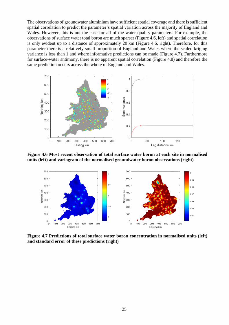
25

The observations of groundwater aluminium have sufficient spatial coverage and there is sufficient

spatial correlation to predict the parameter’s spatial variation across the majority of England and

Wales. However, this is not the case for all of the water-quality parameters. For example, the

observations of surface water total boron are much sparser (Figure 4.6, left) and spatial correlation

is only evident up to a distance of approximately 20 km (Figure 4.6, right). Therefore, for this

parameter there is a relatively small proportion of England and Wales where the scaled kriging

variance is less than 1 and where informative predictions can be made (Figure 4.7). Furthermore

for surface-water antimony, there is no apparent spatial correlation (Figure 4.8) and therefore the

same prediction occurs across the whole of England and Wales.

Figure 4.6 Most recent observation of total surface water boron at each site in normalised

units (left) and variogram of the normalised groundwater boron observations (right)

Figure 4.7 Predictions of total surface water boron concentration in normalised units (left)

and standard error of these predictions (right)

26

Figure 4.8 Most recent observation of total surface water antimony at each site in normalised

units (left) and variogram of the normalised observations (right)

In the case of pH, the PCV is given as a range (6.5–9.5) rather than a single value. Observations

beyond the PCV could therefore be lower as well as higher. For this reason, for pH only,

distributions of the 5th percentile as well as the 95th percentile were computed to indicate plausible

values at each end of the range. The 5th percentile would be the value of pH for which there is a

five percent (1 in 20) chance that it is lower than the minimum PCV.

4.1.4 Interpretation of mapped outputs

Two mapped outputs are presented for each parameter. These are the expected value and 95th

percentile value. An example of these outputs is shown for aluminium in Figure 4.5 (see also

Appendix 1). We assume that users of the outputs will be interested in comparing these values to

the PCV or thresholds that are fractions of the PCV. Therefore, we truncate the colour scale of the

maps to run between zero and the PCV (note, the colour ramp differs slightly from that in the

accompanying GIS).

Both of these outputs consider a potential measurement of the water-quality parameter made at a

new borehole situated at the centre of each 1-km grid square in England and Wales. The statistical

model described in the previous section can be used to predict the value of the measurement and

this prediction is subject to uncertainty. The model will predict that a range of values of the

measurement are possible and will assign different probabilities of occurrence to each value. The

expected value is calculated by multiplying each of the possible values by its probability and then

summing all of those values.

The expected value can be interpreted as the anticipated value of the measurement.

The model predicts that there is a 0.05 or 1-in-20 probability that the measurement will exceed the

95th percentile. The difference between the expected and 95th percentile values is indicative of the

amount of uncertainty in the prediction. If there were no uncertainty, then these values would be

equal. If there were considerable uncertainty, then the 95th percentile value would be much greater

than the expected value.

The 95th percentile can be interpreted as a plausible but larger than anticipated value for the

measurement. The model predicts that there is a 0.05 or 1-in-20 probability that the measurement

exceeds the 95th percentile. For pH, the 5th percentile can be interpreted as a plausible but lower

than anticipated value.

27

Exemplar mapped outputs for groundwater and surface-water nickel are illustrated in Figure 4.9,

Figure 4.10, Figure 4.11 and Figure 4.12. Figure 4.9 shows the measurement locations and

concordance correlation for groundwater nickel. The measurements are mostly made on major

aquifers. In the vicinity of measurements, there is a large concordance correlation but upon moving

away from these locations, the concordance correlation decreases quickly. This is indicative of

measurements only being spatially correlated when they are separated by short distances.

Locations which are not close to a measurement have an expected concentration (Figure 4.10, left)

of around 2 µg/L. This is approximately the average value of all the measured values and is

considerably less than the PCV of 20 µg/L. There is more variation in the expected value close to

measurement points with some small regions exceeding the PCV, whereas others have values less

than 2 µg/L. The 95th percentile values (Figure 4.10, right) are larger than the expected values. At

locations that are not close to any measurements, they have increased by around 8 µg/L because

these predictions are uncertain. Close to measurements, the increase is often smaller and some

locations have a 95th percentile value less than 2 µg/L. At these locations the nearby measurements

mean that the concentration can be predicted with much more certainty.

Figure 4.9 Locations of measurements of groundwater nickel since 2015 (left) and expected

concordance correlation between predicted temporal average groundwater nickel

concentration in normalised units and actual value in normalised units (right)

Figure 4.10 Predictions of expected groundwater nickel concentration in µg/L (left) and 95th

percentile (right). Colour scales are censored at PCV of 20 µg/L so that darkest red indicates

prediction equal to or greater than 20 µg/L

The concordance correlation for surface-water nickel also decreases upon moving away from

measurement locations but the rate of decrease is slower (Figure 4.11). Measurements of surface-

water nickel concentration are spatially correlated over larger distances. The map of expected

surface-water nickel values (Figure 4.12, left) is smoother than its groundwater counterpart and it

has larger regions which exceed the PCV. Again, the difference between the 95th percentile and

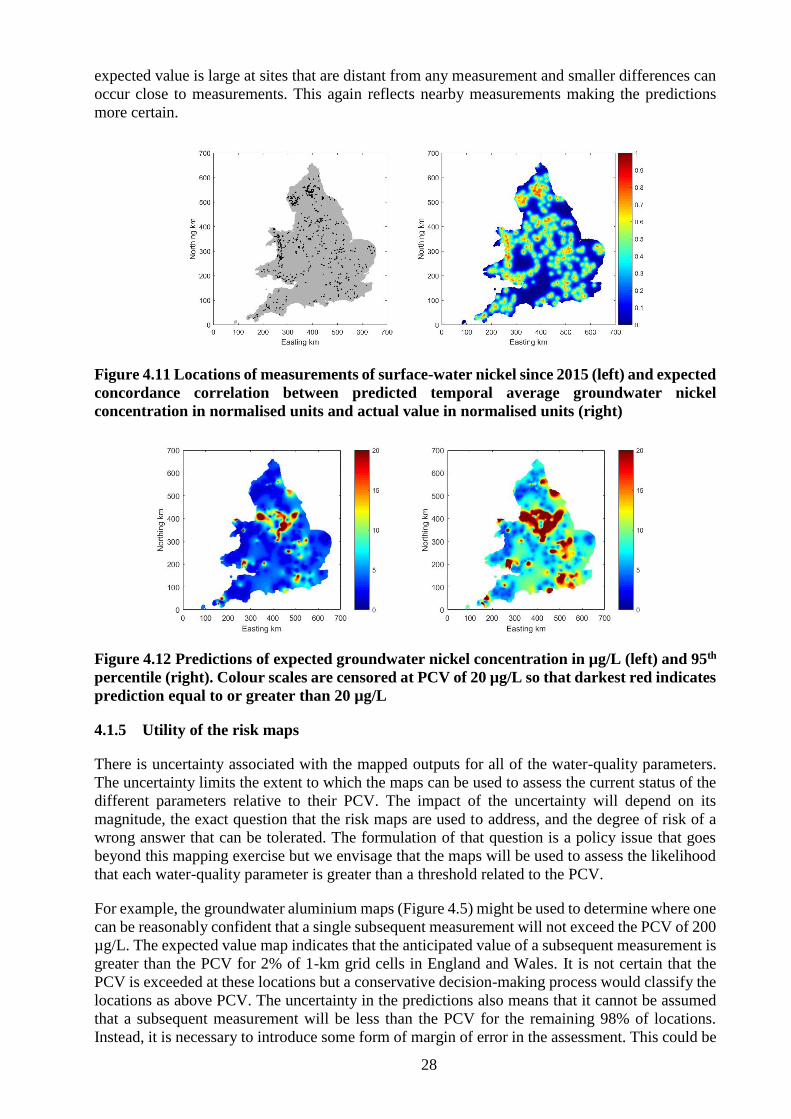
28

expected value is large at sites that are distant from any measurement and smaller differences can

occur close to measurements. This again reflects nearby measurements making the predictions

more certain.

Figure 4.11 Locations of measurements of surface-water nickel since 2015 (left) and expected

concordance correlation between predicted temporal average groundwater nickel

concentration in normalised units and actual value in normalised units (right)

Figure 4.12 Predictions of expected groundwater nickel concentration in µg/L (left) and 95th

percentile (right). Colour scales are censored at PCV of 20 µg/L so that darkest red indicates

prediction equal to or greater than 20 µg/L

4.1.5 Utility of the risk maps

There is uncertainty associated with the mapped outputs for all of the water-quality parameters.

The uncertainty limits the extent to which the maps can be used to assess the current status of the

different parameters relative to their PCV. The impact of the uncertainty will depend on its

magnitude, the exact question that the risk maps are used to address, and the degree of risk of a

wrong answer that can be tolerated. The formulation of that question is a policy issue that goes

beyond this mapping exercise but we envisage that the maps will be used to assess the likelihood

that each water-quality parameter is greater than a threshold related to the PCV.

For example, the groundwater aluminium maps (Figure 4.5) might be used to determine where one

can be reasonably confident that a single subsequent measurement will not exceed the PCV of 200

µg/L. The expected value map indicates that the anticipated value of a subsequent measurement is

greater than the PCV for 2% of 1-km grid cells in England and Wales. It is not certain that the

PCV is exceeded at these locations but a conservative decision-making process would classify the

locations as above PCV. The uncertainty in the predictions also means that it cannot be assumed

that a subsequent measurement will be less than the PCV for the remaining 98% of locations.

Instead, it is necessary to introduce some form of margin of error in the assessment. This could be

29

achieved by considering the 95th percentile for the remaining 98% of sites. If the 95th percentile is

less than the PCV for a location then the model is indicating that there is less than a 1-in-20 chance

that the subsequent measurement at the location will exceed the PCV. For groundwater aluminium,

this is the case for 77% of the locations. This leaves 21% of locations where the anticipated value

is less than the PCV but the 95th percentile is greater than the PCV. At these sites, although a

greater than PCV subsequent measurement is not expected, there is a more than 1-in-20 chance of

it occurring. For these sites, the uncertainty in the predictions is preventing a judgement about

whether the PCV is likely to be exceeded. The proportion of sites where a decision about water-

quality status can be made by these criteria (i.e. in the case of groundwater aluminium

0.02+0.77=0.79) could be considered a measure of the utility of the maps. This proportion will

vary both with the magnitude of the uncertainty and the closeness of the model predictions to the

threshold. For example, the maps for a particular parameter might have no spatial pattern and be

highly uncertain but if the considered threshold is sufficiently large to be always greater than the

95th percentile then a decision is possible by these criteria at all sites. One circumstance where this

situation can arise is where almost all measurements are less than the detection limit. Then it is

very challenging to establish any spatial pattern to the measurements but the measured values are

sufficiently small to indicate that exceedance of the PCV is unlikely.

Table 5 shows the proportion of sites where a decision is possible by these criteria for all of the

parameters where the thresholds are the PCV, 60% of the PCV and 30% of the PCV. For pH, there

is an upper and lower PCV (9.5 and 6.5) and the only decision considered is whether the

subsequent measurement is likely to be within this range. When the threshold is the value of the

PCV, a decision is possible for an average proportion of 0.84 of England and Wales. For this

threshold, there are six parameters for which a decision is possible for less than half of England

and Wales. These are groundwater total gross alpha, groundwater manganese, groundwater nitrate,

groundwater turbidity, surface-water aluminium and surface-water manganese.

Some caution should be applied when using the mapped outputs. The uncertainty quantified by

the statistical model is primarily the result of sparsity of data. Other sources of uncertainty include

data entry errors, inconsistencies between the assumptions of the model and the data and the results

of preferential or biased sampling. These factors are largely unknown and cannot be quantified.

Also, using the decision-making criteria described above permits a 1-in-20 probability of wrongly

assessing the prediction of the subsequent measurement. Therefore when the model and decision-

making process indicates that a threshold is not exceeded it would be prudent to interpret this as

the available data not indicating evidence of exceedance of the threshold rather than definitive

evidence that the threshold is not exceeded.

The accuracy of the predicted maps can also be assessed by a validation study. This is where

measurements from a subset of measurement locations (we select 5% of measurement sites at

random for each parameter) are omitted from the prediction process and the resultant model is

used to predict the expected value and 95th percentile at these omitted sites. These predicted values

can then be compared to the measured values at these sites. Generally, the average error in the

predicted value would be calculated in such a validation study. However, for some parameters this

is challenging because a large proportion of measurements are less than the detection limit and

their exact value is not known. Instead, we calculate the proportion of measurements which are

greater than the 95th percentile for the corresponding sites. If the model is accurate one would

expect this value to be 0.05. Some deviation from this value is permissible but a proportion less

than 0.01 or greater than 0.1 would require further attention.

The proportion of measurements greater than the 95th percentile are shown in Table 5. For 40 of

the 54 parameters, this proportion is between 0.01 and 0.1. Of the remaining 14 parameters, all but

three have a proportion less than 0.05 of measurements exceeding the detection limit. Thus, the

predicted 95th percentiles are likely to be less than the detection limit and cannot be compared to

the observed data. The remaining three parameters are surface-water colour, conductivity and total

30

gross alpha. The validation study indicates that the predictions for these parameters should be

treated with caution.

Table 5. Proportion of prediction sites where according to criteria described in the text it is

possible to make an assessment of concentration of a subsequent measurement relative to the

stated threshold

Proportion useful grid cells Proportion Proportion PCV 60% PCV 30% PCV val>95% <DL

Groundwater

Al 0.81 0.65 0.51 0.04 0.81

As 0.67 0.44 0.28 0.07 0.66

B 0.98 0.96 0.87 0.03 0.89

CN 1.00 1.00 1.00 1.00 0.99

Cd 1.00 0.99 0.99 0.97 0.97

Cl 0.94 0.79 0.62 0.05 0.04

Colour 0.97 0.92 0.75 0.03 0.76

Conductivity 0.98 0.89 0.58 0.07 0.00

Cr 1.00 1.00 1.00 0.22 0.95

Cu 1.00 1.00 1.00 0.04 0.93

F 0.89 0.68 0.56 0.06 0.12

Fe 0.60 0.89 1.00 0.06 0.66

Gross α 0.15 0.05 0.88 0.03 0.45

Gross β 1.00 1.00 0.99 0.83 0.96

Hg 1.00 1.00 1.00 1.00 0.99

Mn 0.33 0.55 0.94 0.06 0.73

NH4 0.99 0.89 0.78 0.05 0.81

NO2 1.00 1.00 1.00 0.04 0.91

NO3 0.45 0.18 0.74 0.07 0.19

Na 0.87 0.67 0.58 0.06 0.00

Ni 0.99 0.92 0.13 0.06 0.72

Pb 0.98 0.91 0.28 0.03 0.91

Sb 1.00 1.00 1.00 1.00 0.99

Se 1.00 1.00 0.94 0.08 0.77

TOC NA NA NA 0.03 0.28

Turbidity 0.38 0.21 0.41 0.04 0.72

pH 0.56 NA NA 0.04 0.00

Surface water

Al 0.40 0.71 0.96 0.08 0.05

As 0.95 0.93 0.56 0.05 0.53

B 1.00 1.00 0.98 0.03 0.92

CN 1.00 1.00 1.00 0.06 0.92

Cd 1.00 0.00 1.00 1.00 0.98

Cl 0.82 0.80 0.74 0.07 0.03

Colour 0.51 0.82 0.98 0.80 0.10

Conductivity 1.00 1.00 1.00 0.10 0.10

Cr 1.00 1.00 1.00 0.03 0.88

Cu 1.00 1.00 1.00 1.00 0.98

F 1.00 0.83 0.57 0.03 0.19

Fe 0.90 0.96 1.00 0.09 0.09

Gross α 1.00 0.09 0.07 0.00 0.83

Gross β 1.00 1.00 1.00 0.15 0.97

31

Hg 1.00 1.00 1.00 1.00 0.99

Mn 0.47 0.60 0.89 0.06 0.25

NH4 0.72 0.55 0.51 0.05 0.51

NO2 0.89 0.77 0.57 0.07 0.52

NO3 0.59 0.45 0.69 0.05 0.22

Na 0.86 0.79 0.79 0.06 0.00

Ni 0.92 0.84 0.44 0.03 0.55

Pb 0.60 0.27 0.64 0.04 0.71

Sb 1.00 1.00 1.00 1.00 0.99

Se 1.00 1.00 1.00 1.00 0.96

TOC NA NA NA 0.06 0.01

Turbidity 0.77 0.88 0.98 0.05 0.18

pH 0.85 NA NA 0.07 0.00

Proportion useful grid cells: proportion of sites where decision regarding exceedance of stated threshold can be made

according to decision-making process described in the text; proportion val>0.05: proportion of validation sites where

measurement exceeds the predicted 95th percentile; proportion <DL: proportion of measurements that are less than

the detection limit

One further issue is whether more informative maps could have been produced by using all

available measurements of a parameter rather than limiting to data since 2015. The potential

downside of including measurements from a wider time period is that this might lead to more

temporal variation being apparent amongst the measurements and hence there being more

uncertainty in the predictions. These issues are illustrated with reference to surface-water nickel

concentration in Figure 4.13 and Figure 4.14.

Figure 4.13 Locations of measurements of surface-water nickel in entire dataset (left) and

expected concordance correlation between predicted temporal average groundwater nickel

concentration in normalised units and actual value in normalised units (right)

32

Figure 4.14 Predictions of expected surface-water nickel concentration in µg/L (left) and

predicted 95th percentile (right) based on all available measurements. Colour scales are

censored at PCV value of 20 µg/L so that darkest red indicates prediction equal to or greater

than 20 µg/L

The use of measurements of surface-water nickel from all times leads to a five-fold increase in the

number of measurement locations (Table 4 and Figure 4.13 (left)). This is turn means that the

spatial variation of surface-water nickel is better understood as evidenced by the concordance

correlation map in Figure 4.13 (right) which has a substantially larger area with correlation greater

than 0.4 than the corresponding map (Figure 4.9, right) using only the data since January 2015.

The map of expected surface-water nickel (Figure 4.14, left) using all of the data contains more

areas where exceedance of the PCV is anticipated. The additional data have provided evidence of

such exceedances over the entire timespan of the data. However, the wider timespan has led to

more temporal variation being present amongst the data which leads to a larger area where the 95th

percentile exceeds the PCV (Figure 4.14, right). When only the data since January 2015 were

considered, 92% of the prediction locations either had an expected value greater than the PCV or

a 95th percentile which was less than the PCV. When all of the data were used, this dropped to

56%, indicating a much larger proportion of locations where this decision-making process could

not determine whether the PCV was likely to be exceeded.

4.2 CREATION OF INTERACTIVE MAPS

The post-2015 data were used for creation of the interactive maps in a GIS. Once these had been

cleaned (Section 3), they were processed into new csv files following the geostatistical

methodology described above (Section 4.1) for use in the GIS. The software used for the following

process is ESRI ArcGIS 10.3.

All csv files were translated into a table and stored in an ESRI File Geodatabase (GDB)

environment. The tables required the XY coordinates to be converted into the correct British

National Grid scale by multiplying the existing number by 1000. Two additional attribute fields

were added (“TITLE” and “PCV”) and were populated with the relevant information using an

“elif” statement relating to the original file name and a lookup table. This provides the necessary

information required for the shapefile output, and to include the relevant information to display in

the layout view.

Once all field attributes were populated, the tables within the GDB were converted into an ESRI

Shapefile (point data) format, using the XY fields via the “MakeXYEventLayer” tool. The next

step was to produce a vector grid, designed to fit the point data outputs created above. This was

created using the ArcGIS Create Fishnet tool and the correct projection was applied. The new

Fishnet grid was saved in shapefile format and stored as a master template.

A Spatial Join was applied to all files, resulting in a full set of grid shapefiles with required unique

element data. The output shape files were saved. To ensure that no offshore grid cells were

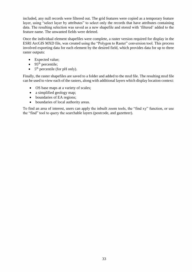
33

included, any null records were filtered out. The grid features were copied as a temporary feature

layer, using “select layer by attributes” to select only the records that have attributes containing

data. The resulting selection was saved as a new shapefile and stored with ‘filtered’ added to the

feature name. The unwanted fields were deleted.

Once the individual element shapefiles were complete, a raster version required for display in the

ESRI ArcGIS MXD file, was created using the “Polygon to Raster” conversion tool. This process

involved exporting data for each element by the desired field, which provides data for up to three

raster outputs:

Expected value;

95th percentile;

5th percentile (for pH only).

Finally, the raster shapefiles are saved to a folder and added to the mxd file. The resulting mxd file

can be used to view each of the rasters, along with additional layers which display location context:

OS base maps at a variety of scales;

a simplified geology map;

boundaries of EA regions;

boundaries of local authority areas.

To find an area of interest, users can apply the inbuilt zoom tools, the “find xy” function, or use

the “find” tool to query the searchable layers (postcode, and gazetteer).

34

5 Mapping appraisal and review

The risk maps are created to assess the spatial distribution of values for individual parameters

relative to the respective PCVs. It is anticipated that their utility will be in supporting decision

making on water-quality monitoring, and that they will be used in combination with existing

monitoring data for specific sites and specific site risk assessments, as part of the remit to fulfil

the objectives of Directive 2015/1787.

While every effort has been made to ensure the data are of high quality, the remaining uncertainties

with the data and with the maps produced need to be borne in mind when interpreting and

potentially making decisions on water-quality monitoring implications. Limitations are discussed

further below.

5.1 LIMITATIONS

5.1.1 Combining third-party data

The project relies on the combining of datasets from multiple sources. While this provides a

superior spatial coverage over any one individual dataset, there are complications associated with

using multiple data sources.

The inclusion of numerous detection limits means that statistical analysis needs to be handled

carefully using sophisticated statistical techniques. When mapping, a consensus on the detection

limit needs to be considered in order that spatial variation of detection limits is not mapped (see

Section 4.1.2), thus creating a false impression of the spatial variation. As these detection limits

generally occur at values <30% PCV, they did not pose a serious problem in this evaluation.

Various methods can be used to analyse the same parameter. While internal quality-control

methods are used before data are released, especially where laboratories have UKAS accreditation,

there may be differences in data released from various laboratories, especially between methods.

Of course, within individual datasets, different detection limits or methodologies may have been

used, especially if the project is long-running (e.g. G-BASE), the national scale involves different

laboratories being used (e.g. DWI’s PUB and PRI) or the dataset comprises numerous individual

projects (e.g. UKCEH). In such cases, however, there is commonly an internal quality-control

process to ensure the data are as comparable as possible.

5.1.2 Lack of information in the private water supplies data

The DWI’s PRI data were provided with the understanding that there were caveats to the quality

of aspects of the data, notably location. The exact nature of the problems was not understood until

the data had been explored. This is discussed above in Section 3.1.2.

The PRI data represent samples taken directly from the consumers’ taps. It was known that these

samples may therefore have been treated upstream of the sampling point. There are no metadata

describing such information, so it is unknown whether or not individual values represent treated

water, and if so, the type of treatment applied. The PRI data can therefore only represent a best

estimate of water-quality values. These data have been included in the geostatistically modelled

maps because private water supplies are commonly found in areas that are not served by mains

water, and therefore provide important information to fill the gaps in spatial distribution of sample

sites. The inclusion of these data and their associated caveats should be taken into consideration

when using the maps.

35

5.1.3 Zone classification

The original project proposal stated that waters would be classified into zones (e.g. aquifer, or type

of surface water). None of the groundwater data supplied by the third parties included metadata

on aquifer type or source depth, despite requests being made. On consideration of aquifers, the

best that could be achieved was an assessment of the surface geology at the sample point. This was

done using the BGS’s 1:625,000-scale solid and drift geology mapping (see Section 2.4). This

information cannot be assumed to correspond to the aquifer in all cases, as the aquifer may be

concealed beneath the surface geology, it may be unclear if the water is abstracted from the solid

or the drift geology, or the sample may be taken from one of a number of stacked aquifers. In areas

with groundwater derived from stacked aquifers (e.g. Chalk above Lower Greensand), the lack of

depth information in the dataset means that the mapping may present a mixture of aquifer

compositions, and so the true aquifer-specific variations may be represented inadequately. The

maps should be viewed with this limitation in mind.

The zone categories for the surface waters did not prove to be very useful. A total of 92% of the

surface-water sites were categorised as rivers or streams (22% rivers, 70% streams). The definition

of when a stream becomes a river is arbitrary so these definitions should be treated with caution.

Only 1% of the sites were classified as lakes, ponds or reservoirs, and the remaining 7% of the

sites were not categorised.

5.1.4 Decision making to flag out, change, or caution locations and data

As described in Sections 3.2 and 3.3, some of the locations and results were changed, flagged out,

or cautioned. Any changes from the original delivered data were made, based on expert judgement

with the aim of improving the quality of the dataset, and therefore the reliability of the produced

maps.

A limitation of the final dataset may be that original data have been changed unnecessarily, or any

unidentified errors were not changed and may remain within the dataset. As the majority of data

are third-party, and many with very limited associated metadata, we can never guarantee that all

data are correct as presented.

A further consideration is that data for the production of the risk maps were restricted to those

recorded since the start of 2015. This removed the contribution of older data and will therefore

have removed any influence they may have made to the spatial variations, probabilities and

associated uncertainty.

5.1.5 Sample coverage and areas of uncertainty

In areas where there are few sites (e.g. where groundwater is not used, or where few surface waters

flow), the maps have a greater uncertainty. A buffer has been set so that areas where there are no

data do not give a result. This is a function of natural datasets, and cannot be avoided. The spatial

distribution from each data source varied considerably:

The PUB and PRI databases comprised data which covered much of England and Wales.

There were more gaps within the PUB database as these represented the extraction of

waters for public consumption and hence the sites only occurred where there were major

aquifers or large rivers. The PRI sites are individual sources relating to one property or

group of properties, and therefore minor aquifers and aquifers with only local

significance are often used.

The EA and NRW datasets contained sites used for drinking water, as well as water

extracted for other uses (e.g. irrigation, manufacturing) and sites which were of

environmental interest. The EA dataset was by far the largest in terms of number of

results, and when combined with the NRW data there was a good coverage across

36

England (EA) and Wales (NRW) for both surface and groundwater. In recent years,

however, the number of sites sampled has reduced.

The sites within the G-BASE database were all low-order streams across England and

Wales. With a site every 1.5 km on average, this represented the best spatial coverage.

However, there were no groundwater samples. In addition each sample had been filtered,

meaning the metals data could not be combined with unfiltered metals data from other

datasets. These data also represented a one-off sample, which meant some of the data

were very old (from 1980) and there were no time series available. These data were thus

included in the exploratory data analysis summary statistics, but did not contribute to the

final risk map product.

The UKCEH data represented various individual studies. This means that the sites were

generally grouped in clusters and time-series data were limited. While the coverage was

patchy, the data did add value to reduce the uncertainty in some areas.

37

6 Recommendations

6.1 RECOMMENDATIONS TO EVALUATE THE PROCESS

Throughout the data cleaning and selection process, decisions had to be made on types of data to

use. Examples include use of filtered versus unfiltered analyses which amounts to whether to

incorporate dissolved or total concentrations; and whether to include all analyses (including some

older with high detection limits) or just more recent analyses. Unfiltered analyses were used in this

study as more data were available; the most recent analyses (post-2015 data) were also selected.

Decisions taken on sample selection would inevitably make some differences to the risk maps

produced and their associated uncertainties, and could potentially affect any decisions made on the

basis of them. Future modelling and mapping should consider data selection choices such as use

of all or most-recent data, or data from a 3-year period with maximum numbers of measurements;

filtered or unfiltered samples, for example.

6.2 RECOMMENDATIONS TO REVIEW THE PROCESS

There was a scarcity of sites with sufficient time-series data to be able to model expected future

concentrations with sufficient certainty (see Section 3.4), so maps of future projected

concentrations were not attempted. Instead, efforts were made to produce modelled expected and

percentile maps relevant to the current situation.

The trend maps produced as part of the exploratory data analysis (see Section 3.4.2) showed a lack

of systematic trends of increasing concentration for given parameters over large spatial scales.

There were disparate distributions for each, making it difficult to provide any consistent

recommendations for data review schedules. A repeat of the process described in this document

would be infeasible on a parameter-by-parameter basis. In the absence of any other guiding

principles, a recommended timescale for review of the processes undertaken for this investigation

to provide risk maps would be of the order of ten years, provided PCVs for individual parameters

do not change in the meantime. Changes to the PCV for any given parameter of course render any

affected static maps obsolete, but interactive maps in the GIS can be simply rescaled according to

the new PCV.

6.3 RECOMMENDATIONS TO IMPROVE THE PROCESS

As documented in this report, the project was delayed by various problems and unforeseen

complexities. In order to improve the process, a number of recommendations are provided below.

Error types identified in this study should be reiterated to data owners to cut down on

reproducing the errors in future. Examples include conventions for location recording and

for parameter units and formats and data censoring.

Recommendations for systematic recording of sampling purpose are appropriate.

Third parties should be advised to apply rules when adding data to their databases to

ensure that, for example:

o implausible values are not recordable (e.g. pH 67 instead of pH 6.7);

o new site locations do not plot in the incorrect 100 km grid square (including grid

references which should start with a “0”);

o existing sites are not accidentally given a unique name;

o existing sites retain the same grid reference; and

o new sites do not duplicate a site name.

Consideration should be given to dismissing third-party data from evaluations such as this

mapping exercise if effort to process them is disproportionate relative to the amount of data

provided. For example, small datasets produced by different groups in different formats may

38

require a disproportionate effort to clean and process for the quality and quantity of information

provided.

39

References

ANDERSON, C. W. 2005. Chapter A6, Section 6.7, Turbidity, Version 2.1. National Field Manual for the

Collection of Water Quality Data, US Geological Survey Techniques of Water Resources Investigators

Book 9. Reston, VA: U.S. Geological Survey.

BARDOSSY, A. 2002. Introduction to geostatistics. . Institute of Hydraulic Engineering University of Stuttgart,

Technical Note, p134.

HAYASHI, M. 2004. Temperature-electrical conductivity relation of water for environmental monitoring and

geophysical data inversion. Environmental Monitoring and Assesment, 96, 119-128.

HEM, J. D. 1992. Study and Interpretation of the Chemical Characteristics of Natural Water, Washington, United

StatesGovernment Printing Office.

ISO. 2016. Water quality — Determination of turbidity — Part 1: Quantitative methods.

https://www.iso.org/standard/62801.html [Online]. Available: https://www.iso.org/standard/62801.html

[Accessed].

LARK , R. M. 2015. Block correlation and the spatial resolution of soil property maps made by kriging. Geoderma,

295-260, 233-242.

LARK, R. M., CULLIS, B. R. & WELHAM, S. J. 2006. On spatial prediction of soil properties in the presence of a

spatial trend: the empirical best linear unbiased predictor (E‐BLUP) with REML. European Journal of Soil

Science, 57.

LEE, L. & HELSEL, D. 2005a. Nondetects And Data Analysis, New York, John Wiley and Sons.

LEE, L. & HELSEL, D. 2005b. Statistical analysis of environmental data containing multiple detection limits: S-

language software for regression on order statistics. Computers in Geoscience 31, 1241-1248.

LIM, K. F. 2006. Negative pH does exist. Journal of Chemical Education, 83, 1465.

MARCHANT, B. P. 2018. Model-based geostatistics. In: MCBRATNEY, A. B., MINASNY, B., STOCKMANN,

U. (ed.) A system of quantitative soil information. . Springer.

MARCHANT, B. P., VILLANNEAU, E. J., ARROUAYS, D., SABY, N. P. A. & RAWLINS, B. G. 2015.

Quantifying and mapping topsoil inorganic carbon concentrations and stocks: approaches tested in France.

Soil Use and Management, 31, 29-38.

MARCHANT, B. P., VISCARRA ROSSEL, R. & WEBSTER, R. 2013. Fluctuations in method of moments

variograms caused by clustered sampling and their elimination by declustering as residual maximum

likelihood. European Journal of Soil Science. European Journal of Soil Science, 64, 401-409.

NATIONAL WATER COUNCIL STANDING COMMITTEE OF ANALYSTS 1984. Colour and Turbidity of

Waters 1981. Methods for Examination of Waters and Associated Materials. London: HMSO.

NORDSTROM, D. K., ALPERS, C., N, PTACEK, C. J. & BLOWES, D. W. 2000. Negative pH and extremely

acidic mine waters from Iron Mountain, California. Environmental Science and Technology, 34, 254-258.

PEBESMA, E. 2018. Simple Features for R: Standardized Support for Spatial Vector Data. The R Journal 10, 439-

446.

VILLANNEAU, E., SABY, N. P. A., MARCHANT, B. P., JOLIVET, C. C., BOULONNE, L., CARIA, G.,

BARRIUSO, , E., B., A., , BRIAND, O. & ARROUAYS, D. 2011. Which persistent organic pollutants can

we map in soil using a large spacing systematic soil monitoring design? A case study in Northern France.

Science of the Total Environment, 409, 3719-3731.

WEBSTER, R. & OLIVER, M. A. 2007. Geostatistics for Environmental Scientists (second ed.), Chichester., John

Wiley & Sons, .

WICKHAM, H. 2016. ggplot2: Elegant Graphics for Data Analysis, Springer-Verlag New York.

WSI. 2018. Water, England and Wales. The Water Supply (Water Quality) Regulations 2018. Statutory Instrument

2018 No. 647 (W121) [Online]. Available:

http://www.legislation.gov.uk/wsi/2018/647/pdfs/wsi_20180647_en.pdf [Accessed July 2019].