risk management lessons from the global financial crisis

INDIAN INSTITUTE OF MANAGEMENTAHMEDABAD INDIA

Research and Publications

Risk Management Lessons from the Global Financial Crisis for Derivative Exchanges

Jayanth R. Varma

W.P. No.2009-02-06 February 2009

The main objective of the working paper series of the IIMA is to help faculty members, research staff and doctoral students to speedily share their research findings with professional colleagues and test their research findings at the pre-publication stage. IIMA is committed to

maintain academic freedom. The opinion(s), view(s) and conclusion(s) expressed in the working paper are those of the authors and not that of IIMA.

INDIAN INSTITUTE OF MANAGEMENT AHMEDABAD-380 015

INDIA

IIMA INDIA Research and Publications

W.P. No. 2009-02-06 Page No. 2

Risk Management Lessons from the Global Financial Crisis

for Derivative Exchanges

Jayanth R. Varma *

Abstract

During the global financial turmoil of 2007 and 2008, no major derivative clearing house

in the world encountered distress while many banks were pushed to the brink and beyond.

An important reason for this is that derivative exchanges have avoided using value at

risk, normal distributions and linear correlations. This is an important lesson. The global

financial crisis has also taught us that in risk management, robustness is more important

than sophistication and that it is dangerous to use models that are over calibrated to

short time series of market prices. The paper applies these lessons to the important

exchange traded derivatives in India and recommends major changes to the current

margining systems to improve their robustness. It also discusses directions in which

global best practices in exchange risk management could be improved to take advantage

of recent advances in computing power and finance theory. The paper argues that risk

management should evolve towards explicit models based on coherent risk measures (like

expected shortfall), fat tailed distributions and non linear dependence structures

(copulas).

_________________ * Professor Jayanth R. Varma, Indian Institute of Management, Ahmedabad 380 015, India. Email: [email protected]


W.P. No. 2009-02-06 Page No. 3

Risk Management Lessons from the Global Financial Crisis for Derivative Exchanges*

I. Derivative exchanges fared far better than banks

As in many other crises, during the global financial turmoil of 2007 and 2008 also, it was

true that no major derivative clearing house in the world encountered distress while many

banks were pushed to the brink and beyond. This was despite the fact that the exchanges

deal with more volatile underlyings – equities are about twice as volatile as real estate and

natural gas is about ten times more volatile than real estate. Clearly, risk management at

the world’s leading exchanges proved to be superior to that of the banks. The most

important lesson from the financial turmoil of 2007 and 2008 is that the quality of risk

management models does matter.

Exchanges and their clearing houses have weathered the storm very well thanks to their

superior risk management models. Yet, complacency is not warranted as exchanges start

trading more complex derivatives with asymmetric and lumpy payoffs.

Since the early 1990s, there have been three major advances in the theoretical foundations

of risk management:

1. abandoning Value at Risk (VaR) in favour of coherent risk measures like Expected Shortfall (ES);

2. moving away from the normal distribution to fatter tailed distributions; and

3. discarding linear correlations measures in favour of copula based models of tail dependence.

The cumulative effect of these three advances is so great that we must today regard the

risk measurement methodologies developed in the early 1990s as largely obsolete.

Banking regulations are however still stuck in the models of early 1990s vintage. What

we have seen in 2007 and 2008 is that VaR models based on normal distributions and

linear correlations models do not work.

The derivative exchanges have a huge advantage in that the SPAN1 system that most of

them use is a coherent risk measure unlike the VaR system used by banking regulators.

* © Prof. Jayanth R. Varma, Indian Institute of Management, Ahmedabad 380 015.

[email protected] 1 SPAN (Standard Portfolio Analysis of Risk) is a portfolio margining method developed by the

Chicago Mercantile Exchange in 1988. It calculates the portfolio loss under several price and volatility scenarios and determines the margin based on these loss levels.


W.P. No. 2009-02-06 Page No. 4

The SPAN risk measure can also be interpreted as an ES measure under certain

simplifying distributional assumptions. Additional layers of capital requirements and

other regulations might bring the exchanges’ risk models even closer to a realistic ES

measure.

Thus derivative exchanges have explicitly incorporated one of the three theoretical

advances of the last two decades. The other two advances may also be implicitly taken

into account by some exchanges. As the SPAN system does not explicitly specify how the

Price Scanning Range (PSR) is to be determined, exchanges are free to use fat tailed

distributions while deciding on the PSR. Moreover, exchanges are usually quite

conservative in fixing margin offsets for inter-commodity spreads. They may implicitly

treat linear correlations with a pinch of salt while deciding on these offsets. The very

success of the derivative clearing corporations world wide suggests that they have

implicitly factored in fat tails and non linear dependence structures at least to some

extent.

The global turmoil has also demonstrated the benefits of robust risk models. There is a

great difference between risk management models and valuation models. By their very

nature, valuation models need to be heavily parametrized and calibrated to market prices.

Increasing sophistication and complexity does lead to greater model risk, but this is

unavoidable, because trading at even slightly wrong prices can be disastrous for a

financial intermediary.

Risk management models on the other hand do not need to be so highly calibrated and

parametrized. Crudeness (leaning towards conservatism) is less of a problem in risk

management because unlike in valuation, here it only locks up capital for some time; it

does not impact the transaction price itself. Robustness is far more important than

sophistication and market calibration for risk management models.

Another important lesson from the ongoing Global Financial Crisis is that models

calibrated to short time periods from a benign economic environment can fail disastrously

when the economic environment becomes more adverse. While stress tests could be part

of the solution to this problem, a more fundamental approach is to calibrate to very long

time periods even if such a time period cuts across one or more structural breaks in the

data. What can be regarded as a structural break in a valuation model is often best

regarded as a regime switching in a risk management model – the implication being that

regime switches could reverse as well. Risk management is designed to deal with rare


W.P. No. 2009-02-06 Page No. 5

events, and the probability of such events can be estimated only by examining long

historical stretches of data.

Section II of this paper discusses VaR and ES models in greater detail; Section III

discusses the issues of robustness, regime switching and the associated question of risk

levels; Section IV discusses the implications of this analysis for some important

derivative markets in India. Section V is more speculative in nature as it considers

potential new advances in risk modelling techniques that are becoming feasible in the

light of continuing advances in mathematics and statistics as well as the relentless decline

in computation costs.

II. VaR, Coherent Risk Measures and Expected Shortfall

The 99% VaR at a daily horizon can be defined in the following different equivalent

ways2:

1. It is the level of capital that is sufficient to absorb the possible loss on 99% of the days.

2. It is the level of loss that is exceeded only on 1% of the days.

3. It is the worst of the best 99% of possible outcomes.

4. It is the best of the worst 1% of possible outcomes.

5. Unless the distribution has a hump in the tail, the 99% VaR is also the most likely of the worst 1% of possible outcomes.

The first two interpretations of VaR given above make VaR an intuitively appealing and

interesting summary measure of risk and account for its popularity among regulators,

managers and others.

The third and fourth interpretations of VaR highlight the serious difficulties with the

concept of VaR. For example, the fourth definition says that 99% VaR is essentially the

best of the worst 1% of outcomes. This immediately appears unsatisfactory – why not the

worst of the worst 1% of outcomes or at least the average of the worst 1% of outcomes?

It is easy to see that worst of the worst 1% is not a meaningful measure of risk because

the worst outcome may be unbounded. For example, a derivatives dealer that has sold a

2 These different definitions are equivalent if the loss distribution is continuous. If the distribution

is discrete or discontinuous, then these definitions may not all be equivalent. In this paper, the loss distribution is assumed to be continuous to keep the discussion simple.


W.P. No. 2009-02-06 Page No. 6

futures contract or sold a call option on a stock index faces potentially unlimited losses on

the position. There is no theoretical limit to how high the stock index can rise during the

life of the contract and the potential losses are therefore unbounded. The worst possible

outcome is thus ∞− (minus infinity). This is a meaningless measure of risk for most

practical purposes3.

The average of the worst 1% of possible outcomes is however a well defined and

meaningful measure of risk. In the risk literature, this is referred to as expected shortfall

(ES), conditional VaR (CVaR) or tail conditional expectation (TCE)4.

The distinction between VaR and ES is not very important if the loss distribution is

normal. For a normal distribution, the ES is ( )( )yN

yn−1

where y is the VaR. This is

asymptotically the same as VaR because ( ) ( )yyn=yN–

y1lim

∞→.

For non normal distributions, VaR can be quite different from ES. Consider for example

two securities firms that both have a one-day VaR of Rs 10 million at the 99% level. The

ES measure asks the question as to what happens on the 1% of days when the loss

exceeds Rs 10 million. It is possible that in one case, the loss ranges from Rs 10 million

to Rs 15 million with an average of Rs 12 million. In the other case, the loss may range

from Rs 10 million to Rs 20 million with an average of Rs 15 million. Clearly, the second

firm is a lot riskier than the first though both have the same VaR. The ES measure (Rs 15

million as compared to Rs 12 million) reveals this picture very well.

Though the average of the worst (ES) is a better measure of risk than the best of the worst

(VaR), VaR is very popular among financial institutions and their regulators. On the other

hand, no derivative exchange in the world uses VaR for margining purposes (Artzner et

al, 1999).

ES is the most important example of a coherent risk measure. Artzner et al (1999)

proposed four axioms for coherent risk measures:

3 It implies for example that a dealer that has sold one call option has the same level of risk as a

dealer that has sold a thousand call options. The worst possible outcome for both is minus infinity.

4 Strictly speaking these different terms are not identical if the loss distribution is discrete or discontinuous. However, as explained in footnote above, the loss distribution is assumed to be continuous throughout this paper.


W.P. No. 2009-02-06 Page No. 7

1. Translation invariance: Adding an initial sure amount to the portfolio reduces risk by the same amount.

2. Sub additivity: “Merger does not create extra risk”

3. Positive Homogeneity: Doubling all positions doubles the risk.

4. Monotonicity: Risk is not increased by adding position which has no probability of loss.

As already stated, ES is a coherent risk measure. The maximum of the expected loss

under a set of probability measures or generalized scenarios is also a coherent risk

measure. (Converse is also true). This implies that SPAN is coherent.

On the other hand, VaR is not coherent because it is not sub-additive. For example, one

day before maturity, a short call that has only a 0.75% chance of being exercised has zero

VaR because the probability of loss is less than 1%. Similarly, a short put that has only a

0.75% chance of being exercised also has zero VaR. However, a portfolio consisting of

the short call and the short put has a non zero VaR because there is a 1.5% chance that

one of the options will be exercised leading to a loss.

III. Robustness, Regime Switching and Risk Coverage Levels

Robustness

The margining benefits provided for calendar spreads or inter-commodity spreads in most

derivative exchanges globally is a good example of crude but robust models. Though

correlations are by no means constant, the spread margins or offsets are typically kept

constant for long periods of time. Moreover, they are set at levels that lead to over

margining of spread positions relative to what might be indicated by estimated

correlations. The big advantage is that the margining system is very robust in the face of

correlation breakdowns and correlation instability.

Exchanges have been able to use this robust system even in commodities (like energy)

where there is an active OTC market The higher margins induced by the robust system

have not led to a flight of the market to the OTC market where margin requirements could

perhaps be lower.

I hasten to add that it is the robustness and not the crudeness of the model that is the

virtue. A Luddite attack on sophisticated models is certainly warranted. I visualize

sophistication and robustness as orthogonal properties of risk management models. The


W.P. No. 2009-02-06 Page No. 8

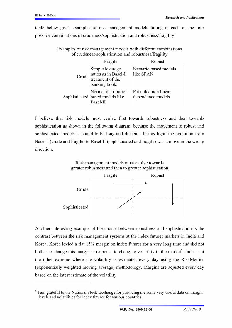
table below gives examples of risk management models falling in each of the four

possible combinations of crudeness/sophistication and robustness/fragility:

Examples of risk management models with different combinations of crudeness/sophistication and robustness/fragility

Fragile Robust

Crude

Simple leverage ratios as in Basel-I treatment of the banking book.

Scenario based models like SPAN

Sophisticated Normal distribution based models like Basel-II

Fat tailed non linear dependence models

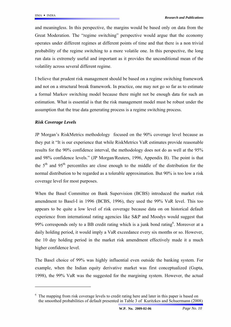
I believe that risk models must evolve first towards robustness and then towards

sophistication as shown in the following diagram, because the movement to robust and

sophisticated models is bound to be long and difficult. In this light, the evolution from

Basel-I (crude and fragile) to Basel-II (sophisticated and fragile) was a move in the wrong

direction.

Risk management models must evolve towards greater robustness and then to greater sophistication

Fragile Robust

Crude

Sophisticated

Another interesting example of the choice between robustness and sophistication is the

contrast between the risk management systems at the index futures markets in India and

Korea. Korea levied a flat 15% margin on index futures for a very long time and did not

bother to change this margin in response to changing volatility in the market5. India is at

the other extreme where the volatility is estimated every day using the RiskMetrics

(exponentially weighted moving average) methodology. Margins are adjusted every day

based on the latest estimate of the volatility. 5 I am grateful to the National Stock Exchange for providing me some very useful data on margin

levels and volatilities for index futures for various countries.


W.P. No. 2009-02-06 Page No. 9

Average margin levels in Korea are higher than in many other markets in the world –

even those markets (like India) where the average volatility is comparable. This excessive

level of margins provides very high protection against default. Yet, Korea has developed

one of the largest index futures markets in the world. What this shows is that a crude

model can provide adequate protection while not impeding market development.

It could be argued that the more “sophisticated” margining system in India is actually a

source of systemic risk for the exchange. If margins are revised at a frequency that

exceeds the ability of the payment system to mobilize funds from the ultimate client, then

large price movements can result in panic unwinding of levered positions that exacerbates

the original price movement. This can set up a vicious circle of accelerating volatility and

margin calls. There is anecdotal evidence to suggest that some of the extreme price

movements in recent years (particularly May 17, 2004 and January 21/22, 2008) have

witnessed this phenomenon. Bhalla (2008) makes this case very forcefully and

persuasively.

Regime Switching or Structural Breaks

One of the reasons why risk management in the global banking system failed so

miserably in 2007 and 2008 was because of reliance on historical data confined to the

“Great Moderation” during which macro-economic and systemic volatility was quite low.

Haldane (2009) provides the following data for macro-economic volatility in the UK:

Variable Volatility (1998-2007) Volatility (1857-2007) GDP growth 0.6% 2.7% Earnings growth 0.5% 6.4% Inflation 0.9% 5.9% Unemployment 0.6% 3.4%

Table 1: Volatility of UK macroeconomic variables during the Great Moderation compared with 150 year average. Source, Haldane (2009) Annex Table 1. We would all agree that margin levels should have been lower during the Great

Moderation than earlier. The question is whether the margins during this period should

have been based only on the observed volatility during this period or whether the margins

should also have been influenced by the past experience.

The “structural break” perspective would have argued that there was a structural

transformation in the economy in the late 1990s which made the earlier data irrelevant


W.P. No. 2009-02-06 Page No. 10

and meaningless. In this perspective, the margins would be based only on data from the

Great Moderation. The “regime switching” perspective would argue that the economy

operates under different regimes at different points of time and that there is a non trivial

probability of the regime switching to a more volatile one. In this perspective, the long

run data is extremely useful and important as it provides the unconditional mean of the

volatility across several different regime.

I believe that prudent risk management should be based on a regime switching framework

and not on a structural break framework. In practice, one may not go so far as to estimate

a formal Markov switching model because there might not be enough data for such an

estimation. What is essential is that the risk management model must be robust under the

assumption that the true data generating process is a regime switching process.

Risk Coverage Levels

JP Morgan’s RiskMetrics methodology focused on the 90% coverage level because as

they put it “It is our experience that while RiskMetrics VaR estimates provide reasonable

results for the 90% confidence interval, the methodology does not do as well at the 95%

and 98% confidence levels.” (JP Morgan/Reuters, 1996, Appendix B). The point is that

the 5th and 95th percentiles are close enough to the middle of the distribution for the

normal distribution to be regarded as a tolerable approximation. But 90% is too low a risk

coverage level for most purposes.

When the Basel Committee on Bank Supervision (BCBS) introduced the market risk

amendment to Basel-I in 1996 (BCBS, 1996), they used the 99% VaR level. This too

appears to be quite a low level of risk coverage because data on on historical default

experience from international rating agencies like S&P and Moodys would suggest that

99% corresponds only to a BB credit rating which is a junk bond rating6. Moreover at a

daily holding period, it would imply a VaR exceedance every six months or so. However,

the 10 day holding period in the market risk amendment effectively made it a much

higher confidence level.

The Basel choice of 99% was highly influential even outside the banking system. For

example, when the Indian equity derivative market was first conceptualized (Gupta,

1998), the 99% VaR was the suggested for the margining system. However, the actual

6 The mapping from risk coverage levels to credit rating here and later in this paper is based on

the smoothed probabilities of default presented in Table 3 of Kuritzkes and Schuermann (2008)


W.P. No. 2009-02-06 Page No. 11

risk containment system with a multiplicity of margin components (including longer

holding periods as well as additional components known variously as exposure margin,

second line of defence or extreme loss margin) delivered protection levels much higher

than 99%.

Basel-II credit risk models for the banking book in initial drafts (BCBS, 2001, para 172)

used 99.5% VaR levels corresponding to credit rating at the border line between BBB-

and BB+. The final Basel-II credit risk model (BCBS, 2004, para 272) is based on 99.9%

confidence level corresponding to a credit rating falling a little short of A-. In 2009, the

Basel Committee proposed that even in the trading book, credit risk should be based on

99.9% VaR levels (BCBS, 2009, para 12). All these credit risk VaR levels are over a one

year capital horizon.

For a derivative clearing corporation, I believe that margins should be based on a risk

coverage of about 99.95% with a one-day horizon. (As already indicated, the margins

should be based on expected shortfall and not on value at risk.) In terms of international

rating agency standards, 99.95% corresponds roughly to A levels while a clearing

corporation should be AAA rated. It would be necessary to rely on clearing corporation

capital, broker capital and other cushions to achieve AAA safety for the clearing

corporation while margins themselves provide only A level of safety.

It is doubtful whether it is possible to achieve AAA or even AA safety through margins

alone because a AA rating would have to be based on the 99.99% tail (and AAA would

require the 99.997% tail) and these extreme tails are not amenable to reliable statistical

estimation for fat tailed distributions.

In any case, exclusive reliance on margins is not a good idea. Since margins can be paid

out of borrowed funds, they do not constrain the overall leverage in the system. It only

ensures that when the excessive leverage leads to a failure, the losses fall on external

sources of leverage and not on the counter parties or on the exchanges. Leverage (whether

embedded or external) can be a source of systemic risk. A system of capital adequacy for

brokers and other intermediaries is an essential element of risk containment in the

derivative markets. Many analysts believe that weak capital adequacy systems for the

large broker-dealers (investment banks) contributed to the fragility of the financial system

in the United States in 2007 and 2008.


W.P. No. 2009-02-06 Page No. 12

IV. Risk Management in Indian Derivative Markets

Stock Index Futures

From the time they were introduced in the beginning of this decade, the Indian equity

derivative market has worked well without any serious defaults or settlement failures

despite large volumes and high levels of volatility. To this extent, the risk containment

system has worked quite well.

Nevertheless, there have been several serious concerns about the system:

It has been argued with some justification that the high frequency with which margins are revised is itself a source of systemic risk (Bhalla, 2008). This has been discussed in the previous section.

There has been a growing disconnect between the “Value at Risk” methodology to which the risk containment framework pays lip service and the actual system (modelled on SPAN) that is closer to modern coherent risk measures like “Expected Shortfall”.

The actual risk containment system with a multiplicity of margin components (including the 2 scaling as well as additional components known variously as exposure margin, second line of defence or extreme loss margin) delivers protection levels much higher than the 99% Value at Risk level enshrined in the stated regulatory goal.

Varma (2008) presented an alternative margining system to address the above concerns

based on analysis using data on the Nifty index for the period 1990-2008. The main

proposals can be summarized as follows:

It was proposed to set margins at a level equal to eight standard deviations corresponding to an expected shortfall measure at confidence level of 99.95%. This was to be in replacement of all margins and margin supplements levied currently including exposure margin or second line of defence or extreme loss margin as well the 2 scaling that is employed currently.

A minimum margin of 8% was proposed to prevent the margin from going too low during a “Great Moderation”. The current system also incorporates a minimum margin for the same reason.

It was proposed that margins (as a percentage of the underlying) would be revised only once a month and changes would be announced with sufficient notice to the markets. Specifically, the margin percentage for the next month would be based on data available on the 15th of the current month so that even after allowing for lags in computation and dissemination, it is possible to provide reasonable notice to the market.

To allow margins to be kept constant for such long periods, the volatility would be estimated with lower weight on the last few days of data and more weight on


W.P. No. 2009-02-06 Page No. 13

longer stretches of data. Specifically, the smoothing parameter (lambda in RiskMetrics/IGARCH) was proposed to be set to 0.995 as opposed to the 0.94 used currently7. The value of 0.995 was arrived at by quasi maximum likelihood estimation since this is known to be a consistent and robust estimator for GARCH type models even if the distributions have fat tails (Lee and Hansen, 1994).

Back-test results for the period August 1990 to August 2008 showed that margin

violations under the proposed system were well under control. In a sample of over 4,300

trading days, the 99.95% risk coverage requires a consideration of the worst 2 or 3 days.

The three largest moves in terms of number of standard deviations during the above

period were the following:

On May 17, 2004, the Nifty dropped 8.63 standard deviations (12.24%) in response to some market unfriendly remarks by leaders of the left parties whose support was needed for the incoming government.

The Nifty rose by 7.10 standard deviations (12.85%) on March 24, 1992 during the securities scam. After the exposure of the scam, the index had three moves of more than 10% during April and May 1992, but the volatility estimates by then were so high that these moves were less than six standard deviations.

The Nifty rose 6.96 standard deviations (10.44%) on March 1, 1997 in response to the “dream budget” the previous day .

The proposed margining system (eight standard deviations) is slightly in excess of what is

required to achieve an ES at the 99.95% level8. A margin level somewhere between 7½

and 8 standard deviations would be sufficient. The only margin violation is on May 17,

2004 where the index movement of 12.24% exceeded the margin of 11.34% by 0.90%.

The average margins and the range of margins are shown in Table 2. During the recent

period, the margins range from around 9% to around 16% with an average of about 12%.

The margins are higher in the more volatile 1990s.

7 Using a high value of λ means that the volatility estimate takes into account a much longer

period of historical data. When λ is 0.94, the most recent 11 days account for half the weights and the most recent 37 days account of 90% of the weights. When λ is raised to 0.995, the corresponding numbers are 138 days and 459 days. Therefore the effect of a wrong initial volatility estimate lasts for about 1-2 years when λ=0.995. On the other hand, with λ=0.94, the initial value affects the estimates only for the first month or so. It is proposed that when λ = 0.995 is used, the volatility estimates should be initialized on a date at least 3 years in the past so that the initial value has a negligible impact on the current volatility estimate.

8 The 99.95% VaR would require an even lower margin level (below seven standard deviations).


W.P. No. 2009-02-06 Page No. 14

Average, minimum and maximum margins 1990-2008 1996-2008 2001-08 Average 13.54% 12.71% 12.09%

Minimum Not meaningful9 9.02%(August 2003)

9.02% (August 2003)

Maximum 23.94%(June 1992)

16.85%(June 2000)

16.24% (May 2008)

Table 2: Average, minimum and maximum margins under the system proposed in Varma (2008) and recommended here as well A structural break perspective might argue that the bad old days of an unreformed capital

market of the early 1990s are irrelevant in today's environment. If so, a flat 12% margin

(Korean style) might be as good or better than the proposed system. It gives the same

level of protection with a lower level of average margins!

From a regime switching perspective, things look very different. In this perspective, there

is a non trivial probability that a change in the domestic or global economic environment

could take us back to the high volatility regime of 1992. The proposed margining system

is robust in the face of such a regime switch while a 12% flat margin would not be. Yes, a

15% flat margin would be robust even under a 1992 volatility regime, but that implies a

significantly higher average margin as the price of the greater simplicity.

Currency Derivatives

When exchange traded currency derivatives were introduced in India, the risk

management system for these products was implicitly drawn from the system used for

equity derivatives (Reserve Bank of India and Securities and Exchange Board of India,

2008). This is in my view a cause for concern because currencies are an ill behaved asset

class compared to equities.

First, equities have relatively well defined fundamentals. Second, to a fair approximation,

equity prices are market clearing prices so that the observed volatility of equity prices

captures all relevant information about the volatility of supply and demand. Exchange

rates by contrast have poorly defined fundamentals; purchasing power parity is the closest

that we have to the fundamentals for exchange rates, but deviations from these

fundamentals take several years to correct themselves (Lothian and Taylor, 1996).

Moreover, exchange rates are not often market clearing prices because of large scale 9 Since the margin computations were started off from an artificially low level in July 1990, the

margins in the first month are low (about 8%), but this is a meaningless number.


W.P. No. 2009-02-06 Page No. 15

central bank intervention. As such, highly volatile supply and demand can co-exist with

low observed volatility of exchange rates.

The problem is that at some point of time, the central bank might decide to abandon its

exchange rate stabilization policy and thus cause a large jump in the exchange rate in

either direction. This is of course the well known peso problem in exchange rate theory.

The point is that the volatility estimated from past exchange rates contains no information

relevant to the peso problem risk. When the jump materializes, it appears as a bolt from

the blue to a GARCH or IGARCH risk model.

The jump might be less of a surprise to a model that tracks the volatility of reserves in

addition to the volatility of exchange rates themselves. Even here, however, the timing of

the jump would come as a surprise though the direction and magnitude of the jump might

be less surprising.

I believe that measured exchange rate volatility is a poor measure of the true risk of

currency derivatives. In particular, GARCH and IGARCH models perform quite badly in

the rupee-dollar exchange rate (Varma, 1999). There are broadly two alternatives for risk

management of currency derivatives:

1. It is possible to have a flat margin that is completely unresponsive to currency market conditions. The rationale for such a system would be that currency risk is dominated by jump risk and this risk is unpredictable (at least in respect to the timing of the jump). The simplest robust margin system is one that assumes that a jump could happen at any time and imposes a margin that protects against a fairly large jump at all times. After the introduction of market determined exchange rates (LERMS) in March 1992, the most extreme percentage move in the rupee dollar rate was the 3% move on September 14, 1995. A flat margin set at this level would provide coverage at the 99.95% level over this period. From a regime switching perspective, however, one would worry about two things:

◦ The devaluation of the currency in mid 1991 and early 1992 during the transition to managed floating was several times this level.

◦ Other emerging market currencies comparable to India in terms of the size of the economy, the level of foreign exchange reserves and the quality of national leadership have witnessed much larger single day moves at times of crisis (for example, Korea in the last quarter of 2008).

2. It is possible to design a margining system that responds to the volatility of supply and demand as measured not only by exchange rate volatility but also the volatility of foreign exchange reserves and interest rates. Implied volatility of currency options (particularly risk reversals) might also provide valuable information. Risk management systems that take this approach would attempt to predict the timing of jumps and impose high margins only when the probability of jumps is quite high.


W.P. No. 2009-02-06 Page No. 16

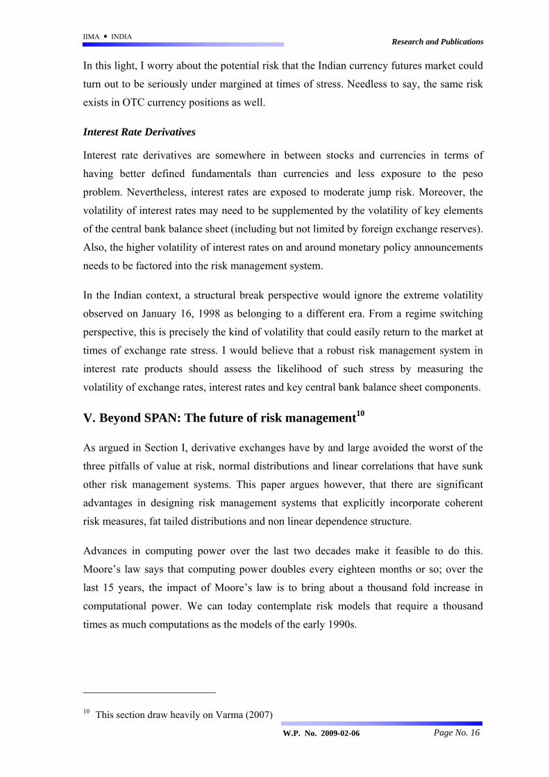
In this light, I worry about the potential risk that the Indian currency futures market could

turn out to be seriously under margined at times of stress. Needless to say, the same risk

exists in OTC currency positions as well.

Interest Rate Derivatives

Interest rate derivatives are somewhere in between stocks and currencies in terms of

having better defined fundamentals than currencies and less exposure to the peso

problem. Nevertheless, interest rates are exposed to moderate jump risk. Moreover, the

volatility of interest rates may need to be supplemented by the volatility of key elements

of the central bank balance sheet (including but not limited by foreign exchange reserves).

Also, the higher volatility of interest rates on and around monetary policy announcements

needs to be factored into the risk management system.

In the Indian context, a structural break perspective would ignore the extreme volatility

observed on January 16, 1998 as belonging to a different era. From a regime switching

perspective, this is precisely the kind of volatility that could easily return to the market at

times of exchange rate stress. I would believe that a robust risk management system in

interest rate products should assess the likelihood of such stress by measuring the

volatility of exchange rates, interest rates and key central bank balance sheet components.

V. Beyond SPAN: The future of risk management10

As argued in Section I, derivative exchanges have by and large avoided the worst of the

three pitfalls of value at risk, normal distributions and linear correlations that have sunk

other risk management systems. This paper argues however, that there are significant

advantages in designing risk management systems that explicitly incorporate coherent

risk measures, fat tailed distributions and non linear dependence structure.

Advances in computing power over the last two decades make it feasible to do this.

Moore’s law says that computing power doubles every eighteen months or so; over the

last 15 years, the impact of Moore’s law is to bring about a thousand fold increase in

computational power. We can today contemplate risk models that require a thousand

times as much computations as the models of the early 1990s.

10 This section draw heavily on Varma (2007)


W.P. No. 2009-02-06 Page No. 17

Coherent Risk Measures

In addition to the four core axioms defining coherence, Artzner et al also proposed an

Axiom of Relevance: “Position that can never make a profit but can make a loss has

positive risk”. For scenario based measures, the requirement can be stated differently as

requiring consideration of a Wide Range of Scenarios: “Convex hull of generalized

scenarios should contain physical and risk neutral probability measures.”

Though, SPAN is a coherent risk measure, it does not satisfy this additional requirement

because in my opinion, it has too few scenarios. For example, if the price scanning range

is set at ±3σ, then there are no scenarios between 0 and σ which covers a probability of

34% under the normal distribution.

To see the difficulties that this creates, consider a short butterfly (two long calls close to

the money and two short calls – one at a higher strike and the other at a lower strike). This

portfolio loses the maximum money when the underlying is close to the strike of the long

calls – this is due to the decay of the option premiums of these long calls. If all the strikes

are close together, it is possible for this maximum loss to occur at a point in between two

SPAN scenarios and the SPAN risk measure underestimates the true loss as seen in

Figure 1.


W.P. No. 2009-02-06 Page No. 18

There are two possible solutions to the problem of non linear positions that have large losses in between two scenarios:

1. We can increase the number of scenarios. If the risk is defined in terms of the worst 1% outcomes (99% VaR or ES), it would make sense to have a scenario at each percentile of the distribution of the underlying. With today’s computational power, this increase in the number of scenarios is eminently affordable. If risk is defined at higher coverage levels (99.95% VaR or ES), the increase in the number of scenarios can prove challenging.

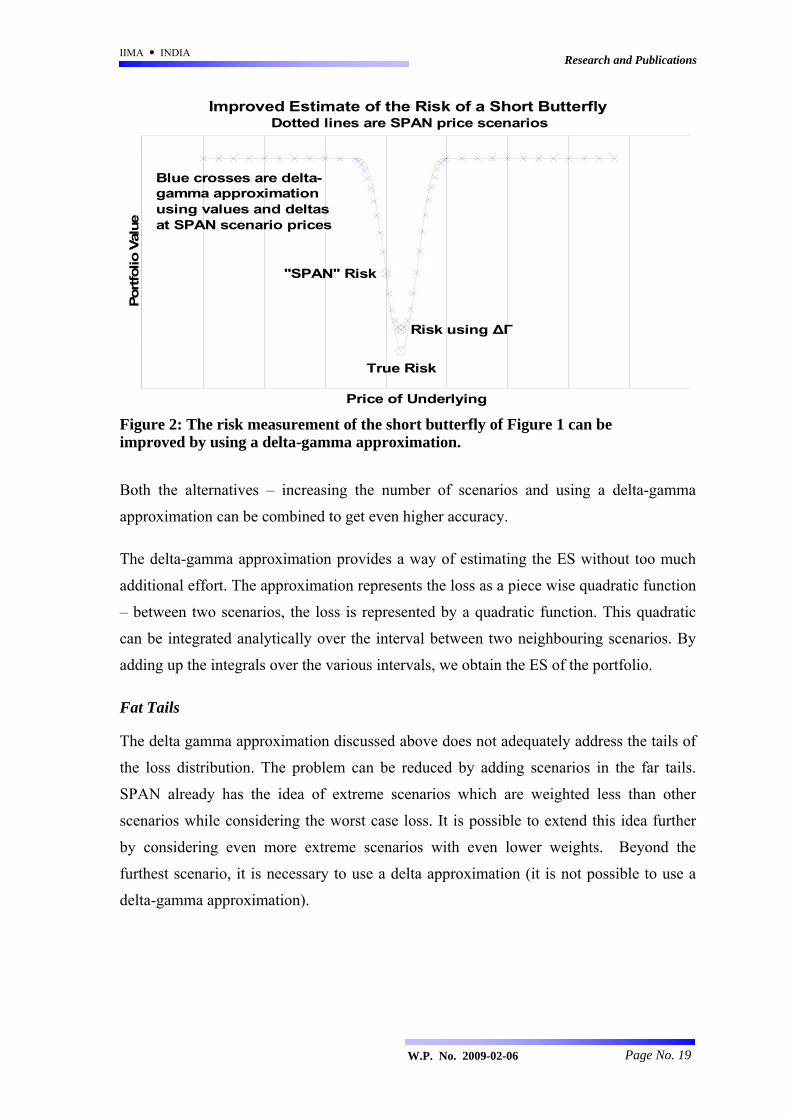
2. With the same set of scenarios, we can estimate the risk of option positions better by using a delta-gamma approximation. The portfolio values and deltas at neighbouring scenarios allows the gamma of the portfolio to be estimated. The delta-gamma approximation is equivalent to fitting a quadratic curve that passes through the scenario points. The maximum loss under this quadratic curve can be determined analytically without computing any additional scenarios. This is shown in Figure 2.

SPAN Underestimates the Risk of a Short ButterflyDotted lines are SPAN price scenarios

"SPAN" Risk

True Risk

Price of Underlying

Port

folio

Val

ue

Figure 1: The true risk is significantly higher than the risk as measured by SPAN for a short butterfly (two long calls close to the money and two short calls – one at a higher strike and the other at a lower strike). This portfolio loses the maximum money when the underlying is close to the strike of the long calls. In this diagram, the central strike falls between two scenarios and the other strikes are close to these scenarios. The maximum loss occurs at a price between two scenarios.


W.P. No. 2009-02-06 Page No. 19

Both the alternatives – increasing the number of scenarios and using a delta-gamma

approximation can be combined to get even higher accuracy.

The delta-gamma approximation provides a way of estimating the ES without too much

additional effort. The approximation represents the loss as a piece wise quadratic function

– between two scenarios, the loss is represented by a quadratic function. This quadratic

can be integrated analytically over the interval between two neighbouring scenarios. By

adding up the integrals over the various intervals, we obtain the ES of the portfolio.

Fat Tails

The delta gamma approximation discussed above does not adequately address the tails of

the loss distribution. The problem can be reduced by adding scenarios in the far tails.

SPAN already has the idea of extreme scenarios which are weighted less than other

scenarios while considering the worst case loss. It is possible to extend this idea further

by considering even more extreme scenarios with even lower weights. Beyond the

furthest scenario, it is necessary to use a delta approximation (it is not possible to use a

delta-gamma approximation).

Improved Estimate of the Risk of a Short ButterflyDotted lines are SPAN price scenarios

"SPAN" Risk

Risk using ∆Γ

True Risk

Price of Underlying

Port

folio

Val

ue

Blue crosses are delta-gamma approximation using values and deltas at SPAN scenario prices

Figure 2: The risk measurement of the short butterfly of Figure 1 can be improved by using a delta-gamma approximation.


W.P. No. 2009-02-06 Page No. 20

In addition, it is convenient to assume that the tail follows a power law11. In this case, ES

can be approximated12 in the tails using the tail index: VaRh

h=ES1−

.

With this approximation, we have a robust risk measure (approximate ES) that satisfies

the core axioms of coherence as well as the axiom of relevance.

Multiple Underlyings: Correlations and Copulas

Derivative exchanges have used a very conservative approach to the problem of

correlations. SPAN simply aggregates margins across underlyings without any benefit

for diversification and portfolio hedges. The only exception is that it provides some

margin offsets for inter commodity spreads in closely related underlyings. This very

conservative approach has helped derivative exchanges to weather many financial crises

without serious distress.

Banking regulators on the other hand allow banks to uses correlations and assume

multivariate normality to compute the portfolio risk with full benefit of diversifications

and portfolio hedges. During periods of turmoil, however, correlation are often unstable

and the assumed diversification benefits may disappear. Extreme price movements are

more correlated than usual (for example, crash of 1987, dot com bubble of 1999 and the

turmoil of 2007-08). It is not possible to protect the exchange simply by assuming a

higher correlation than the historical average. This is because low correlation under

margins long-only portfolios while high correlation under margins long-short portfolios.

Therefore instability of correlations in either direction can be dangerous for the risk

managers.

Instability is difficult to model because if correlations vary over time, historical data

becomes less useful to estimate the dependence. A different perspective has however

gained ground in recent years. This is the view that the dependence between two

underlyings is stable but non linear. Non linear dependence can account for the high

correlation of extreme movements and the modest correlation of mild movements. It can

also account for asymmetric dependence relationships where the dependence is different

in rising and falling markets. Correlations are a poor measure of non linear dependence.

11 The normal distribution has exponentially declining tails – the density is proportional to e− x2

2 .

Fat tailed distributions have tails that decline more slowly. The density is proportional to x− h

where h is the tail index.

12 This approximation is used implicitly in the second line of defence in the margining system of Indian exchange traded derivatives (Varma, 2002, Section 4.1).


W.P. No. 2009-02-06 Page No. 21

For example if x lies between –1 and +1 and 2x=y , then x and y are uncorrelated though

y is perfectly dependent on x.

Copulas provide the mathematical machinery to model non linear dependence. They are

the way to go to measure risk at a portfolio level without relying on ad hoc margin

offsets.

The gaussian copula postulates a linear relationship between two variables. If the

correlation is zero then the two variables are unrelated. This is shown in the scatter

diagram in Figure 3 which presents a circular pattern. There are hardly any instances of a

simultaneous extreme movement in both variables. It is well known that the gaussian

copula implies negligible tail dependence.

Figure 3: The gaussian copula with zero correlation produces a scatter plot which is circular. There are very few observations involving simultaneous extreme moves of both x and y.


W.P. No. 2009-02-06 Page No. 22

This must be contrasted with the non linear dependence of the t-copula shown in Figure 4.

Here also the correlation is zero signifying the absence of a linear relationship. The two

variables are individually normally distributed as in the earlier diagram. However, there is

a non linear dependence. The scatter plot looks like a square and simultaneous extreme

movements in both variables are seen. If we were modelling the relationship using

correlations, then in times of market stress, it would appear that two previously

uncorrelated variables have become highly correlated. In fact, the dependence

relationship has been stable but was non linear to begin with.

Multivariate normality (the gaussian copula) is computationally very attractive – it solves

the curse of dimensionality as the portfolio distribution is univariate normal. To retain

computational tractability, the use of a unidimensional mixture of multivariate normals is

attractive as it reduces to numerical integral in one dimension. With modern

Figure 4: A t-copula with zero correlation produces a scatter diagram which looks like a square rather than a circular. The tail dependence is seen in simultaneous extreme moves in both x and y


W.P. No. 2009-02-06 Page No. 23

computational power a univariate numerical integration in one dimension is quite

feasible.

This makes multivariate t (t copula with t marginals) very attractive as it is an inverse

gamma mixture of multivariate normals. Other univariate mixtures are possible.

To use copulas, we must fit a marginal distribution to the portfolio losses for each

underlying and apply the copula to these marginals. SPAN with enough scenarios allows

us to approximate the distribution. If we wish to fit a distribution from a parametric

family of distributions, it is essential that we fit the distribution to match the tails well.

This implies that we must match tail quantiles in addition to matching moments.

The Adverse Selection Problem

The clearing corporation provides a service similar to that of insurance and the concept of

adverse selection is applicable to it as well. In this context, the margins imposed by the

clearing corporation play a role similar to the premium charged by insurance companies.

Adverse selection therefore implies that positions that are under-margined would be

heavily used while those that are over-margined would be less popular. Even if the

margins were right on average for randomly chosen positions, they would be too low for

the actual positions chosen by traders.

Adverse selection arises essentially because as emphasized in the limits to arbitrage

literature, arbitrage is often constrained by leverage. Arbitrageurs therefore seek under-

margined portfolios.

We can think of this as a two stage game:

Exchange moves first – announces the SPAN scenarios

Arbitrageur moves second – chooses portfolios

The interesting question is whether we can reverse this order of moves. Can the scenarios

be tailored to the portfolio in a transparent pre-announced fashion. For example, the

exchange might say that it would add scenarios at prices corresponding to the five strikes

at which option positions are most heavily concentrated.

On deeper thought, it is not necessary to really do this on a portfolio by portfolio basis.

Defaults by a few traders is not damaging to the exchange. What is critical is large scale

or systemic defaults. The exchange (or its clearing corporation) is short options on each

trader’s portfolio with strike equal to portfolio margin. The position of the clearing house


W.P. No. 2009-02-06 Page No. 24

is thus a portfolio of such short options. One can then ask the question: What price

scenarios would create the worst loss to exchange (aggregated across all traders)? The

exchange can then add these scenarios to the margining system dynamically.

The determination of the worst loss scenarios might appear to be the same as stress

testing, but it is actually an “inverse problem.” Instead of starting with specified scenarios

and finding the loss under these scenarios, the idea is to specify an extreme loss level and

determine the most likely scenario that could lead to this loss. Fournie, Lasry and Lions

(1997) present some promising ideas on solving a similar problem by computing

Finslerian geodesic paths.

VI. Conclusion

Derivative exchanges have fared much better banks during the global financial crisis as

their models were more robust even if they appeared crude in comparison to the internal

models of the large banks. This is an important lesson and risk managers must continue to

emphasize robustness in their models. Sophistication and market calibration should never

be pursued at the cost of robustness.

However, it would be a mistake for exchanges to become complacent about their

margining systems. Risk management is a rapidly evolving field with new methods being

developed constantly. Growing computational power is also making previously infeasible

approaches increasingly practicable. Risk managers must be continually striving to adopt

the best models that are both robust and computationally tractable.

Derivative exchanges in India need to look carefully at their margining methodology and

eliminate certain elements that could contribute to the fragility of the risk management

system. Specific recommendations have been given in the paper about stock index futures

and currency futures. Similar analyses have to be performed about other derivative

products as well.


W.P. No. 2009-02-06 Page No. 25

References

Artzner et al (1999), “Coherent Measures of Risk”, Mathematical Finance, 9(3), 203-228

Basel Committee on Banking Supervision (BCBS) (1996) “Amendment to the capital accord to incorporate market risks”, Bank for International Settlements.

Basel Committee on Banking Supervision (BCBS) (2001) “Consultative Document: The Internal Ratings-Based Approach. Supporting Document to the New Basel Capital Accord”, Bank for International Settlements.

Basel Committee on Banking Supervision (BCBS) (2004) “International Convergence of Capital Measurement and Capital Standards: A Revised Framework”, Bank for International Settlements.

Basel Committee on Banking Supervision (BCBS) (2009), “Guidelines for computing capital for incremental risk in the trading book”, Bank for International Settlements.

Bhalla, Surjit S (2008) “The ultimate crisis machine – Sebi’s risk management”, Business Standard, January 26, 2008.

Fournie, E; J Lasry and PL Lions (1996) “Some nonlinear methods to study far-from-the-money contingent claims” in Rogers, L. C. G. and Denis Talay (ed) Numerical Methods in Finance, Cambridge University Press.

Gupta LC (Chairman) (1998), “Report of the Committee on Derivatives”, Securities and Exchange Board of India.

Haldane , Andrew G (2009), “Why banks failed the stress test”, Bank of England, www.bankofengland.co.uk/publications/speeches/2009/speech374.pdf

JP Morgan/Reuters (1996) “RiskMetrics Technical Document”

Kuritzkes, A. and T. Schuermann (2008), “What we know, don’t know and can’t know about bank risk: a view from the trenches”, http://papers.ssrn.com/sol3/papers.cfm?abstract_id=887730

Lee, S W and Hansen, B E (1994) “Asymptotic theory for the GARCH (1,1) quasi-maximum likelihood estimator”, Econometric Theory, 10, 29-52.

Lothian, J. R. and Mark P. Taylor (1996), “Real exchange rate behaviour: The recent float from the perspective of the past two centuries”, Journal of Political Economy, 104(3), 488-509.

Reserve Bank of India and Securities and Exchange Board of India (2008) “Report of the RBI-SEBI standing technical committee on exchange traded currency futures”

Varma, J R (1999) “Rupee-Dollar Option Pricing and Risk Measurement: Jump Processes, Changing Volatility and Kurtosis Shifts”, Journal of Foreign Exchange and International Finance, 1391), 11-33

Varma, J R (Chairman) (2002) “SEBI Advisory Committee on Derivatives: Report on the development and regulation of derivative markets in India”, Securities and Exchange Board of India.


W.P. No. 2009-02-06 Page No. 26

Varma, J R (2007) “Risk Management at Indian Exchanges: Going Beyond Value at Risk”, Seminar at Indian Council for Research on International Economic Relations , January 9, 2007.

Varma, J R (2008) “Note on revising the margining of stock index futures in India”, mimeo, August 2008, revised September 2008.

risk management lessons from the global financial crisis

Documents