Risk Disaggregation As An Explanation Of TheSmile : The Black & Scholes Formula Revisited.

Thierry Chauveau¤ Hayette Gatfaouiy

September 2001

¤TEAM Pôle Finance (ESA 8059 du CNRS) of the University Paris I - Panthéon-Sorbonne,Maison des Sciences Economiques, 106-112, boulevard de L’Hôpital, 75013 Paris. Email :chauveau@univ-paris1.fr

yTEAM Pôle Finance (ESA 8059 du CNRS) of the University Paris I - Panthéon-Sorbonne,Maison des Sciences Economiques, 106-112, boulevard de L’Hôpital, 75013 Paris. Email :gatfaoui@univ-paris1.fr

1

Résumé

Dans leur formule, Black & Scholes évaluent le prix d’un call européenportant sur un actif sous-jacent sans distinction des risques qui composent cedernier. En appliquant la méthode de pricing de Black & Scholes tout en faisantla distinction, à l’image de Sharpe (1964), entre le risque de marché et le risqueidiosyncratique, nous obtenons une nouvelle formule de pricing de call européen.Les paramètres de cette formule comprennent les volatilités des deux facteurs derisque ou, de façon équivalente, la volatilité du facteur de marché ainsi que cellede l’action sous-jacente. Nous construisons alors un portefeuille destiné à du-pliquer le facteur de marché, ce portefeuille de réplication étant un portfeuillediversi…é de façon naïve. Sous certaines conditions de régularité, l’e¤et de di-versi…cation connu pour compenser les risques spéci…ques, s’applique. Le prixd’un call européen portant sur une action peut alors s’exprimer en termes desvolatilités respectives du portefeuille de réplication et de l’action sous-jacente(ainsi que de son beta). Finalement, nous comparons notre formule à celle deBlack & Scholes ainsi qu’à la méthode d’évaluation proposée par Corrado & Su.Nous mettons en évidence l’existence d’un smile de volatilité tout en fournissantune explication concurrente de celle proposée par les modèles à volatilité stochas-tique (i. e : Heston [1993]) ou par les modèles supposant une distribution nonnormale pour les rendements des actifs (i. e : Corrado & Su [1996, 1997]).

Mots clés : évaluation d’option, smile de volatilité, risque systématique, risqueidiosyncratique, diversi…cation.

Abstract

In their formula, Black & Scholes evaluate a european call on an underly-ing asset without distinguishing between the di¤erent risks borne by the asset.Applying the Black & Scholes’ pricing methodology and distinguishing betweenthe market risk and idiosyncratic risk, as Sharpe [1964] did, we obtain a newpricing formula for a european call. The parameters of this formula include thevolatilities of the two risk factors, or alternatively, the volatility of the marketfactor and that of the stock. We then build a market factor replicating portfolio(MFR) which is a naively divesi…ed portfolio. Under some regularity conditions,the diversi…cation e¤ect known to o¤set the speci…c risks applies. The price ofa european call on a stock may then be expressed in terms of the volatilities ofthe MFR portfolio and of the underlying stock (and of its beta). Finally,wecompare our formula to that of Black & Scholes and to the valuation proposedby Corrado & Su. We focus on the existence of a volatility smile and we give anexplanation competing with the one proposed by stochastic volatility models (e.g. Heston [1993]) or models assuming a non normal distribution for the assets’returns (e. g. Corrado & Su [1996, 1997]).

Keywords : option pricing, volatility smile, systematic risk, idiosyncratic risk,diversi…cation.JEL Codes : G11, G12, G13.

2

1 IntroductionThe most famous concept of market equilibrium is that of the Capital Asset

Pricing Model (henceforth CAPM). It was developed almost simultaneously bySharpe [1963,1964], and Treynor [1961]1. The major result given by the CAPMis that the total risk of an individual asset can be partitioned into two parts :systematic risk which is a measure of how the asset covaries with the economyand unsystematic risk which is independent of the economy. More precisely, anyof the n traded risky assets exhibits an expected return which depends linearlyon the level of a common factor –the market factor– and that of an independentidiosyncratic risk2. Such a point of view implies that, if time were allowed tovary explicitly3, the dynamics of the n risky assets would be driven by that ofn+1 independent factors. Consequently, this type of model is inconsistent withthe complete market hypothesis underlying the …nancial assets valuation …rstproposed by Black & Scholes [1973].

One could argue that such an inconsistency vanishes if one considers moresophisticated versions of the CAPM such as the one developped by Merton[1973] in which it is assumed that trading takes place continuously and thatasset returns are distributed log-normally. If the risk-free rate of interest isnon stochastic over time, the equilibrium returns must then satisfy an equationanalogous to that of the elementary CAPM4. However, the dynamics of the ntraded risky assets is determined by that of n independent factors. Hence, themarket is complete and the return on the market portfolio is a linear combinationof those of the n independent factors. The CAPM and Black and Scholes’valuation formula are compatible. Nevertheless, if the major result exhibited bythe CAPM still holds when Merton’s assumptions are made, its interpretationis very di¤erent from the original one. Strictly speaking, there is no longer anymarket factor.

One could also argue that, in later works dealing with arbitrage pricing, thecomplete market hypothesis has often be relaxed5. However, in almost all thesestudies, the market risk has still to be de…ned as a combination of individualrisks.

To reconcile the “traditional view” –which we shall call Sharpe’s approach–with the valuation proposed by Black & Scholes, we develop a two-factor modelassuming that the price of any traded stock depends on the level of the marketrisk and of that of a speci…c risk; the levels of the two factors are assumed tobe two independent geometric brownian motions. We then use such a risks’disaggregation for option pricing.

This paper is organized as follows. Using a complete …nancial market frame-work, we …rst address the issue of valuing an option whose underlying asset is

1 Extensions of the model were provided by Mossin (1966), Lintner (1965,1969) and Black(1972) .

2 There are thus as many speci…c risks as there are assets.3 Which is not ususally the case when elementary versions of the CAPM are under review.4 To spare space, we leave aside the case when the risk-free interest rate is stochastic and,

consequently, when the model exhibits two risk factors (and, therefore, three-fund separation).5 For further details, see Cochrane & Saa-Requejo (1998) and Pham (1998).

3

a stock, given that the price of the stock is assumed to be determined by twoindependent risk factors, namely a market risk (common to all the stocks) andan idiosyncratic risk respectively6. It is easy to obtain an analytical formulafor valuing european calls on stocks if it is further assumed that not only then stocks but also the (n + 1) factors are traded. The same result is obtainedunder the weaker assumption that only the n stocks and the market factor aretraded. In this case, the price of an option is no longer expressed in terms ofthe volatilities of the market factor and of the pertinent idiosyncratic factor butin terms of the volatility of the market factor and that of the underlying asset.

Second, we take into account the diversi…cation e¤ect to get rid of the un-observability of the market factor. If the number of assets is high enough –andparticularly if it tends towards in…nity–, we can build a diversi…ed portfoliowhose value is as close to that of the market portfolio as we want. The simulta-neous observation of the portfolio’s value and the prices of the n quoted assetsis then equivalent to those of the n stocks and of the level of the market factor.In this case, the price of an option may be expressed in terms of the volatility ofa naively diversi…ed market portfolio and that of the underlying asset. Optionpricing remains possible even if none of the factors is tradable –which is the casein practice–.

Finally, we compare our pricing to that of Black & Scholes [1973] and ofCorrado & Su ([1996, 1997]), using a simulation method. This framework allowsus to focus on the existence of a volatility smile; we then give an explanationcompeting with the one proposed by stochastic volatility models (e. g. Heston[1993]) or models assuming a non normal distribution for the assets’ returns (e.g. Corrado & Su [1996, 1997]).

2 Option pricing with two factors : reconcilingSharpe’s and Black & Scholes’ points of view.

In this section, we use the framework of Black & Scholes [1973] except thatthe price of the underlying asset does no more depend on a unique risk factorbut on two risk factors.

Assumptions :

We consider the price St of a stock : it is an Ft-adapted process whereFt represents the available information contained in the stock’s price at thecurrent date t. We suppose that the dynamic of St depends both on a marketrisk factor whose level is labelled Xt and on an idiosyncratic risk factor whosevalue is denoted It. The former represents a risk associated to the economic

6 The complete market hypothesis is equivalent to assume that the two risk factors areperfectly observable.

4

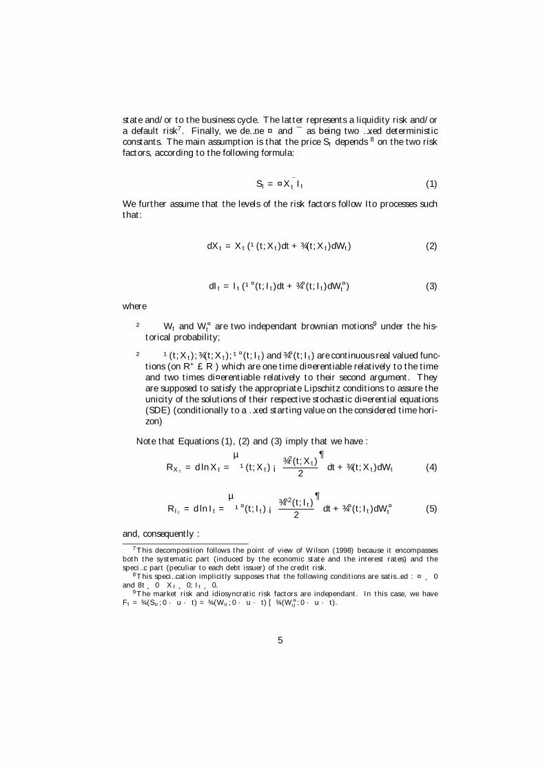
state and/or to the business cycle. The latter represents a liquidity risk and/ora default risk7. Finally, we de…ne ¤ and ¯ as being two …xed deterministicconstants. The main assumption is that the price St depends 8 on the two riskfactors, according to the following formula:

St = ¤X¯t It (1)

We further assume that the levels of the risk factors follow Ito processes suchthat:

dXt = Xt (¹(t; Xt)dt + ¾(t; Xt)dWt) (2)

dIt = It (¹¤(t; It)dt + ¾¤(t; It)dW ¤t ) (3)

where

² Wt and W ¤t are two independant brownian motions9 under the his-

torical probability;

² ¹(t; Xt); ¾(t; Xt); ¹¤(t; It) and ¾¤(t; It) are continuous real valued func-tions (on R+ £ R ) which are one time di¤erentiable relatively to the timeand two times di¤erentiable relatively to their second argument. Theyare supposed to satisfy the appropriate Lipschitz conditions to assure theunicity of the solutions of their respective stochastic di¤erential equations(SDE) (conditionally to a …xed starting value on the considered time hori-zon)

Note that Equations (1), (2) and (3) imply that we have :

RXt = d ln Xt =

µ¹(t; Xt) ¡ ¾2(t; Xt)

2

¶dt + ¾(t; Xt)dWt (4)

RIt = d ln It =

µ¹¤(t; It) ¡ ¾¤2(t; It)

2

¶dt + ¾¤(t; It)dW ¤

t (5)

and, consequently :

7 This decomposition follows the point of view of Wilson (1998) because it encompassesboth the systematic part (induced by the economic state and the interest rates) and thespeci…c part (peculiar to each debt issuer) of the credit risk.

8 This speci…cation implicitly supposes that the following conditions are satis…ed : ¤ ¸ 0and 8t ¸ 0 Xt ¸ 0; It ¸ 0.

9 The market risk and idiosyncratic risk factors are independant. In this case, we haveFt = ¾ (Su; 0 · u · t) = ¾ (Wu; 0 · u · t) [ ¾ (W ¤

u ; 0 · u · t).

5

RSt= ¯ RXt

+ RIt

where RSt , RXt and RIt are the returns on the contingent claims whose value areSt; Xt and It. According to Sharpe, RIt is the sum of the risk-free rate of interestRft and of a random variable whose expected value is zero (RIt = Rft +½It

withE

£½It

jFt

¤= 0). Finally, equations (4) and (5) are coherent with Sharpe’s view

if we identify³

¹¤(t; It) ¡ ¾¤2(t;It)2

´to (1 ¡ ¯) Rft. We now study the in‡uence

of the assumptions above-mentioned on the stock’s dynamic and then on thevaluation of a call written on this stock.

Dynamic of the price of the underlying asset :

We apply Ito’s lemma to the underlying asset’s price considered as a two-variables function St = S(Xt; It). Indeed, St depends exclusively on the levelsof the market and of the speci…c risks10 :

dSt =@S

@XdXt +

@S

@IdIt +

1

2

µ@2S

@X2¾2(t; St)X

2t +

@2S

@I2¾¤2(t; It)I

2t

¶dt

We replace dXt and dIt with their respective expressions and we compute thepartial derivatives of price of the stock with respect to the risk factors :

@S@X = ¯¤Xt

¯¡1It = ¯ St

Xt

@S@I = ¤X¯

t = St

It

@2S@X2 = ¯ (¯ ¡ 1) ¤X¯¡2

t It = ¯ (¯ ¡ 1) St

Xt2

@2S@I2 = 0

which leads to the following relation :

dSt

St= ¨(t; Xt; It)dt + ª(t; Xt; It)d!t

with

¨(t; Xt; It) = ¯¹(t; Xt) + ¹¤(t; It) +1

2¯ (¯ ¡ 1) ¾2(t; Xt)

ª(t; Xt; It) =

q¯2¾2(t; Xt) + ¾¤2(t; It)

d!t =¯¾(t; Xt)dWt + ¾¤(t; It)dW ¤

tq¯2¾2(t; Xt) + ¾¤2(t; It)

: standard brownian motion

10 S is a continuous and twice di¤erentiable function with respect to each argument X andI.

6

We obtain the stock’s dynamic expressed in terms of the parameters charac-terizing the evolution of the risk factors encompassed in its price. Note that theexistence of this SDE’s solution results from the continuity of the parameterscharacterizing the di¤usions of the two risk factors. The uniqueness results fromthe Lipschitz conditions which have been assumed to hold.

Dynamic of the call’s price :

We now consider a european call written on the stock, namely the underlyingasset, with a strike price K and a maturity date T . The value C of the europeancall depends on the levels of the two risk factors and on time; it can be speci…edas follows :

C = C(t; Xt; It)

which allows us to apply the multivariate Ito’s lemma to the call’s price 11. Wethen obtain the following equation :

dC =

·CX¹(t; Xt)Xt + CI¹¤(t; It)It + Ct

+12

¡CXX¾2(t; Xt)X

2t + CII¾¤2(t; It)I

2t

¢ ¸dt

+ [CX¾(t; Xt)XtdWt + CI¾¤(t; It)ItdW ¤t ]

under the limit condition :

C(T; XT ; IT ) = (ST ¡ K)+ = Max (0; ST ¡ K)

As usual, we …rst consider a self-…nancing strategy allowing the replication ofthe call with the two risk factors. The value Vt of the replicating portfolio, isde…ned by

Vt = ¢tIt + ¡tXt = C(t; Xt; It)

which gives ¢t = CI and ¡t = CX :

11 We use the following standard denominations::

@C@t

= Ct@2C

@X@I= @2C

@I@X= CXI = CIX

@C@X

= CX@2C@X2 = CXX

@C@I

= CI@2C@I2 = CII

CZ =

·CX

CI

¸CZZ =

·CXX CXI

CIX CII

¸

7

Then, we build a hedging portfolio, using the replicating portfolio and thecall itself12. The hedging portfolio is immune against the market risk and theidiosyncratic risk, and its value ¼t may be expressed as :

¼t = Vt ¡ C(t; Xt; It) = CIIt + CXXt ¡ C(t; Xt; It)

If there is no arbitrage opportunity, the return of the immune portfolio is equalto the risk free rate of return13; hence:

d¼t = r¼tdt

CIdIt + CXdXt ¡ dC = r (CIIt + CXXt ¡ C(t; Xt; It)) dt

Replacing the stochastic di¤erentials with their respective expressions and group-ing the stochastic and the deterministic terms, we get the following partial dif-ferential equation (PDE) :

rCXXt +1

2CXX¾2(t; Xt)X

2t + Ct ¡ rC +

1

2CII¾¤2(t; It)I

2t + rCIIt = 0

We now assume that the level of each risk factor follows a geometric brownianmotion with constant drift and volatility14, that is to say :

¹(t; Xt) = ¹ ¾(t; Xt) = ¾

¹¤(t; It) = ¹¤ ¾¤(t; It) = ¾¤

where ¹; ¾; ¹¤ and ¾¤ are deterministic constants. We therefore assume a con-stant risk-free rate of interest ( ¹¤ ¡(¾¤2=2) = Rf .). The PDE above-mentionedtakes the form :·

rCXXt +1

2CXX¾2X2

t + Ct ¡ rC

¸+

·1

2CII¾¤2I2

t + rCIIt

¸= 0

PDE resolution :

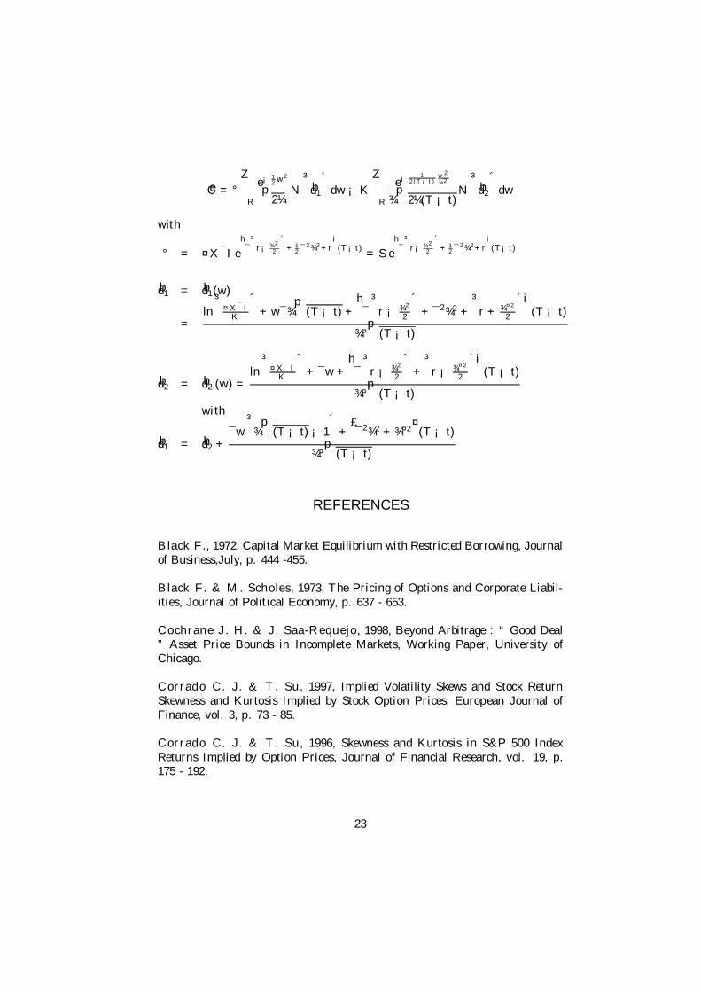
We show in the appendix that the PDE resolution leads to the followingformulation for the price of the two risk factors european call :

C(T ¡ t; Xt; It; K; r; ¾; ¾¤) (6)

= °t

ZR

e¡ 12 w2

p2¼

N³ bd1 (w)

´dw ¡ Ke¡r(T¡t)

ZR

e¡ 12(T ¡t)

w2

¾2

¾p

2¼(T ¡ t)N

³ bd2 (w)´

dw

12 The hedging portfolio corresponds to the selling of one unit of call and to the simultaneousbuying of ¢t units of speci…c risk factor and of ¡t units of market factor.

13 This interest rate is temporarily supposed constant.14 This is equivalent to suppose that each factor’s rate of return follows a normal distribution

law.

8

with

°t = ¤X¯t It e

h¯

³r¡ ¾2

2

´+ 1

2 ¯2¾2i(T¡t)

= St e

h¯

³r¡ ¾2

2

´+ 1

2 ¯2¾2i

(T ¡t)

bd1(w) =

ln³

¤X¯t It

K

´+ w¯¾

p(T ¡ t) +

24 ¯³

r ¡ ¾2

2

´+ ¯2¾2

+³

r + ¾¤2

2

´ 35 (T ¡ t)

¾¤p(T ¡ t)

bd2 (w) =ln

³¤X¯

t It

K

´+ ¯w +

h¯

³r ¡ ¾2

2

´+

³r ¡ ¾¤2

2

´i(T ¡ t)

¾¤p(T ¡ t)

For further details about the computation of the analytical formula asso-ciated to the pricing of the european call, the reader is invited to consult theappendix. Note that the case ¯ = 0 corresponds to the formula of Black &Scholes with St = ¤It. Moreover recalling that ª =

p¾¤2 + ¾2¯2, the formula

above-mentioned has the new expression :

C(T ¡ t; St; K; r; ª; ¾) (7)

= °t

ZR

e¡ 12 w2

p2¼

N³ bd1 (w)

´dw ¡ Ke¡r(T¡t)

ZR

e¡ 12(T ¡t)

w2

¾2

¾p

2¼(T ¡ t)N

³ bd2 (w)´

dw

with

°t = St e

h¯

³r¡ ¾2

2

´+ 1

2 ¯2¾2i(T¡t)

= ° (St; K; r; (T ¡ t); ª; ¾; ¯)

bd1(w) =ln

¡St

K

¢+ w¯¾

p(T ¡ t) +

h¯

³r ¡ ¾2

2

´+ ¯2¾2

2 +³

r + ª2

2

´i(T ¡ t)q

(T ¡ t)¡ª2 ¡ ¯2¾2

¢bd2 (w) =

ln¡

St

K

¢+ ¯w +

h¯

³r ¡ ¾2

2

´+ ¯2¾2

2 +³

r ¡ ª2

2

´i(T ¡ t)q

(T ¡ t)¡ª2 ¡ ¯2¾2

¢We then notice that the option’s price depends both on the market factor

and the price of the traded asset. The valuation remains therefore possible whenthe speci…c factors become unobservable. Indeed, we no more need to know thevolatilities ¾ and ¾¤ of the market and idiosyncratic factors respectively but onlythe volatilities ¾ and ª of the market factor and the underlying respectively.

3 Diversi…cation or indirect observation of themarket factor

To solve the problem posed by the unobservability of the risk factors–whichis the case in practice–, we adapt the Capital Asset Pricing Model (CAPM) to

9

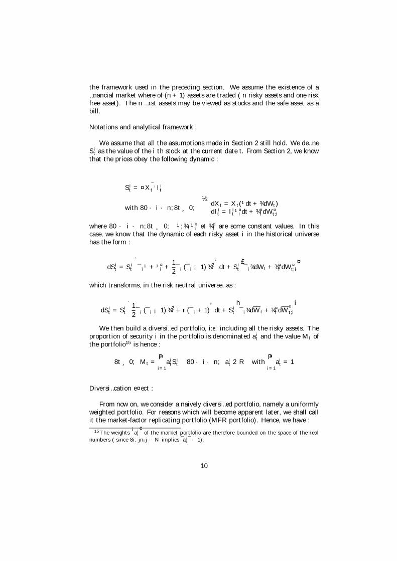
the framework used in the preceding section. We assume the existence of a…nancial market where of (n + 1) assets are traded ( n risky assets and one riskfree asset). The n …rst assets may be viewed as stocks and the safe asset as abill.

Notations and analytical framework :

We assume that all the assumptions made in Section 2 still hold. We de…neSi

t as the value of the i th stock at the current date t. From Section 2, we knowthat the prices obey the following dynamic :

Sit = ¤X

¯it Ii

t

with 80 · i · n; 8t ¸ 0;

½dXt = Xt(¹dt + ¾dWt)dIi

t = Iit¹¤

i dt + ¾¤i dW ¤

t;i

where 80 · i · n; 8t ¸ 0; ¹; ¾; ¹¤i et ¾¤

i are some constant values. In thiscase, we know that the dynamic of each risky asset i in the historical universehas the form :

dSit = Si

t

·¯i¹ + ¹¤

i +1

2¯i (¯i ¡ 1) ¾2

¸dt + Si

t

£¯i¾dWt + ¾¤

i dW ¤t;i

¤which transforms, in the risk neutral universe, as :

dSit = Si

t

·1

2¯i (¯i ¡ 1) ¾2 + r (¯i + 1)

¸dt + Si

t

h¯i¾dW t + ¾¤

i dW¤t;i

iWe then build a diversi…ed portfolio, i:e. including all the risky assets. The

proportion of security i in the portfolio is denominated ait and the value Mt of

the portfolio15 is hence :

8t ¸ 0; Mt =nP

i=1ai

tSit 80 · i · n; ai

t 2 R withnP

i=1ai

t = 1

Diversi…cation e¤ect :

From now on, we consider a naively diversi…ed portfolio, namely a uniformlyweighted portfolio. For reasons which will become apparent later, we shall callit the market-factor replicating portfolio (MFR portfolio). Hence, we have :

15 The weights¡ai

t

¢of the market portfolio are therefore bounded on the space of the real

numbers ( since 8i; jnij · N implies¯̄ai

t

¯̄ · 1).

10

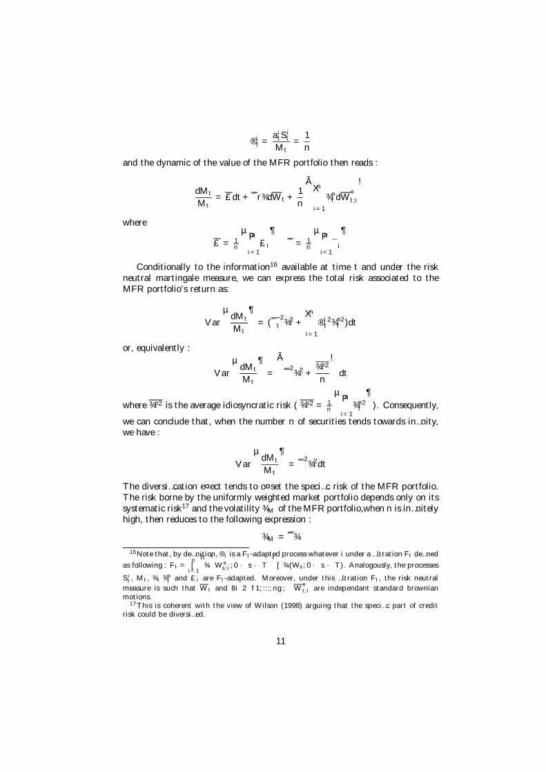
®it =

aitS

it

Mt=

1

n

and the dynamic of the value of the MFR portfolio then reads :

dMt

Mt= £dt + ¯r¾dW t +

1

n

ÃnX

i=1

¾¤i dW

¤t;i

!where

£ = 1n

µnP

i=1£i

¶¯ = 1

n

µnP

i=1¯i

¶Conditionally to the information16 available at time t and under the risk

neutral martingale measure, we can express the total risk associated to theMFR portfolio’s return as:

V ar

µdMt

Mt

¶= (¯t

2¾2 +

nXi=1

®it2¾¤2

i )dt

or, equivalently :

V ar

µdMt

Mt

¶=

ï

2¾2 +

¾¤2

n

!dt

where ¾¤2 is the average idiosyncratic risk ( ¾¤2 = 1n

µnP

i=1¾¤2

i

¶). Consequently,

we can conclude that, when the number n of securities tends towards in…nity,we have :

V ar

µdMt

Mt

¶= ¯

2¾2dt

The diversi…cation e¤ect tends to o¤set the speci…c risk of the MFR portfolio.The risk borne by the uniformly weighted market portfolio depends only on itssystematic risk17 and the volatility ¾M of the MFR portfolio,when n is in…nitelyhigh, then reduces to the following expression :

¾M = ¯¾

16 Note that, by de…nition, ®i is a Ft-adapted process whatever i under a …ltration Ft de…ned

as following : Ft =n[

i=1

h¾

³W ¤

s;i; 0 · s · T´i

[¾ (Ws; 0 · s · T ). Analogously, the processes

Sit , Mt, ¾, ¾¤

i and £i are Ft-adapted. Moreover, under this …ltration Ft, the risk neutralmeasure is such that W t and 8i 2 f1; :::; ng ; W

¤t;i are independant standard brownian

motions.17 This is coherent with the view of Wilson (1998) arguing that the speci…c part of credit

risk could be diversi…ed.

11

Moreover, the price of the european call on stock i now reads, using the samedenominations as before, except that the superscript i is now explicitly takeninto account :

C

µT ¡ t; Si

t ; Ki; r; ªi;¾M

¯; ¯i

¶(8)

= °it

ZR

e¡ 12 w2

p2¼

N³ bd1 (w)

´dw ¡ Kie¡r(T¡t)

ZR

e¡ 12(T ¡t)

w2

¾2

¾p

2¼(T ¡ t)N

³ bd2 (w)´

dw

with

°it = Si

t e

·¯i

µr¡ (¾M =¯)2

2

¶+ 1

2 (¯i¾M

¯)2

¸(T¡t)

bd1(w) =

ln³

Sit

Ki

´+ w( ¯i¾M

¯)p

(T ¡ t) +

24 ¯i

³r ¡ (¾M =¯)2

2

´+

(¯i¾M =¯)2

2 +³

r +ª2

i

2

´ 35 (T ¡ t)

q(T ¡ t)

¡ª2

i ¡ (¯i¾M=¯)2¢

bd2 (w) =

ln³

Sit

Ki

´+ ¯iw +

24 ¯i

³r ¡ (¾M =¯)2

2

´+ (¯i¾M =¯)2

2

+³

r ¡ ª2i

2

´ 35 (T ¡ t)

q(T ¡ t)

¡ª2

i ¡ (¯i¾M=¯)2¢

Finally, on a …nancial market where n risky assets and one risk free asset aretraded in such a way that each risky asset depends on a market factor and anidiosyncratic factor according to equation (6), the factors’ unobservability doesnot preclude the risk neutral valuation of options. One has just to substitutethe ratio

³¾M

¯

´of the volatility of the market portfolio’s return to the average

beta for the volatility ¾ of the market factor. The price of an option may beexpressed in terms of the volatilities of a naively diversi…ed market portfolio andof the underlying asset respectively. Option pricing remains therefore possibleeven if none of the factors is tradable –which is the case in practice–.

4 Comparison with the formulae of Black & Sc-holes and of Corrado & Su

In this section, we compare our option valuation formula to the valuationsproposed by Black & Scholes (1973) and by Corrado & Su (1996, 1997). Giventhe complexity related to the computation of the comparative statics of ouranalytical formula, the comparisons are achieved through simulations.

12

4.1 Black & Scholes

4.1.1 Comparison with a varying beta

In this subsection, we carry out simulations where beta is the only pa-rameter which is varying. Simulations are achieved using the next values ofparameters :

S = K = 100 ¾ = ¾¤ = 1r = 0:10 (T ¡ t) = 0:25

We therefore consider at-the-money calls and, to make the comparison fair, weimpose the next relation:

¾2BS = ¯2 ¾2 + ¾¤2

where ¾BS represents the aggregated volatility of the underlying (i. e. withoutany distinction between speci…c and systematic risks). We then plot the pric-ing di¤erence between the call prices induced from our two factors valuationmethod and those issued from the Black & Scholes’ valuation in terms of thebeta parameter characterizing the underlying, namely the di¤erence betweenthe two factors pricing and the Black & Scholes’ one :

Di¤erence between the two factors pricing and Black & Scholes’ pricing.

We observe that the pricing di¤erence grows when the beta increases, and re-duces when the beta starts decreasing from the level of 0:40. Notice that, asexpected, the pricing error is null for a zero beta since for a null beta our val-uation formula reduces to the Black & Scholes’ formula. Moreover, the pricingdi¤erence is also null when the beta is equal to 0:80.

13

4.1.2 The role of “moneyness”

We now express the prices of calls as functions of the moneyness (i. e. ratioof the underlying’s price to the strike (S=K)) associated to the pricing, given a…xed beta. Simulations are undertaken, using the following values for the otherparameters :

K = 100 ¾ = ¾¤ = 1S = moneyness ¤ Kr = 0:10 (T ¡ t) = 0:25

We still have the following relation :

¾2BS = ¯2 ¾2 + ¾¤2

We successively realize our simulations for some values of the beta18 rangingfrom 0:1 to 1:5. To have a global view, we plot the european call pricing di¤er-ence between our two factors method and the valuation of Black & Scholes infunction of the moneyness and of the beta. The graph under-mentioned illus-trates then the pricing di¤erence between our two factors methodology and thevaluation of Black & Scholes for varying beta and moneyness parameters.

0,10

0,20

0,29

0,39

0,48

0,58

0,68

0,77

0,87

0,96

1,06

1,16

1,25

1,35

1,44

1,54

1,64

1,73

1,83

1,92

0,1 0,75

1,1

-2,00

0,00

2,00

4,00

6,00

8,00

10,00

12,00

14,00

Pric

ing

diffe

renc

e

Moneyness

Beta

Di¤erence between the european call prices.

Note that for beta values inferior to 0:8, the pricing di¤erence is negative (i.e. : the pricing of Black & Scholes overestimates the european call price) whilein the opposite case, this di¤erence is positive (i. e. : the pricing of Black &

18 The case ¯ = 0 is uninteresting because our two factors pricing formula reduces to thevaluation formula of Black & Scholes, which gives a nul pricing error whatever the value ofthe moneyness.

14

Scholes underestimates the european call price). This di¤erence being almostnull when the beta equals 0:8. Moreover, the more the moneyness is high, themore important is the pricing di¤erence in absolute value.

4.1.3 Existence of a volatility smile

We consider here that call prices induced from our two factors formula (i.e. : the pricing of Chauveau & Gatfaoui) correspond to the prices observed onthe market. We assume the following values of parameters :

K = 100 ¾ = ¾¤ = 0:16S = moneyness ¤ K ¯ = 0:5r = 0:10 (T ¡ t) = 0:25

Starting from the call prices above-mentioned, we invert the Black & Scholes’formula to deduce the associated values of the implied volatility, which allowsto plot the graph corresponding to the implied volatility’s evolution in functionof the moneyness.

0,15

0,25

0,35

0,45

0,55

0,65

0,75

0,85

0,40

0,44

0,47

0,51

0,55

0,58

0,62

0,65

0,69

0,73

0,76

0,80

0,84

0,87

0,91

0,95

0,98

1,02

1,05

1,09

1,13

1,16

1,20

1,24

1,27

1,31

1,35

1,38

1,42

1,45

1,49

1,53

1,56

1,60

Moneyness

Vola

tility

We then …nd again the volatility smile describing the well known bias of theBlack & Scholes’ formula generated by the constant volatility hypothesis. Be-sides, this bias is the object of a correction method recently proposed and whichis presented in the next section.

4.2 Corrado & Su

In this section, we compare our pricing formula with the ones of Corrado& Su and of Black & Scholes respectively in order to realize some comparisonsbetween those three valuation methods.

15

4.2.1 Pricing formula

In 1996, Corrado & Su developped a methodology to correct the bias de-scribed by the volatility smile in the Black & Sholes’ formula. They used aGram-Charlier series expansion of the standard normal density function, whichlead them to establish the following european call valuation formula :

CCS(t; S) = CBS (t; S) + ¹3Q3 + (¹4 ¡ 3) Q4

with

CBS (t; S) : the Black & Scholes’ formula by replacing ¾BS with ¾CS;

d1 =ln( St

K )+

µr+

¾2CS2

¶(T¡t)

¾CS

p(T¡t)

;

Q3 = 16 S ¾CS

p(T ¡ t)

h³2¾CS

p(T ¡ t)

´n (d1) ¡ ¾2

CS (T ¡ t) N (d1)i;

Q4 = 124 S ¾CS

p(T ¡ t)

" nd2

1 ¡ 1 ¡ 3¾CS

p(T ¡ t)

³d1 ¡ ¾CS

p(T ¡ t)

´on (d1) + ¾3

CS (T ¡ t)3=2 N (d1)

#;

n (:) : the standard normal density function;

N (:) : the cumulative distribution function associated to the standard normallaw;

¾CS; ¹3; ¹4 : parameters of volatility, skewness and kurtosis respectively asso-ciated to the underlying’s dynamic.

4.2.2 Comparison relatively to the moneyness

To compare our two factors pricing formula with that of Corrado & Su,we use the parameters’ values presented in the previous section to generatecall prices according to the pricing of Chauveau & Gatfaoui. Always assumingthat the prices then induced are the observed market prices, we estimate theparameters ¾CS, ¹3 and ¹4 of the Corrado & Su’s formula when consideringthe call prices previously computed. The estimation is achieved by numericallysolving the following problem :

Min¾CS ;¹3 ;¹4

8<:Xj

[C (t; moneynessj) ¡ CCS (t; moneynessj)]2

9=;where moneynessj = St

Kjwith Kj 2 f65; ::; 135g. The minimization of the sum

of the squared pricing errors is carried out through a quasi-Newton method

16

using the algorithm of Davidon-Fletcher-Powell19, which allows to obtain thefollowing values of parameters : ¾CS = 0:29947828, ¹3 = ¡1:7423441 and¹4 = 8:883017220. Introducing those estimations into the formula of Corrado &Su allows then to compute the call prices associated giving the graph underneathin which the call prices induced from the method of Chauveau & Gatfaoui, theformula of Corrado & Su and the valuation of Black & Scholes are respectivelydrawn in blue, black and red.

European call pricing according to the three formulae presented.

Considering the graph and omitting the negative pricing problem presented bythe formula of Corrado & Su for small values of the moneyness, we observe thatthe formula of Corrado & Su seems to lie between our two factors valuationformula and the Black & Scholes’ formula.

5 Conclusion

In this paper, we have proposed an analytical formula for valuing a europeancall with two risk factors : the …rst factor corresponds to the systematic riskand the second factor corresponds to the speci…c risk of the underlying asset,as in Sharpe’s simpli…ed model21. We derived our valuation formula from arisk disaggregation in the Black & Scholes’ pricing formula, which allowed usto get an analytical expression for the european call pricing. The parameters

19 For further explanation, the reader is invited to consult the book of Press, Flannery,Teukolsky & Vetterling (1989).

20 Note that those values show that, on one hand, the distribution of the call prices is left-skewed, and on the other hand, this distribution is described by an excess of kurtosis relativelyto a normal law, which indicates the existence of a left fat tail in the distribution.

21 This decomposition could also be improved if we consider that systematic risk and speci…crisk are themselves some aggregation of respectively two di¤erent series of in‡uent variables(i. e. : multifactor framework)

17

of this formula therefore depend on the volatilities of the two risk factors, or,alternatively, on the volatility of the market factor and on that of the stock.

We then built a market factor replicating portfolio which is a naively divesi-…ed portfolio and we studied the modi…cations induced in the CAPM framework.We found that, under some regularity conditions, the diversi…cation e¤ect knownto o¤set the speci…c risk applies. The price of a european call on a stock maythen be expressed in terms of the volatilities of the MFR portfolio and of theunderlying stock (and of its beta).

Finally, we made a few simulations in order to compare our analytical for-mula with those of Black & Scholes and of Corrado & Su. First, the comparisonwith the formula of Black & Scholes underlines the fact that the distinction be-tween the systematic risk and the idiosyncratic risk brings an additional degreeof accuracy in the european call valuation. Moreover, assuming that the euro-pean call prices induced from our two factors formula are correct and obtainingthe implicit volatility by inverting the Black & Scholes’ formula, leads to the ev-idence of a volatility smile. Second, the comparison with the valuation methodproposed by Corrado & Su shows that european call prices induced from thepricing of Chauveau & Gatfaoui exhibit skewness and kurtosis characteristics inaccordance with the observed market behavior. Furthermore, the results gen-erated by simulations seem to suggest that the formula of Corrado & Su liesbetween our two factors valuation formula and the pricing formula of Black &Scholes.

The results in this paper are to be completed by a test on empirical data.This is all the more essential that we have imposed a volatility constraint whencomparing our formula with that of Black & Scholes.

6 Appendix : The call pricing with two risk fac-tors

We introduce here the pricing framework of the call, which is the followingone : Analogous to the no arbitrage opportunity principle, we have the nextrelation under the risk neutral measure Q associated to the valuation of the

bidimensional process Zt =

·Xt

It

¸:

8t 2 [0; T ] ;

C(t; Xt; It) = C(t; Zt) = EQ

he¡r(T¡t)C(T; ZT )ÁFt

i= e¡r(T ¡t)EQ [C(T; ZT )ÁZt]

which can be written :

18

C(t; Z) = e¡r(T¡t)

ZR£R

8><>:³n

¤¡a0 ¢ eYT

¢¯ ¡b0 ¢ eYT

¢o¡ K

´+

f (YT ÁYt)

9>=>; dYT;1dYT;2

(9)

where

a =

·10

¸b =

·01

¸8W =

·W1

W2

¸2 R2; eT =

·eW1

eW2

¸and f (YT ÁYt) represents the conditional density of YT given Yt. We know thatthe law of YT given Yt corresponds to a bidimensional normal law N (MOYt; V ARt)in a risk neutral universe such that :

MOYt = Yt + (T ¡ t)Ht =

·Y 1

t

Y 2t

¸+ (T ¡ t)

"r ¡ ¾2

2

r ¡ ¾¤2

2

#

§t = §(t; Xt; It) =

·Xt¾(t; Xt) 0

0 It¾¤(t; It)

¸

V ARt = §(t; Xt; It)§0(t; Xt; It) (T ¡ t) = (T ¡ t) §t§

0t

Knowing the law of YT given Yt , we can compute the integral of the relation(9) after introducing the following notations :

g(ZT ) = g(eYT ) =³n

¤¡a0 ¢ eYT

¢¯ ¡b0 ¢ eYT

¢o¡ K

´+

= 1= h(eYT )

with

1= = indicator function of the set == =

nh¤

¡a0 ¢ eYT

¢¯ ¡b0 ¢ eYT

¢i¡ K ¸ 0

oh(eYT ) =

³¤

¡a0 ¢ eYT

¢¯ ¡b0 ¢ eYT

¢´¡ K

The relation (6) is written :

C(t; Xt; It) = e¡r(T¡t)

ZR2

1=©

h(eYT )f (YT ÁYt)ª

dYT;1dYT;2 (10)

19

Or

C(t; Xt; It) = e¡r(T¡t)

Z=

©h(eYT )f (YT ÁYt)

ªdYT;1dYT;2 (11)

We now explain how to calculate the call price with two risk factorswhen achieving the following integration22 :

eC =C(t; Z)

e¡r(T¡t)=

Zu2R2;=

(h(eu+MOY ) 1

2¼(T¡t)¾¾¤

exph¡ 1

2(T¡t)

³u2

1

¾2 +u2

2

¾¤2

´i )du1du2

eC =

Zu2R2;=

8<:n³

¤¡a0 ¢ eu+MOY

¢¯ ¡b0 ¢ eu+MOY

¢´¡ K

o1

2¼(T¡t)¾¾¤ exph¡ 1

2(T¡t)

³u2

1

¾2 + u22

¾¤2

´i 9=; du1du2

eC =

Zu2R2;=

8<:³

¤¡a0 ¢ eu+MOY

¢¯ ¡b0 ¢ eu+MOY

¢´1

2¼(T¡t)¾¾¤ exph¡ 1

2(T¡t)

³u2

1

¾2 +u2

2

¾¤2

´i 9=; du1du2

¡K

Zu2R2;=

½1

2¼(T ¡ t)¾¾¤ exp

·¡ 1

2(T ¡ t)

µu2

1

¾2+

u22

¾¤2

¶¸¾du1du2

We pose eC = eC1 + eC2 with :

eC1 =

Zu2R2;=

8<:³

¤¡a0 ¢ eu+MOY

¢¯ ¡b0 ¢ eu+MOY

¢´1

2¼(T ¡t)¾¾¤ exph¡ 1

2(T¡t)

³u2

1

¾2 +u2

2

¾¤2

´i 9=; du1du2

eC2 = ¡K

Zu2R2;=

½1

2¼(T ¡ t)¾¾¤ exp

·¡ 1

2(T ¡ t)

µu2

1

¾2+

u22

¾¤2

¶¸¾du1du2

UT ÁU v N (0; V AR)

= =nh

¤¡a0 ¢ eu1+MOY1

¢¯ ¡b0 ¢ eu2+MOY2

¢i¡ K ¸ 0

o=

½¯ (u1 + MOY1) + (u2 + MOY2) ¸ ln

µK

¤

¶¾22 To simplify the proof, we forget the time indexation at the current date.

20

First member integration :

eC1 = ®

Zu2R2;=

½e¯u1eu2

2¼(T ¡ t)¾¾¤ exp

·¡ 1

2(T ¡ t)

µu2

1

¾2+

u22

¾¤2

¶¸¾du1du2

with

® = ¤X¯Ie

h¯

³r¡ ¾2

2

´+

³r¡ ¾¤2

2

´i(T¡t)

Applying the Fubini theorem, we can write the following relation about the …rstmember :

eC1 = ®

ZR

e¯u1e¡ 12(T ¡t)

u21

¾2p2¼(T ¡ t)¾

J1(u1)du1

with

J1(u1) =

Z +1

d

eu2p2¼(T ¡ t)¾¤ e¡ 1

2(T ¡t)

u22

¾¤2 du2

d = ln

µK

¤X¯I

¶¡ ¯u1 ¡

·¯

µr ¡ ¾2

2

¶+

µr ¡ ¾¤2

2

¶¸(T ¡ t)

An appropriate change of variable allows us to establish the following result :

J1(u1) = e12 ¾¤2(T¡t)N

³ bd´with

bd = bd(u1) =ln

³¤X¯I

K

´+ ¯u1 +

h¯

³r ¡ ¾2

2

´+

³r + ¾¤2

2

´i(T ¡ t)

¾¤p(T ¡ t)

and N(:) the standard normal cumulative distribution function.

A second change of variable under the integral concerning u1 allows then topose :

eC1 = °

ZR

e¡ 12 w2

p2¼

N³ bd1

´dw

21

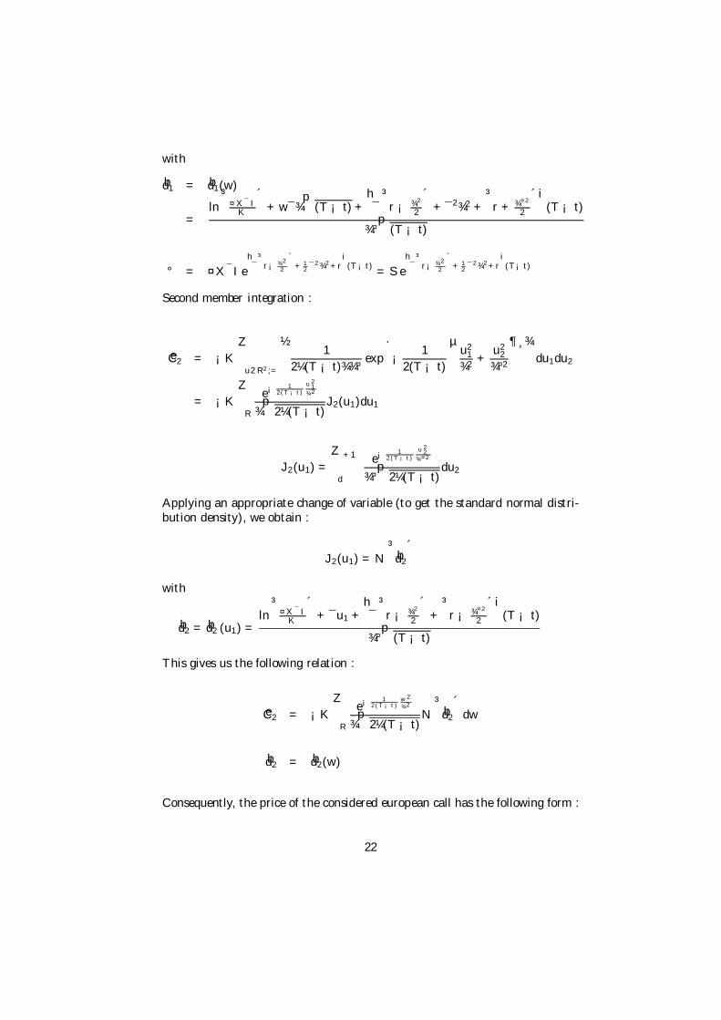
with

bd1 = bd1(w)

=ln

³¤X¯I

K

´+ w¯¾

p(T ¡ t) +

h¯

³r ¡ ¾2

2

´+ ¯2¾2 +

³r + ¾¤2

2

´i(T ¡ t)

¾¤p(T ¡ t)

° = ¤X¯I e

h¯

³r¡ ¾2

2

´+ 1

2 ¯2¾2+ri

(T ¡t)= S e

h¯

³r¡ ¾2

2

´+ 1

2 ¯2¾2+ri(T¡t)

Second member integration :

eC2 = ¡K

Zu2R2;=

½1

2¼(T ¡ t)¾¾¤ exp

·¡ 1

2(T ¡ t)

µu2

1

¾2+

u22

¾¤2

¶¸¾du1du2

= ¡K

ZR

e¡ 12(T ¡t)

u21

¾2

¾p

2¼(T ¡ t)J2(u1)du1

J2(u1) =

Z +1

d

e¡ 12(T ¡t)

u22

¾¤2

¾¤p2¼(T ¡ t)

du2

Applying an appropriate change of variable (to get the standard normal distri-bution density), we obtain :

J2(u1) = N³ bd2

´with

bd2 = bd2 (u1) =ln

³¤X¯I

K

´+ ¯u1 +

h¯

³r ¡ ¾2

2

´+

³r ¡ ¾¤2

2

´i(T ¡ t)

¾¤p(T ¡ t)

This gives us the following relation :

eC2 = ¡K

ZR

e¡ 12(T ¡t)

w2

¾2

¾p

2¼(T ¡ t)N

³ bd2

´dw

bd2 = bd2(w)

Consequently, the price of the considered european call has the following form :

22

eC = °

ZR

e¡ 12 w2

p2¼

N³ bd1

´dw ¡ K

ZR

e¡ 12(T ¡t)

w2

¾2

¾p

2¼(T ¡ t)N

³ bd2

´dw

with

° = ¤X¯I e

h¯

³r¡ ¾2

2

´+ 1

2 ¯2¾2+ri

(T ¡t)= S e

h¯

³r¡ ¾2

2

´+ 1

2 ¯2¾2+ri(T¡t)

bd1 = bd1(w)

=ln

³¤X¯I

K

´+ w¯¾

p(T ¡ t) +

h¯

³r ¡ ¾2

2

´+ ¯2¾2 +

³r + ¾¤2

2

´i(T ¡ t)

¾¤p(T ¡ t)

bd2 = bd2 (w) =ln

³¤X¯I

K

´+ ¯w +

h¯

³r ¡ ¾2

2

´+

³r ¡ ¾¤2

2

´i(T ¡ t)

¾¤p(T ¡ t)

with

bd1 = bd2 +¯w

³¾

p(T ¡ t) ¡ 1

´+

£¯2¾2 + ¾¤2

¤(T ¡ t)

¾¤p(T ¡ t)

REFERENCES

Black F., 1972, Capital Market Equilibrium with Restricted Borrowing, Journalof Business,July, p. 444 -455.

Black F. & M. Scholes, 1973, The Pricing of Options and Corporate Liabil-ities, Journal of Political Economy, p. 637 - 653.

Cochrane J. H. & J. Saa-Requejo, 1998, Beyond Arbitrage : “ Good Deal” Asset Price Bounds in Incomplete Markets, Working Paper, University ofChicago.

Corrado C. J. & T. Su, 1997, Implied Volatility Skews and Stock ReturnSkewness and Kurtosis Implied by Stock Option Prices, European Journal ofFinance, vol. 3, p. 73 - 85.

Corrado C. J. & T. Su, 1996, Skewness and Kurtosis in S&P 500 IndexReturns Implied by Option Prices, Journal of Financial Research, vol. 19, p.175 - 192.

23

Cox J. C., Ross S. A. & M. Rubinstein, 1979, Option Pricing : A Simpli…edApproach, Journal of Financial Economics, vol. 7.

Daves P. R., Ehrhardt M. C. & R. A. Kankel, 2000, Estimating System-atic Risk : The Choice of Return Interval and Estimation Period, Journal ofFinancial and Strategic Decisions, vol. 13, p. 15 - 34.

Heston S., 1993, A Closed Form Solution for Options with Stochastic Volatilitywith Applications to Bonds and Currency Options, Review of Financial Studies,6, p. 327 - 344.

Lintner J., 1965, Valuation of Risk Assets and The Selection of Risky In-vestments in Stock Portfolios and Capital Budgets, Review of Economics andStatistics, p. 13 - 37.

Lintner J., 1969, The Aggregation of Investor’s Diverse Judgments and Prefer-ences in Purely Competitive Security Markets, Journal of Financial and Quan-titative Analysis, December, p. 347 - 400.

Lucas A., Klaassen P., Spreij P. & S. Straetmans, 2001, Tail Behavior ofCredit Loss Distributions for General Latent Factor Models, Tinbergen InstituteWorking Paper.

Malkiel B. G. & Y. Xu, 2001, Idiosyncratic Risk and Security Returns,Department of Economics, Princeton University Working Paper.

Merton R. C., 1973, An Intertemporal Capital Asset Pricing Model, Econo-metrica, vol. 41, p. 867 - 887.

Mossin J., 1966, Equilibrium in a Capitral Asset Market, Econometrica, Oc-tober, p.768 - 783.

Pham H., 1998, Méthodes d’Evaluation et Couverture en Marché Incomplet,CREST - ENSAE.

Press W. H., Flannery B. P., Teukolsky S. A. & W. T. Vetterling,1989, Numerical Receipes in Pascal, Cambridge University Press.

Quittard-Pinon F., 1993, Marchés des Capitaux et Théorie Financière, Eco-nomica.

Rogers L. C. G. & D. Williams, 1994, Di¤usions, Markov Processes andMartingales : Itô Calculus, Cambridge University Press (Volume 2).

Rogers L. C. G. & D. Williams, 1994, Di¤usions, Markov Processes andMartingales : Foundations, Cambridge University Press (Volume 1).

24

Sharpe W. F., 1970, Portfolio Theory and Capital Markets, Mc Graw-Hill,New-York.

Sharpe W. F., 1963, A Simpli…ed Model For Portfolio Analysis, ManagementScience, vol. 9.

Sharpe W. F., 1964, Capital Asset Prices : A Theory of Market EquilibriumUnder Conditions of Risk, Journal of Finance, vol. 19, p. 425 - 442.

Treynor., 1961, Toward a Theory of the Market Valuue of Risky Assets, Un-published manuscript.

Wilson T. C., 1998, Portfolio Credit Risk, FRBNY Economic Review, p. 71 -82.

** *

25