risk benefit analysis special lectures university of kuwait richard wilson mallinckrodt professor of...
TRANSCRIPT
RISK BENEFIT ANALYSISSpecial Lectures
University of KuwaitRichard Wilson
Mallinckrodt Professor of PhysicsHarvard University
January 13th, 14th and 15th 2002
January 13th 9 am to 2 pm
What do we mean by Risk?Measures of Risk
How do we Calculate Risk?(a) History
(b) Animal analogy(c) Event Tree

Day 2. January 14th 2002Uncertainties and Perception
Types of Uncertainties
Role of Perception.Kahneman’s 2002 economics Nobel prize
We will try to show his effect in classList of interesting attributes
Major differences between Public and Expert perceptions

Day 3 January 15th 2003Formal Risk-benefit comparisons.
Net Present Value Decision Tree
Value of InformationProbability of Causation
Cases:Chernobyl, TMI
BhopalALAR as a pesticide
Research on particulatesSabotage and Terrorism


The Biggest Risk to Life is Birth. Birth always leads to death!
We talk about premature death.

More risk 38 60 55 43 78Less risk 36 13 26 13 6Same amount 24 26 19 40 14Not sure 1 1 0 4 2
Table 1-1. Public Opinion Survey Comparing Risk Today to Risk of Twenty Years Ago
Q: Thinking about the actual amount of risk facing our society, would you say that people are subject to more risk today than they were twenty years ago, less risk today, or about the same amount of risk today as twenty years ago?
Top Coroprate
Executives (N=401)
Investors, Lenders (N=104)
Congress (N=47)
Federal Regulators
(N=47)
Public (N=1,488)
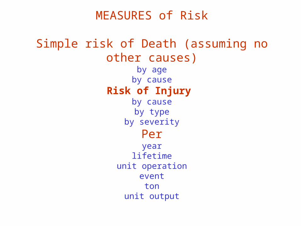
MEASURES of Risk
Simple risk of Death (assuming no other causes)by age
by cause
Risk of Injury by causeby type
by severity
Peryear
lifetimeunit operation
eventton
unit output

RISK MEASURES (continued)
Loss of Life Expectancy (LOLE)Years of Life Lost (YOLL)
Man Days Lost (MDL)Working Days Lost (WDL)
Public Days Lost (PDL)Quality Adjusted Life Years (QALY)
Disability Adjusted Life Years (DALY)
Different decisions may demand different measures
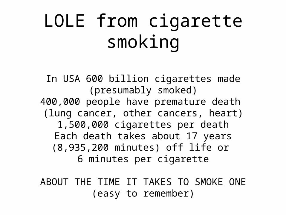
LOLE from cigarette smoking
In USA 600 billion cigarettes made (presumably smoked)400,000 people have premature death
(lung cancer, other cancers, heart)1,500,000 cigarettes per death
Each death takes about 17 years (8,935,200 minutes) off life or
6 minutes per cigarette
ABOUT THE TIME IT TAKES TO SMOKE ONE(easy to remember)

Expectation of Life at Birth in the United States(1900-1928: Death Registration States only)
0
10
20
30
40
50
60
70
80
1900 1910 1920 1930 1940 1950 1960 1970 1980 1990 2000
Year
Exp
ecta
tion
of L
ife a
t Bir
th

Expectation of Life at Birth in the United States(1900-1928: Death Registration States only)
0
10
20
30
40
50
60
70
80
1900 1910 1920 1930 1940 1950 1960 1970 1980 1990 2000
Year
Exp
ecta
tion
of
Lif
e at
Bir
th

WHAT IS LIFE EXPECTANCY?
An artificial construct assuming that the probability of dying as
one ages is the same as the fraction of people dying at the same age at the date of one’s
birth.

Both the specific death rate and the life expectancy at birth have a
dip at 1919world wide influenza epidemic.BUT anyone born in 1919 will
not actually see this dip.Peculiarity of definition of life
expectancy
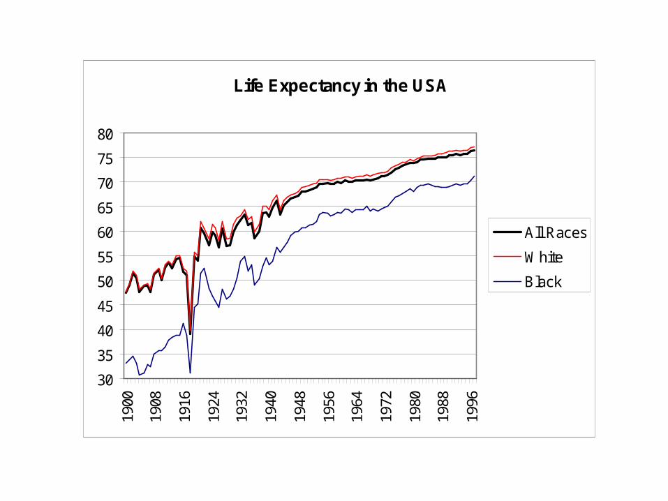
Life Expectancy in the USA
30
35
40
45
50
55
60
65
70
75
8019
00
1908
1916
1924
1932
1940
1948
1956
1964
1972
1980
1988
1996
All Races
White
Black
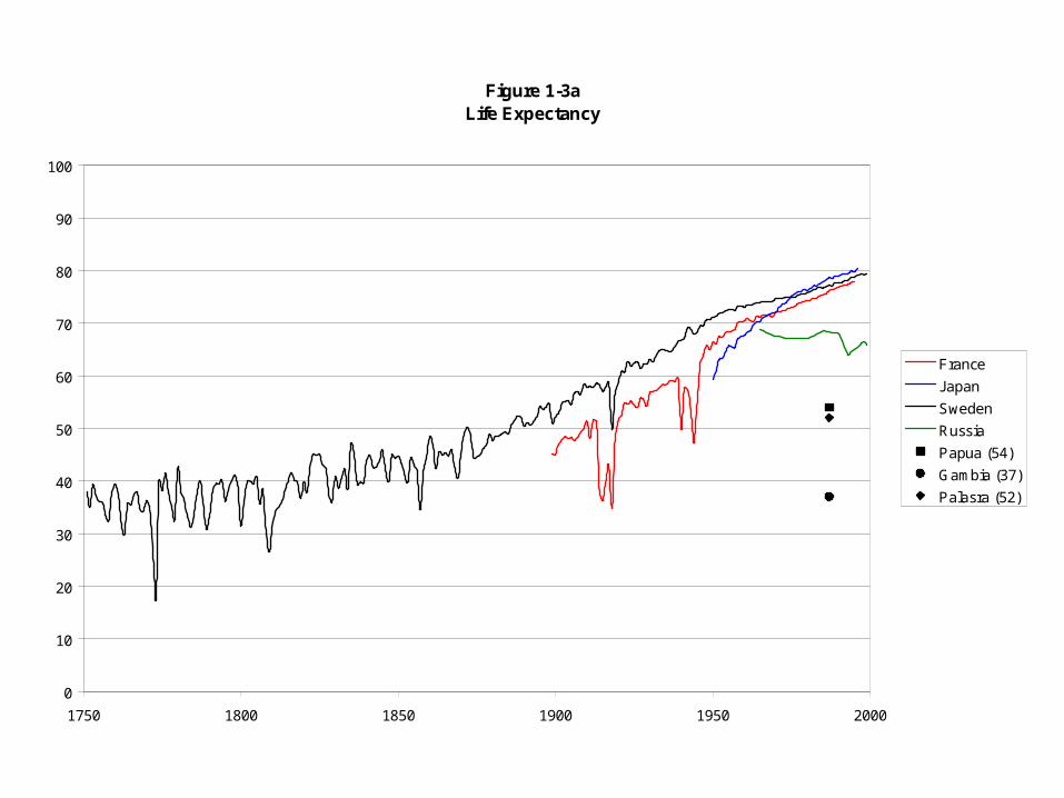
Figure 1-3aLife Expectancy
0
10
20
30
40
50
60
70
80
90
100
1750 1800 1850 1900 1950 2000
France
Japan
Sweden
Russia
Papua (54)
Gambia (37)
Palasra (52)

Half the “Beijing men’ were teenagers.
This puts life expectancy about 15Roman writings imply a life
expectancy of 25.Sweden started life expectancy
statistics early.Russia has been going down
since 1980
Risk is Calculated in Different Ways and that influences perception and decisions.
(1) Historical data(2) Historical data where
Causality is difficult(3) Analogy with Animals
(4) Event tree if no Data exist
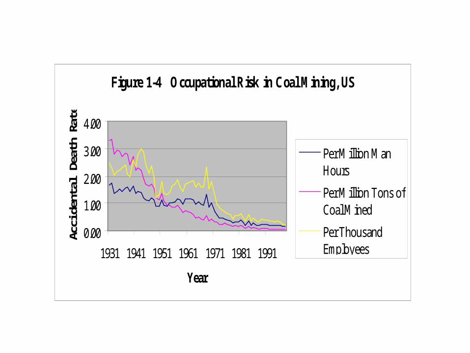
Figure 1-4 Occupational Risk in Coal Mining, US
0.00
1.00
2.00
3.00
4.00
1931 1941 1951 1961 1971 1981 1991
Year
Acci
dent
al D
eath
Rat
e
Per Million ManHours
Per Million Tons ofCoal Mined
Per ThousandEmployees
Risk is different for different measures of risk.
Different decision makers will use different measures depending
on their constituency
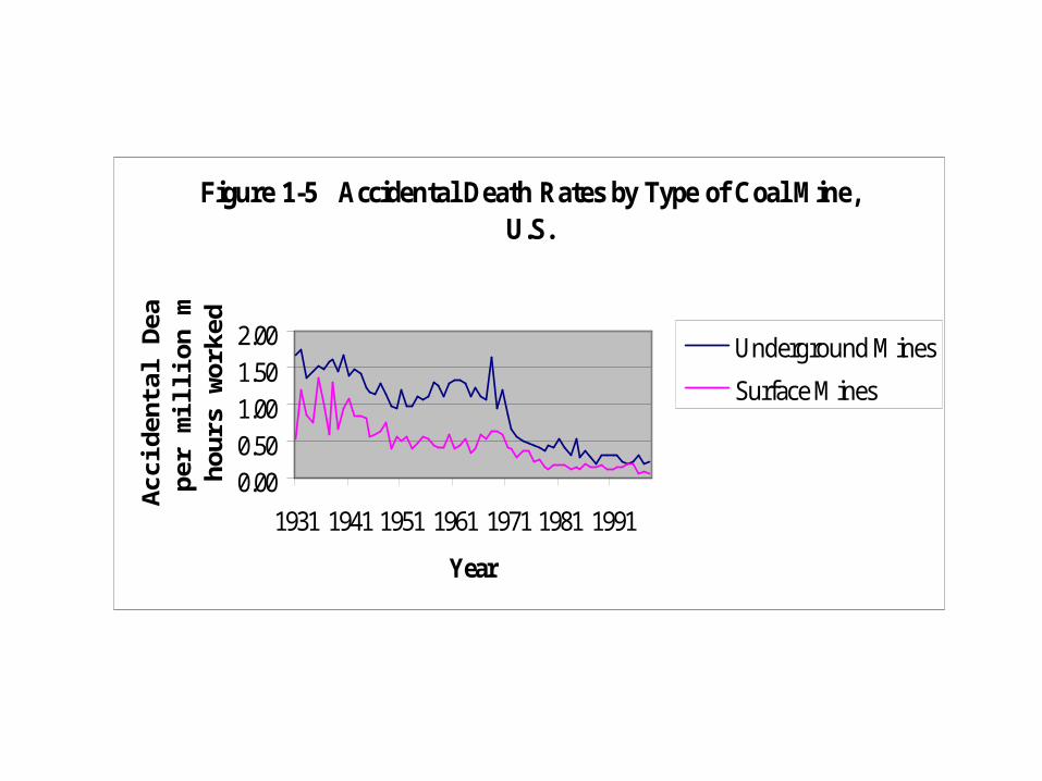
Figure 1-5 Accidental Death Rates by Type of Coal Mine, U.S.
0.00
0.50
1.00
1.50
2.00
1931 1941 1951 1961 1971 1981 1991
Year
Acc
iden
tal D
eath
s pe
r m
illi
on m
an
hour
s w
orke
d Underground Mines
Surface Mines

Figure 2-1 Death Rates for Motor Vehicle Accidents in the United States
0
5
10
15
20
25
30
35
1925 1935 1945 1955 1965 1975 1985 1995
Year
An
nu
al D
eath
Rat
e
per 100,000 population
per 10,000 vehicles
per 1 million vehiclemiles

Accidental Death Rates by Type of Coal Mine, U.S.
0
1
2
3
4
1931 1941 1951 1961 1971 1981 1991
Year
Acc
iden
tal
Dea
ths
per
mil
lion
ton
s of
coa
l pr
odu
ced
Underground Mines
Surface Mines
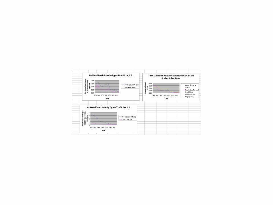
Three Different Metrics of Occupational Risk in Coal Mining, United States
0.00
1.00
2.00
3.00
4.00
1931 1941 1951 1961 1971 1981 1991
Year
Acc
iden
tal D
eath
R
ate
Per M ill ion M anHours
Per Mil lion To ns ofCoal Mined
Per Thous andEmploy ees
Accide ntal De ath Rates by Type of Coal Mine, U.S.
0.00
0.50
1.00
1.50
2.00
1931 1941 1951 1961 1971 1981 1991
Year
Acc
iden
tal D
eath
s pe
r m
illio
n m
an h
ours
w
ork
ed Underg rou nd Mines
Surface Mines
Accide ntal De ath Rates by Type of Coal Mine, U.S.
0
1
2
3
4
1931 1941 1951 1961 1971 1981 1991
Year
Acc
iden
tal
Dea
ths
per
mil
lion
tons
of c
oal
prod
uced Undergroun d Mines
Surface Mines
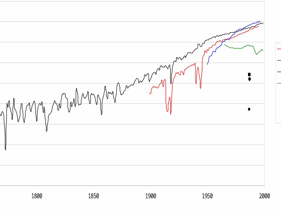
Figure 1-3aLife Expectancy
0
10
20
30
40
50
60
70
80
90
100
1750 1800 1850 1900 1950 2000
France
Japan
Sw eden
Russia
Papua (54)
Gambia (37)
Palasra (52)

Annual Occupation Fatality Rates (US)
0
5
10
15
20
25
30
35
40
45
50
1978
1980
1982
1984
1986
1988
1990
(Year)
Death
s p
er
100,0
00
em
plo
yed
Agriculture, Forestry,Fishing
Mining
Construction
Manufacturing
Private Industry
Transportation andPublic Utilities
Wholesale & RetailTrade
Finance, Insurance,Real Estate
Services
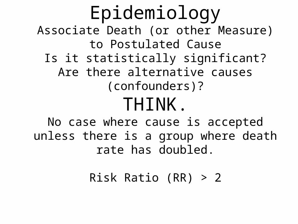
EpidemiologyAssociate Death (or other Measure)
to Postulated CauseIs it statistically significant?
Are there alternative causes (confounders)?
THINK.No case where cause is accepted unless there is a
group where death rate has doubled.
Risk Ratio (RR) > 2
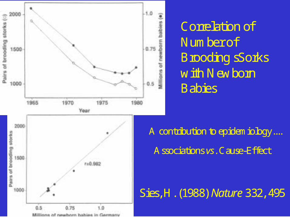
Correlation ofNumber ofBrooding sSorkswith NewbornBabies
Sies, H. (1988) Nature 332, 495
A contribution to epidemiology....
Associations vs. Cause-Effect

Figure 2-7Alternative Dose-Response Models That Fit the Data
Dose
Re
sp
on
se Super Linear
Linear
Hockey Stick
Hormesis
Datum
Datum
Threshold


Annual Death Rate By Daily Alcohol Consumption
0200400600800
1000120014001600
0 0.5 1 2 3 4 5 6
Average Number of Drinks Per Day
Dea
th R
ate
(Per
100
,000
)
Alcohol-augmentedconditionsCardiovasculardiseaseAll causes
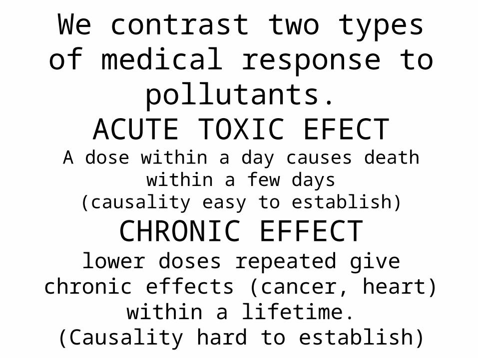
We contrast two types of medical response to pollutants.
ACUTE TOXIC EFECTA dose within a day causes death within a few days
(causality easy to establish)
CHRONIC EFFECTlower doses repeated give chronic effects
(cancer, heart) within a lifetime.(Causality hard to establish)

Characteristics• One dose or dose accumulated
in a short time KILLS
• 1/10 the dose repeated 10 times DOES NOT KILL
Typically an accumulated
Chronic Dose equal to the Acute LD50
gives CANCER to 10% of the population.
Assumed to be proportional to dose
E.g. LD50 for radiation is about 350 Rems.
At an accumulated exposure of 350 Rems about 10% of exposed get cancer.
What does that say for Chernobyl?
(more or less depending on rate of exposure)

CRITICAL ISSUES FOR LINEARITY at low doses
• THE POLLUTANT ACTS IN THE SAME WAY AS WHATEVER ELSE INFLUCENCES THE CHRONIC OUTCOME (CANCER) RATE
• CHRONIC OUTCOMES (CANCERS) CAUSED BY POLLUTANTS ARE INDISTINGUISHABLE FROM OTHER OUTCOMES
• implicit in Armitage and Doll (1954)
• explicit in Crump et al. (1976)
• extended to any outcome Crawford and Wilson (1996)
Early Optimism Based on Poisons
There is a threshold below which nothing happens
__________
J.G. Crowther 1924
Probability of Ionizing a Cell
is Linear with Dose


Note that the incremental Risk can actually be greater than the simple linearity assumption of a
non-linear biological dose-response is assumed
ANALOGY of animals and humans
Start with Acute toxic effectsdata from paper of
Rhomberg and Wolf


Assumptions for animal analogy with cancer:
A man eating daily a fraction F of his body weight is as likely to get cancer (in his lifetime) as an animal eating daily the fraction f
of his body weight.

Transparency from Crouch

Transparency of Allen et al.

Risks of New TechnologiesOld fashioned approach. Try it.
If it gives trouble, fix it. E.g. 1833
The first passenger railroad (Liverpool to Manchester) killed (a member of parliament) on the
first day!
Risks of New technologiesWe now want more safety
New technologies can kill more people at once.
We do not want to have ANY history of accidents.
Design the system so that if a failure occurs there is a technology to fix it.
(called DEFENSE IN DEPTH or Factorize the technology.)
Draw an EVENT TREE following with time the possible consequences of an
initiating event. Calculate the probability
First done for Nuclear Power(Rasmussen et al. 1975)
Schematic of a nuclear power plant
Simple event tree
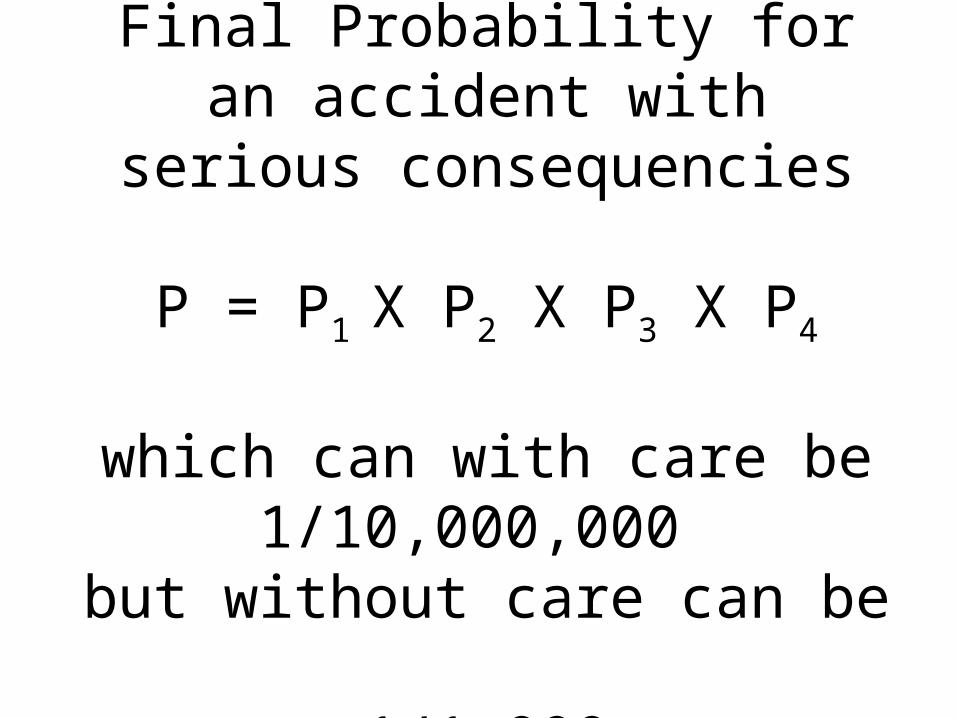
Final Probability for an accident with serious consequencies
P = P1 X P2 X P3 X P4
which can with care be 1/10,000,000
but without care can be 1/1,000
Simple Fault tree

ASSUMPTIONS
(1) We have drawn all possible trees with consequencies
(2) The probabilities are independent (design to make them so; look very
carefully about correlations(3) Consider carefully - with some confidentiality - actions that can artificially correlate the separate
probabilities
The event tree analysis SHOULD have been used by NASA in the
1980s and it would have avoided the Challenger disaster
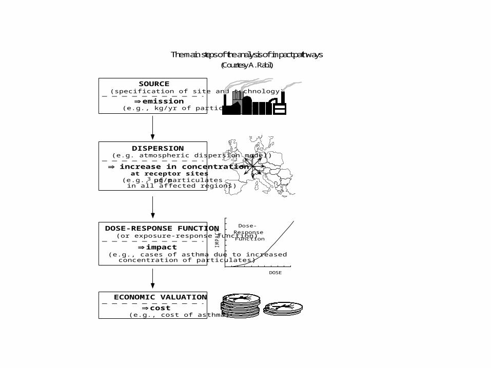
The main steps of the analysis of impact pathways(Courtesy A. Rabl).
DOSE
IMPA
CT
Dose-ResponseFunction
impact(e.g., cases of asthma due to increased
concentration of particulates)
DOSE-RESPONSE FUNCTION(or exposure-response function)
cost(e.g., cost of asthma)
ECONOMIC VALUATION
DISPERSION(e.g. atmospheric dispersion model)
emission(e.g., kg/yr of particulates)
increase in concentrationat receptor sites
(e.g., µg/m3 of particulatesin all affected regions)
SOURCE(specification of site and technology)
Example: Risk of a Space Probe
major risk:Probe (powered by Plutonium) reenters the earth’s atmosphere
burns up spreads its plutonium widely over
everyoneCauses an increase in lung cancer
2 Steps(1) What is the probability of reentry
(2) What is the distribution of Plutonium
Compare with what we know