risk and the extent of insurance - world bank
TRANSCRIPT

Background Paper
Risk and the extent of Insurance Garance Genicot Georgetown University Ethan Ligon Berkeley University

RISK AND THE EXTENT OF INSURANCE
GARANCE GENICOT & ETHAN LIGON
1. Introduction
Households in developing countries are exposed to substantial income risk (weather, crop,price, illnesses, crime, etc.), and have been shown to engage in costly strategies to managethese risks. The two pillars of risk management are risk reduction and risk coping strategies.Risk avoidance and diversi�cation try to reduce income risk, while coping mechanisms suchas savings, borrowing and transfers insure household consumption against income risk.
In this paper, we propose a measure of the extent of insurance which assesses the e�cacyof these coping mechanisms. We measure insurance by contrasting the expected utility ofconsumption an individual has with the utility that she would have if she were to consumeher income in each period (adjusted to account for the price of these coping mechanisms). Weshow that in the case of the log utility, our measure of insurance corresponds to the di�erencebetween the amount of income risk a household bears, and the amount of consumption riskit faces.
To be sure, a household with no income risk will not have any insurance�there's simply nohazard for the household to insure itself against. In contrast, a household with a high levelof income risk can be seen to have a high level of insurance if the household's consumptionrisk is low, and a low level of insurance if consumption risk is high.
There are di�erent advantages to measuring risk and insurance in terms of utility loss andgain respectively. First, it makes it possible to jointly consider many sources of uncertainty.Second, all �uctuations in income are considered and for households of all income levels. Thisis in contrast to a large literature on risk and vulnerability considering only some negativeshocks or only shocks bringing income below a given poverty level.1. Third, a utility functionwith decreasing risk aversion naturally takes into account that, everything else being equal,the cost of uncertainty is lower for richer households. We contrast our measures using alogarithmic utility and a quadratic utility. In the latter case, our measure of insurance isproportional to the di�erence between adjusted income and consumption variance and hasthe undesirable properties to increase in income and to be highly responsive to even smallamounts of risk.
Next, we take these concepts to the data. Using data from four waves of the IndonesiaFamily Life Survey (IFLS), we measure income risk, consumption risk and insurance. Firstwe estimate household speci�c parameters for a lognormal distribution of income. Under logutility, we �nd that the average household faces an income risk is 0.28, implying a utilityloss of 4 percent in the absence of any means of smoothing. Next, assuming a log normal
1See among others Calvo and Dercon (2013)1

distribution of income and a linear relationship between log income and log consumption(following Jalan and Ravallion (1999)), we estimate an elasticity of consumption responseto income shock of about 9 percent. For the average household, we �nd a consumption riskbelow 0.11 or a utility loss of less than 2 percent from not fully smoothing consumption.This implies a level of insurance for the average household of at least 0.17, more than 60percent of the income risk, though this smoothing might come at a substantial price in termsof average consumption.
Comparing across households, we �nd that education and a rural location are importantdeterminants of the risk and insurance for households. Rural households face substantiallymore income risk than urban households, though they bene�t from more insurance at alower cost. Education does reduces both the income risk and the insurance for our IFLShouseholds.
This paper is related to a large literature in development on risk and vulnerability (see amongothers Dercon (2001), Ligon and Schechter (2003), (2004), Ligon (2010)) and on testing theextent of risk sharing among individuals in a community (Deaton, 1992; Townsend, 1994;Udry, 1994; Jalan and Ravallion, 1999; Ligon et al., 2002; Grimard, 1997; Gertler and Gruber,2002). In addition, there is also a large related literature in macroeconomics measuring thee�ect of income shocks on consumption (see among others Krueger and Perri, 2005; Heathcoteet al., 2010)) and calibrating di�erent models of risk sharing (Kaplan and Violante, 2009).
The paper is organized as follows. In the next Section, we formalize the concept of risk andthe extent of insurance against that risk. Section 3 provides some examples. Sections 4 and5 present our estimations using Indonesian longitudinal data. Finally Section 6 concludes.
2. Risk and the Extent of Insurance
In this Section, we propose a way to conceptually de�ne measures of insurance, income andconsumption risk from a household's point of view.
Consider an environment in which a household can choose one of S di�erent income processes.Think of these as corresponding to di�erent choices of crops, occupations, or locations andcapturing not only the opportunities but also the means of ex-ante diversi�cation availableto that particular household. The household is not permitted to choose a combination ofthese income processes.
The household has an increasing, concave utility function u : R→ R, and seeks to maximizeits expected utility of consumption. The choice of an income process s depends on the ul-timate distribution of consumption associated with this process. Given a choice of the sthincome process, the di�erent means of consumption smoothing available for the householdde�ne a correspondence Cs from the income process s to a set of possible consumption distri-butions.2 Let Gs be the distribution of consumption that maximizes the household expectedutility of consumption for a given income process s and Esu(c) the resulting expected utilityof consumption. The household chooses the income process s that maximizes Esu(c). Next,
2To be sure, the means of smoothing available to the household depend in general on the income processs itself. For instance, the performance of informal risk sharing agreements are highly dependent on theobservability and variability of the income process.
2

given this choice, we de�ne the observed �insurance adjusted risk� to the household as theincome risk it faces minus the insurance from which it bene�ts, net of its cost.
First, we de�ne the income risk. Denote as Esy the household's expected income given itsincome process s. Now suppose that the household was faced with the prospect of simplyconsuming its income. Then because the household is risk-averse, it would prefer to haveEsy with certainty, rather than only in expectation. Hence, we can de�ne the income risk
to which the household is exposed by
(1) Is ≡ u(Esy)− Esu(y).
This is simply the loss of utility the household would face if it had to consume its realizedincome instead of its expected income. It contrasts u(Esy) an individual's utility under theArrow-Debreu model, in which complete and perfectly competitive markets allow individualsto fully insure themselves at actuarially fair prices, to Esu(y), its utility if �nancial assetsare entirely absent and consumption bears all the adjustment to income shocks. By Jensen'sinequality, income risk is necessarily non-negative.
Second, we de�ne the insurance and its cost. Though the household is exposed to incomerisk, in general it takes actions to make its consumption smoother than its income (byusing formal or informal insurance or credit markets). In other words, the distribution ofconsumption Gs generally di�ers from the income distribution given s. Denote as Esc theexpected consumption given Gs. Since a risk-averse household is willing to sacri�ce someexpected consumption in exchange for less variable consumption, we may have Esc < Esyeven if Esu(c) > Esu(y). Call the ratio Esc/Esy the �loss ratio�, or Ls. (In the benchmarkArrow-Debreu model with complete and perfect insurance markets, Ls will be one.) Onecan think of
Ps ≡ Esu(y)− Esu(yLs)
as the (utility) premium for insurance.
Now, provided that consumption is less variable than income (in the sense that c is a mean-preserving spread of ysLs), then from Rothschild and Stiglitz (1970) and the concavity of uwe know that
Esu(c) ≥ Esu(yLs).
De�ne the di�erence of these two to be �insurance,� and denote the level of insurance for ahousehold with income process s by
(2) As ≡ Esu(c)− Esu(yLs).
Note that a more insured household isn't necessarily a household with higher expected utility.There's a trade-o� between being well-insured and having a high expected consumption, andin some environments, smoothing consumption may be very expensive. In some ways thismay be unappealing: the insurance of the household in e�ect depends on both how muchvariation there is in income and consumption, and on the loss ratio. The loss ratio in turndepends on the e�ciency with which insurance is provided in the household's environment.
Putting this all together, the insurance adjusted risk that the household ends up facing isgiven by
Is + Ps − As = u(Esy)− Esu(c).3

Finally, notice that we measure the insurance-adjusted risk that the household ends up facinggiven its choice of income process. This does not include the cost of diversi�cation, wherebythe household trades opportunities for a lower risk (selects an income process s that doesnot maximize Esy). This cost of diversi�cation can be substantial in environments with verylimited or costly insurance, but would be very hard to empirically measure. This is why wefocus on the insurance adjusted risk actually faced by the household.
3. Examples
In this Section, we turn to examples that illustrate our concepts of risk and insurance invarious settings. Table 1 summarizes the �ndings.
3.1. Logarithmic Utility. For the case in which u(c) = log(c) the utility premium forinsurance and insurance itself take a particularly nice form. The loss ratio of course dependsjust on expected income and consumption. And with log utility, Esu(yLs) = Es log(y) +log(Esc)− log(Esy). Thus, we can write insurance as
(3) As = [u(Esy)− Esu(y)]− [u(Esc)− Esu(c)].
Thus, in the jargon above �insurance� is equal to income risk minus consumption risk in thelogarithmic case. Note that if households perfectly smooth their consumption (so that thelast bracketed term, consumption risk, is zero) then insurance completely compensates forincome risk.
3.2. Random endowments with precautionary savings. Consider �ve households,each with logarithmic utility. Each household has a di�erent endowment process, but allhave the same mean of 1.25 in every period.
3.2.1. Household A. Household A receives a �xed endowment of 1.25 every period for sure, sohis income risk is (u(Ey)−E(u(y)) is zero. The household consumes exactly that endowment,so that every period he has a utility of Eu(c) = log(1.25) ≈ 0.223, and a residual consumption
risk of Eu(c) − u(Ec) = 0. With a loss ratio of zero, the household's insurance is equal toits income risk minus its consumption risk; in this case both are zero, so insurance is zero.This household simply has no need for insurance.
3.2.2. Household B. Household B is an autarkist. She receives an endowment of either 1/2or 2, each with probability 1/2�note that the mean endowment for the second household isalso 1.25. This household's risk income risk is (u(Ey)− E(u(y)) = log(1.25)− 1
2[log(1/2) +
log(2)] ≈ 0.223. Because this autarkic household does nothing to reduce the e�ect of theseendowment shocks on consumption, its consumption risk is equal to its exposure, and itsinsurance is also zero. This household would bene�t from insurance, but for some reasonhas none.
4

Table1.Decom
positionof
Insurance
Adjusted
Risk
Insurance
adjusted
risk
Lossratio(L
s)
Incomerisk
(Is)
Premium
(Ps)
Insurance
(As)
GeneralExpression
u(E
sy)−Esu
(c)
Esc/Esy
u(E
sy)−Esu
(y)
Esu
(y)−Esu
(yLs)
Esu
(c)−Esu
(yLs)
HouseholdA
01
00
0HouseholdB
≈0.
223
1≈
0.22
30
0HouseholdC
01
≈0.
223
0≈
0.22
3HouseholdD
>0
0.88
≈0.
223
≈0.
056
0.17
3HouseholdE
>0
<1
≈0.
223
>0
<0.
223
logutility...
log(E
sy)−
Eslo
g(c
)Esc/Esy
log(E
sy)−
Eslo
g(y
)lo
g(E
sy)−
log(E
sc)
I s−
[log
(Esc)−
Eslo
g(c
)]
...&
JRcons...
log(E
sy)−α
eα−βµsEsyβ
Esy
log(E
sy)−µs
log(E
sy)−
log(E
sc)
I s−
[log
(Esc)−α
]
...&
lognormaly
µs
+σ
2 s/2−α
exp(α−µs
+(β
2−
1)σ
2 s 2)
σ2 s/2
µs−α
+(1−β
2)σ
2 s/2
(1−β
2)σ
2 s/2
Stone-Geary
utility
log(E
sy−
φ)−
Eslo
g(c−φ
)Esc/Esy
log(E
sy−
φ)−
Eslo
g(y−φ
)lo
g(E
sy−
φ)−
log(E
sc−φ
)I s−
[log
(Esc−φ
)−
Eslo
g(c−φ
)]Indonesia(µ
i=µ)
0.6
[0.5
5,0.
63]
0.29
[0.5
9,0.
65]
[0.1
5,0.
28]
5
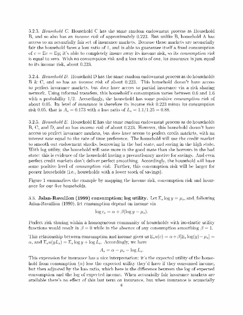
3.2.3. Household C. Household C has the same random endowment process as HouseholdB, and so also has an income risk of approximately 0.223. But unlike B, household A hasaccess to an actuarially fair set of insurance markets. Because these markets are actuariallyfair the household faces a loss ratio of 1, and is able to guarantee itself a �xed consumptionof c = Ec = Ey; it's able to completely insure away its income risk, so its consumption risk
is equal to zero. With no consumption risk and a loss ratio of one, its insurance is just equalto its income risk, about 0.223.
3.2.4. Household D. Household D has the same random endowment process as do householdsB & C, and so has an income risk of about 0.223. This household doesn't have accessto perfect insurance markets, but does have access to partial insurance via a risk sharingnetwork. Using informal transfers, this household's consumption varies between 0.6 and 1.6with a probability 1/2. Accordingly, the household has some positive consumption risk ofabout 0.05. Its level of insurance is therefore its income risk 0.223 minus its consumptionrisk 0.05, that is As = 0.173 with a loss ratio of Ls = 1.1/1.25 = 0.88.
3.2.5. Household E. Household E has the same random endowment process as do householdsB, C, and D, and so has income risk of about 0.223. However, this household doesn't haveaccess to perfect insurance markets, but does have access to perfect credit markets, with aninterest rate equal to the rate of time preference. The household will use the credit marketto smooth out endowment shocks, borrowing in the bad state, and saving in the high state.With log utility, the household will save more in the good state than she borrows in the badstate: this is evidence of the household having a precautionary motive for savings. And evenperfect credit markets don't deliver perfect smoothing. Accordingly, the household will havesome positive level of consumption risk. Further, this consumption risk will be larger forpoorer households (i.e., households with a lower stock of savings).
Figure 1 summarizes the example by mapping the income risk, consumption risk and insur-ance for our �ve households.
3.3. Jalan-Ravallion (1999) consumption; log utility. Let Es log y = µs, and, followingJalan-Ravallion (1999), let consumption depend on income via
log cs = α + β(log y − µs).
Perfect risk sharing within a homogeneous community of households with iso-elastic utilityfunctions would result in β = 0 while in the absence of any consumption smoothing β = 1.
This relationship between consumption and income gives us Esu(c) = α+β[Es log(y)−µs] =α, and Esu(yLs) = Es log y + logLs. Accordingly, we have
As = α− µs − logLs.
This expression for insurance has a nice interpretation: it's the expected utility of the house-hold from consumption (α) less the expected utility they'd have if they consumed income,but then adjusted by the loss ratio, which here is the di�erence between the log of expectedconsumption and the log of expected income. When actuarially fair insurance markets areavailable there's no e�ect of this last term on insurance, but when insurance is actuarially
6

A
Inco
me
Ris
k
Cons. Risk
Insu
ranc
e=
0
0.05 0.223
0.223B
CD
Insurance
Figure 1. Illustration of Relation Between Insurance and In-come/Consumption Risk
unfair there's a trade-o� between the smoothness of consumption and its level (in expecta-tion).
3.3.1. Adding log-normal income. If we further assume that log y ∼ N(µs, σ2s), then we
can calculate a simple parametric expression for insurance. We already have Esu(c) = αand Esu(y) = µs. By using the log-normal distributional assumption we also know thatEsy = eµs+σ
2s/2, and that Esc = eα+β2σ2
s/2.
Now, �rst, using the two terms involving the income process, we then have that income riskis equal to σ2
s/2, and consumption risk is simply β2σ2
s/2. Then substituting all of these termsinto (3) gives
As = (1− β2)σ2s
2.
7
Once again, this has a nice interpretation. Insurance in this example is equal to the productof income risk (σ2
s/2) and the proportion of income risk which is left uninsured (1− β2).
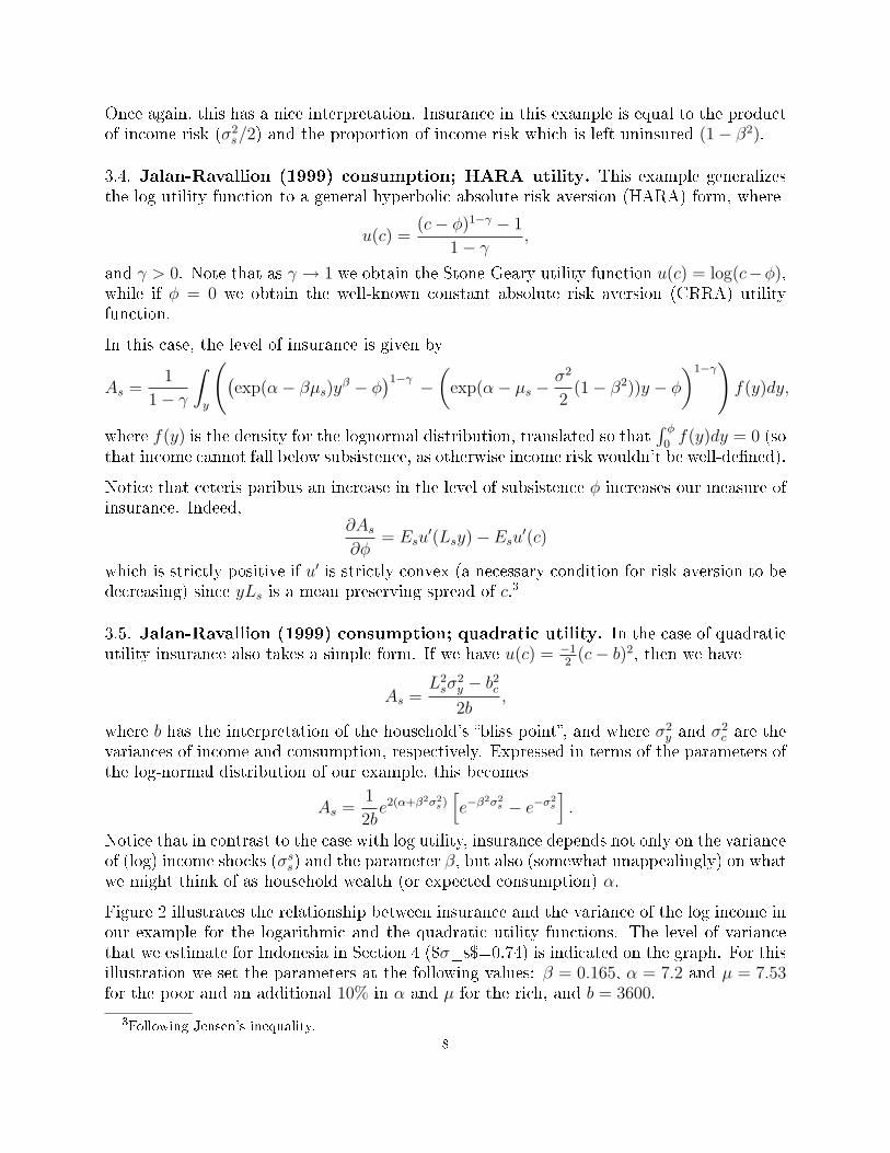
3.4. Jalan-Ravallion (1999) consumption; HARA utility. This example generalizesthe log utility function to a general hyperbolic absolute risk aversion (HARA) form, where
u(c) =(c− φ)1−γ − 1
1− γ,
and γ > 0. Note that as γ → 1 we obtain the Stone-Geary utility function u(c) = log(c−φ),while if φ = 0 we obtain the well-known constant absolute risk aversion (CRRA) utilityfunction.
In this case, the level of insurance is given by
As =1
1− γ
∫y
((exp(α− βµs)yβ − φ
)1−γ − (exp(α− µs −σ2
2(1− β2))y − φ
)1−γ)f(y)dy,
where f(y) is the density for the lognormal distribution, translated so that∫ φ
0f(y)dy = 0 (so
that income cannot fall below subsistence, as otherwise income risk wouldn't be well-de�ned).
Notice that ceteris paribus an increase in the level of subsistence φ increases our measure ofinsurance. Indeed,
∂As∂φ
= Esu′(Lsy)− Esu′(c)
which is strictly positive if u′ is strictly convex (a necessary condition for risk aversion to bedecreasing) since yLs is a mean preserving spread of c.3
3.5. Jalan-Ravallion (1999) consumption; quadratic utility. In the case of quadraticutility insurance also takes a simple form. If we have u(c) = −1
2(c− b)2, then we have
As =L2sσ
2y − b2c2b
,
where b has the interpretation of the household's �bliss point�, and where σ2y and σ
2c are the
variances of income and consumption, respectively. Expressed in terms of the parameters ofthe log-normal distribution of our example, this becomes
As =1
2be2(α+β2σ2
s)[e−β
2σ2s − e−σ2
s
].
Notice that in contrast to the case with log utility, insurance depends not only on the varianceof (log) income shocks (σss) and the parameter β, but also (somewhat unappealingly) on whatwe might think of as household wealth (or expected consumption) α.
Figure 2 illustrates the relationship between insurance and the variance of the log income inour example for the logarithmic and the quadratic utility functions. The level of variancethat we estimate for Indonesia in Section 4 ($σ_s$=0.74) is indicated on the graph. For thisillustration we set the parameters at the following values: β = 0.165, α = 7.2 and µ = 7.53for the poor and an additional 10% in α and µ for the rich, and b = 3600.
3Following Jensen's inequality.8

As(σ
s)
σs
Indonesia
Indonesia
Indonesia
As(σs) (quadratic utility; poor)
As(σs) (log utility)
As(σs) (quadratic utility; wealthy)
Figure 2. Insurance as a function of σs for log and quadratic utility. ForIndonesia, we estimate that β = 0.165 and σs = 0.75.
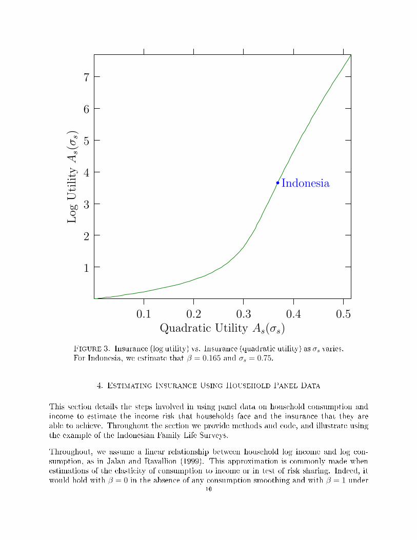
The assumption of increasing risk aversion implicit in the quadratic utility results in highermeasures of insurance for rich households than for poor households. We also see that witha logarithmic utility the value of insurance is quadratic in the standard deviation of the logincome σs while it grows more than exponentially with it in the case of the quadratic utility,perhaps over-evaluating the value of insurance when there is little risk. This is clearly shownin Figure 3 which plots the insurance level measured using the log utility and insurancemeasured using a quadratic utility for di�erent values of σs. For these reasons, the quadraticutility function appears to be a particularly unattractive choice of utility function in thiscontext and we will favor the logarithmic utility in our empirical exercise.
9
1
2
3
4
5
6
7Log
Uti
lity
As(σ
s)
0.1 0.2 0.3 0.4 0.5Quadratic Utility As(σs)
Indonesia
Figure 3. Insurance (log utility) vs. Insurance (quadratic utility) as σs varies.For Indonesia, we estimate that β = 0.165 and σs = 0.75.
4. Estimating Insurance Using Household Panel Data
This section details the steps involved in using panel data on household consumption andincome to estimate the income risk that households face and the insurance that they areable to achieve. Throughout the section we provide methods and code, and illustrate usingthe example of the Indonesian Family Life Surveys.
Throughout, we assume a linear relationship between household log income and log con-sumption, as in Jalan and Ravallion (1999). This approximation is commonly made whenestimations of the elasticity of consumption to income or in test of risk sharing. Indeed, itwould hold with β = 0 in the absence of any consumption smoothing and with β = 1 under
10

perfect risk sharing within a homogeneous community of households with iso-elastic utilityfunctions. We also maintain our assumption of logarithmic utility.
We index di�erent households in the panel dataset by i = 1, . . . , N , and periods by t =1, . . . , T . We assume that a given household chooses a particular income process at or beforetime t = 1, and operates that same income process for at least the T periods over whichthe household is observed in the data. Similarly, we assume that the relationship betweenconsumption and income is unchanging over this interval.
The data used are described in greater detail in Data from the Indonesian Family LifeSurvey (IFLS), where we discuss di�erent sources of income and consumption and how theseare measured and aggregated. For the purposes of analysis, we use income from all reportedsources (business income, labor earnings, asset income, and other income sources) but excludeincome received as transfers from other individuals, on the grounds that these may in factbe credit or insurance used to smooth consumption. For our measure of consumption werestrict attention to food expenditures (including the estimated value of food produced athome, but excludes outside meals, data for which weren't collected in a consistent manneracross all rounds of the survey). Household income or consumption is treated as a per capitaquantity by simply dividing by the number of people resident in the household at the timeof the survey, and it is generally this per capita measure of income or consumption that werely on in the analysis below.
4.1. Estimating the distribution of income. As in our examples above, we assume thathousehold income yi follows a log-normal distribution with a mean (of logs) of µi and avariance σ2
i . Note that we allow for both household-speci�c means and for heteroskedasticincome shocks. In the Indonesian case we estimate the relationship between the mean of(log) income and its variance by computing the household-speci�c means and examining thedistribution of the residuals. Figure 4 shows the scatterplot of squared log income shocksplotted against the estimated µi. We estimate the regression
(4) (log yit − µi)2 = a0 + a1µi + a2(µi − µ)2 + εit,
where µ = N−1∑N
i=1 µi. Results are reported in the following table, and a graph of theestimated relationship given in Figure 4. A null hypothesis of equal variances is stronglyrejected, so we use these results to allow for a heteroskedastic income distribution, withlog yi ∼ N (µi, 2.10− 0.26µi + 0.19(µi − µ)2).
Coe�. Std. Err.Constant 2.099 0.065µi -0.257 0.011(µi − µ)2 0.192 0.007
Figure 5 illustrates the distribution of both the mean terms in the cross-section and of log-income across both households and rounds. The total variance of log income is 1.89. Ofthis overall variance in log income, the cross-sectional variance of the {µi} is 1.08; thuscross-sectional variation accounts for 56% of the overall variation in log income.
We can use our estimates of the variance of log income shocks along with our assumptionthat these shocks are distributed log-normal to estimate expected income for household i as a
11
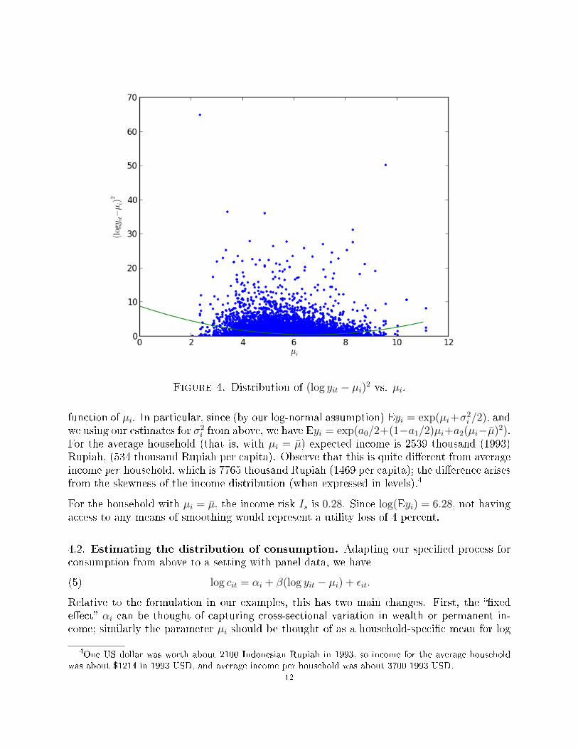
Figure 4. Distribution of (log yit − µi)2 vs. µi.
function of µi. In particular, since (by our log-normal assumption) Eyi = exp(µi+σ2i /2), and
we using our estimates for σ2i from above, we have Eyi = exp(a0/2+(1−a1/2)µi+a2(µi−µ)2).
For the average household (that is, with µi = µ) expected income is 2539 thousand (1993)Rupiah, (534 thousand Rupiah per capita). Observe that this is quite di�erent from averageincome per household, which is 7765 thousand Rupiah (1469 per capita); the di�erence arisesfrom the skewness of the income distribution (when expressed in levels).4
For the household with µi = µ, the income risk Is is 0.28. Since log(Eyi) = 6.28, not havingaccess to any means of smoothing would represent a utility loss of 4 percent.
4.2. Estimating the distribution of consumption. Adapting our speci�ed process forconsumption from above to a setting with panel data, we have
(5) log cit = αi + β(log yit − µi) + εit.
Relative to the formulation in our examples, this has two main changes. First, the ��xede�ect� αi can be thought of capturing cross-sectional variation in wealth or permanent in-come; similarly the parameter µi should be thought of as a household-speci�c mean for log
4One US dollar was worth about 2100 Indonesian Rupiah in 1993, so income for the average householdwas about $1214 in 1993 USD, and average income per household was about 3700 1993 USD.
12
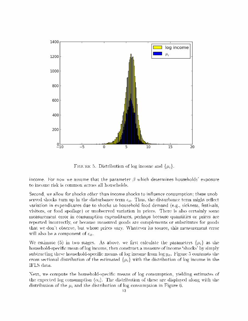
Figure 5. Distribution of log income and {µi}.
income. For now we assume that the parameter β which determines households' exposureto income risk is common across all households.
Second, we allow for shocks other than income shocks to in�uence consumption; these unob-served shocks turn up in the disturbance term εit. Thus, the disturbance term might re�ectvariation in expenditures due to shocks to household food demand (e.g., sickness, festivals,visitors, or food spoilage) or unobserved variation in prices. There is also certainly somemeasurement error in consumption expenditures, perhaps because quantities or prices arereported incorrectly, or because measured goods are complements or substitutes for goodsthat we don't observe, but whose prices vary. Whatever its source, this measurement errorwill also be a component of εit.
We estimate (5) in two stages. As above, we �rst calculate the parameters {µi} as thehousehold-speci�c mean of log income, then construct a measure of income `shocks' by simplysubtracting these household-speci�c means of log income from log yit. Figure 5 contrasts thecross sectional distribution of the estimated {µi} with the distribution of log income in theIFLS data.
Next, we compute the household-speci�c means of log consumption, yielding estimates ofthe expected log consumption (αi). The distribution of these are displayed along with thedistribution of the µi and the distribution of log consumption in Figure 6.
13

Figure 6. Distribution of expected log income and consumption.
As is evident from the �gure, the variance of αi (0.33) is considerably smaller than thevariance of µi (1.08). But of course this variation doesn't bear directly on matters of risk orinsurance for a given household, but rather is an indication that inequality in consumption issmaller than inequality in income, as is to be expected when households are able to smooththeir consumption relative to their income.
Figure 7 illustrates the connection between shocks to log income and the consumption re-sponse, estimating
log cit − αi = β(log yit − µi) + εit.
The resulting estimate of β is 0.165, with a standard error of 0.003. The magnitude of thisestimated coe�cient is roughly in line with other estimates in the risk-sharing literature(Townsend, 1994; Gertler and Gruber, 2002), where, as a rule of thumb the elasticity ofconsumption response to income shock is typically in the neighborhood of 5�15%, but lowerthan the 18% found by Jalan and Ravallion in China. And as we've seen, the varianceof income shocks is large compared to the variance of consumption shocks, so there's nodoubt that income shocks are of considerable economic importance for household welfare inIndonesia.
For our present exercise, this estimated elasticity between income and consumption shocks isof central importance to understanding the extent of insurance. Recall that with log utility,
14
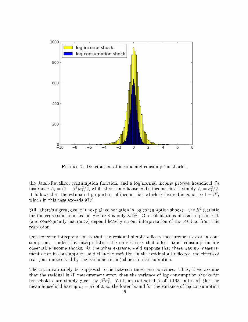
Figure 7. Distribution of income and consumption shocks.
the Jalan-Ravallion consumption function, and a log normal income process household i'sinsurance Ai = (1 − β2)σ2
i /2, while that same household's income risk is simply Is = σ2i /2.
It follows that the estimated proportion of income risk which is insured is equal to 1 − β2,which in this case exceeds 97%.
Still, there's a great deal of unexplained variation in log consumption shocks�the R2 statisticfor the regression reported in Figure 8 is only 3.1%. Our calculations of consumption risk(and consequently insurance) depend heavily on our interpretation of the residual from thisregression.
One extreme interpretation is that the residual simply re�ects measurement error in con-sumption. Under this interpretation the only shocks that a�ect `true' consumption areobservable income shocks. At the other extreme, we'd suppose that there was no measure-ment error in consumption, and that the variation in the residual all re�ected the e�ects ofreal (but unobserved by the econometrician) shocks on consumption.
The truth can safely be supposed to lie between these two extremes. Thus, if we assumethat the residual is all measurement error, then the variance of log consumption shocks forhousehold i are simply given by β2σ2
i . With an estimated β of 0.165 and a σ2i (for the
mean household having µi = µ) of 0.56, the lower bound for the variance of log consumption15

Figure 8. Distribution of income and consumption shocks.
shocks is 0.027. The upper bound (assuming no measurement error in consumption) is justthe sample variance of log consumption shocks, or 0.27.
With these upper and lower bound estimates of the variance of log consumption shocks, andassuming that residuals and income are distributed log normal, we can construct upper andlower bound estimates of other quantities necessary to compute consumption risk, insurance,and so on. In particular, we have
Eci = exp
[αi +
β2
2σ2i +
σ2ε
2
],
where σ2ε is the variance of the �true� disturbance to log consumption (i.e., excluding mea-
surement error). Setting this σ2ε = 0 gives us a lower bound estimate of the true value of
expected consumption for household i. Choosing the mean household, which we've de�nedthis household as one with µi = µ ≈ 6.0 and then using the formula from Figure 6 impliesthat this same mean household has αi = 5.62.
Now, substituting the values we've computed for this mean household, we can substitute toget an estimate of Eci. If σ2
ε = 0 then we get lower bound estimate of Eci ≈ exp[5.62 +0.172(0.29)] = 278 thousand (1993) Rupiah of food consumption per person. The upperbound involves multiplying the lower bound times eσ
2ε /2, where σ2
ε takes a maximum value of0.27; thus, the upper bound estimate of expected food consumption for the mean household is
16

Table 2. Values of key quantities in the IFLS data
µ 5.91σ2i (µi = µ) 0.58α 5.6#Households 15030.0Total Obs. 38117.0Avg. Consumption/Person 374.19Var. log cons. shocks 0.27Var. log income shocks 0.84β 0.17Lower bound of Eci (µi = µ) 271.87Upper bound of Eci (µi = µ) 311.64Eyi (µi = µ) 492.32Lower bound of loss ratio 0.55Upper bound of loss ratio 0.63Upper bound of Insurance 0.15Lower bound of Insurance 0.28Ins. adj. risk (µi = µ) 0.6
312 thousand (1993) Rupiah. As with income, expected consumption for the mean householdis considerably lower than average consumption per household (372), re�ecting the skeweddistribution of consumption across households.
Because there's a range of possible values for expected consumption, there's also a rangefor possible values of the loss ratio Eci/Eyi. For the household with µi = µ we've alreadycalculated the denominator of this expression (Eyi = 492), and we've already calculated therange of possible values for the numerator [272, 312], so that the range of values for the lossratio is [0.55, 0.63]. With log utility, the premium Pi is just equal to minus the logarithm ofthe loss ratio, so for this same household the premium is in the range [0.46, 0.60].
Insurance for a household with log utility and log-normally distributed income will haveinsurance equal to αi − µi − log(Eci) + log(Ey). With the Jalan-Ravallion consumptionfunction we've already computed a range for Eci for the average household. Substitutingthese values into our expression for insurance gives us a range [0.15, 0.28].
Finally, the insurance adjusted risk has the nice feature that in the log case our calculationdoes not depend on our interpretation of the residual in the Jalan-Ravallion regression.Instead we need only to calculate the log of the expected value of income and subtractthe expected utility of consumption, and in the log-normal case this is simply equal toµi + σ2
i /2− αi, or in our case 0.6.
5. Distribution of Insurance Across Households
In the previous section we showed how to compute insurance and other statistics for anaverage household. Here we use the same data from the IFLS but compute insurance andrelated statistics for every household in the dataset.
17
For any given household i, our estimate of its insurance depends on both variables peculiar tothe household and on the distribution of variables across the population. Variables peculiarto the household include realizations of the logs of income and consumption, which forhousehold i are averaged across time to obtain estimates of µi and αi.
Other quantities depend on the distribution of income and consumption across the popula-tion, and come from the estimation of the parameter β in the Jalan-Ravallion consumptionfunction, and of the parameters (a0, a1, a2) in (4) which relates the variance in expected logincome to its mean.
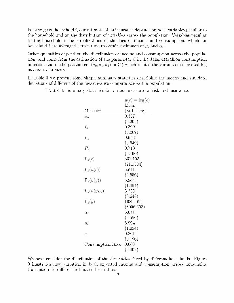
In Table 3 we present some simple summary statistics describing the means and standarddeviations of di�erent of the measures we compute across the population.
Table 3. Summary statistics for various measures of risk and insurance.
u(c) = log(c)Mean
Measure (Std. Dev)As 0.387
(0.205)Is 0.390
(0.207)Ls 0.653
(0.549)Ps 0.710
(0.790)Es(c) 331.105
(211.384)Es(u(c)) 5.641
(0.556)Es(u(y)) 5.964
(1.054)Es(u(yLs)) 5.255
(0.648)Es(y) 1089.165
(6006.393)αi 5.641
(0.556)µi 5.964
(1.054)σ 0.861
(0.196)Consumption Risk 0.003
(0.002)
We next consider the distribution of the loss ratios faced by di�erent households. Figure9 illustrates how variation in both expected income and consumption across householdstranslates into di�erent estimated loss ratios.
18
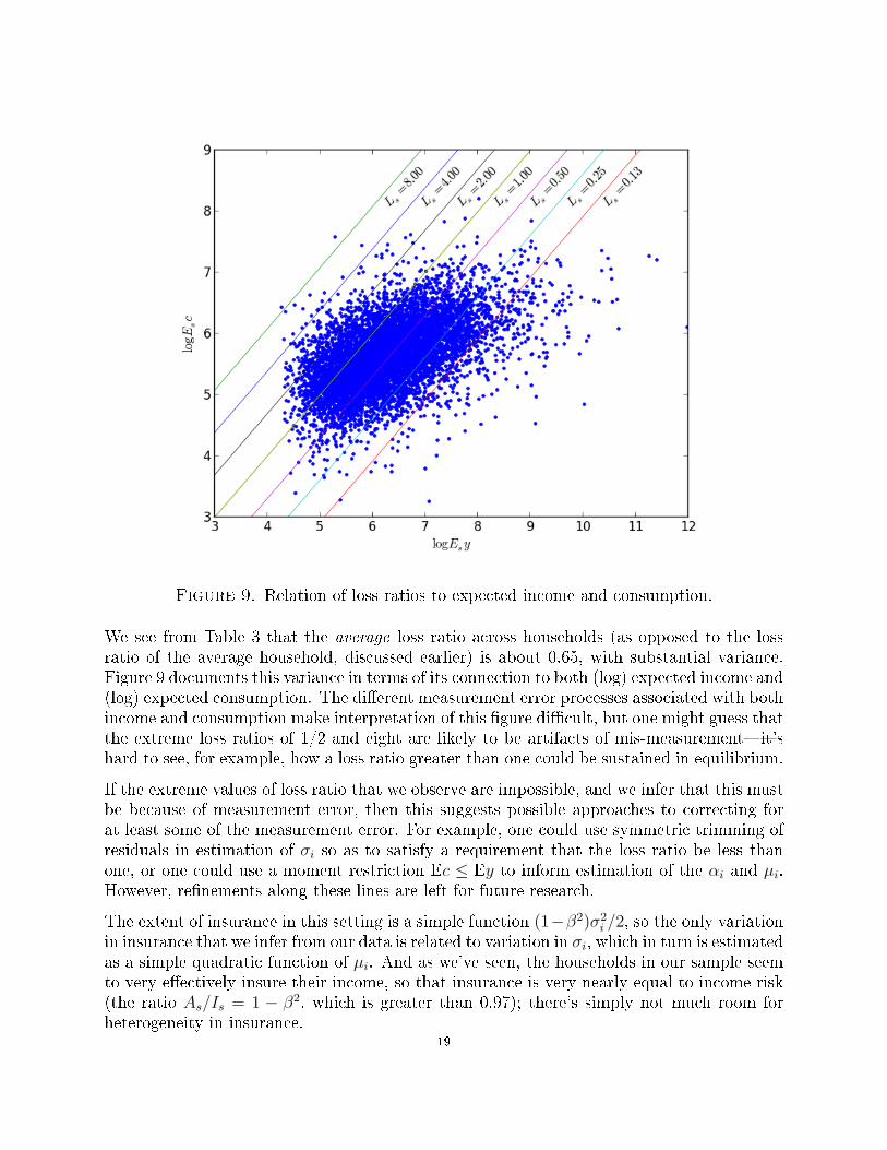
Figure 9. Relation of loss ratios to expected income and consumption.
We see from Table 3 that the average loss ratio across households (as opposed to the lossratio of the average household, discussed earlier) is about 0.65, with substantial variance.Figure 9 documents this variance in terms of its connection to both (log) expected income and(log) expected consumption. The di�erent measurement error processes associated with bothincome and consumption make interpretation of this �gure di�cult, but one might guess thatthe extreme loss ratios of 1/2 and eight are likely to be artifacts of mis-measurement�it'shard to see, for example, how a loss ratio greater than one could be sustained in equilibrium.
If the extreme values of loss ratio that we observe are impossible, and we infer that this mustbe because of measurement error, then this suggests possible approaches to correcting forat least some of the measurement error. For example, one could use symmetric trimming ofresiduals in estimation of σi so as to satisfy a requirement that the loss ratio be less thanone, or one could use a moment restriction Ec ≤ Ey to inform estimation of the αi and µi.However, re�nements along these lines are left for future research.
The extent of insurance in this setting is a simple function (1−β2)σ2i /2, so the only variation
in insurance that we infer from our data is related to variation in σi, which in turn is estimatedas a simple quadratic function of µi. And as we've seen, the households in our sample seemto very e�ectively insure their income, so that insurance is very nearly equal to income risk(the ratio As/Is = 1 − β2, which is greater than 0.97); there's simply not much room forheterogeneity in insurance.
19
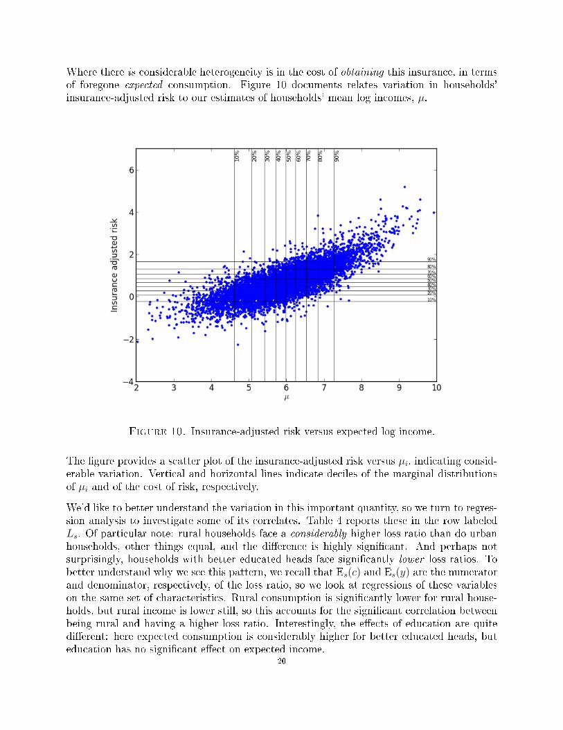
Where there is considerable heterogeneity is in the cost of obtaining this insurance, in termsof foregone expected consumption. Figure 10 documents relates variation in households'insurance-adjusted risk to our estimates of households' mean log incomes, µ.
Figure 10. Insurance-adjusted risk versus expected log income.
The �gure provides a scatter plot of the insurance-adjusted risk versus µi, indicating consid-erable variation. Vertical and horizontal lines indicate deciles of the marginal distributionsof µi and of the cost of risk, respectively.
We'd like to better understand the variation in this important quantity, so we turn to regres-sion analysis to investigate some of its correlates. Table 4 reports these in the row labeledLs. Of particular note: rural households face a considerably higher loss ratio than do urbanhouseholds, other things equal, and the di�erence is highly signi�cant. And perhaps notsurprisingly, households with better educated heads face signi�cantly lower loss ratios. Tobetter understand why we see this pattern, we recall that Es(c) and Es(y) are the numeratorand denominator, respectively, of the loss ratio, so we look at regressions of these variableson the same set of characteristics. Rural consumption is signi�cantly lower for rural house-holds, but rural income is lower still, so this accounts for the signi�cant correlation betweenbeing rural and having a higher loss ratio. Interestingly, the e�ects of education are quitedi�erent: here expected consumption is considerably higher for better educated heads, buteducation has no signi�cant e�ect on expected income.
20
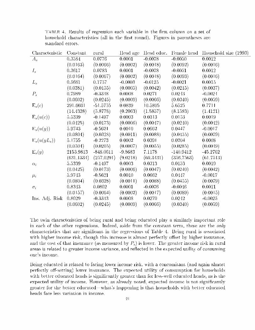
Table 4. Results of regression each variable in the �rst column on a set ofhousehold characteristics (all in the �rst round). Figures in parentheses arestandard errors.
Characteristic Constant rural Head age Head educ. Female head Household size (1993)As 0.3584 0.0776 0.0001 -0.0078 -0.0050 0.0012
(0.0163) (0.0066) (0.0002) (0.0018) (0.0092) (0.0016)Is 0.3617 0.0783 0.0001 -0.0078 -0.0051 0.0012
(0.0164) (0.0067) (0.0002) (0.0018) (0.0093) (0.0016)Ls 0.5661 0.1757 -0.0003 -0.0125 -0.0021 0.0015
(0.0381) (0.0155) (0.0005) (0.0042) (0.0215) (0.0037)Ps 0.7989 -0.3348 0.0008 0.0271 0.0243 -0.0024
(0.0602) (0.0245) (0.0009) (0.0066) (0.0340) (0.0059)Es(c) 291.6031 -51.5755 0.0839 10.5805 5.6525 0.7711
(14.4328) (5.8778) (0.2063) (1.5857) (8.1583) (1.4121)Es(u(c)) 5.5339 -0.1497 0.0003 0.0313 0.0153 0.0019
(0.0425) (0.0173) (0.0006) (0.0047) (0.0240) (0.0042)Es(u(y)) 5.9743 -0.5621 0.0010 0.0662 0.0447 -0.0017
(0.0804) (0.0328) (0.0011) (0.0088) (0.0455) (0.0079)Es(u(yLs)) 5.1755 -0.2273 0.0002 0.0391 0.0204 0.0008
(0.0504) (0.0205) (0.0007) (0.0055) (0.0285) (0.0049)Es(y) 2153.9813 -848.0611 -9.8683 7.1178 -140.9412 -45.2762
(631.1334) (257.0291) (9.0218) (69.3431) (356.7563) (61.7513)αi 5.5339 -0.1497 0.0003 0.0313 0.0153 0.0019
(0.0425) (0.0173) (0.0006) (0.0047) (0.0240) (0.0042)µi 5.9743 -0.5621 0.0010 0.0662 0.0447 -0.0017
(0.0804) (0.0328) (0.0011) (0.0088) (0.0455) (0.0079)σi 0.8343 0.0802 0.0001 -0.0076 -0.0046 0.0011
(0.0157) (0.0064) (0.0002) (0.0017) (0.0089) (0.0015)Ins. Adj. Risk 0.8029 -0.3343 0.0008 0.0270 0.0242 -0.0025
(0.0602) (0.0245) (0.0009) (0.0066) (0.0340) (0.0059)
The twin characteristics of being rural and being educated play a similarly important rolein each of the other regressions. Indeed, aside from the constant term, these are the only
characteristics that are signi�cant in the regressions of Table 4. Being rural is associatedwith higher income risk, though this increase is almost perfectly o�set by higher insurance,and the cost of that insurance (as measured by Ps) is lower. The greater income risk in ruralareas is related to greater income variance, and re�ected in the expected utility of consumingone's income.
Being educated is related to facing lower income risk, with a concomitant (and again almostperfectly o�-setting) lower insurance. The expected utility of consumption for householdswith better educated heads is signi�cantly greater than for less-well educated heads, as is theexpected utility of income. However, as already noted, expected income is not signi�cantlygreater for the better educated�what's happening is that households with better educatedheads face less variation in income.
21

Though households are well-insured, as noted above the cost of insurance exhibits consider-able variation. But from Table 4 we see that rural households face a much lower insurance-adjusted risk than do urban households, while educated households face a higher insurance-adjusted risk. This follows from three facts: (i) rural households have much lower expectedlog income, but (ii) only somewhat lower expected log consumption; despite the fact that(iii) the variance of their income is greater (because this greater variance isn't enough too�set the larger di�erences in the means of log income and consumption).
All this said, it's important to remember that many of the various left-hand-side variablesin the regressions reported in Table 4 are simply functions of a smaller set of parameters.For example, since we're assuming log utility, a log-normal income distribution, and a Jalan-Ravallion consumption function, income risk Is is simply equal to σ
2s/2, which in turn we've
assumed to simply be a quadratic function of µs. And in fact, all of the variation in theleft-hand side variables ultimately depends only on (µs, αs, β, a0, a1, a2), and as noted earlier,only the �rst two of these are household speci�c.
We think that the fact that one can compute sensible measures of insurance, risk, etc.from data on nothing more than income and consumption is an important strength of ourapproach. However, there's no doubt that a more realistic accounting of risk and insurancecould be obtained with richer detail on household characteristics. There are two simple waysin which one could extend what we've done to better allow for observable heterogeneity.
First, though we've been using what we call the Jalan-Ravallion consumption function tomodel the relationship between income and consumption shocks, we've assumed that theentire population shares a single elasticity parameter β governing the co-movement of indi-vidual consumption with income. But a central point of Jalan and Ravallion (1999) is in factthat this elasticity may vary across the population. A simple adaptation of our approachwould estimate di�erent values of β for households with di�erent quantiles of α.
Second, we've estimated the variance of log income shocks σi as a quadratic function ofµi. But one interpretation of the �nal row of Table 4 is that in fact σi also depends onwhether a household is rural or not, and on the education of the household head. So asecond simple adaptation of our approach would involve adding characteristics such as theseto our estimation of the heteroskedasticity of log income.
6. Conclusion
In this paper we make three main contributions.
First, this paper proposes measures of income risk that households face, and of the extent ofinsurance e�ectively delivered by the various coping mechanisms that those households useto minimize the consequence that risk. We measure insurance by contrasting the expectedutility of consumption an individual has with the utility that she would have from consumingher income in each period, adjusted to account for the price of these coping mechanisms. Weshow that, in the log utility case, our measure of insurance boils down to the income risk ahousehold bears minus the consumption risk it faces.
22
Second, we detail the steps necessary to apply these measures to panel data of householdincome and consumption. Third, we measure income risk, consumption risk and insuranceusing four waves of the Indonesia Family Life Survey (IFLS). We show that Indonesianhouseholds face signi�cant income risk but that their various coping mechanism provide themwith a level of insurance representing at the very least 60 percent of the income risk, thoughthis smoothing comes at a large cost in terms of average consumption. Expected consumptionrepresents on average 65 percent of the expected income, suggesting that households arewilling to forgo a non-negligible amount of consumption in order to smooth it. This cost ofinsurance captures most of the utility cost of risk for the IFLS households.
Comparing risk and insurance across households highlights geography and education as keydeterminant of the cost of risk for households. Rural households face higher income riskthan urban household, though they bene�t from more insurance at a lower cost resultingin a lower insurance adjusted risk. Education lowers the income risk faced by households.It also raises the expected log income of households faster than it raises their expected logconsumption resulting in higher insurance adjusted risk for educated households.
7. References
Calvo, G. and S. Dercon (2013). Vulnerability to individual and aggregate poverty. Social
Choice and Welfare.Deaton, A. (1992). Understanding Consumption. Oxford: Clarendon Press.Dercon, S. (2001). Assessing vulnerability. Publication of the Jesus College and CSAE,
Department of Economics, Oxford University .Gertler, P. and J. Gruber (2002). Insuring consumption against illness. American Economic
Review , 51�70.Grimard, F. (1997). Household consumption smoothing through ethnic ties: Evidence fromCote d'Ivoire. Journal of Development Economics 53, 391�422.
Heathcote, J., F. Perri, and G. L. Violante (2010, January). Unequal we stand: An empiricalanalysis of economic inequality in the United States, 1967-2006. Review of Economic
Dynamics 13, 15�51.Jalan, J. and M. Ravallion (1999). Are the poor less well insured? Evidence on vulnerabilityto income risk in rural China. Journal of Development Economics 58, 61�81.
Kaplan, G. and G. L. Violante (2009). How much consumption insurance beyond self-insurance? Technical report, National Bureau of Economic Research.
Krueger, D. and F. Perri (2005). Does income inequality lead to consumption inequality?evidence and theory. The Review of Economic Studies 73, 163�193.
Ligon, E. (2010). Measuring risk by looking at changes in inequality: Vulnerability inEcuador. CUDARE Working Paper No. 1095.
Ligon, E. and L. Schechter (2003). Measuring vulnerability. Economic Journal 113 (486),C95�C102.
Ligon, E., J. P. Thomas, and T. Worrall (2002). Informal insurance arrangements withlimited commitment: Theory and evidence from village economies. Review of Economic
Studies 69 (1).23
Rothschild, M. and J. E. Stiglitz (1970). Increasing risk: I. A de�nition. Journal of Economic
Theory 2, 225�243.Townsend, R. M. (1994, May). Risk and insurance in village India. Econometrica 62 (3),539�591.
Udry, C. (1994). Risk and insurance in a rural credit market: An empirical investigation innorthern Nigeria. Review of Economic Studies 63, 495�526.
Appendix A. Computing Insurance
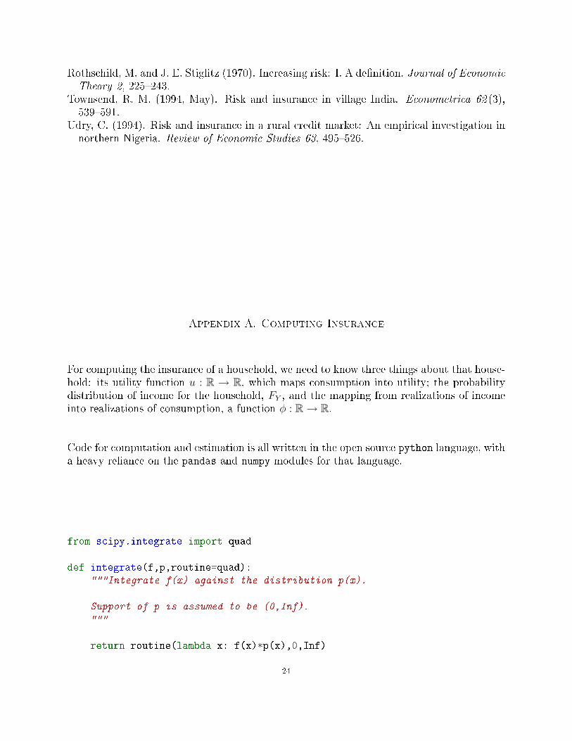
For computing the insurance of a household, we need to know three things about that house-hold: its utility function u : R → R, which maps consumption into utility; the probabilitydistribution of income for the household, FY , and the mapping from realizations of incomeinto realizations of consumption, a function φ : R→ R.
Code for computation and estimation is all written in the open source python language, witha heavy reliance on the pandas and numpy modules for that language.
from scipy.integrate import quad
def integrate(f,p,routine=quad):"""Integrate f(x) against the distribution p(x).
Support of p is assumed to be (0,Inf).
"""
return routine(lambda x: f(x)*p(x),0,Inf)
24

from pandas.io.pytables import HDFStorefrom pandas import DataFrame, Series
def ols(df,yname,Xnames):
mydf=DataFrame(df[[yname]+Xnames])
mydf.ix[~isfinite(mydf[yname]),yname]=NaN # Put infinite values to NaN...
for x in Xnames:try:
mydf.ix[~isfinite(mydf[x]),x]=NaNexcept TypeError: pass # E.g., ints can't be set to NaN.
mydf=mydf.dropna() # ...and then drop all rows with NaNs.
X=matrix(mydf[Xnames])y=matrix(mydf[yname]).T
b=linalg.lstsq(X,y)[0]
u=y-X*b
se=sqrt(diag(var(u)*(X.T*X).I))
d={'Coeff.':b.A.reshape((-1,)),'Std. Err.':se}
b=DataFrame(data=d,index=Xnames)
u=Series(data=u.A.reshape((-1,)),index=mydf.index,name='Residuals')
return b,u
The following code constructs a measure of aggregate income, and constructs de-meanedversions of log consumption and log income (all in per capita terms). The resulting datasetis meant to be suitable for analysis.
25

"""
Create dataset for analysis from IFLS data.
"""
from pandas.io.pytables import HDFStorefrom pandas import DataFramefrom pylab import *
store=HDFStore('IFLS/aggregate_inc.h5')otherstore=HDFStore('IFLS/ifls.h5')store2=HDFStore('IFLS/r1covar.h5') # Round 1 characteristics compiled by Diana Lee
hhchars=store2['/r1covar']hhchars['caseid']=hhchars['hhid93']hhchars.set_index('caseid',drop=False,inplace=True)
hhsize=otherstore['/hhsize']hhsize=hhsize.merge(hhchars,on='caseid')
hhsize['hhsize']=hhsize['hhsize_x']hhsize['hhsize93']=hhsize['hhsize_y']del hhsize['hhsize_x']del hhsize['hhsize_y']hhsize['round']=hhsize['round'].apply(lambda x:str(int(x)))hhsize.set_index(['caseid','round'],inplace=True,drop=False)hhsize.sort_index(inplace=True)
del hhsize['round']del hhsize['caseid']
S=store['/aggregate_inc']S['round']=S['round'].apply(lambda x:str(int(x)))
S.set_index(['caseid','round'],inplace=True,drop=False)
S.sort_index(inplace=True)
S=S.join(hhsize,on=['caseid','round'])
# Different sources of income are:
income_sources={'asset' : 'Asset income','business_inc' : 'Business income','income_oth_hh' : 'Other income','income_hh' : 'Labor earnings','transfer_all' : 'Transfer income'}
# If data for any income source missing, we assume it's zero:
income={}for src in income_sources.keys():
inc_src=S[src]/S['hhsize'] # Put each income source in per capita terms.
inc_src[isnan(inc_src)]=0.income[src]=inc_src
income=DataFrame(income)
# Construct aggregate income
income['all_income']=income['asset']+income['business_inc']+income['income_hh']+income['income_oth_hh']income['hhsize']=S['hhsize']
# Now build matrix for regression
analysis=income.copy()
# Define measure of log consumption (in per capita terms)
analysis['logc']=log(S['food_tot'])-log(S['hhsize'])
# Compute household specific mean incomes.
## Start by getting list of unique caseids.
analysis['mu']=0.analysis['alpha']=0.
for thiscase in analysis.index.levels[0]:mu=mean(log(analysis.ix[thiscase]['all_income']))analysis.ix[thiscase]['mu']=mu
alpha=mean((analysis.ix[thiscase]['logc']))analysis.ix[thiscase]['alpha']=alpha
analysis.ix[analysis['mu']<0,'mu']=NaN
analysis['log income shock']=log(analysis['all_income']) - analysis['mu']
# For households with just 1 round:
analysis.ix[analysis['log income shock']==0,'log income shock']=NaN
# For households with average annual income less than 1000 Rupiah (less than 0.50 1993 USD):
analysis.ix[analysis['mu']<0,'mu']=NaN
analysis['log consumption shock']=analysis['logc'] - analysis['alpha']analysis.ix[~isfinite(analysis['log consumption shock']),'log consumption shock']=NaN
# Build time effects
for r in range(1,5):analysis['r%d' % r]=0.analysis.ix[S['round']==str(r),'r%d' % r]=1.
# Add household characteristics
analysis['rural']=S['rural']analysis['Head age']=S['hhage']analysis['Head educ.']=S['hheduc']analysis['Female head']=S['hhfemale']analysis['Household size (1993)']=S['hhsize93']
new_store=HDFStore('ifls.h5')
new_store['/ifls_analysis']=analysisstore.close()otherstore.close()new_store.close()
26
from pandas.io.pytables import HDFStorefrom pandas import DataFramefrom pylab import *
store=HDFStore('../Data/ifls.h5')analysis=store['/ifls_analysis']
The following function simply compiles the several di�erent expected values required tocalculate the quantities we're interested in.
from numpy import log
def compile_expected_values(Ey,Ec,u=log):"""
Return (E(y), E(c), Eu(y), Eu(c), Eu(yL)).
Ey and Ec compute the expectation of a function with respect to
the distribution of y and c, respectively.
The argument u is a function mapping consumption into utility, which
defaults to the log function.
"""
X=[Ey(),Ec(),Ec(u)]X.append(Ey(lambda x:u(x*X[1]/X[0])))
return tuple(X)
The following code de�nes an expectation operator to computes expected values of an arbi-trary function f : R→ R with respect to an arbitrary distribution.
27

<<integrate>>import scipy.stats.distributions as distributionsfrom numpy import exp, Inffrom warnings import warn
def E(f,pdf,tol=1e-3):"""General expectations operator. Uses quadrature to integrate a function f against pdf.
"""
x,e=integrate(f,pdf)if abs(e)>tol:
warn("Integration error %g greater than tolerance %g" %(e,tol))
return x
# print abs(E(lambda x:x,dist(3,2))-exp(3+(2**2)/2.)) # Test
When income is distributed log-normal we can do better by specializing, and de�ning expec-tations with respect to the distribution of income by relying on features of that distribution.
import scipy.stats.distributions as distributions
Ey=lambda f=None,mu=0.,sigma=1. : distributions.lognorm.expect(f,sigma,scale=exp(mu))
With this, we can easily compute the expected value of functions of income; for example thefollowing code computes Eyβ:
<<expectation_y>>
from numpy import log, exp
mu=3.sigma=0.5beta=2./3
f=lambda y:y**beta
print Ey(f,mu,sigma)28
<<ifls>><<ols>>
analysis.ix[~isfinite(analysis['alpha']),'alpha']=NaNanalysis.ix[~isfinite(analysis['mu']),'mu']=NaN
use=analysis.dropna()n=len(use)
use['e2']=use['log income shock']**2use[r'$\mu_i$']=use['mu']use[r'$(\mu_i-\bar\mu)^2$']=(use['mu']-mean(use['mu']))**2use['Constant']=1.
b=ols(use,'e2',['Constant',r'$\mu_i$',r'$(\mu_i-\bar\mu)^2$'])[0]a=b['Coeff.']
use[r'$\sigma_i$']=sqrt(a[0]+a[1]*use[r'$\mu_i$']+a[2]*(use[r'$\mu_i$']-mean(use[r'$\mu_i$']))**2)
Now, the following function de�nes a Jalan-Ravallion consumption function, provided thatincome is the only random variable that a�ects consumption.
from numpy import exp
def phi_jr(mu,alpha,beta):"""Expected value of consumption with Jalan-Ravallion consumption function.
"""
phi = lambda y: exp(alpha-beta*mu)*y**beta
return phi
The consumption function phi_jr takes three parameters: µ, α, and β. The �rst two arejust household-speci�c means log income and consumption, respectively, which we've alreadycalculated. That leaves the quantity β, which we compute using the following code.
29
<<ifls>><<ols>>
analysis.ix[~isfinite(analysis['log consumption shock']),'log consumption shock']=NaNanalysis.ix[~isfinite(analysis['log income shock']),'log income shock']=NaN
use=analysis.dropna()n=len(use)
use['Constant']=1.b,u=ols(use,'log consumption shock',['Constant','log income shock'])
Now we're in a position to de�ne a function to compute expectations of functions with respectto the distribution of consumption:
def Ec(f=None,phi=lambda x:x,Ey=None):
if f==None:return Ey(phi)
else:return Ey(lambda x:f(phi(x)))
If unobservable random variables in�uence consumption instead of just income, then ex-pected consumption computed from a function such as Ec and phi_jr will be a lower bound.However, so long as these unobservables are distributed independently of y then we can com-pute their in�uence on the expected value of c simply by scaling up by a factor Eeε, whereε is the e�ect of the unobservable factors on log consumption.
If one knew the distribution of the ε one could of course integrate to calculate the expectedvalue Eeε. But we can also compute estimates of these unobservables from the same regres-sion we use to estimate β, simply by computing the sample mean of eε, where the ε are theresiduals. Since the mean of the residuals is zero, by Jensen's inequality the mean of theexponential must be non-negative, and allows us to simply scale up our estimate of the lowerbound of expected consumption to obtain an upper bound.
The distribution of income and consumption for a particular household i then depends on justa vector of parameters (αi, β, µi, σi,E exp ε). Note that we assume the values of (β,E exp ε)are common across households, though of course this could be easily changed.
30
<<expectation_y>><<expectation_c>><<phi_jr>>
def household_insurance(alpha,beta,mu,sigma,scaling=None,u=log):
phi=phi_jr(mu,alpha,beta)Eiy=lambda f=None:Ey(f,mu,sigma)Eic=lambda f=None:Ec(f,phi,Eiy)
identity=lambda x:xd={}
d['\E_s(c)']=Eic(identity)d['\E_s(u(c))']=Eic(u)d['\E_s(y)']=Eiy(identity)d['\E_s(u(y))']=Eiy(u)
d['L_s']=d['\E_s(c)']/d['\E_s(y)']d['\E_s(u(yL_s))']=Eiy(lambda y:u(y*d['L_s']))
d['I_s']=u(d['\E_s(y)'])-d['\E_s(u(y))']d['P_s']=d['\E_s(u(y))']-d['\E_s(u(yL_s))']d['A_s']=d['\E_s(u(c))']-d['\E_s(u(yL_s))']
if scaling:d['\E_s(c) (upper bound)']=d['\E_s(c)']*scaling
d['L_s (upper bound)']=d['\E_s(c) (upper bound)']/d['\E_s(y)']
d['\E_s(u(yL_s)) (upper bound)']=Eiy(lambda x:u(x*d['L_s (upper bound)']))
d['P_s (upper bound)']=d['\E_s(u(y))']-d['\E_s(u(yL_s)) (upper bound)']
return d
Appendix B. Data from the Indonesian Family Life Survey
There are currently four rounds of available data for the Indonesian Family Life Survey, from1993, 1997, 2000, and 2007. The sample sizes are given in Table 5. The data is longitudi-nal and follows both household and individuals within households, thus capturing any newhouseholds that may have formed in the interim period. A total of 15006 unique householdsappeared in the pooled sample. Of the 7216 households originally sampled in 1993, 6060 weresurveyed during all four rounds. Of the additional households which appeared in the latterrounds of the survey, 562 newly formed households went on to complete the last three waves
31
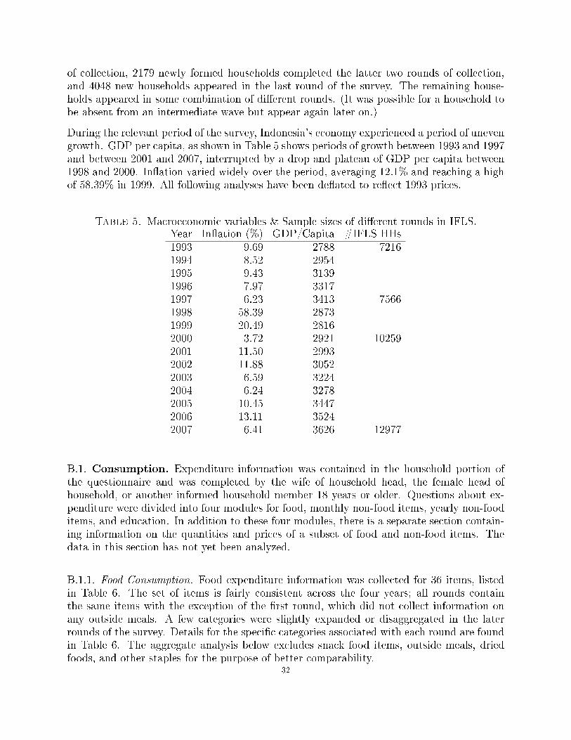
of collection, 2179 newly formed households completed the latter two rounds of collection,and 4048 new households appeared in the last round of the survey. The remaining house-holds appeared in some combination of di�erent rounds. (It was possible for a household tobe absent from an intermediate wave but appear again later on.)
During the relevant period of the survey, Indonesia's economy experienced a period of unevengrowth. GDP per capita, as shown in Table 5 shows periods of growth between 1993 and 1997and between 2001 and 2007, interrupted by a drop and plateau of GDP per capita between1998 and 2000. In�ation varied widely over the period, averaging 12.1% and reaching a highof 58.39% in 1999. All following analyses have been de�ated to re�ect 1993 prices.
Table 5. Macroeconomic variables & Sample sizes of di�erent rounds in IFLS.Year In�ation (%) GDP/Capita #IFLS HHs1993 9.69 2788 72161994 8.52 29541995 9.43 31391996 7.97 33171997 6.23 3413 75661998 58.39 28731999 20.49 28162000 3.72 2921 102592001 11.50 29932002 11.88 30522003 6.59 32242004 6.24 32782005 10.45 34472006 13.11 35242007 6.41 3626 12977
B.1. Consumption. Expenditure information was contained in the household portion ofthe questionnaire and was completed by the wife of household head, the female head ofhousehold, or another informed household member 18 years or older. Questions about ex-penditure were divided into four modules for food, monthly non-food items, yearly non-fooditems, and education. In addition to these four modules, there is a separate section contain-ing information on the quantities and prices of a subset of food and non-food items. Thedata in this section has not yet been analyzed.
B.1.1. Food Consumption. Food expenditure information was collected for 36 items, listedin Table 6. The set of items is fairly consistent across the four years; all rounds containthe same items with the exception of the �rst round, which did not collect information onany outside meals. A few categories were slightly expanded or disaggregated in the laterrounds of the survey. Details for the speci�c categories associated with each round are foundin Table 6. The aggregate analysis below excludes snack food items, outside meals, driedfoods, and other staples for the purpose of better comparability.
32
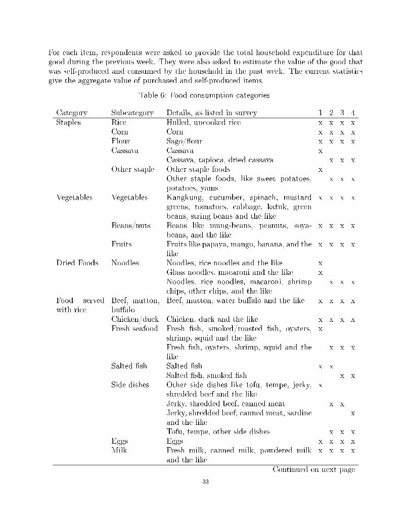
For each item, respondents were asked to provide the total household expenditure for thatgood during the previous week. They were also asked to estimate the value of the good thatwas self-produced and consumed by the household in the past week. The current statisticsgive the aggregate value of purchased and self-produced items.
Table 6: Food consumption categories
Category Subcategory Details, as listed in survey 1 2 3 4Staples Rice Hulled, uncooked rice x x x x
Corn Corn x x x xFlour Sago/�our x x x xCassava Cassava x
Cassava, tapioca, dried cassava x x xOther staple Other staple foods x
Other staple foods, like sweet potatoes,potatoes, yams
x x x
Vegetables Vegetables Kangkung, cucumber, spinach, mustardgreens, tomatoes, cabbage, katuk, greenbeans, string beans and the like
x x x x
Beans/nuts Beans like mung-beans, peanuts, soya-beans, and the like
x x x x
Fruits Fruits like papaya, mango, banana, and thelike
x x x x
Dried Foods Noodles Noodles, rice noodles and the like xGlass noodles, macaroni and the like xNoodles, rice noodles, macaroni, shrimpchips, other chips, and the like
x x x
Food servedwith rice
Beef, mutton,bu�alo
Beef, mutton, water bu�alo and the like x x x x
Chicken/duck Chicken, duck and the like x x x xFresh seafood Fresh �sh, smoked/roasted �sh, oysters,
shrimp, squid and the likex
Fresh �sh, oysters, shrimp, squid and thelike
x x x
Salted �sh Salted �sh x xSalted �sh, smoked �sh x x
Side dishes Other side dishes like tofu, tempe, jerky,shredded beef and the like
x
Jerky, shredded beef, canned meat x xJerky, shredded beef, canned meat, sardineand the like
x
Tofu, tempe, other side dishes x x xEggs Eggs x x x xMilk Fresh milk, canned milk, powdered milk
and the likex x x x
Continued on next page
33

Table 6: Food consumption categories
Category Subcategory Details, as listed in survey 1 2 3 4Spices Soy sauce Sweet and salty soy sauce x x x x
Salt Salt x x x xShrimp paste Shrimp paste x x x xChili/tomatosauce
Chili sauce, tomato sauce, and the like x x x x
Spices Shallot, garlic, chilic, candle nuts, corrian-der, MSG and the like
x x x x
Brown sugar Javanese (brown) sugar x x x xButter Butter x x x xOil Cooking oil like coconut oil, peanut oil,
corn oil, palm oil and the likex x x x
B.1.2. Non-food Expenditures. Together with the detailed food module, the modules onmonthly non-food items, yearly non-food items, and education provide a broader pictureof overall household expenditures. The items included in these modules are detailed in Ta-ble tab:non_foodcat and are classi�ed into six categories: household goods, living expenses,health, social expenditures, education, and other. As with the food module, the questionsasked are fairly consistent across surveys, though some of the items are more disaggregatedin the latter surveys. Irregular gifts (under the social category) were not included in the �rstround and excluded from the analysis. In addition, the �rst survey di�ered from the rest inthe relevant time period for educational expenses and some items in the other category.
Table 7: Non-food consumption categories
Category Subcategory Timeperiod
Details 1 2 3 4
Food Food Week Aggregated x x x xHouseholdgoods
Toiletries Month Personal toiletries including soap,shaving supplies, cosmetics and thelike
x x x x
Householditems
Month Household items including laun-dry soap, cleaning supplies, servantwages, telephone charges and thelike
x
Month Household items including laundrysoap, cleaning supplies and the like
x x
Month Household items including laun-dry soap, cleaning supplies, anti-mosquitoes and the like
x
Month Domestic services and servants'wages
x x x
Continued on next page
34

Table 7: Non-food consumption categories
Category Subcategory Timeperiod
Details 1 2 3 4
Clothes Year Clothing including shoes, hats,shirts, pants, children clothing andthe like
x x x
Supplies Year Household supplies and furnitureincluding tables, chairs, kitchentools, sheets, towels and the like
x
Year Household supplies and furnitureincluding beds, tables, chairs,kitchen tools, towels and the like
x
Year Household supplies and furnitureincluding tables, chairs, kitchentools, bed sheets, towels and thelike
x
Living ex-penses
Utilities Month Electricity, water, fuel and the like x x
Month Electricity, water, fuel, telephoneand the like
x
Month Electricity xMonth Water xMonth Fuel xMonth Telephone (including vouchers and
mobile starter pack)x
Recreation Month Recreation and entertainment in-cluding movies, theater, outings,sport equipment, magazines andthe like
x x x
Recreation Month Recreation and entertainment in-cluding movies, theater, outings,sport equipment, newspapers, mag-azines and the like
x
Transportation Month Transportation including bus far,cab fare, (vehicle) taxes and repaircosts, fuel and the like
x x x x
Taxes Year Taxes including property tax, in-come tax, sales tax and the like
x x x x
Health Medical Year Medical costs including hospitaliza-tion costs, clinic charges, physi-cian's fee, traditional healer's fee,medicines and the like
x x x x
Continued on next page
35

Table 7: Non-food consumption categories
Category Subcategory Timeperiod
Details 1 2 3 4
Social Regular gifts Month Value of non-food items given toothers/other parties outside thehousehold on a regular basis
x x x
Month Value of non-food items given toothers/other parties outside thehousehold on a regular basis (in-cluding debt repayment)
x
Ceremonies Year Ritual ceremonies, charities andgifts including weddings, circumci-sions, tithe, charities, gifts and thelike
x x x x
Irregular gifts Year Value of non-food items given toothers/other parties outside thehousehold on an irregular basis (lessthan one time per month)
x x x
Education Tuition Year Approximately what was the to-tal expenditures (e.g. tuition,PTA contribution, laboratory, reg-istration ,exams, other contributionlike student associations for chil-dren/family members both insideand outside the household
x x
Year Approximately what was the totalexpenditures (e.g. tuition, regis-tration fees, exams, other contri-bution like student associations forchildren/family members both in-side and outside the household
x
Month Approximately what was the to-tal monthly expenditures (tuition,pocket money) for children/familymembers both inside and outsidethe household
x
School needs Year Approximately what was the to-tal expenditures for schooling needs(like for school uniforms, schoolsupplies) for children/family mem-bers both inside and outside thehousehold
x x x
Continued on next page
36
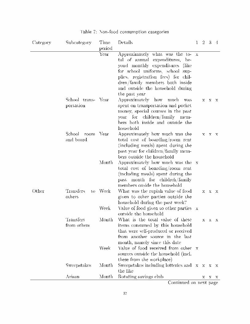
Table 7: Non-food consumption categories
Category Subcategory Timeperiod
Details 1 2 3 4
Year Approximately what was the to-tal of annual expenditures, be-yond monthly expenditures (likefor school uniforms, school sup-plies, registration fees) for chil-dren/family members both insideand outside the household duringthe past year
x
School trans-portation
Year Approximately how much wasspent on transportation and pocketmoney, special courses in the pastyear for children/family mem-bers both inside and outside thehousehold
x x x
School roomand board
Year Approximately how much was thetotal cost of boarding/room rent(including meals) spent during thepast year for children/family mem-bers outside the household
x x x
Month Approximately how much was thetotal cost of boarding/room rent(including meals) spent during thepast month for childreh/familymembers ouside the household
x
Other Transfers toothers
Week What was the rupiah value of foodgiven to other parties outside thehousehold during the past week?
x x x
Week Value of food given to other partiesoutside the household
x
Transfersfrom others
Month What is the total value of theseitems consumed by this householdthat were self-produced or receivedfrom another source in the lastmonth, namely since this date
x x x
Week Value of food received from othersources outside the household (incl.these from the workplace)
x
Sweepstakes Month Sweepstakes including lotteries andthe like
x x x x
Arisan Month Rotating savings club x x xContinued on next page
37

Table 7: Non-food consumption categories
Category Subcategory Timeperiod
Details 1 2 3 4
Other Year Other expenditures not speci�edabove including the purchase ofcars, television sets, beds, livestockand the like
x x x
Other' Year Other expenditures not speci�edabove including the purchase ofcars, house, television sets and thelike
x
B.2. Income.
B.2.1. General Notes. This documentation is for all households in all rounds. All values arefor thousands rupiah, de�ated to 1993 (de�ators=1.36, 2.69, and 5.06 for rounds 2, 3, and4, respectively). Individuals with data available from more than one survey (who appear inboth the adult and proxy surveys, or adult and female surveys) are given the maximum ofthe two values. No outliers are removed.
Aggregate household income is constructed as the sum of the yearly household income fromemployment, asset income, business income, and other income, and transfers from non-household members (analysis above leaves out transfer income). Data come from aggregatingacross the household economy and adult surveys.
There are two major issues with the income data. First, the adult surveys were not admin-istered to all adults in the household due to cost constraints. This provides a somewhatincomplete picture of total income. The fraction of adults surveyed is given below for therelevant sections. Second, due to aggregation over many di�erent variables, many householdsare missing aggregate household income. The details of construction and percent of missingvariables are given below by section.
38
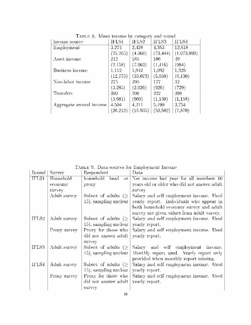
Table 8. Mean income by category and roundIncome source IFLS1 IFLS2 IFLS3 IFLS4Employment 3,274 2,428 4,353 12,818
(25,265) (4,368) (73,444) (1,073,899)Asset income 212 185 106 49
(2,158) (7,063) (1,416) (984)Business income 1,112 1,942 1,092 1,325
(12,775) (33,073) (5,938) (6,130)Non-labor income 275 295 177 32
(3,285) (2,026) (926) (729)Transfers 390 208 222 398
(3,981) (909) (1,130) (1,158)Aggregate annual income 4,504 4,211 5,190 3,754
(26,212) (15,935) (52,502) (7,870)
Table 9. Data sources for Employment IncomeRound Survey Respondent DataIFLS1 Household
economysurvey
household head orproxy
Net income last year for all members 10years old or older who did not answer adultsurvey
Adult survey Subset of adults (≥15), sampling unclear
Salary and self employment income. Usedyearly report. Individuals who appear inboth household economy survey and adultsurvey are given values from adult survey.
IFLS2 Adult survey Subset of adults (≥15), sampling unclear
Salary and self employment income. Usedyearly report.
Proxy survey Proxy for those whodid not answer adultsurvey
Salary and self employment income. Usedyearly report.
IFLS3 Adult survey Subset of adults (≥15), sampling unclear
Salary and self employment income.Monthly report used. Yearly report onlyprovided when monthly report missing.
IFLS4 Adult survey Subset of adults (≥15), sampling unclear
Salary and self employment income. Usedyearly report.
Proxy survey Proxy for those whodid not answer adultsurvey
Salary and self employment income. Usedyearly report.
39
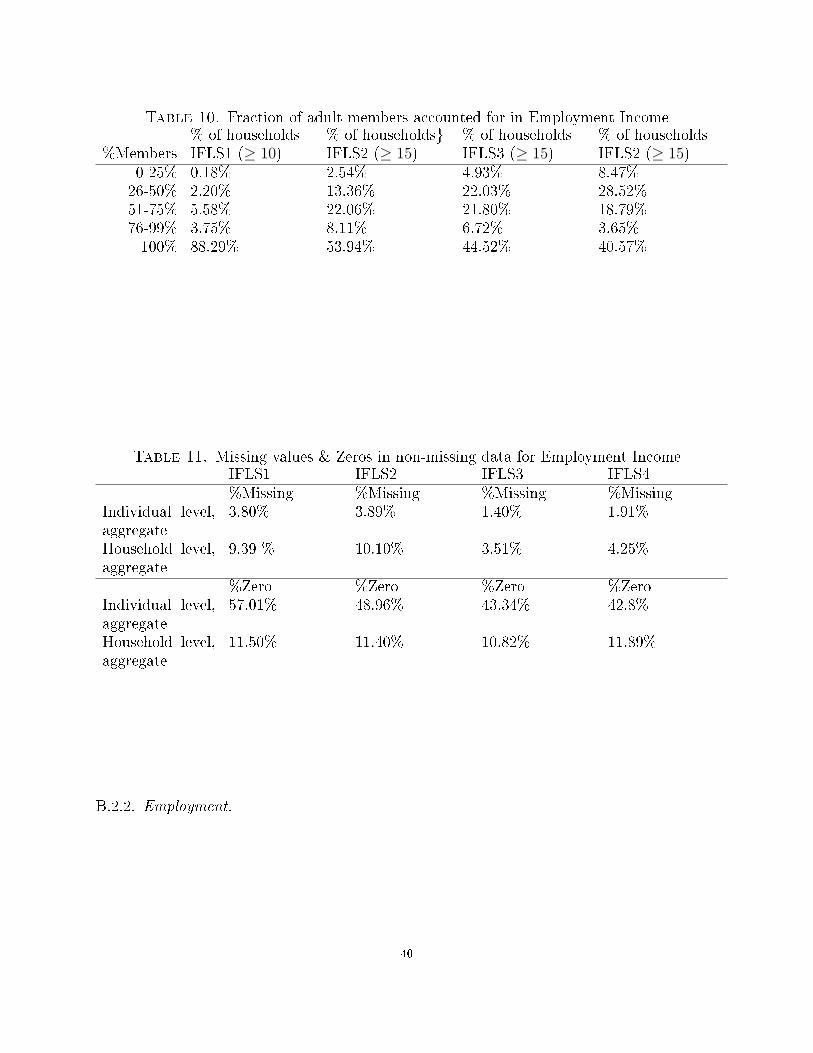
Table 10. Fraction of adult members accounted for in Employment Income% of households % of households} % of households % of households
%Members IFLS1 (≥ 10) IFLS2 (≥ 15) IFLS3 (≥ 15) IFLS2 (≥ 15)0-25% 0.18% 2.54% 4.93% 8.47%26-50% 2.20% 13.36% 22.03% 28.52%51-75% 5.58% 22.06% 21.80% 18.79%76-99% 3.75% 8.11% 6.72% 3.65%100% 88.29% 53.94% 44.52% 40.57%
Table 11. Missing values & Zeros in non-missing data for Employment IncomeIFLS1 IFLS2 IFLS3 IFLS4%Missing %Missing %Missing %Missing
Individual level,aggregate
3.80% 3.89% 1.40% 1.91%
Household level,aggregate
9.39 % 10.10% 3.51% 4.25%
%Zero %Zero %Zero %ZeroIndividual level,aggregate
57.01% 48.96% 43.34% 42.8%
Household level,aggregate
11.50% 11.40% 10.82% 11.89%
B.2.2. Employment.
40
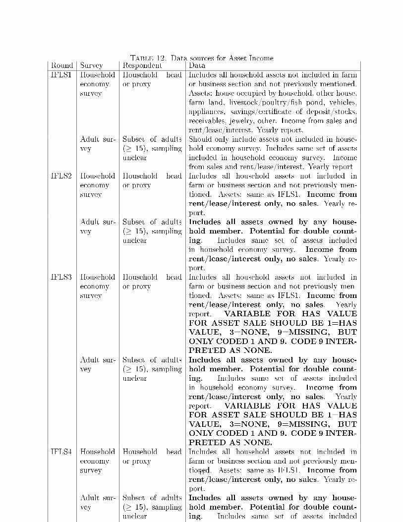
Table 12. Data sources for Asset IncomeRound Survey Respondent DataIFLS1 Household
economysurvey
Household heador proxy
Includes all household assets not included in farmor business section and not previously mentioned.Assets: house occupied by household, other house,farm land, livestock/poultry/�sh pond, vehicles,appliances, savings/certi�cate of deposit/stocks,receivables, jewelry, other. Income from sales andrent/lease/interest. Yearly report.
Adult sur-vey
Subset of adults(≥ 15), samplingunclear
Should only include assets not included in house-hold economy survey. Includes same set of assetsincluded in household economy survey. Incomefrom sales and rent/lease/interest. Yearly report
IFLS2 Householdeconomysurvey
Household heador proxy
Includes all household assets not included infarm or business section and not previously men-tioned. Assets: same as IFLS1. Income fromrent/lease/interest only, no sales. Yearly re-port.
Adult sur-vey
Subset of adults(≥ 15), samplingunclear
Includes all assets owned by any house-hold member. Potential for double count-ing. Includes same set of assets includedin household economy survey. Income fromrent/lease/interest only, no sales. Yearly re-port.
IFLS3 Householdeconomysurvey
Household heador proxy
Includes all household assets not included infarm or business section and not previously men-tioned. Assets: same as IFLS1. Income fromrent/lease/interest only, no sales. Yearlyreport. VARIABLE FOR HAS VALUEFOR ASSET SALE SHOULD BE 1=HASVALUE, 3=NONE, 9=MISSING, BUTONLY CODED 1 AND 9. CODE 9 INTER-PRETED AS NONE.
Adult sur-vey
Subset of adults(≥ 15), samplingunclear
Includes all assets owned by any house-hold member. Potential for double count-ing. Includes same set of assets includedin household economy survey. Income fromrent/lease/interest only, no sales. Yearlyreport. VARIABLE FOR HAS VALUEFOR ASSET SALE SHOULD BE 1=HASVALUE, 3=NONE, 9=MISSING, BUTONLY CODED 1 AND 9. CODE 9 INTER-PRETED AS NONE.
IFLS4 Householdeconomysurvey
Household heador proxy
Includes all household assets not included infarm or business section and not previously men-tioned. Assets: same as IFLS1. Income fromrent/lease/interest only, no sales. Yearly re-port.
Adult sur-vey
Subset of adults(≥ 15), samplingunclear
Includes all assets owned by any house-hold member. Potential for double count-ing. Includes same set of assets includedin household economy survey. Income fromrent/lease/interest only, no sales. Yearly re-port.
41

Table 13. Fraction of adult members (≥ 15) accounted for in adult surveyfor Asset Income.
%Members IFLS1 IFLS2 IFLS3 IFLS4Acctd. % of households % of households % of households % of households0-25% 8.18% 13.07% 17.54% 21.81%26-50% 30.29% 39.48% 38.37% 35.83%51-75% 16.70% 18.79% 14.34$ 10.54%76-99% 0.31% 1.32% 1.15% 0.83%100% 44.53% 27.34% 28.61% 30.99%
Table 14. Missing values & Zeros in non-missing data for Asset IncomeIFLS1 IFLS2 IFLS3 IFLS4
Survey %Missing %Missing %Missing %MissingIndividual level, adult survey 8.62% 6.99% 0.09% 8.12%Household level, adult survey 7.19 % 5.95% 0.08% 6.27%Household level, household econ-omy survey
11.53% 7.32% 0.07% 10.23%
Household level, aggregate 15.51% 11.20% 0.19% 13.08%%Zero %Zero %Zero %Zero
Individual level, adult survey 85.58% 94.33% 92.63% 96.11%Household level, adult survey 87.77% 95.31% 93.93% 97.22%Household level, household econ-omy survey
80.15% 93.38% 92.52% 95.66%
Household level, aggregate 76.56% 91.69% 89.57% 94.80%
B.2.3. Asset income.
42
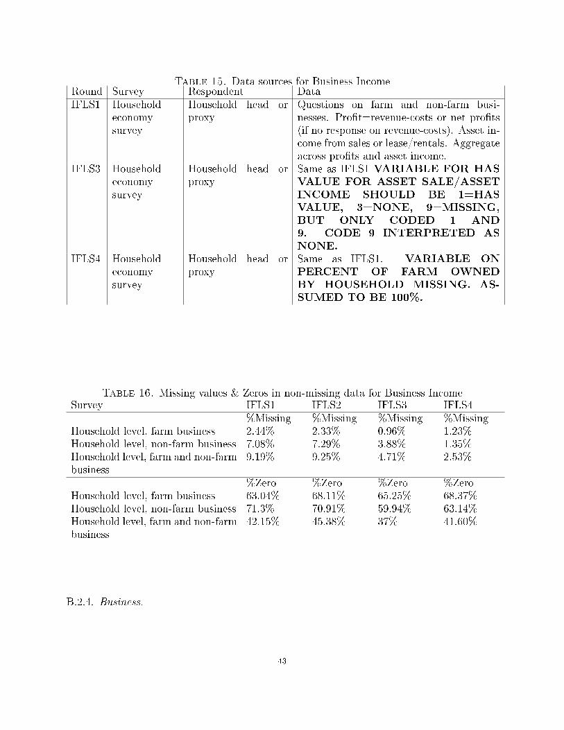
Table 15. Data sources for Business IncomeRound Survey Respondent DataIFLS1 Household
economysurvey
Household head orproxy
Questions on farm and non-farm busi-nesses. Pro�t=revenue-costs or net pro�ts(if no response on revenue-costs). Asset in-come from sales or lease/rentals. Aggregateacross pro�ts and asset income.
IFLS3 Householdeconomysurvey
Household head orproxy
Same as IFLS1 VARIABLE FOR HASVALUE FOR ASSET SALE/ASSETINCOME SHOULD BE 1=HASVALUE, 3=NONE, 9=MISSING,BUT ONLY CODED 1 AND9. CODE 9 INTERPRETED ASNONE.
IFLS4 Householdeconomysurvey
Household head orproxy
Same as IFLS1. VARIABLE ONPERCENT OF FARM OWNEDBY HOUSEHOLD MISSING. AS-SUMED TO BE 100%.
Table 16. Missing values & Zeros in non-missing data for Business IncomeSurvey IFLS1 IFLS2 IFLS3 IFLS4
%Missing %Missing %Missing %MissingHousehold level, farm business 2.44% 2.33% 0.96% 1.23%Household level, non-farm business 7.08% 7.29% 3.88% 1.35%Household level, farm and non-farmbusiness
9.19% 9.25% 4.71% 2.53%
%Zero %Zero %Zero %ZeroHousehold level, farm business 63.04% 68.11% 65.25% 68.37%Household level, non-farm business 71.3% 70.91% 59.94% 63.14%Household level, farm and non-farmbusiness
42.15% 45.38% 37% 41.60%
B.2.4. Business.
43
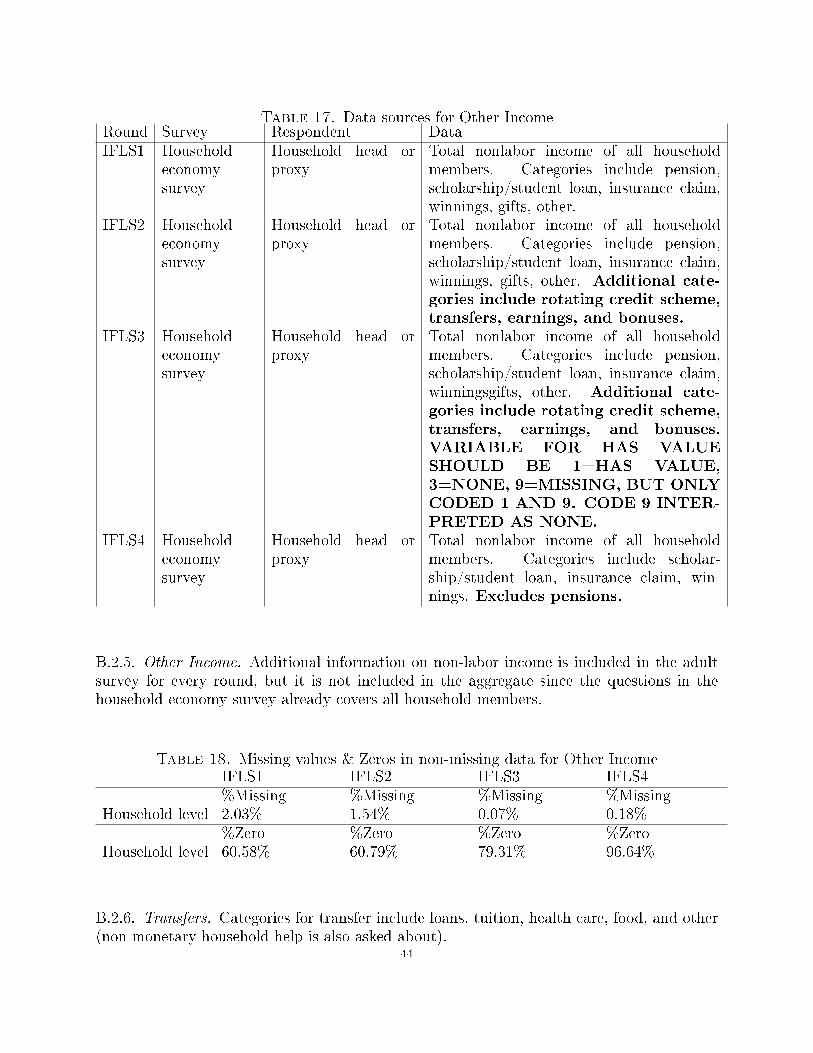
Table 17. Data sources for Other IncomeRound Survey Respondent DataIFLS1 Household
economysurvey
Household head orproxy
Total nonlabor income of all householdmembers. Categories include pension,scholarship/student loan, insurance claim,winnings, gifts, other.
IFLS2 Householdeconomysurvey
Household head orproxy
Total nonlabor income of all householdmembers. Categories include pension,scholarship/student loan, insurance claim,winnings, gifts, other. Additional cate-gories include rotating credit scheme,transfers, earnings, and bonuses.
IFLS3 Householdeconomysurvey
Household head orproxy
Total nonlabor income of all householdmembers. Categories include pension,scholarship/student loan, insurance claim,winningsgifts, other. Additional cate-gories include rotating credit scheme,transfers, earnings, and bonuses.VARIABLE FOR HAS VALUESHOULD BE 1=HAS VALUE,3=NONE, 9=MISSING, BUT ONLYCODED 1 AND 9. CODE 9 INTER-PRETED AS NONE.
IFLS4 Householdeconomysurvey
Household head orproxy
Total nonlabor income of all householdmembers. Categories include scholar-ship/student loan, insurance claim, win-nings. Excludes pensions.
B.2.5. Other Income. Additional information on non-labor income is included in the adultsurvey for every round, but it is not included in the aggregate since the questions in thehousehold economy survey already covers all household members.
Table 18. Missing values & Zeros in non-missing data for Other IncomeIFLS1 IFLS2 IFLS3 IFLS4%Missing %Missing %Missing %Missing
Household level 2.03% 1.54% 0.07% 0.18%%Zero %Zero %Zero %Zero
Household level 60.58% 60.79% 79.31% 96.64%
B.2.6. Transfers. Categories for transfer include loans, tuition, health care, food, and other(non-monetary household help is also asked about).
44

Table 19. Data sources for Transfers from non-coresident parents and siblingsRound Survey Respondent DataIFLS1 Adult
survey,sectionBA
head of house-hold, wife of headof household,selected seniorhousehold andspoue
Parent: asked for parents who do not live in house-hold and are alive/died within the past year. Sib-ling: asked for siblings who do not live in house-hold and are ≥ 15 years old and are alive/diedwithin the past year, detailed questions are askedabout a selected subsample of older siblings, trans-fers from non-selected subsample obtained fromsingle question.
Adult sur-vey, trans-fer section
adult respondentswho did not re-spond o BA
Parent: asked for parents who do not live in house-hold and are alive/died within the past year. Sib-lings: total transfer from all noncoresident siblingsobtained from single question.
IFLS2 Adult sur-vey
subset of adults≥15
Parent: asked for parents who do not live in house-hold and are alive/died within the past year. Sib-lings: total transfer from all noncoresident siblingsobtained from single question.
Proxy sur-vey
proxy for thosewho did not an-swer adult survey
Parent: asked for parents who do not live in house-hold and are alive/died within the past year. Sib-lings: total transfer from all noncoresident siblingsobtained from single question.
IFLS3 Adult sur-vey
subset of adults≥15
Parent: asked for parents who do not live inhousehold and are alive/died within the past year.No variable for which categories received.Summed over all non-missing categories.Siblings: total transfer from all noncoresident sib-lings obtained from single question.
Proxy sur-vey
proxy for thosewho did not an-swer adult survey
Parent: asked for parents who do not live inhousehold and are alive/died within the past year.No variable for which categories received.Summed over all non-missing categories.Siblings: total transfer from all noncoresident sib-lings obtained from single question.
IFLS4 Adult sur-vey
subset of adults≥15
Parent: asked for parents who do not live in house-hold and are alive/died within the past year. Sib-lings: total transfer from all noncoresident siblingsobtained from single question.
Proxy sur-vey
proxy for thosewho did not an-swer adult survey
Parent: asked for parents who do not live in house-hold and are alive/died within the past year. Sib-lings: total transfer from all noncoresident siblingsobtained from single question.
45

Table 20. Data sources for Transfers from non-coresident childrenRound Survey Respondent DataIFLS1 Adult
survey,sectionBA
head of house-hold, wife of headof household,selected seniorhousehold andspoue
Children: asked for children who do not livein household and are ≥ 15 years old and arealive/died within the past year, detailed questionsare asked about a selected subsample of older chil-dren, transfers from non-selected subsample ob-tained from single question.
Adult sur-vey, trans-fer section
adult respondentswho did not re-spond to BA
Children: total transfer from all non-coresidentchildren obtained from single question.
Proxy sur-vey
proxy for thosewho did not an-swer adult survey
Children: transfer from each non-coresident child≥ 15
Femalesurvey
ever-marriedwomen aged15-49
Children: transfer from each non-coresident child.Biological and adopted children. ≥ 15
Proxy sur-vey
proxy for thosewho did not an-swer adult survey
Children: transfer from each non-coresident child≥ 15
Femalesurvey
ever-marriedwomen aged15-49
Children: transfer from each non-coresident child.Biological and adopted children. ≥ 15 MUL-TIPLE LINES PER INDIVIDUAL. NOTCLEAR WHY. SUM OVER INDIVIDU-ALS. NOT MISSING UNLESS ALL LINESMISSING.
Proxy sur-vey
proxy for thosewho did not an-swer adult survey
Children: transfer from each non-coresident child≥ 15. MULTIPLE LINES PER INDIVID-UAL. NOT CLEAR WHY. SUM OVERINDIVIDUALS. NOT MISSING UNLESSALL LINES MISSING.
46
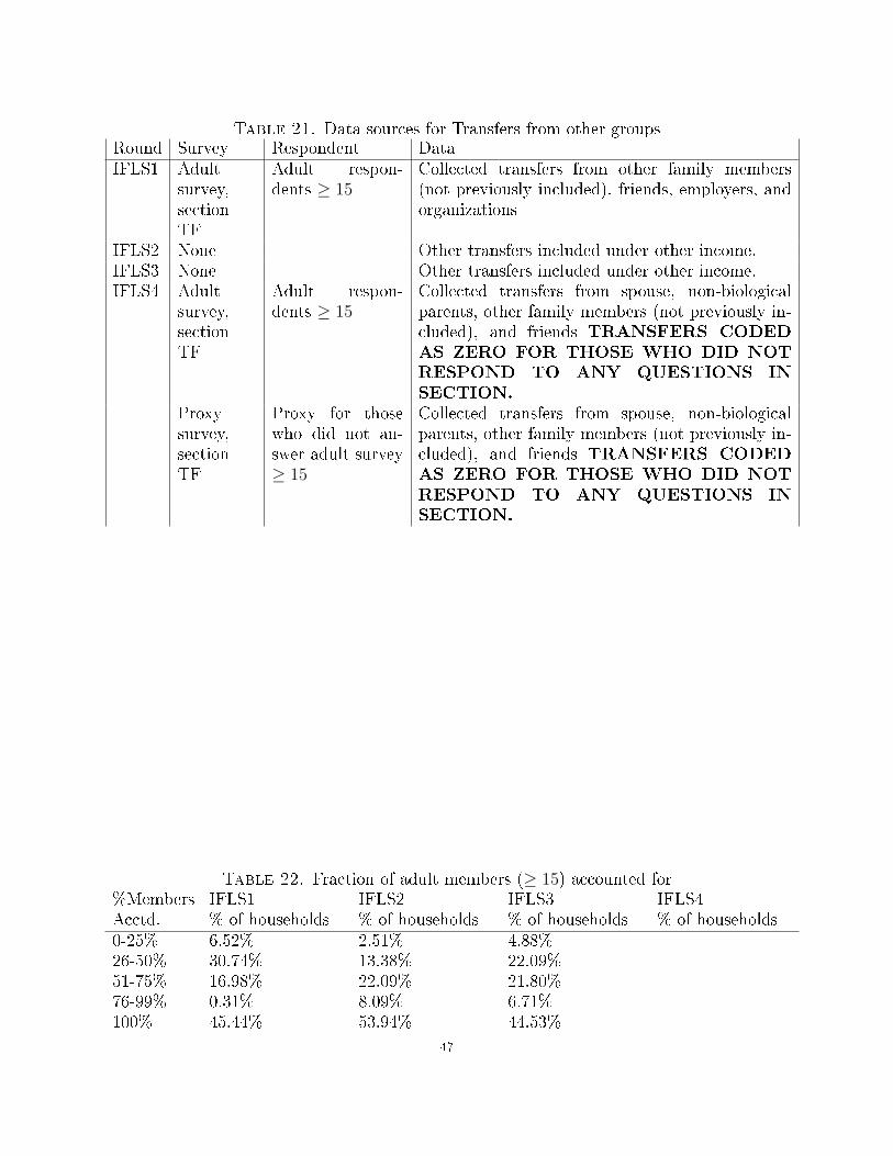
Table 21. Data sources for Transfers from other groupsRound Survey Respondent DataIFLS1 Adult
survey,sectionTF
Adult respon-dents ≥ 15
Collected transfers from other family members(not previously included), friends, employers, andorganizations
IFLS2 None Other transfers included under other income.IFLS3 None Other transfers included under other income.IFLS4 Adult
survey,sectionTF
Adult respon-dents ≥ 15
Collected transfers from spouse, non-biologicalparents, other family members (not previously in-cluded), and friends TRANSFERS CODEDAS ZERO FOR THOSE WHO DID NOTRESPOND TO ANY QUESTIONS INSECTION.
Proxysurvey,sectionTF
Proxy for thosewho did not an-swer adult survey≥ 15
Collected transfers from spouse, non-biologicalparents, other family members (not previously in-cluded), and friends TRANSFERS CODEDAS ZERO FOR THOSE WHO DID NOTRESPOND TO ANY QUESTIONS INSECTION.
Table 22. Fraction of adult members (≥ 15) accounted for%Members IFLS1 IFLS2 IFLS3 IFLS4Acctd. % of households % of households % of households % of households0-25% 6.52% 2.51% 4.88%26-50% 30.74% 13.38% 22.09%51-75% 16.98% 22.09% 21.80%76-99% 0.31% 8.09% 6.71%100% 45.44% 53.94% 44.53%
47

Table 23. Missing values & Zeros in non-missing data for Transfer IncomeIFLS1 IFLS2 IFLS3 IFLS4%Missing %Missing %Missing %Missing
Household level, parental transfers 3.04% 6.49% 0.38% 1.49%Household level, sibling transfers 7.87% 8.30% 2.87% 3.15%Household level, child transfers 5.62% 4.44% 11.15% 10.15%Household level, other transfer 5.04% NA NA 1.42%Household level, aggregatetransfers
15.68% 14.61% 13.58% 14.17%
%Zero %Zero %Zero %ZeroHousehold level, parental transfers 78.75% 64.81% 55.11% 52.49%Household level, sibling transfers 65.04% 45.23% 40.29% 39.84%Household level, child transfers 77.42% 77.04% 86.97% 78.57%Household level, other transfers 69.48% NA NA 50.78%Household level, aggregatetransfers
36.49% 26.42% 22.15% 13.89%
48