risk analytics autumn 2018 - university of...
TRANSCRIPT


Contents
Introduction
1 Univariate statistics
2 Multivariate statistics
3 Modelling the market
4 Estimating market invariants
5 Evaluating allocations
6 Optimising allocations
7 Estimating market invariants with estimation risk
8 Evaluating allocations with estimation risk
9 Optimising allocations with estimation risk
10 Regulatory framework of risk management
2 / 229

Introduction
Introduction
financial assets are held out of an interest in their future payoffsfuture payoffs are riskyhence, asset management necessarily involves risk managementthe job market highly values risk management abilities
01.10.15 19.09.16 25.09.17 21.09.18risk jobs 665 512 566 554
total jobs 1,257 924 1,062 1,090
Table: ‘Quantitative finance’ searches on http://www.indeed.com
Risk managers are in great demand as a result of the troubles the banks havefound themselves in (Richard Lipstein, Boyden Global Executive Search)
Banks are failing to implement bonus plans that rein in the types of risksblamed for contributing to the financial crisis, [the Basel Committee on Bank-ing Supervision] said. Bank Bonus Plans Fail to Curb Financial Risks, Regu-lators Say (Bloomberg, 15 Oct 2010)
3 / 229

Introduction Caveat mercator
Our (ahem!) promise to youAny graduate of G53 Risk Analytics should be able to beat an index fundover the course of a market cycle.
a 2015 analysis in the FT of the difficulties of delivering consistentoutperformanceanother cautionary 2015 FT article2017: Warren Buffett’s $1mn bet that the S&P500 would outperforma portfolio of hedge funds selected by fund manager Ted Seidesclassic statements in favour of passive investment: Malkiel (2016)(too long, but up to date) v Malkiel (2003) (dated, but concise)
slides from a talk by John Cochrane on hedge fundsCochrane (2013) addressed a consequence of these results: should wejust conclude that “people are stupid”?
Bookstaber (2007) provides a compelling account of smart, talented,hard-working people losing vast quantities of moneyare G53 techniques the opposite of the ‘value’ techniques used byinvestors like Ben Graham and Warren Buffett (Schroeder, 2009), oran augmentation of them? 5 / 229

Introduction Caveat mercator
A little Learning is a dang’rous ThingIf “active” and “passive” management styles are defined in sensible ways,it must be the case that
1 before costs, the return on the average actively managed dollarwill equal the return on the average passively managed dollar and
2 after costs, the return on the average actively managed dollar willbe less than the return on the average passively managed dollar
These assertions will hold for any time period. Moreover, they dependonly on the laws of addition, subtraction, multiplication and division.Nothing else is required. (Sharpe, 1991)
market return: “weighted average of the returns on the active andpassive segments of the market”average passive return: same as the market returnhence average active return is tooactive management faces higher costs
6 / 229
Introduction A standard risk taxonomy
Market risk
The best known type of risk is probably market risk: the risk of achange in the value of a financial position due to changes in thevalue of the underlying components on which that portfolio de-pends, such as stock and bond prices, exchange rates, commodityprices, etc. (McNeil, Frey and Embrechts, 2015, p.5)
Resti and Sironi (2007, Part II)
8 / 229
Introduction A standard risk taxonomy
Credit riskThe next important category is credit risk: the risk of not receivingpromised repayments on outstanding investments such as loansand bonds, because of the “default” of the borrower. (McNeil,Frey and Embrechts, 2015, p.5)
reflects, more generally, “unexpected changes in the creditworthinessof [a bank’s] counterparties” (Resti and Sironi, 2007, Part III); theyfeel it to be the most important classsee also Gordy (2000) or Bielecki and Rutkowski (2002)
Freddie Mac could incur “billions of dollars of losses” for US taxpayersby focussing on mortgages failing in the first two years; while,historically, this is when most have failed, more recent ‘teaser’mortgages have low interest rates for three to five years, which thenrise sharply (Freddie Mac Loan Deal Defective, Report Says, NYT, 27Sept 2011)
9 / 229
Introduction A standard risk taxonomy
Operational risk
A further risk category is operational risk: the risk of losses res-ulting from inadequate or failed internal processes, people andsystems, or from external events. (McNeil, Frey and Embrechts,2015, p.5)
Resti and Sironi (2007, Part IV)
The loss resulted from unauthorised speculative trading in variousS&P 500, Dax and Eurostoxx index futures over the past threemonths. The positions had been offset in our systems with ficti-tious, forward-settling, cash ETF positions, allegedly executed bythe trader. These fictitious trades concealed the fact that the in-dex futures trades violated UBS’s risk limits. (UBS, 18 September2011)
10 / 229

Introduction A standard risk taxonomy
Model risk
Model risk management has become a board-level process. Nowthe chief risk officer has to go to the board and not only talkabout market risk, credit risk and operational risk, he also has totalk about model risk. It is a huge organisational change. (NewYork-based model risk manager; Sherif (2016))
arises from a misspecified modele.g. using Black-Scholes when model assumptions don’t hold (e.g.normally distributed returns)“always present to some degree” (McNeil, Frey and Embrechts, 2015,p.5)q.v. Rebonato (2007), Supervisory Guidance on model riskmanagement (2011), Morini (2011)
11 / 229

Introduction A standard risk taxonomy
Liquidity risk
When we talk about liquidity risk we are generally referring toprice or market liquidity risk, which can be broadly defined as therisk stemming from the lack of marketability of an investment thatcannot be bought or sold quickly enough to prevent or minimizea loss. (McNeil, Frey and Embrechts, 2015, p.5)
In banking, there is also the concept of funding liquidity risk, whichrefers to the easer with which institutions can raise funding tomake payments and meet withdrawals as they arise. (McNeil,Frey and Embrechts, 2015, p.5)
12 / 229
Introduction The Meucci mantra
The Meucci mantra
1 for each security, identify the iid stochastic terms (§3.1)2 estimate the distribution of the market invariants (§4)3 project the invariants to the investment horizon (§3.2)4 dimension reduce to make the problem more tractable (§3.4)5 evaluate the portfolio performance at the investment horizon (§5)
what is your objective function?6 pick the portfolio that optimises your objective function (§6)7 account for estimation risk
1 replace point parameter estimates with Bayesian distributions (§7)2 re-evaluate the portfolio distributions in this light (§8)3 robustly re-optimise (§9)
Observation shows that some statistical frequencies are, withinnarrower or wider limits, stable. But stable frequencies are not verycommon, and cannot be assumed lightly. Keynes (1921, p.381)
14 / 229
Introduction The Meucci mantra
Notational conventions
τ , investment horizonT , time at which the allocation decision is made
thus, T + τ is when the investments are to be evaluatedPt , the vector of prices at time tXt , a random variable that will realise at time txt , a realisation of the random variableiT ≡ x1, . . . , xT, a dataset of observed realisations
15 / 229
Univariate statistics Random variables and their representation
Random variables
a number whose realisation is, as yet, unknownits distribution may be known
a space of events, Ea probability distribution, P
a function from the space of events to the real linethus, x = X (e) for some event e in E
the probability of an event giving rise to a realised x ∈ [x , x ]:
P X ∈ [x , x ] ≡ P e ∈ E s.t. X (e) ∈ [x , x ] .
reads: the probability that random variable X takes on a value in[x , x ] is the probability of the set of events yielding a realised value ofthe random variable . . .going forward, typically suppress dependence on e, refer just to X
naïve statement
17 / 229

Univariate statistics Random variables and their representation
Probability density function (PDF), fX
1 the probability that the rv Xtakes on a value within a giveninterval
P X ∈ [x , x ] ≡∫ x
xfX (x) dx
2 why do the following also hold?
fX (x) ≥ 0∫ ∞
−∞fX (x) dx = 1
Example
fX (x) = 1√π
e−x2
−3 −2 −1 0 1 2 3
0.0
0.1
0.2
0.3
0.4
x
y
18 / 229

Univariate statistics Random variables and their representation
Cumulative distribution function (CDF), FX
1 the probability that the rv Xtakes on a value less than x
FX (x) ≡ P X ≤ x
=
∫ x
−∞fX (u) du
2 why do the following also hold?
FX (−∞) = 0FX (∞) = 1
FX non-decreasing
Example
FX (x) = 12 [1 + erf (x)]
where erf is the error function
erf (x) ≡ 2√π
∫ x
0e−t2dt
19 / 229

Univariate statistics Random variables and their representation
Characteristic function (cf), ϕX
1
ϕX (ω) ≡ E
eiωX, ω ∈ R
2 its properties are less intuitive(Meucci, 2005, q.v. pp.6-7)
3 particularly useful for handling(weighted) sums of independentrvs
Example
ϕX (ω) = e−12ω
2
−3 −2 −1 0 1 2 3
0.0
0.2
0.4
0.6
0.8
1.0
omega
phi
20 / 229
Univariate statistics Random variables and their representation
Quantile, QX
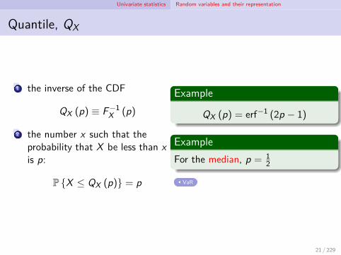
1 the inverse of the CDF
QX (p) ≡ F−1X (p)
2 the number x such that theprobability that X be less than xis p:
P X ≤ QX (p) = p
Example
QX (p) = erf−1 (2p − 1)
ExampleFor the median, p = 1
2
VaR
21 / 229
Univariate statistics Random variables and their representation
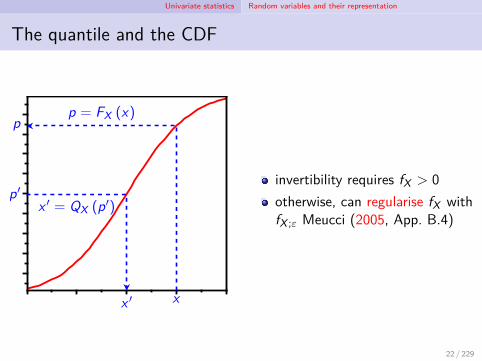
The quantile and the CDF
x
p = FX (x)p
p′x ′ = QX (p′)
x ′
invertibility requires fX > 0otherwise, can regularise fX withfX ;ε Meucci (2005, App. B.4)
22 / 229

Univariate statistics Random variables and their representation
Moving between representations of the rv X
QXinverses FX
D
fX
II F−1
F D
ϕX F−1
F
I is the integration operatorD is the derivative operatorF is the Fourier transform (FT)F−1 is the inverse Fourier transform(IFT)all of these are examples of linearoperators, A [v ] (x)
A, the linear operatorv , the function to which it is appliedx, the function’s argument
q.v. Meucci, Appendix B.3(n.b. fX exists iff FX is absolutelycontinuous; ϕX always exists)
23 / 229

Univariate statistics Random variables and their representation
Lecture 1 exercises
Meucci exercisespencil-and-paper: 1.1.1; 1.1.2; 1.1.3; 1.1.5; 1.1.6Python: 1.1.4, 1.1.7, 1.1.8
projectpick five assets for your project, ensuring that no one else is usingthem. Begin to experiment with your Interactive Brokers tradingaccount and the Bloomberg terminals.
24 / 229

Univariate statistics Summary statistics
Key summary parameters
full distributions can be expensive to representwhat summary information helps capture key features?
1 location, Loc Xif had one guess as to where X would take its valueshould satisfy Loc a = a and affine equivariance
Loc a + bX = a + bLoc X
to ensure independence of measurement scale/coordinate system2 dispersion, Dis X
how accurate the location guess, above, isaffine equivariance is now
Dis a + bX = |b|Dis X
where |·| denotes absolute value3 z-score normalises a rv, ZX ≡ X−LocX
DisX : 0 location; 1 dispersionaffine equivariance of location & dispersion ⇔ (Za+bX )
2 = (ZX )2
26 / 229

Univariate statistics Summary statistics
Most common location and dispersion measures‘local’ ‘semi-local’ ‘global’
location mode, Mod X median, Med X mean / exp’d val, E Xargmaxx∈R fX (x)
∫MedX−∞ fX (x) dx = 1
2∫∞−∞ xfX (x) dx
dispersion modal dispersion interquantile range variance∫∞−∞ (x − E X)2 fX (x) dx
‘global’ measures are formed from the whole distribution‘semi-local’ measures are formed from half (or so) of the distribution‘local’ measures are driven by individual observationsgenerally, we define
Dis X ≡ ∥X − Loc X ∥X ;p
where ∥g∥X ;p ≡ (E |g (X )|p)1p is the norm on the vector space Lp
Xp = 1 is the mean absolute deviation, MAD X ≡ E |X − E X|
p = 2 is the standard deviation, Sd X ≡(
E|X − E X|2
) 12
27 / 229
Univariate statistics Summary statistics
Higher order moments
1 kth-raw momentRMX
k ≡ E
X k
is the expectation of the kth power of X2 kth-central moment is more commonly used
CMXk ≡ E
(X − E X)k
de-means the raw moment, making it location-independent
skewness, a measure of symmetry, is the normalised 3rd central moment
Sk X ≡ CMX3
(Sd X)3
kurtosis measures the weights of the distribution’s tail relative to itscentre
Ku X ≡ CMX4
(Sd X)4
28 / 229
Univariate statistics Taxonomy of distributions
Uniform distribution: X ∼ U ([a, b])
simplest distribution; shall be useful when modelling copulasfully described by two parameters, a (lower bound) and b (upperbound)any outcome in the [a, b] is equally likelyclosed form representations for f U
a,b (x) ,F Ua,b (x) , ϕU
a,b (ω) and QUa,b (p)
standard uniform distribution is U ([0, 1])
30 / 229
Univariate statistics Taxonomy of distributions
Normal (Gaussian) distribution: X ∼ N(µ, σ2)
most widely used, studied distributionfully described by two parameters, µ (mean) and σ2 (variance)standard normal distribution when µ = 0 and σ2 = 1as a stable distribution, the sums of normally distributed rv’s arenormalclosed form representations for f N
µ,σ2 (x) ,F Nµ,σ2 (x) , ϕN
µ,σ2 (ω) andQNµ,σ2 (p)
why do we care that Ku X = 3?
31 / 229

Univariate statistics Taxonomy of distributions
Cauchy distribution: X ∼ Ca(µ, σ2)
‘fat-tailed’ distribution: when might this be useful?fully described by two parameters, µ and σ2
f Caµ,σ2 (x) ≡
1π√σ2
[1 +
(x − µ)2
σ2
]−1
what are E X ,Var X , Sk X and Ku X?see here for a discussion
standard Cauchy distribution when µ = 0 and σ2 = 1(FYI: if X ,Y ∼ NID (0, 1) then X
Y ∼ Ca (0, 1))
32 / 229
Univariate statistics Taxonomy of distributions
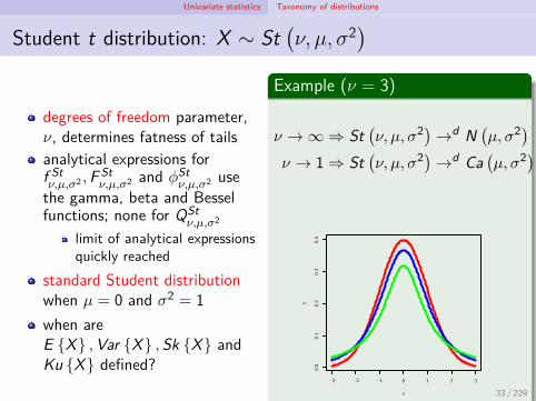
Student t distribution: X ∼ St(ν, µ, σ2)
degrees of freedom parameter,ν, determines fatness of tailsanalytical expressions forf Stν,µ,σ2 ,F St
ν,µ,σ2 and ϕStν,µ,σ2 use
the gamma, beta and Besselfunctions; none for QSt
ν,µ,σ2
limit of analytical expressionsquickly reached
standard Student distributionwhen µ = 0 and σ2 = 1when areE X ,Var X ,Sk X andKu X defined?
Example (ν = 3)
ν → ∞ ⇒ St(ν, µ, σ2)→d N
(µ, σ2)
ν → 1 ⇒ St(ν, µ, σ2)→d Ca
(µ, σ2)
−3 −2 −1 0 1 2 3
0.0
0.1
0.2
0.3
0.4
x
y
33 / 229

Univariate statistics Taxonomy of distributions
Log-normal distribution: X ∼ LogN(µ, σ2)
if Y ∼ N(µ, σ2) then
X ≡ eY ∼ LogN(µ, σ2)
(Bailey: should be called‘exp-normal’ distribution?)now ϕLogN
µ,σ2 has no knownanalytic formproperties
X > 0(% changes in X ) ∼ N %
asymmetric (positivelyskewed)
commonly applied to stockprices (Hull (2009, §12.6,§13.1), Stefanica (2011, §4.6))
Example
−3 −2 −1 0 1 2 30.
00.
10.
20.
30.
40.
50.
6x
y
34 / 229

Univariate statistics Taxonomy of distributions
Gamma distribution: X ∼ Ga(ν, µ, σ2)
let Y1, . . . ,Yν ∼ IID s.t. Yt ∼ N(µ, σ2) ∀t ∈ 1, . . . ν
non-central gamma distribution,X ≡
∑νt=1 Y 2
t ∼ Ga(ν, µ, σ2)
ν: degrees-of-freedom (shape);µ: non-centrality; σ2: scaleBayesians: each observation isan rv ⇒ their variance ∼ Ga
1 µ = 0 ⇒ central gammadistribution, X ∼ Ga
(ν, σ2)
(most common)2 σ2 = 1 ⇒ non-central
chi-square distribution3 µ = 0, σ2 = 1 ⇒ chi-square
distribution, X ∼ χ2ν
Example (µ = 0, σ2 = 1)
−3 −2 −1 0 1 2 30.
000.
050.
100.
150.
200.
25
x
y
X ∼ W
35 / 229
Univariate statistics Taxonomy of distributions
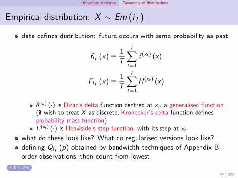
Empirical distribution: X ∼ Em (iT )
data defines distribution: future occurs with same probability as past
fiT (x) ≡ 1T
T∑t=1
δ(xt) (x)
FiT (x) ≡ 1T
T∑t=1
H(xt) (x)
δ(xt) (·) is Dirac’s delta function centred at xt , a generalised function(if wish to treat X as discrete, Kronecker’s delta function definesprobability mass function)H(xt) (·) is Heaviside’s step function, with its step at xt
what do these look like? What do regularised versions look like?defining QiT (p) obtained by bandwidth techniques of Appendix B:order observations, then count from lowest
X ∼ Em
36 / 229

Univariate statistics Taxonomy of distributions
Lecture 2 exercises
Meucci exercisespencil-and-paper: 1.2.5 (not Python), 1.2.6, 1.2.7Python: 1.2.3, 1.2.5 (Python)
projectinstall and configure Interactive Broker’s Python API; explore thedistribution of returns for your assets
37 / 229

Multivariate statistics Building blocks
Direct extensions of univariate statistics
if interested in portfolios (or even arbitrage), must be able to considerhow an asset’s movements depend on others’N-dimensional rv, X ≡ (X1, . . . ,XN)
′, so that x ∈ RN
probability density function
P X ∈ R ≡∫R
fX (x) dx, st fX (x) ≥ 0,∫RN
fX (x) dx = 1
cumulative or joint distribution function (df, DF, CDF, JDF . . . )
FX (x) ≡ P X ≤ x =
∫ x1
−∞· · ·∫ xN
−∞fX (u1, . . . , uN) duN · · · du1
characteristic function
ϕX (ω) ≡ E
eiω′X,ω ∈ RN
what about the quantile? (hint: FX : RN → R1)39 / 229
Multivariate statistics Building blocks
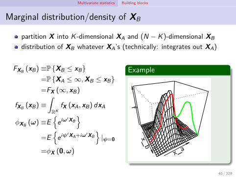
Marginal distribution/density of XB
partition X into K -dimensional XA and (N − K )-dimensional XB
distribution of XB whatever XA’s (technically: integrates out XA)
FXB (xB) ≡P XB ≤ xB=P XA ≤ ∞,XB ≤ xB=FX (∞, xB)
fXB (xB) ≡∫RK
fX (xA, xB) dxA
ϕXB (ω) ≡E
eiω′XB
=E
eiψ′XA+iω′XB|ψ=0
=ϕX (0,ω)
Example
x_b
x_a
f
40 / 229
Multivariate statistics Building blocks
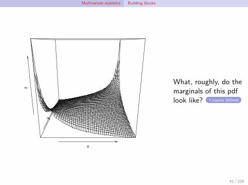
x
y
z
What, roughly, do themarginals of this pdflook like? copula defined
41 / 229
Multivariate statistics Building blocks
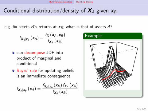
Conditional distribution/density of XA given xB
e.g. fix assets B’s returns at xB; what is that of assets A?
fXA|xB (xA) ≡fX (xA, xB)
fXB (xB)
can decompose JDF intoproduct of marginal andconditionalBayes’ rule for updating beliefsis an immediate consequence
fXA|xB (xA) =fXB |xA (xB) fXA (xA)
fXB (xB)
Example
x_b
x_a
f
42 / 229
Multivariate statistics Building blocks
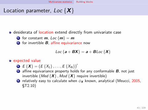
Location parameter, Loc X
desiderata of location extend directly from univariate case1 for constant m, Loc m = m2 for invertible B, affine equivariance now
Loc a + BX = a + BLoc X
expected value1 E X = (E X1 , . . . ,E XN)′2 affine equivariance property holds for any conformable B, not just
invertible (Med X ,Mod X require invertible)3 relatively easy to calculate when ϕX known, analytical (Meucci, 2005,
§T2.10)
43 / 229
Multivariate statistics Building blocks
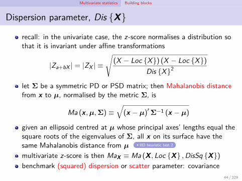
Dispersion parameter, Dis X
recall: in the univariate case, the z-score normalises a distribution sothat it is invariant under affine transformations
|Za+bX | = |ZX | ≡
√(X − Loc X) (X − Loc X)
Dis X2
let Σ be a symmetric PD or PSD matrix; then Mahalanobis distancefrom x to µ, normalised by the metric Σ, is
Ma (x,µ,Σ) ≡√
(x − µ)′Σ−1 (x − µ)
given an ellipsoid centred at µ whose principal axes’ lengths equal thesquare roots of the eigenvalues of Σ, all x on its surface have thesame Mahalanobis distance from µ IID heuristic test 2
multivariate z-score is then MaX ≡ Ma (X , Loc X ,DisSq X)benchmark (squared) dispersion or scatter parameter: covariance
44 / 229

Multivariate statistics Dependence
Correlation
normalised covariance
ρ (Xm,Xn) = Cor Xm,Xn ≡ Cov Xm,XnSd XmSd Xn
∈ [−1, 1]
where
Cov Xm,Xn ≡ E (Xm − E Xm) (Xn − E Xn)
when is this not defined?a measure of linear dependence, invariant under strictly increasinglinear transformations
ρ (αm + βmXm, αn + βnXn) = ρ (Xm,Xn)
fallacy (McNeil, Frey and Embrechts, 2015, p.241): given marginaldfs F1,F2 and any ρ ∈ [−1, 1], can always find a JDF F binding them
true for elliptical distributions; generally, attainable correlations are astrict subset of [−1, 1] (McNeil, Frey and Embrechts, 2015, Ex. 7.29)
conventional wisdom: during market stress, all correlations ⇒ 146 / 229
Multivariate statistics Dependence
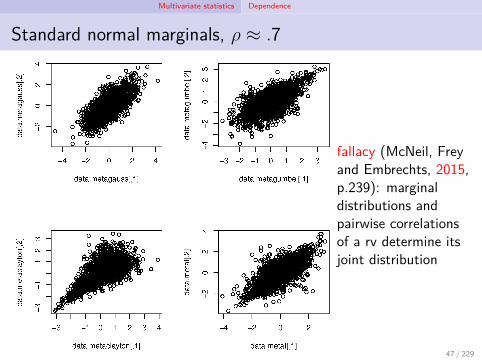
Standard normal marginals, ρ ≈ .7
fallacy (McNeil, Freyand Embrechts, 2015,p.239): marginaldistributions andpairwise correlationsof a rv determine itsjoint distribution
47 / 229
Multivariate statistics Dependence
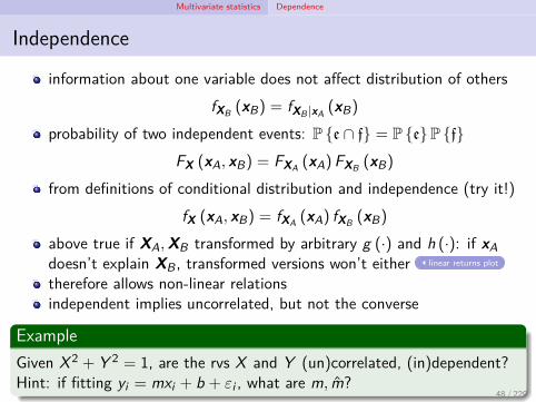
Independence
information about one variable does not affect distribution of othersfXB (xB) = fXB |xA (xB)
probability of two independent events: P e ∩ f = P eP fFX (xA, xB) = FXA (xA)FXB (xB)
from definitions of conditional distribution and independence (try it!)fX (xA, xB) = fXA (xA) fXB (xB)
above true if XA,XB transformed by arbitrary g (·) and h (·): if xAdoesn’t explain XB, transformed versions won’t either linear returns plot
therefore allows non-linear relationsindependent implies uncorrelated, but not the converse
ExampleGiven X 2 + Y 2 = 1, are the rvs X and Y (un)correlated, (in)dependent?Hint: if fitting yi = mxi + b + εi , what are m, m?
48 / 229

Multivariate statistics Taxonomy of distributions
Uniform distribution
idea is as in univariate case, but domain may be anythingoften elliptical domain, Eµ,Σ where µ is centroid, Σ is positive matrix
Example
fX1,X2 (x1, x2) =1πIx2
1+x22≤1 (x1, x2)
where IS is the indicator function on the set S
marginal density: fX1 (x1) =∫√1−x2
1
−√
1−x21
1πdx2 = 2
π
√1 − x2
1
conditional density: fX1|x2 (x1) =fX1,X2 (x1,x2)
fX2 (x2)= 1
2√
1−x22
are X1 and X2 (un)correlated, (in)dependent?
50 / 229
Multivariate statistics Taxonomy of distributions
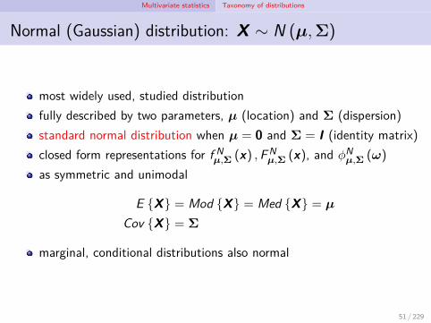
Normal (Gaussian) distribution: X ∼ N (µ,Σ)
most widely used, studied distributionfully described by two parameters, µ (location) and Σ (dispersion)standard normal distribution when µ = 0 and Σ = I (identity matrix)closed form representations for f N
µ,Σ (x) ,F Nµ,Σ (x), and ϕN
µ,Σ (ω)
as symmetric and unimodal
E X = Mod X = Med X = µ
Cov X = Σ
marginal, conditional distributions also normal
51 / 229
Multivariate statistics Taxonomy of distributions
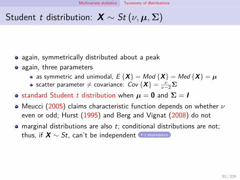
Student t distribution: X ∼ St (ν,µ,Σ)
again, symmetrically distributed about a peakagain, three parameters
as symmetric and unimodal, E X = Mod X = Med X = µscatter parameter = covariance: Cov X = ν
ν−2Σ
standard Student t distribution when µ = 0 and Σ = IMeucci (2005) claims characteristic function depends on whether νeven or odd; Hurst (1995) and Berg and Vignat (2008) do notmarginal distributions are also t; conditional distributions are not;thus, if X ∼ St, can’t be independent t dependence
52 / 229
Multivariate statistics Taxonomy of distributions
Cauchy distribution: X ∼ Ca (µ,Σ)
as in the univariate case, the fat-tailed limit of the Studentt-distribution: Ca (µ,Σ) = St (1,µ,Σ)
standard Cauchy distribution when µ = 0 and Σ = I (identity matrix)same problem with moments as univariate case
53 / 229

Multivariate statistics Taxonomy of distributions
Log-distributions
exponentials of other distributions, applied component-wisethus, useful for modelling positive valuesif Y has pdf fY then X ≡ eY is log-Y distributed
Example (Log-normal)Let Y ∼ N (µ,Σ). Then, if X ≡ eY , so that Xi ≡ eYi for all i = 1, . . . ,N,X ∼ LogN (µ,Σ).
54 / 229
Multivariate statistics Taxonomy of distributions
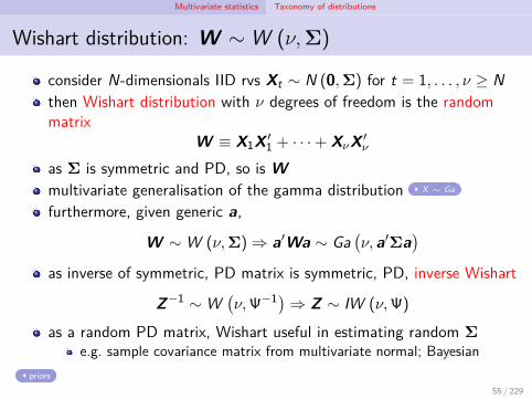
Wishart distribution: W ∼ W (ν,Σ)
consider N-dimensionals IID rvs Xt ∼ N (0,Σ) for t = 1, . . . , ν ≥ Nthen Wishart distribution with ν degrees of freedom is the randommatrix
W ≡ X1X ′1 + · · ·+ XνX ′
ν
as Σ is symmetric and PD, so is Wmultivariate generalisation of the gamma distribution X ∼ Ga
furthermore, given generic a,
W ∼ W (ν,Σ) ⇒ a′Wa ∼ Ga(ν, a′Σa
)as inverse of symmetric, PD matrix is symmetric, PD, inverse Wishart
Z−1 ∼ W(ν,Ψ−1)⇒ Z ∼ IW (ν,Ψ)
as a random PD matrix, Wishart useful in estimating random Σe.g. sample covariance matrix from multivariate normal; Bayesian
priors
55 / 229

Multivariate statistics Taxonomy of distributions
Empirical distribution: X ∼ Em (iT )
direct extension of univariate case X ∼ Em
fiT (x) ≡ 1T
T∑t=1
δ(xt) (x)
FiT (x) ≡ 1T
T∑t=1
H(xt) (x)
ϕiT (ω) ≡ 1T
T∑t=1
eiω′xt
moments include1 sample mean: EiT ≡ 1
T∑T
t=1 xt
2 sample covariance: ˆCov iT ≡ 1T∑T
t=1
(xt − EiT
)(xt − EiT
)′56 / 229

Multivariate statistics Special classes of distributions
Elliptical distributions: X ∼ El (µ,Σ, gN)
highly symmetrical, analytically tractable, flexibleX is elliptically distributed with location parameter µ and scattermatrix Σ if its iso-probability contours form ellipsoids centred at µwhose principal axes’ lengths are proportional to the square roots ofΣ’s eigenvalueselliptical pdf must be
fµ,Σ (x) = |Σ|−12 gN
(Ma2 (x,µ,Σ)
)where gN (·) ≥ 0 is a generator function rotated to form thedistribution.examples include: uniform (sometimes), normal, Student t, Cauchyaffine transformations: for any K -vector a, K × N matrix B, and theright generator gK ,
X ∼ El (µ,Σ, gN) ⇒ a + BX ∼ El(a + Bµ,BΣB′, gK
)correlation captures all dependence structure (copula adds nothing)
58 / 229

Multivariate statistics Special classes of distributions
Stable distributions
let X ,Y and Z be IID rvs; their distribution is stable if a linearcombination of them has the same distribution, up to location, scaleparameters: for any constants α, β > 0 there exist constants γ andδ > 0 such that
αX + βY d=γ + δZ
examples: normal, Cauchy (but not lognormal, or generic Student t)closed under linear combinations, thus allows easy projection toinvestment horizonsstability implies additivity (the sum of two IID rvs belongs to thesame family of distributions), but not the reverse
Example1 stable ⇒ additive: X ,Y ,Z ∼ NID
(1, σ2)⇒ X + Y d
= 2 −√
2 +√
2Z2 additive ⇒ stable:
X ,Y ,Z ∼ WID (ν,Σ) ⇒ X + Y ∼ W (2ν,Σ)d=γ + δZ
59 / 229

Multivariate statistics Special classes of distributions
Infinitely divisible distributions
the distribution of rv X is infinitely divisible if it can be expressed as. . . the sum of an arbitrary number of IID rvs: for any integer T
X d=Y1 + · · ·+ YT
for some IID rvs Y1, . . . ,YT
examples include: all elliptical, gamma, LogN (but not Wishart forN > 1)shall see: assists in projection to arbitrary investment horizons (e.g.any T )
60 / 229

Multivariate statistics Special classes of distributions
Lecture 3 exercises
Meucci exercisespencil-and-paper: 1.3.1, 1.3.4, 2.1.3Python: 1.2.8, 1.3.2, 1.3.3, 2.1.1, 2.1.2
projectpick a trading algorithm you plan to use and develop.can you fit standard distributions to your assets’ compound returns(univariate and multivariate)?
61 / 229

Multivariate statistics Copulas
Introductionthe copula is a standardized version of the purely joint features of amultivariate distribution, which is obtained by filtering out all thepurely one-dimensional features, namely the marginal distributionof each entry Xn. (Meucci, 2005, p.40)
McNeil, Frey and Embrechts (2015, Ch 7) goes into more detail than(Meucci, 2005, Ch 2) on copulas
more material about the book is available at www.qrmtutorial.orgsee Embrechts (2009) for thoughts on the “copula craze”, from oneof its pioneers, and a “must-read” for contextthe classic text is Nelsen (2006); it contains worked examples and setquestions, and has the space to properly develop the basic conceptsa 2009 wired.com article blamed the Gaussian copula formula for“killing” Wall Street
63 / 229

Multivariate statistics Copulas
Copulas defined
DefinitionAn N-dimensional copula, U, is defined on [0, 1]N ; its JDF, FU , hasstandard uniform marginal distributions.
copula example
Embrechts (2009, p.640) notes that other standardisations than thecopula’s to the unit hypercube may sometimes be more useful
64 / 229
Multivariate statistics Copulas
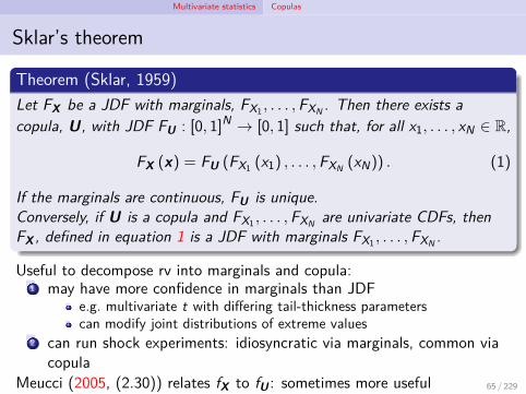
Sklar’s theorem
Theorem (Sklar, 1959)Let FX be a JDF with marginals, FX1 , . . . ,FXN . Then there exists acopula, U, with JDF FU : [0, 1]N → [0, 1] such that, for all x1, . . . , xN ∈ R,
FX (x) = FU (FX1 (x1) , . . . ,FXN (xN)) . (1)
If the marginals are continuous, FU is unique.Conversely, if U is a copula and FX1 , . . . ,FXN are univariate CDFs, thenFX , defined in equation 1 is a JDF with marginals FX1 , . . . ,FXN .
Useful to decompose rv into marginals and copula:1 may have more confidence in marginals than JDF
e.g. multivariate t with differing tail-thickness parameterscan modify joint distributions of extreme values
2 can run shock experiments: idiosyncratic via marginals, common viacopula
Meucci (2005, (2.30)) relates fX to fU : sometimes more useful 65 / 229
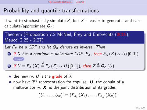
Multivariate statistics Copulas
Probability and quantile transformationsIf want to stochastically simulate Z , but X is easier to generate, and cancalculate/approximate QZ :
Theorem (Proposition 7.2 McNeil, Frey and Embrechts (2015);Meucci 2.25 - 2.27)Let FX be a CDF and let QX denote its inverse. Then
1 if X has a continuous univariate CDF, FX , then FX (X ) ∼ U ([0, 1])proof
2 if U ≡ FX (X )d=FZ (Z ) ∼ U ([0, 1]), then Z d
=QZ (U)
the new rv, U is the grade of Xnow have 3rd representation for copulas: U, the copula of amultivariate rv, X , is the joint distribution of its grades
(U1, . . . ,UN)′ ≡ (FX1 (X1) , . . . ,FXN (XN))
′
66 / 229

Multivariate statistics Copulas
Independence copula
independence of rvs ⇔ JDF is the product of their univariate CDFsapplying Sklar’s theorem to independent rvs, X1, . . . ,XN
FX (x) =N∏
n=1FXn (xn) = FU (FX1 (x1) , . . . ,FXN (xN))
thus, substituting FXn (xn) = un, provides the independence copula
Π (u) ≡ FU (u1, . . . , uN) =N∏
n=1un
which is uniformly distributed on the unit hyper-cube, with ahorizontal pdf, π (u) = 1Schweizer-Wolf measures of dependence (indexed by p in Lp-norm):distance between a copula and the independence copula
67 / 229

Multivariate statistics Copulas
Strictly increasing transformations of the marginals
recall: correlation only invariant under linear transformations
Theorem (Proposition 7.7 McNeil, Frey and Embrechts (2015))Let (X1, . . . ,XN) be a rv with continuous marginals and copula U, and letg1, . . . , gN be strictly increasing functions. Then (g1 (X1) , . . . , gN (XN))also has copula U.
a special case of this is the co-monotonicity copulalet the rvs X1, . . . ,XN have continuous dfs that are perfectly positivelydependent, so that Xn = gn (X1) almost surely for all n ∈ 2, . . . ,Nfor strictly increasing gn (·)co-monotonicity copula is then
M (u) ≡ min u1, . . . , uN
where the JDF of the rv (U, . . . ,U) is s.t. U ∼ U ([0, 1]) (McNeil, Freyand Embrechts, 2015, p.226)
68 / 229

Multivariate statistics Copulas
Fréchet-Hoeffding bounds
co-monotonicity copula, M, isFréchet-Hoeffding upper boundFréchet-Hoeffding lower bound,W , isn’t copula for N > 2:
W (u) ≡ max
1 − N +
N∑n=1
un, 0
any copula’s CDF fits betweenthese
W (u) ≤ FU (u) ≤ M (u)
which copula is 2nd figure?R code: Härdle and Okhrin(2010)
69 / 229

Multivariate statistics Copulas
A call option
ExampleConsider two stock prices, the rvs X = (X1,X2), and a European calloption on the first with strike price K . The payoff on this option istherefore also a rv, C1 ≡ max X1 − K , 0.Thus, C1 and X1 are co-monotonic; their copula is M, the co-monotonicitycopula. Further, (X1,X2) and (C1,X2) are also co-monotonic; the copulaof (X1,X2) is the same as that of (C1,X2).What technical detail is the above missing? How is this overcome?
co-monotonic additivity
70 / 229

Modelling the market
Conceptual overview
Meucci (2005) identifies the following steps for building the link betweenhistorical performance and future distributions
1 detecting the invariantswhat market variables can be modelled as IID rvs?Meucci (2017): risk drivers are time-homogenous variables drivingP&L; invariants are their IID shocks
2 determining the distribution of the invariantshow frequently do these change (q.v. Bauer and Braun (2010))?
3 projecting the invariants into the future4 mapping the invariants into the market prices
As the dimension of ‘most’ randomness may be much less than that of theportfolio space, dimension reduction techniques will enhance tractability
71 / 229
Modelling the market Stylised facts
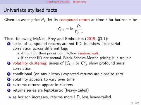
Univariate stylised factsGiven an asset price Pt , let its compound return at time t for horizon τ be
Ct,τ ≡ lnPt
Pt−τ
Then, following McNeil, Frey and Embrechts (2015, §3.1):1 series of compound returns are not IID, but show little serial
correlation across different lagsif not IID, then prices don’t follow random walkif neither IID nor normal, Black-Scholes-Merton pricing is in trouble
2 volatility clustering: series of |Ct,τ | or C2t,τ show profound serial
correlation3 conditional (on any history) expected returns are close to zero4 volatility appears to vary over time5 extreme returns appear in clusters6 returns series are leptokurtic (heavy-tailed)
as horizon increases, returns more IID, less heavy-tailed73 / 229
Modelling the market Stylised facts
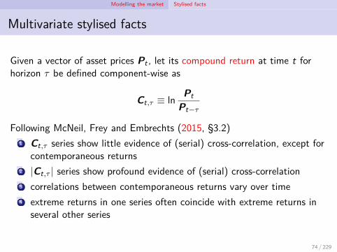
Multivariate stylised facts
Given a vector of asset prices Pt , let its compound return at time t forhorizon τ be defined component-wise as
Ct,τ ≡ lnPt
Pt−τ
Following McNeil, Frey and Embrechts (2015, §3.2)1 Ct,τ series show little evidence of (serial) cross-correlation, except for
contemporaneous returns2 |Ct,τ | series show profound evidence of (serial) cross-correlation3 correlations between contemporaneous returns vary over time4 extreme returns in one series often coincide with extreme returns in
several other series
74 / 229
Modelling the market The quest for invariance
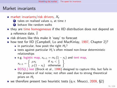
Market invariants
market invariants/risk drivers, Xt1 takes on realised values xt at time t2 behave like random walks
they are time homogeneous if the IID distribution does not depend ona reference date, trisk drivers like this make it ‘easy’ to forecasthow test for IID (Campbell, Lo and MacKinlay, 1997, Chapter 2)?
in particular, how posit the right H1?tests against particular H1’s often missed non-linear deterministicrelationshipse.g. logistic map, xt+1 = rxt (1 − xt) and tent map,
xt+1 =
µxt if xt <
12
µ (1 − xt) otherwise
BDS(L) test (Brock et al., 1996) designed to capture this, but fails inthe presence of real noise; not often used due to strong theoreticalpriors on H1
we therefore present two heuristic tests (q.v. Meucci, 2009, §2)76 / 229
Modelling the market The quest for invariance
Heuristic test 1: compare split sample histograms
by the Glivenko-Cantelli theorem, empirical pdf → true pdf as thenumber of IID observations growssplit the time series in half and compare the two histogramswhat should the two histograms look like if IID?
77 / 229
Modelling the market The quest for invariance
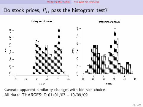
Do stock prices, Pt , pass the histogram test?
Caveat: apparent similarity changes with bin size choiceAll data: THARGES:ID 01/01/07 – 10/09/09
78 / 229

Modelling the market The quest for invariance
Do linear stock returns, Lt,τ , pass the histogram test?
Linear returns are Lt,τ ≡ PtPt−τ
− 1
79 / 229
Modelling the market The quest for invariance
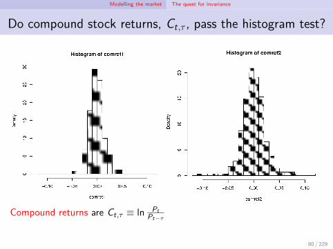
Do compound stock returns, Ct,τ , pass the histogram test?
Compound returns are Ct,τ ≡ ln PtPt−τ
80 / 229
Modelling the market The quest for invariance
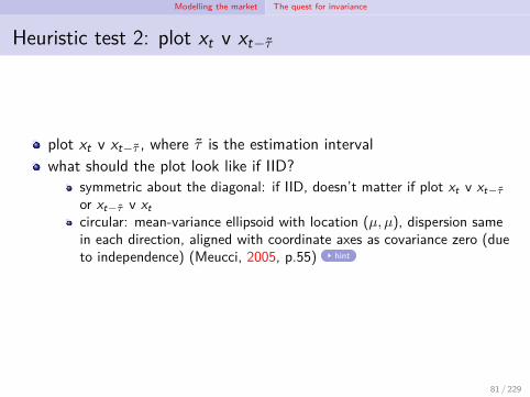
Heuristic test 2: plot xt v xt−τ
plot xt v xt−τ , where τ is the estimation intervalwhat should the plot look like if IID?
symmetric about the diagonal: if IID, doesn’t matter if plot xt v xt−τor xt−τ v xtcircular: mean-variance ellipsoid with location (µ, µ), dispersion samein each direction, aligned with coordinate axes as covariance zero (dueto independence) (Meucci, 2005, p.55) hint
81 / 229
Modelling the market The quest for invariance
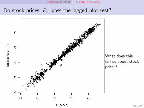
Do stock prices, Pt , pass the lagged plot test?
What does thistell us about stockprices?
82 / 229
Modelling the market The quest for invariance
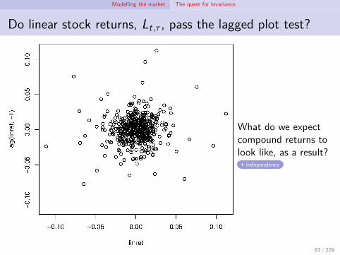
Do linear stock returns, Lt,τ , pass the lagged plot test?
What do we expectcompound returns tolook like, as a result?
independence
83 / 229
Modelling the market The quest for invariance
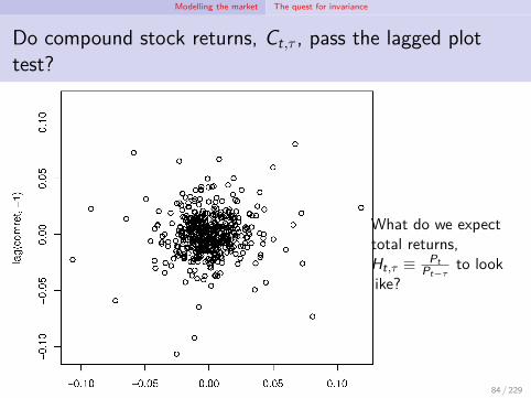
Do compound stock returns, Ct,τ , pass the lagged plottest?
What do we expecttotal returns,Ht,τ ≡ Pt
Pt−τto look
like?
84 / 229
Modelling the market The quest for invariance
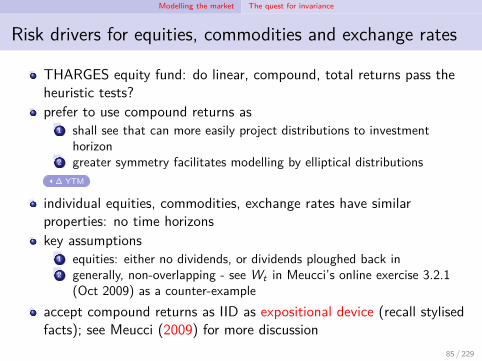
Risk drivers for equities, commodities and exchange rates
THARGES equity fund: do linear, compound, total returns pass theheuristic tests?prefer to use compound returns as
1 shall see that can more easily project distributions to investmenthorizon
2 greater symmetry facilitates modelling by elliptical distributions∆ YTM
individual equities, commodities, exchange rates have similarproperties: no time horizonskey assumptions
1 equities: either no dividends, or dividends ploughed back in2 generally, non-overlapping - see Wt in Meucci’s online exercise 3.2.1
(Oct 2009) as a counter-exampleaccept compound returns as IID as expositional device (recall stylisedfacts); see Meucci (2009) for more discussion
85 / 229

Modelling the market The quest for invariance
Lecture 4 exercises
Nelsen (2006, Exercise 2.12) Let X and Y be rvs with JDF
H (x , y) =(1 + e−x + e−y)−1
for all x , y ∈ R, the extended reals.1 show that X and Y have standard (univariate) logistic distributions
F (x) =(1 + e−x)−1 and G (y) =
(1 + e−y)−1
.
2 show that the copula of X and Y is C (u, v) = uvu+v−uv .
Meucci exercisespencil-and-paper: 3.2.1Python: 2.2.1, 2.2.3, 2.2.4, 2.2.6, 3.1.3
projectuse the IB API to execute trades algorithmically.do your assets’ compound returns appear invariant, or do they displayGARCH properties?
86 / 229

Modelling the market The quest for invariance
Fixed income: zero-coupon bonds
make no termly paymentsas simplest form of bond, form basis for analysis of bondsfixed income as certain [?] payout at face or redemption value
(see Brigo, Morini and Pallavicini (2013) for richer risk modelling)
bond price then Z (E)t , where t ≤ E is date, and E is maturity date
normalise Z (E)E = 1
are bond prices invariants?1 stock prices weren’t2 time homogeneity violated
are returns (total, simple, compound) invariants?
87 / 229

Modelling the market The quest for invariance
Fixed income: a time homogeneous frameworkconstruct a synthetic series of bond prices with the same time tomaturity, v :
1 Z (E)t (e.g. Nov 2018 price of a bond that matures in Feb 2023)
2 Z (E−τ)t−τ (e.g. Nov 2017 price of a bond that matures in Feb 2022)
3 Z (E−2τ)t−2τ (e.g. Nov 2016 price of a bond that matures in Feb 2021)
4...
target duration funds: an established fixed income strategy(Langetieg, Leibowitz and Kogelman, 1990)can now define pseudo-returns, or rolling (total) returns to maturity
R(v)t,τ ≡ Z (t+v)
t
Z (t−τ+v)t−τ
where τ is the estimation interval (e.g. a year)candidates for passing the two heuristic tests (Meucci, 2005, Figure3.5)
88 / 229
Modelling the market The quest for invariance
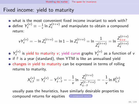
Fixed income: yield to maturity
what is the most convenient fixed income invariant to work with?define Y (v)
t ≡ − 1v lnZ (t+v)
t and manipulate to obtain a compoundreturn:
vY (v)t = − lnZ (t+v)
t = ln 1 − lnZ (t+v)t = ln
1Z (t+v)
t= ln
Z (t+v)t+v
Z (t+v)t
Y (v)t is yield to maturity v ; yield curve graphs Y (v)
t as a function of vif τ is a year (standard), then YTM is like an annualised yieldchanges in yield to maturity can be expressed in terms of rollingreturns to maturity,
X (v)t,τ ≡ Y (v)
t − Y (v)t−τ = −1
v lnZ (t+v)
t
Z (t−τ+v)t−τ
= −1v lnR(v)
t,τ
usually pass the heuristics, have similarly desirable properties tocompound returns for equities compound returns
89 / 229
Modelling the market The quest for invariance
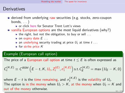
Derivativesderived from underlying raw securities (e.g. stocks, zero-couponbonds, . . . )
or click here for Senator Trent Lott’s viewsvanilla European options are the most liquid derivatives (why?)
the right, but not the obligation, to buy or sell . . .on expiry date E . . .an underlying security trading at price Ut at time t . . .for strike price K
Example (European call option)The price of a European call option at time t ≤ E is often expressed as
C (K ,E)t ≡ CBSM
(E − t,K ,Ut ,Z (E)
t , σ(K ,E)t
)s.t.C (K ,E)
E = max UE − K , 0
where E − t is the time remaining, and σ(K ,E)t is the volatility of Ut .
The option is in the money when Ut > K , at the money when Ut = K andout of the money otherwise.
90 / 229

Modelling the market The quest for invariance
Derivatives: volatilitypricing options requires a measure of volatility
1 historical or realised volatility: determined from historical values of Ut(esp. ARCH models); backward looking but model-free
2 implied volatility: as the call option’s price increases in σt , the BSMpricing formula has an inverse, allowing volatility to be implied fromoption prices; forward looking, but model-dependent; e.g. VXO
3 model-free volatility expectations: risk-neutral expectation of OTMoption prices; forward looking, less model-dependent (but assumesstochastic process doesn’t jump); e.g. VIX
Taylor, Yadav and Zhang (2010) compare the three volatilitymeasuresat-the-money-forward (ATMF) implied percentage volatility of theunderlying: “implied percentage volatility of an option whose strike isequal to the forward price of the underlying at expiry” (Meucci, 2005)
Kt =Ut
Z (E)t
= ert(E−t)Ut , where latter rearranges the no-arbitrage
forward price formula (Stefanica, 2011, §1.10), Z (E)t ert(E−t) = 1
why ATMF? 91 / 229
Modelling the market The quest for invariance
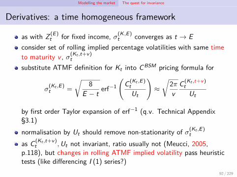
Derivatives: a time homogeneous framework
as with Z (E)t for fixed income, σ(K ,E)
t converges as t → Econsider set of rolling implied percentage volatilities with same timeto maturity v , σ(Kt ,t+v)
tsubstitute ATMF definition for Kt into CBSM pricing formula for
σ(Kt ,E)t =
√8
E − t erf−1
(C (Kt ,E)
tUt
)≈√
2πv
C (Kt ,t+v)t
Ut
by first order Taylor expansion of erf−1 (q.v. Technical Appendix§3.1)normalisation by Ut should remove non-stationarity of σ(Kt ,E)
t
as C (Kt ,t+v)t ,Ut not invariant, ratio usually not (Meucci, 2005,
p.118), but changes in rolling ATMF implied volatility pass heuristictests (like differencing I (1) series?)
92 / 229
Modelling the market Projecting invariants to the investment horizon
Projecting invariants to the investment horizon
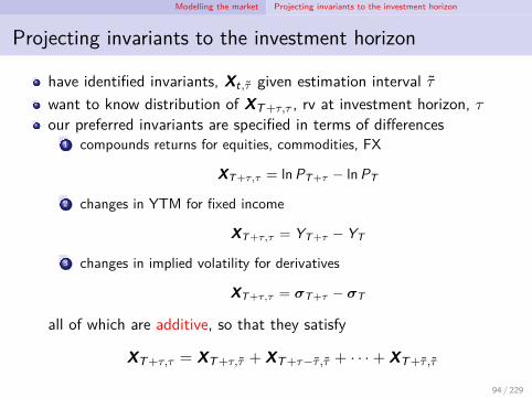
have identified invariants, Xt,τ given estimation interval τwant to know distribution of XT+τ,τ , rv at investment horizon, τour preferred invariants are specified in terms of differences
1 compounds returns for equities, commodities, FX
XT+τ,τ = lnPT+τ − lnPT
2 changes in YTM for fixed income
XT+τ,τ = YT+τ − YT
3 changes in implied volatility for derivatives
XT+τ,τ = σT+τ − σT
all of which are additive, so that they satisfy
XT+τ,τ = XT+τ,τ + XT+τ−τ ,τ + · · ·+ XT+τ ,τ
94 / 229

Modelling the market Projecting invariants to the investment horizon
Distributions at the investment horizonfor expositional simplicity, assume that τ = k τ , where k ∈ Z++
no problem if not as long as distribution is infinitely divisible (why?)as all of the invariants in
XT+τ,τ = XT+τ,τ + XT+τ−τ ,τ + · · ·+ XT+τ ,τ
are IID, the projection formula is
ϕXT+τ,τ=(ϕXt,τ
) ττ
proof
can translate back and forth between cf and pdf with Fourier andinverse Fourier transforms
ϕX = F [fX ] and fX = F−1 [ϕX ]
by contrast, linear return projections yieldLT+τ,τ = diag (1 + LT+τ,τ )× · · · × diag (1 + LT+τ ,τ )− 1
where the diagonal entries in the N × N diag matrix are those in itsvector-valued argument; its off-diagonal entries are zero 95 / 229

Modelling the market Projecting invariants to the investment horizon
Joint normal distributions
ExampleLet the weekly compound returns on a stock and the weekly yield changesfor three-year bonds be normally distributed. Thus, the invariants are
Xt,τ =
(Ct,τ
X (v)t,τ
)≡
(lnPt − lnPt−τ
Y (v)t − Y (v)
t−τ
).
Bind these marginals so that their joint distribution is also normal,Xt,τ ∼ N (µ,Σ). By joint normality, the cf is ϕXt,τ (ω) = eiω′µ− 1
2ω′Σω.
From the previous slide, XT+τ,τ has cf ϕXT+τ,τ(ω) = eiω′ τ
τµ− 1
2ω′ ττΣω.
Thus,XT+τ,τ ∼ N
(ττµ,τ
τΣ).
96 / 229
Modelling the market Projecting invariants to the investment horizon
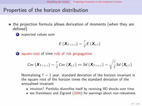
Properties of the horizon distribution
the projection formula allows derivation of moments (when they aredefined)
1 expected values sum
E XT+τ,τ =τ
τE Xt,τ
2 square-root of time rule of risk propagation
Cov XT+τ,τ =τ
τCov Xt,τ ⇔ Sd XT+τ,τ =
√τ
τSd Xt,τ
Normalising τ = 1 year: standard deviation of the horizon invariant isthe square root of the horizon times the standard deviation of theannualised invariant
intuition? Portfolio diversifies itself by receiving IID shocks over timesee Danielsson and Zigrand (2006) for warnings about non-robustness
97 / 229
Modelling the market Mapping invariants into market prices
Raw securities: horizon prices
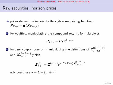
prices depend on invariants through some pricing function,PT+τ = g (XT+τ,τ )
1 for equities, manipulating the compound returns formula yields
PT+τ = PT eXT+τ,τ
2 for zero coupon bounds, manipulating the definitions of R(E−T−τ)T+τ,τ
and X(E−T−τ)T+τ,τ yields
Z (E)T+τ = Z (E−τ)
T e−(E−T−τ)X(E−T−τ)T+τ,τ
n.b. could use v ≡ E − (T + τ)
99 / 229

Modelling the market Mapping invariants into market prices
Raw securities: horizon price distribution
for both equities and fixed income, PT+τ = eYT+τ,τ , where
YT+τ,τ ≡ γ + diag (ε)XT+τ,τ
an affine transformationthus, they have a log−Y distributionthis can be represented as
ϕYT+τ,τ(ω) = eiω′γϕXT+τ,τ
(diag (ε)ω)
usually impossible to compute closed form for full distributionmay suffice just to compute first few momentse.g. can compute E Pn and Cov Pm,Pn from cf
100 / 229
Modelling the market Mapping invariants into market prices
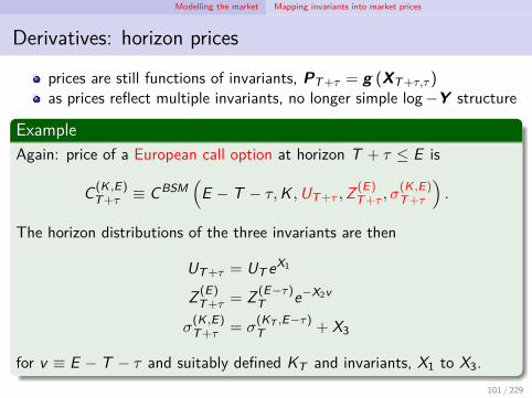
Derivatives: horizon prices
prices are still functions of invariants, PT+τ = g (XT+τ,τ )as prices reflect multiple invariants, no longer simple log−Y structure
ExampleAgain: price of a European call option at horizon T + τ ≤ E is
C (K ,E)T+τ ≡ CBSM
(E − T − τ,K ,UT+τ ,Z (E)
T+τ , σ(K ,E)T+τ
).
The horizon distributions of the three invariants are then
UT+τ = UT eX1
Z (E)T+τ = Z (E−τ)
T e−X2v
σ(K ,E)T+τ = σ
(KT ,E−τ)T + X3
for v ≡ E − T − τ and suitably defined KT and invariants, X1 to X3.101 / 229
Modelling the market Mapping invariants into market prices
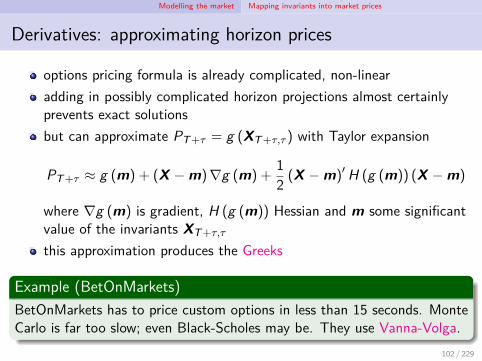
Derivatives: approximating horizon prices
options pricing formula is already complicated, non-linearadding in possibly complicated horizon projections almost certainlyprevents exact solutionsbut can approximate PT+τ = g (XT+τ,τ ) with Taylor expansion
PT+τ ≈ g (m) + (X − m)∇g (m) +12 (X − m)′ H (g (m)) (X − m)
where ∇g (m) is gradient, H (g (m)) Hessian and m some significantvalue of the invariants XT+τ,τ
this approximation produces the Greeks
Example (BetOnMarkets)BetOnMarkets has to price custom options in less than 15 seconds. MonteCarlo is far too slow; even Black-Scholes may be. They use Vanna-Volga.
102 / 229

Modelling the market Mapping invariants into market prices
Lecture 5 exercises
Meucci exercisespencil-and-paper: 5.3Python: 3.2.2, 3.2.3, 5.1 (modify code to display one-period andhorizon distributions; contrast to Meucci (2005) equations 3.95, 3.96),5.5.1, 5.5.2, 5.6
projectproduce horizon price distributions for your assets (ideally using fullymultivariate techniques) by means of one of the techniques mentionedin Daníelsson (2015) and a technique in scikit-learn.
103 / 229

Modelling the market Dimension reduction
Why dimension reduction?
1 actual dimension of the market is less than the number of securities
ExampleConsider a stock whose price is Ut and a European call option on it withstrike K and expiry date T + τ . Their horizon prices are
PT+τ =
(UT+τ
max UT+τ − K , 0
).
These are perfectly positively dependent.
2 randomness in the market can be well approximated with fewer thanN dimensions (that of the market invariants, X)
this is the possibility considered in what followscan considerably reduce computational complexity
105 / 229
Modelling the market Dimension reduction
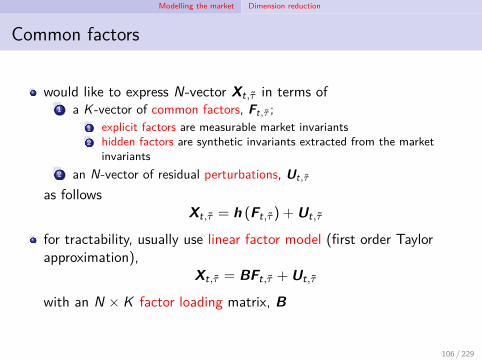
Common factors
would like to express N-vector Xt,τ in terms of1 a K -vector of common factors, Ft,τ ;
1 explicit factors are measurable market invariants2 hidden factors are synthetic invariants extracted from the market
invariants2 an N-vector of residual perturbations, Ut,τ
as followsXt,τ = h (Ft,τ ) + Ut,τ
for tractability, usually use linear factor model (first order Taylorapproximation),
Xt,τ = BFt,τ + Ut,τ
with an N × K factor loading matrix, B
106 / 229

Modelling the market Dimension reduction
Common factors: desiderata
1 substantial dimension reduction, K ≪ N2 independence of Ft,τ and Ut,τ (why?)
hard to attain, so often relax to Cor Ft,τ ,Ut,τ = 0K×N3 goodness of fit
want recovered invariants to be close, X ≡ h (F ) ≈ Xuse generalised R2
R2
X , X≡ 1 −
E(
X − X)′ (
X − X)
tr Cov X
where the trace of Y , tr Y, is the sum of its diagonal entries1 what is in the numerator?2 what is in the denominator?3 how does this differ from the usual coefficient of determination, R2?
107 / 229

Modelling the market Dimension reduction
Explicit factors
suppose that theory provides a list of explicit market variables asfactors, Fhow does one determine the loadings matrix, B?with linear factor model, X = BF + U, pick B to maximisegeneralised R2
Br ≡ argmaxB
R2 X ,BF
where the subscript indicates that these are determined by regressionthis is solved by
Br = E
XF ′E
FF ′−1
how does this differ from OLS?even weak version of second desideratum, Cor F ,U = 0K×N notgenerally satisfied; but:
1 E F = 0 ⇒ Cor F ,U = 0K×N2 adding constant factor to F ⇒ E Ur = 0,Cor F ,Ur = 0K×N
cf. including constant term in OLS regression108 / 229
Modelling the market Dimension reduction
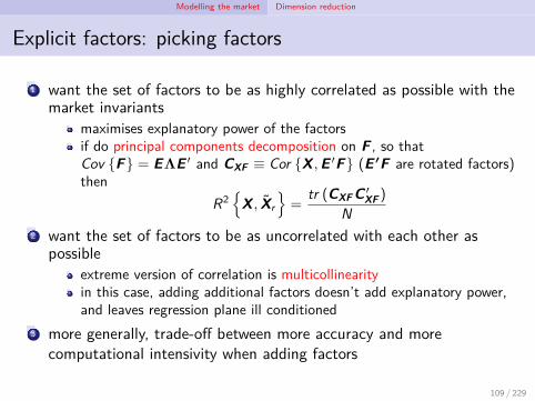
Explicit factors: picking factors
1 want the set of factors to be as highly correlated as possible with themarket invariants
maximises explanatory power of the factorsif do principal components decomposition on F , so thatCov F = EΛE ′ and CXF ≡ Cor X ,E ′F (E ′F are rotated factors)then
R2
X , Xr
=
tr (CXF C ′XF )
N2 want the set of factors to be as uncorrelated with each other as
possibleextreme version of correlation is multicollinearityin this case, adding additional factors doesn’t add explanatory power,and leaves regression plane ill conditioned
3 more generally, trade-off between more accuracy and morecomputational intensivity when adding factors
109 / 229

Modelling the market Dimension reduction
Example (Capital assets pricing model (CAPM))
The linear returns (invariants) of N stocks are L(n)t,τ ≡ P(n)
tP(n)
t−τ
− 1. If the priceof the market index is Mt , the linear return on the market index,F M
t,τ ≡ MtMt−τ
− 1, is a linear factor. The general regression result (3.127)then reduces, in this special case, to:
L(n)t,τ = E
L(n)
t,τ
+ β
(n)τ
(F M
t,τ − E
F Mt,τ
).
Assuming mean-variance utility and efficient markets, linear returns lie onthe security market line
E
L(n)t,τ
= β
(n)τ E
F M
t,τ
+(
1 − β(n)τ
)R f
t,τ
where R ft,τ are risk-free returns (q.v. Dybvig and Ross, 1985). The CAPM
then followsL(n)
t,τ = R ft,τ + β
(n)τ
(F M
t,τ − R ft,τ
).
110 / 229
Modelling the market Dimension reduction
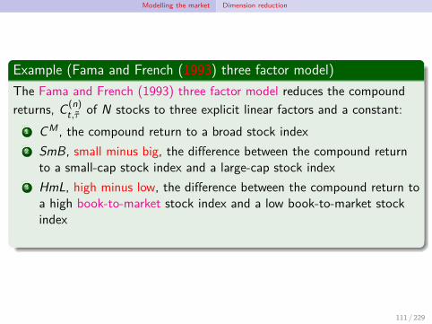
Example (Fama and French (1993) three factor model)The Fama and French (1993) three factor model reduces the compoundreturns, C (n)
t,τ of N stocks to three explicit linear factors and a constant:1 CM , the compound return to a broad stock index2 SmB, small minus big, the difference between the compound return
to a small-cap stock index and a large-cap stock index3 HmL, high minus low, the difference between the compound return to
a high book-to-market stock index and a low book-to-market stockindex
111 / 229
Modelling the market Dimension reduction
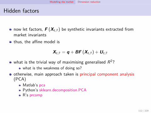
Hidden factors
now let factors, F (Xt,τ ) be synthetic invariants extracted frommarket invariantsthus, the affine model is
Xt,τ = q + BF (Xt,τ ) + Ut,τ
what is the trivial way of maximising generalised R2?what is the weakness of doing so?
otherwise, main approach taken is principal component analysis(PCA)
Matlab’s pcaPython’s sklearn.decomposition.PCAR’s prcomp
112 / 229
Modelling the market Dimension reduction
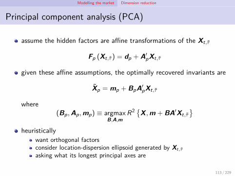
Principal component analysis (PCA)
assume the hidden factors are affine transformations of the Xt,τ
Fp (Xt,τ ) = dp + A′pXt,τ
given these affine assumptions, the optimally recovered invariants are
Xp = mp + BpA′pXt,τ
where(Bp,Ap,mp) ≡ argmax
B,A,mR2 X ,m + BA′Xt,τ
heuristically
want orthogonal factorsconsider location-dispersion ellipsoid generated by Xt,τasking what its longest principal axes are
113 / 229
Modelling the market Dimension reduction
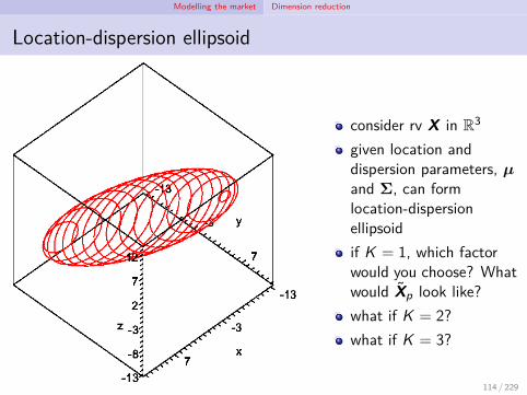
Location-dispersion ellipsoid
consider rv X in R3
given location anddispersion parameters, µand Σ, can formlocation-dispersionellipsoidif K = 1, which factorwould you choose? Whatwould Xp look like?what if K = 2?what if K = 3?
114 / 229
Modelling the market Dimension reduction
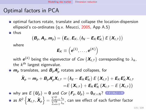
Optimal factors in PCA
optimal factors rotate, translate and collapse the location-dispersionellipsoid’s co-ordinates (q.v. Meucci, 2005, App A.5)thus
(Bp,Ap,mp) =(EK ,EK ,
(IN − EK E ′
K)
E Xt,τ)
whereEK ≡
(e(1), . . . , e(K)
)with e(k) being the eigenvector of Cov Xt,τ corresponding to λk ,the kth largest eigenvalue.mp translates, and BpA′
p rotates and collapses, for
Xp = mp + BpA′pXt,τ =
(IN − EK E ′
K)
E Xt,τ+ EK E ′K Xt,τ
=E Xt,τ+ EK E ′K (Xt,τ − E Xt,τ)
why are E Up = 0 and Cor Fp,Up = 0K×N? E
Up
= 0
as R2
Xt,τ , Xp=
∑Kk=1 λk∑Nn=1 λn
, can see effect of each further factor115 / 229
Modelling the market Dimension reduction
Explicit factors v PCA?
as PCA projects onto the most informative K dimensions, it yields ahigher R2 than any K -factor explicit factor modelhowever, the synthetic dimensions of PCA are harder to interpret, andtherefore perhaps to understand
but see Meucci (2005, Fig 3.19, p.158) for a decomposition of theswap market yield curve into level, slope and curvature factors
are PCA factors less stable out of sample?see pp.67- of Smith and Fuertes’ Panel Time Series notes for adiscussion of how to use and interpret PCA models
116 / 229
Estimating market invariants
The variance-bias tradeoff: what should an estimator do?
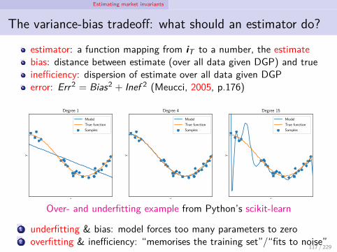
estimator: a function mapping from iT to a number, the estimatebias: distance between estimate (over all data given DGP) and trueinefficiency: dispersion of estimate over all data given DGPerror: Err2 = Bias2 + Inef 2 (Meucci, 2005, p.176)
x
y
Degree 1
ModelTrue functionSamples
x
y
Degree 4
ModelTrue functionSamples
x
y
Degree 15
ModelTrue functionSamples
Over- and underfitting example from Python’s scikit-learn
1 underfitting & bias: model forces too many parameters to zero2 overfitting & inefficiency: “memorises the training set”/“fits to noise”
117 / 229

Estimating market invariants
Example (Estimating the mean in small samples)Let X correspond to an independent throw of a fair die, so thatE X = µ = 7
2 . Suppose we do not know µ, but wish to estimate it.The sample mean, s ≡ 1
T∑T
t=1 xt is unbiased, E s − µ = 0, but may beinefficient as Var s ≡ E
(s − µ)2
may be high. When T = 1, for
example,
Var s =16
[254 +
94 +
14
]× 2 =
3512 < 3.
When T = 2,Var s = · · · = 105
72 <3512 .
Thus, when T = 2, s has an error of√
0 + 10572 =
√3524 . When T = 1, the
error is√
3.The fixed estimator s ≡ 2 has a bias of 3
2 , butVar s = E
(s − 2)2
= 0, for an error of 3
2 – better than s for T = 1,but worse when T ≥ 2.
118 / 229

Estimating market invariants
A rose by any other name1 classical econometric parlance
1 non-parametric estimators no identifying restrictions on the empiricaldistribution ⇒ good estimates require large samples
2 parametric estimators restrict distributions, so can estimate well onsmall samples (unless bad parametric restrictions have been made)
3 shrinkage estimators: for the smallest samples, perform Bayesianaverages of estimated values with a constant, reducing error byimproving efficiency at the cost of bias Bayes-Stein sample-based allocation
2 machine learning parlance (Kolanovic and Krishnamachari, 2017)1 supervised ML
1 regressions (continuous DV): parametric (e.g. ridge, lasso) &non-parametric (e.g. k-NN)
2 classifications (discrete DV): inc. logit, probit, SVM, decision tree,random forest, HMM
2 unsupervised ML: clustering (e.g. k-means, ward, birch) & factoranalyses (e.g. PCA)
3 deep/reinforcement learning: ‘neurons’ provide input to the next layerif linear scores exceeed threshold; most useful for images, text so far
119 / 229
Estimating market invariants
Weighted estimates
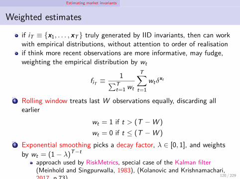
if iT ≡ x1, . . . , xT truly generated by IID invariants, then can workwith empirical distributions, without attention to order of realisationif think more recent observations are more informative, may fudge,weighting the empirical distribution by wt
fiT ≡ 1∑Tt=1 wt
T∑t=1
wtδxt
1 Rolling window treats last W observations equally, discarding allearlier
wt = 1 if t > (T − W )
wt = 0 if t ≤ (T − W )
2 Exponential smoothing picks a decay factor, λ ∈ [0, 1], and weightsby wt = (1 − λ)T−t
approach used by RiskMetrics, special case of the Kalman filter(Meinhold and Singpurwalla, 1983), (Kolanovic and Krishnamachari,2017, p.73)when T → ∞, converges to a GARCH model
120 / 229

Estimating market invariants
Lecture 6 exercises
Meucci exercisespencil-and-paper: 6.2.1, 6.4.1, 6.4.2, 6.4.4Python: 6.1, 6.4.3, 6.4.6
projectexperiment with dimension reduction: what percentage of the variancein the full five dimensional distribution can you explain using one tofour dimensions?
121 / 229
Evaluating allocations
Evaluating allocations
let α be a portfolio or allocation, an N-vector of asset holdings, andPT+τ,τ the investment horizon price distribution
1 investors care about their portfolio’s performance at the horizone.g. absolute wealth, relative wealth, net profitscall this their objective, Ψα, a random variable
2 need to convert this random variable into a real numbercall this an index of satisfaction, S (α) (suppressing dependence on Ψ)
1 ‘economist’: certainty-equivalence associated with expected utility2 ‘practitioners’: Value at Risk based on evaluating quantiles of the
objective at given confidence levels3 ‘finance’: coherent indices, and spectral indices as a subset, including
expected shortfall (aka conditional Value at Risk)
122 / 229
Evaluating allocations Investors’ objectives
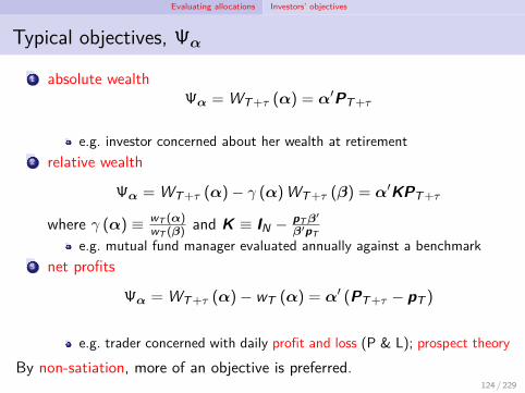
Typical objectives, Ψα
1 absolute wealthΨα = WT+τ (α) = α′PT+τ
e.g. investor concerned about her wealth at retirement2 relative wealth
Ψα = WT+τ (α)− γ (α)WT+τ (β) = α′KPT+τ
where γ (α) ≡ wT (α)wT (β) and K ≡ IN − pTβ
′
β′pTe.g. mutual fund manager evaluated annually against a benchmark
3 net profits
Ψα = WT+τ (α)− wT (α) = α′ (PT+τ − pT )
e.g. trader concerned with daily profit and loss (P & L); prospect theory
By non-satiation, more of an objective is preferred.124 / 229
Evaluating allocations Investors’ objectives
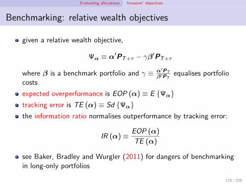
Benchmarking: relative wealth objectives
given a relative wealth objective,
Ψα ≡ α′PT+τ − γβ′PT+τ
where β is a benchmark portfolio and γ ≡ α′PTβ′PT
equalises portfoliocostsexpected overperformance is EOP (α) ≡ E Ψαtracking error is TE (α) ≡ Sd Ψαthe information ratio normalises outperformance by tracking error:
IR (α) ≡ EOP (α)
TE (α)
see Baker, Bradley and Wurgler (2011) for dangers of benchmarkingin long-only portfolios
125 / 229

Evaluating allocations Investors’ objectives
Objectives, in general
in all the objectives considered
Ψα = α′M
where M ≡ a + BPT+τ is the market vector, the relevant affinetransformation of horizon prices, and B is invertible(what are a and B for the previous examples?)the distribution of M is easily computed from that of PT+τ
ϕM (ω) ≡E
eiω′M= E
eiω′(a+BPT+τ )
= E
eiω′aeiω′BPT+τ
=eiω′aϕPT+τ
(B′ω
)can easily show that Ψα is
1 homogeneous of degree one: Ψλα = λΨα
2 additive: Ψα+β = Ψα +Ψβ
as objective is a rv, how compare two portfolios, α and β?126 / 229
Evaluating allocations Stochastic dominance
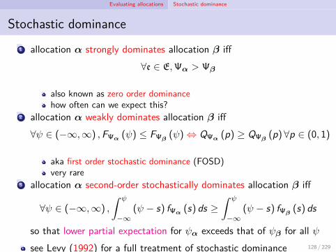
Stochastic dominance1 allocation α strongly dominates allocation β iff
∀e ∈ E,Ψα > Ψβ
also known as zero order dominancehow often can we expect this?
2 allocation α weakly dominates allocation β iff∀ψ ∈ (−∞,∞) ,FΨα (ψ) ≤ FΨβ
(ψ) ⇔ QΨα (p) ≥ QΨβ(p) ∀p ∈ (0, 1)
aka first order stochastic dominance (FOSD)very rare
3 allocation α second-order stochastically dominates allocation β iff
∀ψ ∈ (−∞,∞) ,
∫ ψ
−∞(ψ − s) fΨα (s) ds ≥
∫ ψ
−∞(ψ − s) fΨβ
(s) ds
so that lower partial expectation for ψα exceeds that of ψβ for all ψsee Levy (1992) for a full treatment of stochastic dominance 128 / 229
Evaluating allocations Measures of satisfaction
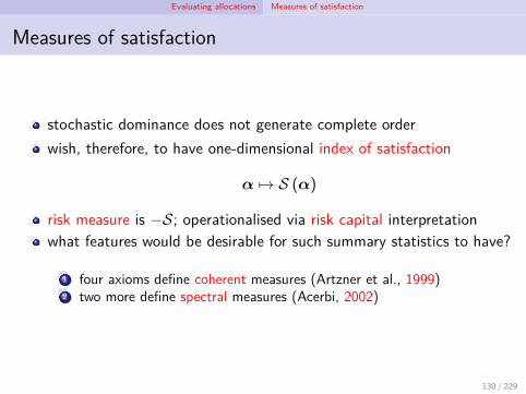
Measures of satisfaction
stochastic dominance does not generate complete orderwish, therefore, to have one-dimensional index of satisfaction
α 7→ S (α)
risk measure is −S; operationalised via risk capital interpretationwhat features would be desirable for such summary statistics to have?
1 four axioms define coherent measures (Artzner et al., 1999)2 two more define spectral measures (Acerbi, 2002)
130 / 229

Evaluating allocations Measures of satisfaction
Coherence axiom 1: translation invariance
if allocation b yields deterministic, ψb translation invariance requires
S (α+ b) = S (α) + S (b) = S (α) + ψb
this, in turn, implies1 constancy: α = 0 ⇒ S (α) = ψα = 0, so that S (b) = ψb (satisfaction
of the deterministic outcome is the outcome itself)2 if unit of measurement is money, money-equivalence: receiving extra
£1mn increases satisfaction (resp decreases risk capital) by £1mnn.b. additive objectives do not imply additive satisfaction:
Ψα+β = Ψα +Ψβ ⇒ S (α+ β) = S (α) + S (β)
certainty-equivalence quantile coherent indices expected shortfall
131 / 229

Evaluating allocations Measures of satisfaction
Money-equivalence v scale-invariance
Example1 expected value: S (α) = E Ψα2 Sharpe ratio: SR (α) = EΨα
SdΨαWhen have we seen a Sharpe ratio previously?
which of the above are money-equivalent?by contrast, dimensionless scale-invariance (homogeneity of degreezero)
S (λα) = S (α)∀λ > 0
normalises size of portfolio awaywhich of the above are scale-invariant?
certainty-equivalence quantile expected shortfall
132 / 229

Evaluating allocations Measures of satisfaction
Coherence axiom 2: super-additivity
an index of satisfaction is super-additive if two portfolios yield a higherindex of satisfaction than the indices of the portfolios individually
S (α+ β) ≥ S (α) + S (β)
this is desirable as the summed portfolio is at least as diversified asthe individual portfoliossuper-additive satisfaction measure implies what sort of risk measure?
certainty-equivalence quantile coherent indices expected shortfall
Example (Expected value)S (α+ β) ≡ E Ψα+β = E Ψα+ E Ψβ = S (α) + S (β)
133 / 229
Evaluating allocations Measures of satisfaction
Coherence axiom 3: positive homogeneity
we know rescaling an allocation rescales the objective identically
Ψλα = λΨα∀λ ≥ 0
if an index of satisfaction rescales similarly, it is homogeneous withdegree one or positive homogenous
S (λα) = λS (α) ∀λ ≥ 0
Euler’s homogeneous function theorem allows satisfaction to bedecomposed into hotspots, contributions from each security
S (α) =N∑
n=1αn∂S (α)
∂αn
certainty-equivalence quantile coherent indices expected shortfall
134 / 229
Evaluating allocations Measures of satisfaction
Positive homogeneity + super-additivity ⇒ concavity
an index of satisfaction is concave iff
S (λα+ (1 − λ)β) ≥ λS (α) + (1 − λ)S (β) ∀λ ∈ [0, 1]
relevance: diversification via convex combinations of two portfolios(e.g. budget constrained) increase satisfactionpositive homogeneity and super-additivity imply concavity (resp.convexity for risk measures)
S (λα+ (1 − λ)β) ≥S (λα) + S ((1 − λ)β)
=λS (α) + (1 − λ)S (β)
by super-additivity, positive homogeneity respectivelycertainty-equivalence quantile expected shortfall
135 / 229
Evaluating allocations Measures of satisfaction
Coherence axiom 4: monotonicity
by non-satiation, a satisfaction index satisfies monotonicity iff
Ψα ≥ Ψβ∀e ∈ E ⇒ S (α) ≥ S (β)
thus, monotonicity requires consistency with strong dominanceα strongly dominates β ⇒ S (α) ≥ S (β)
again, seems a sensible requirement
Counterexample: 2006 Swiss Solvency Test (SST)a framework for determining “the solvency capital required for aninsurance company . . . There are situations where the company is allowedto give away a profitable non-risky part of its asset-liability portfolio whilereducing its target capital.” (Filipovi and Vogelpoth, 2008)Reduces Ψα to Ψβ ≤ Ψα, but −S (β) ≤ −S (α) ⇔ R (β) ≤ R (α).
certainty-equivalence quantile coherent indices expected shortfall
136 / 229
Evaluating allocations Measures of satisfaction
Spectral axiom 5: law invariance
law invariant: S depends only on distribution of Ψα (e.g.fΨα ,FΨα , ϕΨα ,QΨα)equivalent to estimable from empirical data: by Glivenko-Cantelli, assamples become large, identically distributed rvs yield the same S
Counterexample: general equilibrium measures of risk“the risk of a portfolio depends on the other assets . . . in the eco-nomy (the market portfolio) . . . The corresponding measure of riskof a portfolio [is the] cash needed to sell the risk . . . in the portfolioto the market” (Csóka, Herings and Kóczy, 2007)
Market impact: thin markets (illiquid or emerging) or correlated behaviour(Shin, 2010), inc. algorithmic crowdingWorst conditional expectation (Artzner et al., 1999, Definition 5.2) notlaw invariant as conditions on state space (Acerbi, 2002)Hanson, Kashyap and Stein (2011) on macroprudential regulation
certainty-equivalence quantile expected shortfall137 / 229

Evaluating allocations Measures of satisfaction
Spectral axiom 6: co-monotonic additivity
allocations α and δ are co-monotonic if their objectives areco-monotonic co-monotonicity
combining co-monotonic allocations does not provide genuinediversificationthus, index of satisfaction is co-monotonically additive iff
(α, δ) co-monotonic ⇒ S (α+ δ) = S (α) + S (δ)
such indices are “derivative-proof”certainty-equivalence quantile expected shortfall
138 / 229
Evaluating allocations Measures of satisfaction
law invariant + monotonic ⇒ consistent with stochasticdominance
have applied non-satiation to stochastic dominance: can also apply toweaker concepts of dominancespectral measure ⇒ consistence with weak / first order dominance
QΨα (p) ≥ QΨβ(p) ∀p ∈ (0, 1) ⇒ S (α) ≥ S (β)
(Meucci, 2005, p.291,www.5.2)monotonicity’s Ψα ≥ Ψβ∀e ∈ E is stronger than FOSD’sFΨα (ψ) ≤ FΨβ
(ψ)∀ψ ∈ R; law invariance prevents any other factorscertainty-equivalence quantile expected shortfall
139 / 229
Evaluating allocations Measures of satisfaction
Desideratum: risk-aversion
let b be an allocation yielding a deterministic objective, ψblet f be a ‘fair game’ allocation whose objective has E Ψf = 0an index of satisfaction displays risk-aversion iff
S (b) ≥ S (b + f )the risk-premium is the dissatisfaction associated with the risky f
RP ≡ S (b)− S (b + f )(if money-equivalent, how interpret?)if S satisfies constancy, and E Ψα exists, can factor intodeterministic and ‘fair game’ components
RP (α) ≡ E Ψα − S (α)
(why?)risk-aversion ⇔ RP (α) ≥ 0(relationship to concavity?)
certainty-equivalence quantile expected shortfall140 / 229

Evaluating allocations Measures of satisfaction
Lecture 7 exercises
Meucci exercisespencil-and-paper: 7.2.1, 7.2.2, 7.3.2 (how do we “notice that normalmarginals [bound together by] a normal copula give rise to a normaljoint distribution”?), 7.3.3Python: 7.1.1 (why is equation 440 not a typo?)
project: given your assets, write code to calculate its net profits
141 / 229

Evaluating allocations Certainty-equivalent (expected utility)
Expected utility
recall, a measure of satisfaction maps from an allocation to a number:α 7→ S (α)
utility function associated with each realisation, ψ, some utility, u (ψ)
expected utility is therefore
α 7→ E u (Ψα) ≡∫R
u (ψ) fΨα (ψ) dψ
(why not just use the expected value of the objective, E Ψα?)as utility has no meaningful units, invert to obtain certainty-equivalent
α 7→ CE (α) ≡ u−1 (E u (Ψα))
143 / 229
Evaluating allocations Certainty-equivalent (expected utility)
Properties of certainty-equivalence
1 translation invariance? translation invariance
only for u (ψ) = −e−1ζψ (Meucci, 2005, www.5.3)
2 super-additivity? super-additivity
(Meucci, 2005, p.267): only holds for linear utility, u (ψ) ≡ ψ(what do Hennessy and Lapan (2006) results say?)
3 positive homogeneity? positive homogeneity
only for u (ψ) = ψ1− 1γ , γ ≥ 1 ⇒ (Meucci, 2005, www.5.3)
4 monotonicity? monotonicity
what condition is required?5 law-invariance? law-invariance
6 co-monotonic additivity? co-monotonic additivity
(Meucci, 2005, p.267): only holds for linear utility, u (ψ) ≡ ψ
144 / 229
Evaluating allocations Certainty-equivalent (expected utility)
Properties of certainty-equivalence
7 concavity? concavity
as sum of concave functions is concave, E u (·) concave if u (·) isbut this implies that u−1 is convex, so u−1 (E u (·)) needn’t be
8 risk-aversion? risk-aversion
as CE satisfies constancy
RP (α) ≡ E Ψα − CE (α)
u (·) concave ⇔ RP (α) ≥ 0 (Meucci, 2005, www.5.3)
145 / 229

Evaluating allocations Certainty-equivalent (expected utility)
Computing CE (α) ≡ u−1 (E u (α′M))
Example (Exponential utility; normally distributed markets)
exponential utility: u (ψ) ≡ −e−1ζψ ⇒ CE (α) = −ζ ln
(ϕM
(iζα))
normally distributed markets:M ∼ N (µ,Σ) ⇒ CE (α) = α′µ− α′Σα
2ζ
usually must approximate, e.g. second-order Taylor series expansion
CE (α) ≡ E Ψα − RP (α) ≈ E Ψα −12A (E Ψα)Var Ψα
where A (ψ) ≡ −u′′(ψ)u′(ψ) is the Arrow-Pratt measure of absolute
risk-aversion
146 / 229

Evaluating allocations Quantile (Value at Risk)
Introduction to VaR
how much can we lose on our trading portfolio by tomorrow’sclose? (Attributed to Dennis Weatherstone, motivating his famous4:15 reports (Allen, Boudoukh and Saunders, 2004))
given an investment horizon, and a confidence level, c, VaR is themaximum loss over that period c% of the timepopularity grew after 1996, when J.P. Morgan published its VaRmethodologyin 1998, J.P. Morgan spun off the RiskMetrics grouppreferred measure of market risk adopted since Basel IIcan control bankruptcy risk (Shin, 2010)credit risk version called potential future exposure
148 / 229
Evaluating allocations Quantile (Value at Risk)
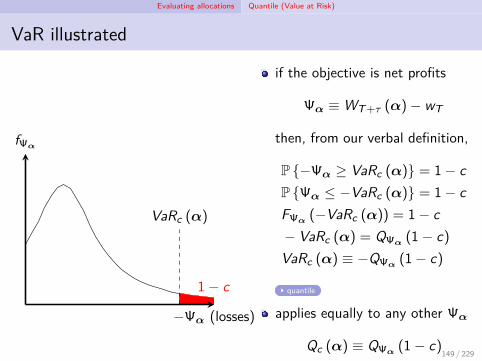
VaR illustrated
1 − c
VaRc (α)
−Ψα (losses)
fΨα
if the objective is net profits
Ψα ≡ WT+τ (α)− wT
then, from our verbal definition,
P −Ψα ≥ VaRc (α) = 1 − cP Ψα ≤ −VaRc (α) = 1 − cFΨα (−VaRc (α)) = 1 − c− VaRc (α) = QΨα (1 − c)VaRc (α) ≡ −QΨα (1 − c)
quantile
applies equally to any other Ψα
Qc (α) ≡ QΨα (1 − c)
(why no negative sign?)
149 / 229
Evaluating allocations Quantile (Value at Risk)
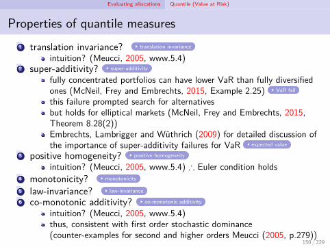
Properties of quantile measures1 translation invariance? translation invariance
intuition? (Meucci, 2005, www.5.4)2 super-additivity? super-additivity
fully concentrated portfolios can have lower VaR than fully diversifiedones (McNeil, Frey and Embrechts, 2015, Example 2.25) VaR fail
this failure prompted search for alternativesbut holds for elliptical markets (McNeil, Frey and Embrechts, 2015,Theorem 8.28(2))Embrechts, Lambrigger and Wüthrich (2009) for detailed discussion ofthe importance of super-additivity failures for VaR expected value
3 positive homogeneity? positive homogeneity
intuition? (Meucci, 2005, www.5.4) ∴ Euler condition holds4 monotonicity? monotonicity
5 law-invariance? law-invariance
6 co-monotonic additivity? co-monotonic additivity
intuition? (Meucci, 2005, www.5.4)thus, consistent with first order stochastic dominance(counter-examples for second and higher orders Meucci (2005, p.279))
150 / 229

Evaluating allocations Quantile (Value at Risk)
Properties of quantile measures
7 concavity? concavity
failure related to that of super-additivity, above?8 risk-aversion? risk-aversion
RP (α) can take on any sign
151 / 229
Evaluating allocations Quantile (Value at Risk)
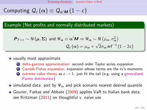
Computing Qc (α) ≡ Qα′M (1 − c)
Example (Net profits and normally distributed markets)
PT+τ ∼ N (µ,Σ) and Ψα ≡ α′M ⇒ Ψα ∼ N(µα, σ
2α
)Qc (α) = µα +
√2σα erf−1 (1 − 2c)
usually must approximate1 delta-gamma approximation: second order Taylor series expansion2 Cornish-Fisher expansion: expansion whose terms are the rv’s moments3 extreme value theory as c → 1: just fit the tail (e.g. using a generalised
Pareto distribution)simulated data: sort by Ψα and pick scenario nearest desired quantileGourier, Farkas and Abbate (2009) applies VaR to Italian bank data;see Kritzman (2011) on thoughtful v. naïve use
152 / 229
Evaluating allocations Coherent indices of satisfaction
Spectral indices (Acerbi, 2002)
existing indices either satisfied or failed to satisfy certain propertiesboth expected utility (in general) and quantile measures fail to satisfysuper-additivity, concavityboth may therefore fail to understand motives for diversificationcoherent indices designed to satisfy these propertiesgiven a coherent index, how can others be generated?question gave rise to spectral indices, a subclass of coherent indices
in satisfying additional two axioms, also satisfy risk-aversion
154 / 229
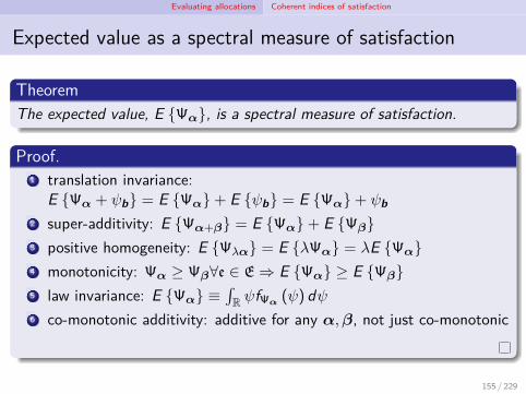
Evaluating allocations Coherent indices of satisfaction
Expected value as a spectral measure of satisfaction
TheoremThe expected value, E Ψα, is a spectral measure of satisfaction.
Proof.1 translation invariance:
E Ψα + ψb = E Ψα+ E ψb = E Ψα+ ψb2 super-additivity: E Ψα+β = E Ψα+ E Ψβ3 positive homogeneity: E Ψλα = E λΨα = λE Ψα4 monotonicity: Ψα ≥ Ψβ∀e ∈ E ⇒ E Ψα ≥ E Ψβ5 law invariance: E Ψα ≡
∫R ψfΨα (ψ) dψ
6 co-monotonic additivity: additive for any α,β, not just co-monotonic
155 / 229
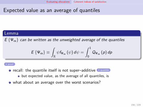
Evaluating allocations Coherent indices of satisfaction
Expected value as an average of quantiles
LemmaE Ψα can be written as the unweighted average of the quantiles
E Ψα ≡∫RψfΨα (ψ) dψ =
∫ 1
0QΨα (p) dp
proof
recall: the quantile itself is not super–additive quantile
but expected value, as the average of all quantiles, iswhat about an average over the worst scenarios?
156 / 229
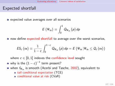
Evaluating allocations Coherent indices of satisfaction
Expected shortfall
expected value averages over all scenarios
E Ψα ≡∫ 1
0QΨα (p) dp
now define expected shortfall to average over the worst scenarios,
ESc α ≡ 11 − c
∫ 1−c
0QΨα (p) dp = E Ψα |Ψα ≤ Qc (α)
where c ∈ [0, 1] indexes the confidence level soughtwhy is the (1 − c)−1 term present?when fΨα is smooth (Acerbi and Tasche, 2002), equivalent to
tail conditional expectation (TCE)conditional value at risk (CVaR)
157 / 229

Evaluating allocations Coherent indices of satisfaction
Properties of expected shortfall
1 translation invariance? translation invariance
from linearity of integral and translation invariance of quantile2 super-additivity? super-additivity
as averaging over tail, can’t ‘bomb’ it as can VaRsee Acerbi and Tasche (2002, Proposition A.1)
3 positive homogeneity? positive homogeneity
integral is linear; quantile is positively homogeneous; again, Eulercondition holds
4 monotonicity? monotonicity
5 law-invariance? law-invariance
6 co-monotonic additivity? co-monotonic additivity
from linearity of integral and co-monotonic additivity of quantile
158 / 229
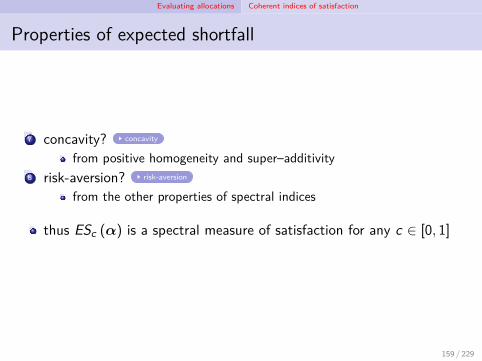
Evaluating allocations Coherent indices of satisfaction
Properties of expected shortfall
7 concavity? concavity
from positive homogeneity and super–additivity8 risk-aversion? risk-aversion
from the other properties of spectral indices
thus ESc (α) is a spectral measure of satisfaction for any c ∈ [0, 1]
159 / 229
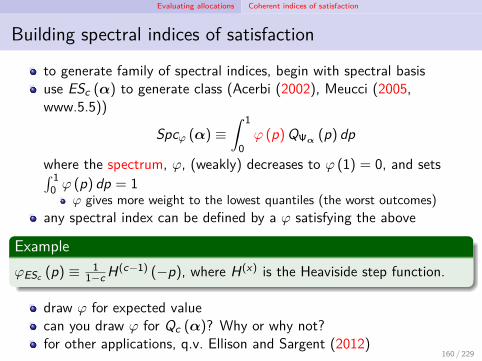
Evaluating allocations Coherent indices of satisfaction
Building spectral indices of satisfaction
to generate family of spectral indices, begin with spectral basisuse ESc (α) to generate class (Acerbi (2002), Meucci (2005,www.5.5))
Spcφ (α) ≡∫ 1
0φ (p)QΨα (p) dp
where the spectrum, φ, (weakly) decreases to φ (1) = 0, and sets∫ 10 φ (p) dp = 1
φ gives more weight to the lowest quantiles (the worst outcomes)any spectral index can be defined by a φ satisfying the above
ExampleφESc (p) ≡ 1
1−c H(c−1) (−p), where H(x) is the Heaviside step function.
draw φ for expected valuecan you draw φ for Qc (α)? Why or why not?for other applications, q.v. Ellison and Sargent (2012)
160 / 229

Evaluating allocations Coherent indices of satisfaction
Computing Spcφ (α) ≡∫ 1
0 φ (p)Qα′M (p) dp
Example (Net profits and normally distributed markets)
PT+τ ∼ N (µ,Σ) and Ψα ≡ α′M ⇒ Ψα ∼ N(µα, σ
2α
)Qα′M (α) = µα +
√2σα erf−1 (1 − 2c)
⇒ Spcα = µα +√
2σα∫ 1
0φ (p) erf−1 (2p − 1) dp
usually approximate, e.g. delta-gamma approximation orCornish-Fisher expansionfor ESc (α), can also use extreme value theory as c → 1simulated data: sort by Ψα and average scenarios below Qc (α)
161 / 229
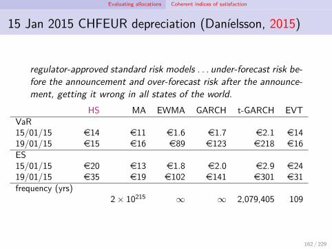
Evaluating allocations Coherent indices of satisfaction
15 Jan 2015 CHFEUR depreciation (Daníelsson, 2015)
regulator-approved standard risk models . . . under-forecast risk be-fore the announcement and over-forecast risk after the announce-ment, getting it wrong in all states of the world.
HS MA EWMA GARCH t-GARCH EVTVaR15/01/15 e14 e11 e1.6 e1.7 e2.1 e1419/01/15 e15 e16 e89 e123 e218 e16ES15/01/15 e20 e13 e1.8 e2.0 e2.9 e2419/01/15 e35 e19 e102 e141 e301 e31frequency (yrs)
2 × 10215 ∞ ∞ 2,079,405 109
162 / 229

Evaluating allocations Coherent indices of satisfaction
Lecture 8 exercises
Meucci exercisespencil-and-paper: 7.4.1, 7.5.1 (not Python)Python: 7.4.1, 7.4.2, 7.4.3, 7.5.1 (Python), 7.5.2
project: given your assets and a one hour horizon, calculate the 1%VaR
163 / 229
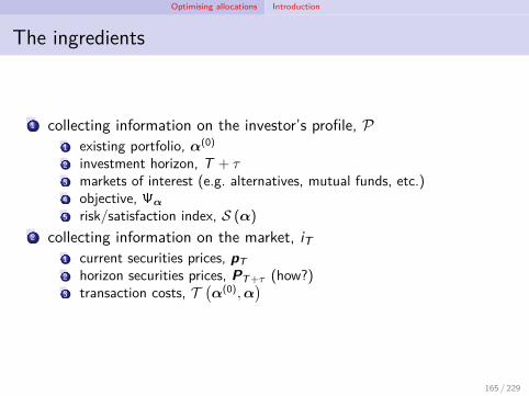
Optimising allocations Introduction
The ingredients
1 collecting information on the investor’s profile, P1 existing portfolio, α(0)
2 investment horizon, T + τ3 markets of interest (e.g. alternatives, mutual funds, etc.)4 objective, Ψα
5 risk/satisfaction index, S (α)
2 collecting information on the market, iT1 current securities prices, pT2 horizon securities prices, PT+τ (how?)3 transaction costs, T
(α(0),α
)
165 / 229
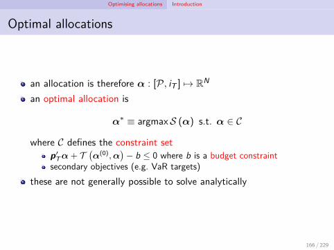
Optimising allocations Introduction
Optimal allocations
an allocation is therefore α : [P, iT ] 7→ RN
an optimal allocation is
α∗ ≡ argmaxS (α) s.t. α ∈ C
where C defines the constraint setp′
Tα+ T(α(0),α
)− b ≤ 0 where b is a budget constraint
secondary objectives (e.g. VaR targets)these are not generally possible to solve analytically
166 / 229
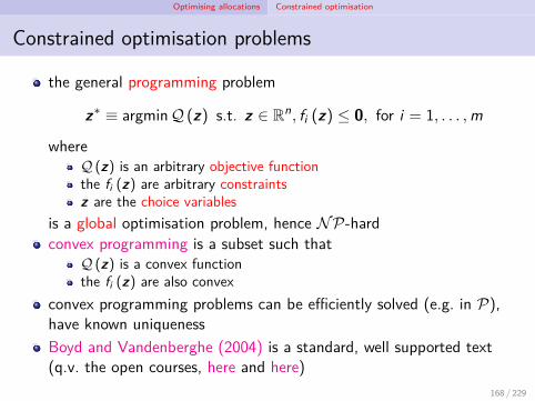
Optimising allocations Constrained optimisation
Constrained optimisation problems
the general programming problem
z∗ ≡ argminQ (z) s.t. z ∈ Rn, fi (z) ≤ 0, for i = 1, . . . ,m
whereQ (z) is an arbitrary objective functionthe fi (z) are arbitrary constraintsz are the choice variables
is a global optimisation problem, hence NP-hardconvex programming is a subset such that
Q (z) is a convex functionthe fi (z) are also convex
convex programming problems can be efficiently solved (e.g. in P),have known uniquenessBoyd and Vandenberghe (2004) is a standard, well supported text(q.v. the open courses, here and here)
168 / 229
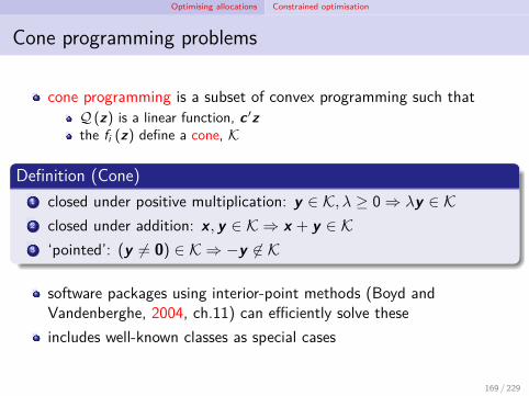
Optimising allocations Constrained optimisation
Cone programming problems
cone programming is a subset of convex programming such thatQ (z) is a linear function, c ′zthe fi (z) define a cone, K
Definition (Cone)1 closed under positive multiplication: y ∈ K, λ ≥ 0 ⇒ λy ∈ K2 closed under addition: x, y ∈ K ⇒ x + y ∈ K3 ‘pointed’: (y = 0) ∈ K ⇒ −y ∈ K
software packages using interior-point methods (Boyd andVandenberghe, 2004, ch.11) can efficiently solve theseincludes well-known classes as special cases
169 / 229
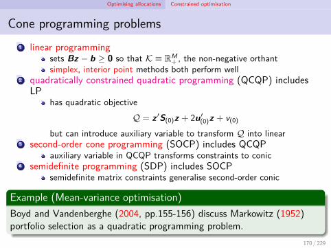
Optimising allocations Constrained optimisation
Cone programming problems1 linear programming
sets Bz − b ≥ 0 so that K ≡ RM+ , the non-negative orthant
simplex, interior point methods both perform well2 quadratically constrained quadratic programming (QCQP) includes
LPhas quadratic objective
Q = z ′S(0)z + 2u′(0)z + v(0)
but can introduce auxiliary variable to transform Q into linear3 second-order cone programming (SOCP) includes QCQP
auxiliary variable in QCQP transforms constraints to conic4 semidefinite programming (SDP) includes SOCP
semidefinite matrix constraints generalise second-order conic
Example (Mean-variance optimisation)Boyd and Vandenberghe (2004, pp.155-156) discuss Markowitz (1952)portfolio selection as a quadratic programming problem.
170 / 229
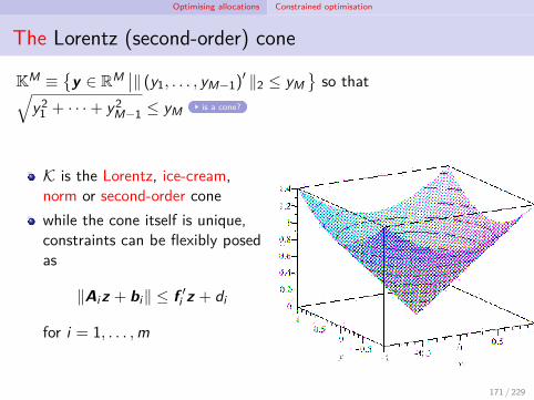
Optimising allocations Constrained optimisation
The Lorentz (second-order) cone
KM ≡
y ∈ RM ∣∣∥ (y1, . . . , yM−1)′ ∥2 ≤ yM
so that√
y21 + · · ·+ y2
M−1 ≤ yM is a cone?
K is the Lorentz, ice-cream,norm or second-order conewhile the cone itself is unique,constraints can be flexibly posedas
∥Aiz + bi∥ ≤ f ′i z + di
for i = 1, . . . ,m
171 / 229
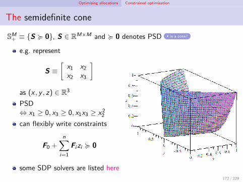
Optimising allocations Constrained optimisation
The semidefinite cone
SM+ ≡ S ≽ 0, S ∈ RM×M and ≽ 0 denotes PSD is a cone?
e.g. represent
S ≡[
x1 x2x2 x3
]as (x , y , z) ∈ R3
PSD⇔ x1 ≥ 0, x3 ≥ 0, x1x3 ≥ x2
2can flexibly write constraints
F0 +n∑
i=1Fizi ≽ 0
some SDP solvers are listed here172 / 229
Optimising allocations The mean-variance approach
The mean-variance approach
Meucci (2005, §6.1) contains perhaps only non–trivial portfoliooptimisation example that can be analytically solvedmore generally, even numerical solutions cannot be guaranteedoutside of convex programming
S or constraints are not concavequantile or certainty equivalent fail; spectral pass
even when the problem is one of a convex programming, thecomputational cost may be prohibitivehere, present mean–variance approach
use dates back to Markowitz (1952)extremely popularcomputationally tractable
174 / 229

Optimising allocations The mean-variance approach
The geometry of allocation optimisation
the indices of satisfaction considered here are law invariantthus, they can be represented in terms of the distribution of Ψαdistribution of Ψα, in turn, can be represented in terms of moments
certainty equivalent: Taylor expanding u (·) yields momentsquantiles or spectral indices: Cornish-Fisher expansion
therefore, if S (α) is an analytic function,
S (α) ≡ H (E Ψα ,CM2 Ψα ,CM3 Ψα , . . .)
where CMk is the kth central moment of Ψαiso-satisfaction surfaces therefore live in (∞− 1)-dimensionalsubspace of momentswithin this, though, α ∈ RN spans a subspacewithin that subspace, the constraint that α ∈ C is further restrictivesolving the problem is finding the point in that final subspacecorresponding to the highest level of satisfaction
175 / 229
Optimising allocations The mean-variance approach
Dimension reduction: the mean-variance framework
instead of the infinite-dimensional version of S (α), consider
S (α) ≈ H (E Ψα ,Var Ψα)
this would clearly be easier to solve, when the approximation is goodall S (α) considered above are consistent with stochastic dominance
given some fixed Var Ψα, higher E Ψα preferred for any Hcannot assume dual: given some fixed E Ψα, lower Var Ψαpreferred for any H?
⇒ optimal allocation α∗ belongs to 1-parameter family α (v), where
α (v) ≡ argmaxα ∈ C
Var Ψα = v
E Ψα
solution is Markowitz’ mean–variance efficient frontier176 / 229

Optimising allocations The mean-variance approach
A two-step approach to the mean-variance frontier
1 compute the mean-variance efficient frontier,
α (v) ≡ argmaxα ∈ C
Var Ψα = v
E Ψα
2 perform the one-dimensional search,
α∗ ≡ α (v∗) ≡ argmaxv≥0
S (α (v))
Ψα ≡ α′M ⇒ E Ψ = α′E M ,Var Ψ = α′Cov Mα,thus, can write first step in terms of the horizon market vector, M:
α (v) ≡ argmaxα ∈ C
α′Cov Mα = v ≥ 0
α′E M
(why do we do this?)177 / 229

Optimising allocations Analytical solutions of the mean-variance problem
A single affine constraint: allocation space
α2
αN
α1
d ′α = c
αMVαSR
ExampleC : α′pT = wT
let C be an affine constraint
C : d ′α = c
s.t. d ,E M not collinearfrontier then a semi-line on(N − 1)-d constrainttwo-fund separationtheorem: frontier is linearcombination of MV ,SRportfolios
1 why is frontier a line?2 why begin at αMV ?3 why dotted above αSR?
179 / 229
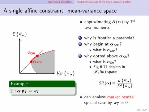
Optimising allocations Analytical solutions of the mean-variance problem
A single affine constraint: mean-variance space
αMV
αSR
E Ψα
Var Ψα
ExampleC : α′pT = wT
approximating S (α) by 1st
two moments
1 why is frontier a parabola?2 why begin at αMV ?
what is αMV ?3 why dotted above αSR?
what is αSR?Fig 6.11 depicts in(E , Sd) space
SR (α) ≡ E ΨαSd Ψα
can analyse market neutralspecial case by wT = 0
180 / 229
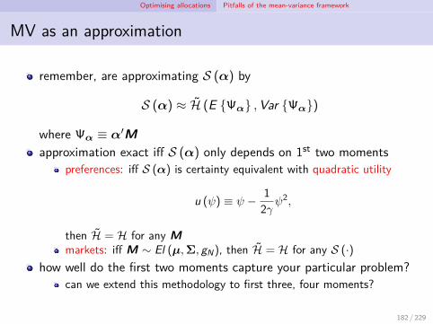
Optimising allocations Pitfalls of the mean-variance framework
MV as an approximation
remember, are approximating S (α) by
S (α) ≈ H (E Ψα ,Var Ψα)
where Ψα ≡ α′Mapproximation exact iff S (α) only depends on 1st two moments
preferences: iff S (α) is certainty equivalent with quadratic utility
u (ψ) ≡ ψ − 12γ ψ
2,
then H = H for any Mmarkets: iff M ∼ El (µ,Σ, gN), then H = H for any S (·)
how well do the first two moments capture your particular problem?can we extend this methodology to first three, four moments?
182 / 229
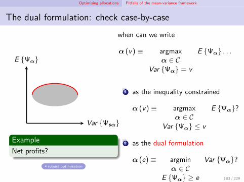
Optimising allocations Pitfalls of the mean-variance framework
The dual formulation: check case-by-case
E Ψα
Var Ψsα
ExampleNet profits?
robust optimisation
when can we write
α (v) ≡ argmaxα ∈ C
Var Ψα = v
E Ψα . . .
1 as the inequality constrained
α (v) ≡ argmaxα ∈ C
Var Ψα ≤ v
E Ψα?
2 as the dual formulation
α (e) ≡ argminα ∈ C
E Ψα ≥ e
Var Ψα?
183 / 229

Optimising allocations Pitfalls of the mean-variance framework
Lecture 9 exercises
Meucci exercisespencil-and-paper: 8.1.3 (non-Python component)Python: 8.1.1, 8.1.2, 8.1.3 (Python component), 8.1.4
project:1 for your assets (or reduced dimension version), implement the two-step
mean-variance search procedure, first identifying the locus of α (v),and then α∗
2 think about and explain why the resulting α∗ is the optimal portfolio(given a particular estimation/forecast method)
184 / 229
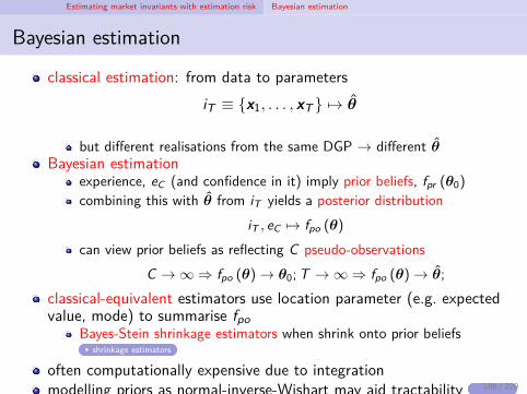
Estimating market invariants with estimation risk Bayesian estimation
Bayesian estimation
classical estimation: from data to parametersiT ≡ x1, . . . , xT 7→ θ
but different realisations from the same DGP → different θBayesian estimation
experience, eC (and confidence in it) imply prior beliefs, fpr (θ0)
combining this with θ from iT yields a posterior distributioniT , eC 7→ fpo (θ)
can view prior beliefs as reflecting C pseudo-observationsC → ∞ ⇒ fpo (θ) → θ0;T → ∞ ⇒ fpo (θ) → θ;
classical-equivalent estimators use location parameter (e.g. expectedvalue, mode) to summarise fpo
Bayes-Stein shrinkage estimators when shrink onto prior beliefsshrinkage estimators
often computationally expensive due to integrationmodelling priors as normal-inverse-Wishart may aid tractability
Wishart
186 / 229
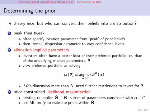
Estimating market invariants with estimation risk Determining the prior
Determining the prior
theory nice, but who can convert their beliefs into a distribution?
1 peak then tweakoften specify location parameter from ‘peak’ of prior beliefsthen ‘tweak’ dispersion parameter to vary confidence levels
2 allocation implied parametersinvestors often have a better idea of their preferred portfolio, α, thanof the underlying market parameters, θview preferred portfolio as solving
α (θ) ≡ argmaxα∈C
Sθ (α)
if θ’s dimension more than N, need further restrictions to invert for θ3 prior constrained likelihood maximisation
existing α implies Θ ⊂ Θ, subset of parameters consistent with α ∈ Cuse ML on iT to estimate priors within Θ
188 / 229

Evaluating allocations with estimation risk Allocations as decisions
Opportunity cost of suboptimal allocations
an optimal allocation solvesα∗ ≡ argmax
α∈CS (α)
the opportunity cost of a generic allocation α isOC (α) ≡ S (α∗)− S (α) ≥ 0
(for expositional clarity, ignoring costs of constraint violation)as satisfaction from any α depends on the unknown parameters
θ 7→ XθT+τ 7→ PθT+τ ⇒
(α,PθT+τ
)7→ Ψθα 7→ Sθ (α)
so does the opportunity costOCθ (α) ≡ Sθ (α∗ (θ))− Sθ (α) ≥ 0
as generic allocation depends on data, iT , so does opportunity costOCθ (α [iT ]) ≡ Sθ (α∗ (θ))− Sθ (α [iT ]) ≥ 0
but unobtainable Sθ (α∗ (θ)) does not (why?) 190 / 229
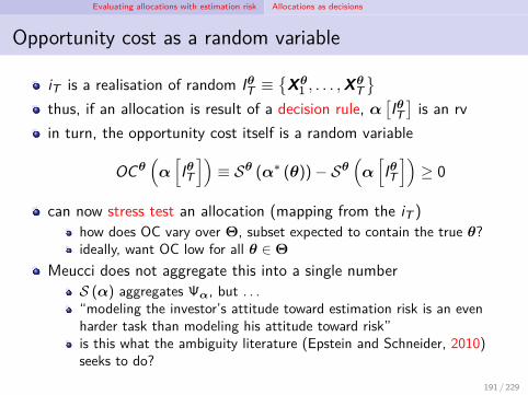
Evaluating allocations with estimation risk Allocations as decisions
Opportunity cost as a random variable
iT is a realisation of random IθT ≡
Xθ1 , . . . ,Xθ
T
thus, if an allocation is result of a decision rule, α[IθT]
is an rvin turn, the opportunity cost itself is a random variable
OCθ(α[IθT])
≡ Sθ (α∗ (θ))− Sθ(α[IθT])
≥ 0
can now stress test an allocation (mapping from the iT )how does OC vary over Θ, subset expected to contain the true θ?ideally, want OC low for all θ ∈ Θ
Meucci does not aggregate this into a single numberS (α) aggregates Ψα, but . . .“modeling the investor’s attitude toward estimation risk is an evenharder task than modeling his attitude toward risk”is this what the ambiguity literature (Epstein and Schneider, 2010)seeks to do?
191 / 229

Evaluating allocations with estimation risk Prior allocation
Allocating on the basis of priors only
consider the prior allocation rule
αp [iT ] ≡ α
where α is a fixed portfoliothen the opportunity cost becomes deterministic, given θ
OCθ(αp[IθT])
≡ Sθ (α∗ (θ))− Sθ (αp) ≥ 0
further, OCθ (αp) is generally largeq.v. bias of constant estimator
Example (Equally-weighted portfolio)The equally-weighted portfolio is determined exclusively by prior views.
193 / 229

Evaluating allocations with estimation risk Sample allocation
Sample-based allocation
until this week, have estimated parameters from data, θ [iT ]let the sample allocation be
αs [iT ] ≡ α(θ [iT ]
)≡ argmaxα∈Cθ[iT ]
S θ[iT ] (α)
to evaluate performance, do the following ∀θ ∈ Θ (the stress testset)
1 compute the deterministic Sθ (α∗ (θ))2 generate a distribution of iT ’s ⇒ distribution for θ
[IθT]
3 produce distribution of ‘optimal’ allocations, indexed by θ
αs[IθT]≡ α
(θ[IθT])
≡ argmax
α∈Cθ[IθT ]S θ[I
θT ] (α)
4 compute distribution of Sθ(αs[IθT])
, given indexed θ5 compute the distribution of
OCθ(αs[IθT])
≡ Sθ (α∗ (θ))− Sθ(αs[IθT])
thus, for each θ ∈ Θ have a distribution of OCθ(αs[IθT])
195 / 229

Evaluating allocations with estimation risk Sample allocation
Evaluating the sample-based allocation approach
if θ is an unbiased estimator of θ, then bulk of OCθ(αs[IθT])
distribution is close to zerohowever, αs is inefficient due to sensitivity of optimal allocation toinefficiency in θ
1 as sample-based estimators are inefficient, θ[IθT]
is2 inefficient estimates of θ
[IθT]
propagate estimation error into estimatesof satisfaction, S θ, the constraints, C θ, and . . .
3 the computed optimal allocation itself, αs
thus, allocations can vary greatly with the particular history usedcan trade off bias against efficiency by using shrinkage estimators
shrinkage estimators
196 / 229
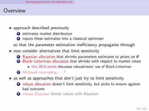
Optimising allocations with estimation risk
Overview
approach described previously1 estimates market distribution2 inputs these estimates into a classical optimiser
so that the parameter estimation inefficiency propagates throughnow consider alternatives that limit sensitivity
1 Bayesian allocation that shrinks parameters estimates to priors on θ2 Black–Litterman allocation that shrinks with respect to market views
this 2014 article discusses roboadvisors’ use of Black-Litterman3 Michaud resampling . . . ?
as well as approaches that don’t just try to limit sensitivity4 robust allocation doesn’t limit sensitivity, but picks to ensure against
bad outcome5 robust Bayesian blends robust with Bayesian
197 / 229
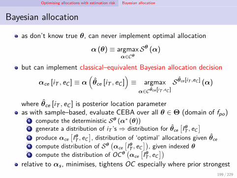
Optimising allocations with estimation risk Bayesian allocation
Bayesian allocation
as don’t know true θ, can never implement optimal allocation
α (θ) ≡ argmaxα∈Cθ
Sθ (α)
but can implement classical–equivalent Bayesian allocation decision
αce [iT , eC ] ≡ α(θce [iT , eC ]
)≡ argmaxα∈Cθce [iT ,eC ]
S θce [iT ,eC ] (α)
where θce [iT , eC ] is posterior location parameteras with sample–based, evaluate CEBA over all θ ∈ Θ (domain of fpo)
1 compute the deterministic Sθ (α∗ (θ))2 generate a distribution of iT ’s ⇒ distribution for θce
[IθT , eC
]3 produce αce
[IθT , eC
], distribution of ‘optimal’ allocations given θce
4 compute distribution of Sθ(αce
[IθT , eC
]), given indexed θ
5 compute the distribution of OCθ(αce
[IθT , eC
])relative to αs , minimises, tightens OC especially where prior strongest
199 / 229
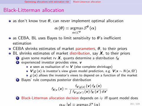
Optimising allocations with estimation risk Black-Litterman allocation
Black-Litterman allocation
as don’t know true θ, can never implement optimal allocationα (θ) ≡ argmax
α∈Cθ
Sθ (α)
as CEBA, BL uses Bayes to limit sensitivity to θ’s inefficientestimationCEBA shrinks estimates of market parameters, θ, to their priorsBL shrinks estimates of market distribution, say X , to their priors
1 given some market rv X , quants determine a distribution fX2 experienced investor provides view, v
v seen as realisation of rv V (else complete shrinkage)V |g (x) is investor’s view given model prediction, e.g. V |x ∼ N (x,Ω′)g (x) allows the investor’s views to depend on a function of the market
3 Bayes’ rule computes posterior distribution
fX|v (x) =fV |g(x) (v) fX (x)∫
fV |g(x′) (v) fX (x ′) dx ′
4 Black-Litterman allocation decision depends on iT iff quant model doesαBL [v ] ≡ argmax
α∈CvSv (α) 201 / 229

Optimising allocations with estimation risk Black-Litterman allocation
Example (Linear expertise on normal markets (Meucci, 2010))1 stock indices for Italy, Spain, Switzerland, Canada, USA, Germany are
modelled as normal, X ∼ N (µ,Σ)2 investor provides point estimates on areas of expertise, v
two views: Spanish index to gain 12% annualised, and German index tooutperform US index by 10% annualisedinvestor’s expertise is linear, g (x) = Px
P is K × N pick matrix, representing K viewsk th row is N-vector corresponding to k th viewa view on Spain, and one on US-German relative performance are
P =
(0 1 0 0 0 00 0 0 0 1 −1
)conditional distribution of views is normal,V |f (x) = V |Px ∼ N (Px,Ω)
3 the posterior market vector given the view is X |v ∼ N (µBL,ΣBL).
202 / 229

Optimising allocations with estimation risk Robust allocation
Robust allocation
now, don’t try to reduce sensitivity to inefficient estimation of θinstead, most conservative approach: minimise the maximum OCover the stress–test set
1 use iT to define robustness set, Θ [iT ], smallest Θ that contains trueθ
2 define constraint set to ensure allocation feasible for any θ ∈ Θ
CΘ[iT ] ≡α ∈ Cθ∀θ ∈ Θ [iT ]
3 the robust allocation decision then maps from iT to solve
αr [iT ] ≡ argminα∈CΘ[iT ]
max θ∈Θ[iT ]
[Sθ (α∗ (θ))− Sθ (α)
]e.g. zero-sum game against evil demon picking the worst θ ∈ Θ
205 / 229
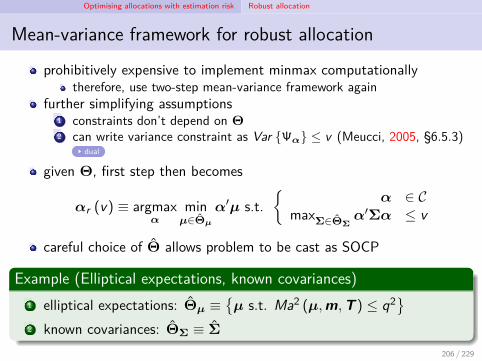
Optimising allocations with estimation risk Robust allocation
Mean-variance framework for robust allocation
prohibitively expensive to implement minmax computationallytherefore, use two-step mean-variance framework again
further simplifying assumptions1 constraints don’t depend on Θ2 can write variance constraint as Var Ψα ≤ v (Meucci, 2005, §6.5.3)
dual
given Θ, first step then becomes
αr (v) ≡ argmaxα
minµ∈Θµ
α′µ s.t.
α ∈ CmaxΣ∈ΘΣ
α′Σα ≤ v
careful choice of Θ allows problem to be cast as SOCP
Example (Elliptical expectations, known covariances)1 elliptical expectations: Θµ ≡
µ s.t. Ma2 (µ,m,T ) ≤ q2
2 known covariances: ΘΣ ≡ Σ
206 / 229
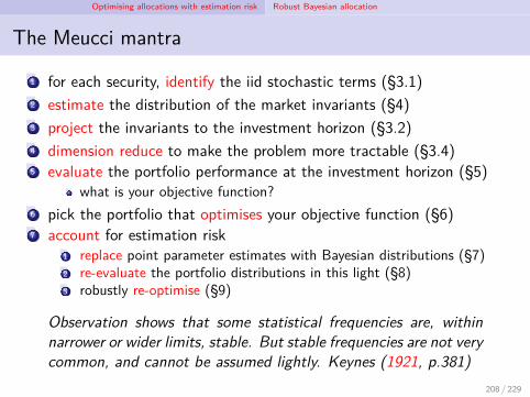
Optimising allocations with estimation risk Robust Bayesian allocation
The Meucci mantra
1 for each security, identify the iid stochastic terms (§3.1)2 estimate the distribution of the market invariants (§4)3 project the invariants to the investment horizon (§3.2)4 dimension reduce to make the problem more tractable (§3.4)5 evaluate the portfolio performance at the investment horizon (§5)
what is your objective function?6 pick the portfolio that optimises your objective function (§6)7 account for estimation risk
1 replace point parameter estimates with Bayesian distributions (§7)2 re-evaluate the portfolio distributions in this light (§8)3 robustly re-optimise (§9)
Observation shows that some statistical frequencies are, withinnarrower or wider limits, stable. But stable frequencies are not verycommon, and cannot be assumed lightly. Keynes (1921, p.381)
208 / 229

Regulatory framework of risk management
Resti and Sironi (2007, Part V) is extensive
209 / 229

Appendix References
References I
Acerbi, Carlo (2002). “Spectral measures of risk: a coherent representationof subjective risk aversion”. Journal of Banking and Finance 26.7,pp. 1505–1518.
Acerbi, Carlo and Dirk Tasche (2002). “On the coherence of expectedshortfall”. Journal of Banking and Finance 26.7, pp. 1487–1503.
Allen, Linda, Jacob Boudoukh and Anthony Saunders (2004).Understanding market, credit, and operational risk: the Value at Riskapproach. Blackwell Publishing.
Artzner, Philippe et al. (1999). “Coherent measures of risk”. MathematicalFinance 9.3, pp. 203–228.
Baker, Malcolm, Brendan Bradley and Jeffrey Wurgler (2011).“Benchmarks as limits to arbitrage: understanding the low-volatilityanomaly”. Financial Analysts Journal 67.1, pp. 40–54.
210 / 229

Appendix References
References II
Bauer, Rob and Robin Braun (2010). “Misdeeds matter: long-term stockprice performance after the filing of class-action lawsuits”. FinancialAnalysts Journal 66.6, pp. 74–92.
Berg, Christian and Christophe Vignat (2008). “Linearization coefficientsof Bessel polynomials and properties of Student t-distributions”.Constructive Approximation 27.1, pp. 15–32.
Bielecki, Tomasz R. and Marek Rutkowski (2002). Credit risk: modeling,valuation and hedging. Springer Finance. Springer.
Bookstaber, Richard (2007). A Demon of our own Design. John Wiley andSons.
Boyd, Stephen P. and Lieven Vandenberghe (2004). Convex optimization.Cambridge University Press.
Brigo, Damiano, Massimo Morini and Andrea Pallavicini (2013).Counterparty credit risk, collateral and funding. Finance. Wiley.
211 / 229

Appendix References
References III
Brock, William A. et al. (1996). “A Test for Independence Based on theCorrelation Dimension”. Econometric Reviews 15.3, pp. 197–235.
Campbell, John Y., Andrew W. Lo and A. Craig MacKinlay (1997). TheEconometrics of Financial Markets. Princeton University Press.
Cochrane, John H. (2013). “Finance: function matters, not size”. Journalof Economic Perspectives 27.2, pp. 29–50.
Csóka, Péter, P. Jean-Jacques Herings and László Á. Kóczy (2007).“Coherent measures of risk from a general equilibrium perspective”.Journal of Banking and Finance 31.8, pp. 2517–2534.
Daníelsson, Jón (2015). What the Swiss FX shock says about risk models.Tech. rep. url: http://voxeu.org/article/what-swiss-fx-shock-says-about-risk-models.
Danielsson, Jon and Jean-Pierre Zigrand (2006). “On time-scaling of riskand the square-root-of-time rule”. Journal of Banking and Finance30.10, pp. 2701–2713.
212 / 229
Appendix References
References IV
Dybvig, Philip H. and Stephen A. Ross (1985). “Differential Informationand Performance Measurement Using a Security Market Line”. Journalof Finance 40.2, pp. 383–399.
Ellison, Martin and Thomas J. Sargent (2012). “A Defence of the FOMC”.International Economic Review 53.4, pp. 1047–65.
Embrechts, Paul (2009). “Copulas: a personal view”. Journal of Risk andInsurance 76.3, pp. 639–650.
Embrechts, Paul, Dominik D. Lambrigger and Mario V. Wüthrich (2009).“Multivariate extremes and the aggregation of dependent risks:examples and counter-examples”. Extremes 12.2, pp. 107–127.
Epstein, Larry G. and Martin Schneider (2010). “Ambiguity and assetmarkets”. Annual Review of Financial Economics 2, pp. 315–346.
Fama, Eugene F. and Kenneth French (1993). “Common Risk Factors inthe Returns on Stocks and Bonds”. Journal of Financial Economics33.1, pp. 3–56.
213 / 229

Appendix References
References V
Filipovi, Damir and Nicolas Vogelpoth (2008). “A note on the SwissSolvency Test risk measure”. Insurance: Mathematics and Economics42.3, pp. 897–902.
Gordy, Michael B. (2000). “A comparative anatomy of credit risk models”.Journal of Banking and Finance 24.1–2, pp. 119–149.
Gourier, Elise, Walter Farkas and Donato Abbate (2009). “Operational riskquantification using extreme value theory and copulas: from theory topractice”. Journal of Operational Risk 4.3, pp. 1–24.
Hanson, Samuel G., Anil K. Kashyap and Jeremy C. Stein (2011). “AMacroprudential Approach to Financial Regulation”. Journal ofEconomic Perspectives 25.1, pp. 3–28.
Härdle, Wolfgang Karl and Ostap Okhrin (2010). “De copulis non estdisputandum: Colulae: an overview”. AStA Advances in StatisticalAnalysis 94.1, pp. 1–31.
214 / 229

Appendix References
References VI
Hennessy, David A. and Harvey E. Lapan (2006). “On the nature ofcertainty equivalent functionals”. Journal of Mathematical Economics43.1.
Hull, John (2009). Options, futures and other derivatives. 7th. PearsonPrentice Hall.
Hurst, Simon (1995). The characteristic function of the Student tdistribution. research report FMRR 006-95. Centre for FinancialMathematics, Australian National University.
Keynes, John Maynard (1921). A treatise on probability. London:MacMillan and Co., Ltd.
Kolanovic, Marko and Rajesh T. Krishnamachari (2017). Big Data and AIStrategies. research report. JP Morgan.
Kritzman, Mark (2011). “Long live quantitative models!” CFA InstituteMagazine, pp. 8–10.
215 / 229

Appendix References
References VII
Langetieg, Terence C., Martin L. Leibowitz and Stanley Kogelman (1990).“Duration Targeting and the Management of Multiperiod Returns”.Financial Analysts Journal 46.5, pp. 35–45.
Levy, Haim (1992). “Stochastic dominance and expected utility: surveyand analysis”. Management Science 38.4, pp. 555–593.
Malkiel, Burton G. (2003). “The Efficient Market Hypothesis and itsCritics”. Journal of Economic Perspectives 17.1, pp. 59–82.
– (2016). A random walk down Wall Street: the time-tested strategy forsuccessful investing. 11th. W.W. Norton & Co.
Markowitz, H. (1952). “Portfolio selection”. Journal of Finance 7.1,pp. 77–91.
McNeil, Alexander J., Rüdiger Frey and Paul Embrechts (2015).Quantitative Risk Management: Concepts, Techniques, and Tools.revised. Princeton Series in Finance. Princeton University Press.
216 / 229

Appendix References
References VIII
Meinhold, Richard J. and Nozer D. Singpurwalla (1983). “Understandingthe Kalman filter”. The American Statistician 37.2, pp. 123–127.
Meucci, Attilio (2005). Risk and Asset Allocation. Springer Finance.Springer.
– (2009). “Review of Discrete and Continuous Processes in Finance:Theory and Applications”. mimeo.
– (2010). “The Black-Litterman Approach: Original Model andExtensions”. mimeo.
– (2017). ARPM Lab. url: https://www.arpm.co/lab (visited on14/09/2017).
Morini, Massimo (2011). Understanding and Managing Model Risk: APractical Guide for Quants, Traders and Validators. Finance. Wiley.isbn: 978-0-470-97761-3.
Nelsen, Roger B. (2006). An Introduction to Copulas. 2nd. Springer.
217 / 229

Appendix References
References IX
Rebonato, Riccardo (2007). Plight of the Fortune Tellers: Why We Needto Manage Financial Risk Differently. Princeton University Press.
Resti, Andrea and Andrea Sironi (2007). Risk Management andShareholders’ Value in Banking. Wiley Finance. John Wiley & Sons.
Schroeder, Alice (2009). The snowball: Warren Buffett and the business oflife. Bloomsbury Publishing PLC.
Sharpe, William F. (1991). “The Arithmetic of Active Management”.Financial Analysts’ Journal 47.1, pp. 7–9.
Sherif, Nazneen (2016). “US model risk rules put lions back in theircages”. Risk.
Shin, Hyun Song (2010). Risk and liquidity. Clarendon Lectures inFinance. Oxford: Oxford University Press.
Stefanica, Dan (2011). A Primer for the Mathematics of FinancialEngineering. 2nd. Financial Engineering Advanced Background Series.New York: FE Press.
218 / 229

Appendix References
References X
Supervisory Guidance on model risk management (2011). Bulletin OCC2011-12. Board of Governors of the Federal Reserve System; and Officeof the Comptroller of the Currency.
Taylor, Stephen J., Pradeep K. Yadav and Yuanyuan Zhang (2010). “Theinformation content of implied volatilies and model-free volatilityexpectations: evidence from options written on individual stocks”.Journal of Banking and Finance 34, pp. 871–881.
219 / 229
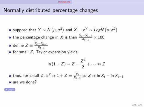
Derivations
Normally distributed percentage changes
suppose that Y ∼ N(µ, σ2) and X ≡ eY ∼ LogN
(µ, σ2)
the percentage change in X is then Xt−Xt−1Xt−1
× 100
define Z ≡ Xt−Xt−1Xt−1
for small Z , Taylor expansion yields
ln (1 + Z ) = Z − Z 2
2 + · · · ≈ Z
thus, for small Z , eZ ≈ 1 + Z = XtXt−1
so Z ≈ lnXt − lnXt−1
are we done?LogN
220 / 229
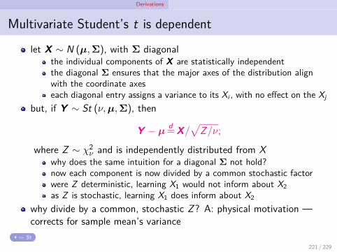
Derivations
Multivariate Student’s t is dependent
let X ∼ N (µ,Σ), with Σ diagonalthe individual components of X are statistically independentthe diagonal Σ ensures that the major axes of the distribution alignwith the coordinate axeseach diagonal entry assigns a variance to its Xi , with no effect on the Xj
but, if Y ∼ St (ν,µ,Σ), then
Y − µd=X/
√Z/ν;
where Z ∼ χ2ν and is independently distributed from X
why does the same intuition for a diagonal Σ not hold?now each component is now divided by a common stochastic factorwere Z deterministic, learning X1 would not inform about X2as Z is stochastic, learning X1 does inform about X2
why divide by a common, stochastic Z? A: physical motivation —corrects for sample mean’s variance
∼ St
221 / 229
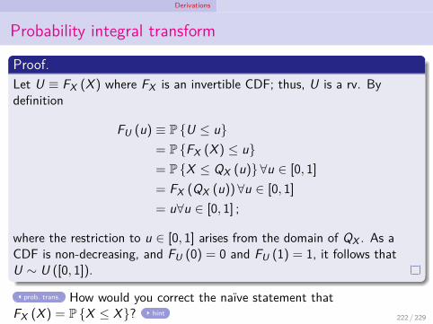
Derivations
Probability integral transform
Proof.Let U ≡ FX (X ) where FX is an invertible CDF; thus, U is a rv. Bydefinition
FU (u) ≡ P U ≤ u= P FX (X ) ≤ u= P X ≤ QX (u) ∀u ∈ [0, 1]= FX (QX (u))∀u ∈ [0, 1]= u∀u ∈ [0, 1] ;
where the restriction to u ∈ [0, 1] arises from the domain of QX . As aCDF is non-decreasing, and FU (0) = 0 and FU (1) = 1, it follows thatU ∼ U ([0, 1]).
prob. trans. How would you correct the naïve statement thatFX (X ) = P X ≤ X? hint 222 / 229

Derivations
The following proof is taken from Meucci (2005, www.3.2):
Proof.By definition of the cf, the cf of XT+τ,τ + XT+τ−τ ,τ + · · ·+ XT+τ ,τ is
ϕXT+τ,τ+XT+τ−τ ,τ+···+XT+τ ,τ(ω) = E
eiω′(XT+τ,τ+XT+τ−τ ,τ+···+XT+τ ,τ)
= E
eiω′XT+τ,τ × · · · × eiω′XT+τ ,τ
= E
eiω′XT+τ,τ
× · · · × E
eiω′XT+τ ,τ
= ϕXT+τ,τ
(ω)× · · · × ϕXT+τ ,τ(ω)
=(ϕXt,τ (ω)
) ττ
where the antepenultimate equality comes from independence, and theultimate from identicality.
223 / 229
Derivations
ATMF liquidity
futuresstandardised, exchange traded contractssettled by delivery
forwardscustomisable, OTC contractsquoted on Pink Quote, OTCBBcan be settled in cash (Stefanica, 2011, §1.10)
Bank for International Settlements: OTC market much larger thanexchange-traded (Hull, 2009, p.3)why are ATM options most liquid?
most data are ATM; anything away from that relies on assumptionsfocal point
imp vol
224 / 229
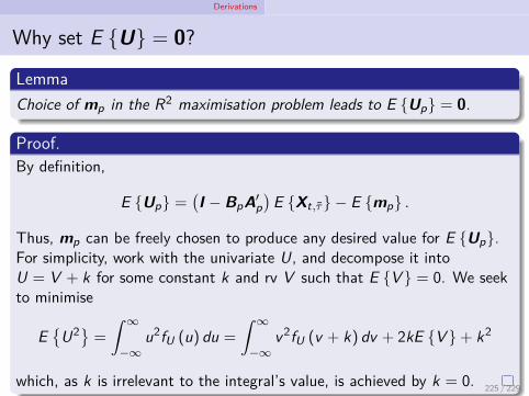
Derivations
Why set E U = 0?
LemmaChoice of mp in the R2 maximisation problem leads to E Up = 0.
Proof.By definition,
E Up =(I − BpA′
p)
E Xt,τ − E mp .
Thus, mp can be freely chosen to produce any desired value for E Up.For simplicity, work with the univariate U, and decompose it intoU = V + k for some constant k and rv V such that E V = 0. We seekto minimise
E
U2 =
∫ ∞
−∞u2fU (u) du =
∫ ∞
−∞v2fU (v + k) dv + 2kE V + k2
which, as k is irrelevant to the integral’s value, is achieved by k = 0. 225 / 229

Derivations
LemmaE Ψα can be written as the unweighted average of the quantiles
E Ψα =
∫ ∞
−∞ψfΨα (ψ) dψ =
∫ 1
0QΨα (p) dp
Proof.For any continuous g , g ′ and h, integration by substitution allows∫ b
ah (g (ψ)) g ′ (ψ) dψ =
∫ g(b)
g(a)h (p) dp
Thus, if a = −∞, b = ∞, g (·) ≡ FΨα (·), and h (·) ≡ QΨα (·):∫ ∞
−∞QΨα (FΨα (ψ)) fΨα (ψ) dψ =
∫ 1
0QΨα (p) dp
which, as QΨα and FΨα are mutual inverses, establishes the result. 226 / 229
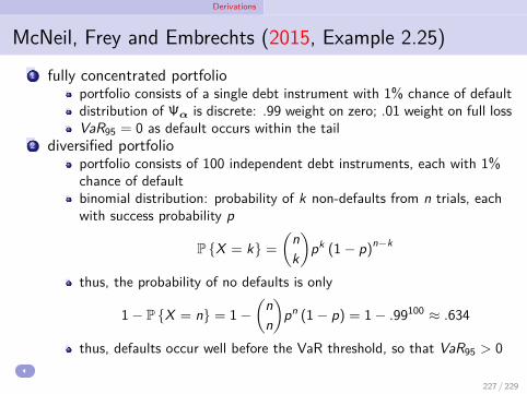
Derivations
McNeil, Frey and Embrechts (2015, Example 2.25)1 fully concentrated portfolio
portfolio consists of a single debt instrument with 1% chance of defaultdistribution of Ψα is discrete: .99 weight on zero; .01 weight on full lossVaR95 = 0 as default occurs within the tail
2 diversified portfolioportfolio consists of 100 independent debt instruments, each with 1%chance of defaultbinomial distribution: probability of k non-defaults from n trials, eachwith success probability p
P X = k =
(nk
)pk (1 − p)n−k
thus, the probability of no defaults is only
1 − P X = n = 1 −(
nn
)pn (1 − p) = 1 − .99100 ≈ .634
thus, defaults occur well before the VaR threshold, so that VaR95 > 0
227 / 229

Derivations
The Lorentz cone: KM
TheoremKM is a cone.
incomplete.1 closed under positive multiplication:2 closed under addition: by the triangular inequality for Euclidean norms
∥x−M + y−M∥ ≤ ∥x−M∥+ ∥y−M∥.
By assumption, ≤ ∥x−M∥ ≤ xM for each of x and y , so that theirsum is less than or equal to xM + yM .
3 pointed:
Lorentz cone
228 / 229
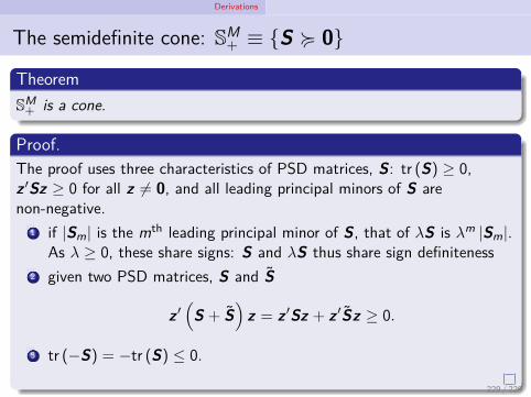
Derivations
The semidefinite cone: SM+ ≡ S ≽ 0
TheoremSM+ is a cone.
Proof.The proof uses three characteristics of PSD matrices, S: tr (S) ≥ 0,z ′Sz ≥ 0 for all z = 0, and all leading principal minors of S arenon-negative.
1 if |Sm| is the mth leading principal minor of S, that of λS is λm |Sm|.As λ ≥ 0, these share signs: S and λS thus share sign definiteness
2 given two PSD matrices, S and S
z ′(
S + S)
z = z ′Sz + z ′Sz ≥ 0.
3 tr (−S) = −tr (S) ≤ 0.
SD cone
229 / 229