RIGID-BODY DYNAMICS ALGORITHMS FOR PHYSICALLY INTERACTIVE

ROBOTS

A Thesis

Submitted to the College of Engineering

of the University of Notre Dame

in Partial Fulfillment of the Requirements

for the Degree of

Bachelors of Science

in

Mechanical Engineering

by

Sebastian F. Echeandia

Dr. Patrick M. Wensing, Advisor

Undergraduate Program in Department of Aerospace and Mechanical Engineering

Notre Dame, Indiana

April 2020

RIGID-BODY DYNAMICS ALGORITHMS FOR PHYSICALLY INTERACTIVE

ROBOTS

Abstract

by

Sebastian F. Echeandia

The development of high performance physically interactive robots has motivated

shifts in the design of actuators and novel control strategies. Mobile robots are

changing their high-impedance actuators for less stiff actuators with low gear ra-

tios. For these systems, model-based controllers have achieved unprecedented levels

of dexterity and stability compared to other control strategies. These developments

have increased the need for dynamics algorithms that can accurately compute the

dynamics of the system as part of the control policy. This work presents three new

algorithms that can be implemented in model-based controllers that require certain

dynamics terms such as the Mass or Coriolis matrices. The first objective is to exploit

a particular factorization of body-level velocity-product terms to derive an algorithm

that numerically computes the Coriolis matrix. This algorithm is of the lowest pos-

sible order, outperforming other algorithms available in the literature. The second

objective is to expand the mathematical framework to compute the Coriolis matrix to

develop an algorithm that numerically computes the corresponding Christoffel sym-

bols. Because of its low complexity, this algorithm is relevant for geometric control

schemes that do not scale based on the use of symbolic calculations. The final ob-

jective is to improve the Articulated-Body Algorithm (ABA) to take into account al

inertial effects of motor rotors by using the Gauss Principle of Least Constraints. This

Sebastian F. Echeandia

algorithm provides a more accurate alternative to other standard approximations to

include actuators’ inertial effects. Tests using simulations of different kinematic trees

show that, given their accuracy, speed, and efficiency, the three algorithms developed

in this work are viable for implementation with real-time controllers.

CONTENTS

List of Figures . . . . . . . . . . . . . . . . . . . . . . . . . . . . . . . . . . . iv

List of Tables . . . . . . . . . . . . . . . . . . . . . . . . . . . . . . . . . . . . v

Chapter 1: Introduction . . . . . . . . . . . . . . . . . . . . . . . . . . . . . . 11.1 Motivation . . . . . . . . . . . . . . . . . . . . . . . . . . . . . . . . . 11.2 Objectives . . . . . . . . . . . . . . . . . . . . . . . . . . . . . . . . . 41.3 Overview . . . . . . . . . . . . . . . . . . . . . . . . . . . . . . . . . . 6

Chapter 2: Preliminaries: Spatial Vector Notation and Rigid-Body DynamicsAlgorithms . . . . . . . . . . . . . . . . . . . . . . . . . . . . . . . . . . . 82.1 Introduction . . . . . . . . . . . . . . . . . . . . . . . . . . . . . . . . 82.2 Kinematic Tree Connectivity . . . . . . . . . . . . . . . . . . . . . . . 92.3 Spatial Vector Notation . . . . . . . . . . . . . . . . . . . . . . . . . 102.4 Equations of Motion . . . . . . . . . . . . . . . . . . . . . . . . . . . 142.5 Rigid-Body Dynamics Algorithms . . . . . . . . . . . . . . . . . . . . 16

2.5.1 Recursive Newton-Euler Algorithm . . . . . . . . . . . . . . . 162.5.2 Composite Rigid-Body Algorithm . . . . . . . . . . . . . . . . 172.5.3 Articulated-Body Algorithm . . . . . . . . . . . . . . . . . . . 18

2.6 Conclusion . . . . . . . . . . . . . . . . . . . . . . . . . . . . . . . . . 20

Chapter 3: Algorithms for the Computation of the Coriolis Matrix and Christof-fel Symbols . . . . . . . . . . . . . . . . . . . . . . . . . . . . . . . . . . . 233.1 Introduction . . . . . . . . . . . . . . . . . . . . . . . . . . . . . . . . 233.2 Algorithm Derivation . . . . . . . . . . . . . . . . . . . . . . . . . . . 23

3.2.1 Numerical Methods for Computing C . . . . . . . . . . . . . . 243.2.2 Numerical Methods for Computing Christoffel Symbols . . . . 29

3.3 Results . . . . . . . . . . . . . . . . . . . . . . . . . . . . . . . . . . . 333.3.1 Validation . . . . . . . . . . . . . . . . . . . . . . . . . . . . . 333.3.2 Performance . . . . . . . . . . . . . . . . . . . . . . . . . . . . 33

3.4 Conclusion . . . . . . . . . . . . . . . . . . . . . . . . . . . . . . . . . 37

ii

Chapter 4: Modified Articulated-Body Algorithm . . . . . . . . . . . . . . . . 394.1 Introduction . . . . . . . . . . . . . . . . . . . . . . . . . . . . . . . . 394.2 Mathematical Formalisms and Modeling Conventions . . . . . . . . . 39

4.2.1 Gauss Principle of Least Constraint . . . . . . . . . . . . . . . 394.2.2 Joint Modeling . . . . . . . . . . . . . . . . . . . . . . . . . . 40

4.3 Algorithm Derivation . . . . . . . . . . . . . . . . . . . . . . . . . . . 424.3.1 Identification of Optimization Problem . . . . . . . . . . . . . 424.3.2 Solving the Optimization Problem . . . . . . . . . . . . . . . . 444.3.3 Finding Recursive Relations . . . . . . . . . . . . . . . . . . . 464.3.4 Modified Articulated-Body Algorithm . . . . . . . . . . . . . . 48

4.4 Results . . . . . . . . . . . . . . . . . . . . . . . . . . . . . . . . . . . 484.4.1 Validation . . . . . . . . . . . . . . . . . . . . . . . . . . . . . 504.4.2 Performance . . . . . . . . . . . . . . . . . . . . . . . . . . . . 52

4.5 Conclusion . . . . . . . . . . . . . . . . . . . . . . . . . . . . . . . . . 54

Chapter 5: Conclusions . . . . . . . . . . . . . . . . . . . . . . . . . . . . . . 575.1 Summary and Conclusions . . . . . . . . . . . . . . . . . . . . . . . . 575.2 Future Work . . . . . . . . . . . . . . . . . . . . . . . . . . . . . . . . 58

Bibliography . . . . . . . . . . . . . . . . . . . . . . . . . . . . . . . . . . . . 60

iii

LIST OF FIGURES

1.1 Boston Dynamics’ quadrupeds evolution over time. . . . . . . . . . . 2

1.2 MIT Cheetah 3 climbing stairs with obstacles. . . . . . . . . . . . . . 2

2.1 A sample branched mechanism. . . . . . . . . . . . . . . . . . . . . . 10

2.2 Sample kinematic tree with body coordinate frames. . . . . . . . . . . 11

2.3 Depiction of articulated body. . . . . . . . . . . . . . . . . . . . . . . 20

3.1 Depiction of the motion of spatial joint axes due to the joint velocitiesof their ancestors. . . . . . . . . . . . . . . . . . . . . . . . . . . . . . 30

3.2 Performance for serial kinematic chains. . . . . . . . . . . . . . . . . 35

3.3 Performance for branching mechanism (branching factor of 2). . . . . 35

3.4 Computation cost for bipeds and quadrupeds. . . . . . . . . . . . . . 36

4.1 Visual comparison between constrained and unconstrained systems. . 41

4.2 Dissasembled joint between body p(i) and body i . . . . . . . . . . . 42

4.3 Force acting on body p(i). . . . . . . . . . . . . . . . . . . . . . . . . 47

4.4 Computation time for serial kinematic chains. . . . . . . . . . . . . . 53

4.5 Computation time for branching mechanism (branching factor of 2). . 53

iv

LIST OF TABLES

3.1 Validity Checks for Serial Kinematic Chains of 5, 10, and 15 Bodies(Maximum Error) . . . . . . . . . . . . . . . . . . . . . . . . . . . . . 34

3.2 Computation Time of Coriolis Matrix and Christoffel Symbols forCommon Rigid-Body Systems. . . . . . . . . . . . . . . . . . . . . . . 37

3.3 Runtime of Algorithms Using Symbolic Variables for Serial Chainswith 5,10, and 15 Bodies. . . . . . . . . . . . . . . . . . . . . . . . . . 38

4.1 Consistency Check for a Serial Kinematic Chains of 5, 10, and 15Bodies (Maximum Error) . . . . . . . . . . . . . . . . . . . . . . . . . 50

4.2 Maximum Difference in q for Serial Chains with 5, 10, and 15 Bodieswith Inertialess Actuators. . . . . . . . . . . . . . . . . . . . . . . 51

4.3 Maximum Difference in q for Serial Chains with 5, 10, and 15 Bodies. 52

4.4 Maximum Difference in q for Branching Mechanism with 5, 10, and15 Bodies (branching factor of 2). . . . . . . . . . . . . . . . . . . . . 54

4.5 Maximum Difference in q for Serial Chains with 5, 10, and 15 Bodieswhen q = π

2rad·s−1. . . . . . . . . . . . . . . . . . . . . . . . . . . . 55

4.6 Runtime for MABA and ABA. . . . . . . . . . . . . . . . . . . . . . . 55

v

CHAPTER 1

INTRODUCTION

1.1 Motivation

Many of the current research efforts in robotics are focusing on developing robots

that can safely navigate human environments and interact with people in everyday

places like offices and construction sites. The challenges presented in these environ-

ments, such as terrain unpredictability or human safety, have pushed researchers and

engineers to design robots with compliant actuators that can deliver high torques

while maintaining back-driveability. Boston Dynamics’ quadrupeds evolution from

Big Dog to Spot (Figure 1.1) illustrates the current trend in mobile robot design

of shifting from large, high-impedance actuators to smaller, less stiff actuators with

low gear ratios. This shift means that robots are designed with heavier motors and

lighter gearboxes. The lower impedance of new robotic actuators allows robots to

adapt to irregular terrains but also increases their energy efficiency and mechanical

performance [23]. With these new actuators, robots can perform tasks that require

accurate control of contact forces during scenarios like climbing stairs with unpre-

dictable obstacles (Figure 1.2).

These high-performance tasks require optimization of contact forces to be able to

achieve the desired dexterity and to maintain stability. Such optimization can be done

at the planning level, but also at the control level by tracking the desired planned

motion [22]. These model-based approaches to control need to consider the dynamics

of the system to select joint torques and forces that will make the system follow

1

Figure 1.1. Boston Dynamics’ quadrupeds evolution over time.

Figure 1.2. MIT Cheetah 3 climbing stairs with obstacles.

2

the desired behavior. Computing the dynamics of mobile robots can be a complex

challenge given the large number of degrees of freedom (DoFs) of the system, which

in turn increases the complexity of the equations of motion. Consequently, for these

controllers to be feasible in high-DoF robots, they need to be matched with accurate

and efficient rigid-body dynamics algorithms that can compute components of the

equations of motions of the system fast enough for a real-time controller. Given that

standard closed-loop controllers run in the order of ms, dynamics algorithms need to

run in the order of µs to feed information to the control loop on time.

Because of their low computational complexity, recursive dynamics algorithms

have had great success at numerically evaluating dynamics fast enough for model-

based controllers. Some successful strategies include using the operational-space for-

mulation of the dynamics of the system that enables decoupling task and null-space

dynamics to achieve high dynamic performance and active force control of robot ma-

nipulator systems [15, 30]. Other popular approaches for control consider forward

or inverse dynamics. In forward dynamics, the objective is to find the joint accel-

erations of the system, given external contact forces and internal forces and torques

[21]. Inverse dynamics consists of solving for the internal forces of the system given

its motion. Both of these problems can be solved using one of two main approaches:

Lagrangian mechanics [12, 18] or recursive algorithms [16].

While existing dynamics algorithms are cornerstones of state-of-the-art model-

based control strategies, certain challenges remain active topics of research. In par-

ticular, some applications of sensorless detection of faults acting on a robot require

the computation of a residual vector using the quantity of C>(q, q)q [2, 5], where the

matrix C(q, q) is a factorization of the Coriolis and centrifugal terms of the equations

of motion. In this application, and in other robot controls laws, the C matrix must

satisfy that H(q, q)− 2C(q, q) is skew-symmetric, where H(q) is the joint-space in-

ertia matrix. Given the transpose in C, traditional Newton-Euler algorithms cannot

3

compute this residual vector. Similarly, research efforts in the area of gradient-based

motion optimization are exploring computing components of the equations of motion,

such as C, to support optimization methods that require the calculation of partial

derivatives of the dynamics [3, 13, 14, 17, 26, 27]. For moderately complex systems,

these partial derivatives become prohibitively complex to be computed exactly, so

they are often approximated when feeding this information into the control system.

These two examples showcase that the improvement of existing recursive algo-

rithms and the development of new dynamics algorithms not only will allow to solve

increasingly complex problems building upon forward and inverse dynamics, but will

also enable the implementation of new and better control schemes. As model-based

controllers evolve, efficient and accurate dynamics algorithms will continue to present

a latent need. As such, the development of these algorithms is a pursuit with the

potential to enable further progress in the broader field of robotics.

1.2 Objectives

The overarching objective of this research is to use numerical methods to derive

new rigid-body dynamics algorithms that can be implemented in model-based con-

trollers that require dynamic terms, such as H(q) and C(q, q) as part of their control

scheme. As such, for this project to be successful, the created algorithms must fulfill

three criteria for feasibility: accuracy, speed, and efficiency. The algorithms devel-

oped in this work must equal, if not exceed, the accuracy and precision offered by

other computational methods available in the literature. Similarly, the algorithms

must be fast enough to run in a real-time control loop. The target runtime for each

algorithm is on the order of µs for systems of a moderate number of DoFs. Finally,

for the algorithms to be efficient, they must be of the lowest possible order, which

means that the computational costs of the algorithm grow proportionally with the

lowest possible power of the DoF of the system. These three criteria will ensure that

4

new algorithms are viable candidates for implementation in online controllers.

The first objective of this thesis is to exploit the link between the factorization

of body-level velocity-product terms in the equations of motion of a system to the

Coriolis matrix C to develop a recursive algorithm that can numerically compute C

directly from the motion of the system. The developed algorithm has a computa-

tional cost of O(Nd), where N is the number of bodies, and d is the depth of the

kinematic tree of the mechanism. This efficiency is superior to that of other methods

available in the literature that have a complexity of O(N2) [5]. This algorithm can

be implemented in applications of sensorless detection, but also in passivity-based

control, and adaptive control [25, 28].

The second objective is to take the mathematical framework developed for the new

algorithm to compute C and further expand it to develop a recursive algorithm that

numerically computes the underlying Christoffel symbols of the first kind of tree-

structured rigid-body systems. The complexity of the developed algorithm grows

as O(Nd2), which is much more efficient than the symbolic computation. Because

this algorithm does not require any symbolic partial derivatives, it is an attractive

alternative to approximation methods currently used in various robotics applications.

In particular, this algorithm might prove useful for geometric control schemes that

do not scale based on the use of symbolic calculations or in supporting trajectory

optimization packages by providing analytical second-order partial derivatives of the

inverse dynamics model.

Finally, the third objective is to improve the Articulated-Body Algorithm (ABA)

to accurately take into account the inertial effects of motor rotors. The computational

cost of the modified ABA grows as O(N) so that it matches the performance of the

regular ABA. ABA is a well-established forward dynamics algorithm to compute the

joint accelerations; however, in its traditional form, it lacks the ability to account

for the inertial effects of any component in the system other than the main bodies

5

of the kinematic tree. There are approximation techniques to account for inertial

effects of motors, but they are only valid for actuators with large gear ratios. The

Gauss principle of least constraint allows rederiving the ABA in such a way that

it fundamentally accounts for rotor inertias. As more robotic systems shift towards

lower gear ratios, it is essential to develop algorithms that can accurately solve the

complicated dynamics of robotic systems doing high-performance tasks in uncertain

environments.

1.3 Overview

Chapter 2 of this thesis provides the preliminary knowledge required for the

derivation of the algorithms presented in this work. It presents a general overview of

the spatial vector notation used to express the dynamics of rigid bodies more com-

pactly. It also presents the canonical equations of motion and explores the properties

that allow for the mathematical framework needed to derive new algorithms. Fi-

nally, it reviews three algorithms (Recursive Newton-Euler, Composite Rigid-Body,

and Articulated-Body) that set the general recursive strategies used by the algorithms

derived in this work.

Chapter 3 presents the derivation of an algorithm to compute C through a partic-

ular factorization of the equations of motion that allows for the recursive computation

of all entries in C. It also shows how, through some mathematical manipulation, the

same factorization leads to expressions that can be used to recursively compute the

Christoffel symbols without any symbolic manipulations. Chapter 4 shows how the

Gauss principle of least constraint leads to the derivation of an Articulated-Body

Algorithm that accurately accounts for rotor inertias. It then compares the results of

the new algorithm with the traditional ABA and a modified version of the Composite

Rigid-Body Algorithm that provides an approximation for the inertia effects of rotors

with large gear ratios. Finally, Chapter 5 provides concluding remarks for the work

6

shown throughout this thesis and suggests relevant future work in light of the results.

7

CHAPTER 2

PRELIMINARIES: SPATIAL VECTOR NOTATION AND RIGID-BODY

DYNAMICS ALGORITHMS

2.1 Introduction

This chapter presents the notation, conventions, and mathematical formalisms

that are the foundation for the algorithms developed in this work. In particular, this

chapter provides an overview of spatial notation and introduction to the 6D vectors

used to describe rigid-body dynamics in a compact notation. The conventions to

describe link connectivity within a kinematic tree are also presented, and will play

an important role in the derivation of the algorithms. The chapter discusses the

equations of motion for rigid-body systems and some of their relevant mathematical

properties that are exploited by the algorithms in later chapters. Finally, the chapter

concludes by presenting three algorithms whose overall structure and mechanics serve

as a basis for the new algorithms presented in Chapter 3 and Chapter 4. Three

key algorithms are summarized, namely 1) The Recursive Newton-Euler Algorithm

(RNEA) that computes the forces and torques at each joint given joint velocity and

acceleration; 2) The Composite Rigid-Body Algorithm (CRBA) that computes the

mass matrix; and 3) the Articulated-Body Algorithm (ABA) that computes the joint

acceleration given the joint configuration, velocities, forces, and torques.

8

2.2 Kinematic Tree Connectivity

Any rigid-body system can be described as a set of bodies connected by a set of

joints with up to 6 DoFs each. This work considers kinematic trees, where N denotes

the number of bodies and d the depth of the tree. Each body in the tree is assigned

a number from 1 to N , and a “body” 0 is assigned to represent a fixed inertial frame.

The numbering of the bodies is assigned such that for body i, its predecessor towards

the root of the tree, p(i), is less than i. This numbering system establishes a binary

relation between bodies denoted as � such that j � i indicates that body j is in the

path from body i to the root of the tree. Any pair of bodies i and j are related,

expressed as i ∼ j, if j � i or i � j.

This convention is best understood through an example. Consider the branched

mechanism in Figure 2.1. For i = 6 and j = 3, 3 � 6, so i and j are related. Similarly,

if i = 2 and j = 10, 2 � 10, so i and j are related. When i = 9 and j = 5, however,

neither of the two bodies is in the path to the root of each other; therefore, i and j

are not related in this case.

Given these conventions, an additional definition will aid in the development of

the algorithms in Chapter 3. For any pair of related bodies i ∼ j, the symbol dije

returns the body that is closest to the leaves of the kinematic tree. That is, dije is

defined as

dije =

i i � j

j o/w.

.

Consider mechanism in Figure 2.1 again as an example. If i = 7 and j = 3, then

dije = 7 since i � j. Similarly, when i = 9 and j = 2, dije would output 9 because

j � i. For cases when i and j are not related, say i = 4 and j = 6, dije is undefined

since neither of the bodies is an ancestor of the other, that is, is in the path to the

root of each other.

9

12 3

4 5

6

7

8

910

Figure 2.1. A sample branched mechanism.

2.3 Spatial Vector Notation

Spatial vectors are a convenient notation to express the equations of motion of

rigid-body systems in terms of vectors that live in a 6D vector space. Spatial vectors

significantly reduce the notational complexity of rigid-body dynamics expressed using

traditional 3D vectors. The reduced complexity makes the properties of components

of the equation of motion more apparent, which aids in the development of more

advanced algorithms. This section is intended as a short introduction; the interested

reader may refer to the in-depth explanation by Featherstone [8].

Consider the kinematic tree in Figure 2.2. To describe the motion of this system,

each body in the tree has attached a corresponding coordinate frame as shown at

joints 1, 2, and 3. These frames allow the motion of each body to be conveniently

described in a local basis. With this convention, the rate of change in position and

10

orientation of body i is expressed in terms of a spatial velocity vi ∈ R6 as

vi =

ωivi

, (2.1)

where ωi ∈ R3 and vi ∈ R3 are the angular velocity of body i and linear velocity

of the origin of frame i in body coordinates, respectively. Joint i connects body i

with its predecessor p(i) so that the velocity of body i is related to the velocity of its

predecessor as [4]

vi = iXp(i)vp(i) + Φiqi, (2.2)

where qi ∈ Rni represents the joint rates of joint i and ni indicates the number of

DoF of joint i. The term Φi ∈ R6×ni is a full-column-rank matrix that describes the

free modes of motion of joint i.

Figure 2.2. Sample kinematic tree with body coordinate frames.

The matrix iXp(i) ∈ R6×6 is the spatial transformation matrix that transforms the

basis of spatial vectors from that of frame p(i) into that of frame i. It is constructed

11

in terms of the vector p(i)pi ∈ R3 from the origin of p(i) to the origin of i and the

rotation matrix iRp(i) that transforms traditional 3D vectors from p(i)’s frame into

i’s. Overall the spatial transform is given by

iXp(i) =

iRp(i) 0

−iRp(i)S(p(i)pi)iRp(i),

, (2.3)

where S(p) is the skew-symmetric 3D cross product matrix defined for any 3D vector

p = [px, py, pz]T as

S(p) =

0 −pz py

pz 0 −px

−py px 0

. (2.4)

Similarly, the spatial force acting on body i, fi, is defined in terms of the 3D

torque and linear force so that

fi =

nif i

, (2.5)

where ni ∈ R3 is the moment about the origin of frame i and f i ∈ R3 is the linear

force expressed in body coordinates. The spatial force of a body is related to its

motion as [10]

fi = Iiai + vi ×∗ Iivi, (2.6)

where ai ∈ R6 represents the spatial acceleration of body i and Ii ∈ R6×6 is the spatial

inertia tensor that links the spatial velocity of body i to its spatial momentum. This

12

tensor is defined as

Ii =

I i miS(ci)

miS(ci)> mi13

, (2.7)

where mi is the mass of body i, ci is the vector to the center of mass of body

i expressed in local coordinates, 13 ∈ R3×3 is the identity matrix, and I i is the

conventional 3D rotational inertial tensor about the coordinate origin with elements

I i =

Ixx Ixy Ixz

Ixy Iyy Iyz

Ixz Iyz Izz

. (2.8)

For any spatial velocity v, the operator ×∗ : R6 × R6 → R6 is the bi-linear cross

product operator between spatial motion vectors and spatial force vectors expressed

as

v ×∗ f =

S(ω) S(v)

0 S(ω)

f . (2.9)

Physically, v ×∗ f gives the rate of change in the force vector f when moving with

velocity v.

The cross product operator between spatial motion vectors and spatial motion

vectors is defined in terms of ×∗ as (v×) = −(v×∗)>. Additionally, by swapping the

order of the products of the cross product, a new unique linear operator is denoted

so that (f×∗)v = (v×∗)f . Then, the ×∗ operator is expressed as

f×∗ =

−S(n) −S(f)

−S(f) 0

. (2.10)

13

The spatial inertia tensor is also subject to coordinate transformations using spa-

tial transforms. The tensor jIi, the spatial inertia of i expressed in body coordinates

of j, is expressed as

jIi = iX>j IiiXj. (2.11)

When used together, the quantities and equations presented in this chapter are

sufficient to describe the dynamics of a rigid body and will be the foundation to

describe the motion of a multi-body kinematic tree.

2.4 Equations of Motion

The equations of motion for a rigid-body system describe the motion of each

body in the system based on kinematic quantities as well as dynamic components

such as forces, torques, and gravity. In general, these equations can be derived for

any particular system using Newton’s second law or via Lagrangian methods. In

the robotics community, the equations of motion are often expressed in two different

formalisms: operational space and joint space. Operational space is often associated

with the position of the end-effector, while joint space is expressed in terms of the

position and orientation of joints in rigid-body systems. This thesis uses joint space

as the basis for the math needed to develop new dynamics algorithms.

The equations of motion of any rigid-body system can be expressed as [1]

H(q)q + C(q, q)q + g = τ , (2.12)

where H(q) ∈ Rn×n is the mass matrix containing inertial terms, C(q, q) ∈ Rn×n

is the Coriolis matrix containing Coriolis and centrifugal force terms, g ∈ Rn is the

gravity force, and τ ∈ Rn the generalized forces in the system. For kinematic trees, q

14

represents every joint variable in the mechanism contained as generalized coordinates

[8]. Similarly, q and q are generalized velocities and accelerations, respectively.

All terms in Eq. 2.12 are the factorization of the quantities contained in the equa-

tions of motion. H(q) and g are uniquely defined for a particular system. However,

note that C(q, q)q is a purely quadratic function of the entries of q. This property

makes C(q, q) not uniquely defined. In fact, there are an infinite number of valid

choices of C(q, q) for a particular set of equations of motion, all of which give the

same result for C(q, q)q.

The application of the principle of energy conservation to Eq. 2.12 when τ = 0

shows that all valid factorizations of C must satisfy the property that q>(H(q, q)−

2C(q, q))q = 0. Multiple control applications require the stronger property that the

Coriolis matrix satisfy H(q, q)− 2C(q, q) is skew-symmetric so that

η>[H(q, q)− 2C(q, q)

]η = 0 ∀,q, q,η ∈ Rn. (2.13)

One particular choice of C that satisfies Eq. 2.13 is given in terms of the Christoffel

symbols of the first kind. Christoffel symbols are tensor-like mathematical objects

used to describe the geometry of a metric on a manifold. In the case of rigid-body

dynamics, the mass matrix H provides a metric so that the Christoffel symbols (of

the first kind) are defined as [19]

Γijk =1

2

[∂Hij

∂qk+∂Hik

∂qj− ∂Hjk

∂qi

]. (2.14)

Then, a choice for C in terms of the Christoffel symbols is expressed as [24]

Cij =∑k

Γijk(q) qk. (2.15)

For a system with mass matrix H(q) and C(q, q) defined by Eq. 2.15, a matrix-

15

valued function C(q, q) is called an admissible factorization if for all q, q ∈ Rn,

1. C(q, q)q = C(q, q)q; and

2. H(q, q)− 2C(q, q) is skew symmetric.

Despite this definition of C being standard within the robotics community, it is

difficult to use in practice. For systems that are more than a few DoFs, symbolically

computing H and all its partial derivatives needed to compute C is prohibitively

computationally intensive. Therefore, novel methods to numerically compute C and

Γijk in an efficient manner will improve the feasibility and runtime performance of

some model-based controllers that use forms of C in their control laws.

2.5 Rigid-Body Dynamics Algorithms

The algorithms presented in subsequent chapters use techniques and frameworks

similar to those employed by popular recursive algorithms of the lowest order to

compute forward and inverse dynamics. The understanding of the mechanics of such

algorithms will allow drawing parallels between the algorithms presented in this work

and those extensively used in robotics applications.

2.5.1 Recursive Newton-Euler Algorithm

The RNEA is perhaps the most popular and widely used of the recursive dynamics

algorithms. This algorithm exploits the recursive relation of spatial velocities and

accelerations of a kinematic tree to solve the inverse dynamics problem, that is,

solving for the internal forces of the system given its motion. The velocity of body i

is related to the velocity of its predecessor by Eq. 2.2, its acceleration by

ai = iXp(i)ap(i) + Φiqi + (vi×)Φiqi, (2.16)

16

and its force by Eq. 2.6. The velocity, acceleration, and net force on each body in

the tree can be computed using Eqs. 2.2, 2.16, and 2.6 recursively with a forward

pass starting from the root towards the leaves (lines 3-7 in Algorithm 1). Then a

backward pass from the leaves to the root computes the internal forces at each joint

and updates the spatial force at each body to account for the reaction forces in its

successor (lines 8-11). The resulting algorithm has complexity O(N) to compute the

torques required at each joint.

Algorithm 1 Recursive Newton-Euler Algorithm

Require: q, q, q,model1: v0 = 02: a0 = −ag3: for i = 1 to N do4: vi = iXp(i)vp(i) + Φi qi5: ai = iXp(i)ap(i) + Φiqi + (vi×)Φiqi6: fi = Iiai + vi ×∗ Iivi7: end for8: for j = N to 1 do9: τ j = Φ>j fj10: fp(j) = fp(j) + jX>p(j)fj11: end for12: return τ , f

2.5.2 Composite Rigid-Body Algorithm

The CRBA follows a similar strategy to that of the RNEA, but its purpose is

to compute the mass matrix H numerically. For this, each entry of the matrix H is

defined in terms of a composite inertial term ICi . The physical interpretation of each

composite inertia is the apparent inertia the subtree rooted at body i if all the joints

in the tree remain fixed. So as not to obscure its physical meaning, it is defined in a

17

coordinate-free manner as

ICi =∑k� i

Ik. (2.17)

Then for i � j, Hij is expressed as

Hij = Φ>i ICj Φj. (2.18)

Note that Hij = Hji due to the symmetry of H. Physically, Eq. 2.18 indicates that

Hij gives the torque at joint i when joint j is accelerating with unit magnitude while

all other joints remain fixed at rest. Then, ICj Φj represents the spatial force necessary

to move joint j and all of its successors. Finally, Φ>i ICj Φj represents the projection

of the force onto the free modes of joint i.

The CRBA uses a similar structure to the RNEA, but in the forward pass, it

only preliminarily computes the composite inertia terms for each body (lines 1-3

in Algorithm 2). Then in the backward pass, it computes H associated with the

outermost body in the tree and updates the composite terms to account for the

inertia of successors as it recursively goes down the tree to the root (lines 4-13).

2.5.3 Articulated-Body Algorithm

The Articulated-Body Algorithm was developed by Featherstone [7] as a constraint-

propagation algorithm that can compute the joint accelerations from the known joint

position, velocities, and applied torques. Once the joint accelerations are computed,

the mechanism can be simulated using numerical integration methods. ABA is de-

rived by considering the situation illustrated in Figure 2.3 where joint i interacts with

the rest of the kinematic tree through an unknown force fi computed as

fi = IAi ai + pAi , (2.19)

18

Algorithm 2 Composite Rigid-Body Algorithm

Require: model1: for i = 1 to N do2: ICi = Ii3: end for4: for j = N to 1 do5: F = ICj Φj

6: i = j7: while i 6= 0 do8: Hij = Φ>i F9: Hji = Hij

10: F = iX>p(i)F

11: i = p(i)12: end while13: ICp(j) = ICp(j) + jX>p(j) ICj

jXp(j)

14: end for15: return H

where IAi is the articulated body inertia and pAi is an associated bias force. Note

that the articulated inertia is the inertia felt at the base of a chain when all its joints

are free to move. This meaning is in contrast to the composite inertia, which is the

inertia felt if all of its joints are rigidly locked. Now, the spatial force acting at joint

i and the acceleration of body i are related to the torque at joint i, τ i, by

τ i = Φ>i fi = Φ>i (IAi (ap(i) + Φiqi + Φiqi) + pAi ). (2.20)

Solving Eq. 2.20 for qi yields

qi = Φ>i fi = (Φ>i IAi Φi)

−1(τ i −Φ>i IAi (ap(i) + Φiqi)−Φ>i p

Ai ). (2.21)

Equation 2.21 is a remarkable result. If the articulated body inertia and bias

force are known, this equation allows the computation of the joint acceleration of

each joint independently from the dynamics of the other joints. This fact is exploited

by the ABA to recursively compute qi and ai.

19

Figure 2.3. Depiction of articulated body.

The rest of the derivation of the ABA is discussed in detail in Chapter 4. For

now, it is sufficient to say that its structure is similar to that of RNEA and CRBA.

First, a forward sweep is carried out to calculate link velocities and initial values

of articulated quantities IAi and pAi (lines 1-5 in Algorithm 3). Then a backward

pass computes the articulated body inertia and bias force for each body (lines 6-15).

Finally, a forward sweep computes the acceleration of each body in the tree (lines

16-20).

2.6 Conclusion

The spatial vector notation presented in this chapter not only provides notational

simplicity for computing the equations of motion, but also a different viewpoint of

the equations of motion that subsequent chapters exploit to develop new algorithms.

The properties for an admissible factorization for C and one possible definition based

on the Christoffel symbols are particularly important to take advantage of the struc-

ture of the open-chain rigid-body dynamics to develop the algorithms presented in

Chapter 3.

The three algorithms reviewed in this chapter provide the recursive framework

that will be later used in Chapter 3 and Chapter 4. While the RNEA and CRBA are

20

Algorithm 3 Articulated-Body Algorithm

Require: q,v,model1: for i = 1 to N do2: IAi = Ii3: pAi = vi ×∗ Iivi4: ξi = vi ×Φiqi5: end for6: for i = N to 1 do7: U i = IAi Φi

8: Di = (Φ>iU i)−1

9: ui = τ i −U>i ξi −Φ>i pAi

10: if p(i) 6= 0 then11: IAp(i) = IAp(i) + iX>p(i)(I

Ai −U iDiU

>i )iXp(i)

12: pAp(i) = pAp(i) + iX>p(i)(pAi + IAi ξi +U iDiui)

13: end if14: i = p(i)15: end for16: for i = 1 to N do17: ai = iXp(i)ap(i)18: qi = Di(ui −U>i ai)19: ai = ai + Φiqi + ξi20: end for21: return q, a

21

widely used for many robotics applications, they still fail to address some of the gaps

presented in Chapter 1. For instance, they are unable to compute C>(q, q)q used

for sensorless contact detection or the partial derivatives employed in geometric or

optimization-based control. The algorithms in the following chapters address some

of these gaps by computing components of the equations of motion relevant to these

problems.

22

CHAPTER 3

ALGORITHMS FOR THE COMPUTATION OF THE CORIOLIS MATRIX AND

CHRISTOFFEL SYMBOLS

3.1 Introduction

This chapter outlines the derivation and implementation of algorithms to numer-

ically compute the Coriolis matrix and Christoffel symbols. This chapter shows that

the admissible factorization of C presented in Chapter 2 is related to the factoriza-

tion of body-level velocity-product terms. This relationship allows for the recursive

computation of C when implemented within a CRBA-like algorithm. A variation of

the new algorithm allows numerical computation of C, which in turn allows for the

numerical computation of the Christoffel symbols. The chapter discusses the validity

of the new algorithms based on their agreement with expected results from the equa-

tions of motion. Finally, the chapter benchmarks the proposed algorithms to assess

their feasibility in real-time control schemes.

3.2 Algorithm Derivation

This section provides a detailed derivation of new algorithms to recursively com-

pute the Coriolis matrix and its corresponding Christoffel symbols. Furthermore, it

presents pseudocode for both algorithms in a format ready for practical implementa-

tion. Note that the derivation of both algorithms is in coordinate-free form, but the

pseudocodes are in body coordinates with the appropriate transformation matrices.

23

3.2.1 Numerical Methods for Computing C

The spatial force on body i given by fi = Iiai + (vi×∗)Iivi can be factorized

in terms of a new quantity B(vi, Ii) that is bi-linear in vi and Ii. Naturally, a

possible factorization is B(vi, Ii) = (vi×∗)Ii. In fact, there are an infinity of possible

factorizations that satisfy 1) B(vi, Ii)vi = (vi×∗)Iivi and 2) Bi + B>i = (vi×∗)Ii −

Ii(vi×).

One particular factorization proposed by Niemeyer and Slotine [20] that satisfies

1) and 2) is

B(vi, Ii) =1

2((vi×∗)Ii + (Iivi×∗)− Ii(vi×)) . (3.1)

Picking B via Eq. 3.1 leads to a C equal to C from the Christoffel symbols.

The relationship between this new quantity and the Coriolis matrix becomes ap-

parent under a similar structure to that of the CRBA. The structure for recursive

computations is as follows. A forward sweep from root to leaves computes the veloc-

ities and accelerations of each body according to

vi =∑j� i

Φj qj (3.2)

ai =∑j� i

Φj qj + Φj qj, (3.3)

where Φj = (vj×)Φj+Φi and Φj denotes the derivative due to the axes changing with

respect to the local body coordinates. For revolute joints used in most applications,

Φj = 0 because the axes are fixed in the local coordinates. The mathematical

developments presented in this chapter are only valid for Φj = 0.

A backward sweep from leaves to root computes the inertial forces in each joint

as

τ i = Φ>i∑k� i

Ikak + (vk×∗)Ikvk.

24

From Eqs. 2.6 and 3.1, the torque at each joint is expressed as

τ i =∑k� i

Φ>i Ik

(∑j� k

Φjqj + Φjqj

)+ Φ>i Bk

(∑j� k

Φjqj

)(3.4)

=∑k� i

∑j� k

Φ>i IkΦjqj +(Φ>i IkΦj + Φ>i BkΦj

)qj, (3.5)

where Bk = Bk(vk, Ik).

To express τ i in a more useful form, it is necessary to resort to the following

theorem.

Theorem 1 Let body i with the following set

S(i) = {(k, j) | k � i and j � k}.

The set can also be represented as:

S(i) = {(k, j) | j ∼ i and k � dije}.

With this in mind, τ i becomes

τ i =∑k� i

∑k�dije

Φ>i IkΦjq +(Φ>i IkΦj + Φ>i BkΦj

)qj (3.6)

=∑j∼ i

Φ>i ICdijeΦjqj +

(Φ>i I

CdijeΦj + Φ>i B

CdijeΦj

)qj, (3.7)

25

where the composite quantities are defined in a CRBA fashion as

ICdije =∑k�dije

Ik (3.8)

BCdije =

∑k�dije

Bk(vk, Ik). (3.9)

For the case when i � j, Hij is given by Eq. 2.18 and Cij by

Cij = Φ>i (ICj Φj + BCj Φj) (3.10)

so that

Cji = Φ>j ICj Φi + Φ>j BCj Φi (3.11)

(Cji)> = Φ>i ICj Φj + Φ>i (BC

j )>Φj. (3.12)

Given the sole dependance on composite terms, these equations are suitable for

recursive computation. For this purpose, let three new quantities be express as

F1,j = ICj Φj + BCj Φj (3.13)

F2,j = ICj Φj (3.14)

F3,j = (BCj )>Φj. (3.15)

Then, each entry in H and C is computed by

Hij = Φ>i F2,j (3.16)

Cij = Φ>i F1,j (3.17)

Cji =(Φ>i F2,j + Φ>i F3,j

)>. (3.18)

26

From these equations, the CRBA structure for computing H can naturally be

extended to compute C. It can be be further expanded to compute the time derivative

of the mass matrix as follows. Starting from the definition of Hij,

Hij = Φ>i ICj Φj + Φ>i

(ICj Φj + ICj Φj

), (3.19)

and noting that Eq. 3.1 satisfies

BCj + (BC

j )> =∑k� j

(vk×∗)Ik − Ik(vk×) =∑k� j

Ij = ICj , (3.20)

it follows that

Hij = Φ>i ICj Φj + Φ>i

[(BCj + (BC

j )>)

Φj + ICj Φj

](3.21)

= Φ>i (F1 + F3) + Φ>i F2. (3.22)

Noting that Cij + (Cji)> =

[C + C>

]ij

and using Eqs. 3.17, 3.18, and 3.22, it

follows that

Cij + (Cji)> = Φ>i F1 + Φ>i F2 + Φ>i F3, (3.23)

so [C + C>

]ij

= Hij. (3.24)

Therefore,

H = C + C>. (3.25)

Algorithm 4 shows the recursive computation of these equations expressed in

body coordinates. The forward sweep (lines 2-7) computes the velocity propagation

throughout the tree as well as the initial composite terms ICi and BCi . The backward

sweep (lines 2-23) computes the entries of the Coriolis and mass matrices. The quan-

27

tities in lines 9-11 have no physical meaning, but are convenient factorizations that

increase efficiency when computing Hij and Cij. Lines 22 and 23 are the propagation

of the composite terms towards the root of the tree. The while loop (lines 14-21)

computes the entries for H, H, and C associated with body i and propagates the

computation down to all its predecessors.

Note that the composite terms ICi and BCi are computed with a complexity of

O(N). Because H and C depend only on ICi and BCi , they can be computed recur-

sively in O(Nd) so that the overall complexity of Algorithm 4 is O(Nd).

Algorithm 4 Coriolis Matrix Algorithm

Require: q, q,model1: v0 = 02: for i = 1 to N do3: vi = iXp(i) vp(i) + Φi qi4: Φi = (vi×)Φi

5: ICi = Ii6: BC

i = 12[(vi×∗)Ii + (Iivi)×∗ − Ii(vi×)]

7: end for8: for j = N to 1 do9: F1 = ICj Φj + BC

j Φj

10: F2 = ICj Φj

11: F3 = (BCj )>Φj

12: Cjj = Φ>j F1

13: i = j14: while i > 0 do15: F1 = iX>p(i) F1; F2 = iX>p(i) F2; F3 = iX>p(i) F3;

16: Cij = Φ>i F1

17: Cji =(Φ>i F2 + Φ>i F3

)>18: Hij = (Hji)

> = Φ>i F2

19: Hij = (Hji)> = Φ>i F2 + Φ>i (F1 + F3)

20: i = p(i)21: end while22: ICp(j) = ICp(j) + jX>p(j) ICj

jXp(j)

23: BCp(j) = BC

p(j) + jX>p(j) BCjjXp(j)

24: end for25: return H, H, C

28

3.2.2 Numerical Methods for Computing Christoffel Symbols

The C matrix resulting from Algorithm 4 is an admissible factorization because

it is derived from Niemeyer and Slotine’s definition Eq. 3.1. Consequently, C may

be expressed in terms of the Christoffel symbols as

Cij =∑k

Γijk(q) qk. (3.26)

Taking the derivative of Eq. 3.26 with respect to qk and rearranging, the Christof-

fel symbols are expressed in terms of Cij,

Γijk =∂Cij

∂qk. (3.27)

Substituting Eq. 3.10 into Eq. 3.27, the Christoffel symbols become

Γijk = Φ>i ICdije

∂Φj

∂qk+ Φ>i

∂BCdije

∂qkΦj. (3.28)

Consider the first term in Eq. 3.28. Physically, this term represents that Φj will

only change as a function of qk if body j moves with changes in qk. That is, body j

is part of the kinematic chain from body k to the leaves (Fig. 3.1). Therefore, it is

mathematically expressed as

∂Φj

∂qk=

Φk ×Φj if j � k

0 o/w.

. (3.29)

Now consider the second term in Eq. 3.27. By substituting from Eq. 3.3 and

taking into account the bi-linearity of the terms in Bdije,

∂BCdije

∂qk=∑`�dije

B

(∂v`∂qk

, I`

), (3.30)

29

Figure 3.1. Depiction of the motion of spatial joint axes due to the jointvelocities of their ancestors.

where

∂vj∂qk

=

Φk if j � k

0 o/w.

. (3.31)

Then, Eq. 3.30 becomes

∂BCdije

∂qk=

∑`∈{`�dije and `� k}

B(Φk, I`) = B(Φk, ICdijke). (3.32)

Because of the symmetry in H, the Christoffel symbols also exhibit symmetry in

the last two indices Γijk = Γikj. For j � k, it then follows that

Γijk = Γikj = Φ>i B(Φk, ICdijke)Φj. (3.33)

For the case when i � j � k, the possible index permutations are

Γijk = Γikj = Φ>i B(Φk, ICk )Φj (3.34)

Γjik = Γjki = Φ>jB(Φk, ICk )Φi (3.35)

Γkij = Γkji = Φ>kB(Φj, ICk )Φi. (3.36)

30

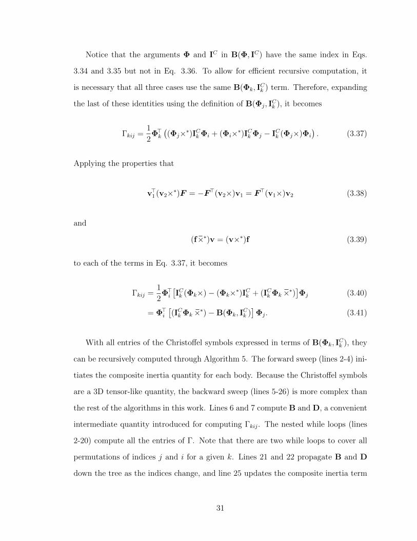
Notice that the arguments Φ and IC in B(Φ, IC) have the same index in Eqs.

3.34 and 3.35 but not in Eq. 3.36. To allow for efficient recursive computation, it

is necessary that all three cases use the same B(Φk, ICk ) term. Therefore, expanding

the last of these identities using the definition of B(Φj, ICk ), it becomes

Γkij =1

2Φ>k((Φj×∗)ICk Φi + (Φi×∗)ICk Φj − ICk (Φj×)Φi

). (3.37)

Applying the properties that

v>1 (v2×∗)F = −F>(v2×)v1 = F>(v1×)v2 (3.38)

and

(f×∗)v = (v×∗)f (3.39)

to each of the terms in Eq. 3.37, it becomes

Γkij =1

2Φ>i[ICk (Φk×)− (Φk×∗)ICk + (ICk Φk×∗)

]Φj (3.40)

= Φ>i[(ICk Φk×∗)−B(Φk, I

Ck )]Φj. (3.41)

With all entries of the Christoffel symbols expressed in terms of B(Φk, ICk ), they

can be recursively computed through Algorithm 5. The forward sweep (lines 2-4) ini-

tiates the composite inertia quantity for each body. Because the Christoffel symbols

are a 3D tensor-like quantity, the backward sweep (lines 5-26) is more complex than

the rest of the algorithms in this work. Lines 6 and 7 compute B and D, a convenient

intermediate quantity introduced for computing Γkij. The nested while loops (lines

2-20) compute all the entries of Γ. Note that there are two while loops to cover all

permutations of indices j and i for a given k. Lines 21 and 22 propagate B and D

down the tree as the indices change, and line 25 updates the composite inertia term

31

and velocity product factorizations as the algorithm sweeps towards the root of the

tree. Because each of the nested while loops has a computational cost proportional

to its depth, the overall efficiency of the algorithm is O(Nd2)

Algorithm 5 Christoffel Symbols Algorithm

Require: q,model1: v0 = 02: for i = 1 to N do3: ICi = Ii4: end for5: for k = N to 1 do6: B = 1

2[(Φk×∗)ICk + (ICk Φk)×∗ − ICk (Φk×)]

7: D = (ICk Φk×∗)−B8: j = k9: while j > 0 do10: F1 = B Φj

11: F2 = B>Φj

12: F3 = D Φj

13: i = j14: while i > 0 do15: Γijk = Γikj = Φ>1F1

16: Γjik = Γjki = Φ>1F2

17: Γkij = Γkji = Φ>1F3

18: F1 = iX>p(i)F1; F2 = iX>p(i)F2; F3 = iX>p(i)F3;

19: i = p(i)20: end while21: B = jX>p(j) B jXp(j)

22: D = jX>p(j) D jXp(j)

23: j = p(j)24: end while25: ICp(k) = ICp(k) + kX>p(k) ICk

kXp(k)

26: end for27: return Γ

32

3.3 Results

Algorithms 4 and 5 were implemented in C/C++ using the Rigid-Body Dynamics

Library [11]. This publicly available library exploits the sparsity patterns in quan-

tities in the equations of motion, such as the spatial inertia tensor, to minimize

computational cost and runtime of dynamics operations. This section presents the

results that verified the correctness and performance of the algorithms developed in

this chapter.

3.3.1 Validation

Three methods compared Algorithms 4 and 5 against known algorithms, such as

the RNEA, to verify their accuracy.

Method 1 : From the canonical equations of motion in Eq. 2.12, it is clear that

when the gravity force is 0 and q = 0, the torque at each joint is equal to the product

of C(q, q) and q. Therefore, if Algorithm 4 is correct, for a system under those

conditions, the torque τ computed through the RNEA and the computed C satisfy

Cq− τ = 0.

Method 2 : After C is verified with Method 1, the computed H is verified to satisfy

H− (C + C>) = 0.

Method 3 : Because of Eq. 3.26, with a correct C, the Christoffel symbols are

verified if they satisfy∑

k Γijk(q) qk −Cij = 0.

The three methods were tested using serial kinematic chains of 5, 10, and 15

bodies. The errors for all methods in all three scenarios were negligible, which verifies

the correctness of Algorithms 4 and 5 (Table 3.1).

3.3.2 Performance

For serial kinematic chains, where the depth equals the number of bodies, the com-

putational cost for the Coriolis matrix scales as O(N2), while that for the Christoffel

33

TABLE 3.1

VALIDITY CHECKS FOR SERIAL KINEMATIC CHAINS OF 5, 10,

AND 15 BODIES (MAXIMUM ERROR)

N = 5 N = 10 N = 15

Method 1 : Cq− τ (RNEA) 5.7× 10−14 7.3× 10−12 2.9× 10−11

Method 2 : H− (C + C>) 3.6× 10−15 5.7× 10−14 2.3× 10−13

Method 3 :∑

k[Γ1,1,k, qk]−C1,1 1.1× 10−13 7.3× 10−12 1.0× 10−12

symbols grows as O(N3) (Fig. 3.2). Note that these trends refer to the behavior

when the number of bodies is large because when N is low, the computational cost is

dominated by computations that do not scale with N , such as BC . For a branching

mechanism where d < N , the expected behavior is for the computational cost to

grow more slowly than in the serial case where d = N because O(Nd) < O(N2) and

O(Nd2) < O(N3). This behavior was confirmed by testing both algorithms on a

branching mechanism with a branching factor of 2. In this case, the time to com-

pute the Coriolis matrix grew roughly as O(N) and that of the Christoffel symbols

empirically scaled as O(N1.25) (Fig. 3.3). This branching effect is present in com-

mon robotic systems such as quadrupeds and bipeds. In particular, quadrupeds have

a higher branching factor than bipeds, so, as expected, the computational cost for

the Coriolis matrix and Christoffel symbols is higher in bipeds than in quadrupeds

(Fig. 3.4).

In terms of absolute time, Algorithms 4 and 5 proved to be fast enough for online

control loops that run thousands of times per second. For rigid-body systems of 20

DoFs, the algorithms take approximately 20 µs to compute the Coriolis matrix and up

34

Figure 3.2. Performance for serial kinematic chains.

Figure 3.3. Performance for branching mechanism (branching factor of 2).

35

Figure 3.4. Computation cost for bipeds and quadrupeds.

to 120 µs to calculate the Christoffel symbols (Table 3.2). The longer computation

times for the Christoffel symbols are associated with trees that have little to no

branching. In contrast, for kinematic trees with higher branching factors, all Γijk can

be computed in as little as 33 µs.

These results are particularly promising for the Christoffel symbols algorithm.

Commonly, the first step to symbolically compute Γijk is to calculate the mass matrix

symbolically with an algorithm such as CRBA or RNEA. Then it is necessary to do a

large number of partial derivatives of H to find the Christoffel symbols. This process

becomes prohibitively complex for systems with more than just a few bodies. To

show the capability of Algorithm 5, it was implemented using symbolic variables in

MATLAB. The algorithm calculates Γijk in a time comparable to that of the symbolic

implementation of the CRBA, which is only the first step of the alternative approach

to get Γijk (Table 3.3). This performance is even more remarkable when considering

the results of Table 3.2. In the time it takes to solve for H symbolically, Algorithm

36

TABLE 3.2

COMPUTATION TIME OF CORIOLIS MATRIX AND CHRISTOFFEL

SYMBOLS FOR COMMON RIGID-BODY SYSTEMS.

C(µs) Γijk(µs)

Serial Chain (20 DoF) 18 122

Branching Mechanism (20 DoF) 10 33

Biped (20 DoF) 18 122

Quadruped (19 DoF) 10 37

5 can numerically compute Γijk more than 3,000 times.

3.4 Conclusion

This section developed computationally efficient algorithms to numerically solve

for the Coriolis matrix and its associated Christoffel symbols. The algorithms exploit

the bi-linearity in v and I of a suitable body-level factorization, B(v, I), of velocity

product terms when computing the system-level Coriolis terms. In Algorithm 4, the

newfound expressions for each entry in the Coriolis matrix are computed recursively

in terms of composite quantities ICi and BCi . Taking the derivative for the expression

of Cij with respect to qk allowed new expressions for the Christoffel symbols in terms

of B(vi, Ii) that are computed recursively in Algorithm 5. Both algorithms proved

to be fast and of the lowest order possible. Their complexity grew as O(Nd) and

O(Nd2), respectively, while their computation time was on the order of µs. For a

20-DoF biped, it took the algorithms only 17 µs to compute C and 123 µs for Γ.

The effects of branching played a substantial role in decreasing runtime, particularly

37

TABLE 3.3

RUNTIME OF ALGORITHMS USING SYMBOLIC VARIABLES FOR

SERIAL CHAINS WITH 5,10, AND 15 BODIES.

N = 5 (s) N = 10 (s) N = 15 (s)

H 0.06 0.18 0.36

Γijk 0.25 1.11 2.13

for the Christoffel symbols algorithm. For a 19-DoF quadruped, the computational

time for Algorithm 5 reduced to 38 µs. Given the efficiency, scalability, and speed

of these algorithms, they are viable for implementation in real-time control loops as

well as other dynamics applications.

38

CHAPTER 4

MODIFIED ARTICULATED-BODY ALGORITHM

4.1 Introduction

This chapter presents the derivation of a modified Articulated-Body Algorithm

(MABA) that accurately accounts for the inertia of motor rotors. The chapter first

introduces the necessary formalisms for the derivation: the Gauss Principle of Least

Constraint and the model used to describe geared electric motors. The chapter shows

that by reformulating the dynamics of the system as an optimization problem through

the Gauss Principle of Least Constraint, it is possible to adjust the quantities of the

ABA to account for rotor inertias from first principles. The chapter discusses the

validity of the proposed algorithm by comparing its results with those of the ABA

and other common methods to approximate the inertial effects of actuators. The

chapter also discusses the performance of the modified ABA in terms of complexity

and runtime.

4.2 Mathematical Formalisms and Modeling Conventions

4.2.1 Gauss Principle of Least Constraint

The Gauss Principle of Least Constraint is a formulation of mechanics used to

solve for the admissible accelerations of constrained mechanical systems [31]. The

principle is described in terms of a least-squares optimization problem. In particular,

it states that the accelerations of a system of rigid bodies deviate from the uncon-

strained accelerations in a least-squares sense. Mathematically, the principle specifies

39

that [6]

argmin{ai}

∑i

(ai − auci )>Ii(ai − auci )

subject to {ai} satisfy constraints,

(4.1)

where auci is the unconstrained acceleration of body i. While this principle originally

considered only massive point particles, it is also valid for rigid-body systems that

are geometrically constrained by considering the inertia tensor as opposed to just the

mass of each body.

An unconstrained system (Figure 4.1b) is one in which the bodies are not geo-

metrically constrained so that the dynamics of each body are entirely independent of

the dynamics of the rest of the bodies in the system. Then, the unconstrained accel-

erations are the accelerations caused by external forces acting on individual particles,

ignoring all forces from constrained interactions between bodies.

A constrained system (Figure 4.1a) is one in which bodies are geometrically con-

strained so that the dynamics of each body are coupled with those of other bodies.

Because bodies are constrained, the overall dynamics of the system limit the possible

values for each ai. The true accelerations are calculated by solving the optimization

problem in the Gauss Principle of Least Constraint.

Overall, the Gauss Principle of Least Constraint provides an intuitive mathemat-

ical framework to solve the forward dynamics problem for complex systems that are

common in robotics applications.

4.2.2 Joint Modeling

Previous attempts to use the Gauss Principle of Least Constraint to model kine-

matic chains have mostly ignored the inertial effects of rotors and gears [29]. It is

necessary to include these elements in the model of each joint to account for their

inertial effects. This work considers joints to be as shown in Figure 4.2. The dis-

40

(a) Constrained System(b) Unconstrained System

Figure 4.1. Visual comparison between constrained and unconstrainedsystems.

assembled joint in this figure is composed of body p(i), rotor Ri, gearbox Gi, and

body i so that these four elements form a kinematic loop. Notice that the model

for the gearing of the joint is one body linked to the rotor, so all internal forces and

friction associated with gear dynamics are ignored. Similarly, the model assumes

that the gearbox is massless and without any inertia. For most robotics systems, this

assumption is valid because motor rotors are often several times heavier than their

gears.

A particularly important consequence of the joint model used in this work is that

the term describing the free modes of motion of rotor Ri must be equal to the term

describing the free modes of motion of body i because the rotor is rotating along

the same axis as the body. While the proposed joint model does not account for all

interactions inside the joint, it provides a more accurate representation than what

dynamics algorithms in the literature commonly use. Furthermore, the mathematical

methods presented in this chapter can easily expand to include other terms such as

gearing inertia or internal friction to obtain an even more accurate account of joint

inertial effects.

41

Figure 4.2. Dissasembled joint between body p(i) and body i

4.3 Algorithm Derivation

The general strategy to derive an ABA that accounts for rotor inertias from

first principles is as follows. First, determine expressions for the constrained and

unconstrained accelerations of body i, as well as rotor Ri. Then solve the optimization

problem for the Gauss Principle of Least Constraint for a single body subject to the

appropriate constraints. Then find expressions for the articulated inertia and bias

forces based on the solution of the optimization problem and use the new expression

within the structure of the ABA to solve the forward dynamics problem. Similar to

Chapter 3, the derivation in this chapter uses coordinate-free expressions, but the

algorithm shows the appropriate transformation matrices.

4.3.1 Identification of Optimization Problem

Consider the unconstrained case for the joint in Figure 4.2. The only two forces

present in the unconstrained system are a torque and its equal and opposite reaction.

42

Then, according to the ABA definition of force in terms of articulated quantities from

Eq. 2.19, the unconstrained acceleration of body i is

auci = (IAi )−1(Φiτ i − pAi ), (4.2)

where pAi is an associated bias force.

Similarly, the rotor feels the same forces, but its unconstrained acceleration is

expressed a bit differently. In particular, because the torque felt by body i is the

output torque of the motor multiplied by the gear ratio of the gearbox, ni, the torque

felt by the motor is τ i divided by ni. Furthermore, because the inertia the rotor feels

is only its own, the unconstrained acceleration of Ri is given by

aucRi= I−1Ri

(Φiτ ini− pRi

), (4.3)

where pRi= vRi

×∗ IRivRi

and vRi= vp(i) + Φiqini is the spatial velocity of the

rotor.

Now consider the constrained case. When the joint is assembled, the admissible

accelerations of each joint are limited by the accelerations of the rest of the kinematic

tree. Therefore, the constrained acceleration of body i is simply given by Eq. 2.16

as ai = ap(i) + Φiqi + (vi×)Φiqi. A similar expression applies for the constrained

acceleration of the rotor. Notably, the changes to Eq. 2.16 are that the joint velocity

and acceleration of Ri are equal to the joint velocity and acceleration of body i

multiplied by the gear ratio ni because of the effects of the gearbox. Then, the

equation for the constrained acceleration of Ri becomes

aRi= ap(i) + Φiqini + (vRi

×)Φiqini. (4.4)

From the Gauss Principle of Least Constraint, the acceleration of each body must

43

minimally deviate from its unconstrained acceleration at any given joint. Therefore,

an appropriate reformulation of Eq. 4.1 that accounts for rotor inertias is given by

argminqi

(ai − auci )>IAi (ai − auci ) + (aRi− aucRi

)>IRi(aRi− aucRi

)

where ai = ap(i) + Φiqi + (vi×)Φiqi, and

aRi= ap(i) + Φiqini + (vRi

×)Φiqini.

(4.5)

4.3.2 Solving the Optimization Problem

Expanding the objective function of Eq. 4.5 it yields

z = a>i IAi ai− 2a>i I

Ai auci + (auci )>IAi auci + a>Ri

IRiaRi− 2a>Ri

IRiaucRi

+ (aucRi)>IRi

aucRi. (4.6)

To solve the optimization problem presented by the Gauss Principle of Least Con-

straint, this expression must be differentiated with respect to q, so any terms that

do not depend on q will become 0 after differentiation. From the definitions of un-

constrained accelerations for body and rotors in Eqs. 4.2 and 4.3, these terms do

not depend on q. Any terms in the objective function that depend solely on uncon-

strained accelerations will become irrelevant for the solution of Eq. 4.5. Thus, the

relevant terms of the objective function are

z1 = a>i IAi ai − 2a>i I

Ai auci , (4.7)

and

z2 = a>RiIRi

aRi− 2a>Ri

IRiaucRi

. (4.8)

Consider first the terms of body i, z1. Substituting the constraints into the

44

relevant terms of the objective function, the expression becomes

z1 = (ap(i) + Φiqi + (vi×)Φiqi)>IAi (ap(i) + Φiqi + (vi×)Φiqi)

− 2(ap(i) + Φiqi + (vi×)Φiqi)>IAi auci .

(4.9)

Further removing terms that are not dependent on q, the expression simplifies to

z1 = q>i Φ>i IAi Φiqi + 2q>i Φ

>i IAi (ap(i) + (vi×)Φiqi)− 2q>i Φ

>i IAi auci . (4.10)

Taking the gradient of Eq. 4.10 with respect to qi,

∂z1∂qi

= 2Φ>i IAi Φiqi + 2Φ>i I

Ai (ap(i) + (vi×)Φiqi)− 2Φ>i I

Ai auci . (4.11)

Now consider the terms of rotor Ri, z2. Again, the expression simplifies by dis-

carding the terms that do not depend on q. The expression further simplifies by

defining the quantity ΦRi= Φini so that the expression for z2 becomes

z2 = q>i Φ>Ri

IRiΦRi

qi + 2q>i Φ>Ri

IRi(ap(i) + (vRi

×)ΦRiqi)− 2q>i Φ

>Ri

IRiaucRi

. (4.12)

Taking the gradient,

∂z2∂qi

= 2Φ>RiIRi

ΦRiqi + 2Φ>Ri

IRi(ap(i) + (vRi

×)ΦRiqi)− 2Φ>Ri

IRiaucRi

. (4.13)

Now, by adding Eqs. 4.11 and 4.13 and equating to 0, the full equation to find q

is

0 =∂z

∂qi=∂z1∂qi

+∂z2∂qi

(4.14)

45

so that

0 = 2Φ>i IAi Φiqi+2Φ>i I

Ai (ap(i) + (vi×)Φiqi)− 2Φ>i I

Ai auci

+ 2Φ>RiIRi

ΦRiqi + 2Φ>Ri

IRi(ap(i) + (vRi

×)ΦRiqi)− 2Φ>Ri

IRiaucRi

.

(4.15)

For simplicity of notation, before solving for the optimal q, the following new

quantities are defined.

Di = Φ>i IAi Φi + Φ>Ri

IRiΦRi

, (4.16)

ξi = (vi×)Φiqi, (4.17)

and

ξRi= (vRi

×)ΦRiqi. (4.18)

Solving Eq. 4.15 yields that the optimal qi is expressed in terms of the new

quantities as

qi = −D−1i Φ>i IAi (ap(i) + ξi − auci )−D−1i Φ>Ri

IRi(ap(i) + ξRi

− aucRi). (4.19)

4.3.3 Finding Recursive Relations

The qi obtained through the Gauss Principle of Least Constraint in Eq. 4.19 has

the remarkable property of being independent of the dynamics at other joints. If

the articulated-body inertia and bias force of each body are known, qi and ai can

be computed recursively. This subsection is dedicated to finding expressions for the

articulated-body inertia and bias force given the new definition of qi.

Consider a test force on body p(i) (Figure 4.3) so that

fp(i) = Ip(i)ap(i) + pp(i) + IAi ai + pAi + IRiaRi

+ pRi. (4.20)

46

This force is also equal to the articulated terms based on Featherstone’s definition in

Eq. 2.19, so the equations becomes

IAp(i)ap(i) + pAp(i) = Ip(i)ap(i) + pp(i) + IAi ai + pAi + IRiaRi

+ pRi. (4.21)

Figure 4.3. Force acting on body p(i).

Expanding the terms IAi ai and IRiaRi

in terms of q,

IAi ai = IAi (ap(i) −Φiqi + ξi), (4.22)

IRiaRi

= IRi(ap(i) −ΦRi

qi + ξRi). (4.23)

By substituting Eqs. 4.19, 4.22 and 4.23 into Eq. 4.21 the updated definitions of

47

articulated inertia and the articulated bias force become

IAp(i) = Ip(i) + IAi + IRi− IAi ΦiD

−1i Φ>i I

Ai − IRi

ΦRiD−1i Φ>Ri

IRi(4.24)

and

pAp(i) = pp(i) + pAi + pRi+ IAi ξi + IRi

ξRi+ IAi ΦiD

−1i Φ>i I

Ai auci − IAi ΦiD

−1i Φ>i I

Ai ξi

+ IRiΦRi

D−1i Φ>RiIRi

aucRi− IRi

ΦRiD−1i Φ>Ri

IRiξRi

.

(4.25)

4.3.4 Modified Articulated-Body Algorithm

Using the updated IAp(i) and pAp(i), the modified ABA is shown in Algorithm 6. The

structure is almost identical to that of the regular ABA. There is one sweep forward

to initialize articulated terms and propagate velocities (lines 1-6), a backward pass

to update the articulated terms (lines 8-20), and a final forward sweep to compute

the joint rates and accelerations of each body (lines 21-24).

4.4 Results

Algorithm 6 was implemented in MATLAB using the Spatial v2 package for rigid-

body dynamics developed by Roy Featherstone [9]. This section presents the validity

and performance checks that verify the correctness and efficiency of the algorithm.

Unless otherwise noted, all tests performed in this chapter consider mechanisms

where all bodies are thin-walled cylinders of mass of 1 kg and length 1 m with q = 0

and gravity equal to 0. All rotors have a mass of 0.5 kg and a gear ratio of 5.

Furthermore, the torque and joint position at each joint are set equal to the number

of the joint in N·m and radians, respectively. For example, τ 2 = 2 N·m, and q14 = 14

rad.

48

Algorithm 6 Articulated-Body Algorithm

Require: q,model1: for i = 1 to N do2: IAi = Ii3: ΦRi

= Φini4: pAi = vi ×∗ Iivi5: pRi

= vRi×∗ IRi

vRi

6: vi = iXp(i)vp(i) + Φiqi7: vRi

= RiXp(i)vp(i) + ΦRiqi

8: ξi = (vi×)Φiqi9: ξRi

= (vRi×)ΦRi

qi10: end for11: for i = N to 1 do12: auci = (IAi )−1(Φiτ i − pAi )13: aucRi

= I−1Ri(Φi

τ i

ni− pRi

)

14: Di = Φ>i IAi Φi + Φ>Ri

IRiΦRi

15: if p(i) 6= 0 then16: IAp(i) = Ip(i) + iX>p(i)[I

Ai + IRi

− IAi ΦiD−1i Φ>i I

Ai − IRi

ΦRiD−1i Φ>Ri

IRi]iXp(i)

17: pAp(i) = pp(i) + iX>p(i)[pAi + pRi

+ IAi ξi + IRiξRi

+ IAi ΦiD−1i Φ>i I

Ai (auci − ξi) +

IRiΦRi

D−1i Φ>RiIRi

(aucRi− ξRi

)]iXp(i)

18: end if19: end for20: for i = 1 to N do21: qi = −D−1i Φ>i [IAi (iXp(i)ap(i) + ξi − auci ) + niIRi

(iXp(i)ap(i) + ξRi− aucRi

)]22: ai = iXp(i)ap(i) + Φiqi + (vi×)Φiqi23: end for24: return q, a

49

TABLE 4.1

CONSISTENCY CHECK FOR A SERIAL KINEMATIC CHAINS OF 5,

10, AND 15 BODIES (MAXIMUM ERROR)

N = 5 (N·m) N = 10 (N·m) N = 15 (N·m)

τ − τRNEA 4.3× 10−14 4.3× 10−13 2.4× 10−13

4.4.1 Validation

Method 1: Self-consistency. If the algorithm is mathematically consistent, the

inverse and forward dynamics must truly be the inverse of each other. To verify

this is the case, the q computed via Algorithm 6 became the input for the RNEA

that computes the torque at each joint. This procedure checked the results for serial

kinematic chains of 5,10 and 15 bodies. The torques from the RNEA in all of these

cases match the initial input torques for the modified ABA (Table 4.1); therefore,

the algorithm is consistent.

Method 2: Comparison to usual approximation methods. In the industrial set-

ting where actuators tend to have large gear ratios, the inertial effects of rotors are

approximating by modifying the mass matrix in the CRBA. The motor inertia term

Φ>i IRiΦin

2i adds to the diagonal entries of H. Then according to the canonical equa-

tions of motion, q is computed with a new H as

q = H−1(τ −Cq− g). (4.26)

When the actuators are inertialess, the modified CRBA (MCRBA), the modified

ABA in Algorithm 6 and the regular ABA should produce the same results. Similarly,

50

TABLE 4.2

MAXIMUM DIFFERENCE IN q FOR SERIAL CHAINS WITH 5, 10,

AND 15 BODIES WITH INERTIALESS ACTUATORS.

N = 5 (rad·s−2) N = 10 (rad·s−2) N = 15 (rad·s−2)

MABA and ABA 8.4× 10−15 2.9× 10−14 1.9× 10−13

MABA and MCRBA 1.5× 10−14 6.1× 10−14 2.2× 10−13

MCRBA and ABA 6.2× 10−15 6.7× 10−14 2.1× 10−13

when the rotors’ inertia is significant, MABA’s results must be closer to those of

MCRBA’s approximation than the results of the regular ABA. Differences between

MABA and MCRBA results are inevitable because Algorithm 6 is exact, whereas the

other is an approximation.

Consider serial kinematic chains of 5, 10 and 15 bodies. As expected, for the case

when IRi= 0, all three algorithms produce the same results without variation (Table

4.2). In contrast, when the rotors’ inertia is significant, the ABA produces results

that are vastly different from those of the other two algorithms, but the results from

MABA and MCRBA are equal to multiple decimal places. This is the case for serial

chains as well as branched mechanisms (Tables 4.3 and 4.4), which speaks to the

correctness of Algorithm 6.

The close agreement between MABA and MCRBA in these tests is contingent

upon q = 0. When q 6= 0, there are Coriolis terms from the rotor that are completely

ignored by the CRBA. If q is not close to 0, the Coriolis terms become significant

so that MCRBA is no longer valid. Consider serial kinematic chains of 5, 10, and

15 bodies as in previous cases, but with q = π2

rad·s−1 for all joints. In this case,

51

TABLE 4.3

MAXIMUM DIFFERENCE IN q FOR SERIAL CHAINS WITH 5, 10,

AND 15 BODIES.

N = 5 (rad·s−2) N = 10 (rad·s−2) N = 15 (rad·s−2)

MABA and ABA 23.12 39.14 57.72

MABA and MCRBA 0.026 0.037 0.062

MCRBA and ABA 23.15 39.18 57.79

the difference in q between MABA and CRABA can be as large as hundreds of

rad·s−2 (Table 4.5). When the discrepancies are this large, MABA provides the most

accurate results. Because MABA accounts for rotor inertia from first principles, the

Coriolis terms are implicitly accounted for in Algorithm 6, which makes it much more

accurate than MCRBA under these circumstances.

4.4.2 Performance

The benchmarking performance of Algorithm 6 included serial kinematic chains

and branching mechanisms with a branching factor of 2. As expected, the algorithm’s

complexity grew as O(N), matching the performance of the regular ABA (Figure 4.4).

Furthermore, branching had no effects on the computational time of the algorithm

(Figure 4.5). Because the algorithm has no loop that runs through the ancestors of

each body within the middle backward pass, the depth of each branch has no effect

on complexity.

In terms of runtime, Algorithm 6 performed similarly to the regular ABA (Table

4.6). The difference between the runtime of both algorithms is less than a millisecond,

52

Figure 4.4. Computation time for serial kinematic chains.

Figure 4.5. Computation time for branching mechanism (branching factorof 2).

53

TABLE 4.4

MAXIMUM DIFFERENCE IN q FOR BRANCHING MECHANISM

WITH 5, 10, AND 15 BODIES (BRANCHING FACTOR OF 2).

N = 5 (rad·s−2) N = 10 (rad·s−2) N = 15 (rad·s−2)

MABA and ABA 28.16 79.64 179.38

MABA and MCRBA 0.037 0.070 0.11

MCRBA and ABA 28.19 79.69 179.47

and it is because the expressions for the articulated terms in Algorithm 6 are much

more computationally expensive than those in the ABA. Still, Algorithm 6 proved

to be fast. It can solve the forward dynamics problem a thousand times per second.

Note that the times in Table 4.6 come from implementation in MATLAB, so times

can improve significantly if the algorithm runs using a compiled language such as

C++.

4.5 Conclusion

The work presented in this chapter shows that considering rigid-body dynamics

as an optimization problem through the Gauss Principle of Least Constraint allows

for more accurate dynamics algorithms. In particular, the chapter showed how by

adding rotor inertia terms and solving the optimization problem, it is possible to

find a Modified Articulated-Body Algorithm that accounts for rotor inertias from

first principles. The chapter also showed how the proposed algorithm compares to

a common approximation of actuators’ inertial effects and how its complexity and

runtime match those of the regular Articulated-Body Algorithm.

54

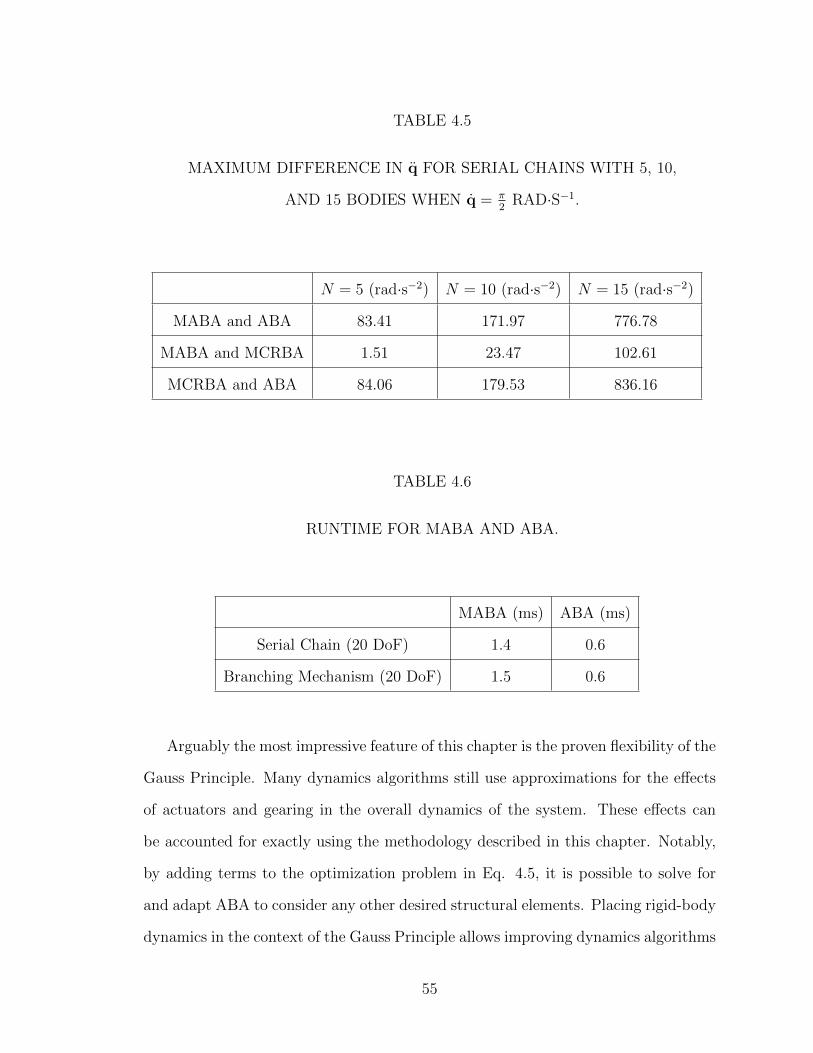
TABLE 4.5

MAXIMUM DIFFERENCE IN q FOR SERIAL CHAINS WITH 5, 10,

AND 15 BODIES WHEN q = π2

RAD·S−1.

N = 5 (rad·s−2) N = 10 (rad·s−2) N = 15 (rad·s−2)

MABA and ABA 83.41 171.97 776.78

MABA and MCRBA 1.51 23.47 102.61

MCRBA and ABA 84.06 179.53 836.16

TABLE 4.6

RUNTIME FOR MABA AND ABA.

MABA (ms) ABA (ms)

Serial Chain (20 DoF) 1.4 0.6

Branching Mechanism (20 DoF) 1.5 0.6

Arguably the most impressive feature of this chapter is the proven flexibility of the

Gauss Principle. Many dynamics algorithms still use approximations for the effects

of actuators and gearing in the overall dynamics of the system. These effects can

be accounted for exactly using the methodology described in this chapter. Notably,

by adding terms to the optimization problem in Eq. 4.5, it is possible to solve for

and adapt ABA to consider any other desired structural elements. Placing rigid-body

dynamics in the context of the Gauss Principle allows improving dynamics algorithms

55

further to be more accurate and flexible in accounting for the different characteristics

of modern-day actuators.

56

CHAPTER 5

CONCLUSIONS

5.1 Summary and Conclusions

The results presented in this work showcase that algorithms to compute the Cori-

olis matrix, its Christoffel symbols, and the inertial effects of motor rotors are viable

for real-time implementation in model-based control applications. Three recursive al-

gorithms, the Recursive Newton-Euler Algorithm, the Articulated-Body Algorithm,

and the Composite Rigid-Body Algorithm, were reviewed. These algorithms are

widely used for many robotics applications and provide the framework needed to

develop new algorithms that expand the capacity to compute other dynamic terms

numerically.

Then, using a suitable body-level factorization of the velocity product terms, it

was possible to develop a recursive algorithm to compute each entry in the Coriolis

matrix in terms of composite quantities in CRBA style. Then, taking the deriva-

tives of the expressions in the Coriolis matrix algorithm leads to an expression for

the Christoffel symbols in terms of body-level factorization terms that can be com-

puted recursively in an algorithm. These two algorithms are of the lowest possible

complexity, O(Nd) and O(Nd2), respectively, and their runtimes are on the order

of a few tens of µs for systems with 20 DoF. The performance of both algorithms

provides a scalable, efficient, and fast alternative to other algorithms and approxi-

mation methods. These results are particularly promising for the Christoffel symbols

algorithm because it is thousands of times faster than other alternatives available in

the literature involving symbolic partial derivatives.

57

This thesis also showed how the Gauss Principle of Least Constraint makes it

possible to derive an algorithm that accounts for rotor inertias from first principles

by adding terms to the objective function of the optimization problem as well as rel-

evant constraints. This algorithm uses the same structure as the Articulated-Body

Algorithm, but it has expressions for the articulated terms that include the inertial

effects of actuators. This algorithm is of equal complexity and similar runtime as

the original Articulated-Body Algorithm, which makes it viable for implementation

in real-time controllers or rapid simulation for learning-based control design strate-

gies. This new algorithm offers a much more accurate alternative to the regular

Articulated-Body Algorithm when the inertial effects of the rotors are significant.

In conclusion, this thesis used numerical methods to derive new rigid-body dy-

namics algorithms that are feasible for implementation in model-based controllers

that require dynamics calculations as part of their control scheme. The presented

algorithms proved to meet or exceed the performance of other currently available

algorithms in the literature. Because of their scalability, accuracy, and speed, the

algorithms developed in this work are valid candidates for real-time implementation

in applications of sensorless contact detection, passivity-based control, and adaptive

control.

5.2 Future Work

All the results presented in this work were obtained through computer simulations

of simple rigid-body systems. While these results successfully prove, in theory, the

accuracy and viability of the algorithms presented in this thesis, further empirical

evidence is needed for establishing the true capabilities of these algorithms. First,

implementing the Coriolis matrix algorithm in the real-time control of a robot that

uses sensorless contact detection, such as MIT’s Cheetah robot, will provide empir-

ical data for how fast and accurate the algorithm is under practical circumstances.

58

Similarly, implementing the Christoffel symbols algorithm in geometric controllers

that use approximations for the Christoffel symbols will allow measuring how this

new algorithm might improve the performance of certain physical robots.

Another research avenue regarding the Modified Articulated-Body Algorithm is to

expand it further to include other inertial effects. Adding gears and internal friction

might significantly improve the accuracy of the algorithms, particularly in physical

systems where the gearing system has comparable mass to the motor. Furthermore,

the joint model used to develop the Modified Articulated-Body Algorithm assumes

that the free modes of motion of the rotor and the body are the same. This assump-

tion limits the applicability of the algorithm to systems with basic revolute joints.

Forgoing this assumption allows making the algorithm fully general and applicable

to any physical system. Then, a rederivation of the algorithm with more complicated

expressions for the articulated terms is required.

Further work for the Modified Articulated-Body Algorithm involves physical sys-

tems. The implementation of this algorithm with a physical robot with significant in-

ertial effects from the actuators will measure how accurate this algorithm is compared

to the regular Articulated-Body Algorithm and the Modified Composite Rigid-Body

Algorithm approximation. Obtaining data points from different physical systems

will allow developing a metric to determine when different approximations and algo-

rithms are no longer valid due to the inertial effects from actuators. Further research

involving the characterization of inertial effects of different structural components

provides opportunities to fine tune the Modified Articulated-Body Algorithm and

further improve its accuracy.

59

BIBLIOGRAPHY

1. Springer Handbook of Robotics. Springer handbooks. Springer InternationalPublishing : Imprint: Springer, Cham, 2nd edition.. edition, 2016. ISBN9783319325521.

2. G. Bledt, P. Wensing, S. Ingersoll, and S. Kim. Contact model fusion for event-based locomotion in unstructured terrains. pages 4399–4406, May 2018. doi:10.1109/ICRA.2018.8460904.

3. J. Bobrow, F. Park, and A. Sideris. Recent Advances on the Algorithmic Op-timization of Robot Motion, pages 21–41. Springer Berlin Heidelberg, Berlin,Heidelberg, 2006. ISBN 978-3-540-36119-0. doi: 10.1007/978-3-540-36119-0 2.URL https://doi.org/10.1007/978-3-540-36119-0_2.

4. A. Carvalho and A. Suleman. Simulation of rigid-body impact using thearticulated-body algorithm. Robotica, 29(5):649–656, 2011. ISSN 02635747. URLhttp://search.proquest.com/docview/899301478/.

5. A. De Luca and L. Ferrajoli. A modified newton-euler method for dynamiccomputations in robot fault detection and control. In 2009 IEEE InternationalConference on Robotics and Automation, pages 3359–3364. IEEE, 2009. ISBN9781424427888.

6. Y. Fan, R. Kalaba, H. Natsuyama, and F. Udwadia. Reflections on the gaussprinciple of least constraint. Journal of Optimization Theory and Applications,127(3):475–484, 2005. ISSN 0022-3239.

7. R. Featherstone. The calculation of robot dynamics using articulated-body in-ertias. The International Journal of Robotics Research, 2(1):13–30, 1983. ISSN0278-3649.

8. R. Featherstone. Rigid body dynamics algorithms. Springer, New York, 2008.ISBN 9780387743158.

9. R. Featherstone, Feb 2015. URL http://royfeatherstone.org/spatial/v2/

index.html#ID.

10. R. Featherstone and D. Orin. Robot dynamics: equations and algorithms. InProceedings 2000 ICRA. Millennium Conference. IEEE International Conferenceon Robotics and Automation. Symposia Proceedings (Cat. No.00CH37065), vol-ume 1, pages 826–834 vol.1. IEEE, 2000. ISBN 0780358864.

60

11. M. L. Felis. Rbdl: an efficient rigid-body dynamics library using recursive algo-rithms. Autonomous Robots, pages 1–17, 2016. ISSN 1573-7527. doi: 10.1007/s10514-016-9574-0. URL http://dx.doi.org/10.1007/s10514-016-9574-0.

12. J. M. Hollerbach. A recursive lagrangian formulation of maniputator dynamicsand a comparative study of dynamics formulation complexity. IEEE Transactionson Systems, Man, and Cybernetics, 10(11):730–736, 1980. ISSN 0018-9472.

13. A. Jain and G. Rodriguez. Recursive linearization of manipulator dynamics mod-els. In 1990 IEEE International Conference on Systems, Man, and CyberneticsConference Proceedings, pages 475–480. IEEE, 1990. ISBN 0879425970.

14. A. Jain and G. Rodriguez. Linearization of manipulator dynamics using spatialoperators. IEEE Transactions on Systems, Man, and Cybernetics, 23(1):239–248,1993. ISSN 0018-9472.

15. O. Khatib. A unified approach for motion and force control of robot manipulators:The operational space formulation. IEEE Journal on Robotics and Automation,3(1):43–53, 1987. ISSN 0882-4967.

16. J. Luh, M. Walker, and R. Paul. On-line computational scheme for mechanicalmanipulators. Journal of Dynamic Systems, Measurement and Control, Trans-actions of the ASME, 102(2):69–76, 1980. ISSN 00220434.

17. J. Murray and D. Johnson. The linearized dynamic robot model: efficient com-putation and practical applications. In Proceedings of the 28th IEEE Conferenceon Decision and Control, pages 1659–1664 vol.2. IEEE, 1989.

18. J. Murray and C. Neuman. Organizing customized robot dynamics algorithmsfor efficient numerical evaluation. IEEE Transactions on Systems, Man, andCybernetics, 18(1):115–125, 1988. ISSN 0018-9472.

19. A. Mller and Z. Terze. Geometric methods and formulations in computationalmultibody system dynamics. Acta Mechanica, 227(12):3327–3350, 2016. ISSN00015970. URL http://search.proquest.com/docview/1846648706/.

20. G. Niemeyer and J.-J. E. Slotine. Performance in adaptive manipulator control.The International Journal of Robotics Research, 10(2):149–161, 1991. ISSN 0278-3649.

21. E. Otten. Inverse and forward dynamics: models of multibody systems. Philo-sophical Transactions of the Royal Society B: Biological Sciences, 358(1437):1493–1500, 2003. ISSN 0962-8436.

22. L. Righetti, J. Buchli, M. Mistry, M. Kalakrishnan, and S. Schaal. Optimaldistribution of contact forces with inverse-dynamics control. The InternationalJournal of Robotics Research, 32(3):280–298, 2013. ISSN 0278-3649.

61

23. C. Semini, N. Tsagarakis, E. Guglielmino, M. Focchi, F. Cannella, and D. Cald-well. Design of hyq -a hydraulically and electrically actuated quadruped robot.Proceedings of the Institution of Mechanical Engineers. Part I: Journal of Systemsand Control Engineering, 225:831–849, 08 2011. doi: 10.1177/0959651811402275.

24. B. Siciliano, L. Sciavicco, L. Villani, and G. Oriolo. Robotics: Modelling, Planningand Control. 2009. ISBN 9781846286414. URL http://search.proquest.com/

docview/35584129/.

25. J.-J. E. Slotine and W. Li. On the adaptive control of robot manipulators. TheInternational Journal of Robotics Research, 6(3):49–59, 1987. ISSN 0278-3649.

26. G. A. Sohl and J. E. Bobrow. A recursive multibody dynamics and sensitivityalgorithm for branched kinematic chains. Journal of Dynamic Systems, Measure-ment, and Control, 123(3):391, 2001. ISSN 0022-0434.

27. W. Suleiman, E. Yoshida, J.-P. Laumond, and A. Monin. Optimizing humanoidmotions using recursive dynamics and lie groups. In 2008 3rd International Con-ference on Information and Communication Technologies: From Theory to Ap-plications, pages 1–6. IEEE, 2008. ISBN 9781424417513.

28. M. Takegaki and S. Arimoto. A new feedback method for dynamic control ofmanipulators. Journal of Dynamic Systems, Measurement and Control, Trans-actions of the ASME, 103(2):119–125, 1981. ISSN 00220434.

29. A. Vereshchagin. Computer simulation of the dynamics of complicated mecha-nisms of robot-manipulators. Eng Cybern, 12(6):65–70, 1974.

30. P. Wensing, R. Featherstone, and D. E. Orin. A reduced-order recursive algo-rithm for the computation of the operational-space inertia matrix. In 2012 IEEEInternational Conference on Robotics and Automation, pages 4911–4917. IEEE,2012. ISBN 9781467314039.

31. K. Yunt. Gauss’ principle and principle of least constraints for dissipative me-chanical systems. IFAC Proceedings Volumes, 45(2):842–847, 2012. ISSN 1474-6670.

62