rights / license: research collection in copyright - non ...47191/... · my phd thesis in his...
TRANSCRIPT

Research Collection
Doctoral Thesis
Control of Electric Polarisation by Magnetic Fields in Spin-SpiralMultiferroics
Author(s): Leo, Naëmi Riccarda
Publication Date: 2014
Permanent Link: https://doi.org/10.3929/ethz-a-010346799
Rights / License: In Copyright - Non-Commercial Use Permitted
This page was generated automatically upon download from the ETH Zurich Research Collection. For moreinformation please consult the Terms of use.
ETH Library

DISS. ETH NO. 22347
CONTROL OF ELECTRIC POLARISATIONBY MAGNETIC FIELDS IN
SPIN-SPIRAL MULTIFERROICS
A thesis submitted to attain the degree ofDOCTOR OF SCIENCES of ETH ZURICH
(Dr. sc. ETH Zurich)
presented by
NAËMI RICCARDA LEO
Dipl.-Phys., Universität Bonn
born on 17.05.1985,
citizen of Germany
accepted on the recommendation of
Prof. Dr. Manfred FiebigProf. Dr. Nicola SpaldinDr. Michel Kenzelmann
2014


Declaration of Originality
I hereby declare that the following submitted thesis is originalwork which I alone have authored and which is written in myown words.
Title: Control of electric polarisation by magneticfields in spin-spiral multiferroics
Author: Leo, Naëmi RiccardaSupervisor: Prof. Dr. Manfred Fiebig
With my signature I declare that I have been informed regard-ing normal academic citation rules. The conventions usual tothe discipline in question here have been respected.
Furthermore, I declare that I have truthfully documented allmethods, data, and operational procedures and not manipu-lated any data. All persons who have substantially supportedme in my work are identified in the acknowledgements.
The above work may be tested electronically for plagiarism.
Zürich, November 26, 2014
iii


Acknowledgements
First of all, I would like to thank Prof. Manfred Fiebig for the opportunity to domy PhD thesis in his group, both at University Bonn and at ETH Zürich. Apartfrom the interesting discussions, I especially appreciated the opportunity to attendscientific meetings, and to teach various courses. Furthermore, I thank both Prof.Nicola Spaldin and Dr. Michel Kenzelmann for being part of the examiner board.I especially thank Prof. Pierre Tolédano for tutoring me in the arts of Landautheory. Also I am grateful for the discussions with Prof. Roman Pisarev, Prof. PetraBecker-Bohatý, and Prof. Ladislav Bohatý about optical material properties.
I thank all former and present members of the Hikari and Ferroic group for thehelp both in and out of the labs, and the nice excursions. It was fun working withyou, and I do hope you will never run out of Schoko Bons ,.In particular I want to thank Martin Lilienblum and Carsten Becher, my brothers inarms. I think we were a good team, and thank you so much for all the scientificand non-scientific support, especially during the last three years. Hopefully youwill never tire of tasty Swiss desserts.I also would like to thank Dennis Meier for interesting project proposals, and TimHoffmann, Sebastian Manz, Morgan Trassin, Matthias Ackermann, and AndreaScaramucci for the nice and helpful scientific discussions.Several people offered me valuable feedback when writing this thesis, here inalphabetical order: Carsten Becher, Gabriele De Luca, Ehsan Hassanpour, TimHoffmann, Uli Leo, Martin Lilienblum, Sebastian Manz, Dennis Meier, PeggySchönherr, Morgan Trassin, and Viktor Wegmayr. Special thanks go to SineadGriffin, who painstakingly marked all typos and grammar mistakes she could find.
Along the way, many people offered encouraging words, emotional support, andchocolate. In particular I would like to thank Elke, Yaël, and the FTLP ladies.Zuletzt möchte ich meiner Familie für die stetige Unterstützung danken, insbeson-dere meinen Eltern Clara und Uli. Ganz besonders dankbar bin ich meinem PartnerPaul – ich hoffe, wir werden noch einige Berge miteinander erklimmen!
v


Abstract
Strongly correlated electron systems exhibit a vast variety of fascinating phenomena,such as superconductivity, giant magneto-resistance, topological excitations, andmagnetoelectric coupling. Such interactions are typically induced by symmetry-breaking phase transitions, as for example in the case of multiferroic materials,where the simultaneous violation of space and time reversal symmetry gives riseto both electric and magnetic long-range order.Despite the tremendous progress in the understanding of the complex correlationsbetween spin and charge order, few studies elucidate the behaviour of multiferroicmaterials on mesoscopic length scales; and little is known about the specific role ofelectric and magnetic domains for the field-dependent behaviour.The focus of this thesis lies on spin-spiral ferroelectrics, which offer the mostpronounced magnetoelectric couplings. So far, however, their actual manifestationson the level of domains has not been systematically investigated yet.Here, three different kinds of magnetic-field control of ferroelectric properties –accessing magnitude, orientation, and sign of the spin-induced polarisation – areexemplary investigated with optical second harmonic generation. This symmetry-sensitive technique allows the investigation of both the macroscopic properties aswell as the behaviour of the ferroelectric domain population:In TbMn2O5 the magnitude of the polarisation can be fully controlled by a magneticfield. This behaviour is analysed with regard to distinct ferroelectric contributionsand the relationship with transition-metal and rare-earth magnetic order.In Co-doped MnWO4 both magnitude and orientation of the polarisation can becontrolled by a magnetic field. Due to the invariance of the domain distributionunder this rotation, the electric properties at the domain boundaries can be tuned.Mn2GeO4 shows a remarkable cross-coupled magnetic-electric hysteresis, which iscaused by the local interaction of polarisation and magnetisation domains.The results presented in this thesis elucidate the role of electric and magneticdomains and their profound influence on the macroscopic properties and theobserved cross-correlations. Since modern application often require the controlledmanipulation of local properties, the profound understanding of the relevant lengthand time scales as shown here enable to make a step towards future technologicaluse of multiferroic materials.
vii


Zusammenfassung
Starke elektronische Korrelationen ermöglichen faszinierende Effekte in Festkör-pern, wie Supraleitung, gigantischen Magnetowiderstand, und magnetoelektrischeKopplungen. Diese Phänomene werden fast immer durch Symmetrie-brechendePhasenübergänge bewirkt: So ermöglicht beispielsweise die gleichzeitige Brechungvon Rauminversion und Zeitumkehr das Auftreten von multiferroischer Zuständen,welche sich durch koexistierende magnetische und elektrische Ordnung ausweisen.Trotz des fortschreitenden Verständnis der zugrunde liegenden Wechselwirkungenzwischen Ladungen und magnetischen Momenten wurden bisher meist nur Eigen-schaften von mikroskopischen oder makroskopischen Freiheitsgraden untersucht.Hingegen existieren nur wenige Studien die das Verhalten auf mesoskopischenLängenskalen analysieren; und wenig ist bekannt über die spezifische Rolle derelektrischen und magnetischen Domänen für das Feld-anhängige Verhalten.In der vorliegenden Arbeit werden drei Arten von magnetoelektrischen Kopplun-gen mit Hilfe von optischer Frequenzverdopplung untersucht. In den beispielhaftgewählten Materialien kann Stärke, Orientierung, und Vorzeichen der elektri-schen Polarisierung durch ein Magnetfeld variiert werden, wobei die Symmetrie-empfindliche Methode es ermöglicht die entsprechenden Domänenverteilungunter hohen elektrischen und magnetischen Feldern zu studieren. Damit kön-nen Rückschlüsse zu den Wechselwirkungen auf makroskopischen bis hin zumikroskopischen Längenskalen gezogen werden:In TbMn2O5 lässt sich die Stärke der Polarisierung durch ein Magnetfeld konti-nuierlich ändern. Dieses Verhalten lässt sich mithilfe von optischen Messungenauf die Überlagerung verschiedener elektrischen Beiträge und insbesondere dieSensitivität der Selten-Erd-Ordnung auf angelegte Felder zurückführen.In Co-dotiertem MnWO4 ermöglicht ein magnetisches Feld die elektrische Polari-sierung kontinuierlich zu drehen. Da die Verteilung der ferroelektrischen Domänenvon dieser Kopplung unbeeinflusst bleibt, kann der Effekt benutzt werden um diefunktionellen Eigenschaften der lokalisierten Domänenwände zu variieren.In Mn2GeO4 wird das Vorzeichen der elektrischen Polarisierung durch ein Magnet-feld umgekehrt. Diese gekoppelte Hysterese lässt sich auf die starke Wechselwir-kung zwischen den elektrischen und magnetischen Domänen zurückführen.Diese Ergebnisse verdeutlichen den Einfluss von den Domänenverteilungen aufdie makroskopischen Materialeigenschaften, und erhellen die Möglichkeiten von
ix

magnetoelektrischen Kreuz-Kopplungen auch auf mesoskopischen Skalen. Da diegezielte Manipulation lokaler elektrischer und magnetischer Zustände auch inAnwendungen wie etwa der digitalen Datenspeicherung relevant ist, erlaubt dashier gewonnene Verständnis über die relevanten Längen- und Zeitskalen einenweiteren Schritt in Richtung zukünftiger technologischer Nutzung multiferroischerMaterialien.
x

Contents
Acknowledgements v
Abstract vii
Zusammenfassung ix
Introduction xvii
I. Background 1
1. Ferroic materials 31.1. Crystallographic and magnetic symmetry . . . . . . . . . . . . . . . 31.2. Physical property tensors . . . . . . . . . . . . . . . . . . . . . . . . 5
1.2.1. Tensor properties . . . . . . . . . . . . . . . . . . . . . . . . . 51.2.2. Anisotropy of material response . . . . . . . . . . . . . . . . 7
1.3. Ferroic order . . . . . . . . . . . . . . . . . . . . . . . . . . . . . . . . 81.3.1. Ferroic phase transitions and hysteretic domain switching . 81.3.2. Ferroic order parameters and Landau theory . . . . . . . . . 111.3.3. Classification of ferroic order . . . . . . . . . . . . . . . . . . 13
2. Spin-spiral multiferroic and magnetoelectric materials 152.1. Magnetism in transition-metal oxides . . . . . . . . . . . . . . . . . 16
2.1.1. Magnetic exchange interactions . . . . . . . . . . . . . . . . . 172.1.2. Magnetocrystalline anisotropy . . . . . . . . . . . . . . . . . 18
2.2. Spin-induced ferroelectrics . . . . . . . . . . . . . . . . . . . . . . . . 192.2.1. Macroscopic symmetry of spin-spiral order . . . . . . . . . . 192.2.2. Microscopic magnetoelectric interactions . . . . . . . . . . . 21
2.3. Polarisation control by a magnetic field . . . . . . . . . . . . . . . . 222.3.1. Field-induced phase transitions . . . . . . . . . . . . . . . . . 242.3.2. Field-induced polarisation contributions . . . . . . . . . . . 252.3.3. Cross-coupling between ferroic domains and domain walls 26
2.4. Open questions & thesis outlook . . . . . . . . . . . . . . . . . . . . 27
xi

3. Non-linear optics 293.1. Optical second harmonic generation (SHG) . . . . . . . . . . . . . . 303.2. Symmetry selection rules . . . . . . . . . . . . . . . . . . . . . . . . . 31
3.2.1. Field-induced SHG response . . . . . . . . . . . . . . . . . . 323.2.2. Coupling to ferroic order parameters . . . . . . . . . . . . . 33
3.3. Spectral dependence of SHG yield . . . . . . . . . . . . . . . . . . . 343.4. Setup for non-linear optical experiments . . . . . . . . . . . . . . . . 353.5. Observation and characterisation of SHG signals . . . . . . . . . . . 37
3.5.1. Linear absorption and reflection spectra . . . . . . . . . . . . 373.5.2. Non-linear spectroscopy . . . . . . . . . . . . . . . . . . . . . 393.5.3. Tests for SHG . . . . . . . . . . . . . . . . . . . . . . . . . . . 393.5.4. SHG Polarimetry . . . . . . . . . . . . . . . . . . . . . . . . . 40
3.6. Investigation of ferroic phases . . . . . . . . . . . . . . . . . . . . . . 423.6.1. Sample environment . . . . . . . . . . . . . . . . . . . . . . . 433.6.2. Application of electric fields . . . . . . . . . . . . . . . . . . . 443.6.3. SHG imaging . . . . . . . . . . . . . . . . . . . . . . . . . . . 45
II. Polarisation control with magnetic fields 47
4. Rare-earth-induced polarisation suppression in TbMn2O5 494.1. Multiferroic properties of RMn2O5 (R = Y, Tb) . . . . . . . . . . . . . 504.2. Optical analysis of polarisation contributions . . . . . . . . . . . . . 51
4.2.1. Non-linear optical properties . . . . . . . . . . . . . . . . . . 524.2.2. Contributions to the zero-field net polarisation . . . . . . . . 524.2.3. Magnetic-field dependence of the polarisation . . . . . . . . 554.2.4. Ferroelectric domains . . . . . . . . . . . . . . . . . . . . . . 57
4.3. Magnetoelectric coupling in RMn2O5 . . . . . . . . . . . . . . . . . . 594.3.1. Transition-metal-induced multiferroicity . . . . . . . . . . . 594.3.2. Rare-earth-induced magnetoelectric coupling . . . . . . . . 60
4.4. Summary . . . . . . . . . . . . . . . . . . . . . . . . . . . . . . . . . . 62
5. Magnetoelectric control of multiferroic domain walls 635.1. Multiferroic tungstates . . . . . . . . . . . . . . . . . . . . . . . . . . 645.2. Experimental details . . . . . . . . . . . . . . . . . . . . . . . . . . . 665.3. Linear optical properties of Mn0.95Co0.05WO4 . . . . . . . . . . . . . 665.4. Distinction of ferroelectric contributions by SHG . . . . . . . . . . . 67
5.4.1. Other spectral contributions . . . . . . . . . . . . . . . . . . . 685.5. Imaging of ferroelectric domains with SHG . . . . . . . . . . . . . . 69
5.5.1. Direct correspondence of Pb and Pa domains . . . . . . . . . 695.5.2. As-grown domain patterns . . . . . . . . . . . . . . . . . . . 705.5.3. Electric-field control of ferroelectric domains . . . . . . . . . 71
xii

5.5.4. Domain wall configuration control with a magnetic field . . 725.6. Domain boundaries in spin-spiral multiferroics . . . . . . . . . . . . 73
5.6.1. Micro-magnetic model of domain walls in Mn0.95Co0.05WO4 755.7. Conclusions and perspectives . . . . . . . . . . . . . . . . . . . . . . 77
6. Magnetoelectric polarization flip in multiferroic Mn2GeO4 796.1. Multiferroic olivine Mn2GeO4 . . . . . . . . . . . . . . . . . . . . . . 806.2. Experimental details . . . . . . . . . . . . . . . . . . . . . . . . . . . 826.3. Optical properties of Mn2GeO4 . . . . . . . . . . . . . . . . . . . . . 836.4. Imaging of multiferroic domains in Mn2GeO4 . . . . . . . . . . . . . 87
6.4.1. Electric-field control of the ferroelectric domains . . . . . . . 886.4.2. Behaviour of the domain pattern under magnetic fields . . . 896.4.3. Topography of ferroelectric and ferromagnetic domains . . 91
6.5. Magnetoelectric coupling in Mn2GeO4 . . . . . . . . . . . . . . . . . 926.6. Summary . . . . . . . . . . . . . . . . . . . . . . . . . . . . . . . . . . 95
7. Conclusions & perspectives 97
III. Appendix 99
A. Optical characterization of B20 materials with Skyrmion order 101A.1. Material properties . . . . . . . . . . . . . . . . . . . . . . . . . . . . 102A.2. Experimental details . . . . . . . . . . . . . . . . . . . . . . . . . . . 103
A.2.1. Samples . . . . . . . . . . . . . . . . . . . . . . . . . . . . . . 103A.2.2. SHG selection rules . . . . . . . . . . . . . . . . . . . . . . . . 104
A.3. Crystallographic optical properties . . . . . . . . . . . . . . . . . . . 105A.4. Magnetic SHG . . . . . . . . . . . . . . . . . . . . . . . . . . . . . . . 108A.5. Conclusions . . . . . . . . . . . . . . . . . . . . . . . . . . . . . . . . 111
B. Magnetically induced phase matching in MnWO4 113B.1. Experimental details . . . . . . . . . . . . . . . . . . . . . . . . . . . 115B.2. Phase-matched SHG in MnWO4 . . . . . . . . . . . . . . . . . . . . . 115B.3. Summary . . . . . . . . . . . . . . . . . . . . . . . . . . . . . . . . . . 118
C. Domain image analysis 119C.1. Properties of domain patterns . . . . . . . . . . . . . . . . . . . . . . 120C.2. Computational details . . . . . . . . . . . . . . . . . . . . . . . . . . 121
C.2.1. Step 1: Image analysis . . . . . . . . . . . . . . . . . . . . . . 124C.2.2. Step 2: Curve analysis . . . . . . . . . . . . . . . . . . . . . . 126C.2.3. Step 3: Data exploration . . . . . . . . . . . . . . . . . . . . . 127
C.3. Domain wall creep in Mn0.95Co0.05WO4 . . . . . . . . . . . . . . . . . 128C.4. Conclusions . . . . . . . . . . . . . . . . . . . . . . . . . . . . . . . . 130
xiii

D. Sample database 133D.1. User guide . . . . . . . . . . . . . . . . . . . . . . . . . . . . . . . . . 134
D.1.1. Access and navigation . . . . . . . . . . . . . . . . . . . . . . 134D.1.2. Batch and sample history . . . . . . . . . . . . . . . . . . . . 135D.1.3. Adding samples to the database . . . . . . . . . . . . . . . . 137D.1.4. Concluding remarks . . . . . . . . . . . . . . . . . . . . . . . 138
D.2. Application architecture . . . . . . . . . . . . . . . . . . . . . . . . . 138D.2.1. Storing sample information . . . . . . . . . . . . . . . . . . . 138D.2.2. Server and data handling . . . . . . . . . . . . . . . . . . . . 139
List of Measurements 141
References 143
Curriculum Vitae 173Education . . . . . . . . . . . . . . . . . . . . . . . . . . . . . . . . . . . . 173Publications . . . . . . . . . . . . . . . . . . . . . . . . . . . . . . . . . . . 173Conference contributions . . . . . . . . . . . . . . . . . . . . . . . . . . . . 174Other activities . . . . . . . . . . . . . . . . . . . . . . . . . . . . . . . . . 175Teaching experience . . . . . . . . . . . . . . . . . . . . . . . . . . . . . . . 176
xiv
List of Figures and Tables
1.1. Transformation behaviour of polar and axial vectors . . . . . . . . . 41.2. Crystallographic and magnetic groups . . . . . . . . . . . . . . . . . 51.3. Second rank tensors for the seven crystallographic classes . . . . . 71.4. Properties of ferroic transitions and ferroic phases . . . . . . . . . . 91.5. Symmetry breaking upon a ferroic transition . . . . . . . . . . . . . 101.6. Applications of Landau theory . . . . . . . . . . . . . . . . . . . . . 121.7. The four primary ferroic orders . . . . . . . . . . . . . . . . . . . . . 13
2.1. Magnetic frustration in crystallographic networks . . . . . . . . . . 172.2. Symmetry groups of different spin spirals . . . . . . . . . . . . . . . 202.3. Polarisation control by a magnetic field . . . . . . . . . . . . . . . . 222.4. Magnetoelectric materials . . . . . . . . . . . . . . . . . . . . . . . . 23
3.1. Illustration of second harmonic generation . . . . . . . . . . . . . . 303.2. Properties of different SHG tensors . . . . . . . . . . . . . . . . . . . 313.3. Factors influencing the SHG yield . . . . . . . . . . . . . . . . . . . . 353.4. Schematic setup for SHG experiments . . . . . . . . . . . . . . . . . 363.5. Angular dependence of ED-SHG contributions . . . . . . . . . . . . 413.6. Detection of ferroic domains with optical SHG . . . . . . . . . . . . 45
4.1. Crystallographic structure and multiferroic phases of RMn2O5 . . . 504.2. Polarization contributions in YMn2O5 . . . . . . . . . . . . . . . . . 534.3. Polarization contributions in YMn2O5 . . . . . . . . . . . . . . . . . 544.4. Magnetoelectric effect in YMn2O5 . . . . . . . . . . . . . . . . . . . . 554.5. Magnetoelectric effect in TbMn2O5 . . . . . . . . . . . . . . . . . . . 564.6. Ferroelectric domains in TbMn2O5 . . . . . . . . . . . . . . . . . . . 574.7. Ferroelectric domains in YMn2O5 . . . . . . . . . . . . . . . . . . . . 58
5.1. Structural and magnetic properties of Mn0.95Co0.05WO4 . . . . . . . 655.2. Linear absorption of Mn0.95Co0.05WO4 . . . . . . . . . . . . . . . . . 675.3. Ferroelectric SHG contributions in Mn0.95Co0.05WO4 . . . . . . . . . 685.4. Ferroelectric domains in Mn0.95Co0.05WO4 . . . . . . . . . . . . . . . 705.5. Ferroelectric domain switching in Mn0.95Co0.05WO4 . . . . . . . . . 715.6. Magnetic-field control of ferroelectric domain boundary . . . . . . 725.7. Microscopic structure at multiferroic domain walls . . . . . . . . . . 74
xv

List of Figures and Tables
5.8. Polarisation profile at multiferroic domain walls . . . . . . . . . . . 76
6.1. Crystallographic structure of Mn2GeO4 . . . . . . . . . . . . . . . . 806.2. Magnetic phases of Mn2GeO4 . . . . . . . . . . . . . . . . . . . . . . 816.3. SHG geometries for domain imaging . . . . . . . . . . . . . . . . . . 826.4. Optical properties of Mn2GeO4 . . . . . . . . . . . . . . . . . . . . . 846.5. Optical transitions in Mn2GeO4 . . . . . . . . . . . . . . . . . . . . . 856.6. Multiferroic SHG signals in Mn2GeO4 . . . . . . . . . . . . . . . . . 866.7. Electric-field switching in Mn2GeO4 . . . . . . . . . . . . . . . . . . 886.8. Magnetic field-dependence of domains in ab plane . . . . . . . . . . 896.9. Magnetic-field dependence of domains in bc plane . . . . . . . . . . 906.10. Spatial anisotropy of multiferroic domains in Mn2GeO4 . . . . . . . 926.11. Irreducible representations of Pnma at q = (0, 0, 0) . . . . . . . . . . 94
A.1. Crystallographic symmetry and structure of B20 materials . . . . . 102A.2. Magnetic phase diagram of B20 materials . . . . . . . . . . . . . . . 103A.3. Transition temperatures and fields of B20 materials . . . . . . . . . 104A.4. Optical spectra of B20 materials . . . . . . . . . . . . . . . . . . . . . 105A.5. Angular SHG anisotropies of B20 materials . . . . . . . . . . . . . . 106A.6. Different observation geometries for B20 SHG experiments . . . . . 107A.7. Magnetic SHG in Cu2OSeO3 . . . . . . . . . . . . . . . . . . . . . . . 109
B.1. Relationship between coordinate systems . . . . . . . . . . . . . . . 114B.2. Phase-matched SHG in MnWO4 . . . . . . . . . . . . . . . . . . . . . 116B.3. Properties of phase matched SHG signals . . . . . . . . . . . . . . . 117B.4. SHG intensity and line width . . . . . . . . . . . . . . . . . . . . . . 118
C.1. Properties of domain patterns . . . . . . . . . . . . . . . . . . . . . . 120C.2. Ferroelectric domain switching in Mn0.95Co0.05WO4 . . . . . . . . . 122C.3. Determination of domain area . . . . . . . . . . . . . . . . . . . . . . 124C.4. Determination of domain boundary curve . . . . . . . . . . . . . . . 125C.5. Static properties of domain boundaries in Mn0.95Co0.05WO4 . . . . . 128C.6. Comparison of domain properties for the growth time series . . . . 129C.7. Statistical distribution of domain wall velocity . . . . . . . . . . . . 130
D.1. Start page of the sample database . . . . . . . . . . . . . . . . . . . . 134D.2. Properties of scientific samples . . . . . . . . . . . . . . . . . . . . . 136D.3. Architecture of the sample database application . . . . . . . . . . . 138
xvi
Introduction
Symmetry has an unparalleled role in nature with many consequences in physics,chemistry, and biology, regardless of the considered length scales [1]. Especiallyinteresting are symmetry-lowering phase transitions as they lead to new orderedstructures and enable emergent phenomena.This is for example demonstrated by the occurrence of crystallographic order, whichbreaks the translational invariance of space.1 This periodic order leads, for example,to electronic band gaps, and the scientific understanding of the ramificationsenabled the immense progress in semiconductor technology [2, 3].In this thesis, the discrete symmetry transformations of spatial inversion and timereversal are of special interest. The former can be broken by an arrangement ofdisplaced charges, the latter is broken by charge currents or magnetic moments.Ferroic materials are exemplary for the consequences of such symmetry viola-tions: Technologically-employed examples feature ferroelectric and ferromagneticmaterials with a spontaneous and switchable net moment – while the first are char-acterised by a non-centrosymmetric electric polarisation, the latter are describedby a magnetisation breaking time reversal symmetry [5]. The properties of thesephases therefore do not depend on the atomic ingredients only, but on the particularsymmetry transformations lost upon the phase transition into the ordered state.Since electrons carry both charge and spin, space-time parity also plays an importantrole for so-called strongly-correlated electron systems: These materials allow for theemergence of a variety of complex phenomena and cross-couplings, for examplesuperconductivity and colossal magnetoresistance [6–8].The simultaneous breaking of spatial inversion and time reversal further enablesthe occurrence of both electric and magnetic properties, as in the case for so-calledmagnetoelectric and multiferroic materials. The coexistence of magnetic and electricorder is, however, not trivially achieved. In fact, conventional mechanisms toinduced long-range order of charge and spin are contra-indicated [9].Such restrictions are lifted in so-called spin-spiral ferroelectrics where modulatedmagnetic order induces a spontaneous polarisation, enabling a variety of magneto-electric effects, for example the opportunity to control electric (magnetic) propertiesby applied magnetic (electric) fields.
1Since a hundred years ago the first x-ray diffraction measurements allowed to investigate themicroscopic structure of crystals [4], 2014 celebrates the year of crystallography.
xvii

Introduction
So far, many of these remarkable spin-charge-correlations have only been inves-tigated on either macroscopic or microscopic length scales. This leaves theirbehaviour on mesoscopic scales an open question, being governed by the presenceof ferroic domains. As the domains determine technologically relevant key proper-ties such as the coercive field and switching dynamics a further understanding isneeded if multiferroic materials should ever be considered for applications.Furthermore, the relationship between the existing microscopic models trying toexplain the macroscopic magnetoelectric coupling often are incomplete, whichcould be rectified by experiments taken with a complimentary technique.Therefore, in this thesis, symmetry-sensitive optical second harmonic generation isused to investigate three spin-spiral materials with magnetoelectric interactions,and to elucidate the origin of the magnetic-field-control of magnitude or directionof the ferroelectric polarisation.
This thesis is structured as follows:In chapter 1 the role of symmetry on crystallographic properties and the character-istics of ferroic states emerging due to long-range order are introduced.In chapter 2 the focus lies on multiferroic and magnetoelectric materials and themicroscopic interactions enabling the correlations between spin and charge degreesof freedom.In chapter 3 the advantages of optical second harmonic generation in the investiga-tion of ferroic materials are discussed.In chapter 4 the magnetic-field induced polarisation suppression in TbMn2O5 isexamined and compared to the robust multiferroic behaviour of YMn2O5.In chapter 5 in particular the properties of the domain walls under magnetic-field-induced polarisation rotation in Co-doped MnWO4 are discussed.In chapter 6 the behaviour of the ferroelectric domains upon the coupled magnetic-electric switching hysteresis in Mn2GeO4 is studied.
xviii

Part I.
Background
C’est la dissymétrie qui crée le phénomène.P. Curie, 1894 [10]
The following three chapters build the methodological part of this thesis:
Chapter 1 explains the consequences of crystallographic symmetry onthe observable physical properties. Furthermore, the features that defineferroic phase transitions and phases are discussed in general terms.
Chapter 2 focusses on the microscopic interactions present inmagnetically-modulated materials. Mechanisms that allow the emer-gence of a spin-induced ferroelectric polarisation are briefly discussed,as well as possible ways a magnetic field can affect such a cross-coupledstructure.
In chapter 3 optical second harmonic generation (SHG) is introducedas an experimental technique to investigate symmetry-breaking phasetransitions. The method is especially suited to measuring properties offerroelectric phases on macroscopic and mesoscopic length scales. Inthe main part of this thesis SHG is used to analyse the magnetic-fielddependence of the spontaneous polarisation in spin-spiral multiferroics.
1


1. Ferroic materials
The breaking of translational, rotational, and time reversal symmetryin crystals imposes restrictions on the anisotropy of the physical effectsthat can be induced in ordered materials. This chapter introduces themathematical formalism of physical tensor properties and their relation-ship with crystallographic and magnetic symmetry. This frameworkis especially suited to describe phase transitions accompanied by theloss of rotational symmetry elements. The resulting ferroic phases are oftremendous technological relevance due to the presence of switchablemetastable domain states and enhanced susceptibilities.
The defining property of crystallographic order is the loss of translation symmetryby the periodic arrangement of structural unit cells.1 The resulting long-range orderimposes constraints on the microscopic and macroscopic physical properties of thematerial; indeed technically desirable electronic, optical, and magnetic propertiesarise due to the periodic repetition of the underlying building blocks [2, 3, 11].In this chapter the mathematical framework of crystallographic symmetry groupsand the description of anisotropic physical properties are introduced. Theseformalisms are especially useful when describing ferroic phase transitions andordered phases characterised by the loss of point symmetry operations. The generalconsequences of such phase transitions like domain states and hysteretic switchingbehaviour are briefly explained; while microscopic interactions relevant to inducemagnetically ordered states are discussed in the next chapter.
1.1. Crystallographic and magnetic symmetry
A crystal structure can be mathematically described by the combination of a lattice,specifying the translation symmetry, and an atomic basis, which contains theinformation about the ionic constituents of the material. The infinite repetition ofthe unit cell in space creates the crystallographic order, which in turn determinesmany of the physical properties of the considered material.
1Or, in the case of quasicrystalline order, by the presence of long-range correlations between thenon-periodic atomic building blocks [12, 13] leading to coherent diffraction patterns [14].
3

1. Ferroic materials
Figure 1.1. Behaviour of (a) displacements r and (b) magnetic moments µ under differentsymmetry operations: Four-fold rotation 4z, spatial inversion 1, mirror m (dashed linedenotes the reflection plane), and time reversal 1′. Light arrows denote the initial states,bold arrows the transformed arrangement. For transformations changing the handednessof the systems (e.g. 1 or m) the sign of µ is opposite compared to r.
Both the translations and the atomic basis limit the rotation symmetry of thematerial: The set of rotations and roto-inversions2 that leaves the microscopicstructure unchanged is called the crystallographic point group. The space group ofa crystal can be described by combining these operations with fractional translations(leading to glide planes and screw axes) [15–22]. For magnetic materials and effectstime reversal is also considered in the description of the overall symmetry group.With regard to the properties discussed in this thesis, especially the transformationbehaviour of a material under inversion symmetry 1 : r → −r is of relevance:Materials which have an inversion centre are centrosymmetric, those for which 1 is nota symmetry element are non-centrosymmetric. Furthermore, non-centrosymmetricgroups lacking any roto-inversion elements are called chiral; and those exhibitingaxes of distinct direction are called polar.3
If magnetic materials and effects are considered, the symmetry description alsomust involve the time reversal operation 1′. Classical magnetic moments can bedescribed as a circular current, and therefore it changes sign under time reversal1′µ = −µ [10] while a normal vector r remains unaffected, as shown in figure 1.1.The figure also demonstrates that symmetry transformations affect both the ionicposition and the local property. Furthermore, µ transforms differently from normalvectors r under roto-inversion symmetry elements since it is a handed property.Combination of time reversal 1′ with the crystallographic symmetry elements g(translation, rotation, inversion) leads to a large number of new possible symmetrygroups, which can be classified in three categories [16, 23]: (1) Non-magnetic groups
2Roto-inversion elements are the combination of a rotation with spatial inversion, e.g. 12i = mi.Such operations change the handedness of the coordinate system.
3The word polar is sometimes used in ambiguous contexts; it can mean (1) symmetry groups withdirected axes, (2) tensors invariant under inversion symmetry, (3) materials with (constant orinduced) dipolar moment P.
4

1.2. Physical property tensors
lattices point groups space groups
crystallographic 14 32 230
magnetic 36 122 1651[23, p. 586f] [16, p 91ff] [24]
Table 1.2. Number of crystallographic and magnetic translational lattices, point groups,and space groups. The introduction of time reversal 1′ vastly increases the numberof possible symmetry groups. The last row lists references to the respective details ofblack-and-white magnetic groups.
G1′ with the doubled elements g + g1′, (2) magnetic groups G containing no timereversal, (3) and non-trivial groups G = D + 1′(G −D) where D is a subgroup of Gwith index two. The number of magnetic lattices and point and space groups (andrespective references) are given in table 1.2.
1.2. Physical property tensors
The crystallographic and magnetic point group of a material directly determineswhether certain physical effects are permitted. Furthermore, the anisotropicresponse to applied fields is also linked to the material symmetry [15, 16, 18, 25].While the following section discusses macroscopic properties, the same argumentsalso can be applied for microscopic interactions as discussed in the next chapter.The tensor approach only holds limited applicability when considering dynamicand dissipative processes such as transport phenomena or field-responses involvinghysteretic switching or plastic deformation [16, 26, 27].
1.2.1. Tensor properties
In a static equilibrium the measurable variable that quantifies the material responseY (like polarisation P or magnetisation M) can be expressed as a combination ofthe applied fields X and a material-dependent susceptibility Z:
Y = ZX (1.1)
Since physical conservation laws have to be obeyed, the effect must be the same ifobserved in equivalent coordinate systems. Therefore, the involved fields and thematerial property X,Y, Z transform like tensors.
5
1. Ferroic materials
Considering a change of a coordinate system given by an orthogonal 3 × 3 matrixT, tensors Z transform in the following way:
Zi j...m =∑
i′
∑j′
∑m′
Tii′T j j′ . . .Tmm′Z′
i′ j′...m′ (polar tensor Z) (1.2)
Zi j...m = det(T)∑
i′
∑j′
∑m′
Tii′T j j′ . . .Tmm′Z′
i′ j′...m′ (axial tensor Z) (1.3)
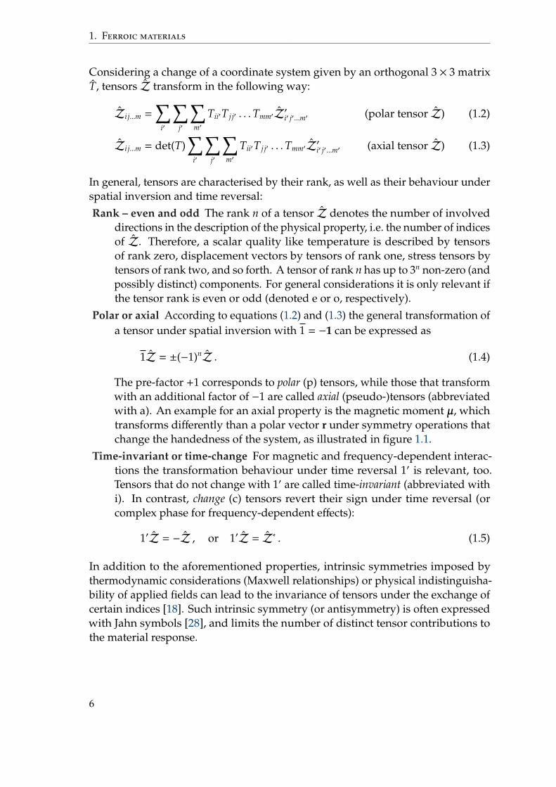
In general, tensors are characterised by their rank, as well as their behaviour underspatial inversion and time reversal:Rank – even and odd The rank n of a tensor Z denotes the number of involved
directions in the description of the physical property, i.e. the number of indicesof Z. Therefore, a scalar quality like temperature is described by tensorsof rank zero, displacement vectors by tensors of rank one, stress tensors bytensors of rank two, and so forth. A tensor of rank n has up to 3n non-zero (andpossibly distinct) components. For general considerations it is only relevant ifthe tensor rank is even or odd (denoted e or o, respectively).
Polar or axial According to equations (1.2) and (1.3) the general transformation ofa tensor under spatial inversion with 1 = −1 can be expressed as
1Z = ±(−1)nZ . (1.4)
The pre-factor +1 corresponds to polar (p) tensors, while those that transformwith an additional factor of −1 are called axial (pseudo-)tensors (abbreviatedwith a). An example for an axial property is the magnetic moment µ, whichtransforms differently than a polar vector r under symmetry operations thatchange the handedness of the system, as illustrated in figure 1.1.
Time-invariant or time-change For magnetic and frequency-dependent interac-tions the transformation behaviour under time reversal 1′ is relevant, too.Tensors that do not change with 1′ are called time-invariant (abbreviated withi). In contrast, change (c) tensors revert their sign under time reversal (orcomplex phase for frequency-dependent effects):
1′Z = −Z , or 1′Z = Z∗ . (1.5)
In addition to the aforementioned properties, intrinsic symmetries imposed bythermodynamic considerations (Maxwell relationships) or physical indistinguisha-bility of applied fields can lead to the invariance of tensors under the exchange ofcertain indices [18]. Such intrinsic symmetry (or antisymmetry) is often expressedwith Jahn symbols [28], and limits the number of distinct tensor contributions tothe material response.
6

1.2. Physical property tensors
Figure 1.3. Form of invariant polar second-rank tensors with intrinsic symmetry χi j = χ ji
for the seven crystal classes (summarising the general symmetry of the 14 translationalBravais lattices). Open circles denote zero, filled circles non-zero contributions. Compo-nents of equal magnitude are connected with lines. The hierarchy of the crystal classes isadapted from [29], and shows the possible continuous deformations from one lattice intoanother.
1.2.2. Anisotropy of material response
It follows from equation (1.1) that the rank and transformation behaviour of amaterial susceptibility Z depend on both the tensor properties of the inducing fieldX and the observableY.The non-zero contributions to Z do not depend on the intrinsic tensor propertiesonly but also on the symmetry group G of the investigated material. This relationshipis summarised by the Neumann principle [18, p. 34]:
“The symmetry of any physical property Z of a crystal must include thesymmetry elements of the point group G of the crystal.”
Therefore, knowledge of intrinsic properties of Z and the point group G is enough todetermine if a physical coupling is allowed by symmetry, and if so, what anisotropythis effect will show. These non-zero contributions can be calculated [25] and aretabulated, e.g. in the book by Birss [16].In general, several scenarios can be distinguished which lead to a vanishing materialresponse, here listed in order of strictest to less strict limitations:
(1) Symmetries of Z and G are incompatible: In this case effects of tensors withthe same symmetry but different rank n′ = n ± 2 are also forbidden. Anexample is the vanishing piezoelectric response (o,p,i) in centrosymmetriccrystals.
(2) The rotational symmetry of G leads to zero contributions: For example, apolarisation P (p,i,o) is allowed in polar materials only. In contrast to theprevious case, higher-order tensors of the same symmetry might be allowed
7

1. Ferroic materials
(e.g. piezoelectric response in non-centrosymmetric non-polar materials).(3) Invariance under symmetric or antisymmetric permutations can also lead to
vanishing contributions of Z. An example is the case of antisymmetric (chiral)contributions χi jk = −χik j to the optical second harmonic response; in contrastthose contributions do not vanish for sum frequency generation which hasthe same tensor properties, but no symmetry under permutation of indices.
(4) Tensor contributions also can vanish accidentally, e.g. due to boundaryconditions or when considering the spectrum of a frequency-dependentresponse. If an effect is allowed by symmetry, however, it usually occurs,which makes the tensor approach so powerful.
In contrast to the previously listed limitations, some material properties are alwaysallowed, for example those described by symmetric polar invariant second-ranktensors χi j = χ ji. Such tensors describe material properties like mechanical stress σ,dielectric ε and magnetic susceptibility µ, or optical birefringence n. Their formonly depends on the crystal class (general translational symmetry) of the materialand therefore the measured anisotropy can also be used to limit the symmetrygroup of an investigated material.4 The general form of such tensors is shown infigure 1.3.
1.3. Ferroic order
The relationship between material symmetry and tensor properties are especiallyuseful when considering phase transitions. In many cases the underlying electricor magnetic long-range order breaks rotational symmetry as well. In this casethe new phase usually has a lower point group symmetry than the parent phase,and as consequence, new tensor properties arise below the critical temperature.Such ferroic phases are technologically relevant, due to their multi-domain states,switchability, and enhanced susceptibilities [30, 31].
1.3.1. Ferroic phase transitions and hysteretic domain switching
As illustrated in figure 1.4 (a) a ferroic phase transition is induced by microscopiclong-range order that is accompanied by a spontaneous symmetry breaking: For auniaxial ferromagnet, the isotropic distribution of the magnetic moments evolvedinto a collinear arrangement below TC. Therefore the isotropy of space as well astime reversal symmetry is broken upon the transition. Consequently, new tensorproperties are allowed to emerge in the ordered phase.
4Tensor properties are usually described in orthogonal (mostly Cartesian) coordinate systemseven if the crystallographic lattice does not feature perpendicular basis translations (such ashexagonal, trigonal, monoclinic, or triclinic lattices).
8

1.3. Ferroic order
Figure 1.4. Defining properties of (a) ferroic phase transitions and (b) ferroic phases forthe case of a uniaxial ferromagnet. (a) The onset of long-range alignment of atomicmagnetic moments below TC breaks the rotational invariance and the time reversal of thematerial. Furthermore, the magnetic susceptibility χ exhibits a strong enhancement nearTC. (b) The observation of a remanent moment MR in zero field and hysteretic switchingdefines a ferroic phase. The field-induced switching process involves the nucleation ofdomains with opposite alignment of the magnetisation M, and the subsequent movementof domain walls. Switching from a multi-domain state (“virgin curve”) is shown in red.
In general, the tensor properties arising below the critical temperature TC canbe macroscopic moments (like a component of the strain tensor, polarisation, ormagnetisation) or a higher-order response function. Related to the microscopicnature of the developing long-range order, the electric and magnetic linear sus-ceptibilities, thermal expansion, and specific heat will show an anomaly at thetransition temperature. The red dashed line in figure 1.4 (a) shows the divergenceof the magnetic susceptibility χ = ∂M
∂H at TC.5
Due to the spontaneous symmetry breaking, two or more degenerate arrangementsare possible in the low-symmetry phase, which are called domain (or twins). Thesedomain states have the same symmetry, magnitude of the ordered property, andenergy, but a different orientation.Figure 1.5 shows the close relationship between the symmetry breaking phasetransition and the occurrence of ferroic domains: The loss of the four-fold rotationaxis 4z of the tetragonal structure in (a) leads to four equivalent structures withlower orthorhombic symmetry group H (b). The rotation 4z transforms thosestates into each other. If the phase transition happens in absence of fields, theseconfigurations are degenerate, and a multi-domain state is expected to arise in theordered phase.The hallmark feature of a ferroic phase is the possibility of aligning and reversingthese metastable states with a suitable applied field, as illustrated in figure 1.4 (b).
5In general, susceptibilities show a divergence (or at least enhancement) at a second-order phasetransition, and a step for first-order transitions. While anomalies in the specific heat (conjugatedto the entropy of a system) are very sensitive to the occurrence of long-range order, describing atransition as first or second order is a more difficult assignment.
9

1. Ferroic materials
Figure 1.5. Symmetry breaking upon a ferroic transition, and distinction between fullyand partially switchable domain states. (a) Depiction of the high-symmetry phase withpoint group G=4/mmm. (b) Loss of the fourfold rotation allows for four degenerateconfigurations with symmetry group H=2/mmm, between which the element 4z transforms(fully ferroic). (c) Loss of the inversion symmetry leads to four polar states with respectivepoint group H′=2mm. Inversion 1 transforms between pairs of domain states only (partialferroic).
The reversal of M → −M costs energy, as domains with opposite magnetisationmust be nucleated and domain walls moved with the driving field. The coercivefield HC is needed to achieve equal domain population; and marks the point wherethe system is continuously driven into a state aligned parallel to the driving field.The example in figure 1.5 shows that the relationship between high-symmetry andlow-symmetry phase also can limit possible switching events: In the transitionfrom (b) to (c) the inversion symmetry is lost. Therefore the domain states nowcan be polar (since point group H′ is polar), i.e. displaying a directed property. Inthis case, however, the inversion operation only relates two domain states to eachother. This relationship limits the possibility to transform a multi-domain state intoa single-domain state by the application of a suitable driving field. This distinctionbetween fully and partial ferroic state shifts was first discussed by Aizu [5, 32].Therefore, knowledge of the point groups of the high-symmetry and ordered phaseallows the prediction of the number, orientation, and possible restrictions on theswitching behaviour of the ferroic domains emerging at the phase transition. Therelationship between different point group symmetries are tabulated, e.g. those byJanovec and Dvorak [33] can be helpful accessing possible low-symmetry phases,while the work by Aizu [5] permits conclusions about the expected switchingbehaviour.The length and time scales that govern the equilibrium and dynamic properties ofdomain patterns are of technological relevance [18, 34, 35]. The switching processalso depends largely on external influences like the sample’s thermal history ordefect concentration. Furthermore, it is important to note that a symmetry-breakingphase transition does not necessitate the emergence of a ferroic state – only theobservation of hysteretic switching behaviour allows us to define a long-rangeordered phase as ferroic.
10

1.3. Ferroic order
1.3.2. Ferroic order parameters and Landau theory
For the mathematical description of the ferroic phase transition it is therefore usefulto find a way to characterise the relationship between high-symmetry and orderedphase. When considering figure 1.5 it can be shown that the combination of allorientations of the domain symmetry groups H restore that of the unordered state G.Therefore, the loss of rotational symmetry upon the transition can be characterisedby the combination of the high-symmetry group G and the transformation behaviourof a so-called order parameter τ, such that G = H ∩ τ holds [17, 36, 37].In general, the transformation behaviour of the order parameter τ can be relatedto an irreducible representation of the parent group G [17, 29]. This concept evenholds when considering phase transitions that are induced by modulated charge orspin order where the breaking of translational symmetry is characterised by a vectorq, which gives direction and periodicity of the modulation in reciprocal space.Fractional values encode an enlargement of the unit cell, while irrational valuesdescribe modulations incommensurate with the underlying ionic lattice [38–40]. Inthis case the irreducible representations τ (or Gq) related to the space group G andthe modulation vector q can have several complex contributions, complicating thephysical description of the system. Irreducible representations are either found intables [23, 41, 42] or can be calculated [37, 43, 44].A description by the combination of a high-symmetry group G and a symmetry-breaking order parameter τ is only possible if the phase transition is continuous,i.e. when the transformation G τ
→ H indeed can be parametrised by infinitesimal“deformations” [17, 43, 45, 46]. This condition is generally obeyed by second-orderphase transitions; and most magnetically-induced transitions (irrespective of beingfirst or second order) also meet this continuity condition.If the transition is indeed continuous, the successful description of the low-symmetryphase(s) requires two more conditions to be met: (1) The choice of the prototypesymmetry group G (para phase), and (2) the choice of the right primary orderparameter.
(1) In some cases, G is chosen to be of higher symmetry than that of the phaseobserved above the critical temperature TC in order to fully explain theproperties of the ordered phase. Figure 1.5 schematically illustrates thispoint: It is more advantageous to describe the transition from (b) to (c) as asubsequent transition from the symmetry shown in (a); only then the full setof domains can be explained successfully.
(2) The primary order parameter τ is the one that fully accounts for the lossof translational, rotational, and time inversion symmetry. Parameters thatcapture the broken symmetry only partly are called secondary order parametersand are especially useful when considering cross-coupling between differentphysical properties.
11

1. Ferroic materials
Figure 1.6. Application of Landau theory for the description of ferroic phases. (a) Theform of the free energy F(τ) is determined by the high-symmetry group G and thetransformation behaviour of the order parameter τ. Minimisation of F(τ) can be usedto determine (b) possible stable states, and their sequence, (c) temperature- and field-dependence of the order parameter and related susceptibilities, and (d) cross-correlations.Furthermore, it is possible to determine the microscopic structure of (e) domains and(f) domain walls and to (g) classify topological defects (illustration of hedgehog defecttaken from [47, p. 199]).
Knowing the parent phase G and the irreducible representations τ, an expansion ofthe Landau free energy can be established: F(τ) only contains those polynomials ofthe order parameter(s) and physical fields which are invariant under the symmetryoperations of G.By assuming that certain pre-factors change sign at TC the spontaneous symmetrybreaking can be explained mathematically. This is illustrated in figure 1.6 (a) whichshows a prototypical free energy above and below the transition temperature: ForT > TC the function F(τ) has only one minimum at τ = 0 equivalent to a non-orderedstate. Due to the sign change of some pre-factor the free energy F(τ) developstwo minima below TC, which determine the equilibrium values ±τ of the orderparameter in the degenerate domain states.The many applications of the symmetry analysis and Landau theory are summarisedin figure 1.6: (b) Minimisation of the free energy permits the determination of thepossible phase transition sequences, stable phases, and their symmetry groups. (c)It also allows the prediction of the (mean-field) temperature- and field-response ofmacroscopic tensor properties and (d) possible cross-couplings terms [17, 37, 43,48]. (e,f) In combination with the ionic description of the material, the symmetryof G and τ imposes constraints on the micro-structure of the domains [43, 49–52]and the domain walls [36, 53]. (g) Considering the configuration space of τ allowsthe classification of possible topological defects related to the symmetry-breakingphase transition [47, 54–56].All the aforementioned arguments underline the usefulness of the strictly mathe-matical approach – even without knowing anything about the exact nature of the
12

1.3. Ferroic order
centro-symmetric
non-centro-symmetric
timeinvariant
timechange
Table 1.7 Primary ferroic order withmacroscopic moment, classified by thetransformation behaviour of the pri-mary order parameter under spatialinversion 1 and time reversal 1′. Here,antiferromagnetic materials breakingboth time and inversion symmetry areof interest. The scheme is adapted from[57] and [58].
microscopic order, the transformation of τ can be calculated and used to predictthe behaviour in the low-symmetry phases.
1.3.3. Classification of ferroic order
So far, the discussion of ferroic materials was based on the symmetry relationshipbetween the high-symmetry and the ordered phase. But the concept of the orderparameters as introduced in the previous section has a physical manifestation onboth microscopic and macroscopic length scales: As discussed before, the loss ofrotational symmetry implies the emergence of new tensor properties below thecritical temperature TC differentiating between the possible degenerate domainstates. The physical nature and symmetry of this macroscopic property and itsbehaviour under applied fields can be used to characterise different kinds of ferroicorder: If a transition is fully characterised by the emergence of a single macroscopicmoment conjugated to mechanical stress or electric and magnetic field, it is calledprimary ferroic order. There are four kinds of primary ferroic states, as shown intable 1.7:Ferroelastics are defined by the emergence of a spontaneous strain which requires
the deformation of the unit cell, i.e. a change in translational symmetry [59–63].Therefore ferroelastic transitions can correspond to changes between two ofthe crystallographic classes as depicted in figure 1.3.
Ferroelectrics develop a spontaneous polarisation that can be switched by anelectric field. As P is a directed property, ferroelectric order is only allowedin non-centrosymmetric, polar materials [64, 65]. Furthermore, usually onlyinsulators or semiconductors are considered as ferroelectric materials, sincein metals the charge dipole would be screened [66, 67].
Ferromagnets show long-range order of the microscopic spin or orbital magneticmoments. While ferromagnets exhibit a collinear arrangement, partially orfully compensated distributions characterise ferri- or antiferromagnetic order,respectively [68–71].
13

1. Ferroic materials
Ferrotoroidic order is defined by the emergence of a macroscopic polar, time-oddtoroidisation T, which can be generated by magnetic vortices [72–77].
In particular, ferroelectric and ferromagnetic materials are of high technologicalrelevance, and are used in many applications. Desirable properties are highsusceptibilities (e.g. for transformers and capacitors), high spontaneous moments(e.g. electro motors), stable domain states (digital data storage), and secondary effectslike pyroelectric and piezoelectric coupling (relevant for sensors and actuators).This classification of ferroic states can be expanded for higher-order tensor prop-erties. In some cases, only the combination of two applied fields can switch thedomain states, which leads to the definition of secondary ferroics [30–32]. As phasetransitions are accompanied in anomalies in temperature-dependent susceptibilitiesand moments, the kind of order can be readily deduced even without knowledgeof what is exactly happening to the material.The microscopic causes for long-range order are related to the local interactionbetween electronic charge, spin, and orbitals, and the ionic lattice. Often it is possibleto generate a relationship between microscopic distortions and the macroscopictensor property related to it. In many cases, however, especially in modulatedphases, the relation between microscopic and macroscopic order parameters is byno means trivial.Multiferroic materials The complexity of the microscopic interactions can leadto the emergence of coexisting ferroic orders, either by subsequent transitions ofdifferent character, or due to strong intrinsic cross-coupling of the different micro-scopic degrees of freedom. Such materials showing the simultaneous occurrenceof different long-range order are called multiferroic [78]. The terminology is notrestricted to bulk materials, but is also used for thin films and heterostructuresespecially interesting for technical applications [58, 70, 71, 79–86].In this thesis especially the coexistence of both magnetically and electrically orderedstates and possible cross-coupling to applied fields is of interest. In particular, itwas shown that magnetically modulated spin-spiral materials allow for intrinsiccross-coupling terms leading to magnetically induced ferroelectricity.As discussed in the next chapter and the main part of the thesis, those materialsoffer a variety of possibilities to affect the electric properties by magnetic fields.Many of the observed effects are not yet fully understood; especially a pictureembracing all length scales – microscopic, mesoscopic, and macroscopic – is stillmissing.
14

2. Spin-spiral multiferroic andmagnetoelectric materials
Spin-spiral multiferroics are characterised by the occurrence of a magnet-ically induced spontaneous polarisation. The electric properties of suchmaterials can often be tuned by applied magnetic fields, and this chapteraims to give an overview of the vast possibilities of microscopic andmacroscopic cross-couplings. The prerequisites of modulated magneticorder, as well as the symmetry constraints and microscopic interactionsallowing for the emergence of ferroelectricity are discussed.
The observation of cross-correlations between electric and magnetic properties ofcrystals are generally termed as magnetoelectric couplings. The archetype for suchan interaction is the linear magnetoelectric effect, where a polarisation is inducedby a magnetic field, and vice versa:
P = αHH , and M = αEE . (2.1)
The intrinsic linear magnetoelectric effect was first predicted and measured forCr2O3 [87–89]: Here, the antiferromagnetic order breaks both inversion symmetryand time reversal, and therefore allows non-zero contributions to the tensor α.Generally, the term magnetoelectric includes all kinds of cross-couplings betweenelectric and magnetic properties, which come in a surprising variety, as will bediscussed in detail in section 2.3. The relevance of such effects are extensivelydiscussed for multiferroic materials: In theory, the possibility to affect a spontaneouspolarisation (magnetisation) of a crystal with a magnetic (electric) field offers manyopportunities for technological applications [58, 70, 71, 79–81, 85].But the coexistence of magnetic and electric long-range order does not necessitatea strong cross-coupling: In many materials, polarisation and magnetic orderoriginate from different microscopic mechanisms, and thus only weak interactionsare expected to arise. This is different in so-called spin-spiral ferroelectrics, where amodulated spin order induces a spontaneous dipole moment: While the polarisationis usually several orders of magnitude weaker than in “conventional” ferroelectricmaterials, it can often be strongly affected by a magnetic field. Examples are themagnetic-field-induced polarisation reorientation in TbMnO3 [90], or the magnetic-field-induced suppression of the net polarisation in TbMn2O5 [91].
15

2. Spin-spiral multiferroic and magnetoelectric materials
Curiously, the reverse effect of manipulation of a magnetisation M(E) by an electricfield is much more difficult to achieve. This is due to the fact that E only breaksspatial inversion and not time reversal, so that the coupling to the magneticproperties can only happen via indirect means [71, 85, 86, 92–99].Most of the spin-spiral multiferroics observed so far are oxides with magnetictransition-metal or rare-earth ions. The following chapter reviews the mainingredients leading to complex modulated spin order, and the symmetry argumentsand microscopic interactions required to allow for a spontaneous polarisation.Finally, the influence of the magnetic field on the microscopic spin order and themagnetically induced polarisation is discussed.
2.1. Magnetism in transition-metal oxides
Transition-metal oxides show a remarkable versatility for tuning the correlationsbetween the lattice, charge, spin, and orbital degrees of freedom. This broadnessenables complex phases which are susceptible and controllable with applied fields,and therefore of profound technological interest. Examples are high-temperaturesuperconductivity, quantum criticality, giant magneto-resistance [7, 100–102],spintronic applications [6, 84, 99, 103], and magnetoelectric multiferroics [58, 78,80].The structure of many transition-metal oxides consist of a close-packed lattice ofoxygen ions, as O2− usually has the largest ionic radius. The metal cations are placedon some (or all) of the interstitial sites. The magnetic ions are therefore surroundedby oxygen polyhedra, and the interaction with the low-symmetry environmentstrongly affect the electronic, magnetic, and optical properties [104–106]. Due to thelimited screening of the 3d states these effects related to the crystal-field splittingare especially pronounced for transition metal ions of the iron series.The ionic and electronic structure of such materials can promote competing magneticinteractions, and strong correlations between electronic spin, charge, orbitals andthe underlying atomic lattice. Therefore, semiconducting transition-metal oxideswith localised 3d (and 4 f ) moments allow for strong intrinsic cross-couplings thatpossibly lead to multiferroic and magnetoelectric behaviour.Considering the magnetic order, the spatial distribution of spins is mainly governedby two energy scales: First, exchange interactions between magnetic momentsstipulate the overall spatial modulation. Second, the spin orientation is mainly gov-erned by the local environment of the ion which determines the magnetocrystallineanisotropy. The symmetry and properties of the magnetic structure therefore aresensitive to the balance of these interactions in relation to temperature and appliedfield.
16

2.1. Magnetism in transition-metal oxides
Figure 2.1. The magnetic exchange is sensitive to the bond angles between oxygen O (red)and metal ion M (grey): (a) Edge-sharing polyhedra enforce the angles ∠(M-O-M) to beclose to 90◦, which leads to weakly ferromagnetic exchange, while (b) corner-sharingpolyhedra promote larger bond angles and stronger antiferromagnetic interactions.1
(c-h) Connectivity networks for different spin-spiral materials [108]: Open and solidcircles mark ions differing by element, sites symmetry, or valency. Single and doublelines mark connections via corner- and edge-sharing oxygen polyhedra. Dashed linesconnect next-next-nearest neighbouring ions. (c) RMn2O5 [109], (d) MnWO4 [110], (e)olivine Mn2GeO4 [111], (f) o-RMnO3 [90], (g) delafossite CuFeO2 [112], (h) Ni3V2O8 [113].
2.1.1. Magnetic exchange interactions
Curiously, the strongest interaction between magnetic ions often does not originatefrom dipolar interactions between the spin S or orbital L moments, but rather dueto quantum mechanical exchange interactions based on the interplay of the Pauliprinciple and electrostatic Coulomb repulsion [68, 69, 71, 107].Super-exchange interactions The leading-order term to interactions between mag-netic ions in transition-metal oxides is due to super-exchange: Here, the ions ondifferent sites interact via the orbital overlap with one (or several) oxygen p orbitals.Phenomenologically, the exchange Hamiltonian can be written as
HHeisenberg = −Ji jΣSi · S j . (2.2)
Considering this term, only the relative orientation of the spins Si, j matters but nottheir absolute direction in space. The largest energy contributions are expectedfor collinear spin arrangements ↑↑ or ↑↓. Which of these two configurations isfavoured depends on the sign of the exchange integral Ji j. This constant dependson the occupation and the overlap of all involved d and p orbitals. Therefore, signand strength of the super-exchange interactions are strongly anisotropic in space.The relationship between orbital occupation, M-O-M bond angle, and favouredspin arrangement is summarised in the Goodenough-Kanamori-Anderson (GKA)
1These and all following crystallographic structures were rendered with VESTA [114].
17

2. Spin-spiral multiferroic and magnetoelectric materials
rules [107, 115–117]. These rules give a rough relation between the connectivity ofmetal ions with ferromagnetic or antiferromagnetic exchange paths: Bond angles∠(M-O-M) close to 90◦ are expected to be weakly ferromagnetic, while straighterM-O-M bonds promote strong antiferromagnetic interactions.Frustrated interactions The GKA rules are valid for next-nearest (NN) neighboursonly. But exchange between ion pairs of larger distance can be strong, too, especiallyif the NN interactions are weak. The overall spin structure therefore is determinedby the competition between all exchange paths. This can lead to situations whereno spin structure can simultaneously satisfy all magnetic interactions. Sucharrangements usually occur for interactions between an odd number of ions,competing interactions between nearest- and next-nearest neighbours, or structuresof low dimensionality [118–120]. Figure 2.1 shows the connectivity networks ofsome materials that promote magnetic frustration.There are four main ramifications of frustrated interactions: (1) The transition into along-range ordered state occurs for critical temperatures TN or TC much lower withrespect to the Curie-Weiss temperature obtained from the magnetic susceptibility.2
(2) The occurrence of modulated magnetic order. (3) Ground-state degeneracy,which allows for competing phases and the possibility to influence the magneticstructure by an applied field. In the case of very strong frustration, this competitioneven prevents long-range order to occur.Spin spirals A common consequence of strong frustration are long-range modulatedmagnetic structures, or in the broadest sense, spin spirals. Such configurationsare characterised by a modulation vector q describing the magnetic periodicity inreciprocal space. If the magnitude of q does not correspond to a rational fraction ofthe crystallographic lattice, the emerging incommensurate modulation breaks theoverall translational symmetry. As a result, the order parameter describing themodulation has several complex contributions; and can allow for further symmetrylowering and cross-correlations to occur.
2.1.2. Magnetocrystalline anisotropy
The symmetry of the magnetic phases do not depend on the modulation vector qonly, but also on the direction of the local moments, which is determined by themagnetocrystalline anisotropy [68, 69].The main contribution to magnetocrystalline anisotropy is the single-ion term,which is governed by the shape of the electronic orbitals (given by the angularmomentum L), the local charge distribution around the crystallographic site, andthe strength of the spin-orbit interaction.
2The Néel temperature TN gives the critical temperature of an antiferromagnet, while the Curietemperature TC marks the transition into a ferromagnetic (ferrimagnetic, ferroelectric) phase.
18

2.2. Spin-induced ferroelectrics
Mathematically, the single-ion anisotropy can be expressed as
Haniso = SiKSi , (2.3)
with the symmetric and traceless anisotropy tensor K. Depending on the sign of thenon-zero contributions the local moment will align along an easy axis or easy plane.Large anisotropy energies, as usually found for 4 f ions [69], imply that it is difficultto affect the spin order with a magnetic field applied along a “hard” direction.The situation is slightly different for 3d ions: Stronger interaction with the sur-rounding ions leads to the (partial or full) quenching of the orbital moment. This,and the fact that the transition-metal ions are lighter, means that the spin-orbitcoupling is not as effective as for example for rare-earth ions. As a consequence,for transition-metal oxides the anisotropy energy is usually much lower thanthe exchange interactions. Furthermore, the local orientation of the 3d magneticmoments cannot be concluded as simply as for the 4 f ions. On the other hand,the smaller anisotropy energy offers more versatility to form complex magneticstructures.
2.2. Spin-induced ferroelectrics
While ferromagnetic materials show long-range ordering of the microscopic mag-netic moments, ferroelectric materials are characterised by the emergence of a spon-taneous polarisation due to charge displacements. Therefore, both effects are usuallynot coupled. Some materials, however, show simultaneous (antiferro-)magneticand ferroelectric order, where the latter is induced by the former. Such couplingterms are especially promoted in materials with complex modulated spin order.The presence of magnetically induced ferroelectricity depends on both the sym-metry breaking generated by the onset of magnetic order, and on the microscopicinteractions between spin, orbital, and lattice degrees of freedom.
2.2.1. Macroscopic symmetry of spin-spiral order
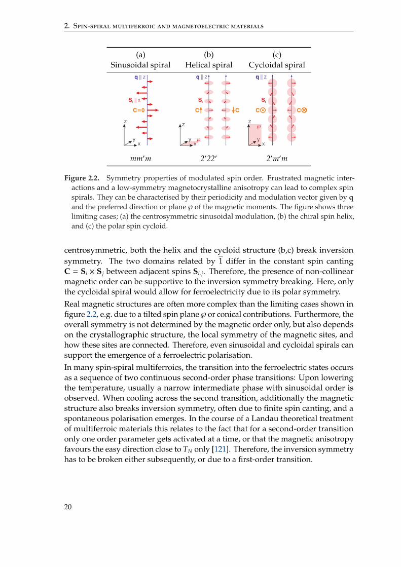
As discussed in section 1.3.3, ferroelectric behaviour can only be observed inmaterials with polar point group symmetry. Therefore, to get a magneticallyinduced polarisation, the spin order has to break spatial inversion symmetry.The symmetry properties of modulated magnetic structure are summarised infigure 2.2 which shows three archetypical spin spirals. They are characterisedby the propagation vector q, and the preferred direction or plane ℘ in which themagnetic moments are modulated.A symmetry analysis of the magnetic spirals allows the determination of theirrespective point symmetry group: While the sinusoidal spiral in figure 2.2 (a) is
19
2. Spin-spiral multiferroic and magnetoelectric materials
(a) (b) (c)Sinusoidal spiral Helical spiral Cycloidal spiral
mm′m 2′22′ 2′m′m
Figure 2.2. Symmetry properties of modulated spin order. Frustrated magnetic inter-actions and a low-symmetry magnetocrystalline anisotropy can lead to complex spinspirals. They can be characterised by their periodicity and modulation vector given by qand the preferred direction or plane ℘ of the magnetic moments. The figure shows threelimiting cases; (a) the centrosymmetric sinusoidal modulation, (b) the chiral spin helix,and (c) the polar spin cycloid.
centrosymmetric, both the helix and the cycloid structure (b,c) break inversionsymmetry. The two domains related by 1 differ in the constant spin cantingC = Si × S j between adjacent spins Si, j. Therefore, the presence of non-collinearmagnetic order can be supportive to the inversion symmetry breaking. Here, onlythe cycloidal spiral would allow for ferroelectricity due to its polar symmetry.Real magnetic structures are often more complex than the limiting cases shown infigure 2.2, e.g. due to a tilted spin plane ℘ or conical contributions. Furthermore, theoverall symmetry is not determined by the magnetic order only, but also dependson the crystallographic structure, the local symmetry of the magnetic sites, andhow these sites are connected. Therefore, even sinusoidal and cycloidal spirals cansupport the emergence of a ferroelectric polarisation.In many spin-spiral multiferroics, the transition into the ferroelectric states occursas a sequence of two continuous second-order phase transitions: Upon loweringthe temperature, usually a narrow intermediate phase with sinusoidal order isobserved. When cooling across the second transition, additionally the magneticstructure also breaks inversion symmetry, often due to finite spin canting, and aspontaneous polarisation emerges. In the course of a Landau theoretical treatmentof multiferroic materials this relates to the fact that for a second-order transitiononly one order parameter gets activated at a time, or that the magnetic anisotropyfavours the easy direction close to TN only [121]. Therefore, the inversion symmetryhas to be broken either subsequently, or due to a first-order transition.
20

2.2. Spin-induced ferroelectrics
2.2.2. Microscopic magnetoelectric interactions
On a microscopic scale a number of models relate the emergence of ferroelectricbehaviour to the spin-spiral order [83, 108, 122–125]. Common for all mechanismsis the magnetically-induced modulation of bond length or bond angles, or redis-tribution of electronic orbitals, leading to a global imbalance of the distributionof negative and positive charges. The effectiveness of these couplings depend onmany parameters, such as the valence of the magnetic ion, its magnetic moment,site symmetries, the strength of spin-orbit coupling, and the hybridisation withligands.In many cases it is not clear whether lattice or electronic contributions play the majorrole for the ferroelectricity: Spin-induced polarisation values are usually in theorder of 1µC/m2 to 1000µC/m2. Ionic shifts necessary to generate this magnitudeof P are in the order of 10−3 Å, and thus difficult to detect with diffraction methods[126–128]. The distinction between purely ionic or electronic contributions probablyis not entirely necessary anyhow, as cross-relaxation will occur.Ferroelectricity due to non-collinear magnetic order In many spin-spiral multifer-roics ferroelectricity is a consequence of non-collinear magnetic order, and the signof the polarisation is directly coupled to the spin chirality C = Si × S j [129–131].This coupling between magnetic order and ferroelectric polarisation can eitherbe explained by the Dzyaloshinskii-Moriya interaction [132–134], or via the spin-current mechanism [135, 136]. In the former case, the interaction between non-collinear spins can lead to ionic displacements stabilising the magnetic structure [137,138]. The latter model relates the spin current between non-collinear neighbouringspins js ∝ C with the polarisation P, as both have the similar symmetry properties.On a phenomenological level, the coupling terms have the same form, but the spin-current model is allowed for any local symmetry, while the Dzyaloshinskii-Moriyainteraction vanishes for centrosymmetric metal-oxygen clusters.Overall, antisymmetric exchange strongly depends on the strength of spin-orbitcoupling, as was demonstrated nicely by the ferroelectric properties of Ru-dopedMnWO4: The 4d ions allow for stronger LS coupling, which enhances the sponta-neous polarisation by almost an order of magnitude [139].Ferroelectricity due to collinear magnetic order Breaking of spatial inversion doesnot necessary involve a finite spin chirality. The symmetry of the ionic structureor the superposition of two sinusoidal spin-density modulations can also lead topolar structures [121, 140]. Here, instead of being proportional to the off-centring ofions, the non-zero polarisation is related to the magnetically-induced dimerisationof inequivalent bonds or sites [122, 141]: Inequivalent ionic occupation can forexample be achieved by the presence of sites with distinct local symmetry or bycharge-ordered states of ions differing in element of valency. Magnetic order alsocan generate inequivalent bonds, e.g. the configuration ↑↑↓↓ exhibits alternating
21

2. Spin-spiral multiferroic and magnetoelectric materials
Figure 2.3. Different ways to affect a dipole moment with a magnetic field: (a) Field-induced polarisation; (b,c) enhancement or suppression; (d) sign reversal, or flip; (e)discontinuous 90◦-rotation, or flop; (f) continuous rotation.
ferromagnetic and antiferromagnetic bonds [138, 142, 143].For charge-ordered magnetic states, ferroelectric polarisation contributions bothparallel and transverse to the modulation vector can emerge. The forces betweendifferent ions originate either from superexchange (exchange striction [144], leadsto P ⊥ q) or double exchange interactions (for mixed ionic valency, induces P||q).Therefore they do not depend on the absolute spatial orientation of the spins. Asspin-orbit coupling is not involved, in general these mechanisms might inducelarge polarisation values for collinear spins [141], especially if the M-O-M bondsare not completely straight [108].On-site dipole moments The previously discussed cross-coupling terms are in-duced by the interaction between neighbouring spins. In addition, on-site polarisa-tion contributions also can be of interest. Here, due to metal-ligand hybridisationthe direction of the local spin can affect the bonding strength. This, in turn, maylead to local displacements [142, 145–148]. A net polarisation can arise if the metalsite is non-centrosymmetric [149] and the spin order is non-collinear [150]. Themagnitude of this effect depends on factors like single-ion anisotropy, pd orbitaloverlap, and spin-orbit coupling strength.The underlying metal-oxygen hybridisation leads to the spin-polarisation of theinitially non-magnetic ligand, which is known to affect both spin-independent andspin-dependent properties on the connected sites [138, 151]. The induced momenton the oxygen site can have sizeable magnitude, and was found in a number ofmultiferroic and magnetoelectric materials [152–155].
2.3. Polarisation control by a magnetic field
Due to the close relationship between magnetic order and spin-induced ferroelec-tricity, significant magnetoelectric coupling can be expected in spin-spiral materials.Indeed, the magnetic field can lead to a multitude of changes in both magnitudeand direction of the net polarisation, as illustrated in figure 2.3.In the last ten years numerous examples for such cross-coupling effects were found,
22

2.3. Polarisation control by a magnetic field
(a1) P(H) ∝ HLiFeSi2O6 [156]Cr2O3 [88, 89]GaFeO3 [157]
(a2) P(H) ∝ f (H2)Cu2OSeO3 [158, 159]Ba0.52Sr2.48Co2Fe24O41 [85]Sr3Co2Fe24O41 [160]ZnCr2Se4 [161]
(a3) field-induced polar phaseNi3TeO6 [98]CuFeO2 [162]
(b) P(H) > P(0)DyMn2O5 [163]HoMn2O5 [164]CuBr2 [165]Ni3V2O8 [166]
(c) P(H) < P(0)TbMn2O5 [91]ErMn2O5 [164]Ba2Mg2Fe12O22 [167]α-CaCr2O4 [168]CaMn7O12 [169, 170]Ni3V2O8 [166]HoFe3(BO3)4 [171]
(d) P(H) = −P(0)Mn2GeO4 [172]CoCr2O4 [173]GdFeO3 [174]Lu2MnCoO6 [175]MnWO4 [176, 177]
(e) P(H) ⊥ P(0)MnWO4 [178]o-TbMnO3 [90]o-DyMnO3 [179]LiCuVO4 [180]TmMn2O5 [181]YbMn2O5 [182]LiCu2O2 [183]
(f1) P(φ) ∝ HMn0.95Co0.05WO4 [184]Ba2CoGe2O7 [185]
(f2) P(φ) ∝ H(φ)Ba0.5Sr1.5Zn2Fe12O22 [186]Eu0.75Y0.25MnO3 [187]Ba2Mg2Ge12O22 [188]CuFe0.965Ga0.035O2 [189]
Magnetoelectric and multiferroic materials investigated in this thesis compriseYMn2O5 & TbMn2O5 [190] (chapter 4), Mn0.95Co0.05WO4 (chapter 5), Mn2GeO4
(chapter 6), Cu2OSeO3 (together with MnSi & Fe0.8Co0.2Si, appendix A) andMnWO4 (appendix B).
Additionally investigated, but not discussed here: CaBaCo2Fe2O7 [191], CuO[192], InMnO3 [193], LiFeSi2O6.
Table 2.4. Examples of materials showing the magnetoelectric couplings illustrated infigure 2.3. Some multiferroics can exhibit several cross-couplings dependent on fieldorientation and magnitude. Subcategories are listed for (a) magnetic-field-inducedpolarisation contributions with initial P(0) = 0, and an induced polarisation rotation by(f1) a magnetic field with fixed direction, or (f2) a rotating magnetic field.
23

2. Spin-spiral multiferroic and magnetoelectric materials
underlining the versatility of strong correlations between magnetic and electricproperties in modulated spin-spiral materials. Table 2.4 gives an overview ofmaterials allowing for the magnetic-field control of an electric polarisation.The general magnitude and effect of interactions between spin-spiral materials andmagnetic fields depends on the subtle relationship between intrinsic degrees offreedom, like exchange interactions, magnetic anisotropy, spin-orbit coupling, andspin-dependent hybridisation.In general, the prevalent strong antiferromagnetic exchange interactions prohibitthe easy deformation of the spin spiral, and often relatively high field strengthsare required to induce magnetoelectric effects. However, materials with a smallmagnetisation, e.g. due to conical spiral order or rare-earth moments, were shownto be more susceptible to magnetic-field-induced changes of the polarisation [90,91, 188].Regarding the classification of field-induced effects three main causes can bedistinguished: First, magnetoelectric coupling can arise due to field-induced phasetransitions, or the shift of transition temperatures due to an applied magnetic field.Second, field-induced contributions can be induced by the reversible deformationof the overall magnetic structure. Third, magnetoelectric interactions can alsobe enabled by the direct coupling in ferroic domains and domain walls. Theconsequences of each cause are briefly discussed in the following section.
2.3.1. Field-induced phase transitions
Regarding magnetic phase transitions, an applied field can have two consequences:First, if the magnetic structure is characterised by successive phases a field mayfavour one of these over the other. In turn, the ferroelectric properties associatedwith each phase will also change with the shift of the transition temperature, for ex-ample leading to magnetic-field-induced polarisation enhancement or suppression.This effect can allow for gigantic magnetoelectric couplings, due to the delicatebalance of magnetic structures and phase coexistence at a morphotrophic phaseboundary [90, 98, 163].Second, additional symmetry-breaking phase transitions induced by a magneticfield can occur. Such meta-magnetic transitions are characterised by the suddenreorientation of the local moments. This new macroscopic symmetry frequently doesnot have a direct relationship with the zero field arrangements symmetry, inducinga first-order phase transition, and can result in new magnetoelectric couplings.This will change both magnitude and direction of the induced polarisation.Polarisation flop The most common example of such meta-magnetic reorientationare spin-flop transitions: Strong antiferromagnetic interactions will counteract withthe field-induced magnetisation, especially if the field is applied along the magnetic
24
2.3. Polarisation control by a magnetic field
easy axis. When the magnetocrystalline anisotropy is weak, this frustration can beovercome by the reorientation of the magnetic moments perpendicular to the fieldwhile still mostly satisfying anti-parallel alignment which maximises the isotropicexchange energy [68].Regarding the magnetoelectric cross-coupling, this spin-flop model successfullyexplains the sudden reorientation of the net polarisation in materials like MnWO4
[178], o-TbMnO3 [90], o-DyMnO3 [179], or LiCuVO4 [180]. In these materials, thepolarisation is a consequence of a cycloidal spiral as shown in figure 2.2 (c). Atsufficient magnetic field the spin-spiral plane changes by 90◦; which leads to thesimultaneous reorientation of the polarisation direction.In principle, these first-order reorientation transitions can lead to a new arrangementof domains [194], especially if the number of domain species increases. Thetorque that the magnetic field will apply on the spin spiral is the same, however,independent on the handedness present in the magnetic domains, which can leadto a preservation of the domain state upon the flop transition [195]. In addition, thedegeneracy of the domain states can be lifted by a slight canting of the magneticfield, so that the initial and flopped domain distribution often coincide [196–198].
2.3.2. Field-induced polarisation contributions
Apart from sudden changes, an applied magnetic field also continuously deformsthe microscopic spin structure, which leads to elliptical and conical variants of thespirals shown in figure 2.2. The field-induced changes in macroscopic symmetryand local spin configuration influence the microscopic coupling and thus can leadto changes in the net polarisation [199]: Phenomenologically, the macroscopicdipole moment can thus be described as a sum of polarisation contributions withparallel or distinct direction and field-dependence, coupling to different aspects ofthe microscopic spin order.These contributions induced by the continuous and reversible deformation of themicroscopic spin structure often show either linear or quadratic behaviour withthe applied field or field-induced magnetisation.3 Therefore, such effects do notshow a hysteresis, and the zero-field arrangement can be restored fully.Depending on how the microscopic spin order is affected, the polarisation contribu-tions decrease or increase with the magnetic field, e.g. by reducing antiferromagneticcorrelations, or increasing the effective spin canting. Furthermore, ions with com-peting local anisotropies can lead to a constant rotation of a spin-spiral plane
3The modulated spirals shown in figure 2.2 do not break macroscopic time reversal, therefore donot allow a linear magnetoelectric coupling term as expressed by equation (2.1). The presence ofa finite magnetisation due would, in principle, allow for non-zero coupling.
25

2. Spin-spiral multiferroic and magnetoelectric materials
– in turn, the polarisation will also reorient. Such a situation, reminiscent of acontinuous spin flop, was observed in Mn0.95Co0.05WO4, for example [184].
2.3.3. Cross-coupling between ferroic domains and domain walls
Phase transitions and field-induced polarisation contributions affect the wholesample in the same way, even if the sign of the polarisation differs in the distinctferroelectric domains. Apart from irrevocable changes accompanying a first-ordertransition these effects are expected to be fully reversible.This is different for magnetoelectric cross couplings that involve the interactionbetween ferroelectric and ferromagnetic domains and domain walls. In this case,coupled hysteretic switching of both magnetisation and polarisation is possible, asobserved for CoCr2O4 [173], Mn2GeO4 [172], and Lu2MnCoO6 [175].The permanent changes of the ferroelectric properties caused by a magnetic fieldcan therefore allow for the persistent cross-control of the multiferroic domain states,of interest for technical applications [79, 200].Even if both a spontaneous polarisation and magnetisation are present in a material,in most cases they are not directly coupled, and cross-switching is not possible –this is a more complex analogue to the partial and full ferroic switching discussed insection 1.3.1. Because in spin-spiral multiferroics both M and P originate from thesame antiferromagnetic structure, more elaborate cross-couplings can be allowed.Furthermore, the local spin order at the multiferroic domain boundaries can leadto phenomena not present in bulk [201], and can enable couplings to external fields[202, 203], too. Controlling the properties of localised interfaces between domainsallows for additional multifunctionalities which extends the technological potentialof ferroic domain states [204]. In turn, the presence of magnetoelectric domainwalls can also affect bulk properties: The ferroelectric polarisation in CoCr2O4 is, forexample, thought to be due to the field-induced movement of multiferroic domainboundaries [205]. In addition, the role of 90◦-boundaries stabilising the domainpattern before and after spin-flop transitions have been discussed [197, 206].Overall, most experiments on multiferroic materials do not consider the interactionson mesoscopic length scales, nor the magnetic-field dependence of the ferroelectricdomain population determining the net polarisation. Therefore, especially themagnetoelectric interactions discussed here are not fully understood yet, since thedirect observation of ferroelectric and magnetic domains is only possible with alimited number of experimental techniques.
26

2.4. Open questions & thesis outlook
2.4. Open questions & thesis outlook
As illustrated in the previous section, there exist a number of multiferroic materialswhich allow diverse magnetoelectric couplings. The cross-correlation betweenmagnetic structure and the spontaneous polarisation is usually investigated withintegrating methods – like pyroelectric current measurements – sensitive only to thenet polarisation dependent on the applied field. Microscopic probes, like neutronand resonant x-ray scattering, Mössbauer spectroscopy, and muon spin rotation,give insight into the local structure. In combination, macroscopic and microscopicmeasurement methods often allow the development of a model which relates theobserved effects on both length scales.There are some limitations, since macroscopic methods cannot distinguish betweendistinct collinear contributions to the net polarisation, nor gather information aboutthe mesoscopic domain distributions and how they are affected by magnetic fields.It is therefore desirable to use an experimental technique that permits both thedistinction of different order parameters and the imaging of ferroic domains. Inthis thesis, three examples of magnetoelectric multiferroics were investigated withoptical second harmonic generation, which is a symmetry-sensitive technique idealfor investigating ferroelectric phases and cross-couplings.This integrated approach reveals the behaviour of distinct polarisation contribu-tions in YMn2O5, TbMn2O5 and Mn0.95Co0.05WO4, while SHG domain imagingelucidates the magnetoelectric coupling at ferroelectric domains and domain wallsin Mn0.95Co0.05WO4 and Mn2GeO4.
27


3. Non-linear optics
A material can exhibit a non-linear optical response if intense lightfields are used. Of particular interest for the investigation of ferroicmaterials is the generation of a second harmonic wave with twice theinitial photon energy: This response is sensitive to the material symmetry,and therefore allows the background-free coupling to structural andmagnetic long-range order. Due to the many experimental degrees offreedom, and the possibility to access macroscopic, mesoscopic, andmicroscopic scales, SHG is a superior technique to investigate ferroicmaterials and field-induced phenomena, and especially suited in itsapplication to multiferroic and magnetoelectric materials.
Non-linear optical excitations were first discussed by Maria Göppert-Mayer in1931 [207], but it was with the invention of the laser in 1960 by Maiman [208] thatfacilitated the high-power and intense light fields required to investigate thesephenomena in more detail [209, 210].Nowadays, materials with non-linear optical absorption and emission are usedin many technical applications such as laser sources with tunable frequency [211,212], up-converting phosphors [213–215], photonic devices [216], solar cells withenhanced quantum efficiency [217], and many more [218].In this thesis second harmonic generation (SHG), or optical frequency doubling,is used to investigate ferroic transitions and phases. This process, sketched infigure 3.1, describes the simultaneous absorption of two photons with the sameenergy ~ω and the direct re-emission of a photon with 2~ω. Excitation and non-linear response are closely linked by the symmetry of the material, and thus SHGcan be used to detect changes at symmetry-breaking phase transitions in bulkmaterials, surfaces, and even buried interfaces [219–222].This chapter introduces the theoretical concepts of second harmonic generation andexplains the symmetry selection rules relevant for the observation of ferroic phases(sections 3.1 to 3.3). The experimental setup used for the following experimentsis outlined briefly in section 3.4. Section 3.5 explains the general experimentalcharacterisation of non-linear signals, followed by details about the investigationsof ferroic materials in section 3.6.
29

3. Non-linear optics
Figure 3.1 Schematic illustration of the SHG process: Two photons ofenergy ~ω are virtually absorbed and induce the emission of a photon withtwice the initial energy 2~ω. Due to the coherent nature of the process,the polarisation dependence of the SHG excitations is determined by thesymmetry of the material.
3.1. Optical second harmonic generation (SHG)
In a simplified picture, light-matter interaction is caused by the vibration of electronsin matter as response to the external light field. Due to the anharmonicity of theelectronic potential, an incident light wave of sufficient strength can induce higher-order vibrations in a material, which act as emitters of light with higher (or lower)frequency.1 In the following, we consider only the simplest non-linear processwith degenerate light fields E(ω), and thus investigate the production of the secondharmonic wave with 2ω = ω + ω.Using the Maxwell equations the higher-order excitations can be expressed in termsof the incident light field with polarisation E(ω) and momentum k(ω).2 The derivedsource term S(2ω) will act as a source for light emission at 2ω [224, 225]:
S(2ω) = µ0∂2P(2ω)∂t2︸ ︷︷ ︸ED
+µ0 ∇ ×∂M(2ω)∂t︸ ︷︷ ︸
MD
−µ0∂2(∇ · Q(2ω))
∂t2︸ ︷︷ ︸EQ
. (3.1)
The three terms correspond to electric and magnetic dipole (ED, MD) or electricquadrupole (EQ) contributions to the induced non-linear oscillation of the lightfield S(2ω). Considering only terms quadratic in the electric field component of thelight field, their anisotropic dependence on E(ω) and S(2ω) can be expressed bytensor equations [226]:
P(2ω) = ε0 χnlED(2ω,ω)E(ω)E(ω) ,
M(2ω) = ε0c0n(ω) χnl
MD(2ω,ω)E(ω)E(ω) ,Q(2ω) = −icε0
2ωn(ω) χnlEQ(2ω,ω)E(ω)E(ω) .
(3.2)
Therefore, the characterisation of the hyperpolarisability tensors χnlED, χnl
MD, and χnlEQ
can give insight into the symmetry of a material. In particular, the leading-orderelectric dipole term P(2ω) is allowed in systems with broken inversion symmetry
1The vibration in an anharmonic potential is nicely illustrated in [223, ch. 11].2The vector k(ω,E) gives the propagation direction of the light within the material. Its magnitude
is given by |k(ω,E)| = nωc0
with energy- and polarisation-dependent refractive index n = n(ω,E).
30

3.2. Symmetry selection rules
SHG tensor symmetry restriction for non-zero χ
i-ED (p,o,i) non-magnetic non-centrosymmetric (1 broken)c-ED (p,o,c) broken 1 and 1′ (but 1′ can be symmetry element)MD (a,o,i) noneEQ (p,e,i) none
EFISH (p,e,i) noneMFISH (a,e,i) neither 1 nor 1′ is a symmetry element
Table 3.2. Symmetry of different SHG tensors and the requirements for the crystallographic(and magnetic) point group of the material permitting these effects. In this thesis, we payparticular attention on c-ED SHG induced by spin-spiral multiferroic order.
only. Therefore, SHG is a suitable experimental technique to investigate surfaces,interfaces, and ferroelectric phases [222, 227], where the signal arises free ofbackground contributions. Furthermore, it can be used to study antiferromagnetictransitions, field-induced effects, and even carrier transport.The intensity of the observable second harmonic light is proportional to the normsquare of the (complex) source term in equation (3.1). As light is a transverse wave,only the second-harmonic light field S⊥(2ω) ⊥ k(ω,E) perpendicular to the lightpropagation direction k(ω,E) has to be considered for the measured SHG response:
ISHG(2ω) ∝ |S⊥(2ω)|2 (3.3)
In addition, the SHG yield of a tensor contribution χi jk(2ω,ω) depends strongly onthe electronic structure and the linear optical properties of the material, as brieflydiscussed in section 3.3.
3.2. Symmetry selection rules
Due to the tensor relationships described in equation (3.2) a close correlationexist between the polarisation directions of E(ω), S(2ω) and the crystallographicdirections of the investigated material. As described in section 1.2 such a linkwill limit the non-zero contributions of the material tensor describing the physicaleffect.3 General properties of the non-linear hyperpolarisability tensors – like rankand behaviour under inversion and time reversal – are given in table 3.2. Incombination with the material point group symmetry, they determine the non-zero
31

3. Non-linear optics
contributions of χ, which can be looked up in tables, e.g. in the work by Birss [16].Usually, for non-centrosymmetric materials a strong non-linear optical response isexpected; while MD and EQ terms of non-leading order are allowed for centrosym-metric materials, too. Their signal strength is usually about two or more ordersof magnitude lower than that of i-ED SHG4 but can have similar amplitude to thec-ED SHG induced in magnetic phases [231].In the case of electric dipole SHG, the observation of a modulated polarisation-dependent SHG intensity (discussed in more detail in section 3.5.4) can be directlylinked to the excited ED tensor contributions:
SEDi (2ω) ∝ Pi(2ω) , with Pi(2ω) = χED
i jk (2ω,ω)E j(ω)Ek(ω) . (3.4)
Due to the spatial derivatives in equation (3.1) the polarisation dependence S(2ω)of the MD and EQ non-linear terms additionally depend on the light propagationdirection k(ω): The magnetic dipole term contributes as a cross product with k(ω),while the quadrupole term is given by a contraction of the EQ tensor with the lightpropagation vector:
SMDi (2ω) ∝ εi jkk jMk(2ω) , with Mk(2ω) = χMD
klm (2ω,ω)El(ω)Em(ω) , (3.5)
SEQj (2ω) ∝ kiQi j(2ω) , with Qi j(2ω) = χEQ
i jkl(2ω,ω)Ek(ω)El(ω) . (3.6)
Therefore, the assignment of MD and EQ tensor contributions to the observedsignals must be approached with more prudence than that of ED contributions.In many cases the polarisation dependence given by SMD(2ω) and SEQ(2ω) is thesame, and thus MD and EQ tensors (most often giving a temperature-independentbackground signal) cannot be distinguished – for the same (magnetic) pointsymmetry group their polarisation dependence is usually different to that of i-EDSHG, and at most times distinct to c-ED SHG, too [16].
3.2.1. Field-induced SHG response
In addition to SHG due to the crystallographic structure, additional non-linearsignals can arise when symmetries are broken by extrinsic fields or internal long-range order.
3In an experiment with collinear incident light fields the degeneracy of E(ω) leads to up to eighteenχi jk that can be distinguished for ED or MD SHG (and up to 54 distinct χi jkl for EQ SHG). Aconsequence of the particular tensor symmetry χi jk = χik j is that chiral contributions χxyz = −χxzy
cannot be observed with SHG [228–230], but only with sum frequency generation (SFG).4The derivation of the source term contributions contain spatial derivatives for MD and EQ SHG
as in equation (3.1). Due to the ratio between light wavelength and crystallographic latticeconstants those contributions are usually two orders of magnitude weaker than crystallographicED-SHG signals.
32

3.2. Symmetry selection rules
In the case of electric-field induced SHG (abbreviated EFISH) the application ofa static electric E(0) field removes the macroscopic inversion symmetry, and thusadditional SHG contributions are allowed:
S(2ω) ∝ χEFISH(2ω,ω)E(ω)E(ω)E(0) (3.7)
To detect EFISH contributions, the electric field (or a projection of it) has to be appliedperpendicular to the light propagation direction k(ω). Such an induced effect canbe distinguished by material-specific SHG due to its quadratic field-dependenceIEFISH(2ω) ∝ |E(0)|2 [232, 233].Conversely, an applied magnetic field also can generate a second harmonic ex-citation (abbreviated MFISH) dependent on the static (induced or spontaneous)magnetisation M(H(0)). The material response is given by the equation
S(2ω) ∝ χMFISH(2ω,ω)E(ω)E(ω)M(H(0)) , (3.8)
and is allowed in non-centrosymmetric systems only. Usually it has a differentpolarisation dependence than i-ED SHG and thus can be distinguished from thecrystallographic non-linear response. Therefore, MFISH signals can be used toinvestigate the behaviour of magnetised bulk materials and interfaces [219, 220,234–238].Since charge currents break both spatial inversion and time reversal symmetry,transport properties can be investigated with SHG as well [239–242]. Such ex-periments are especially interesting for the contact-free detection of spin currents[135], as discussed and observed in spintronic materials [243, 244] and topologicalinsulators [245–247].
3.2.2. Coupling to ferroic order parameters
Due to its inherent sensitivity to symmetry breaking, SHG is a superb techniqueto investigate ferroic transitions and phases. Most commonly it is used to studyferroelectric materials [222, 227, 248], but it also allows to investigate antiferromag-netic and magnetoelectric materials [220, 221]. In particular, it is one of the fewexperimental techniques that allow the imaging of antiferromagnetic 180◦-domains,as first shown for Cr2O3 [231, 249, 250].As described in chapter 1 ferroic transitions are characterised by the loss ofpoint group symmetry elements. Therefore, new non-linear susceptibility tensorcontributions coupling to the primary and secondary order parameters are expectedto arise below the critical temperature TC.If the transformation behaviour of the order parameters is known, an extendedtensor approach can be used to predict the ferroic non-linear contributions [251].In most cases, however, it is enough to compare the form of the SHG tensors
33
3. Non-linear optics
in the high- and low-symmetry phase to determine contributions coupling toferroic order parameters. In particular, for transitions from centrosymmetric tonon-centrosymmetric phases a pronounced SHG signal coupling to the inversion-symmetry breaking of the microscopic order is expected to arise. For ferroelectricmaterials usually only those ED-SHG contributions χi jk(2ω,ω) are non-zero wherethe tensor indices i jk contain an odd combination of the polar direction ‖ P.5
In the case of spin-spiral ferroelectrics, SHG usually couples only to translational-invariant combinations of the complex order parameter, and it often cannot bedistinguished if the non-linear response originates from the magnetism or thepolarisation. Although optical methods are usually insensitive to the breaking oftranslational symmetry, the occurrence of magnetic order with incommensuratelymodulated moments can lead to non-zero SHG contributions as well [252].The assignment of SHG contributions to macroscopic order parameters is usuallydone on a purely phenomenological assumption on the basis of temperature- andfield-dependent measurements (see also section 3.6). Due to the spectroscopic andpolarisation degree of freedom of SHG it is possible to observe independent orderparameters simultaneously [253–255]
3.3. Spectral dependence of SHG yield
The selection rules discussed in the previous section only determine if a non-linearresponse is allowed in a material, but not if and at what photon energies 2~ω theyoccur and which intensity the SHG excitation will have. There are three factors thatlargely affect the magnitude of the non-linear signals: the electronic structure of thematerial, as well as the linear optical properties, namely absorption and refraction.Especially interesting for the investigation of transition-metal materials are crystal-field excitations of magnetic 3d ions, which usually occur in the infrared to ultravioletspectral range [106, 256, 257] and can allow for SHG signals coupling to the long-range magnetic order. Furthermore, due to the different selection rules for linearand non-linear transitions, SHG spectroscopy can be used as a complimentary toolto determine the electronic structure of a material [258, 259].Electronic structure A quantum mechanical perturbation theory treatment of thenon-linear excitations reveal that if real electronic states are in the vicinity of theenergies ~ω or 2~ω the SHG yield can be resonantly enhanced [218, 260–262].This is illustrated in figure 3.3 (a) with states |i > and |e > near the incident anddoubled photon energy. On a phenomenological level this relationship is alsoexpressed by Miller’s rule [263], which relates the complex linear dielectric response
5The only exception to this rule are materials with trigonal and hexagonal symmetry, which allowadditional SHG contributions, tabulated in [16].
34
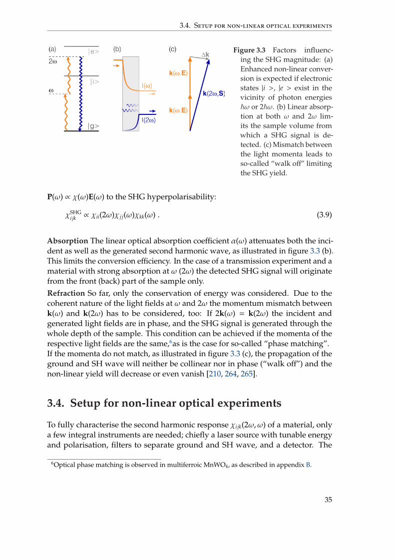
3.4. Setup for non-linear optical experiments
Figure 3.3 Factors influenc-ing the SHG magnitude: (a)Enhanced non-linear conver-sion is expected if electronicstates |i >, |e > exist in thevicinity of photon energies~ω or 2~ω. (b) Linear absorp-tion at both ω and 2ω lim-its the sample volume fromwhich a SHG signal is de-tected. (c) Mismatch betweenthe light momenta leads toso-called “walk off” limitingthe SHG yield.
P(ω) ∝ χ(ω)E(ω) to the SHG hyperpolarisability:
χSHGi jk ∝ χii(2ω)χ j j(ω)χkk(ω) . (3.9)
Absorption The linear optical absorption coefficient α(ω) attenuates both the inci-dent as well as the generated second harmonic wave, as illustrated in figure 3.3 (b).This limits the conversion efficiency. In the case of a transmission experiment and amaterial with strong absorption at ω (2ω) the detected SHG signal will originatefrom the front (back) part of the sample only.Refraction So far, only the conservation of energy was considered. Due to thecoherent nature of the light fields at ω and 2ω the momentum mismatch betweenk(ω) and k(2ω) has to be considered, too: If 2k(ω) = k(2ω) the incident andgenerated light fields are in phase, and the SHG signal is generated through thewhole depth of the sample. This condition can be achieved if the momenta of therespective light fields are the same,6as is the case for so-called “phase matching”.If the momenta do not match, as illustrated in figure 3.3 (c), the propagation of theground and SH wave will neither be collinear nor in phase (“walk off”) and thenon-linear yield will decrease or even vanish [210, 264, 265].
3.4. Setup for non-linear optical experiments
To fully characterise the second harmonic response χi jk(2ω,ω) of a material, onlya few integral instruments are needed; chiefly a laser source with tunable energyand polarisation, filters to separate ground and SH wave, and a detector. The
6Optical phase matching is observed in multiferroic MnWO4, as described in appendix B.
35

3. Non-linear optics
Figure 3.4. Schematic experimental setup for SHG experiments. Polarisation optics (GT,λ/2, in red) allow the control of the incident ground wave E(ω) and the analysis ofthe SHG response S(2ω) of the sample. Incident and generated light are separatedusing suitable filters (F1,F2) and detected with a CCD camera or a photomultiplier (PM).Further details are discussed in section 3.4.
investigations in this thesis were mainly performed in a transmission setup asshown in figure 3.4. Reflection experiments with small-angle or 90◦ incidence canbe done with a similar setup. In the following the optical components shown infigure 3.4 are discussed, while details about the sample environment are describedin section 3.6.1.Illumination A coherent laser source is needed for non-linear optical experiments,which can be achieved by a combination of a pulsed laser with frequency mixingstages and a tunable optical parametric amplifier or oscillator (OPA, OPO). Thisallows the covering of spectral ranges from the near infrared to the ultraviolet.7
The higher peak electric fields obtained for shorter femtosecond pulses also permitreflection experiments on surfaces and thin films. In contrast, nanosecond pulseshave a higher pulse energy, larger beam diameters, and a flatter spectrum.Polarisation control The selective excitation of SHG contributions χi jk(2ω,ω) canbe achieved by controlling E(ω) and S(2ω) separately: A Glan-Taylor prism (GT)sets the initial laser polarisation E(ω) (i.e. the laboratory frame with vertical andhorizontal polarisation), which can then be rotated by an achromatic λ/2-waveplate in a motorised mount. To analyse the SHG polarisation S(2ω) a rotatableGlan-Taylor prim is placed behind the sample. The rotational anisotropies of SHGsignals are further discussed in section 3.5.4.Signal separation To avoid damage on the optics and the detection of additionalnon-linear signals, a high-pass filter (F2) is directly placed behind the sample(Schott). It absorbs most of the incident light field at ω. Sometimes, additionalinterference filters can be used (Melles-Griot). A low-pass filter (F1) in front of thesample removes the strong SHG signals produced by the Glan-Taylor prism andthe wave plate.
7Two systems were used here: One, a nanosecond Nd:YAG laser (1064 nm, 7 ns, ContinuumPowerlite Precision II) in combination with a optical parametric oscillator (GWU Versa Scan).Two, an amplified femtosecond Ti:sapphire laser (800 nm, 120 fs, Coherent) in combination withan optical parametric amplifier (Coherent TOPAS).
36
3.5. Observation and characterisation of SHG signals
Detection The generated SHG intensity can be detected either with a photomulti-plier or a CCD camera, which additionally allows spatially resolved measurements.In general, signal acquisition with a photomultiplier and a gated integrator allowsfast detection and a good signal-to-noise ratio even for small signals.8 Liquid-nitrogen cooled CCD cameras with high quantum efficiency can also detect smallSHG signals with good spatial resolution.9 By integrating over a chosen region(track) non-imaging experiments can also be performed (furthermore, both modescan be combined). The use of a monochromator (MC) allows the enhancement ofthe spectral resolution.Additional optics The sample illumination can be controlled with lens L1, whilelens L2 is used either to collimate the beam (if it is divergent) or to image the sampleonto the CCD detector. Their position can be fine-tuned by placing the lenses ontranslation stages.
3.5. Observation and characterisation of SHG signals
The aim of the following section is to describe the experimental steps for findingand characterising the SHG response of a material: Linear optical spectra givean indication of interesting spectral regions. By scanning the in these ranges,higher-order excitations can be found. The source of these signals needs to beverified to be due to SHG, and then characterised by their energy and polarisationdependence given by χi jk(2ω). The use of this signal to investigate ferroic phasesand domains is explained in section 3.6.
3.5.1. Linear absorption and reflection spectra
As indicated by Miller’s rule in equation (3.9), there exists a relationship between thelinear and non-linear response of a material. By measuring absorption or reflectionspectra, regions containing dd-transitions appearing as peaks or shoulders canbe identified [106]. Those features can also depend on the magnetic order of thematerial [256, 257] and may allow for a non-linear response coupling to the ferroicorder parameters. On the other hand, high absorption limits the SHG yield, asshown in figure 3.3 (b) and decreases the optical damage threshold of the sample.10
8When using a photomultiplier the applied high voltage and the sensitivity of the electronicsshould be chosen such that the relationship between incoming SHG intensity and generatedelectronic signal is linear. Photomultipliers are inherently sensitive to applied magnetic fields,and their use in high fields is limited.
9Two brands of CCD cameras with 256 × 1024 pixels per chip are available: Photometrics CH270(26.0µm × 26.2µm pixel size) and Horiba Jobin Yvon Symphony (20.0µm × 19.9µm pixel size).
10If the absorption is too high either the measurements have to be performed in reflection geometryor the sample has to be thinned accordingly.
37

3. Non-linear optics
Linear optical spectra presented in this thesis were measured with the microspectrometer MSV-370 by Jasco. The microscope can select the sample volumewhere optical density O.D., transmission T, and reflection R of the sample ismeasured. A spectral range of 190 nm to 2500 nm is covered (photon energies0.5 eV to 6.5 eV). The relationship between measured sample properties O.D. andT and material-specific absorption coefficient α is given by
1 − T = 10−O.D. = e−αd⇒ α =
ln(10) O.D.d
, (3.10)
with sample thickness d. More precise measurements also account for reflectionlosses at the sample surfaces [266]. The general use (and certain pitfalls) of themicro spectrometer are described in the instrument manuals and in [267]; here Ijust wish to point out a few remarks about polarisation-dependent measurements.Angular dependencies One can measure the angular polarisation dependence ofthe absorption (or reflection) at a fixed photon energy by successively rotating thepolariser, e.g. in 5◦ or 10◦ steps.11 As the detection efficiency is highly dependenton the light polarisation, one has to measure an angular baseline: The absorptionvalues at a fixed photon energy ~ω are measured for all polariser angles firstwith the sample, and then without. Subtracting these values gives α(φ). Suchan experiment only takes a few minutes, therefore, thermal fluctuations of thespectrometer will not likely disturb the measurement.Circularly polarised light To investigate chiral materials with optical activity [268–270], or directions of high symmetry like three-, four-, or six-fold axes or cubic facesit is advisable to work with circularly polarised light.12
To measure absorption or reflection spectra with circularly polarised light oneattaches an achromatic λ/4-wave plate behind the spectrometer polariser. If theoptical axis of the wave plate is vertical (l), polarisation angles of 0◦ and 90◦ ( ↔, ↔ )will lead to left- and right-circularly polarised light. For both settings new baselineshave to be measured.Spectrum analysis A useful tool to analyse absorption spectra is the "Peak Analyser"routine of OriginLab [271]. Before analysing the absorption peaks it is a goodidea to subtract the high-energy background, which is usually either a transitionacross the band gap Eg with the absorption behaving like α(ω) ∝
√~ω − Eg [223]
or a metal-oxygen charge-transfer transition with α(ω) behaving like a Gaussian(or Lorentzian) peak. This ensures that transitions hidden in the absorption edgeare also found. Assignments to crystal-field dd transitions can be made usingTanabe-Sugano diagrams [104–106]; information about charge-transfer excitationsare for example found in [106, 272, 273].11Such an angular dependence of the absorption coefficient is shown for Mn2GeO4 in figure 6.4.12Reflecting the high symmetry, only four SHG contributions are distinguished when working with
circularly polarised light, which are χ+++, χ+−−, χ−++, and χ−−−. Optical activity with α+ , α−was observed for chiral Cu2OSeO3 (see appendix A.3).
38

3.5. Observation and characterisation of SHG signals
3.5.2. Non-linear spectroscopy
As explained in section 3.3, the SHG response is especially enhanced for photonenergies ω or 2ω near electronic transitions of the material. Also, as selection rulesfor one- and two-photon processes are different, SHG peaks can also be found atenergies not obvious from the linear spectra.Non-linear spectra are measured by tuning the incident photon energy ~ω whiledetecting the signal at 2~ω (ω-2ω spectrum). When a CCD camera is used, thespectral range is limited by the detector sensitivity and the filter transmission.Better spectral resolution is achieved by using a monochromator, which detectssignals at 2ω synchronous to the laser tuning frequency ω.The experimental coordinate system is given by the light propagation vector k(ω)and two orthogonal polarisation directions in the plane perpendicular to k.13 Ifnothing is known about the non-linear properties of a material, the six distinguish-able ω − 2ω spectra should be investigated.14 Often higher-order excitations arefound in energy regions for which the linear spectra show distinguished featuresas shoulders or peaks.For quantitative comparison of non-linear spectra e.g. for different energy ranges,other sample directions, or materials the measurements have to be normalised.This is usually performed by dividing the sample response by a reference surfaceSHG signal, e.g. from a silver mirror [274].15
3.5.3. Tests for SHG
For short laser pulses and high photon energies other higher-order optical interac-tions can compete with the SHG response of a material [214, 215]. Other two- ormulti-photon excitations can be distinguished by a true second harmonic responseby employing several tests:Power dependence Since SHG is a two-photon process its intensity ISHG(2ω) scaleswith the square of the input power P(ω); or more accurately with [218]
ISHG(2ω) = P(ω) tanh2(c√
P(ω)) . (3.11)13Together with the intrinsic symmetry of the SHG process only six contributions can be distin-
guished in a given sample setting (four if circularly polarised light is used). The relation betweenthe non-linear susceptibility tensor of the material as described in section 3.2 and that of thegiven sample setting is obtained by transforming the tensor between the different coordinatesystems using equations (1.2) and (1.3).
14If the sample is mounted such that the principal in-plane directions are not known, the first runof NLO spectra can be made by arbitrarily using horizontal and vertical light polarisation. Oncea non-linear signal is found, polarimetry measurements reveal the direction of the in-plane axes.
15If the SHG reference sample is mounted in the same position as the sample the normalisationaccounts for all linear absorption properties of the setup (however, the polarisation dependenceof the monochromator still has to be accounted for).
39

3. Non-linear optics
The power dependence of a non-linear signal can be measured by attenuating theincident beam with grey filters. ISHG(P) should appear as a line with slope equal (orsmaller) than 2 in a double-logarithmic plot. Steeper slopes point to higher-orderoptical excitations, and therefore exclude SHG as the signal origin [275].Spectral position and width A second harmonic signal should appear at exactlytwice the incident photon energy. This can be checked using an interference filteror doing a monochromator scan.16 In particular, a central energy lower than 2~ωindicates a process involving energy transfer between real electronic states [214,276].Symmetry dependence The materials symmetry constrains the possible non-zerocontributions χi jk(2ω,ω) and thus determines the polarisation dependence of thenon-linear signal. Therefore, a clear rotational anisotropy obeying the symmetryselection rules discussed in section 3.2 is a sign of a SHG response. This behaviour isespecially evident for symmetry-breaking transitions; a signal coupling to a ferroicorder parameter and vanishing above the critical temperature TC is most likelydue to SHG. Deviations from the aforementioned symmetry selection rules and inparticular an isotropic polarisation dependence points to higher-order fluorescencenot due to SHG.Coherence and decay time The aforementioned criteria can only be used toexclude other non-linear excitations, but not to unambiguously confirm that asignal originates from SHG only. Even coherence is not a unique feature of SHG incomparison with other non-linear optical processes [216, 277]. A stringent test forSHG would be the observation of the signal decay time, which must be zero due tothe virtual nature of the process. In contrast, the occupation of real states impliesexponential decay after the exciting light field is switched off.
3.5.4. SHG Polarimetry
An anisotropic polarisation dependence ISHG(φ) of an SHG signal reflects thenon-zero contributions χi jk(2ω,ω) of the hyperpolarisability. On one hand, thisanisotropy can be used to restrict the possible point group of the material. If thesymmetry is already known, ISHG(φ) can be used to determine the crystallographicaxes in the plane perpendicular to k(ω).17
Figure 3.5 shows the rotational anisotropies generated by exemplary SHG contri-butions: Here, polar plots show the modulated SHG intensity with the (relative)rotation of the sample between parallel (S(2ω)||E(ω), anisotropy 0◦) and perpendic-ular (S(2ω) ⊥ E(ω), anisotropy 90◦) polarisation of incident and induced light.16The central transmission frequency of an interference filter can be slightly shifted by tilting it.17The discussion in this section is mainly valid for experiments in transmission geometry, and
small-angle reflection. For observation under large reflection angles usually this formalism nolonger works, so s, p, and d polarisations (given by the lab frame) are usually used [278].
40

3.5. Observation and characterisation of SHG signals
χvvv χvhh χvvh
Polarization of lightfields E(ω) and S(2ω)
Anisotropy 0◦
E(ω)||S(2ω)
Anisotropy 90◦
E(ω) ⊥ S(2ω)
Figure 3.5. Angular dependence of selective excitation of single ED-SHG contributionsχi jk, with vertical and horizontal light polarization, v and h, respectively. The upper rowshows the light fields involved in exciting χi jk, the lower row the rotational anisotropiesoriginating from such contributions. The light polarisations involved in exciting χvvh canalso induce a response from other non-zero contributions. The behaviour of the otherthree possible contributions χhhh, χhvv, and χhhv is obtained by interchanging h↔ v, i.e.,rotating the diagrams by 90◦.
The measurement of rotational anisotropies can quickly discern the number andrelative magnitude of non-zero SHG contributions, as well as determine theorientation of the two primary orthogonal axes of the material in the planeperpendicular to k(ω). A rotation of the sample with respect to horizontal andvertical axes is accounted for by an offset angle φ0.If more than two contribution are simultaneously excited in the anisotropy measure-ments, relative amplitudes and phase can be determined by additional rotationaldependencies acquired from polariser or analyser experiments: In the first case,S(2ω) is fixed to lie along the in-plane axes, while E(ω) is modulated. If thesemeasurements do not complete the picture, rotating the analyser while E(ω) is fixedto lie along or in-between the axes gives additional information.The angular modulation of the SHG intensity can be related to the materialsymmetry in two steps: First, the allowed SHG contributions (see section 3.2) canbe expressed in the chosen coordinate system by using the tensor transformationsin equations (1.2) and (1.3).Sine and cosine functions give the in-plane projectionsof the light fields and can be used to model the angular modulation.18
For example, an angular dependence of an analyser measurement (fixed E(ω)) can
18Figure A.5 and table A.6 shows the result for symmetry group 231′.
41

3. Non-linear optics
be described by the following general term:
I(φ) = |A cos(φ − φ0) + Beiθ sin(φ − φ0) |2 . (3.12)
Due to the coherent superposition of two terms, interference occurs. As a con-sequence, more complex patterns with rotated lobes, lost mirror symmetry, andadditional dips can occur. Often, the phase angle in eiθ can be chosen to be either 0or π (corresponding to pre-factors of ±1).
3.6. Investigation of ferroic phases
Due to the symmetry breaking at a ferroic transition, new SHG contributionsare expected to arise, as explained in section 3.2.2. Here, magnetoelectric andmultiferroic materials with broken inversion symmetry are of particular interest.A route to finding background-free SHG signals coupling to the ferroic orderparameter is to compare non-linear spectra in the ordered and the high-symmetryphase. Contributions only present in the low-temperature phase point to secondharmonic generation. Such signals have to be verified to be SHG using the testfrom section 3.5.3 and analysed by their polarisation-dependence (discussed insections 3.2 and 3.5.4).These signals then can be used to investigate the domain distribution, and thebehaviour of the material under varying temperature and applied electric ormagnetic fields. The following sections briefly explain the control of the sampleenvironment, and imaging of ferroic domains with SHG.Small and large SHG contributions Some experiments require the simultaneousobservation of SHG signals with magnitudes differing by two to three orders ofmagnitude.19 Different contributions to the non-linear susceptibility can only besuccessfully separated if they have a distinct polarisation or spectral dependence.If such signals are measured in the same experimental run, the sensitivity of thedetector20 should be chosen such that neither the large signal saturates (and possiblydamages) the electronics nor the small signal disappears in noise.
19For example, in RMn2O5 (chapter 4) and Mn0.95Co0.05WO4 (chapter 5) both large and smallSHG signals differing by two orders of magnitude were observed. In both cases they could bemeasured independently due to their perpendicular polarisation dependence of the SHG light.
20Detector sensitivity here means either the combination of photomultiplier high voltage andsensitivity of the gated integrator, or the binning of the CCD track. Care should also be takenthat the detectors are not overexposed.
42

3.6. Investigation of ferroic phases
3.6.1. Sample environment
Interesting ferroic transitions and magnetoelectric properties in bulk materialsare most commonly observed at low temperatures. Therefore, all experiments inthis thesis were performed in a cryogenic environment provided by the use of amagnet cryostat (Oxford Spectromag 4000): A superconducting coil allows theapplication of magnetic fields |µ0H| up to 7 T in either Faraday (k||H)21 or Voigt(k ⊥ H) configuration. The hysteresis of the magnet upon field sweeps is typicallyless than 5 mT. The sample is mounted to a sample rod which is placed in avariable temperature insert (VTI); cooling is done via thermal exchange with Hegas with controlled flow and temperature [279].Sample preparation Optical linear and non-linear transmission experiments usuallyrequire thin samples with flat surfaces to avoid unnecessary losses due to absorptionor scattering. Although the materials investigated in this thesis were grown indifferent research groups the sample preparation was usually done on site. Singlecrystals are oriented using Laue x-ray diffraction, and then cut with either an innerdiameter or a diamond wire saw. The resulting platelets are lapped to thicknessesof 50µm to 500µm, and their surfaces are polished by chemical-mechanical orpurely mechanical processes [280–282].Sample mounting For experiments at cryogenic temperatures the samples have tobe glued to an intermediate mount, which then is attached to the sample rod. Fortransmission experiments, mounts are either drilled copper plates, Teflon cubes, ortransparent glass slides.22 Samples can be attached with various adhesives, likesilver paste, textile tape, glue threads,23 or vacuum grease.24 Mechanical stressdue to thermal expansion or protruding ridges can lead to cracks; therefore it isadvisable to sand down the edges of drilled holes and to attach only two or threecorners of the sample.Temperature-dependent measurements The temperature-dependence of the SHG
21For large magnetic fields and light in the visible range, rotation of the light polarisation due tothe Faraday effect in the cryostat windows have to be accounted for.
22Alternatively, a sapphire substrate can be used – the material is transparent, centrosymmetric,electrically insulating, and exhibits excellent thermal conductance. In experiments with trans-parent substrates it is advisable that the side with the sample faces the detection unit – in thiscase the generated signal is not attenuated.
23With this method the sample can be clamped to a mount: With a sharpened toothpick one takes afresh ball of UHU Hart and dips it first into acetone to prevent drying and then onto the mountsurface to anchor it. Thin glue threads can be drawn and fixed similarly on the other side of thesample. It takes a "network" of threads to fully secure the sample position.
24A thin layer of vacuum grease on a glass slide is especially suitable for very small samples thatcannot be mounted with other means [193]. Provided no air bubbles are trapped below thesample even SHG imaging experiments are possible. Normal vacuum grease (Dow Corning"High vacuum grease") freezes out at −100 ◦C (leads to a dimpled pattern in imaging), whilelow-temperature vacuum grease does not (Apiezon Grease N).
43

3. Non-linear optics
intensity often allows a phenomenological connection to be made to macroscopic(primary or secondary) order parameter(s) known from integrated measurementor neutron scattering. Transition temperatures obtained by SHG measurementsusually differ from literature values because of the effects of thermal coupling inthe cryostat and the accumulative heating from the laser radiation. The intensityvariation ISHG(T) reflects both the temperature dependence of the order parameterit is coupling to, as well as the change in linear optical properties. As the latter isknown to vary across phase transitions [256, 257, 269, 283, 284] SHG contributionsnot vanishing above the critical temperature have to be accessed carefully.
3.6.2. Application of electric fields
To switch a ferroelectric domain state an electric field conjugated to the spontaneouspolarisation must be applied. This is achieved by placing the sample betweenconducting electrodes, one to which a voltage is applied while the other is connectedto the ground. The central electric field can be calculated using the equation E = U/dwith applied voltage U and electrode distance d.Therefore, the magnitude of the maximal field Emax is limited by both the voltagesupply (here, high voltages up to 4 kV were used), the minimum distance of theelectrodes (50µm to 5 mm), and electrical break-through. The last effect is enhancedfor materials with leaky conductance or high defect concentration, asymmetric orsharp-edged electrodes, and reduced He gas pressure.Metal electrodes A convenient design uses metal electrodes, which resemble steelcuboids with rounded and polished edges. Specially built plastic holders forhorizontal or vertical electrode arrangement are available for the cryostat samplerods. The ends of the high-voltage cables can be squeezed between metal andplastic to ensure the electrical connection. Cube-shaped samples can be wedgeddirectly between the pole shoes, while thin platelets are best glued to a Teflon cubewith a conical hole of suitable size, and then placed between the electrodes.ITO electrodes Smaller distances and thus higher electric fields can be achieveusing conducting indium tin oxide (ITO) layers. The second advantage of usingtransparent ITO electrodes is that the electric field can also be applied in the beamdirection E||k. Here, the sample can either be sandwiched between separate ITOlayers, or the electrodes can be grown directly on the sample with pulsed laser
44

3.6. Investigation of ferroic phases
Figure 3.6. Detection of ferroic 180◦-domains with SHG imaging: (a) Across the domainwall, the ferroic order parameter Γ changes sign, and consequently the SHG contributionχ ∝ Γ does, too. As only the net intensity is measured, the domains appear withequal brightness, while destructive interference leads to black lines at positions of thedomain wall. The width of the black wall reflects the imaging resolution rather thanthe dimensions of the ferroic domain boundary. (b) If a constant (crystallographic orinduced) background signal is present, interference with the ferroic contribution leads todifferent brightness levels between domains. This contrast can be used to determine thephase of an order parameter.
deposition (PLD).25 To apply electric fields, thin gold wires are attached to the ITOelectrodes and the high voltage cable with (heavily diluted) silver paste. If thesample is very thin and very high electric fields are required it is advisable to use adielectric material to insulate the front and rear side of the sample.26
General remarks Sparks to the VTI housing can be prevented by covering theends of the high-voltage cables and part of the electrodes with Kapton tape. It isadvisable to take a photo of the installed sample before insertion – it helps to assignthe direction of the electric field. Thermal coupling can be rather bad because ofthe bulkiness of the plastic sample holder, and large temperature shifts can occur.
3.6.3. SHG imaging
Spatially resolved measurements of the SHG contributions coupling to the ferroicorder parameters can image the domain distribution in the sample.
25For the ITO growth the sample has to be fixed on a glass slide (e.g. by glue threads) and theelectrode area masked – for this I used a piece of Kapton tape and cut out a rectangle of suitablesize. Alternative ways to mask and attach the sample must sustain the PLD growth temperatureof 120 ◦C, and avoid shadowing effects due to a masking layer of uneven thickness. Since theas-grown ITO layer has a brownish colour, the sample has to be annealed at suitable hightemperature (two hours at 580 ◦C under O2 atmosphere). ITO acts as an anti-diffusion barrier,thus the material properties are not expected to change due to the high-temperature treatment.Comparison of optical spectra before and after annealing can give a hint if the physical propertieshave changed due to the thermal treatment.
26For room-temperature experiments nail polish works well, for cryogenic temperatures vacuumgrease is an alternative. If the grease is not uniformly attached SHG imaging is not possible.
45

3. Non-linear optics
Different lenses can be used to image the sample onto the detector; camera objectivelenses offer achromatic imaging with little aberration, while normal lenses permitfor easy handling. The minimal working distance is determined by the dimensionsof the cryostat, and usually limit the magnification factor to not exceed 5.27 Thespatial resolution is determined by the optics and the wavelength of light, andgenerally limited to 1µm.The illumination of the sample and the quality of the imaging can roughly bechecked by using linear light or the SHG signal of the half-wave plate (by removingthe low-pass filter in front of the sample). Especially for imaging with a femto-second laser it is advisable to use an interference filter directly in front of the CCDto avoid detecting additional fluorescence signals.Domain imaging If the domain size is large enough, SHG imaging with a signalcoupling to the corresponding order parameter can detect the distribution andanisotropy of the ferroic domain pattern. A good indicator that confirms theobservation of domains are changes after heating and cooling cycles across thecritical temperature, or with applied fields.Depending on what signals are additionally excited, two general scenarios haveto be distinguished, as illustrated in figure 3.6: Either opposite domains appearwith equal brightness separated by a black line, or, when interference is present,as areas of different brightness. The constant reference signal can be an intrinsiccrystallographic or field-induced SHG contribution, or externally induced in aquartz crystal [287, 288].As discussed in figure 3.3 (b) absorption at ω and 2ω limits the volume of which aSHG signal is observed. If the sample is thin compared to the typical size of ferroicdomains, usually no interference of different domains along the optical path willoccur. In this case even a rotation of the sample within the beam (e.g. to exciteadditional SHG contributions) can image the in-plane domain distribution.Analysis of domain properties Domain patterns can be analysed by their lengthscales, anisotropies, and textures. These properties are determined by the under-lying microscopic interactions, defect distribution, and macroscopic stray fieldsas well as the thermal history of the sample [18, 34, 35, 289]. Speckled domainpattens are usually interpreted as a sign of small-scale domains with sizes belowthe resolution limit, however they can also appear due to other reasons.28
The analysis of large sets of domain images can be automated using MatLab scriptsas briefly explained in appendix C.
27Higher magnifications and a limited depth resolution can be achieved with special microscopicobjectives with large working distance or by using SHG scanning methods [285, 286].
28In Mn0.95Co0.05WO4 the SHG contribution χbbb leads to the observation of a speckled patternalthough both χbaa and χabb showed the distribution of well distinguishable ferroelectric domainsof moderate size (see section 5.5).
46

Part II.
Polarization controlwith magnetic fields
In many spin-spiral multiferroics the magnetic field allows to controlmagnitude, orientation, and sign of the spontaneous polarisation, asillustrated below. In the following chapters three prototypical examplesof such cross-coupling effects are investigated.
Optical second harmonic generation can probe these phenomena indetail, and can uncover the field-dependence of both the macroscopicpolarisation and the ferroelectric domain distribution:
In chapter 4 the observation of independent polarisation contributions un-derlines the importance of the rare-earth moment to the magnetoelectriccoupling in TbMn2O5 and YMn2O5.
In chapter 5 the continuous magnetic-field induced polarisation rota-tion in Co-doped MnWO4 is used to demonstrate an unprecedentedconfiguration control of the multiferroic domain boundaries.
In chapter 6 the coupled reversal of both magnetisation and polarisationin olivine Mn2GeO4 is investigated, with special focus on the field-response of the ferroelectric domain pattern.
47


4. Rare-earth-induced polarisationsuppression in TbMn2O5
Multiferroic TbMn2O5 shows a pronounced magnetoelectriceffect as even moderate magnetic fields can suppress and evenrevert the sign of the ferroelectric polarisation. To explain thisunusual coupling, models with two independent contribu-
tions adding up to the observed net polarisation were proposed – byusing the versatility of non-linear optics, indeed several contributions tothe net polarisation in TbMn2O5 could be separated by second harmonicgeneration.Here, this analysis was extended to investigate the magnetic-field de-pendence of the ferroelectric polarisation in YMn2O5 and TbMn2O5.This can unambiguously disentangle two (three) collinear polarisationcontributions in YMn2O5 (TbMn2O5), and relate their temperature- andfield-dependence to a mean-field description based on a Landau theoret-ical treatment. Comparison between the both materials reveal the role ofrare-earth magnetism as a source of additional multiferroic contributions,which can be readily tuned by applied fields.
Isostructural rare-earth manganites RMn2O5 show complex multiferroic behaviourand exhibit a multitude of magnetoelectric couplings, like magnetic-field inducedpolarisation suppression, enhancement, or flop [91, 164, 181, 182]. These propertiesmake this material class ideal for studying the relationship between transition-metalMn3+/4+ spin order, 4 f rare-earth magnetism, and polar charge displacements.An especially pronounced example of magnetoelectric coupling is observed inTbMn2O5, where a moderate magnetic field of approximately 3 T repeatedly revertsthe sign of the spontaneous polarisation at low temperatures [91]. To explain thecomplex behaviour of the ferroelectric polarisation both with temperature andmagnetic field, a two-polarisation model based on phenomenological observationsand Landau theory was proposed [91, 290]: The high-temperature contribution ismostly independent of external influences, whereas a second contribution explainsboth the sudden decrease of polarisation and the magnetoelectric coupling at lowtemperatures.An experimental observation of these contributions is impossible with conventional
49

4. Rare-earth-induced polarisation suppression in TbMn2O5
Figure 4.1. (a) Crystallographic structure of TbMn2O5 with edge-sharing ribbons ofMn4+O6 octahedra (orange), connected via Mn3+O5 square pyramids (blue). (b) and (c):Sequence of phase transitions in TbMn2O5 and YMn2O5 in zero magnetic field. Dashedlines denote second-order, solid lines first-order phase transitions, respectively. The upperrow gives the magnetic propagation vectors, the bottom line states which ferroelectriccontributions are present in the corresponding multiferroic phase. Ionic positions from[291], values for magnetic Ti and q from [292, 293].
methods like pyroelectric current measurements, which couple to the net polarisa-tion only. Here, optical second harmonic generation offers a unique way to coupleto independent polarisation contributions [254] and investigate their temperature-and magnetic-field dependence. Furthermore, comparing the experimental resultsof TbMn2O5 to that of YMn2O5 without rare-earth magnetism allows an irrefutablelink to be made between the different contributions of the magnetic 3d or 4 f order.
4.1. Multiferroic properties of RMn2O5 (R = Y, Tb)
Members of the isostructural RMn2O5 crystallize in the orthorhombic space groupPbam1′. Their crystallographic structure is shown in figure 4.1 (a): Mixed-valentmanganese ions show a complete charge order, with Mn4+O6 octahedra formingedge-sharing ribbons along the crystallographic c directions. These are linked viacorner-sharing Mn3+O5 pyramids, and the rare-earth R3+ ions lie in planes betweenthe ribbons. As the complicated structure is geometrically frustrated [293],1 acomplex magnetic phase diagram with several phases is to be expected.Figure 4.1 (b) and (c) lists the magnetic and ferroelectric phases of TbMn2O5 andYMn2O5 in zero field, respectively. Both materials show a similar sequence ofphase transitions: Upon cooling below the Néel-temperature TN = T1 a sinusoidalmagnetic order with wave vector q = (kx, 0, kz) emerges. A second-order phasetransition a few Kelvin below at TC = T2 marks the onset of the ferroelectric orderwith a polarisation Pb parallel to the crystallographic b direction, as qx approaches
1See also the connectivity net in figure 2.1 (c).
50

4.2. Optical analysis of polarisation contributions
0.5. At T3 the wave vector locks into a commensurate value of q = (0.5, 0, 0.25); andwhile the slope of the polarisation slightly decreases it still reaches a maximum valueof about 120 nC/cm2 around T4 [91, 294]. At T4 ≈ 20 K a first-order commensurate-to-incommensurate transition accompanied by a drastic decrease of the spontaneouspolarisation is observed.In the case of TbMn2O5 a fifth transition occurs around T5 =10 K associated tothe long-range antiferromagnetic order of Tb3+ moments (configuration 4 f 8) andaccompanied by a recovery of the spontaneous polarisation Pb [91, 295]. As aconsequence, a dome-like temperature-dependence of PII [91] or, alternatively,a third polarisation contribution PIII to the ferroelectric net polarisation wereproposed [254]. This low-temperature phase is absent in YMn2O5 since Y3+ isnon-magnetic (configuration 4 f 0), and here the polarisation value stays at a lowlevel. Application of a magnetic field to TbMn2O5 along the crystallographic adirection – the easy axis of the Tb 4 f moments – leads to the aforementionedpronounced magnetoelectric coupling; that is, the suppression and subsequentreversal of the polarisation Pb at low temperatures.Ferroelectric behaviour as expected by Landau theory A theoretical analysis onthe basis of mean-field Landau formalism predicts the existence of two magnetically-induced polarisation contributions in TbMn2O5 [290]: The first contribution PI
emerges below TC = T2 and scales as a square root of the temperature. The additionalsecond contribution PII appears jump-like below the first-order transition at T4
and scales linearly with T. According to the prediction in [290], the sum of thesecontributions Pb = PI − PII then gives the temperature-dependence of the netpolarisation along b.
4.2. Optical analysis of polarisation contributions
The non-linear optical experiments were carried out in transmission geometrydescribed in section 3.4. As the light source, tunable laser pulses of 5 ns length andseveral mJ pulse energy were used. SHG was measured on thinned and polished a-cut platelets of TbMn2O5 and YMn2O5 of 100µm and 50µm thickness, respectively.2
The magnetic field was applied parallel to both the crystallographic a directionand the propagation vector k(ω) of the incident light (Faraday configuration).The SHG signal was measured using a liquid-nitrogen-cooled CCD camera, allowingboth the imaging of the multiferroic domain pattern and the integration of SHintensity upon heating-and-cooling cycles (heating rates 0.5 K/min to 1 K/min) andmagnetic-field sweeps (sweep rates of 0.25 T/min to 0.5 T/min). An electric-fieldpoling procedure was omitted, as the observed SH intensity did not depend on the
2Single-crystal samples were provided by K. Kohn, V.A. Sanina, and R.V. Pisarev (TbMn2O5), andS.-W. Cheong and S. Park (YMn2O5, TbMn2O5).
51
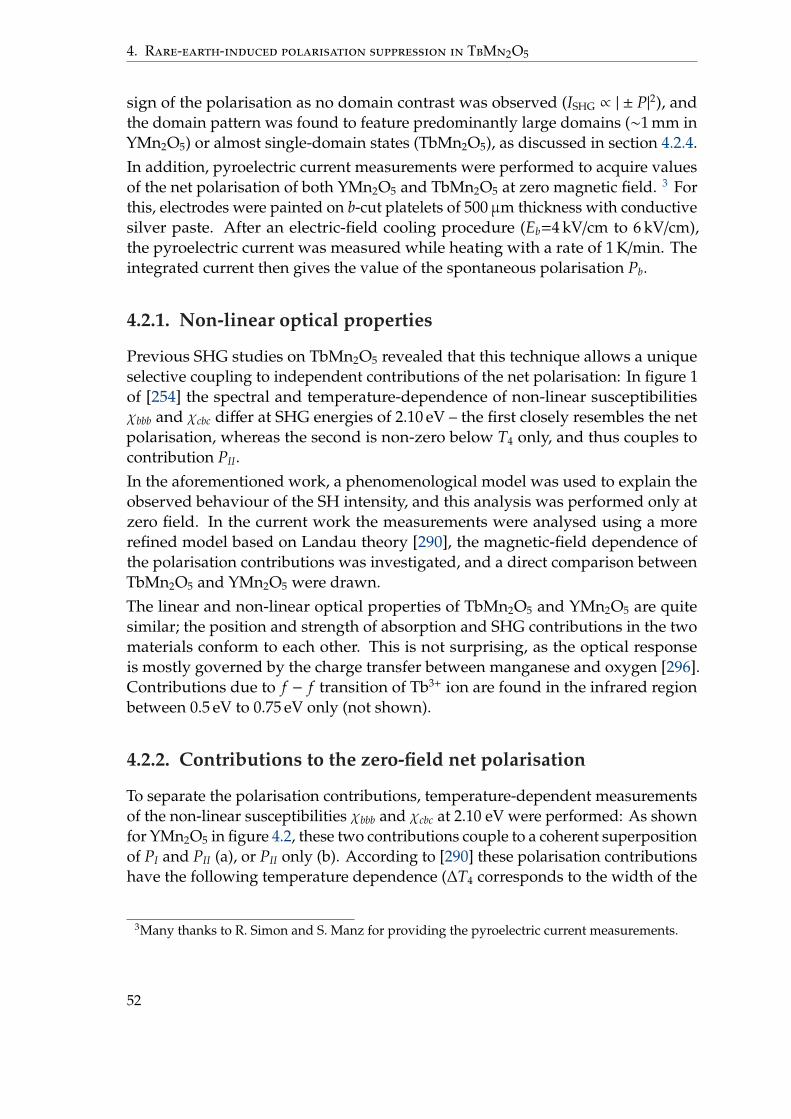
4. Rare-earth-induced polarisation suppression in TbMn2O5
sign of the polarisation as no domain contrast was observed (ISHG ∝ | ± P|2), andthe domain pattern was found to feature predominantly large domains (∼1 mm inYMn2O5) or almost single-domain states (TbMn2O5), as discussed in section 4.2.4.In addition, pyroelectric current measurements were performed to acquire valuesof the net polarisation of both YMn2O5 and TbMn2O5 at zero magnetic field. 3 Forthis, electrodes were painted on b-cut platelets of 500µm thickness with conductivesilver paste. After an electric-field cooling procedure (Eb=4 kV/cm to 6 kV/cm),the pyroelectric current was measured while heating with a rate of 1 K/min. Theintegrated current then gives the value of the spontaneous polarisation Pb.
4.2.1. Non-linear optical properties
Previous SHG studies on TbMn2O5 revealed that this technique allows a uniqueselective coupling to independent contributions of the net polarisation: In figure 1of [254] the spectral and temperature-dependence of non-linear susceptibilitiesχbbb and χcbc differ at SHG energies of 2.10 eV – the first closely resembles the netpolarisation, whereas the second is non-zero below T4 only, and thus couples tocontribution PII.In the aforementioned work, a phenomenological model was used to explain theobserved behaviour of the SH intensity, and this analysis was performed only atzero field. In the current work the measurements were analysed using a morerefined model based on Landau theory [290], the magnetic-field dependence ofthe polarisation contributions was investigated, and a direct comparison betweenTbMn2O5 and YMn2O5 were drawn.The linear and non-linear optical properties of TbMn2O5 and YMn2O5 are quitesimilar; the position and strength of absorption and SHG contributions in the twomaterials conform to each other. This is not surprising, as the optical responseis mostly governed by the charge transfer between manganese and oxygen [296].Contributions due to f − f transition of Tb3+ ion are found in the infrared regionbetween 0.5 eV to 0.75 eV only (not shown).
4.2.2. Contributions to the zero-field net polarisation
To separate the polarisation contributions, temperature-dependent measurementsof the non-linear susceptibilities χbbb and χcbc at 2.10 eV were performed: As shownfor YMn2O5 in figure 4.2, these two contributions couple to a coherent superpositionof PI and PII (a), or PII only (b). According to [290] these polarisation contributionshave the following temperature dependence (∆T4 corresponds to the width of the
3Many thanks to R. Simon and S. Manz for providing the pyroelectric current measurements.
52

4.2. Optical analysis of polarisation contributions
Figure 4.2. Polarization contributions in YMn2O5: (a,b) Temperature dependence ofthe SHG contributions from (a) χbbb and (b) χcbc measured in the same experimentalrun at 2~ω=2.10 eV. (c) Comparison of the sum Pb = PI − PII (as obtained from SHGmeasurements) with the net polarisation obtained by pyroelectric current measurements.The correlation is apparent. Solid lines in (a) to (c) mark Landau theoretical fits.
first-order transition):
P2I (T) =
m2(T3 − T) + (m1 −m2)(T2 − T3) T < T3
m1(T2 − T) T3 < T < T2
0 T > T2
(4.1)
PII(T) =
m′2(T4 − T) + (m′1 −m′2)∆T4 T < T4 − ∆T4
m′1(T4 − T) T4 − ∆T4 < T < T4
0 T > T4
(4.2)
One can obtain proper agreements by fitting the SHG intensities Ibbb(T > T4) ∝ P2I (T)
and Icbc(T) ∝ P2II(T), as shown by green and blue solid lines in figure 4.2, respectively.
Below T4, χbbb is described by a coherent superposition of both contributions (withrelative amplitude and phase A and φ, respectively), shown by the grey line:
Ibbb(T < T4) = |PI − AeiφPII|2 . (4.3)
The sum Pb = PI −PII gives the net polarisation in YMn2O5 obtained by pyroelectriccurrent measurements with the drastically reduced P value below T4, as shown infigure 4.2 (c). Here, the values for the transition temperatures were slightly shifted,4
while the slopes of the fitting functions to the SHG intensities were left unchanged.An analogous analysis can be made for TbMn2O5 as shown in figure 4.3: As in thecase for YMn2O5,χbbb andχcbc at SH energy of 2.08 eV were measured simultaneouslywhile heating. Again, χbbb in (a) behaves similar to the net polarisation (shown in
4Due to heating with the intense laser light the transitions appear at slightly lower temperaturecompared to the literature values or pyroelectric current measurements.
53
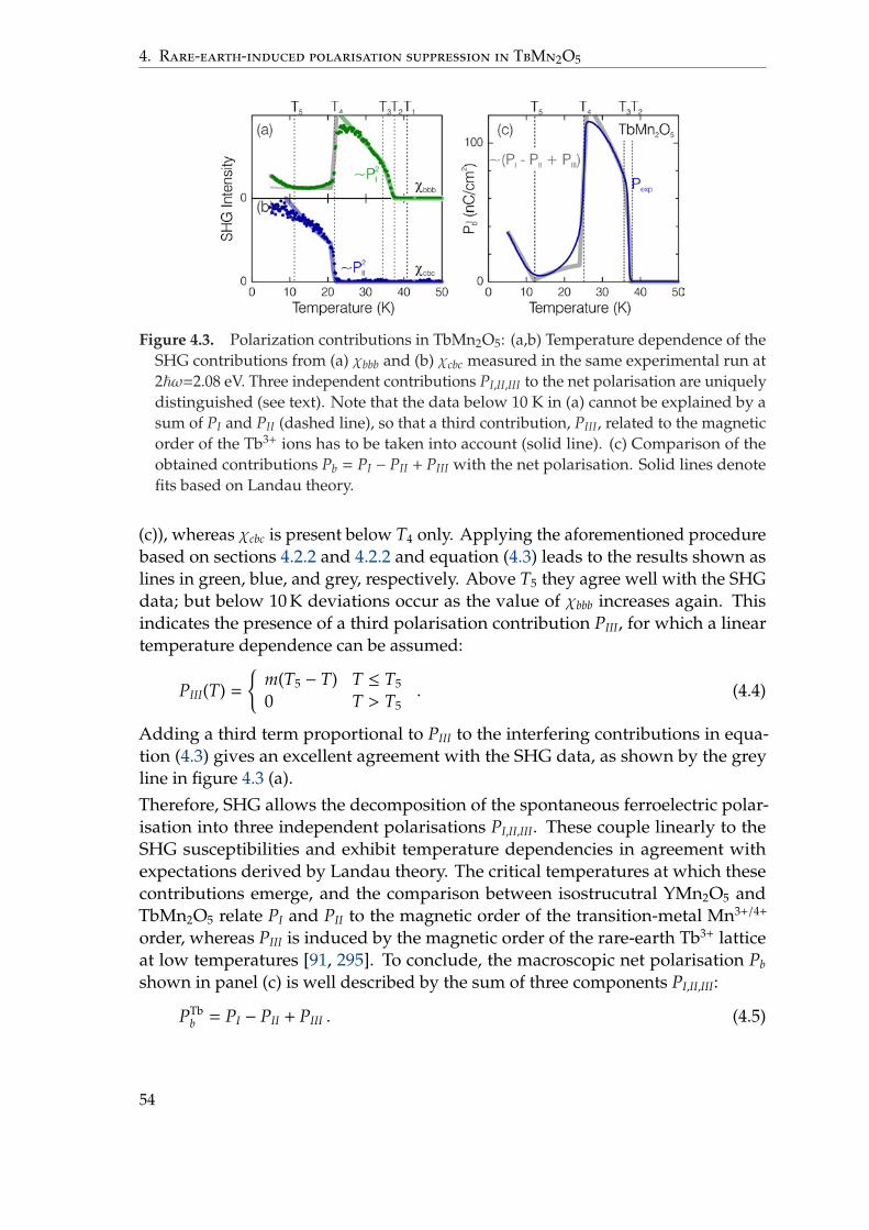
4. Rare-earth-induced polarisation suppression in TbMn2O5
Figure 4.3. Polarization contributions in TbMn2O5: (a,b) Temperature dependence of theSHG contributions from (a) χbbb and (b) χcbc measured in the same experimental run at2~ω=2.08 eV. Three independent contributions PI,II,III to the net polarisation are uniquelydistinguished (see text). Note that the data below 10 K in (a) cannot be explained by asum of PI and PII (dashed line), so that a third contribution, PIII, related to the magneticorder of the Tb3+ ions has to be taken into account (solid line). (c) Comparison of theobtained contributions Pb = PI − PII + PIII with the net polarisation. Solid lines denotefits based on Landau theory.
(c)), whereas χcbc is present below T4 only. Applying the aforementioned procedurebased on sections 4.2.2 and 4.2.2 and equation (4.3) leads to the results shown aslines in green, blue, and grey, respectively. Above T5 they agree well with the SHGdata; but below 10 K deviations occur as the value of χbbb increases again. Thisindicates the presence of a third polarisation contribution PIII, for which a lineartemperature dependence can be assumed:
PIII(T) =
{m(T5 − T) T ≤ T5
0 T > T5. (4.4)
Adding a third term proportional to PIII to the interfering contributions in equa-tion (4.3) gives an excellent agreement with the SHG data, as shown by the greyline in figure 4.3 (a).Therefore, SHG allows the decomposition of the spontaneous ferroelectric polar-isation into three independent polarisations PI,II,III. These couple linearly to theSHG susceptibilities and exhibit temperature dependencies in agreement withexpectations derived by Landau theory. The critical temperatures at which thesecontributions emerge, and the comparison between isostrucutral YMn2O5 andTbMn2O5 relate PI and PII to the magnetic order of the transition-metal Mn3+/4+
order, whereas PIII is induced by the magnetic order of the rare-earth Tb3+ latticeat low temperatures [91, 295]. To conclude, the macroscopic net polarisation Pb
shown in panel (c) is well described by the sum of three components PI,II,III:
PTbb = PI − PII + PIII . (4.5)
54

4.2. Optical analysis of polarisation contributions
Figure 4.4. Magnetic-field dependence of polarisation contributions in YMn2O5. (a)and (b) show the temperature-dependence of χbbb and χcbc (2~ω=2.10 eV) at differentfields µ0Ha, respectively. The magnetic field Ha only stabilizes the low-temperatureincommensurate phase, as indicated by the slight increase of first-order-transitiontemperature T4, whereas the SH intensity remains unaffected. This is also illustratedin panel (c) to (e), which show the magnetic-field dependence of SHG contributions atdifferent temperatures. Solid lines denote constant fits. (f) Two-polarisation model withrobust polarisation contributions PI(T) and PII(T), shown in green and blue. The netpolarisation is indicated in grey.
4.2.3. Magnetic-field dependence of the polarisation
After demonstrating the separation of independent contributions to the net polari-sation by optical SHG, their magnetic-field dependence is investigated. For this,fields µ0Ha up to 7 T are applied along the crystallographic a direction. NeitherYMn2O5 nor TbMn2O5 showed a sign-dependent magnetoelectric effect.The situation is quite simple in YMn2O5, as shown in figure 4.4: Apart from aslight increase in the first-order transition temperature T4, the temperature- andmagnetic-field dependence of χbbb and χcbc remains constant for fields up to 7 T, asshown in panels (a) to (e). As a consequence, the polarisation contributions PI andPII, and the net polarisation as shown in figure 4.4 remain largely unaffected by themagnetic field, supporting claims of the robustness of the Mn3+/4+ order [297, 298].At first glance the situation in TbMn2O5 is similar to that of YMn2O5: Figure 4.5(a,b) shows the temperature-dependence of χbbb and χcbc in different magnetic fields.Again, a stabilization of the low-temperature phase is observed in agreement with[91, 298], which is more pronounced than in YMn2O5. Also the contributionscoupling to PI and PII remain unaffected by the applied field, as clearly seen bytheir constant behaviour in field-sweeps given in panels (c) and (e).At low temperatures, however, χbbb shows a very remarkable dependence uponapplication of a magnetic field, as shown in figure 4.5 (a) and (d): The high intensityat zero field is largely suppressed even by small values of µ0Ha, and has a minimumnear 3 T. As both PI and PII are field-independent, this change must be attributed
55

4. Rare-earth-induced polarisation suppression in TbMn2O5
Figure 4.5. Magnetic-field dependence of the polarisation contributions in TbMn2O5.Panels (a) and (b) show the temperature-dependence of χbbb and χcbc (2~ω=2.08 eV) atdifferent magnetic fields µ0Ha, respectively. At non-zero field the low-temperature signalof χbbb is suppressed, while the shift of the first-order transition to higher values is morepronounced than in YMn2O5. (c-e) Magnetic-field dependence of SHG contributionsat different temperatures. Only at low temperatures the contribution χbbb coupledto PIII shows a pronounced magnetic-field dependence linked to the magnetization,while SH contributions coupling to PI and PII remain constant. Solid lines denotes (c,e)linear fits or (d) a fit based on equation (4.6). (f) Proposed three-polarisation model toexplain the complicated temperature- and magnetic field dependence of the ferroelectricnet-polarisation PTb
b = PI − PII + PIII as observed in [91].
to the rare-earth induced polarisation contribution PIII. Furthermore, the field-dependence of PIII(T,Ha) can be related to the sample magnetization by the simplequadratic relationship
PIII(Ha,T) = PIII(0,T) − βM2a(Ha,T) , (4.6)
with the assumption that the magnetization is given by the alignment of the largerare-earth moments described by a Brillouin function Ma ∝ BJ(T,Ha) with J = 6and gJ = 1.5 for Tb3+ (configuration 4 f 8) [91]. As a result, the contribution χbbb
rapidly decreases with increasing field, and shows a minimum near 3 T wherethe magnetization saturates and PIII changes its sign; which is underlined by thegood agreement between SHG data and the fit function in figure 4.5 (d). Sincethe magnetic moments closely follow the field in a paramagnetic fashion, nohysteresis is observed. The sign-independence of the polarisation suppression isalso suggested by the squared dependence of the induced magnetisation.In comparison with integrated methods like pyroelectric current measurementswhich measure the net polarisation only, here the behaviour of the three ferroelectriccontributions can be separated unambiguously. Their temperature- and magnetic-field dependence culminates in the three-polarisation model shown in figure 4.5 (f):Robust manganese magnetism induces the largely field-independent contributionsPI and PII, whereas the pronounced magnetoelectric effect is linked to the low-
56

4.2. Optical analysis of polarisation contributions
Figure 4.6. Domains in TbMn2O5. Imaging with χbbb ∝ Pb at 2.08 eV at 5 K. Applicationof magnetic fields leads to additional needle-like structures along the polar b direction.The overall ferroelectric domain pattern stays unchanged by the magnetic field, however.The scale bar measures 500µm.
temperature, rare-earth induced polarisation PIII and its suppression as the appliedfield aligns the large Tb moments parallel to the field direction.
4.2.4. Ferroelectric domains
To verify that the magnetoelectric coupling is a coherent process not involvingdomain wall movement, SHG imaging experiments were also employed, as shownin figures 4.6 and 4.7.5
Zero-field domain patterns Usually, TbMn2O5 forms an almost single-domainstate like the one shown in figure 4.6 (a). These domains are very stable once cooledbelow T3, even when repeatedly cycling across the first-order phase transition atT4. In contrast, YMn2O5 shows a multi-domain state, and pronounced hysteresisat T4: Figure 4.7 (a) and (b) show the domain re-arrangement for a cooling cycle,while the comparison of (b) and (d) gives the changes upon heating across thefirst-order transition. The pattern in figure 4.7 (d) can be due to the interference ofSHG contributions of domains staggered along the optical path.Overall, the typical domain size is several hundredµm, which is orders of magnitudelarger than for conventional ferroelectric materials. The shapes of the domains arequite random, but the domain walls show a slight preference to align along thepolar b direction. Both materials show a pronounced domain memory effect due topinning, and only heating the sample at least 50 K above the Néel temperature T1
leads to changes the domain pattern.In both YMn2O5 and TbMn2O5 imaging with χbbb and χcbc leads to the same results,indicating that contributions PI and PII are not induced by different ferroelectricdomains (not shown). Furthermore, the application of a magnetic field does notchange the distribution of the polar domains, shown by comparing figure 4.6 (a)
5The SHG images show interference fringes due to the long coherence length of the ns laser pulseand the thin sample. In figures 4.6 and 4.7 these brightness variations are slightly reduced byoverlaying the image with an inverted, smoothed version of itself.
57

4. Rare-earth-induced polarisation suppression in TbMn2O5
Figure 4.7. Ferroelectric domains in YMn2O5. Imaging with χbbb ∝ Pb at 2.10 eV. Thescale bar measures 500µm. In contrast to TbMn2O5, the domain pattern in YMn2O5
changes when cooling or heating across the first-order transition at T4=19 K.
and (b) or figure 4.7 (b) and (c) for example. This indicates that indeed PI, PII, andPIII are induced due to microscopic interactions in the same domain. Therefore themagnetic-field induced polarisation suppression in TbMn2O5 should not be called“reversal” or “switching” as in [91], as these terms are associated to the changefrom ±P to ∓P involving hysteretic domain formation and motion. Here, onlythe balance of different contributions to the net polarisation is changed with themagnetic field.Needle-like patterns in TbMn2O5 The situation is more complicated in TbMn2O5
where, in magnetic fields, additional needle-like stripes along b are observed: At5 K they appear for µ0Ha above 3 T, and multiply in number for higher fields as seenin figure 4.6 (b) and (c). Once formed, they persist when removing or reversingthe magnetic field at low temperatures (figure 4.6 (c) and (d)). They are moremobile at higher temperatures and disappear when heated above T4. Therefore onemight conclude that the needle-like domains are related to the low-temperatureincommensurate phase and the occurrence of the magnetization of the Tb3+ sub-lattice; however, they do not simply trace M domains as the sample is expected tobe uniformly magnetized at high field (as indicated by the coherent signal reductiontracing Pb).No conclusions can be made about origin and actual size of these needle-likestructures, but it is important to emphasize that they do not contribute to theobserved magnetoelectric effect and three-polarisation model as presented infigure 4.5 (f): Firstly, the largest field-dependent response of both the SHG signaland Pb is observed below 3 T, where the stripes initially do not occur. Secondly,the presence of the stripes does not affect the behaviour of field- or temperature-dependent measurements – in the former case they mostly stay unchanged, inthe latter they disappear upon heating. Therefore, these patterns are not directlyrelated to the presence of PIII, and its field-dependent behaviour.
58

4.3. Magnetoelectric coupling in RMn2O5
4.3. Magnetoelectric coupling in RMn2O5
As shown in the previous sections, SHG experiments can disentangle independentcontributions to the ferroelectric net polarisation in RMn2O5 and investigate theirresponse to an applied magnetic field. Furthermore, the coupling of the light fieldsto the electronic structure reveals clues about the microscopic interactions leadingto multiferroic and magnetoelectric behaviour in this class of materials. Theseobservations and conclusions are discussed in the following section.
4.3.1. Transition-metal-induced multiferroicity
The two polarisation contributions PI and PII, observed in both TbMn2O5 andYMn2O5, are linked to the magnetic order of 3d transition metal Mn3+/4+ ions,as indicated by the close relationship between ferroelectric and magnetic phasetransitions in figure 4.1. PI and PII maintain an anti-parallel orientation, leading toa sudden drop of the net polarisation Pb = PI − PII with the emergence of PII belowthe first-order transition at T4. This behaviour was predicted by phenomenologicalmodels and Landau theory previously [91, 290], but the independent observationof both contributions via SHG unambiguously confirms their opposite sign.The spin order of the Mn ions and the related polarisation contributions PI and PII
is affected neither by magnetic fields ±µ0Ha up to 7 T nor the rare-earth magneticorder in TbMn2O5. This is clearly demonstrated by the measurements in figures 4.4and 4.5, and has also been shown by neutron scattering experiments [298]. Theapplied field has some effect on the magnetic structure, however, as in both YMn2O5
and TbMn2O5 as well as iso-structural DyMn2O5 [299] and ErMn2O5 [164] thelow-temperature incommensurate phase, and thus the presence of PII, is stabilized.On that note, the presence of at least two contributions PI and PII seems to bea uniting feature in the family of multiferroic RMn2O5: The comparison of theferroelectric properties, e.g. shown in [300, fig. 2],6 reveals similar transitiontemperatures, as well as comparable magnitudes of the spontaneous polarisation[300–304]. These similarities further underline the remarkable stability of the 3dspin order and its role for the ferroelectric properties in the RMn2O5 series.The microscopic mechanism inducing the net polarisation is not yet clear. Manyresults point to symmetric exchange striction between collinear Mn moments[140, 141, 305] as the predominant source. Additionally, contributions due toanti-symmetric exchange are proposed [303, 306] as well as local dipoles due top-d hybridisation [154, 296, 307]. Also, those combinations of all contributions arediscussed [300, 308].
6The comparison in [300] would be more striking if newer and more accurate pyroelectric currentmeasurements for the ferroelectric polarisation had been included.
59

4. Rare-earth-induced polarisation suppression in TbMn2O5
4.3.2. Rare-earth-induced magnetoelectric coupling
In contrast to the two previously discussed ferroelectric contributions, the thirdpolarisation PIII was observed in TbMn2O5 only. Here, it was shown that thiscontribution emerges at low temperatures only, and is solely responsible for themagnetoelectric coupling observed in TbMn2O5. Due to the close relationshipbetween magnetisation, rare-earth moment, and PIII, the 4 f spin order seems to beof integral importance in explaining the magnetoelectric properties of this material.Zero-field polarisation For the emergence of PIII in zero field it helps to understandthe evolution of the rare-earth magnetic order upon cooling: A portion of theTb3+ moments already order below the Néel temperature T1, as they are spin-polarized by the ordered Mn3+/4+ spins [293, 309, 310]. On the other hand, isotropicTb3+-Tb3+ exchange can induce long-range order below T5 ≈10 K, and indeedantiferromagnetic order of the rare-earth ions with the same incommensurate wavevector q as the Mn order is observed [309, 311, 312]. This phase transition isaccompanied by a small characteristic hump in the dielectric function εb [312, 313],supporting the emergence of an additional polarisation contribution PIII.The assumption of the linear increase of PIII(T) upon cooling presented in fig-ure 4.3 (c) is supported by the Landau theoretical predictions: The irreduciblerepresentation of the Tb order and the subsequent symmetry-allowed couplingsfor PIII are the same as for PII [290]. A linear increase of PIII(T) with lower T alsois proportional to the increase of the ordered rare-earth moment and thus themagnitude of the antiferromagnetic order parameter below 10 K [309–312].Field-dependent behaviour As shown in figure 4.5 (d) and equation (4.6), the field-dependent response of PIII(Ha) is directly correlated to the induced magnetisationMa(Ha): As the magnetisation increases proportional to the applied field, thepolarisation contribution PIII decreases quadratically with Ma. For fields of around3 T the magnetisation saturates, and PIII changes sign. This behaviour points toa strong competition between antiferromagnetic Tb order on the one hand, andalignment of the large rare-earth moments on the other hand, as independent, butclosely interwoven, mechanisms contributing to the magnetoelectric response.At zero field, only the antiferromagnetic order of the rare-earth sub-lattice con-tributes to PIII = PAFM
III . Due to the large 4 f moment, a small field Ha induces amagnetisation along the field direction, which in turn diminishes the antiferromag-netic arrangement of the Tb moments [91, 295, 314]. Consequently, the magnitudeof the ferroelectric contribution PAFM
III is reduced:
PAFMIII (T,Ha) = PAFM
III (T, 0) − β1(Ma)M2a(T,Ha) , (4.7)
The coupling constant β1(Ma) is determined by the condition
limHa→∞
PAFMIII (T,Ha) = 0 , (4.8)
60

4.3. Magnetoelectric coupling in RMn2O5
so that this contribution vanishes completely once the 4 f moments are fully alignedwith the magnetic field.Additionally, a quadratic magnetoelectric effect PPM
III (T,Ha), induced by the param-agnetic alignment of the rare-earth moments, contributes to the field-dependentresponse. This effect leads to the upturn of the SHG intensity for high fields shownin figure 4.5 (d) as the sign of PIII = PAFM
III − PPMIII reverses [295]. Its temperature- and
field-dependence is given by
PPMIII (T,Ha) = β2M2
a(T,Ha) . (4.9)
Here, β2 parametrizes the quadratic coupling term [295, 315]. This contributionalso persists at temperatures higher than T5 [91, 316], which once more emphasizesits relation to the induced magnetization instead to the long-range Tb order.The overall field-response of the polarisation contribution PIII therefore is given bythe following sum:
PIII(T,Ha) = PAFMIII (T,Ha) − PPM
III (T,Ha) (4.10)= PAFM
III (T, 0) +[−β1(Ma) + β2
]M2
a(T,Ha) . (4.11)
The antiparallel configuration and different magnitude of PAFMIII (T,Ha) and PPM
III (T,Ha)leads to the sign change of PIII, and consequently of Pb, at high magnetic fields [91].Microscopic mechanisms Below T5 the Tb3+ moments are aligned collinearly[293], which could lead to a finite polarisation due to exchange striction. Anotherpossibility to induce a ferroelectric contribution would be the emergence of localdipoles due to p- f hybridisation, as described in section 2.2.2.Further insight to the microscopic origin of PIII is given by the optical non-linearproperties: In both YMn2O5 and TbMn2O5 the SHG signal is sensitive to thepolarisation contributions PI,II. These excitations couple to Mn→ O charge-transferexcitations [254, 296], and thus are sensitive to the transition-metal magnetism.In contrast, the SHG signal proportional to the low-temperature polarisation inTbMn2O5 does not couple directly to the rare-earth order, as no Tb3+ excitations arepresent in the studied spectral range. Therefore, an indirect optical coupling to the4 f moments must be present via induced effects on either the Mn or O sites.As the polarisation contributions PI and PII are independent of the applied field theMn3+/4+ ions are largely unaffected by the Tb order [298], which leaves oxygen asthe main ingredient of the microscopic magnetoelectric coupling.Recent publications indeed show the important role of oxygen for the multiferroicproperties of RMn2O5 materials [154, 311, 317]. Furthermore, the oxygen bondpolarisation was shown to depend on the rare earth order [307, 318]. Due to thesusceptibility of the large 4 f 8 moment (|µ| ≈ 8.2µB [91, 295]) to magnetic fields,
61

4. Rare-earth-induced polarisation suppression in TbMn2O5
the oxygen-rare-earth hybridisation therefore offers the possibility of pronouncedmagnetoelectric effects as observed in multiferroic TbMn2O5.7
4.4. Summary
In conclusion, two (three) independent contributions to the spontaneous polarisa-tion in multiferroic YMn2O5 (TbMn2O5) were separated using non-linear opticalsecond harmonic generation. Their respective temperature and field dependencewere investigated, and related to a Landau-theoretical model.Polarization contributions PI and PII induced by the complex order of Mn3+/4+
moments were found in both materials. Their sum Pb = PI −PII explains the specifictemperature-dependence of the net polarisation Pb with a sudden drop at themagnetic phase transition where also PII emerges. Both PI and PII were shown tobe robust under magnetic fields ±µ0Ha up to 7 T. These robust contributions seemto be a general feature for the multiferroic properties of RMn2O5 materials.In TbMn2O5 an additional contribution PIII explained both the recovery of Pb atlow temperatures and the pronounced magnetoelectric coupling induced by thelong-range rare-earth order and – due to the large 4 f moment – readily influencedby an applied magnetic field. The optical properties indicated that the interactionbetween rare-earth order and hybridisation with the surrounding oxygen ionscould be the main ingredient to this pronounced magnetoelectric coupling.
7Many thanks to P. Tolédano and R.V. Pisarev for fruitful discussions about the origin of PIII.
62
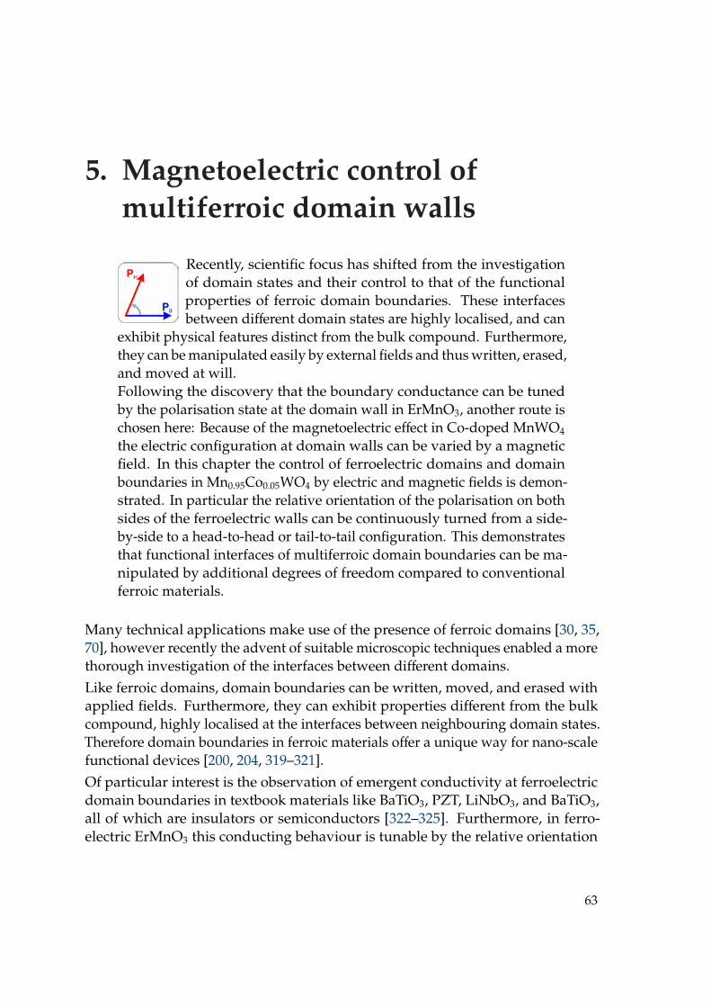
5. Magnetoelectric control ofmultiferroic domain walls
Recently, scientific focus has shifted from the investigationof domain states and their control to that of the functionalproperties of ferroic domain boundaries. These interfacesbetween different domain states are highly localised, and can
exhibit physical features distinct from the bulk compound. Furthermore,they can be manipulated easily by external fields and thus written, erased,and moved at will.Following the discovery that the boundary conductance can be tunedby the polarisation state at the domain wall in ErMnO3, another route ischosen here: Because of the magnetoelectric effect in Co-doped MnWO4
the electric configuration at domain walls can be varied by a magneticfield. In this chapter the control of ferroelectric domains and domainboundaries in Mn0.95Co0.05WO4 by electric and magnetic fields is demon-strated. In particular the relative orientation of the polarisation on bothsides of the ferroelectric walls can be continuously turned from a side-by-side to a head-to-head or tail-to-tail configuration. This demonstratesthat functional interfaces of multiferroic domain boundaries can be ma-nipulated by additional degrees of freedom compared to conventionalferroic materials.
Many technical applications make use of the presence of ferroic domains [30, 35,70], however recently the advent of suitable microscopic techniques enabled a morethorough investigation of the interfaces between different domains.Like ferroic domains, domain boundaries can be written, moved, and erased withapplied fields. Furthermore, they can exhibit properties different from the bulkcompound, highly localised at the interfaces between neighbouring domain states.Therefore domain boundaries in ferroic materials offer a unique way for nano-scalefunctional devices [200, 204, 319–321].Of particular interest is the observation of emergent conductivity at ferroelectricdomain boundaries in textbook materials like BaTiO3, PZT, LiNbO3, and BaTiO3,all of which are insulators or semiconductors [322–325]. Furthermore, in ferro-electric ErMnO3 this conducting behaviour is tunable by the relative orientation
63

5. Magnetoelectric control of multiferroic domain walls
of the polarisation at the wall: Due to charge accumulation and subsequent elec-tronic screening, head-to-head or tail-to-tail boundaries show a distinctly differentconducting behaviour to charge-neutral side-by-side domain walls [326].In hexagonal RMnO3 the curved domain walls are a consequence of the improperferroelectric order and topologically protected due to their structural origin [327,328]. In contrast, magnetoelectric materials offer another route to influence thepolarisation state at the ferroelectric domain boundaries: In several spin-spiralmultiferroic materials like orthorhombic RMnO3 (R = Tb, Dy), MnWO4, LiCuVO4,or RMn2O5 (R = Tm, Yb) a magnetic-field-induced polarisation flop was observed[90, 163, 178, 180, 181, 329]: As discussed in 2.3.1 the magnetic structure and theferroelectric polarisation suddenly re-orient above a critical field.An even more precise way to control the polarisation state is found in Co-dopedMnWO4, which shows a continuous rotation of the net polarisation with appliedmagnetic field [184]. Here it is shown that the position of domain boundaries inMn0.95Co0.05WO4 does not change upon the magnetic-field induced polarisationrotation. As a consequence, the ferroelectric state at the domain boundary canbe continuously and reversibly tuned by an applied magnetic field. Thus, incombination with an electric field, both domain wall position and state can be fullycontrolled.In the following sections, the magnetic, electric, and optical properties of Co-dopedMnWO4 are discussed first. Then the exclusive coupling of second harmonicsignals to the ferroelectric polarisation contributions is shown. This can be used tovisualise the electric- and magnetic-field control of the domain boundary positionand its polarisation state. The experimental results will be followed by a briefdiscussion about the microscopic structure of multiferroic domain boundaries andimplications for possible functional behaviour.
5.1. Multiferroic tungstates
Isomorphous transition-metal tungstates Me2+WO4 with Me = Mg, Mn, Fe, Co,Ni, Zn, and Cd crystallise in the wolframite structure shown in figure 5.1 (a) [331].This crystallographic structure is based on a hexagonal close-packaging of oxygenions. Cations fill half of the octahedral interstitial sites and the edge-sharingoctahedra surrounding the transition-metal ions Me2+ form zigzag ribbons alongthe c direction [332]. The space group is P2/c1′ with two-fold symmetry axis along b,and the monoclinic angle β only deviating slightly from 90◦ (typically less than 1◦).Prominent in the series of tungstates is MnWO4 which shows multiferroic behaviourbetween 7 K to 12 K. The spontaneous polarisation P||b up to 40 nC/cm2 is inducedby cycloidal spin-spiral order [130, 333], as schematically shown in figure 5.1 (b).For magnetic field H||b above 10.5 T, a spin-flop transition with a 90◦ reorientation
64

5.1. Multiferroic tungstates
Figure 5.1. Structural and magnetic properties of Mn0.95Co0.05WO4. (a) Crystallographicwolframite structure, with Me2+O6 octahedra (Me = Mn, Co) forming edge-sharingzigzag ribbons along c [330]. (b) Magnetic structure in the multiferroic phase. The spiralpropagates along q = (−0.25+δa, 0.5, 0.5−δc); while the spins rotate within the easy plane℘ containing the polar b direction. ℘ is inclined from the ac plane. Adapted from [110].(c) Relative magnitude and direction of the net polarisation at 5 K [184]: A moderatefield H||b rotates the initial polarisation P||b towards the a direction due to a rotation ofspin-spiral plane ℘.
of the polarisation towards the a direction is observed in MnWO4 [178]. Thismagnetic transition is the result of a competition between exchange interactionsand the magneto-crystalline anisotropy, as discussed in section 2.3.1.Other wolframites show different magnetic behaviour, which is largely determinedby the properties of the respective transition-metal ions Me2+. Therefore, dop-ing MnWO4 with magnetic and non-magnetic ions can lead to changes in themultiferroic properties of the base material [139, 334, 335].Especially interesting magnetic properties are achieved in Co-doped MnWO4 asthe single-ion anisotropy of Mn2+ (d5) and Co2+ (d7) are decidedly different: Whilethe easy axis of MnWO4 lies at an angle of approximately 34◦ towards a in the acplane [332, 336, 337], that of CoWO4 is at 133◦ [338]. As consequence, Co dopingwill strongly affect the multiferroic properties of MnWO4 and its behaviour underapplied magnetic fields, as shown in various studies [110, 184, 334, 335, 339–345].In this chapter, MnWO4 with 5% Co-doping is investigated: In this material it ispossible to continuously rotate the ferroelectric polarisation with a magnetic field[184]. The light doping induces only small changes in the crystal structure, and theferroelectric transition temperature TC ≈12 K and the magnetic propagation vectorq = (−0.25 + δa, 0.5, 0.5 − δc) remain mostly unaffected [110].In contrast, the multiferroic phase is stabilised down to low temperatures, and thespin-spiral plane ℘ determined by the magnetic anisotropy is less inclined towardsthe a axis as for un-doped MnWO4 [110, 334]. At zero field, the polarisation isaligned mostly along b, but with applied magnetic field Hb the net polarisation
65

5. Magnetoelectric control of multiferroic domain walls
gradually rotates towards the a direction, as shown in figure 5.1 (c) [184].The polarisation control by a magnetic field in Mn0.95Co0.05WO4 offers a greatopportunity to investigate the behaviour of multiferroic domains and domainboundaries under the effect of gradually changing the configuration of the domainboundary from side-to-side to tail-to-tail or head-to-head configuration.
5.2. Experimental details
Here, optical second harmonic generation is used to detect and image domains ofpolarisation contributions Pb and Pa, and determine their behaviour under appliedelectric and magnetic fields. This section briefly describes the sample preparationand the experimental setup.Sample preparation Large single-crystal samples (up to 50 mm3) of Mn0.95Co0.05WO4
grown by the floating-zone method were provided by Jack Kao-Cheng Liang andBernd Lorenz from the University of Houston, USA. Three platelets oriented alongthe crystallographic a, b and c direction were lapped to a thickness of 100µm andpolished with silica slurry in preparation for optical transmission experiments. Asthe wolframite structure shows a cleavage along the ac plane, the b-cut sampleyielded very flat surfaces. The preparation of the a-cut sample was also satisfactory,whereas the c-cut gave only mediocre surface flatness. Fortunately, these defectsdid not hamper later results.Linear optical properties The polarised absorption spectra of Mn0.95Co0.05WO4
were measured at room temperature as described in section 3.5.1 and compared tocorresponding spectra of pure MnWO4.SHG experiment The non-linear optical experiments were performed in transmis-sion geometry. A tunable fs laser was used as light source, and the non-linearresponse was detected either with a liquid-nitrogen cooled CCD camera or with aphotomultiplier for integrated measurements. The sample was located in a magnetcryostat with magnetic fields ±µ0Hb up to 7 T in Voigt configuration (Hb ⊥ (k||c)).Using a special sample holder in-plane electric fields up to approximately 5 kV/cmcould be applied along the polar a or b directions.
5.3. Linear optical properties of Mn0.95Co0.05WO4
The polarised absorption spectra of Mn0.95Co0.05WO4 are shown in figure 5.2:As expected by the monoclinic symmetry, the material shows a pronouncedpleochroism, and the absorption ellipsoid was slightly inclined from the a and caxes [346].
66

5.4. Distinction of ferroelectric contributions by SHG
Figure 5.2. Linear absorption coefficients αi(ω) of Mn0.95Co0.05WO4 at room temperature.On the bottom the determined positions and widths of crystal-field transitions aremarked. The colours illustrate the optical pleochroism of the material. Comparison withpure MnWO4 reveals that the observed absorption peaks and green colour is most likelycaused by crystal-field transitions of Co2+ ions. The inset shows the orientation of theabsorption ellipsoid in the ac plane at 2.15 eV. The offset angle is approximately 10◦, butits sign towards the monoclinic a direction could not be determined.
In the case of pure MnWO4 only weak absorption is observed, with the lowest-lyingcrystal-field excitation at 2.20 eV [252, 347]. In contrast, dd excitations of Co2+
ions (configuration d7) are only parity-forbidden, but not spin-forbidden, as inthe case for Mn2+ ions (d5). Therefore, the absorption is expected to be strongerin Mn0.95Co0.05WO4: While thin platelets of MnWO4which appear light orange intransmission, the Co-doping lends to a dark green colour.Furthermore, additional excitations due to Co2+ ions are observed centred at 0.75 eV,1.48 eV, and around 2.17 eV. The latter is a combination of Mn and Co dd transitions,but its splitting to three peaks is typical for Co2+ [106].Further d-d transitions are known to exist above 2.5 eV [252] where the opticalresponse is dominated by O 2p→Mn 3d charge-transfer [347–349].
5.4. Distinction of ferroelectric contributions by SHG
To image the ferroelectric domain population and their temperature- and field-dependence of both Pb and Pa, SHG signals coupling to both polarisation directionsare required. SHG signals related to Pb in undoped MnWO4 were previouslyinvestigated and were used to image the ferroelectric domains topography, andthe electric-field switching process [255, 349–353]. From these previous results itwas found that around 2.15 eV a pronounced SHG signal coupling to Pb [252, 354],greatly enhanced by optical phase matching, is present (see appendix B).Therefore, the search for SHG contributions coupling to polarisations Pb and Pa in
67

5. Magnetoelectric control of multiferroic domain walls
Figure 5.3. Comparison of SHG contributions ∝ Pb (in blue) and ∝ Pa (in red). (a) SHGspectra of χbaa and χabb at different magnetic fields. (b) Temperature dependence ofχbbb and χabb compared to the Pb and Pa contributions at 5 T. χbaa and χbbb show thesame coupling to Pb (not shown). (c) Magnetic-field dependence of SHG contributionsscaled to polarisation values, reflecting the magnetic-field induced 90◦-rotation of the netpolarisation. Polarisation values in (b) extracted from [184], those in (c) were providedby B. Lorenz, University of Houston.
Mn0.95Co0.05WO4 was focussed in the SHG energy range of 1.7 eV to 2.2 eV, and ona c-cut sample with an in-plane configuration of both polar directions.Unsurprisingly, a large signal χbaa ∝ Pb around 2~ω=2.1 eV like in undoped MnWO4
was also found in Mn0.95Co0.05WO4. The SHG contribution χabb ∝ Pa centred at2.2 eV is at least two orders of magnitude weaker – in contrast to the relationbetween Pb and Pa, with the latter being clearly dominant at higher temperaturesand magnetic fields. The agreement with symmetry selection rules and the distinctspectral dependence confirm that indeed independent contribution were found, ascan be seen in figure 5.3 (a).The temperature- and magnetic-field-dependence of both χbaa and χabb furtherconfirm the unique coupling to polarisation contribution Pb and Pa, respectively,as shown in figure 5.3 (b) and (c): Here the magnitude of χ ∝
√ISHG is compared
with the polarisation values obtained by pyroelectric and magnetoelectric currentmeasurements, showing a good agreement. Therefore, it is possible with opticalSHG to couple to independent polarisation contributions and to use those signalsto image the ferroelectric domain pattern, as explained in the next section.
5.4.1. Other spectral contributions
Additional to the mentioned signals used for ferroelectric domain imaging, othernon-liner contributions were found in Mn0.95Co0.05WO4.In the energy range 1.8 eV to 2.2 eV an SHG signal χbbb ∝ Pb was found. It showedan oscillating spectral dependence, and was the same order of magnitude as χabb.While integrated measurements show a good agreement with the temperature- and
68

5.5. Imaging of ferroelectric domains with SHG
magnetic-field-dependent behaviour of Pb, the images proved to be speckled anddid not reproduce the domain images taken with other SHG contributions. This isprobably due to the different absorption properties.No SHG response was found above 2.2 eV. However, at 2.67 eV a strong three-photon fluorescence coupled to the spin-forbidden 2T2 →
4 T2 transition of the Mn2+
ion was found. In previous studies at this energy a SHG response coupling to Pb
was observed [252, 255, 351]. This indicates that the use of femtosecond insteadof nanosecond laser pulses might enable additional non-linear optical excitations[214].
5.5. Imaging of ferroelectric domains with SHG
In the following section the results of SHG imaging of ferroelectric domains areexplained, starting with the proof of conformity of Pb and Pa domains. Thepeculiarities of zero-field cooled domain patterns are discussed, and the control ofthe ferroelectric domains and domain boundary states with applied electric andmagnetic fields is demonstrated.
5.5.1. Direct correspondence of Pb and Pa domains
As indicated by a semi-phenomenological model, the emergence of Pa withincreasing magnetic field is related to the rotation of the spin-spiral plane inMn0.95Co0.05WO4 [110, 334]. Consequently, the Pb and Pa domains are expected tocoincide, rather than showing separate spatial distributions.This assumption is confirmed, by the single-domain patterns after electric-field-cooling cycles: Figure 5.4 (a,b) shows spatially resolved images of χbaa ∝ Pb andχabb ∝ Pa after electric-field cooling with Ea in applied magnetic field µ0Hb =6 T.At higher field the polarisation contribution Pa is dominant and field-cooling willlead to a ferroelectric single-domain state. Imaging with χbaa ∝ Pb shows uniformbrightness, and thus a single-domain state, too.A similar result is obtained after electric-field cooling with applied Eb at fieldsbelow 2 T, again leading to a single-domain state in both Pb and Pa (not shown).As electric-field poling either with Ea or Eb leads to simultaneous single-domainstates in both Pa and Pb, imaging with χbaa and χabb gives redundant information,and thereafter the large signal of χbaa can be used to image the ferroelectric domains.
69

5. Magnetoelectric control of multiferroic domain walls
Figure 5.4. Ferroelectric domains in Mn0.95Co0.05WO4: (a,b) Single-domain states obtainedafter electric-field cooling with Ea at 6 T, as indicated by the uniform brightness. That bothPa and Pb appear in the same domain state proves their common origin. (c) As-growndomain pattern after zero-field cooling. Most of the domain boundaries align parallel tothe polar b direction, thus favouring neutral side-by-side domain walls. (d) Same stateas in (c), but imaged with contribution χabb ∝ Pa. The weak signal shows a stripe-likepattern possibly due to depth interference of SHG contributions from different domains.
5.5.2. As-grown domain patterns
As explained in the previous section, ferroelectric Pb and Pa domains coincide as theyare induced by the same microscopic spin spiral structure. The corresponding SHGimages as shown in figure 5.4 (c,d), however, do not match: The pattern observedfor χabb images in figure 5.4 (d) shows stripes aligned along the a direction withaverage distances of 150µm along b and typical lengths of 600µm along a. Theyare clearly of magnetic origin, and change distribution after a heating-and-coolingcycle above TC. For higher magnetic fields they seem to disappear as the SHGsignal of χabb increases, but the pattern re-appears if the magnetic field is removed.The observation of speckled patterns fields implies that the spatial distributionof SHG signal is a consequence of depth interference and not due to the domaindistribution of the net polarisation P.In contrast, χbaa gives clear SHG images of the ferrroelectric domain distribution,e.g. in figure 5.4 (c): The position of the domain boundaries are marked by blacklines, while the domains appear with equal brightness. After zero-field cooling thedomain size varies greatly between large areas of 0.2 mm2 to 1 mm2 and speckledpatterns, which indicate domain sizes below the optical resolution.After zero-field cooling, the domain boundaries show a slight preference to alignalong the polar b direction. Boundaries along a are also readily stabilised, leading tothe conclusion that charge accumulation and electrostatic repulsion at ferroelectrichead-to-head or tail-to-tail walls does not dominate the domain topography inMn0.95Co0.05WO4.Like in other magnetic and multiferroic properties the domain pattern dependson the thermal history of the sample, with strong dependence upon cooling rateacross TC and a pronounced memory effect.
70

5.5. Imaging of ferroelectric domains with SHG
Figure 5.5. Ferroelectric domain switching in Mn0.95Co0.05WO4. (a) Single-domain stateafter electric-field cooling in zero magnetic field. The scale bar measures 250µm. (b)-(e)Subsequence growth of opposite ferroelectric domain in reversed constant electric field.(f) Final two-domain state with preferred side-by-side domain wall configuration.
5.5.3. Electric-field control of ferroelectric domains
To demonstrate the magnetic-field control of the polarisation configuration atthe ferroelectric domain wall, a two-domain state was prepared: As shown infigure 5.5 (a) a single-domain state was obtained by electric-field cooling withEb=3.5 kV/cm and −0.5 K/min at zero magnetic field. At suitably high reversedfield (−4.9 kV/cm at circa 7.5 K), first a domain of opposite polarity nucleated in thetop of the sample and then grew in the constant driving field.The sideways growth of the domain was imaged by taking SHG images every sixseconds, a selection of which are shown in figure 5.5 (b)-(f).1 After the domainboundary was approximately in the middle of the sample (figure 5.5 (f)), the fieldwas switched off, the temperature lowered to 5 K, and a magnetic field applied.Before analysing the magnetic-field control of the polarisation state at the domainboundary, as explained in the next section, a few observations about the growthprocess are mentioned. Further results of the analysis of the domain-switchingimage sequence can also be found in appendix C.The sideways motion of the ferroelectric domain boundary was very slow onaverage; numerical analysis gives a median velocity of 0µm/s as most parts of theboundary do not move between successive images, and a mean velocity of 1.3µm/s.During the growth most sections of the domain boundary are aligned along thepolar b direction, thus favouring a side-by-side configuration of the net polarisation.Compared to conventional ferroelectric materials, the interface between oppositedomains seems to be very rough, and shows strong modulation even above 25µm.In contrast to the slow continuous growth, sudden forward jumps of the domainboundary are also observed. This leads to pronounced head-to-head or tail-to-tailwall configurations as seen in figure 5.5 (c) and (e). These arrangements usually arestrongly disfavoured in ferroelectric materials due to electrostatic repulsion.While no systematic imaging series was performed with electric fields Ea at high
1The full electric-field switching series is shown in figure C.2 on page 122.
71
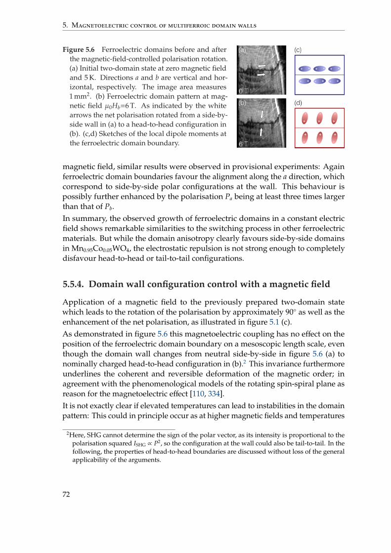
5. Magnetoelectric control of multiferroic domain walls
Figure 5.6 Ferroelectric domains before and afterthe magnetic-field-controlled polarisation rotation.(a) Initial two-domain state at zero magnetic fieldand 5 K. Directions a and b are vertical and hor-izontal, respectively. The image area measures1 mm2. (b) Ferroelectric domain pattern at mag-netic field µ0Hb=6 T. As indicated by the whitearrows the net polarisation rotated from a side-by-side wall in (a) to a head-to-head configuration in(b). (c,d) Sketches of the local dipole moments atthe ferroelectric domain boundary.
magnetic field, similar results were observed in provisional experiments: Againferroelectric domain boundaries favour the alignment along the a direction, whichcorrespond to side-by-side polar configurations at the wall. This behaviour ispossibly further enhanced by the polarisation Pa being at least three times largerthan that of Pb.In summary, the observed growth of ferroelectric domains in a constant electricfield shows remarkable similarities to the switching process in other ferroelectricmaterials. But while the domain anisotropy clearly favours side-by-side domainsin Mn0.95Co0.05WO4, the electrostatic repulsion is not strong enough to completelydisfavour head-to-head or tail-to-tail configurations.
5.5.4. Domain wall configuration control with a magnetic field
Application of a magnetic field to the previously prepared two-domain statewhich leads to the rotation of the polarisation by approximately 90◦ as well as theenhancement of the net polarisation, as illustrated in figure 5.1 (c).As demonstrated in figure 5.6 this magnetoelectric coupling has no effect on theposition of the ferroelectric domain boundary on a mesoscopic length scale, eventhough the domain wall changes from neutral side-by-side in figure 5.6 (a) tonominally charged head-to-head configuration in (b).2 This invariance furthermoreunderlines the coherent and reversible deformation of the magnetic order; inagreement with the phenomenological models of the rotating spin-spiral plane asreason for the magnetoelectric effect [110, 334].It is not exactly clear if elevated temperatures can lead to instabilities in the domainpattern: This could in principle occur as at higher magnetic fields and temperatures
2Here, SHG cannot determine the sign of the polar vector, as its intensity is proportional to thepolarisation squared ISHG ∝ P2, so the configuration at the wall could also be tail-to-tail. In thefollowing, the properties of head-to-head boundaries are discussed without loss of the generalapplicability of the arguments.
72

5.6. Domain boundaries in spin-spiral multiferroics
the magnitude of Pa is clearly larger than that of Pb [184]. On the other hand, theferroelectric domains exhibit a remarkable stability even in close proximity to TC.Finding a field and temperature regime where the domain pattern visibly changeswould give tremendous insight into the energy scales that determine the domainanisotropy and the effect of the depolarising field.In conclusion, the domains in multiferroic Mn0.95Co0.05WO4 clearly show a prefer-ence for side-by-side domain walls, as in conventional ferroelectrics, while showinga remarkable stability upon the magnetic-field-induced polarisation rotation. Thetransformation from uncharged side-by-side to nominally charged tail-to-tail do-main walls clearly underlines the induced ferroelectric character as well as thesmallness of P.Due to the close relationship between the spin order and the dipole moment, thelocal structure at the domain boundary deserves a closer look. In the followingsection, the micro-structure and physical properties of multiferroic domain wallsare discussed in more detail.
5.6. Domain boundaries in spin-spiral multiferroics
The multiferroic properties in spin-spiral multiferroics like MnWO4 or TbMnO3 areinduced by antisymmetric exchange between non-collinear spins, which relates thespiral handedness C = Si×S j with polar displacements, adding up to a macroscopicferroelectric moment [123, 137].Between domains of opposite polarisation, the chirality of the spin spiral mustchange. As already discussed in the PhD thesis of Tim Hoffmann [353], themost probable solution to this problem is the gradual rotation of the spin-spiralplane ℘ ⊥ C across the domain boundary. Here, only the magneto-crystallineanisotropy energy is paid, which typically is less than the energy scales related tothe exchange interaction. Since a magnetic field readily induced the rotation of thenet polarisation due to changes in the magnetic anisotropy in Mn0.95Co0.05WO4, is issimple to assume such rotations can readily occur due to local boundary conditions.Figure 5.7 illustrates the consequences of this idea: In bulk, the spin-spiral plane ℘lies in the xz plane, as illustrated by the circular discs. Across a domain boundary,℘ tilts towards the yz plane, and beyond, until it lies again in the xz plane. Tovisualise the twist from the front to the back of the plane, the opposite sides of ℘are coloured red and blue, respectively.If one assumes that the cycloidal spin spiral remains unaffected by the localorientation of the rotation plane ℘, in first order the magnitude of the local dipolesP will not change, but their direction will: Even within the boundary a modulatedpolarisation will be present, as shown by the green arrows in figure 5.7.
73

5. Magnetoelectric control of multiferroic domain walls
Figure 5.7. Schematic view on the microscopic structure of multiferroic domains wall:A favourable way to change the spin chirality C = Si × S j is to revert the direction ofthe spin plane ℘ ⊥ C, here shown as red and blue sides. As consequence, the localdipoles P (in green) also will be modulated across the wall. Depending on the direction,the ferroelectric character of the domain boundary will be different. Application of amagnetic field will lead to the rotation of the local anisotropy plane ℘ and thus changesthe direction of the polarisation within the domains and the domain boundary (far left).
The character of this multiferroic domain walls is different, depending on thedirection of the boundary normal n: Although the twist of the plane ℘ is the same inall three configurations, both ferroelectric Bloch and Néel walls can be stabilised.3
As a consequence of this complex microscopic structure, new physical propertiescan arise at the multiferroic boundaries. The major advantage of such effectsis related to the localised character of the interfaces, and their controllability byapplied fields, as demonstrated in the first part of the chapter.Charge and conductance As shown for conventional ferroelectric materials [322–
326], nominally charged head-to-head or tail-to-tail walls can induce localconductance. This effect depends on the electric depolarisation field ∝∆P⊥n · (ε0εr)−1, the dielectric constant εr, and the semiconducting properties
3The former is characterised by Pwall ⊥ n, while the latter has Pwall ‖ n.
74

5.6. Domain boundaries in spin-spiral multiferroics
leading to the screening of the charge accumulation at the boundary.4
Due to the predominance of side-by-side domain walls in Mn0.95Co0.05WO4
it seems that electrostatic repulsion indeed plays a sizeable role. Due to themagnetoelectric effect the character of the wall can be tuned, and thereforesimilar conducting properties also may be expected for this material.
Strain The gradients induced by the rotation of the polarisation across the domainboundary induce a local strain. While this does not reduce the net symmetry(which is already 1 in bulk Mn0.95Co0.05WO4), the local crystallographicstructure will be different than in the bulk domains and the gradient mightallow for flexoelectric couplings [355, 356]. Furthermore, local defects andstrain fields, e.g. induced by dislocations might lead to a stronger pinningof the domain walls which would influence their electric-field switchingbehaviour.
Interactions between domain boundaries The change of handedness in figure 5.7involves a rotation of the spin-spiral plane ℘. The interaction betweenneighbouring boundaries therefore depends on the relative orientation ofthis twist: Domain walls with opposite twist can merge, those with samecannot. This behaviour of avoiding and coalescent domain walls was alreadyobserved and discussed for domains in multiferroic MnWO4 [353].
5.6.1. Micro-magnetic model of domain walls in Mn0.95Co0.05WO4
To obtain a realistic understanding of the local magnetic and electric properties andthe involved length scales, micro-magnetic simulations can be used to calculate themicroscopic structure of a multiferroic domain wall. These results presented herewere obtained by Anders Bergman from Uppsala University (Sweden).Calculations Micro-magnetic and spin-dynamic simulations search for spatial mag-netisation distribution that minimise the total energy of the system [34, 357]. Con-tributing to this energy are Heisenberg exchange, magneto-crystalline anisotropy,and the Dzyaloshinskii-Moriya interaction.The coupling constants were calculated for Mn0.95Co0.05WO4 using density func-tional theory (DFT) [358]. Qualitatively equivalent interactions were also obtainedwith independent calculation methods (LDA+U). These values were then usedto solve the micro-magnetic equations. From the determined spin structure thepolarisation was calculated using the spin-current model [135].The balance of the exchange interactions stabilised a magnetic modulation vectorq = (0.17, 0.5, 0.41) in reasonable agreement with neutron scattering results [110,
4Although the polarisation in MnWO4 is approximately two to three orders of magnitude smallerthan in conventional ferroelectric materials as BaTiO3. But since εr is much smaller in MnWO4
the depolarising field differs by only one order of magnitude.
75

5. Magnetoelectric control of multiferroic domain walls
Figure 5.8. Profile of the polarisation contributions Pa, Pb and the net polarisation |Ptot|
along a calculated by micro-magnetic simulations: (a) At zero field side-by-side domainswith ferroelectric Bloch walls are favoured. The polarisation vector rotates within theab-plane and its value is enhanced in the middle of the boundary. (b) The state ofthe domain wall changes at high magnetic field to a head-to-head configuration. Thisboundary corresponds to a ferroelectric Néel wall, which is only half as wide as in thezero-field case. Contributions of polarisation Pc are negligible in both cases.
334]. Values for the magneto-crystalline anisotropy were adapted from [359, 360].The calculations lead to a ferroelectric state with a polarisation along b, whichvanishes above 15 K, again in valid agreement with observations [184].Since the simulations of a single-domain state coincide well with the multifer-roic properties of Mn0.95Co0.05WO4, meta-stable domain walls were introducedartificially by simulating a rapidly cooled hot disordered system with a size of200 × 24 × 24 unit cells. Relaxation of the spin system then lead to the determinationof the local magnetic and electric structure at the domain walls.Results At zero field, the calculations clearly showed a preference for side-by-sidedomain walls, as expected from the experiments. Furthermore, the simulation ofthe domain wall structure confirm the phenomenological model depicted figure 5.7:Indeed, the polarisation reversal across the domain boundary occurs as due to therotation of the spin plane. Consequently, an additional contribution Pa is inducesas the net polarisation rotates within the domain wall.The profile of the polarisation contributions Pb and Pa and the net polarisation |Pnet|
across the wall is shown in figure 5.8 (a): While Pb changes sign, a sizeable amountof Pa is induced. The net polarisation thus varies strongly and is enhanced in themiddle of the wall, Pwall/Pbulk ≈ 2.8. The width of the boundary wFWHM ≈ 10 nmlies well between values of ferroelectric and ferromagnetic domain walls [201, 320].Micro-magnetic calculations also allow to determine the spin and electric structureafter the magnetic-field-induced polarisation rotation: In this case the side-by-sideBloch wall transforms to a head-to-head Néel wall. The local polarisation profileis shown in figure 5.8 (b): While Pa changes sign, the polarisation vector rotatestowards the b direction. In agreement with observations in Mn0.95Co0.05WO4, thepolarisation value Pa within the domain exceeds that of Pb [184]. As consequence,
76

5.7. Conclusions and perspectives
the net polarisation is slightly reduced within the domain boundary Pwall/Pbulk ≈ 0.8.Interestingly, this wall is only half as wide as in the zero-field configuration.Conclusion These calculations obviously show that the micro-structure of multi-ferroic domain walls differ to that of the bulk compound. This can enable newemergent phenomena, as discussed previously. The narrow boundaries in multi-ferroic Mn0.95Co0.05WO4 therefore allow for localised properties which are readilytunable by electric and magnetic fields.
5.7. Conclusions and perspectives
Here, the full control of the domain boundary position and polarisation state inby electric and magnetic fields was demonstrated in multiferroic Mn0.95Co0.05WO4.This tuneability allows to change from favourable side-by-side ferroelectric domainboundaries to nominally charged head-to-head configuration. The microscopicstructure of such multiferroic domain walls were discussed on a phenomenologicallevel and on the basis of micro-magnetic simulations.These results lay the foundation for future experiments using microscopic probeslike piezo force microscopy [361], spin-polarised scanning microscopy [362, 363],and low-energy and photo-emission electron spectroscopy [94, 364, 365]: Such tech-niques can be used to investigate the microscopic structure and physical propertiesof the domain boundary itself while controlling its position and configuration stateby applied electric and magnetic fields, respectively.
77


6. Magnetoelectric polarization flipin multiferroic Mn2GeO4
Magnetic olivine Mn2GeO4 is one of the rare multiferroicmaterials which exhibit both a spontaneous polarisation aswell as a finite magnetisation. Furthermore, there exists aclose cross-correlation between them: With the application of
a magnetic field not only the ferromagnetic moment is switched, but thesign of the spontaneous polarisation reverses as well.Here, optical second harmonic generation is used to investigate theferroelectric domain distribution in Mn2GeO4 and its dependence onapplied electric and magnetic fields. The results clearly show thatthe unusual magnetoelectric effect originates from the direct couplingbetween mobile ferromagnetic domains and robust polarisation domains.This allows for the hysteretic control of a ferroelectric domain state bymeans of a magnetic field.
In many spin-spiral multiferroics the magnetoelectric properties are promoted bycompeting magnetic interactions, and therefore crystallographic structures withgeometrically frustrated exchange paths might enable new cross-couplings.An example for such complexity is the olivine structure, which features zigzagchains, and distinct crystallographic sites enabling magnetic frustration [111].Indeed, Cr2BeO4 was the first spin-spiral ferroelectric to be found [366, 367]. RecentlyMn2GeO4 attracted attention, too, due to its unusual multiferroic properties [172,368, 369]; since few materials are known exhibiting both a spontaneous polarisationas well as a magnetisation. In Mn2GeO4 these moments also exhibit a very closecross-correlation, as ferroelectric and ferromagnetic hysteresis show simultaneousswitching under an applied magnetic field.So far, the spatially-resolved behaviour of the ferroic domains under applied fieldshas not been discussed. Here, the distribution and field-dependence of multiferroicdomains in Mn2GeO4 are investigated using optical SHG.
79
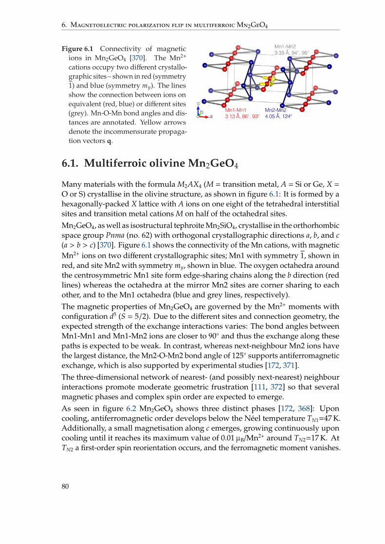
6. Magnetoelectric polarization flip in multiferroicMn2GeO4
Figure 6.1 Connectivity of magneticions in Mn2GeO4 [370]. The Mn2+
cations occupy two different crystallo-graphic sites – shown in red (symmetry1) and blue (symmetry my). The linesshow the connection between ions onequivalent (red, blue) or different sites(grey). Mn-O-Mn bond angles and dis-tances are annotated. Yellow arrowsdenote the incommensurate propaga-tion vectors q.
6.1. Multiferroic olivine Mn2GeO4
Many materials with the formula M2AX4 (M = transition metal, A = Si or Ge, X =
O or S) crystallise in the olivine structure, as shown in figure 6.1: It is formed by ahexagonally-packed X lattice with A ions on one eight of the tetrahedral interstitialsites and transition metal cations M on half of the octahedral sites.Mn2GeO4, as well as isostructural tephroite Mn2SiO4, crystallise in the orthorhombicspace group Pnma (no. 62) with orthogonal crystallographic directions a, b, and c(a > b > c) [370]. Figure 6.1 shows the connectivity of the Mn cations, with magneticMn2+ ions on two different crystallographic sites; Mn1 with symmetry 1, shown inred, and site Mn2 with symmetry my, shown in blue. The oxygen octahedra aroundthe centrosymmetric Mn1 site form edge-sharing chains along the b direction (redlines) whereas the octahedra at the mirror Mn2 sites are corner sharing to eachother, and to the Mn1 octahedra (blue and grey lines, respectively).The magnetic properties of Mn2GeO4 are governed by the Mn2+ moments withconfiguration d5 (S = 5/2). Due to the different sites and connection geometry, theexpected strength of the exchange interactions varies: The bond angles betweenMn1-Mn1 and Mn1-Mn2 ions are closer to 90◦ and thus the exchange along thesepaths is expected to be weak. In contrast, whereas next-neighbour Mn2 ions havethe largest distance, the Mn2-O-Mn2 bond angle of 125◦ supports antiferromagneticexchange, which is also supported by experimental studies [172, 371].The three-dimensional network of nearest- (and possibly next-nearest) neighbourinteractions promote moderate geometric frustration [111, 372] so that severalmagnetic phases and complex spin order are expected to emerge.As seen in figure 6.2 Mn2GeO4 shows three distinct phases [172, 368]: Uponcooling, antiferromagnetic order develops below the Néel temperature TN1=47 K.Additionally, a small magnetisation along c emerges, growing continuously uponcooling until it reaches its maximum value of 0.01µB/Mn2+ around TN2=17 K. AtTN2 a first-order spin reorientation occurs, and the ferromagnetic moment vanishes.
80

6.1. Multiferroic olivineMn2GeO4
Figure 6.2. Multiferroic phase diagram of Mn2GeO4: Three phases with different antifer-romagnetic order are distinguished. The Néel transition at TN1 is second-order, whereasthe transitions at TN2 and TC are of first-order character. Only the incommensurate phasebelow TC shows ferroelectric properties with P ‖M ‖ c. Adapted from [172, 368].
Above TC=6 K the magnetic order preserves the unit cell (q = 0), and the momentslie either along the a (TN2 < T < TN1) or b direction (TC < T < TN2) [172]. Due tothe different symmetry of the crystallographic Mn1 and Mn2 sites though, bothmagnetic anisotropy and amount of ordered moment can be different [373, 374].At TC another first-order transition leads to the incommensurate low-temperaturephase. The magnetic propagation vector q = (0.211, 0.136, 0) lies in the ab-planeand is almost parallel to the Mn1-Mn2-Mn1 zigzag bonds.1
The low-temperature phase of Mn2GeO4 exhibits a complex magnetic order as wellas multiferroic properties with both a finite magnetisation M||c and a spontaneouspolarisation P||c with magnitude Pc=6µC/m2. Several experiments with varyingtemperature, magnetic field, and pressure imply that these moments are inducedby the underlying antiferromagnetic order, i.e., have a common microscopic origin[172, 368, 369, 375] possibly related to antisymmetric exchange interactions.While both the polarisation and magnetisation are exceedingly small in Mn2GeO4,2
they show a remarkable and robust cross-coupling: A magnetic field in the orderof 100 mT not only reverses the magnetisation Mc, but also the sign of ferroelectricPc [172]. This hysteresis-locking does not imply a one-to-one coupling between Mc
and Pc, however, and its underlying mechanism is not yet entirely clear.So far the multiferroic and magnetoelectric properties of Mn2GeO4 were investigatedwith integrated methods. The goal of this chapter therefore is to elucidate themultiferroic properties of Mn2GeO4 on mesoscopic length scales and the effect ofboth electric and magnetic fields on the domain population.
1The incommensurate wave vector q = (u, v, 0) has point group symmetry mc. Therefore, fourdifferent translation domains corresponding to the equivalent directions of the wave vector starq∗ = {(u, v, 0), (u, v, 0), (u, v, 0), (u, v, 0)} are possible. The different directions of q are depicted bythe yellow arrows in figure 6.1.
2The spontaneous polarisation in Mn2GeO4 is two orders of magnitude smaller than in thespin-spiral ferroelectric materials MnWO4 or TbMn2O5. The magnetisation value of 0.01µB perMn ion corresponds to less than 2 %� of the net moment, or a spin canting angle of less than 0.1◦.
81

6. Magnetoelectric polarization flip in multiferroicMn2GeO4
Figure 6.3 Investigation of the a-cut sam-ple was performed in normal incidence(a), with light polarisation along b and cin the imaging plane (b). The c-cut sam-ple had to be rotated in the beam to exciteSHG contribution χcbb (c,d).
6.2. Experimental details
Before discussing the results of the imaging experiments, the following sectionbriefly describes details of sample preparation, the setup used for the SHG experi-ments, and the challenge of applying high voltages at low temperatures.Sample preparation Large Mn2GeO4 single crystals were grown by the floatingzone method, and provided by T. Honda (Kimura group, Osaka University, Japan).For optical experiments a- and c-cut samples between 1 mm and 50µm thicknesswere used, which were lapped and polished with silica slurry (Ultrasol 555).The obtained sample surfaces were optically flat. The c-cut platelets, however, showfanning cracks mainly along b in agreement with moderate cleavage expected alongthis direction [376]. These cracks strongly absorb light and diminish the effectivearea that can be used for optical experiments. Furthermore, selective etching wasobserved at these cracks during mechanical-chemical polishing.SHG experiment The SHG data was acquired using the transmission setup de-scribed in section 3.4, using 120 fs laser pulses as coherent light source. The incidentpower was in the range 20µJ to 25µJ, and the beam was slightly defocussed toilluminate the whole sample area up to 3 mm2. The signal acquisition was eitherintegrated, or spatially resolved for domain imaging.Sample environment The sample was located in a magnet cryostat, allowingtemperatures down to 2 K. The magnetic field was applied along the c direction.Furthermore, electric fields were applied along c, using either metal electrodes inthe case of a-cut or grown-on ITO electrodes on c-cut samples.3
Imaging planes As shown in figure 6.3 the experiments were performed in trans-mission on the ab- and bc-planes. The a-cut sample was imaged in normal incidence.In contrast, the c-cut sample was slightly rotated in the beam by 20◦ to 35◦ in orderto get a projection of the second harmonic response proportional to χcbb. In spiteof this experimental geometry, no depth interference between stacked domainswas observed for a thin sample. The SHG images therefore reflect the domainanisotropy in the bc- and ab-plane, respectively.
3Metal electrodes for the a-cut sample only allows to apply fields of up to 1.5 kV/mm, which is toosmall to affect the ferroelectric domain structure but useful to distinguish different polarisationdomains via interference with an EFISH signal. On the thin Mn2GeO4 c-cut platelet electricfields of up to 15 kV/mm could be achieved using ITO electrodes (see section 3.6.2).
82
6.3. Optical properties ofMn2GeO4
Low-temperature measurements Temperature control proved to be challengingdue to the low multiferroic transition temperature and continuous laser heating;problems occurred in combination with applied electric fields, particularly as thebulky sample holder hinders efficient cooling in the He gas flow. Unfortunately,measuring in liquid helium was not an option, as the cryostat had a cold leak –flooding with suprafluid LHe would have solved the aforementioned problems.Normal liquid helium continuously boils, which makes optical measurementsimpossible. To avoid bubbles, the variable temperature insert can be pumped,leading to a gas atmosphere of lower pressure and temperature. This, in turn,reduces electrical breakthrough and limits the electric field that can be applied.Therefore, a tight trade-off between laser power, needle-valve temperature andopening, He gas pressure, and electric fields was required.4 Under these circum-stances, controlled field-cooling experiments were difficult, especially as the coolingrate becomes discontinuous around 4.2 K.
6.3. Optical properties of Mn2GeO4
To determine spectral regions of interest, polarised linear absorption spectra weremeasured, as presented in figure 6.4 (a): While dd transitions are spin-forbiddenfor the case of 3d5 configuration, the thin platelets of Mn2GeO4 appeared reddishbrown in transmission, which is actually is quite common for materials containingMn2+ or Fe3+ cations [106]. This is mainly due to the long tail of the lowest-lyingMn→O charge-transfer transition in the UV region extending to the visible rangeof the spectrum.Crystal-field transitions Furthermore, in all three spectra weak crystal-field tran-sitions are observed as marked in figure 6.4 (a). Absorption for c-polarised lightis strongest throughout the visible regime, while a- and b-polarised bands appearweaker. Careful peak analysis revealed five dd transitions in each spectrum, andan additional peak in the c-polarised spectrum. Position, width, and intensity ofthe peaks are summarised in table 6.5. The different absorption results in opticaldichroism of Mn2GeO4 as depicted in the upper left corner of figure 6.4 (a).5
The assignment to possible crystal-field transitions as summarised in Tanabe-Sugano diagrams [104, 105] is achieved in comparison with isostructural tephroite
4A good, but not fool-proof way to get to suitable low temperatures in gas atmosphere is to startpumping the sample room at 10 K, and adapt the needle valve such that the gas pressure staysabove 800 mT and the heater power is at least 30 %. Then the sample can be slowly cooled down.Flooding with LHe still occurred more often than not. Thankfully, this is detected easily byvisual observation; but it takes some time to evaporate the liquid once it is in the sample room.
5Thanks to Franziska Schlich (Laboratory for Nanometallurgy, ETH Zürich) for simulating theabsorption colours for Mn2GeO4 and Mn0.95Co0.05WO4 (see also figure 5.2).
83

6. Magnetoelectric polarization flip in multiferroicMn2GeO4
Figure 6.4. Optical properties of Mn2GeO4. (a) Linearly polarised spectra measured atroom temperature. The mean peak position and width of the detected crystal-fieldtransitions #1-#4 are marked, for detailed assignment see table 6.5. The blue area denotesthe spectral dependence of the SHG peak around 1.9 eV. The upper left corner shows thesimulated pleochroism of a 250µm thick Mn2GeO4 sample. (b) Angular dependence ofabsorption coefficient α in the bc-plane (dots), which shows a deviation from the ellipsoidexpected for an orthorhombic material (line).
Mn2SiO4 [106]. Compared to Mn2GeO4 the crystal-field splitting in Mn2SiO4 isslightly stronger, probably attributed to the different lattice constants [370, 376].The Mn sites with different symmetry contribute differently to the optical absorption;spin-forbidden transitions in centrosymmetric Mn1 sites will only be enabled byvibronic coupling. In contrast, selection rules are less strict for transitions atthe acentric Mn2 octahedra, and light-matter couplings are further enhanced byantiferromagnetic interactions. Thus the optical absorption by Mn2 ions is expectedbe stronger and to show a more pronounced polarisation dependence than that ofthe Mn1 cations. The definite assignment of bands to different sites can only bemade using temperature-dependent spectral measurements, however [266].Low-energy transition and anomaluous polarisation dependence Of particularinterest is the lowest-lying transition at 1.76 eV which is observed in the c-polarisedspectra only and cannot be assigned to a crystal-field transition. It might be dueto a further splitting of electronic levels at the low-symmetry Mn sites. At similarenergies an anomalous polarisation dependence of the absorption is also observed,as seen in figure 6.4 (b): Although orthorhombic symmetry implies the absorptionellipse to be aligned along the crystallographic directions, the angular dependenceof α(~ω) has an additional contribution for light polarisation along the bc diagonals.Possibly this odd behaviour is linked to a spin-flip transition between two ions,coupled by antiferromagnetic exchange, as observed for coloured sapphire [377].Further indicators for this theory are the approximate diagonal alignment of theMn2-O-Mn2 bonds in the bc-plane and their strong anti-parallel spin coupling inthe magnetically ordered phases [172, 371]. Again, temperature-dependent spectralmeasurements could clarify this assignment.
84

6.3. Optical properties ofMn2GeO4
band a b c
CT Ec (eV) 3.716 3.638 3.861 Metal-oxygen charge transfertransition dominating UV andVIS absorption. Was subtractedbefore performing analysis.
A (m−1) 77364 49271 102906FWHM (eV) 0.482 0.432 0.626y0 (m−1) 8821 10623 11069
y′0 (m−1) 1393 1146 2310 Background for multi-Gauss fit.
#0 Ec (eV) – – 1.760 Cannot be attributed to a ddtransition.A (m−1) – – 271
FWHM (eV) – – 0.205
#1 Ec (eV) 2.172 2.177 2.103 6A1g →4 T1g.
A (m−1) 1090 1017 2025FWHM (eV) 0.398 0.474 0.339
#2 Ec (eV) 2.784 3.672 2.755 6A1g →4 T2g.
A (m−1) 4360 2406 7955FWHM (eV) 0.690 0.576 0.815
#3 Ec (eV) 2.990 3.000 2.990 6A1g →4 Eg,4 A1g. Very sharp,
and independent of crystal fieldsplitting energy.
A (m−1) 681 621 948FWHM (eV) 0.116 0.122 0.118
#3′ Ec (eV) 3.090 – 3.106 Occurs as shoulder to thewell-defined peak #3. Probably6A1g →
4 Eg.A (m−1) 264 – 201FWHM (eV) 0.163 – 0.129
#4′ Ec (eV) – 3.262 –A (m−1) – (6160) –FWHM (eV) – (0.850) –
#4 Ec (eV) 3.375 3.387 3.419 6A1g →4 T2g.
A (m−1) 1843 (101) 2159FWHM (eV) 0.357 (0.080) 0.380
Table 6.5. Assignment of optical transitions for the absorption spectra of Mn2GeO4 shownin figure 6.4. Charge-transfer (CT) and crystal-field transitions (#i) were fitted withGaussian functions using the Peak Analyser of the data analysis software OriginLab[271]. Assignment to crystal-field transitions were compared with isostructural tephroiteMn2SiO4 [106]. As the high-energy transitions are almost hidden in the charge-transferabsorption, the fit parameters in brackets are unreliable.
85

6. Magnetoelectric polarization flip in multiferroicMn2GeO4
Figure 6.6. Rotational SHG anisotropies for a-cut and c-cut samples of Mn2GeO4
(2~ω ≈1.9 eV). (a,b) Anisotropy 0◦ with S(2ω)||E(ω) coupling to χbbc for k||a, and thestructure projected in this direction. (c,d) Anisotropy 90◦ with S(2ω) ⊥ E(ω) in slightlyrotated c-cut sample, leading to the observation of SH contribution χcbb and the crystalstructure viewed in this direction. (e) Temperature-dependence of the SHG signalχcbb ∝ Pc at 1.9 eV. Due to laser heating, the transition temperature is slightly lower thanits literature value of 6 K [172, 368].
SHG contribution This low-energy transition might only seem like a minor detail.But the search for a non-linear response of Mn2GeO4 in the range of 1.5 eV to 3.3 eVlead to only one SHG contribution around 1.9 eV.6
SHG selection rules imply that electric-dipole SHG contributions χi jk are onlyallowed in the non-centrosymmetric phase, with an odd number of the polardirection c in the indices i, j, k. This agrees with the angular dependence of themultiferroic SHG signals in figure 6.6 (a,c). Interestingly, while in a c-cut sampleχcbb is observed, the a-cut sample shows a χbbc signal. This is peculiar, becauseSHG contributions of the type χcbb would be allowed for k ‖ a. Comparison of theangular SHG dependence with the crystal structure in figure 6.6 (b,d) again impliesa close relationship between (non-)linear response and the Mn2-Mn2 bonds.The SHG signal at 1.9 eV was observed in the non-centrosymmetric multiferroicphase only. Temperature-dependent measurements as shown in figure 6.6 (e)demonstrate the jump-like emergence at the first-order transition TC ≈ 6 K, andthe constant intensity in the multiferroic phases is similar to the temperature-dependence of the spontaneous polarisation [172]. Together with the magnetic-and electric-field-dependent behaviour of the domain images it can be concludedthat the SHG contributions χbbc and χbcc couple to ferroelectric Pc only.
There are three macroscopic order parameters in the low-temperature phase – thepolarisation P, the magnetisation M, and the antiferromagnetic component L′ whichdetermines the relative sign of M and P. In principle, the SHG signal can couple toone or more order parameters. Apart from the coupling term χSHG ∝ P the other sixpossibilities can be discarded, however:
6In a one mm thick c-cut sample the SHG response peaked at 1.82 eV, but for the other sampleswith thickness from 50µm to 250µm a signal centred around 1.9 eV was observed.
86

6.4. Imaging of multiferroic domains inMn2GeO4
In the case of SHG coupling to M a non-zero signal would be expected in the otherweakly ferromagnetic phase between 17 K and 47 K, but was not observed.
Coupling to either L′, PM, or PML′ cannot explain the SHG contrast reversal with amagnetic field shown in figure 6.9 as those products stay unaffected by ±M→ ∓M.
Finally, the demonstration of electric-field poling also excludes SHG coupling to ML′ orPL′: In neither case the observation of a single-domain state indicated by the uniformbrightness in figure 6.7 (a) and its subsequent fragmentation with applied magneticfield – demonstrating an uneven distribution of L′ – can be explained.
Electric-field induced SHG Application of an electric field E||c also leads to aninduced SHG signal, even above both the Curie and the Néel temperatures TC, TN.Its spectral and polarisation dependence is exactly that of the ferroelectric signal,which might imply a related microscopic origin. This notion is emphasized by thefact that the ratio between ferroelectric and EFiSH signal is in the same order ofmagnitude as the ratio between spontaneous Pc and induced ε0εrEc.Together with the aforementioned preference of the incident light polarisation to lieparallel to the Mn2-Mn2 bonds, both spontaneous and induced polarisation mightbe due to a coherent charge displacement on the zigzag chains in the bc plane [372].Other non-linear contributions Higher-order non-linear responses independentof magnetic order were found at 2.67 eV,7 and for energies above 3.2 eV (possiblyinvolving non-linear interactions with the lowest-lying Mn→O transition [214]).
6.4. Imaging of multiferroic domains in Mn2GeO4
The following experiments focus on the imaging of the multiferroic domain structure,and its behaviour under applied electric and magnetic fields. Of interest are thechanges that accompany the synchronised ferromagnetic and ferroelectric switching,especially for a multi-domain state; here, spatially resolved measurements canunambiguously decide if the magnetoelectric coupling in Mn2GeO4 involves achange of the ferroelectric domain pattern or not.SHG imaging Although the magnitude of the polarisation in Mn2GeO4 is verysmall, the SHG contribution coupling to Pc was strong enough to get satisfactorydomain images using relatively short exposure times of 20 seconds to 120 seconds.The image quality was further enhanced by suppressing fluorescent backgroundsignals with an interference filter at the SHG central wavelength (1.9 eV � 650 nm).The magnification was approximately 6µm/px in all experiments.
87

6. Magnetoelectric polarization flip in multiferroicMn2GeO4
Figure 6.7. Electric-field switching in Mn2GeO4. (a) Image sequence with increasingelectric field Ec applied on a c-cut sample. The overlap of the ITO electrodes is marked bya white outline. Numbers give magnitude of E||c in kV/mm. (b) Area fraction of brightdomains in the region of electrode overlap against electric field. The line is a guide to theeye, and shows the onset of ferroelectric switching around fields of 5 kV/mm, which is alower bound for the coercive field.
6.4.1. Electric-field control of the ferroelectric domains
First, the electric-field control of the induced polarisation is demonstrated in a c-cutMn2GeO4-sample. The first image in figure 6.7 (a) shows the ferroelectric domainpattern after zero-field cooling. Domains of different polarity are distinguishedby their brightness, and show a pattern of stripes with typical thickness 20µm to40µm mostly aligned along the vertical b direction or slightly inclined to it.Application of an electric field of sufficient strength leads to ferroelectric switchinggoverned by the growth of bright and the shrinking of dark domains; until athigh fields a ferroelectric single-domain state indicated by uniform brightness inreached. The electric-field switching process only happens where the front andback ITO electrodes overlap, which is indicated by a white outline in figure 6.7 (a).Furthermore, an EFISH signal leads to the apparent brightness decrease in theareas without electrode overlap, however, the domains in these regions stay mostlyunaffected by the applied electric field.The temporal resolution for the switching process, shown in figure 6.7 (a), isseemingly governed by domain growth and not nucleation, and the boundary prop-agation occurs along two main directions: The main motion is downwards along b,probably enhanced by the thermal gradient. A sideways motion perpendicular tothe slightly diagonal domain boundaries is also observed.
7Three-photon fluorescence involving the dd transition #2, similar to that found in Mn0.95Co0.05WO4.
88

6.4. Imaging of multiferroic domains inMn2GeO4
Figure 6.8. Magnetic-field dependence of domain distribution in the ab plane. The imagesequence shows the evolution of a single-M-multi-P-domain state under the reversal of amagnetic field H = 0.94Hc + 0.34Ha. Although changes occur for fields around 60 mT, theinitial and final domain state strongly resemble each other, underlining the robustness ofthe polarisation domain pattern to magnetic fields.
Figure 6.7 (b) shows the area fraction of bright domains, reminiscent of the initialcurve of a full hysteresis loop. The increase for electric fields above 5 kV/mm givesa lower bound to the coercive field. The high field strength needed to switch theferroelectric polarisation in Mn2GeO4 is probably due to the induced character andsmall magnitude of the ferroelectric polarisation.Application of electric fields above 8 kV/mm often were accompanied by dischargingcurrents and sparks. These would inevitably change the ferroelectric domaindistribution by rapid heating and quenching, and lead to very small-scale domainpatterns. As the ITO electrode areas were not symmetric to each other, break-through was also asymmetric with positive and negative voltages. Therefore a fullferroelectric hysteresis loop could not be obtained in these experiments.
6.4.2. Behaviour of the domain pattern under magnetic fields
The experiments described in the following section focus on the magnetic-field-dependence of the ferroelectric domain pattern to better understand the unusualmagnetoelectric coupling: As demonstrated by integrated hysteresis measurements,the weak magnetisation and the spontaneous polarisation switch simultaneouslyfor small fields of about 100 mT [172].Magnetic-field dependence in c-cut sample Figure 6.8 shows the evolution ofa single-M-multi-P-domain state upon reversal of the magnetic field Hc. Here,changes occur especially for fields of 30 mT to 90 mT, as additional stripe-like
89

6. Magnetoelectric polarization flip in multiferroicMn2GeO4
Figure 6.9. Magnetic-field dependence of domain distribution in the bc plane. (a) Thediagram shows the integrated intensity of the SHG interference signal | ± P + E|2, and thetime series corresponds to the unfolding of a full hysteresis loop. Images (b)-(g) showthe domain distribution before and after the three magnetic-field cycles. Domains ofopposite polarity are marked by a yellow or blue overlay. Axes b and c are oriented alongthe vertical and horizontal direction, respectively. The scale bar in (b) measures 500µm.
domains along b appear and move downwards. Therefore, the magnetic field caninduce additional ferroelectric domain walls in Mn2GeO4.The overall effect of the magnetic switching on the ferroelectric domain patternis minimal, however: Comparison of the first and last image of the sequencein figure 6.8 reveals only little changes. These images correspond to magneticsingle-domain states with −Mc and +Mc, respectively. As the spatial distributionshows only little changes, the magnetic-field-induced polarisation reversal does notaffect the ferroelectric domains much. Therefore, the intermediate domain imagesreflect a superposition of electric and magnetic domains.Furthermore, application of a magnetic field on a multi-Mc-single-Pc-domain state(obtained after zero-field cooling and subsequent electric-field switching) leadsto a break-up of the single-domain state into several polarisation domains (notshown). This demonstrates that the magnetisation reversal has a direct effect uponthe ferroelectric domains.Magnetic-field dependence in a-cut sample To further investigate this magnetic-field-induced polarisation flip similar experiments were performed with an a-cutsample, and electric-field induced SHG (EFISH) was used to generate a contrastbetween domains of opposite polarity ±Pc via I± ∝ |χ(±Pc + Ec)|2.Figure 6.9 shows both the integrated SHG intensity (a), as well as selected domainimages (b-g) with applied magnetic field Hc. Both trace the changes in ferroelectricdomain pattern starting from a multi-Mc multi-Pc-domain state. Figure 6.9 (a)resembles an unfolded hysteresis curve of the integrated SHG intensity, and showsrapid changes around Hc ≈ 60 mT upon the reversal of the magnetic field. Theimage sequence in figure 6.9 (b-g) shows the domain pattern of at different applied
90

6.4. Imaging of multiferroic domains inMn2GeO4
fields starting from a multi-Mc multi-Pc-domain state. By comparing images withand without EFISH contrast, domains of opposite polarity ±Pc can be distinguished,and are marked blue and yellow, respectively.8
Before discussing the particular behaviour of the first two magnetic-field cyclesit should be noted that the result of the third (and actually every following) fieldcycle confirms the behaviour already anticipated from the previously presentedresults: The coherent polarisation reversal with the magnetisation switching occurswithout disturbing the ferroelectric domain pattern; and is unambiguously shownby the interchanging of blue and yellow regions in figure 6.9 (f,g).As the first field cycle shown in figure 6.9 starts from a multi-Mc-domain state, theoverall spatial distribution is expected to change more upon the initial field cycle.The images 6.9 (b,c) clearly demonstrate this behaviour, with changes in colour(i.e. sign of Pc), alignment, and size of the domains with the initial field sweep to asingle-Mc-domain state.Curiously, upon the first magnetisation reversal +Mc → −Mc, the domain patterncan again change, as shown in figure 6.9 (d,e). As a consequence, domain boundariesstraighten out and smaller domains disappear. This effect cannot be directlyassociated to the magnetoelectric coupling, as the domain pattern stays robust forfurther field cycles. Therefore, the observed changes could rather be related to thefact that the system tries to adopt a domain pattern better suited to the spontaneouspolarisation along c. The value of Pc is small, but the sudden change by twice itsmagnitude might be large enough to induce adjustments in the spatial distributionof ferroelectric domains.In contrast, when starting from a single-Mc state obtained after magnetic-fieldcooling or a full hysteresis sweep, only the polarisation flips ±Pc → ∓Pc and withmerely small changes in the position of the domain walls, as discussed for figure 6.8or figure 6.9 (f,g). This effect is highly repeatable, and the domain distributionbetween different cycles show none or only minor differences.
6.4.3. Topography of ferroelectric and ferromagnetic domains
Since domain images in both the ab and bc plane were investigated, a typicalthree-dimensional distribution of ferroelectric and ferromagnetic domains can bepredicted, as shown in figure 6.10. Such an assignment can be used to determineaverage domain volumes; and the anisotropy reflects directions of preferredinteractions [34, 289].As can already be seen from figures 6.7 to 6.9 the ferroelectric – and ferromagnetic –domains in Mn2GeO4 align along preferred directions; however, the association
8To generate a domain contrast a field of Ec ≈ 0.6 kV/mm was applied, which is too low to affectthe ferroelectric domain pattern in Mn2GeO4.
91

6. Magnetoelectric polarization flip in multiferroicMn2GeO4
Figure 6.10 Spatial anisotropy of(a) ferroelectric and (b) ferro-magnetic domains in Mn2GeO4.The domain distribution in theac plane has not been inves-tigated. The cubes measure1 cm × 1 cm × 1 cm.
with crystallographic orientations is not very strict, as angles show a standarddeviation of about 10◦.Ferroelectric domains Figure 6.10 (a) shows the ferroelectric domain distribution,obtained by images of single-Mc domain states: On the polar ab face the domainboundaries align preferably parallel to b or inclined by about 30◦ to b. The ac faceshows preferred directions along c and at an angle of 10◦ to 30◦ towards b.Ferroelectric domain boundaries along the polar direction c are uncharged, andthus cost less energy. In contrast, the diagonal direction might reflect eitherthe structural zigzag chains shown in figure 6.1, the direction of the magneticmodulation vector ∠(−q, b) ≈ 33◦, or the spin direction in the multiferroic phase[172]. Any of these three properties are expected to be related to the inducedferroelectricity in Mn2GeO4 and thus could influence the domain anisotropy.Ferromagnetic domains Although SHG couples to the polarisation only, the ferro-magnetic domain pattern shown in figure 6.10 (b) could be determined using theindirect evidence from the intrinsic magnetoelectric coupling: In figure 6.8 the localpolarisation reversal during a magnetic-field sweep indicates stripe-like magnetisa-tion domains on the ab plane. The domain pattern in the ac plane can be deducedby comparing the domain contrast between the multi-Mc and single-Mc domainstates in figure 6.9 (b,c). In this case, the domain boundaries prefer directions of 45◦
or 30◦ to the b direction.The three-dimensional distribution of ferromagnetic domains in figure 6.10 (b) mightnot be truly accurate, since it compares apples to oranges – domain distributionscan adopt different anisotropies for zero-field cooling and after field sweeps [353,378]. As the field range ∆H for magnetic switching is rather narrow, and the domainchanges are not resolved in this image series, a similar assignment could not bemade in the case of the a-cut sample.
6.5. Magnetoelectric coupling in Mn2GeO4
With the experimental results described in the previous section it is possible toderive a conceptional understanding of the magnetoelectric effect in Mn2GeO4.As shown in figures 6.8 and 6.9, the coupled ferromagnetic and ferroelectric
92
6.5. Magnetoelectric coupling inMn2GeO4
hysteresis demonstrated by macroscopic measurements [172] is governed bya coherent flip of the polarisation ±Pc ↔ ∓Pc as the magnetisation reverses+Mc ↔ −Mc.Field dependence of domain pattern This magnetoelectric coupling leaves theferroelectric domain distribution mostly unchanged, provided that the sample hadbeen in a Mc-single-domain state prior to the application of the magnetic field.Due to the persistence of the magnetic-field-induced polarisation reversal even afterthe field is switched off, e.g. shown in figure 6.9 (e-g), the sign of the polarisation Pc
is indeed coupled to the internal magnetisation Mc and not the applied field Hc.When changing a multi-Mc to a single-Mc-domain state the final ferroelectricdomain distribution is determined by both the initial Pc and Mc states: On one hand,comparison of the images figure 6.9 (b,c) implies that after zero-field cooling Pc andMc domains show a distinct distribution. On the other hand, it was also observedthat a single-Pc-domain state fractioned into several polarisation domains due toan initial non-uniform sample magnetisation. Therefore, the first magnetic-fieldsweep leads to a rearrangement of the ferroelectric domains as the polarisationonly changes sign where the magnetisation does, too.In fact, only the rigid locking of ferroelectric and ferromagnetic domains can explainthe observed coupled ferroic hysteresis: From the results in figures 6.7 and 6.8 itis clear that magnetic and electric domain walls show different dynamics in anapplied field. If the polarisation domains would move in a magnetic field, too, andnot only locally revert their sign, one could expect changes in the domain pattern,leading to non-equal magnetic and electric hysteresis loops.Magnetoelectric coupling Thus the magnetic-field induced local polarisationflipping in Mn2GeO4 observed by macroscopic measurements [172], is shownto be coherent on mesoscopic scales, too. On a phenomenological level thismagnetoelectric effect must be described by a coupling linear in both Pc and Mc,since a quadratic dependence would not be sensitive to the relative orientation.To satisfy the symmetry of the free energy under both time reversal and spatialinversion, the coupling invariant Fme must also involve a polar magnetic term L′
which transforms like the irreducible representation Γ′2 (see table 6.11):
Fme ∝ PcMcL′ (6.1)
The parallel or anti-parallel alignment of Pc and Mc is determined by the sign ofpersistent L′, and thus preserved in the case of magnetic-field switching, wherethe magnetisation and the polarisation are simultaneously reversed.This coupling arises from the complex microscopic interactions in Mn2GeO4, whichpermit the emergence of both ferromagnetic and ferroelectric order induced bythe underlying the antiferromagnetic structure. In the PhD thesis of T. Honda[375] the origin of both Mc and Pc is discussed to be induced by a spin spiral with
93

6. Magnetoelectric polarization flip in multiferroicMn2GeO4
1 2a 2b 2c 1 ma mb mc 1′
Γ1 1 1 1 1 1 1 1 1 1 σii
Γ2 1 1 1 1 −1 −1 −1 −1 1 abcΓ3 1 1 −1 −1 1 1 −1 −1 1 σbc
Γ4 1 1 −1 −1 −1 −1 1 1 1 Pa
Γ5 1 −1 1 −1 1 −1 1 −1 1 σac
Γ6 1 −1 1 −1 −1 1 −1 1 1 Pb
Γ7 1 −1 −1 1 1 −1 −1 1 1 σab
Γ8 1 −1 −1 1 −1 1 1 −1 1 Pc
Γ′1 1 1 1 1 1 1 1 1 −1Γ′2 1 1 1 1 −1 −1 −1 −1 −1 PcMc
Γ′3 1 1 −1 −1 1 1 −1 −1 −1 Ma
Γ′4 1 1 −1 −1 −1 −1 1 1 −1 Ta
Γ′5 1 −1 1 −1 1 −1 1 −1 −1 Mb
Γ′6 1 −1 1 −1 −1 1 −1 1 −1 Tb
Γ′7 1 −1 −1 1 1 −1 −1 1 −1 Mc
Γ′8 1 −1 −1 1 −1 1 1 −1 −1 Tc
Table 6.11. Non-magnetic and magnetic irreducible representations Γi and Γ′i for pointgroup mmm. The corresponding macroscopic basis functions polarisation P, mechanicalstress tensor σ, magnetisation M, and toroidal moment T are listed on the right column.Rows related to the magnetoelectric coupling in Mn2GeO4 are highlighted.
uneven pitch. This leads to the modulation of the local Dzyaloshinskii-Moriyavectors in the Mn1-Mn1 chain and the magnetic and electric properties. As onlyone contribution to these vectors can be affected by a magnetic field, the bistablecoupling between polarisation and magnetisation is possible.The change of the local polarisation is driven by the propagation of magnetic domainwalls, as seen in figure 6.8: Here, mobile ferromagnetic and robust ferroelectricboundaries are superimposed. The local reversal of the magnetisation also changesthe polarisation, but above the magnetic saturation field of ≈ 100 mT the electricdomain structure remains unchanged. This clamping of domain walls have alsobeen discussed for other systems [174, 205]. In contrast, ferroelectric domain wallsare extremely stable, as implied by the large electric coercive field in figure 6.7.
94

6.6. Summary
6.6. Summary
Here, the unusual magnetoelectric properties of Mn2GeO4 with both finite magneti-sation and polarisation were investigated. Using SHG imaging of the ferroelectricdomains in the multiferroic phase, it was demonstrated for the first time that themagnetic-field-induced polarisation reversal is due to a local coupling that leavesthe global domain distribution unchanged.The unusual magnetoelectric coupling arises due to the complex magnetism,featuring frustrated interactions, inequivalent Mn sites, and staggered spiral order.These interactions also lead to two kinds of domain walls, which govern the vastlydifferent switching dynamics under electric and magnetic fields.
95

7. Conclusions & perspectives
The unusual magnetoelectric effects in spin-spiral multiferroics allow to controlthe magnitude, orientation, or even the sign of an electric polarisation by meansof a magnetic field. While past studies mainly focussed on the macroscopicconsequences or the microscopic origin of these cross-couplings, little was knownabout the respective role of the ferroic domains. Furthermore, experiments wereeither focussed on one specific material, or being sensitive to electric or magneticproperties only, thus providing an incomplete picture.In this thesis a comprehensive analyses of domains and the related coupling phe-nomena in three exemplary classes of magnetoelectric multiferroics are investigated.Using optical second harmonic generation, it is possible to simultaneously measureindependent polarisation contributions and to image spatial domain distribu-tions. This enables the purposeful investigation of three specific magnetoelectriccross-couplings and their ramifications on microscopic to macroscopic length scales.
The observation of SHG signals coupling to independent contribution to thenet polarisation in isostructural TbMn2O5 and YMn2O5 allows to analyse thetemperature- and field-dependence. The measurements demonstrate the robustnessof the manganese-induced polarisation contributions, and clearly underline therole of the rare-earth moments to the ferroelectric properties.The application of a magnetic field to Mn0.95Co0.05WO4 allows for control of bothorientation and magnitude of the net polarisation, without changing the ferroelectricdomain distribution. Therefore the polarisation state at the domain boundaries canbe continuously tuned, leading to the magnetic-field control of localised propertiesat functional interfaces.In Mn2GeO4 the strong correlation between spin-induced polarisation and finitemagnetisation is investigated. SHG imaging shows the direct coupling betweenpolarisation and magnetisation domains, which governs the sign change of theferroelectric moment via the field-driven magnetisation reversal.
These results demonstrate the importance of mesoscopic properties, like that of theferroic domains and domain boundaries, for the magnetoelectric couplings.Concerning the magnetoelectric behaviour of the ferroic domains, two distinctscenarios have been observed here: First, the invariance of the domain distributionunder the reversible deformation of the spin-spiral structure, leading to global
97

7. Conclusions & perspectives
changes of the ferroelectric properties.Second, a field-induced redistribution of both electric and magnetic domains. Thesechanges are induced by the nucleation and motion of clamped domain walls, andallow for a persistent control of the electric order by magnetic means.Both results demonstrate the importance of the domain boundaries, which candetermine the magnetoelectric coupling, too. Their local structure is determined bythe boundary conditions imposed by the adjacent domain states; and the loweredsymmetry enables new emergent properties. Since their position and properties arereadily affected by applied fields, domain boundaries in magnetoelectric materialsallow for highly localised and controllable functionalities not present in the bulkcompound, such as conducing channels [322] or tunable conductivity [326]. Theseintriguing and new effects deserve a closer look with local probes like scanningforce or electron microscopy.The here demonstrated control of multiferroic domains by electric and magneticfields allows the purposeful engineering of domain walls states [319], and the designof highly functional micro-structured ferroic materials [200, 321]. With the continueddiscovery of magnetoelectric multiferroics with high ordering temperatures [165,188, 379–381] such couplings might even be employed in future applications.
98

Part III.
Appendix
In addition to the work presented in the previous chapters, furthernon-linear optical experiments were performed:
Appendix A summarises the linear and non-linear optical propertiesof B20 alloys and Cu2OSeO3. The non-centrosymmetric structure ofthese materials allows for interesting magnetoelectric couplings, and theobservation of Skyrmion order.
In Appendix B the observation of magnetically-induced optical phasematching in MnWO4 is described. The breaking of inversion symmetryin the multiferroic phase induces a large SHG signal with tunablewavelength across the visible range.
Two more chapters contain supplementary information about automatedimage analysis with MatLab (appendix C) and the sample databasesoftware which I developed in 2012 (appendix D).
99


A. Optical characterization of B20materials with Skyrmion order
Here I investigated metallic MnSi and Fe0.8Co0.2Si, as well as oxideCu2OSeO3 for a non-linear optical response related to their unusualmagnetic properties, especially with regard to the recently discoveredSkyrmion order. In all materials a strong SHG signal in agreementwith the non-centrosymmetric crystallographic symmetry and the linearoptical properties is observed. Whereas no signals related to magneticorder were detected in the metallic samples, a coupling to the ferrimag-netic order of Cu2OSeO3was found. Signatures of the helimagnetic orSkyrmion phases were not detected, however. Linear circular dichroismwas found for Cu2OSeO3, which underlines the relationship betweencrystal and magnetic handedness in the class of B20 materials.
Binary silicate alloys like MnSi and Fe0.8Co0.2Si with space group P2131′ – called B20materials – have been known due to their unusual correlated electronic behaviourfor quite some time. This includes their long-period modulated magnetic order[382–384], the relationship between crystal handedness and magnetic chirality[385–387], quantum phase transitions [388], non-Fermi liquid like behaviour of theirelectronic transport properties [389], and – recently – the observation of so-calledSkyrmion order. The concept of Skyrmions originated from high energy physics,where it represents particle-like field excitations [390]. Transferred to condensedmatter physics, the energy scales present in the B20 alloys allows the emergence ofa lattice of such topologically-protected magnetic vortices [391].Although oxide Cu2OSeO3 is neither a metal nor does it have binary structure itshares the crystallographic space group like the aforementioned alloys. Furthermoreits magnetism shows strikingly similarities to that of the B20 alloys, includingthe Skyrmion phase. Therefore this material was included in the B20 notation[158]. In addition, the material shows a quadratic magnetoelectric effect relatedto the ferrimagnetism. Other magnetoelectric couplings are also observed in theSkyrmion phase [158, 159, 392].The goal here was to determine if one could couple with non-linear optics to thelong-period magnetic modulations and the Skyrmion order. The materials MnSi,Fe0.8Co0.2Si, and Cu2OSeO3 were investigated.
101

A. Optical characterization of B20 materials with Skyrmion order
Figure A.1. Structure of B20 materials. (a) Symmetry elements of space group P2131′, withthree two-fold screw axes (dashed blue) and four three-fold axes along the space diagonals(solid red). (b) Structure of binary MnSi [393]. (c) Structure of alloy Fe0.8Co0.2Si withopposite crystallographic handedness [387]. (d) Unit cell of insulating oxide Cu2OSeO3
with different copper sites Cu1 (4a, in blue) and Cu2 (12b, in green) [394].
A.1. Material properties
As stated before, all B20 materials have the same cubic space group P2131′, whosesymmetry elements are illustrated in figure A.1 (a). Since the symmetry grouponly allows two- and three-fold rotations the structure is non-centrosymmetric andchiral, which allows for strong Dzyaloshinskii-Moriya interactions.The crystal structures of MnSi and Fe0.8Co0.2Si are shown in figure A.1 (b,c): Bothmaterials are enantiomorph-pure, i.e. have only one crystallographic handedness,and the magnetic chirality is determined by this structural property: MnSi growsonly in left-handed crystals with left-handed magnetic modulation [385, 386],while Fe0.8Co0.2Si (with this particular doping level) has the same crystallographichandedness but with opposite magnetic chirality [387, 395].The unit cell of Cu2OSeO3 shown in figure A.1 (d) contains many atoms, andmost importantly two inequivalent Cu2+ (3d9) lattice sites. One Cu2+ sits in adistorted trigonal oxygen bi-pyramid (4a position), while another Cu2+ occupiesthe 12b position coordinated in a distorted square pyramid. The copper momentson the different sub-lattices align with opposite direction, so that at high fields aferrimagnetic arrangement is realized [396, 397].Overall, the sequence of magnetic phases is very strikingly similar for the metallicalloys and Cu2OSeO3 with localised magnetism. A generalised phase diagram isshown in figure A.2: Below the critical temperature TC the system develops a helicalspiral with long modulation periodicity 2π/q >> a. Above a certain threshold fieldHh→c, the modulation vector q aligns parallel to the field; and at even higher fieldHc→ f the sample is fully field-polarized with q = 0. The values for the transitiontemperatures Ti, critical fields, and magnetic propagation vector q for the materialsMnSi, Fe0.8Co0.2Si, and Cu2OSeO3 investigated in the present study are comparedin table A.3.
102
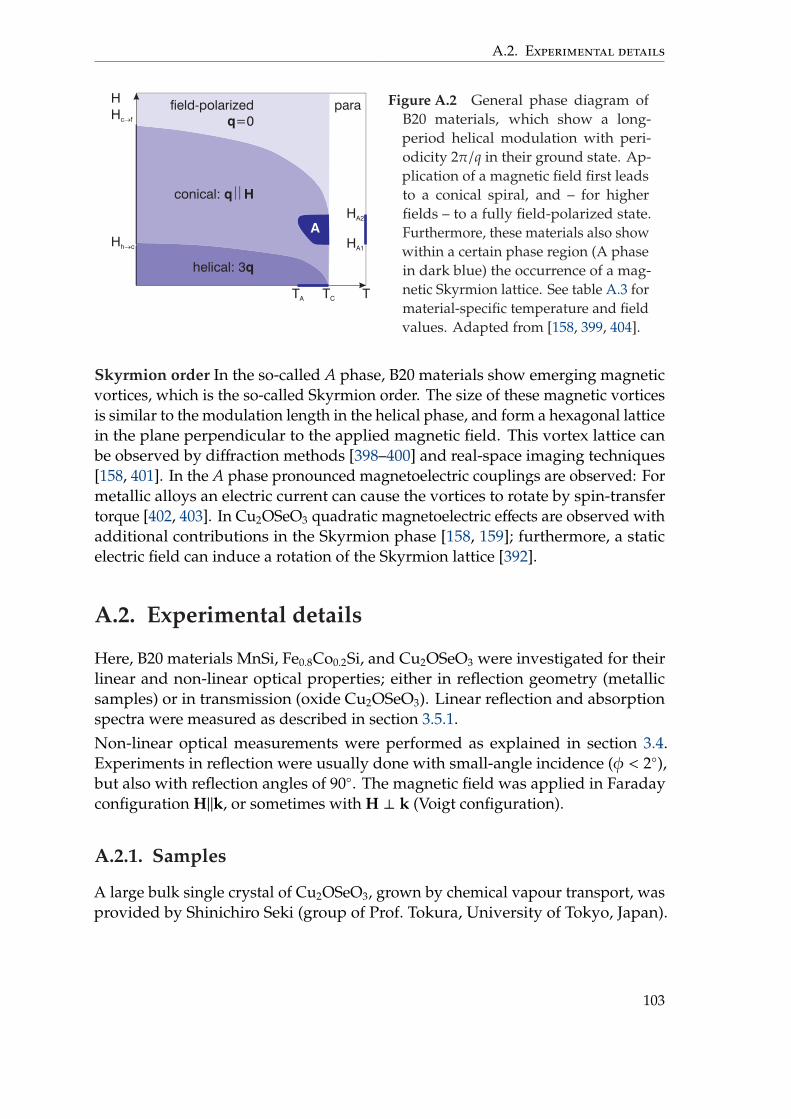
A.2. Experimental details
HA1
HA2
Hh®c
Hc®f
TCTA
conical: qïçH
helical: 3q
eld-polarizedq=0
A
para
T
H Figure A.2 General phase diagram ofB20 materials, which show a long-period helical modulation with peri-odicity 2π/q in their ground state. Ap-plication of a magnetic field first leadsto a conical spiral, and – for higherfields – to a fully field-polarized state.Furthermore, these materials also showwithin a certain phase region (A phasein dark blue) the occurrence of a mag-netic Skyrmion lattice. See table A.3 formaterial-specific temperature and fieldvalues. Adapted from [158, 399, 404].
Skyrmion order In the so-called A phase, B20 materials show emerging magneticvortices, which is the so-called Skyrmion order. The size of these magnetic vorticesis similar to the modulation length in the helical phase, and form a hexagonal latticein the plane perpendicular to the applied magnetic field. This vortex lattice canbe observed by diffraction methods [398–400] and real-space imaging techniques[158, 401]. In the A phase pronounced magnetoelectric couplings are observed: Formetallic alloys an electric current can cause the vortices to rotate by spin-transfertorque [402, 403]. In Cu2OSeO3 quadratic magnetoelectric effects are observed withadditional contributions in the Skyrmion phase [158, 159]; furthermore, a staticelectric field can induce a rotation of the Skyrmion lattice [392].
A.2. Experimental details
Here, B20 materials MnSi, Fe0.8Co0.2Si, and Cu2OSeO3 were investigated for theirlinear and non-linear optical properties; either in reflection geometry (metallicsamples) or in transmission (oxide Cu2OSeO3). Linear reflection and absorptionspectra were measured as described in section 3.5.1.Non-linear optical measurements were performed as explained in section 3.4.Experiments in reflection were usually done with small-angle incidence (φ < 2◦),but also with reflection angles of 90◦. The magnetic field was applied in Faradayconfiguration H||k, or sometimes with H ⊥ k (Voigt configuration).
A.2.1. Samples
A large bulk single crystal of Cu2OSeO3, grown by chemical vapour transport, wasprovided by Shinichiro Seki (group of Prof. Tokura, University of Tokyo, Japan).
103

A. Optical characterization of B20 materials with Skyrmion order
Table A.3 Magnetic properties ofinvestigated B20 materials. Tem-perature and field values corre-spond to the borders of the phasediagram (in figure A.2) for bulkcrystals and magnetic field ap-plied along (110) [399, 400, 404].Neutron scattering results for qand 2π/q from [158, 405–407].
MnSi Fe0.8Co0.2Si Cu2OSeO3
q (111) (100) (100)2π/q(0 T) 180 Å 295 Å 500 Å
TC 29 K 30 K 58 KTA 28 K 23 K 56 K
HA1 100 mT 20 mT 10 mTHA2 200 mT 60 mT 35 mT
Hh→c(0 K) 100 mT 90 mT 60 mTHc→ f (0 K) 480 mT 200 mT 190 mT
For the optical experiments thin platelets with orientations (100) , (110), and (111)(typical thickness 120µm) were cut and prepared by Dirk Schemionek (TechnischeUniversität Dortmund, Germany). Polishing was done with SiO2 slurry.Polished metal samples of MnSi and Fe0.8Co0.2Si grown by floating zone techniquewith surface normals parallel to (100) and (110) were provided and prepared byAndreas Bauer (group Prof. Pfleiderer, Technische Universität München, Germany).
A.2.2. SHG selection rules
Due to the non-centrosymmetric cubic point group 231′ the investigated materialsshow strong crystallographic electric-dipole SHG with symmetry-allowed con-tributions χxyz = χyzx = χzxy. Therefore, no SHG response is allowed for k||(100).Reflecting the crystallographic symmetry SHG signals with two-fold (k||(110)) orthree-fold anisotropy (k||(111)) are expected for the other distinct “Blickrichtungen”.Detailed assignment of SHG tensors in different geometries are listed in table A.6.The major interest of this study is the investigation of unusual magnetic propertiesof B20 materials. There are several possible SH contributions coupling to magneticorder that have to be distinguished:Zero-field magnetic order The occurrence of incommensurate helical order does notbreak symmetries on a macroscopic scale, and therefore no new SHG contributionsare expected to arise below TC. But the intensity of the crystallographic SHGmay change due to changes in the linear optical properties at the magnetic phasetransition.Magnetization-induced SHG (MFISH) As the materials are non-centrosymmetric,a linear coupling between SHG response and static sample magnetization Ml(Hl) isallowed [236, 237], as discussed in section 3.2.1:
Si(2ω) = χMFISHi jkl E j(ω)Ek(ω)Ml ∝Ml(Hl)
104

A.3. Crystallographic optical properties
Figure A.4. Linear and non-linear optical spectra of Fe0.8Co0.2Si (a) and Cu2OSeO3 (b).Shown are linear absorption α or reflectivity R (solid line) measured with unpolarisedlight at room temperature, in comparison with crystallographic SHG contribution χρρz
(blue area) measured above TC. The non-linear optical spectra were normalized to theSHG signal of a silver mirror. Tuning ranges for ground and SH energy are highlightedin grey. The spectral dependence of the SHG response with the linear optical propertiesis apparent.
Magnetoelectric contributions In Cu2OSeO3 a quadratic magnetoelectric effect isallowed. In principle a coupling to the induced polarization via SHG is possible.It is distinguished from the aforementioned contribution by its field-dependence:The MFISH signal scales quadratically with the magnetisation, the magnetoelectriccontribution would scale with the fourth power.Skyrmion phase The symmetry group of the Skyrmion lattice is 6/m′mm withthe six-fold z′ axis parallel to the magnetic field H‖z′. The direction of the in-plane x′ axis is weakly determined by the magneto-crystalline anisotropy [400].Magnetically-induced electric-dipole SHG allows non-zero contributions χz′z′z′ ,χz′x′x′ = χz′y′y′ , and χx′x′z′ = χy′y′z′ , which are only observable in Voigt configurationwith k ⊥ H.
A.3. Crystallographic optical properties
As stated before, due to the non-centrosymmetry of the 23 point group, a strongnon-linear optical signal is expected and indeed observed in all investigated B20materials. The linear and non-linear properties of Fe0.8Co0.2Si and Cu2OSeO3 arecompared in figure A.4. The spectral features of their SHG response are discussedin the following paragraphs. Due to the isotropic linear optical response and theoccurrence of only one independent SHG contribution only two curves need to becompared for each material.Metallic Fe0.8Co0.2Si and MnSi In figure A.4 (a) the reflectivity and SHG spectraof χρρz are shown for the (110)-cut Fe0.8Co0.2Si-sample. The reflectivity shows ahump around 1.5 eV – however, this might be a relic of the spectrum normalization
105

A. Optical characterization of B20 materials with Skyrmion order
Anisotropies
PolariserA
nalyser0◦
90◦
A||ρ
A||z
P||ρ
P||z
P||ρz
cos·sin
2cos
3±
2cos·sin
2cos·sin
sin2
cos0
sin+
fcos
(a)C
u2 O
SeO3 ,k||(110),m
easuredin
transmission
(b)Fe
0.8 Co
0.2 Si,k||(110),m
easuredin
small-angle
reflection
FigureA
.5.A
ngular
dep
endencies
ofcrystallographic
SHG
for(a)C
u2 O
SeO3
and(b)Fe
0.8 Co
0.2 Simeasu
redabove
thetransition
temp
erature
TC ,resp
ectively.P
ointsd
enotethe
SHG
intensity,solidlines
afi
ttedm
odel(third
row)
accountingfor
thenon-linear
opticalcontributionsallow
edfor
symm
etry231′and
k||(110)as
obtainedin
tableA
.6(c).
Diagram
sin
(a)and(b)have
thesam
escale,unless
notedotherw
ise.
106

A.3. Crystallographic optical properties
top
view
in-p
lane
view
tran
sfor
mat
ion
mat
rix
SHG
cont
ribu
tion
s
(a)
k||(0
01)
( e x e y e k
) =√
2√
2
( 10
00
10
00
1
) ( e x e y e z
)0
(b)
k||(0
01)
( e + e − e k
) =1 √2
( 1i
01−
i0
00√
2
) ( e x e y e z
)0
(c)
k||(1
10)
( e ρ e z e k
) =1 √2
( 1−
10
00
11
10
) ( e x e y e z
)χ
zρρ
=χρρ
z
(d)
k||(1
11)
( e ρ e τ e k
) =1 √6
(√ 3−√
30
11−
2√
2√
2√
2
) ( e x e y e z
)χτρρ
=χρρτ
=−χτττ
(e)
k||(1
11)
( e + e − e k
) =1 √2
( 1i
01−
i0
00
1
)( e τ e ρ e k
)χ
++
+=χ−−−
=χ∗ +−−
=χ∗ −
++
Tabl
eA
.6.
Diff
eren
texp
erim
enta
lref
eren
cefr
ames
,det
erm
ined
byth
ere
lati
onbe
twee
nlig
htd
irec
tion
k(ω
),in
-pla
nelig
htfie
lds
E(ω
)&S(
2ω),
and
cubi
cdi
rect
ions
x,y,
z.Th
ela
stco
lum
ngi
ves
the
resp
ecti
veED
-SH
Gex
pect
edfo
rB2
0m
ater
ials
wit
hpo
intg
roup
231′
wit
hal
low
edco
ntri
buti
onsχ
xyz
=χ
yzx
=χ
zxy
(obt
aine
dby
appl
ying
the
tens
ortr
ansf
orm
atio
nin
equa
tion
(1.2
)).
107

A. Optical characterization of B20 materials with Skyrmion order
with regard to an aluminium mirror. The SHG spectrum shows two peaks at1.65 eV and 1.75 eV, but most of the experiments were performed at 2.1 eV wherethe non-normalised intensity of the detected signal was higher. The results fromMnSi are similar to that of Fe0.8Co0.2Si, and are therefore not shown here.Copper selenite The linear absorption spectrum of Cu2OSeO3 in figure A.4 (b)shows only two features: a steep absorption edge at 0.95 eV, and a transparencywindow centred around 2.2 eV (560 nm), leading to the deep green colour of thethin platelet samples. Apart from this, no other optical anomalies were found, inagreement with other studies [408]. The strong absorption is most likely linked toseveral metal-oxygen charge transfer transitions.The tuning range for the SHG experiments was chosen to cover the charge-transferedge and the transparent region around 2.2 eV as most likely frequency combinationfor a strong non-linear optical response. As shown in figure A.4 (b), a SHG doublepeak signal was detected at 2.1 eV and 2.2 eV and a smaller response around 1.85 eV.Crystallographic SHG in B20 materials As stated before, the crystallographicSHG signal is strong due to the breaking of the inversion symmetry. In fact,the crystallographic SHG signal can be used to orient the in-plane axes even atroom temperature. Both in metallic and insulating samples only the allowedcrystallographic tensor components are observed. Their angular dependencies asshown in figure A.5 can be fully described by the symmetry selection rules forpoint group 231′. No surface SHG was detected for the metallic samples, even ifthe experiment was performed with large reflection angles.Although symmetry selection rules predict no response from a (100)-cut sample,a small response was always detected in this geometry, independent of the in-vestigated material. This could be related to a minor misalignment. But even atroom temperature – where sample rotation and tilt are much easier to control – aresidual signal was always measured, which could point to a different mechanismof two-photon fluorescence [214].In conclusion, the crystallographic SHG response of both metallic and insulatingB20 materials is determined by the non-centrosymmetric point group and the linearoptical properties.
A.4. Magnetic SHG
The main point of the present study was to identify non-linear optical signalscoupling to the helical and Skyrmion magnetic structure in the B20 materials.Therefore, experiments at low temperature and with applied magnetic and electricfields were performed.B20 alloys MnSi and Fe0.8Co0.2Si No new non-linear tensor contributions indicating
108

A.4. Magnetic SHG
Figure A.7. Magnetic SHG in Cu2OSeO3. All experiments were performed on (110)-cutplatelet of Cu2OSeO3 with the magnetic field applied in beam direction H||k||(110).(a) Normalized SHG spectra of all susceptibility contributions at zero field and 1 Tat 56 K. Symmetry selection rules and magnetic-field dependence can be used toassign crystallographic and MFISH contributions. (b) Temperature-dependence ofχρρρ(2.19 eV) ∝M. (c) Magnetic field sweeps of χρρρ(2.19 eV) at different temperatures.Changes in the curve’s slope indicate the saturation magnetization. In this experiment,also an electric field was applied. No anomaly related to the Skyrmion phase (shadedregion) is seen. The asymmetry of the curve is probably due to some minor misalignmentsof the sample. Sweeps were done from negative to positive fields.
a loss of point group symmetry were observed in any of the four metallic samples.Although the linear reflectivity is expected to change with the onset of magneticorder [409, 410], no reproducible temperature dependencies of SHG could bemeasured. One problem to consider is the effect of laser heating: In comparisonwith the laser properties used in [411] the sample temperature in the current SHGexperiments was expected to be in quasi-equilibrium, so that the magnetic phaseshould have been entered here at least at lower temperatures. Still, no signalcoupling to the magnetic order has been found in temperature- or magnetic-field-dependent measurements.Insulating Cu2OSeO3 Since no signatures of the long-period magnetic phasesin metallic MnSi and Fe0.8Co0.2Si had been found, further experiments focussedon oxide Cu2OSeO3. As in the case of the metallic samples no new SHG contri-butions were observed after zero-field cooling into the magnetic phase. This isin agreement with other studies failing to find evidence for a lowering of pointgroup symmetry at the magnetic transition [397, 412]. SHG signals coupling tothe sample magnetization were found, however: Figure A.7 (a) shows the spectraldependence of all non-linear contributions in configuration H||k||(110) and 56 K at
109
A. Optical characterization of B20 materials with Skyrmion order
zero field (grey) and 1 T (blue). Crystallographic contributions χzρρ = χρρz are onlyweakly dependent on field or temperature, whereas contributions χρzz, χρρρ, andχzρz couple linearly to the sample magnetization M(H). χzzz vanishes, in agreementwith symmetry selection rules for magnetization-induced SHG (see table 3.2). Thetemperature-dependence of χρρρ(200 mT) in figure A.7 (b) shows the behaviour ofthe field-induced magnetization and the magnetic transition around 56 K [396].As magnetic Skyrmion order and related magnetoelectric effects are expected ina limited phase space below the transition temperature TC ≈ 58 K, various field-cooling and magnetic field sweep experiments were performed in both Faradayand Voigt geometry, however no additional SHG signal was found. The mostpromising experiment looked for features in combined electric and magnetic fieldsas shown in figure A.7 (c). Here, an electric field E(111) of 165(5) V/mm was appliedwhile sweeping the magnetic field H110 at different temperatures.1 At increasingtemperature, both SH intensity and saturation field – as indicated by the kink inthe curve – decrease when approaching the transition temperature. Above TC onlya small signal, probably related to the paramagnetic magnetization, is observed.No anomalies in the field range 20 mT to 60 mT are observed, however, thus againshowing that SHG is proportional to the net magnetization only and does notcouple to helical or Skyrmion magnetic structures or the related magnetoelectriceffects.Circular dichroism in Cu2OSeO3 As the B20 space group P213 is chiral, circulardichroism – that is different absorption for σ+ and σ− light – is to be expected. It wasindeed observed in (100)-cut samples: Large transmission coefficients for infraredlight with “minus” polarization σ− contrasts with a strong absorption for “plus”light σ+, e.g. at 0.9 eV transmission coefficients are 85% and 60% for σ− and σ+ light,respectively.Below the magnetic phase transition, the difference of transmission τ− − τ+ seemsto decrease with decreasing temperature (at 0.83 eV). This might indicate that themagnetic and crystallographic handedness have different sign. Also a peculiarbehaviour with applied magnetic field H||k is observed: A negative field H < 0has no effect on the linear optical properties, whereas for H > 0 the transmissiondifference (τ− − τ+) was reduced. This effect seemed to be proportional to thesample magnetization, as the field-dependent curves show a slight kink where themagnetization is supposed to saturate.SHG spectroscopy revealed that only incident σ− light induces a non-linear responseon (100)-cut samples, whereas no (or only a very small) signal was observed for σ+
light. Since no SHG signal should be allowed in this particular configuration, these
1The electric field was chosen to point in a general direction as different magnetoelectric effectsrelated to the Skyrmion phase are expected for applied fields along both the space diagonal (111)as well as along the face diagonal (110) (see [392] and [159], respectively).
110
A.5. Conclusions
observations might indicate that two-photon fluorescence might also play a role inthe non-linear optical response in Cu2OSeO3.While this study was not very systematic, the results clearly show that crystaland magnetic chirality play an important role in Cu2OSeO3, as already known formetallic B20 alloys. These materials are found to be enantimorph-pure [385–387],but the dominance of one crystal handedness of Cu2OSeO3 it is not exactly clearfrom the literature. The optical spectra suggest that one chirality dominates overlarge crystal volumes of 0.1 mm3 and larger.Although not measured, the observation of circular dichroism can also be expectedfor incident light along the three-fold axes of Cu2OSeO3 (k||(111)).
A.5. Conclusions
In summary the observed non-linear optical properties of the B20 materials aremostly determined by the lack of an inversion centre in the crystallographicstructure and their linear optical properties. No evidence for a lowering of pointgroup symmetry in the magnetic phases – including the Skyrmion phase – wasfound. Especially, reproducible results were not obtained for magnetic phases inmetallic MnSi and Fe0.8Co0.2Si, where laser heating might have been a problem.In Cu2OSeO3 SHG contributions coupling to the net magnetization were identified(MFISH), as allowed by non-centrosymmetric crystal symmetry. No particularsignatures of phase transitions between helical, conical, and Skyrmion phase weredetected, however.The optical circular dichroism and its relationship to crystallographic and magneticchirality might be worth an additional study. Another route to investigate specifi-cally the chiral symmetry of a Skyrmion vortex lattice is to employ other non-linearoptical techniques like sum or difference frequency generation [228, 229].2
2In contrast to SHG, SFG or DFG allow coupling to chiral contributions of the non-linear tensor.“Chiral” second-order processes involve terms χi jk = −χik j which vanish for SHG due to theintrinsic tensor symmetry.
111

B. Magnetically induced phasematching in MnWO4
While phase matching is a well-known technique to enhance the non-linear response, it usually is only considered in transparent non-centro-symmetric materials. In this chapter the continuous energy shift acrossthe visible spectral range in ruby-coloured centrosymmetric MnWO4 ispresented. In this material, the second harmonic response is enabledby the magnetically induced inversion-symmetry breaking, and due tothe linear optical properties (refraction and absorption) its response isgreatly enhanced by phase matching.
The process of optical second harmonic generation (SHG) describes the simultane-ous absorption of two photons with the same energy and a re-emission of a photonwith twice the initial energy [218]. This is a virtual process not involving occupancyof real intermediate electronic states, however, like all other physical processes itmust obey the general conservation laws.The preservation of energy is clearly accounted for by the equation 2~ω = ~ω + ~ω.On the other hand, the momentum mismatch
∆k = k(2ω) − 2k(ω) (B.1)
as already introduced in section 3.3 and figure 3.3 (c) depends strongly on thedirection and polarisation of the light fields E(ω), S(2ω) with respect to the opticalproperties given by the refractive indices of the investigated material.In other words, equation (B.1) describes how much incident and generated lightfield stay in phase during the passage through a crystal – if it is fulfilled, the SHGintensity is greatly enhanced, as no destructive interference occurs and signal isgenerated across the whole optical path. On the other hand, a non-zero momentummismatch reduces conversion efficiency.For negligible absorption at both ω and 2ω the momentum mismatch in equa-tion (B.1) vanishes if the so-called phase-matching condition is met:
n(2ω,S) = n(ω,E) , (B.2)
with n(E(ω)) and n(S(2ω)) denoting the respective optical refractive indices, whichdepend on both energy and polarisation of the light fields. Therefore, linear
113

B. Magnetically induced phase matching inMnWO4
Figure B.1 Relevant directions inthe MnWO4 phase matching exper-iment: (a) Top view of the incidentand SH light field E(ω) and Sy(2ω)with respect to the surface normaln parallel to the magnetic easy axise.a. If the sample is rotated by φaround the polar axis b the incidentbeam is refracted, and the propaga-tion direction within the sample isk′. (b) Relationship between sam-ple, crystallographic, and opticalframes of reference: The sample ro-tation φ = ∠(k,n) is given withrespect to the surface normal n,which lies in the crystallographicac-plane. The axes Y, Z of theoptical indicatrix ellipse n(E) areconfined to lie in the same planeat an inclined angle. Using equa-tions (B.3) and (B.4) the directionk′ of the refracted beam can be cal-culated.
dispersion is of great importance for the non-linear conversion efficiency. If thecondition in equation (B.2) is met, the SHG signal is expected to be sensitive tochanges of frequency ω or angle of the incident light (so-called walk-off, e.g. dueto misalignment or finite beam divergence) as well as external parameters likesample temperature [210, 264, 265]. In certain cases, periodically poled ferroelectricmaterials enable that E(ω) and S(2ω) stay in phase throughout the crystal, leadingto a coherent enhancement of the SHG intensity. This technique is called quasi-phasematching [413–417].Non-linear crystals employed for frequency converters usually are transparent,non-centrosymmetric materials, which exhibit both high non-linear coefficientsand suitable optical dispersion. Here, we report magnetically induced SHG phasematching over the whole visible spectral range in coloured, centrosymmetricspin-spiral multiferroic MnWO4.
114

B.1. Experimental details
B.1. Experimental details
MnWO4 crystallises in the centrosymmetric space group P2/c1′ with two-foldsymmetry axis b and a monoclinic angle β = ∠(a, c) = 91.1◦ only deviating slightlyfrom a square angle [331]. Thin platelets of samples have a ruby-red colourinduced by charge-transfer and crystal-field transitions of the Mn2+ ions. Due tothe monoclinic symmetry optical birefringence is observed, and the material isconfirmed to be biaxial positive [346].At low temperatures (7 K to 12 K) the magnetic order indices a finite spontaneouspolarisation of 50µC/m2 [178, 333]. In this non-centrosymmetric phase a non-zeroSHG response was found [252, 351], which could be used to image the multiferroicdomains [350, 352]. Although the spontaneous polarisation enabled by the breakingof inversion symmetry due to the magnetic order is rather small compared to thatof conventional ferroelectric materials, the non-linear optical conversion efficiencyin MnWO4 is relatively high [254].Here, the spectral dependence of the SHG response of MnWO4 for different anglesof incidence was investigated using a transmission setup described in section 3.4.As light source an optical parametrical oscillator (OPO) pumped by a Nd:YAGlaser (pulse width 7 ns) was used, which allows the incident energy ~ω to be tunedfrom 0.5 eV to 1.5 eV. The experiments were performed at 7 K where both theferroelectric polarisation of MnWO4 and the related SHG signal is maximal.The geometry of the experiment is shown in figure B.1 (a): The ground wave ishorizontally polarised, while the polarisation of the SH wave is vertical and parallelto the rotation axis. The sample was rotated about the b axis, changing the incidentlight polarisation between a and c. According to equation (B.2) the phase matchingcondition is thus met at different energies, leading to a spectral shift.The surface normal n of the sample was chosen to be parallel to the magnetic easyaxis e.a., which lies in the ac plane at an angle of ∠(a, e.a.) = 33.9◦. Figure B.1 (b)shows the relationship between the three relevant coordinate systems – the sampleframe, the crystallographic directions a, b, c, and the axes of the indicatrix ellipsoidX, Y, Z. The latter is used to determine the index of refraction n(ω,φ) for theincident light field E(ω,φ) in order to calculate the direction k′(ω) of the groundwave within the sample.
B.2. Phase-matched SHG in MnWO4
Figure B.2 shows the energy dependence of the SHG intensity for different anglesφ′ between the surface normal and light direction k′(ω) within the crystal: Fornormal incidence, the SHG signal peaks at 2.31 eV while the central energy showsa blue shift (red shift) at positive (negative) sample rotation angles φ.
115

B. Magnetically induced phase matching inMnWO4
Figure B.2. SHG peak shift with the sample rotation in MnWO4: Here, the second-harmonic spectra are shown with varying (internal) direction ∠(k′, a) of the incidentlight field E(ω,φ). Line colours correspond to the wavelength of the SHG peaks. Centralenergy and peak width are indicated by the bars below the curves. End cases χbaa at1.96 eV and χbcc at 2.75 eV taken from [252]. The dashed grey line corresponds to theprediction of phase matching angles based on equation (B.2) and interpolation of therefractive indices [346].
As indicated by the colours of the peaks, and the central energies marked by theerror bars the SH signal covers a wide spectral range from red to blue. Includingthe end cases χbaa and χbcc from [252] the covered wavelength range reaches from450 nm to 630 nm.The different curves were fitted with a Lorentzian peak function, and the fit resultsare listed in table B.3, together with the sample rotation angle φ and the directionof propagation within the crystal given by φ′.Calculation of refraction angle φ′ Although the propagation of light in an opticallybiaxial material is not trivial [418, 419], the angle of refraction within the materialcan be determined knowing the sample rotation angle φ and the energy of theincident light (which equals to half of the SH central energy 2~ωc):First, the refractive index n for E(ω,φ) must be calculated. As shown in figure B.1 (b)the angle φ also determines the polarisation direction with respect to the in-planeaxes Y, Z of the optical indicatrix. The frequency dependence ni(ω) of the mainrefractive indices nX < nY < nZ can be expressed by a Sellmeyer equation withmaterial parameters given in [346]. The refractive index n(ωc, φ) is then given byan ellipse equation, with relative angle θ = ∠(Y,E) = 90◦ − φ − ∠(Y, e.a.).
1n2(φ,ω)
=cos2 θ
n2Y(ωc)
+sin2 θ
n2Z(ωc)
, (B.3)
Second, the incident and refracted angles φ and φ′ with respect to the surfacenormal are connected via the Descartes-Snellius relationship [420]:
tan(φ′) =sin(φ)√
n2(ωc, φ) − sin2(φ). (B.4)
116

B.2. Phase-matched SHG inMnWO4
φ ∠(k′, a) ~ωc ~w Aext. int. (eV) (eV)
91.1◦ 1.958 0.041−40◦ 50.5◦ 2.108 0.035 19 480−30◦ 46.6◦ 2.148 0.033 33 752−20◦ 42.6◦ 2.201 0.028 37 757−10◦ 38.3◦ 2.249 0.027 28 987
0◦ 33.9◦ 2.307 0.024 19 67610◦ 29.5◦ 2.351 0.022 780020◦ 25.1◦ 2.393 0.010 197430◦ 21.0◦ 2.446 0.006 159040◦ 17.1◦ 2.494 0.007 578650◦ 13.6◦ 2.522 0.008 11 42660◦ 10.7◦ 2.573 0.009 12 57870◦ 8.5◦ 2.603 0.011 652480◦ 7.2◦ 2.629 0.021 3274
0.0◦ 2.751 0.033
Table B.3 Details of the phasematched signals presented in fig-ure B.2: The different peaks werefitted with Lorentz functions
ISHG(ω) =2Aπ
w(ω − ωc)2 + w2 .
The obtained central frequency ω,width w, and area A are listed inthe right three columns. Internal di-rection ∠(k′, a) was calculated fromthe rotation angle φ = ∠(k, e.a.) andcentral frequency ωc using equa-tions (B.3) and (B.4).
While the investigated rotation angle φ of the sample lies between −40◦ and 80◦, thepropagation direction of the ground wave within the material lies between 7◦ and51◦ with respect to the crystallographic a axis (see table B.3). As shown in figure B.2for these directions an almost linear energy shift 0.118 eV/10◦ with φ′ is observed.Phase matching condition From equation (B.2) and the refractive indices given in[346] the phase matching angle and optimum energy can be calculated. In figure B.2this prediction is marked by a grey dashed line:1 At lower energies the theoreticaland experimental values coincide rather well2 while at higher energies the modelbased on equation (B.2) loses validity.This deviation between theoretical prediction and experimental observation islinked to the non-transparent properties of MnWO4 – at higher photon energies therefractive index nX(2ω) of the SHG wave can neither be extrapolated not directlymeasured any longer. From the continuous shift of the SH peak energy it can eitherbe concluded that nX(2ω) is larger than its value calculated from the Sellmeyerequations [346] and the strong dispersion leads to anomalous phase matching [422].Energy dependence of the conversion efficiency Finite optical absorption also hasa profound effect on the magnitude of the SHG signal, as shown in figure B.4 (a):Here, the SHG intensity dependent of the peak energy (circles) is shown incomparison with the linear absorption coefficient α at 2~ω (orange line).
1Values calculated by Petra Becker-Bohatý, University of Cologne, Germany.2Angular deviations of a few degrees are considered normal in such calculations [421].
117
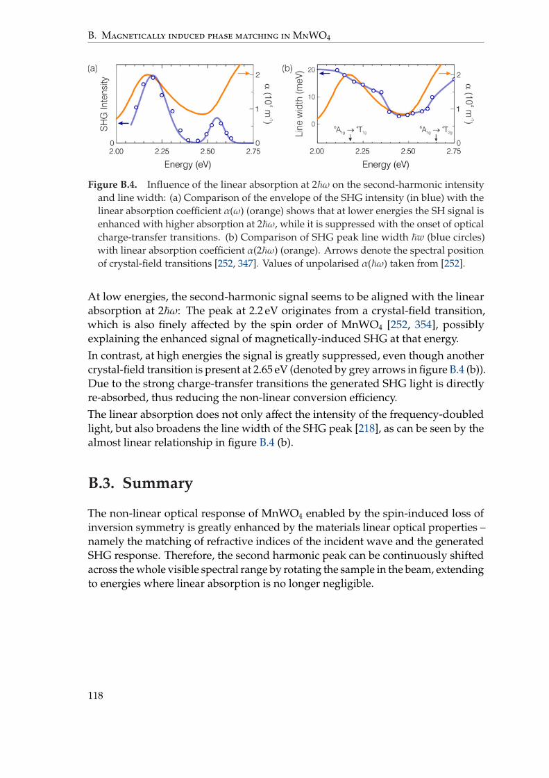
B. Magnetically induced phase matching inMnWO4
Figure B.4. Influence of the linear absorption at 2~ω on the second-harmonic intensityand line width: (a) Comparison of the envelope of the SHG intensity (in blue) with thelinear absorption coefficient α(ω) (orange) shows that at lower energies the SH signal isenhanced with higher absorption at 2~ω, while it is suppressed with the onset of opticalcharge-transfer transitions. (b) Comparison of SHG peak line width ~w (blue circles)with linear absorption coefficient α(2~ω) (orange). Arrows denote the spectral positionof crystal-field transitions [252, 347]. Values of unpolarised α(~ω) taken from [252].
At low energies, the second-harmonic signal seems to be aligned with the linearabsorption at 2~ω: The peak at 2.2 eV originates from a crystal-field transition,which is also finely affected by the spin order of MnWO4 [252, 354], possiblyexplaining the enhanced signal of magnetically-induced SHG at that energy.In contrast, at high energies the signal is greatly suppressed, even though anothercrystal-field transition is present at 2.65 eV (denoted by grey arrows in figure B.4 (b)).Due to the strong charge-transfer transitions the generated SHG light is directlyre-absorbed, thus reducing the non-linear conversion efficiency.The linear absorption does not only affect the intensity of the frequency-doubledlight, but also broadens the line width of the SHG peak [218], as can be seen by thealmost linear relationship in figure B.4 (b).
B.3. Summary
The non-linear optical response of MnWO4 enabled by the spin-induced loss ofinversion symmetry is greatly enhanced by the materials linear optical properties –namely the matching of refractive indices of the incident wave and the generatedSHG response. Therefore, the second harmonic peak can be continuously shiftedacross the whole visible spectral range by rotating the sample in the beam, extendingto energies where linear absorption is no longer negligible.
118

C. Domain image analysis
The spatial anisotropy of ferroic domains is determined by internalinteractions and defects, as well as external influences like thermaltreatment and applied fields. The comparative analysis of shape, size,and distribution of mesoscopic domains can therefore give insight tounderlying physical effects on a micro- or macro-scale.Here, a series of images of ferroelectric domains growing in an electricfield is analysed automatically. The following chapter tries to give abrief tutorial-like introduction into the use of MatLab to investigate suchimage sequences.
Ferroic domains are volumes with uniform alignment of the microscopic orderparameter, and often have sizes in the micro- or nano-meter range. The shape, size,and distribution of these domains reflect the underlying microscopic mechanisms,and strongly affect macroscopic properties. In particular, the dynamic responses toapplied fields like material susceptibilities and switching processes are governedby domain growth and domain wall motion.The spatial anisotropy of a mesoscopic domain pattern generally minimizes theglobal energy (and entropy) by spatially modulating the order parameter. As aconsequence of competing energies related to uniform volumes and boundariesseparating them, different domain morphologies like bubble-, stripe-, or maze-likepatterns can emerge [289, 378, 423].The shape of ferroelectric domains is often heavily influenced by electrostaticrepulsion and strain matching, whereas the distribution of ferromagnetic domainsis mostly governed by stray fields and the spatial anisotropy of the exchangeinteractions [18, 34, 35]. With applied fields the growth of domains is often foundto be highly anisotropic, too.Therefore, the analysis of static (equilibrium) and dynamic domain patterns cancharacterise the observed structures and reveal some indirect insight into theunderlying microscopic interactions. To get comparative and reproducible resultsfor even a large number of images, it is advisable to analyse the domain images ina systematic and automatised way. Using a computer-assisted study also has theadvantage of being fast (once scripted and optimised), reproducible, and adaptableto other cases.
119

C. Domain image analysis
Figure C.1 Interesting parameters of adomain pattern: (a) From a singleimage, areas and boundaries can beextracted. The comparison of subse-quent images allows to quantify dy-namic properties as area change andforwards velocity. Especially inter-esting are cross-correlations betweenthese properties. (b) Point-to-pointdisplacement ∆y and angle φ are de-termined by the boundary shape andthe chosen correlation length L.
This chapter is intended to be used as a tutorial to guide such an analysis andis structured as follows: First, the general concepts of domain pattern and theircharacterisation are briefly discussed. The second section describes the MatLabscripts and functions used to analyse an image sequence of ferroelectric domainsin Mn0.95Co0.05WO4. In the end, the results of this study are discussed.
C.1. Properties of domain patterns
An image showing ferroic domains is always a projection of the three-dimensionaldomain topography of the sample. Depending on the experimental techniqueused to image domain patterns typical resolutions range from the millimetre tothe nanometre scale [34, 35, 424]. Domain images typically show different areaswhich are separated by curves tracking the position of the domain boundaries. Itis noteworthy that in many cases the resolution limit is larger than the physicalwidth of the domain wall, and therefore the boundaries usually appear broaderthan they actually are.The analysis of domain pictures can either focus on the different areas or on theboundaries between them, as schematically illustrated in figure C.1 (a). In the firstcase, the distribution of domains can be analysed with regard to typical sizes andshapes, their distribution, and – if a contrast is present – the balance of differentdomain states and their connectivity [328, 425]. In the second case, the boundariesseparating different domains can be characterised by their preferred direction,typical curvature, or roughness. Also dynamic features, like forward motion orarea change, can be investigated if the imaging method is fast enough to trackcontinuous changes in the domain distribution. Especially interesting are thecross-correlations between all these properties.The main focus of the following analysis was on the anisotropy and roughness ofthe boundaries during the field-driven domain growth. Therefore in the following
120

C.2. Computational details
paragraphs the autocorrelation functions measuring statistical displacements anddirection are defined.As shown in figure C.1 (b) the difference between two points of the domain boundaryis given by the horizontal distance L and the vertical displacement ∆y. Averagingthe square of this displacement for the whole curve and a given autocorrelationlength L defines the correlation function B(L) [426]:
B(L) = (y(x) − y(x + L))2 ∝ L2ζ . (C.1)
As indicated in the above equation, the dependence of B(L) on L is expected tofollow a power law, and the exponent ζ depends on the dimensionality of thesystem and the underlying pinning potential [65, 426].Another way to quantify the local deviation of a boundary from a straight line isto calculate the angle between two points separated by L, which again defines anautocorrelation function:
φ(L) = arctan(∆yL
). (C.2)
The average of the angle φ(L) indicates the general inclination or slope of thecurve. Furthermore, the norm of the angle is closely related to the boundaryroughness
√B(L), as |φ(L)| gives an estimate how much the curve meanders around
the horizontal straight line.
C.2. Computational details
The following part of this chapter deals with the analysis of an image sequenceshowing an electric-field-driven growth of ferroelectric domains in Mn0.95Co0.05WO4.The experiment is described in section 5.5.3, and the full set of eighty-four images,each taken every six seconds, can be seen in figure C.2: After starting from a single-domain state (upper left image), indicated by uniform brightness, the applicationof a constant electric field first leads to nucleation and then to continuous growth ofdomains with opposite polarity, ending with two domains of approximately equalarea (bottom right image).The goal of the computational analysis of these images was to automaticallydetermine the domain area and the boundary curve, as well as to calculate theautocorrelation values defined by equations (C.1) and (C.2) for these curves. Thisanalysis can be separated into three stages:
(1) Image analysis: Enhancement of images to determine areas and boundaries.(2) Curve analysis: Computation of autocorrelation values and forward velocities.(3) Data exploration: Reduction of data complexity by calculating statistics,
visualising results and searching for cross-correlations.
121

C. Domain image analysis
Figure C.2. Growth of ferroelectric domains in a constant electric field in Mn0.95Co0.05WO4.The horizontal axis is parallel to the polar b direction. The SHG images were taken everysix seconds, and the shown sequence of 84 images took about eight minutes to record.Further details about the experiment can be found in section 5.5.3 and figure 5.5.
122

C.2. Computational details
Continuation of figure C.2. Growth of ferroelectric domains in a constant electric field inMn0.95Co0.05WO4. The horizontal axis is parallel to the polar b direction. The imageswere taken every six seconds, so that the shown sequence of 84 images took about eightminutes to record. Further details about the experiment can be found in and .
123
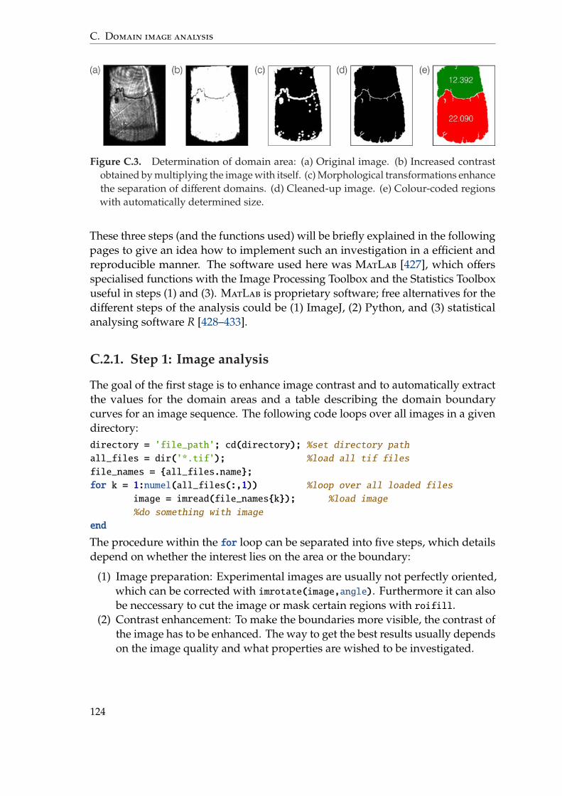
C. Domain image analysis
Figure C.3. Determination of domain area: (a) Original image. (b) Increased contrastobtained by multiplying the image with itself. (c) Morphological transformations enhancethe separation of different domains. (d) Cleaned-up image. (e) Colour-coded regionswith automatically determined size.
These three steps (and the functions used) will be briefly explained in the followingpages to give an idea how to implement such an investigation in a efficient andreproducible manner. The software used here was MatLab [427], which offersspecialised functions with the Image Processing Toolbox and the Statistics Toolboxuseful in steps (1) and (3). MatLab is proprietary software; free alternatives for thedifferent steps of the analysis could be (1) ImageJ, (2) Python, and (3) statisticalanalysing software R [428–433].
C.2.1. Step 1: Image analysis
The goal of the first stage is to enhance image contrast and to automatically extractthe values for the domain areas and a table describing the domain boundarycurves for an image sequence. The following code loops over all images in a givendirectory:directory = ’file_path’; cd(directory); %set directory pathall_files = dir(’*.tif’); %load all tif files
file_names = {all_files.name};for k = 1:numel(all_files(:,1)) %loop over all loaded files
image = imread(file_names{k}); %load image
%do something with image
end
The procedure within the for loop can be separated into five steps, which detailsdepend on whether the interest lies on the area or the boundary:
(1) Image preparation: Experimental images are usually not perfectly oriented,which can be corrected with imrotate(image,angle). Furthermore it can alsobe neccessary to cut the image or mask certain regions with roifill.
(2) Contrast enhancement: To make the boundaries more visible, the contrast ofthe image has to be enhanced. The way to get the best results usually dependson the image quality and what properties are wished to be investigated.
124

C.2. Computational details
Figure C.4. Determination of domain boundary curve: (a) Original image. Subtraction ofa blurred version of this image (b) enhances the domain boundaries (c). Clean-up of theblack-and-white image (d) allows to extract the domain boundary curves (d). For thesubsequent analysis only the lower half of the longest (blue) curve was used.
(3) Conversion to black-and-white image: im2bw(image,greythresh(image)) con-verts the grey-scale image to binary mode, with automatically determinedthreshold.
(4) Clean-up and fine-tuning: The reason for using black-and-white images isthat many morphological operators are available to manipulate and enhancestructural features (see chapter 16 of [434]). MatLab functions worth mention-ing here are bwareaopen(image,n) and bwmorph(image,mode): The first removesall white areas containing less than n pixels, whereas the second appliesdifferent morphological transformations depending on the chosen mode.Sometimes these operations have to be combined with imcomplement(image),which reverses black and white pixels.
(5) Recognising areas and boundaries: MatLab offers several functions auto-matically recognising properties of areas and boundaries. The success ofthese operations depend on the diagonal un-connectedness of the different(white) areas, so bwmorph(image,’diag’) should be used before. After savingthe results one can continue with the second step of the analysis.
Figure C.3 illustrates the different steps in extracting the domain areas: After theimage was rotated (a), the contrast between domains is enhanced by multiplyingthe image with itself using immultiply(image,immultiply(image,f)) (the optimalvalue for the exponent 1+ f has to be determined by hand). In (b) the contours weresharpened with imsharpen(image), then image was transformed to binary mode (c).Since the main boundary separating the two areas was not a continuous line, theconnectivity was enforced by several bwmorph transformations with the options’thicken’ and ’bridge’. As can be seen by comparing (a) and (d) these operationsdo not fully preserve the domain shape. Even with this systematic error the analysisof a full image sequence sill should give the right trends and comparable results.The values for the areas can be extracted using stats=regionprops(image,’Area’),and transpose([stats.Areas]) gives a table with the results. To produce an imagewith coloured regions as in figure C.3 (e) refer to the functions labelmatrix andlabel2rgb.
125

C. Domain image analysis
The determination of the domain wall curves is illustrated in figure C.4: A niftytrick to extract only the inner curves shown in (c) (and e.g. not the sample boundary)is to subtract the blurred image (b) from itself (a):1
imadd(immultiply(image,2),imcomplement(medfilt2(image,[30,30])));
The best results are achieved using a median blur (instead of a Gaussian filter), anda large filtering area. imadjust(image) further enhance the contrast.To calculate correct values for the properties of the domain wall and its forwardvelocity, the shape of the boundary curve should be as exact as possible with respectto the original image. Using bwmorph with the options ’spur’, ’thin’ and ’diag’(in that order) will produce the result shown in figure C.4 (d). The edges of thewhite areas are recognised using [table]=imcontour(image,1). This table has tobe transposed (transpose(table)) and the different parts of the contour can beseparated by finding points that have large separation. The result is visualised infigure C.4 (e). In the end, only the upper part of the longest curve was saved withdlmwrite(filename,table) for the subsequent analysis, with the file name given bythat of the original picture file, containing the time stamp when the image wastaken.
C.2.2. Step 2: Curve analysis
Once the domain boundary curves were obtained, their properties can be computedin a rather straight-forward way. The static autocorrelation values of B(L), φ(L),and |φ(L)| are calculated using equations (C.1) and (C.2) for all point pairs withdistances from 1 px to 50 px corresponding to 6µm to 300µm.To characterise the forward motion, first points with the same x value have tobe determined in subsequent images. Dividing the vertical displacement by thetime difference gives the forward velocity v = ∆y/∆t. The time between images isapproximately six seconds, and can also be extracted from the time stamp in thefile name with the following code:pattern = ’[0-9]{6,6}\.[0-9]{3,3}’; %timestamp pattern
timestamp = regexp(name, pattern, ’match’); %timestamp as string
timeFormat = ’HHMMSS.FFF’; %timestamp format
time = 24*60*60*datenum(timestamp,timeFormat); %time in seconds
It makes sense to write MatLab functions for the different small routines, whichmakes it easier to reuse and adapt them. Additionally the main code is shorter andeasier to understand, which is helpful when problems occur.All the results were stored in an ASCII table. The reason not to store only averagedvalues is that certain cross-correlations between variables might not be detected inan abridged data set.
1Thanks to Chris Wetli for sharing!
126

C.2. Computational details
Domain textures can similarly be analysed using the concepts explained in [434]and the MatLab functions graycomatrix and graycoprops.
C.2.3. Step 3: Data exploration
The best way to access the calculated results in MatLab is to store them in a dataset,which is part of the Statistical Toolbox. It allows easy handling of large arrays of data,and to sort, filter, analyse, and visualise them. To convert an ASCII table to a dataset,first the file is loaded using table=importdata(filename); and then converted withd = mat2dataset(table,’VarNames’,{’L’,’B’,’phi’,’v’}). The different columnsthen can be accessed e.g. by d.v. To filter the values according to a certain condition(e.g. condition = ’d.v > 0’) use d(condition,:).v.The first step in the analysis is to check, using simple statistics, if the distribution ofthe variables and the extremal values lie in the expected (and physically reasonable)range. One thing to be careful about in this step is to avoid counting invalidevents, like empty entries or that of type ’Not a Number’ (NaN). MatLab offerssome functions like nanmean(d.v) or nanstd{d.v} for calculating mean and standarddeviation of d.v automatically excluding invalid values. In other cases, they haveto be filtered out by using the syntax in the previous paragraph and functions likeisnan(d.v) and isempty(d.v).Statistics of a single variable can be characterised by several figures, like thenumber of events (size(d.v,1)), the data range given by minimal and maximalvalue (range(d.v), min(d.v), max(d.v)), mean value and its standard deviation(mean(d.v), std(d.v)), and median value and interquartile range (median(d.v),iqr(d.v)). It is note-worthy that the median and interquartile range (containingthe middle 50% of the data points) are a more robust measure of the distributionthan the mean value and its deviation, as the latter are more influenced by outliers[435]. The function boxplot{d.v,’Notch’,’on’} gives a visual summary of all theaforementioned values [436]. Histograms can be plotted with histfit(d.v) whichalso can compare the data distribution with several statistical distribution functions.An illustration of such plots is for example given for the distribution of the domainwall forward velocity in figure C.7.Cross-dependencies can be found by various means: To visualise the statisticaldistribution of the autocorrelation values of B(L), φ(L) or |φ(L)| in dependence ofthe (evenly-spaced) correlation length L, for example, a box plot is most suited(boxplot(d.B,d.L,’Notch’,’on’)). A way to picture correlations between contin-uous variables, e.g. B and φ is to use a scatter plot, like scatterhist(d.B,d.phi),which additionally shows histograms of the single-valued distributions.Non-trivial relationships, though more difficult to identify, can reveal interestingresults, such as a link between boundary roughness and forward velocity in a time
127
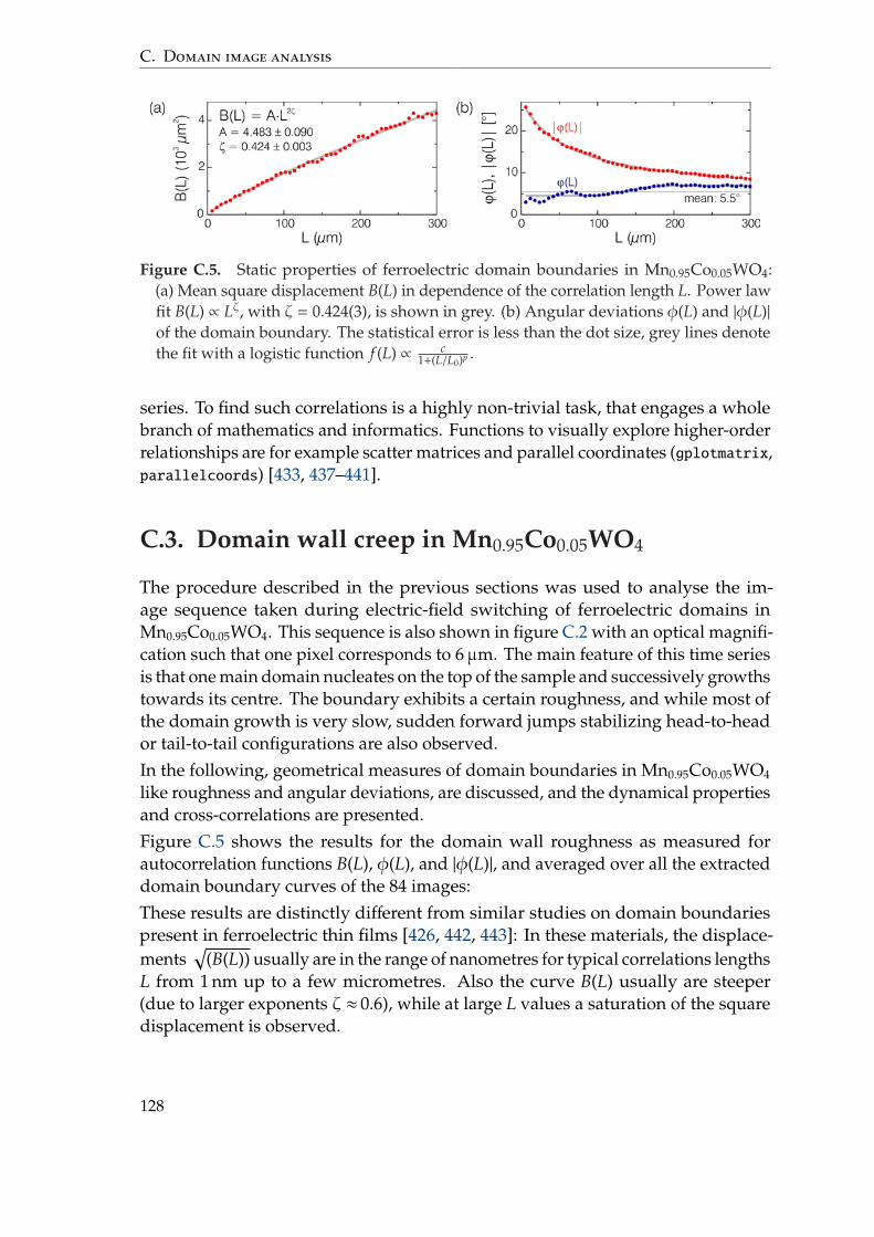
C. Domain image analysis
Figure C.5. Static properties of ferroelectric domain boundaries in Mn0.95Co0.05WO4:(a) Mean square displacement B(L) in dependence of the correlation length L. Power lawfit B(L) ∝ Lζ, with ζ = 0.424(3), is shown in grey. (b) Angular deviations φ(L) and |φ(L)|of the domain boundary. The statistical error is less than the dot size, grey lines denotethe fit with a logistic function f (L) ∝ c
1+(L/L0)p .
series. To find such correlations is a highly non-trivial task, that engages a wholebranch of mathematics and informatics. Functions to visually explore higher-orderrelationships are for example scatter matrices and parallel coordinates (gplotmatrix,parallelcoords) [433, 437–441].
C.3. Domain wall creep in Mn0.95Co0.05WO4
The procedure described in the previous sections was used to analyse the im-age sequence taken during electric-field switching of ferroelectric domains inMn0.95Co0.05WO4. This sequence is also shown in figure C.2 with an optical magnifi-cation such that one pixel corresponds to 6µm. The main feature of this time seriesis that one main domain nucleates on the top of the sample and successively growthstowards its centre. The boundary exhibits a certain roughness, and while most ofthe domain growth is very slow, sudden forward jumps stabilizing head-to-heador tail-to-tail configurations are also observed.In the following, geometrical measures of domain boundaries in Mn0.95Co0.05WO4
like roughness and angular deviations, are discussed, and the dynamical propertiesand cross-correlations are presented.Figure C.5 shows the results for the domain wall roughness as measured forautocorrelation functions B(L), φ(L), and |φ(L)|, and averaged over all the extracteddomain boundary curves of the 84 images:These results are distinctly different from similar studies on domain boundariespresent in ferroelectric thin films [426, 442, 443]: In these materials, the displace-ments
√(B(L)) usually are in the range of nanometres for typical correlations lengths
L from 1 nm up to a few micrometres. Also the curve B(L) usually are steeper(due to larger exponents ζ ≈ 0.6), while at large L values a saturation of the squaredisplacement is observed.
128

C.3. Domain wall creep inMn0.95Co0.05WO4
Figure C.6. Comparison of dynamical and boundary properties for the time series: Shown,from the bottom upwards, are the area increase (blue area), maximal forward velocity(H), averages of local angle and orientation (•, �), and the boundary roughness
√(B(L))
(�). Error bars are omitted for clarity, lines are guides to the eye.
In bulk Mn0.95Co0.05WO4 the domain boundaries exhibit a pronounced roughness√B(L)=10µm to 65µm without saturation even at high L values (Lmax=300µm), as
can be seen in figure C.5 (a). The exponent of the power law ζ=0.424(3) impliesan effective dimension of the domain wall drfd=2.7 for a random-field pinningpotential, or drbd=2.0 for random-bond disorder potential [426]. Since only onetime series (with one set of environmental variables) was investigated, a distinctionbetween these two models cannot be made.Figure C.5 (b) shows the autocorrelation values for the angles φ(L) and |φ(L)|: Thevalue of φ(L) describes the inclination of the boundary to the image horizontal.The mean value is approximately 6◦, which could be related to the angle of thenet polarisation towards the b direction [184]. In contrast, the norm value |φ(L)|gives a measure for the local deviations from a straight line, which is especiallypronounced on short correlation lengths L. Both φ(L) and |φ(L)| can be fitted usinga logistic function.Another point of interest are the dynamic properties of the switching process, bycomparing area growth, velocities, boundary roughness and angles. In figure C.6,these values were calculated for every image of the sequence: On one hand,there does not seem to be a cross-correlation of the boundary properties and theincrease of domain area. On the other hand, there is a close resemblance betweenthe roughness value
√B(150µm) and the boundary inclination φ(150µm), which
is not surprising since both values are determined by geometrical relations inequations (C.1) and (C.2).More interestingly, there seems to be a correlation between the maximal forwardvelocity vmax and the local deviation of the boundary from a straight line measuredby |φ(30µm)|.
129

C. Domain image analysis
Figure C.7 Statistical distributionof the domain boundary forwardvelocity. On the top a beeswaxplot (red scatter plot) and an expo-nential fit (in blue) of the distribu-tion are shown. The bottom dia-gram shows the summarised statis-tics in a box plot (in grey) whichmarks the interquartile range, andother values of significance. Al-though high forward velocities areobserved, too, most of the dynam-ics happens on long time scales asexpected for domain wall creep.
The calculation of the forward motion of the domain boundary lead to 11 750values, of which 16.7 % were invalid (NaN or values smaller zero). The distributionof velocities equal or larger than zero are visualised in figure C.7. The upper figureshows a beeswax plot, which is similar to a histogram. Almost sixty percent of thevalues are zero, and non-zero velocities seem to follow an exponential distribution,which is typical for a creep processes [65]. The velocity statistics are summarised ina box plot on the bottom: The rectangle marks the interquartile range (IQR) fromthe 25 % to the 75 % quantiles, whereas the whole grey part marks the range of 10 %to 90 % of the data points. Outlier ranges (1.5·IQR) are marked by black whiskers.As more than 60 % of the values are zero, the median velocity is 0µm, in agreementwith the observation that the domain boundary does not move forward betweenmost images. The mean velocity is 1.30(3)µm/s, which is consistent with the roughestimate of the velocity by the displacement between the first and last image ofthe sequence, and the time passed in between. The maximal value is 27.35µm/s,however, due to the rather bad temporal resolution of ∆t = 6 s this only gives alower margin on the maximal velocity. In summary, these values nicely describethe observed domain wall creep, interrupted by untypically large forward jumps.
C.4. Conclusions
The first part of this chapter describes interesting properties of domains and domainboundaries, and established a useful sequence for the automated analysis of domainimage sequences. These algorithms then were used to analyse the electric-fielddriven domain wall creep in multiferroic Mn0.95Co0.05WO4. The results clearlydemonstrate the overall roughness of the domain boundary even on micrometerscales and underline the slow discontinuous forward motion in the driving field.
130

C.4. Conclusions
In comparison with the results here, a study with several domain image sequencestaken at different temperatures or electric field strengths could give further insightsinto the dynamical process of multiferroic domain switching, for example whichkind of pinning is present and what the dynamical exponents are [35, 65, 426]. Withan automated image analysis these properties can be extracted in a manner that isreproducible and easy to adapt.
131


D. Sample database
With currently more than 600 scientific samples in the FERROIC researchgroup, and their numbers steadily growing, there is a need to reliablyidentify and characterize these samples. Therefore, a software with thefive following characteristics was developed: (1) An intuitive interface,(2) read and write access for every user, (3) automatic generation ofa unique sample number, (4) standardized input forms, and (5) thepossibility to upload files. Therefore, the sample database allows keeptrack of available samples even on longer time scales.
With a growing number of investigated materials and samples there is a need toreliably store information about these samples. The first attempt to standardize thedescription and subsequent numbering of new samples, was done in 2009. But asonly one person was responsible for maintaining the database, it was not widelyaccepted. Furthermore, the stored data was not standardized, and, as consequence,important pieces of information were often missing, contradictory, ambiguous,redundant, or invisible.1 As a consequence, the system was used very little and theoutput was not kept up to date.As an alternative, I developed the current sample database in 2012. It has a simpleweb interface and allows general reading and writing access. Therefore every userhas the possibility as well as the responsibility of keeping the data up to date. Thetransparent output and the possibility to upload files facilitates the quick searchingand tracking of samples.In this chapter, I first give an introduction to the functionalities of the web interfaceof the sample database, and how to use its different viewing and editing options.Then I briefly explain the software architecture and the interplay between itsdifferent parts.
1I had some problems to assign samples of RMnO3 to either the hexagonal or orthorhombic familyof rare-earth manganites. In other cases, the origin of samples was no longer known, althoughthis information is quite important, e.g. for communication and the assignment of co-authorship.
133

D. Sample database
Figure D.1 Home page ofthe sample database in-terface as of Septem-ber 2014. The leftpanel shows navigationoptions, whereas on theright the search resultsare shown. Here, on thestart page, the number ofsamples by sample type(bulk, thin film, multi-layer system etc.) aregiven.
D.1. User guide
Almost all of the sample used in the FERROIC group are grown and providedby other research groups from all over the world.2 The complete descriptionof a scientific sample – unmistakeably identified by a unique number – is thesum of many different properties, which are summarized in figure D.2. Manyattributes are directly linked to a specific sample (e.g. width, orientation, doping)while information about materials or cooperating research group can be enteredindependently into the database, and then linked to specific samples.One of the most important concepts here is the distinction between samples andsample batches: A batch describes a set of samples with common origin and sharedphysical properties: Often this means slices of varying crystallographic orientationscut from the same bulk crystal, or a thin film series with varying thickness. Asa consequence, samples in the same batch have the same sample type – likebulk crystal, thin film, multilayer systems, nano-structured meta-materials. Likeindividual samples, sample batches are uniquely identified, so that the relationshipbetween different samples within a batch is preserved, even if sub-samples arecreated.
D.1.1. Access and navigation
The database interface is available under www.samples.ferroic.mat.ethz.chfrom within the ETH intranet only. Access is restricted to members of the Ferroicgroup, and a prompt asks for netz user name and password. The start page of the
2Since recently, also by in-house fabrication by pulsed laser deposition (PLD), or floating-zone(FZ) techniques.
134

D.1. User guide
sample database looks like in figure D.1. From within the interface, the homepagecan either be accessed by selecting the menu point Overview or clicking on thegroup logo in the navigation panel on the left. On the right side, the start pageshows the numbers of samples by sample type. Clicking on an icon will lead to listof all samples within that respective category.Navigation The other three options in the navigation pane Materials, SampleUsers, and SampleGrowers lead to overview pages of the corresponding categorieswhich allow to selectively browse for samples associated to material, user, or origin.3
The forms to add new entries and edit existing ones are mostly self-explanatory andtool tips provide a short help: While the yellow light bulb explains the significanceand content of a certain input field, the blue exclamation mark provides textformatting syntax (like Greek letters, sub- and superscripts).If one looks for a specific sample with known ID, one can short-cut the search byusing the input field on the left bottom part of the navigation pane.Sample views The properties of samples are shown on the left side of the page.They can be presented in different ways – the List View gives a brief overview,while the Detailed View presents (almost) all properties and the full history ofa sample. One can toggle between those view by selecting the link "Switch todetailed/list view" in the upper right corner. A Print View with less colour andwithout the navigation panel is available, too.The Batch View can be selected from the detailed sample view by clicking the link„Show n samples in batch #xy“ under the point sample origin. It shows all samplesbelonging to a specific batch. Additionally it provides detailed information aboutsample origin, growth method, and batch history on top, with the list of samplesbelow. Batch events, which will be explained in the following section, can only beadded in this view.
D.1.2. Batch and sample history
Sample attributes (orientation, thickness, dimensions) only change if somethingis done to the sample (e.g. cutting, or lapping and polishing). Therefore, everymodification is related to some event. The button Add new event in the batch ordetailed sample view opens a form with four fields – date (in yyyy-mm-dd format),event (a drop-down menu), a text field (the user token will always be added) andthe possibility to upload a file.4 Further input may be asked for in the case ofspecific events, e.g. after lapping the thickness and dimensions of a sample will
3To find, for example, all MnWO4 samples first go to the materials page, find the material andthen select the link "Show x MnWO4 samples".
135

D. Sample database
Figure D.2. To fully characterize a scientific sample, information like that in the abovenet diagram are needed. Many of these properties can be stored independently of eachother, and later linked to a specific sample. A relational database like MySQL allows thestorage of such interdependent pieces of information, and to add constrains by format(text, number, date) and relationships.
136

D.1. User guide
have changed. Existing events can be modified, too. Files cannot be changed oncethey are uploaded, however.
D.1.3. Adding samples to the database
Before adding new samples to the database, a new batch has to be created. Thereforethis process also requires two input forms. There are a few hurdles, so the mainpoints are summarised here:Before starting Entries for the sample materials and the sample grower shouldalready exist in the database (or be added before the next steps).Add sample batch Most input fields are self-explanatory. Three information arevital for the next step: (1) The right sample type must be selected, as it determines thenumber of materials.5 (2) The number of samples in the new batch have to be given.(3) Only if the samples do not have the same material or material combination, theoption "samples all have same material - no" must be selected.Add samples The next step asks for specific information of the samples: Themeaning of most fields should be clear, but be aware that the sample descriptioncannot be changed afterwards – this field is reserved for fundamental sampleproperties only, like doping level6 or film thickness. Other characteristics likethickness, orientation, and dimensions may change and should be written down inthe corresponding fields.7
Storing samples Once the input forms are submitted, new entries for batch andsamples are created. Now it is the responsibility of the user to mark and store thesamples in a comprehensible manner. If plastic boxes are used for storage at leastthe sample ID should be written on the box. It is advisable to seal the label with apiece of Scotch tape to prevent smudging due to solvents or skin oils.8
4Portable document format (pdf) is preferred. File formats are only allowed for file extensionshaving up to four letters.
5The sample type limits the number of materials that can be selected for the sample description:Bulk single crystal (one material), thin film (one substrate plus one layer material), multilayersystem (one substrate plus up to three layer materials).
6If a sample is doped, choose the parent material, select the option "sample doped: yes", and notthe doping level in the description field. This avoids confusion due to generation of "new"materials of different doping levels.
7A set of thin film or multilayer samples often come with a substrate (most times a bulk crystal)for comparison measurements. Such a sample can also be added to a batch by choosing "samplesubstrat: yes".
8It is also a good idea to make a photo of all the samples and to annotate them with theircorresponding IDs and distinct properties. This file can be uploaded and linked with thecorresponding batch (by adding a "batch comment" to the batch history). Another way ofidentification is the use of sample aliases, which can be used together with the unique IDs.
137

D. Sample database
Figure D.3 Different layers of the sam-ple database application: The heart ofthe system is a MySQL database storingthe information. Server-sided scriptingis then used to retrieve (and write) data,and to generate a web output. The usersees the web interface only, whereas allthe data handling and presentation isdone with PHP scripts.
D.1.4. Concluding remarks
While the sample database provides a convenient framework to store informationabout scientific samples, there are some disadvantages: First, the user is not able todelete information. While this was a design choice to prevent involuntary data lossit also means that if wrong input occurred the database administrator has to deleteit manually. A second inconvenience is that sample properties can be changed onlyone-by-one. Again, the database administrator can help in that case. But the majoradvantages of the system – autonomy and transparency – should outshine theseminor drawbacks.In conclusion, discipline is still needed to keep the sample information up-to-date.
D.2. Application architecture
Before the development of the current sample database information about scientificsamples were stored in a text-based XML database: While easy maintainable andexpandable without knowing special code, the comprehensibility and completenessof sample information vastly depended on the user entering it. A survey of theold database revealed many cases with missing (often vital) information, andredundant or contradictory entries.The old system therefore served both a starting point for the development of thenew database as well as inspiration for further requirements and improvements.The main goal was to provide a system with a simple interface, read and writeaccess for every user, and forms to encourage the complete description of a sample.
D.2.1. Storing sample information
Before starting to write the first script, the format of the actual database, whichstores information about all samples, had to be decided. In contrast to the previoustext-based XML database a relational database was used. It can store data of
138

D.2. Application architecture
different tables and formats (e.g. textual, numerical, Boolean, temporal, categorical,and so on), supports auto-incrementing counters, and relational links betweendifferent entries. All these properties make such a database ideal for storinginformation with predefined and repeating structure. Here, popular open-sourceMySQL was used [444, 445].9
From the old XML database, categories and properties needed to describe ascientific sample were derived. Those attributes and their cross-relationships aresummarized in figure D.2. By separating and distributing content over severalcategories, describing their respective relationships, and restricting their format,many occurrences of data anomalies like missing, redundant, or contradictoryentries can be avoided ("database normalisation") [448–450]. Once this process wasfinished, the data from the old XML database was manually transferred to the newMySQL database.One major requirement for a new and useful sample database system was theability to upload files with further description of different samples. While MySQLalso can store files in the database, it disproportionally increases its size and slowsdown the handling of queries. So here a different approach was chosen: The filesare uploaded on the server and stored in the a folder called ./samplefiles/, and alink to the file is stored in the database.
D.2.2. Server and data handling
The MySQL database alone does not offer a usable framework, since the structureof the data must be known to access it with a specialised script language. Therefore,a web interface to access the MySQL database was developed.Several scripting languages are used in the sample database application, withserver-sided PHP10 in the centre of data handling and manipulation, as shown infigure D.3: PHP allows communication with the MySQL databases as well as thegeneration of the web output via the PHP-based template engine Smarty [451].With this separation of data handling and data presentation it is easier to maintainand update the application or interface, if needed.For the formatting of the web output HTML and CSS are used for static, andJavaScript for dynamic content [456].11
9phpMyAdmin [446] allows to access the MySQL database via a web interface. More complexMySQL scripts were written using Notepad++ [447].
10PHP: Hypertext Preprocessor under free PHP license, [452, 453]. As editor I used CodeLobster [454],and as development environment XAMPP [455].
11The interface is optimised for the browser Firefox, while in contrast some problems – especiallywith JavaScript – occur when accessing the FERROIC sample database with the Internet Explorer.Existing data can be accessed independent of the chosen browser, although input forms may berendered incorrectly with the Internet Explorer.
139

D. Sample database
Adding and changing database entries is performed by first producing input formswith Smarty, and then writing this information to the MySQL database; again, bothsteps are done via PHP scripts.The setup of the Apache and MySQL servers, as well as the installation of PHP andSmarty was kindly done by Marc Petitmermet (D-MATL IT support). He also setup the access restriction to admit active members of the FERROIC group only.
140

List of Measurements
The folders containing the measurements that lead to the here presented results canbe found on the Ferroic server under ./projects/035 Naemi PhD/. For experi-ments performed since 2012 the scanned measurement protocols are usually alsostored in the corresponding folder. Previous measurements are only documentedon paper, and the protocols are collected in project-based case binders.
Measurements
Sample Date Number
Figure 4.2 #335 2010-05-16 011_3, 011_4#336 2010-08-04 Messung_3, Messung_5
Figure 4.3 #320 2009-05-15 003_1, 003_2#331 2010-08-18 Messung_4
Figure 4.4 #335 2010-05-16 011-013, settings _3 and _4· · · 2010-05-18 004_1, 004_2, 006
Figure 4.5 #335 2009-05-15 003· · · 2009-05-29 006, 010· · · 2010-04-23 007· · · 2010-05-19 006_1, 006_2
Figure 4.6 #320 2010-05-19 im02, im08, im12, im14Figure 4.7 #335 2010-05-18 im02, im03, im13, im25
Figure 5.2 #1173 2014-06-18 016, 019#1167 2014-06-18 007
Figure 5.3(a) #1167 2013-07-11 006, 031(b) #1167 2013-08-07 053_1, 053_2(c) #1167 2013-08-07 048_2, 048_4, 049_3, 050, 054_2,
056_2· · · 2013-07-11 009
Figure 5.4(a,b) #1167 2013-09-08 1723, 1707(c,d) #1167 2013-09-05 1811, 1836
141

Measurements
Sample Date Number
Figure 5.5 #1167 2013-09-13 120552, 120747, 121042, 121112,121224, 121424
Figure 5.6 #1167 2013-09-13 1335, 1513
Figure 6.4(a) #1197 2014-02-05 005, 007
#1194 2014-02-11 pol0-a· · · 2014-04-11 012
(b) #1197 2014-06-11 001Figure 6.6
(a) #1197 2014-01-09 002(b) #1194 2014-04-11 020(c) #1194 2013-10-17 027
Figure 6.7 #1194 2014-04-11 1911-1928Figure 6.8 #1194 2014-04-11 022, 2117-2129Figure 6.9 #1197 2014-01-27 001-003, 120730, 120825, 125658,
125733, 131910, 131948, 140403,140441, 141020, 141057, 145332,145405
Figure A.4(a) #425 2012-05-11 002
#425 2013-06-04 003, 006_5(b) #1098 2012-10-11 003
#1099 2012-11-06 013_5Ag 2013-06-04 003
Figure A.5(a) #1099 2012-11-02 002
· · · 2012-11-06 007-012(b) #425 2012-06-22 028-034
Figure A.7(a) #1099 2012-11-06 014_1-6, 015_1-6
Ag 2013-06-04 003(b) #1099 2014-02-28 006_2(c) #1099 2014-03-05 006-018
Appendix B #160 2009-02-36 008-020
Figure C.2 #1167 2013-09-13 003, 120634 – 121455
142

References
[1] P. Anderson, “More is different”, Science 177, 393–396 (1972).
[2] M. Lundstrom, Fundamentals of Carrier Transport (Cambridge UniversityPress, 2000).
[3] P. Yu and M. Cardona, Fundamentals of Semiconductors - Physics and MaterialProperties (Springer, 2010).
[4] M. Eckert, “Disputed discovery: the beginnings of X-ray diffraction incrystals in 1912 and its repercussions”, Acta Cryst. A 68, 30–39 (2012).
[5] K. Aizu, “Possible species of ferromagnetic, ferroelectric, and ferroelasticcrystals”, Phys. Rev. B 2, 754–772 (1970).
[6] S. Wolf et al., “Spintronics: A spin-based electronics vision for the future”,Science 294, 1488–1495 (2001).
[7] E. Dagotto, “Complexity in strongly correlated electronic systems”, Science309, 257–262 (2005).
[8] N. Spaldin, S.-W. Cheong, and R. Ramesh, “Multiferroics: Past, present, andfuture”, Phys. Today 63, 38–43 (2010).
[9] N. Hill, “Why are there so few magnetic ferroelectrics?”, J. Phys. Chem. B104, 6694–6709 (2000).
[10] P. Curie, “Sur la symétrie dans les phénomènes physiques, symétrie d’unchamp électriglue et d’un champ magnétique”, J. Phys. (Paris) 3, 393 (1894).
[11] P. Anderson, Basic Notions of Condensed Matter Physics (The Benjamin-Cummings Publishing Company, Inc., 1984).
[12] D. Shechtman, I. Blech, D. Gratias, and J. Cahn, “Metallic phase with long-range orientational order and no translational symmetry”, Phys. Rev. Lett.53, 1951–1953 (1984).
[13] W. Steurer and S. Deloudi, “Fascinating quasicrystals”, Acta Cryst. A 64,1–11 (2008).
[14] A. L. Mackay, “Crystallography and the penrose pattern”, Physica 114,609–613 (1982).
[15] J. Nye, Physical Properties of Crystals - Their Representation by Tensors andMatrices (Clarendon Press, Oxford, 1957).
143

References
[16] R. Birss, Symmetry and Magnetism (North-Holland Publishing Company,1966).
[17] L. Landau and E. Lifschitz, Lehrbuch der theoretischen Physik – Band V:Statistische Physik (Akademie-Verlag, Berlin, 1979).
[18] R. Newnham, Properties of Materials - Anisotropy, Symmetry, Structure (OxfordUniversity Press, 2005).
[19] M. Glazer, G. Burns, and A. Glazer, Space Groups for Solid State Scientists(Elsevier, 2013).
[20] A. Authier, ed., International Tables for Crystallography Volume D: PhysicalProperties of Crystals (Kluwer Academic Publishers, 2003).
[21] T. Hahn, ed., International Tables for Crystallography Volume A: Space-GroupSymmetry (Springer, 2005).
[22] H. Wondratschek and U. Müller, eds., International Tables for CrystallographyVolume A1: Symmetry Relations between Space Groups (John Wiley & Sons,2011).
[23] C. Bradley and A. Cracknell, The Mathematical Theory of Symmetry in Solids(Oxford University Press, 2010).
[24] D. Litvin, “Tables of crystallographic properties of magnetic space groups”,Acta Cryst. A64, 419–424 (2008).
[25] C. Hermann, “Tensoren und Kristallsymmetrie”, Z. Krist. 89, 32 (1934).
[26] L. Onsager, “Reciprocal relations in irreversible processes. I.”, Phys. Rev. 37,405–426 (1931).
[27] L. Onsager, “Reciprocal relations in irreversible processes. II.”, Phys. Rev.38, 2265–2279 (1931).
[28] H. Jahn, “Note on the Bhagavantam-Suranarayana method of enumeratingthe physical constants of crystals”, Acta Cryst. 2, 30–33 (1949).
[29] G. Ljubarski, Anwendungen der Gruppentheorie in der Physik (VEB DeutscherVerlag der Wissenschaften, 1962).
[30] V. Wadhawan, Introduction to Ferroic Materials (CRC, 2000).
[31] H. Schmid, “Some symmetry aspects of ferroics and single-phase multifer-roics”, J. Phys. Cond. Mat. 20, 434201 (2008).
[32] K. Aizu, “Second-order ferroic state shifts”, J. Phys. Soc. Jpn. 34, 121 (1973).
[33] V. Janovec, V. Dvorak, and J. Petzelt, “Symmetry classification and propertiesof equi-translation structural phase transitions”, Czech. J. Phys. B25, 1362(1975).
[34] A. Hubert and R. Schäfer, Magnetic Domains (Springer, 2009).
144

References
[35] A. Tagantsev, L. Cross, and J. Fousek, Domains in Ferroic Crystals and ThinFilms (Springer, 2010).
[36] V. Janovec, “A symmetry approach to domain structures”, Ferroelectrics 12,43–53 (1976).
[37] J.-C. Toledano and P. Toledano, The Landau Theory of Phase Transitions (WorldScientific Publishing Co. Pte. Ltd., 1987).
[38] A. Janner and T. Janssen, “Symmetry of incommensurate crystal phases. I.Commensurate basis structures”, Acta Cryst. A36, 399 (1980).
[39] V. Dvorak, V. Janovec, and Y. Ishibashi, “Symmetry of macroscopic propertiesof incommensurate structures”, J. Phys. Soc. Jpn. 52, 2053 (1983).
[40] V. Janovec, “Linear defects in incommensurate phases”, Phys. Lett. 99A, 384(1983).
[41] O. Kovalev, Irreducible Representations of the Space Groups (Gordon and Breach,1965).
[42] J. Zak, A. Casher, M. Glück, and Y. Gur, The Irreducible Representations ofSpace Groups, edited by J. Zak (W.A. Benjamin, Inc., 1969).
[43] Y. Izyumov and V. Syromyatnikov, Phase Transitions and Crystal Symmetry(Kluwer Academic Publishers, 1990).
[44] M. Aroyo, A. Kirov, C. Capillas, J. Perez-Mato, and H. Wondratschek, “BilbaoCrystallographic Server. II. Representations of crystallographic point groupsand space groups”, Acta Cryst. A 62, 115–128 (2006).
[45] A. Michelson, “Weak Lifschitz condition and the allowed types of orderingin second-order phase transitions”, Phys. Rev. B 18, 459 (1978).
[46] H. Stokes, D. Hatch, and H. Nelson, “Landau, Lifschitz, and weak Lifschitzcondition in the Landau theory of phase transitions in solids”, Phys. Rev. B47, 9080 (1993).
[47] J. Sethna, Statistical Mechanics: Entropy, Order Parameters, and Complexity,Vol. 14 (Oxford University Press, 2006).
[48] H. Stokes and D. Hatch, “Coupled order parameters in the Landau theoryof phase transitions in solids”, Phase Transitions 34, 53 (1991).
[49] J. Dimmock, “Use of symmetry in the determination of magnetic structures”,Phys. Rev. 130, 1337–1344 (1963).
[50] E. Bertaut, “Representation analysis of magnetic structures”, Acta Cryst.A24, 217 (1968).
[51] D. Litvin, “Tensor fields in crystals”, J. Math. Phys. 23, 337 (1982).
[52] D. Rousseau, R. Baumann, and S. Porto, “Normal mode determination incrystals”, J. Raman Spectrosc. 10, 253 (1981).
145

References
[53] V. Janovec and D. Litvin, “Scanning of magnetic space groups and theanalysis of non-magnetic domain walls”, Acta Cryst. A 63, 407–411 (2007).
[54] K. Kawasaki, “Free-energy barriers in incommensurate modulated phases”,J. Phys. C. 16, 6911 (1983).
[55] V. Pokrovsky, “Two-dimensional magnetic phase transitions”, J. Magn.Magn. Mater. 200, 515–531 (1999).
[56] M. Kastner, “Phase transitions and configuration space topology”, Rev. Mod.Phys. 80, 167 (2008).
[57] B. van Aken, J.-P. Rivera, H. Schmid, and M. Fiebig, “Observation offerrotoroidic domains”, Nature (London) 449, 702 (2007).
[58] N. Spaldin and M. Fiebig, “The renaissance of magnetoelectric multiferroics”,Science 309, 391–392 (2005).
[59] V. Indenbom, “Phase transitions without change in the number of atoms inthe unit cell of the crystal”, Krystallografiya 5, 115–125 (1959).
[60] N. Boccara, “Second-order phase transitions characterized by a deformationof the unit cell”, Ann. Phys. (N.Y.) 47, 40–64 (1968).
[61] K. Aizu, “Possible species of ferroelastic crystals and of simultaneouslyferroelectric and ferroelastic crystals”, J. Phys. Soc. Jpn. 27, 387–396 (1969).
[62] V. Wadhawan, “Ferroelasticity and related properties of crystals”, PhaseTransitions 3, 3 (1982).
[63] P. Kolata, L. Guilbert, M. Fontana, J. Salvestrini, and Z. Czapla, “Birefringencemeasurements by means of light deflection at domain walls in ferroelasticcrystals”, J. Opt. Soc. Am. B 17, 1973–1979 (2000).
[64] K. Aizu, “Polarization, pyroelectricity, and ferroelectricity of ionic crystals”,Rev. Mod. Phys. 34, 550–576 (1962).
[65] K. Rabe, C. Ahn, and J.-M. Triscone, Physics of Ferroelectrics: A ModernPerspective (Springer, 2007).
[66] P. Anderson and E. Blount, “Symmetry considerations on martensitic trans-formations: Ferroelectric metals?”, Phys. Rev. Lett. 14, 217–219 (1965).
[67] Y. Shi et al., “A ferroelectric-like structural transition in a metal”, Nat. Mater.12, 1024–1027 (2013).
[68] S. Blundell, Magnetism in Condensed Matter (Oxford University Press, 2001).
[69] J. Coey, Magnetism and Magnetic Materials (Cambridge University Press,2010).
[70] N. Spaldin, Magnetic Materials – Fundamentals and Applications (CambridgeUniversity Press, 2010).
146

References
[71] C.-G. Stefanita, Magnetism: Basics and Applications (Springer, 2012).
[72] I. Zel’dovich, “Electromagnetic interaction with parity violation”, Sov. Phys.JETP 6, 1184 (1957).
[73] Y. Artamonov, A. Gorbatsevich, and Y. Kopaev, “Magnetoferroelectric andtoroidal ordering”, JETP Lett. 40, 290 (1984).
[74] V. Dubovik and V. Tugushev, “Toroid moments in electrodynamics andsolid-state physics”, Phys. Rep. 187, 145–202 (1990).
[75] C. Ederer and N. Spaldin, “Towards a microscopic theory of toroidal mo-ments in bulk periodic crystals”, Phys. Rev. B 76, 214404 (2007).
[76] N. Spaldin, M. Fiebig, and M. Mostovoy, “The toroidal moment in condensed-matter physics and its relation to the magnetoelectric effect”, J. Phys. Cond.Mat. 20, 434203 (2008).
[77] C. Batista, G. Ortiz, and A. Aligia, “Ferrotoroidic moment as a quantumgeometric phase”, Phys. Rev. Lett. 101, 077203 (2008).
[78] H. Schmid, “Multi-ferroic magnetoelectrics”, Ferroelectrics 162, 317–338(1994).
[79] V. Wood and A. Austin, “Possible applications for magnetoelectric materials”,Int. J. Magnetism 5, 303–315 (1974).
[80] M. Fiebig, “Revival of the magnetoelectric effect”, J. Phys. D 38, R123 (2005).
[81] W. Eerenstein, N. Marthur, and J. Scott, “Multiferroic and magnetoelectricmaterials”, Nature (London) 442, 759 (2006).
[82] M. Gajek, M. Bibes, S. Fusil, K. Bouzehouane, J. Fontcuberta, A. Barthelemy,and A. Fert, “Tunnel junctions with multiferroic barriers”, Nat. Mater. 6,296–302 (2007).
[83] S.-W. Cheong and M. Mostovoy, “Multiferroics: A magnetic twist for ferro-electricityf”, Nat. Mater. 6, 13 (2007).
[84] M. Bibes and A. Barthelemy, “Oxide spintronics”, IEEE Trans. ElectronDevices 54, 1003 (2007).
[85] S. Chun et al., “Electric field control of nonvolatile four-state magnetizationat room temperature”, Phys. Rev. Lett. 108, 177201 (2012).
[86] L. Heyderman and R. Stamps, “Artificial ferroic systems: novel functionalityfrom structure, interactions and dynamics”, J. Phys. Cond. Mat. 25, 363201(2013).
[87] I. Dzyaloshinskii, “On the magnetoelectric effec in antiferromagnets”, Sov.Phys. JETP 37, 881–882 (1959).
[88] D. Astrov, “The magnetoelectric effect in antiferromagnets”, Sov. Phys. JETP38, 984–985 (1960).
147

References
[89] G. Rado and V. Folen, “Observation of the magnetically induced magneto-electric effect and evidence for antiferromagnetic domains”, Phys. Rev. Lett.7, 310–311 (1961).
[90] T. Kimura, T. Goto, H. Shintani, K. Ishizaka, T. Arima, and Y. Tokura,“Magnetic control of ferroelectric polarization”, Nature (London) 426, 55(2003).
[91] N. Hur, S. Park, P. Sharma, J. Ahn, S. Guha, and S.-W. Cheong, “Electricpolarization reversal and memory in a multiferroic material induced bymagnetic fields”, Nature (London) 429, 392–395 (2004).
[92] Y.-H. Chu et al., “Electric-field control of local ferromagnetism using amagnetoelectric multiferroic”, Nat. Mater. 7, 478–482 (2008).
[93] S. Wu, S. Cybart, P. Yu, M. Rossell, J. Zhang, R. Ramesh, and R. Dynes,“Reversible electric control of exchange bias in a multiferroic field-effectdevice”, Nat. Mater. 9, 756–761 (2010).
[94] J. Heron et al., “Electric-field-induced magnetization reversal in a ferromagnet-multiferroic heterostructure”, Phys. Rev. Lett. 107, 217202 (2011).
[95] C. Vaz, “Electric field control of magnetism in multiferroic heterostructures”,J. Phys. Cond. Mat. 24, 333201 (2012).
[96] O. Brovko, P. Ruiz-Daz, T. Dasa, and V. Stepanyuk, “Controlling magnetismon metal surfaces with non-magnetic means: electric fields and surfacecharging”, J. Phys. Cond. Mat. 26, 093001 (2014).
[97] S.-W. Yang et al., “Non-volatile 180◦ magnetization reversal by an electricfield in multiferroic heterostructures”, Adv. Mater. 26, 7091 (2014).
[98] Y. Oh, S. Artyukhin, J. Yang, V. Zapf, J. Kim, D. Vanderbilt, and S.-W. Cheong,“Non-hysteretic colossal magnetoelectricity in a collinear antiferromagnet”,Nat. Comm. 5, 3201 (2014).
[99] S. Fusil, V. Garcia, A. Barthélémy, and M. Bibes, “Magnetoelectric devicesfor spintronics”, Ann. Rev. Mater. Res. 44, 91–116 (2014).
[100] E. Morosan, D. Natelson, A. Nevidomskyy, and Q. Si, “Strongly correlatedmaterials”, Adv. Mater. 24, 4896–4923 (2012).
[101] J. Ngai, F. Walker, and C. Ahn, “Correlated oxide physics and electronics”,Annu. Rev. Mater. Res. 44, 1–17 (2014).
[102] J. Zhang and R. Averitt, “Dynamics and control in complex transition metaloxides”, Annu. Rev. Mater. Res. 44, 19–43 (2014).
[103] S. Bader and S. Parkin, “Spintronics”, Annu. Rev. Condens. Matter Phys. 1,71–88 (2010).
148

References
[104] Y. Tanabe and S. Sugano, “On the absorption spectra of complex ions I”, J.Phys. Soc. Jpn. 9, 753–766 (1954).
[105] Y. Tanabe and S. Sugano, “On the absorption spectra of complex ions II”, J.Phys. Soc. Jpn. 9, 766–779 (1954).
[106] R. Burns, Mineralogical Applications of Crystal Field Theory (Cambridge Uni-versity Press, 1993).
[107] P. Anderson, “Theory of magnetic exchange interactions: Exchange ininsulators and semiconductors”, in , Vol. 14, edited by F. Seitz and D.Turnbull, Solid State Physics (Academic Press, 1963), pp. 99–214.
[108] T. Arima, “Spin-driven ferroelectricity and magneto-electric effects in frus-trated magnetic systems”, J. Phys. Soc. Jpn. 80, 052001 (2011).
[109] C. Vecchini, L. Chapon, P. Brown, T. Chatterji, S. Park, S.-W. Cheong, andP. Radaelli, “Commensurate magnetic structures of RMn2O5 (R = Y, Ho, Bi)determined by single-crystal neutron diffraction”, Phys. Rev. B 77, 134434(2008).
[110] F. Ye et al., “Magnetic order and spin-flop transitions in the cobalt-dopedmultiferroic Mn1−xCoxWO4”, Phys. Rev. B 86, 094429 (2012).
[111] I. Hagemann, P. Khalifah, A. Ramirez, and R. Cava, “Geometric magneticfrustration in olivines”, Phys. Rev. B 62, R771–R774 (2000).
[112] C. Prewitt, R. Shannon, and D. Rogers, “Chemistry of noble metal oxides.II. Crystal structures of platinum cobalt dioxide, palladium cobalt dioxide,coppper iron dioxide, and silver iron dioxide”, Inorg. Chem. 10, 719–723(1971).
[113] E. Sauerbrei, R. Faggiani, and C. Calvo, “Refinement of the crystal structureof Co3V2O8 and Ni3V2O8”, Acta Cryst. B 29, 2304–2306 (1973).
[114] K. Momma and F. Izumi, “VESTA: A three-dimensional visualization systemfor electronic and structural analysis”, Journal of Applied Crystallography41, 653–658 (2008).
[115] P. W. Anderson, “New approach to the theory of superexchange interactions”,Phys. Rev. 115, 2 (1959).
[116] J. Kanamori, “Superexchange interaction and symmetry properties of elec-tron orbitals”, J. Phys. Chem. Solids 10, 87–98 (1959).
[117] J. Goodenough, Magnetism and the Chemical Bond, 2nd ed. (John Wiley &Sons, New York, 1966).
[118] S. Blügel and G. Bihlmayer, “Magnetism of low-dimensional systems:Theory”, in Handbook of Magnetism and Advanced Magnetic Materials (JohnWiley & Sons, Ltd, 2007).
149

References
[119] S. Ishihara, “Electronic ferroelectricity and frustration”, J. Phys. Soc. Jpn. 79,011010 (2010).
[120] C. Lacroix, P. Mendels, and F. Mila, Introduction to Frustrated Magnetism(Springer, 2011).
[121] M. Mostovoy, “Ferroelectricity in spiral magnets”, Phys. Rev. Lett. 96, 067601(2006).
[122] D. Khomskii, “Multiferroics: Different ways to combine magnetism andferroelectricity”, J. Magn. Magn. Mater. 306, 1–8 (2006).
[123] T. Kimura, “Spiral magnets as magnetoelectrics”, Annu. Rev. Mater. Res. 37,387 (2007).
[124] K. Wang, J.-M. Liu, and Z. Ren, “Multiferroicity: The coupling betweenmagnetic and polarization orders”, Adv. Phys. 58, 321–448 (2009).
[125] H. Xiang, P. Wang, M.-H. Whangbo, and X. Gong, “Unified model offerroelectricity induced by spin order”, Phys. Rev. B 88, 054404 (2013).
[126] C. Azimonte, E. Granado, H. Terashita, S. Park, and S. Cheong, “Polar atomicdisplacements in multiferroics observed via anomalous x-ray diffraction”,Phys. Rev. B 81, 012103 (2010).
[127] H. Walker et al., “Femtoscale magnetically induced lattice distortions inmultiferroic TbMnO3”, Science 333, 1273–1276 (2011).
[128] R. Johnson and P. Radaelli, “Diffraction studies of multiferroics”, Ann. Rev.Mater. Res. 44, 269–298 (2014).
[129] Y. Yamasaki, H. Sagayama, T. Goto, M. Matsuura, K. Hirota, T. Arima, andY. Tokura, “Electric control of spin helicity in a magnetic ferroelectric”, Phys.Rev. Lett. 98, 147204 (2007).
[130] H. Sagayama, K. Taniguchi, N. Abe, T.-h. Arima, M. Soda, M. Matsuura,and K. Hirota, “Correlation between ferroelectric polarization and sense ofhelical spin order in multiferroic MnWO4”, Phys. Rev. B 77, 220407 (2008).
[131] P. Babkevich, A. Poole, R. Johnson, B. Roessli, D. Prabhakaran, and A.Boothroyd, “Electric field control of chiral magnetic domains in the high-temperature multiferroic CuO”, Phys. Rev. B 85, 134428 (2012).
[132] I. Dzyaloshinsky, “A thermodynamic theory of weak ferromagnetism ofantiferromagnetics”, J. Phys. Chem. Solids 4, 241–255 (1958).
[133] T. Moriya, “Anisotropic superexchange interaction and weak ferromag-netism”, Phys. Rev. 120, 91–98 (1960).
[134] T. Moriya, “New mechanism of anisotropic superexchange interaction”,Phys. Rev. Lett. 4, 228–230 (1960).
150

References
[135] H. Katsura, N. Nagaosa, and A. Balatsky, “Spin currents and magnetoelectriceffect in noncollinear magnets”, Phys. Rev. Lett. 95, 057205 (2005).
[136] N. Nagaosa, “Spin currents in semiconductors, metals, and insulators”, J.Phys. Soc. Jpn. 77, 031010 (2008).
[137] I. Sergienko and E. Dagotto, “Role of the Dzyaloshinskii-Moriya interactionin multiferroic perovskites”, Phys. Rev. B 73, 094434 (2006).
[138] A. Moskvin and S.-L. Drechsler, “Microscopic mechanisms of spin-dependentelectric polarization in 3d oxides”, Phys. Rev. B 78, 024102 (2008).
[139] H. W. Yu, M. F. Liu, X. Li, L. Li, L. Lin, Z. B. Yan, and J.-M. Liu, “Stabilized he-lical spin order and multiferroic phase coexistence in MnWO4: Consequenceof 4d Ru substitution of Mn”, Phys. Rev. B 87, 104404 (2013).
[140] L. Chapon, P. Radaelli, G. Blake, S. Park, and S. Cheong, “Ferroelectricityinduced by acentric spin-density waves in YMn2O5”, Phys. Rev. Lett. 96,097601 (2006).
[141] J. van den Brink and D. Khomskii, “Multiferroicity due to charge ordering”,J. Phys. Cond. Mat.200 20, 434217 (2008).
[142] C. Jia, S. Onoda, N. Nagaosa, and J. Han, “Microscopic theory of spin-polarization coupling in multiferroic transition metal oxides”, Phys. Rev. B76, 144424 (2007).
[143] P. Radaelli, C. Vecchini, L. C. und P.J. Brown, S. Park, and S.-W. Cheong,“Incommensurate magnetic structure of YMn2O5: A stringent test of themultiferroic mechanism”, Phys. Rev. B 79, 020404 (R) (2009).
[144] S. Greenwald and J. Smart, “Deformations in the crystal structures of anti-ferromagnetic compounds”, Nature (London) 166, 523 (1950).
[145] C. Jia, S. Onoda, N. Nagaosa, and J. Han, “Bond electronic polarizationinduced by spin”, Phys. Rev. B 74, 224444 (2006).
[146] T. Arima, “Ferroelectricity induced by proper-screw type magnetic order”, J.Phys. Soc. Jpn. 76, 073702 (2007).
[147] T. Nakajima, S. Mitsuda, S. Kanetsuki, K. Prokes, A. Podlesnyak, H. Kimura,and Y. Noda, “Spin noncollinearlity in multiferroic phase of triangular latticeantiferromagnet CuFe1−xAlxO2”, J. Phys. Soc. Jpn. 76, 043709 (2007).
[148] H. Murakawa, Y. Onose, S. Miyahara, N. Furukawa, and Y. Tokura, “Fer-roelectricity induced by spin-dependent metal-ligand hybridization inBa2CoGe2O7”, Phys. Rev. Lett. 105, 137202 (2010).
[149] T. Kurumaji, K. Ohgushi, and Y. Tokura, “Magnetoelectric responses fromthe respective magnetic R and Fe subsystems in the noncentrosymmetricantiferromagnets RFe3(BO3)4 (R = Eu, Gd, and Tb)”, Phys. Rev. B 89, 195126(2014).
151

References
[150] T. Kaplan and S. Mahanti, “Canted-spin-caused electric dipoles: A localsymmetry theory”, Phys. Rev. B 83, 174432 (2011).
[151] L. Noodleman and E. Davidson, “Ligand spin polarization and antiferro-magnetic coupling in transition metal dimers”, Chem. Phys. 109, 131–143(1986).
[152] J. Forsyth, P. Brown, and B. Wanklyn, “Magnetism in cupric oxide”, J. PhysC 21, 2917 (1988).
[153] C. Ederer, “Toroidal moments as indicator for magneto-electric coupling:the case of BiFeO3 versus FeTiO3”, Eur. Phys. J. B 71, 349–354 (2009).
[154] T. Beale et al., “Antiferromagnetically spin polarized oxygen in magneto-electric TbMn2O5”, Phys. Rev. Lett. 105, 087203 (2010).
[155] M. Baum, “Neutron-Scattering Studies on Chiral Multiferroics”, PhD thesis(Universität zu Köln, Germany, 2013).
[156] S. Jodlauck et al., “Pyroxenes: A new class of multiferroics”, J. Phys. Cond.Mat. 19, 432201 (2007).
[157] G. Rado, “Observation and possible mechanisms of magnetoelectric effectsin a ferromagnet”, Phys. Rev. Lett. 13, 335–337 (1964).
[158] S. Seki, X. Yu, S. Ishiwata, and Y. Tokura, “Observation of Skyrmions in amultiferroic material”, Science 336, 198–201 (2012).
[159] S. Seki, S. Ishiwata, and Y. Tokura, “Magnetoelectric nature of Skyrmions ina chiral magnetic insulator Cu2OSeO3”, Phys. Rev. B 86, 060403 (2012).
[160] Y. Kitagawa, Y. Hiraoka, T. Honda, T. Ishikura, H. Nakamura, and T. Kimura,“Low-field magnetoelectric effect at room temperature”, Nat. Mater. 9, 797–802 (2010).
[161] H. Murakawa, Y. Onose, K. Ohgushi, S. Ishiwata, and Y. Tokura, “Generationof electric polarization with rotating magnetic field in helimagnet ZnCr2Se4”,J. Phys. Soc. Jpn. 77, 043709 (2008).
[162] T. Kimura, J. C. Lashley, and A. P. Ramirez, “Inversion-symmetry breakingin the noncollinear magnetic phase of the triangular-lattice antiferromagnetCuFeO2”, Phys. Rev. B 73, 220401 (2006).
[163] D. Higashiyama, S. Miyasaka, N. Kida, T. Arima, and Y. Tokura, “Control ofthe ferroelectric properties of DyMn2O5 by magnetic fields”, Phys. Rev. B 70,174405 (2004).
[164] D. Higashijama, S. Miyasaka, and Y. Tokura, “Magnetic field-induced po-larization and depolarization in HoMn2O5 and ErMn2O5”, Phys. Rev. B 72,064421 (2005).
152

References
[165] L. Zhao et al., “CuBr2: A new multiferroic material with high criticaltemperature”, Adv. Mater. 24, 2469–2473 (2012).
[166] G. Lawes et al., “Magnetically driven ferroelectric order in Ni3V2O8”, Phys.Rev. Lett. 95, 087205 (2005).
[167] S. Ishiwata, D. Okuyama, K. Kakurai, M. Nishi, Y. Taguchi, and Y. Tokura,“Neutron diffraction studies on the multiferroic conical magnet Ba2Mg2Fe12O22”,Phys. Rev. B 81, 174418 (2010).
[168] K. Singh, C. Simon, and P. Tolédano, “Multiferroicity and magnetoelectriccoupling in α-CaCr2O4”, Phys. Rev. B 84, 064129 (2011).
[169] G. Zhang et al., “Multiferroic properties of CaMn7O12”, Phys. Rev. B 84,174413 (2011).
[170] R. Johnson, L. Chapon, D. Khalyavin, P. Manuel, P. Radaelli, and C. Martin,“Giant improper ferroelectricity in the ferroaxial magnet CaMn7O12”, Phys.Rev. Lett. 108, 067201 (2012).
[171] R. P. Chaudhury, F. Yen, B. Lorenz, Y. Y. Sun, L. N. Bezmaternykh, V. L.Temerov, and C. W. Chu, “Magnetoelectric effect and spontaneous polar-ization in HoFe3(BO3)4 and Ho0.5Nd0.5Fe3(BO3)4”, Phys. Rev. B 80, 104424(2009).
[172] J. White et al., “Coupling of magnetic and ferroelectric hysteresis by amulticomponent magnetic structure in Mn2GeO4”, Phys. Rev. Lett. 108,077204 (2012).
[173] Y. Yamasaki, S. Miyasaka, Y. Kaneko, J.-P. He, T. Arima, and Y. Tokura,“Magnetic reversal of the ferroelectric polarization in a multiferroic spineloxide”, Phys. Rev. Lett. 96, 207204 (2006).
[174] Y. Tokunaga, N. Furukawa, H. Sakai, Y. Taguchi, T.-h. Arima, and Y. Tokura,“Composite domain walls in a multiferroic perovskite ferrite”, Nat. Mater. 8,558–562 (2009).
[175] V. Zapf et al., “Coupled magnetic and electric hysteresis in the multiferroicdouble perovskite Lu2MnCoO6”, ArXiv e-prints 1409, 5072 (2014).
[176] H. Mitamura, H. Nakamura, T. Kimura, T. Sakakibara, and K. Kindo, “Signreversal of the dielectric polarization of MnWO4 in very high magneticfields”, JPCS 150, 042126 (2009).
[177] H. Mitamura, T. Sakakibara, H. Nakamura, T. Kimura, and K. Kindo, “Mul-tiferroicity on the zigzag-chain antiferromagnet MnWO4 in high magneticfields”, J. Phys. Soc. Jpn. 81, 054705 (2012).
[178] K. Taniguchi, N. Abe, T. Takenobu, Y. Iwasa, and T. Arima, “Ferroelectricpolarization flop in a frustrated magnet MnWO4 induced by a magneticfield”, Phys. Rev. Lett. 97, 097203 (2006).
153
References
[179] T. Kimura, G. Lawes, T. Goto, Y. Tokura, and A. Ramirez, “Magnetoelectricphase diagrams of orthorhombic RMnO3 (R=Gd,Tb, and Dy)”, Phys. Rev. B71, 224425 (2005).
[180] F. Schrettle et al., “Switching the ferroelectric polarization in the S = 1/2chain cuprate LiCuVO4 by external magnetic fields”, Phys. Rev. B 77, 144101(2008).
[181] M. Fukunaga, K. Nishihata, H. Kimura, Y. Noda, and K. Kohn, “Discoveryof polarization flop transition and simultaneous measurements of magneticordering and dielectric properties of TmMn2O5”, J. Phys. Soc. Jpn. 77, 094711(2008).
[182] M. Fukunaga, Y. Sakamoto, H. Kimura, and Y. Noda, “Magnetic phasetransitions and magnetic-field-induced polarization flops in multiferroicYbMn2O5”, J. Phys. Soc. Jpn. 80, 014705 (2011).
[183] S. Park, Y. J. Choi, C. L. Zhang, and S.-W. Cheong, “Ferroelectricity in anS = 1/2 chain cuprate”, Phys. Rev. Lett. 98, 057601 (2007).
[184] K.-C. Liang, R. Chaudhury, Y. Wang, Y. Sun, B. Lorenz, and C. Chu,“Field-induced continuous rotation of the polarization in multiferroicMn0.95Co0.05WO4”, J. Appl. Phys. 111, 07D903 (2012).
[185] H. Yi, Y. Choi, S. Lee, and S.-W. Cheong, “Multiferroicity in the square-latticeantiferromagnet of Ba2CoGe2O7”, Appl. Phys. Lett. 92, 212904 (2008).
[186] T. Kimura, G. Lawes, and A. P. Ramirez, “Electric polarization rotation in ahexaferrite with long-wavelength magnetic structures”, Phys. Rev. Lett. 94,137201 (2005).
[187] H. Murakawa, Y. Onose, F. Kagawa, S. Ishiwata, Y. Kaneko, and Y. Tokura,“Rotation of an electric polarization vector by rotating magnetic field incycloidal magnet Eu0.55Y0.45MnO3”, Phys. Rev. Lett. 101, 197207 (2008).
[188] S. Ishiwata, Y. Taguchi, H. Murakawa, Y. Onose, and Y. Tokura, “Low-magnetic-field control of electric polarization vector in a helimagnet”, Science319, 1643–1646 (2008).
[189] S. Seki, H. Murakawa, Y. Onose, and Y. Tokura, “Magnetic digital flopof ferroelectric domain with fixed spin chirality in a triangular latticehelimagnet”, Phys. Rev. Lett. 103, 237601 (2009).
[190] N. Leo, D. Meier, R. Pisarev, N. Lee, S.-W. Cheong, and M. Fiebig, “Indepen-dent ferroelectric contributions and rare-earth-induced polarization reversalin multiferroic TbMn2O5”, Phys. Rev. B 85, 094408 (2012).
[191] J. Reim et al., “Structural invariance upon antiferromagnetic ordering ingeometrically frustrated Swedenborgite, CaBaCo2Fe2O7”, J. Appl. Cryst. 47,2038 (2014).
154
References
[192] P. Tolédano, N. Leo, D. Khalyavin, L. Chapon, T. Hoffmann, D. Meier, andM. Fiebig, “Theory of high-temperature multiferroicity in cupric oxide”,Phys. Rev. Lett. 106, 257601 (2011).
[193] Y. Kumagai, A. Belik, M. Lilienblum, N. Leo, M. Fiebig, and N. Spaldin,“Observation of persistent centrosymmetricity in the hexagonal manganitefamily”, Phys. Rev. B 85, 174422 (2012).
[194] A. Mitsek, P. Gaidanskii, and V. Pushkar, “Domain structure of uniaxialantiferromagnets. The problem of nucleation”, Phys. Status Solidi B 38,69–79 (1970).
[195] S. Manz et al., “Magnetoelectric domain control in multiferroic TbMnO3”,Under review, Science, 2014.
[196] M. Fiebig, D. Fröhlich, and H. .-.-J. Thiele, “Determination of spin directionin the spin-flop phase of Cr2O3”, Phys. Rev. B 54, R12681–R12684 (1996).
[197] K. Taniguchi, N. Abe, H. Umetsu, H. A. Katori, and T. Arima, “Control of themagnetoelectric domain-wall stability by a magnetic field in a multiferroicMnWO4”, Phys. Rev. Lett. 101, 207205 (2008).
[198] N. Abe, K. Taniguchi, S. Ohtani, H. Umetsu, and T. Arima, “Control ofthe polarization flop direction by a tilted magnetic field in multiferroicTbMnO3”, Phys. Rev. B 80, 020402 (2009).
[199] G. Gehring, “On the microscopic theory of the magnetoelectric effect”,Ferroelectrics 161, 275 (1994).
[200] J. Yang, Y. Huang, Q. He, and Y. Chu, “Multifunctionalities driven by ferroicdomains”, J. Appl. Phys. 116, 066801 (2014).
[201] M. Daraktchiev, G. Catalan, and J. Scott, “Landau theory of ferroelectricdomain walls in magnetoelectrics”, Ferroelectrics 375, 122–131 (2008).
[202] A. Pyatakov and A. Zvezdin, “Flexomagnetoelectric interaction in multifer-roics”, Eur. Phys. J. B 71, 419–427 (2009).
[203] A. Pyatakov, D. Sechin, A. Sergeev, A. Nikolaev, E. Nikolaeva, A. Logginov,and A. Zvezdin, “Magnetically switched electric polarity of domain walls iniron garnet films”, Europhys. Lett. 93, 17001 (2011).
[204] S. Parkin, M. Hayashi, and L. Thomas, “Magnetic domain-wall racetrackmemory”, Science 320, 190–194 (2008).
[205] A. Scaramucci, “On Ferroelectricity of Magnets”, PhD thesis (University ofGroningen, The Netherlands, 2010).
[206] K. Taniguchi, N. Abe, H. Umetsu, and T. Arima, “Control of the electricpolarization flop direction by a canted magnetic field in a magnetoelectricmultiferroic MnWO4”, J. Phys. Conf. Ser. 200, 012203 (2010).
155
References
[207] M. Göppert-Mayer, “Über Elementarakte mit zwei Quantensprüngen”, Ann.Phys. (Leipzig) 401, 273–294 (1931).
[208] T. Maiman, “Stimulated optical radiation in ruby”, Nature (London) 197,493 (1960).
[209] P. Franken, A. Hill, C. Peters, and G. Weinreich, “Generation of opticalharmonics”, Phys. Rev. Lett. 7, 118–119 (1961).
[210] P. Maker, R. Terhune, M. Nisenoff, and C. Savage, “Effects of dispersion andfocusing on the production of optical harmonics”, Phys. Rev. Lett. 8, 21–22(1962).
[211] J. Giordmaine and R. Miller, “Tunable coherent parametric oscillation inLiNbO3 at optical frequencies”, Phys. Rev. Lett. 14, 973–976 (1965).
[212] S. Akhmanov, A. Kovrigin, A. Piskarskas, V. Fadeev, and R. Khokhlov,“Observation of parametric amplification in the optical range”, JETP Lett. 2,191 (1965).
[213] D. Gamelin and H. Güdel, “Design of luminescent inorganic materials: Newphotophysical processes studied by optical spectroscopy”, Acc. Chem. Res.33, 235–242 (2000).
[214] F. Auzel, “Upconversion and anti-Stokes processes with f and d ions insolids”, Chem. Rev. 104, 139–174 (2004).
[215] C. Ronda, Luminescence (Wiley-VCH, 2007).
[216] A. Hayat, A. Nevet, P. Ginzburg, and M. Orenstein, “Applications of two-photon processes in semiconductor photonic devices: Invited review”,Semicond. Sci. Technol. 26, 083001 (2011).
[217] J. Hwang, K. Lee, A. Teran, S. Forrest, J. Phillips, A. Martin, and J. Millunchick,“Multiphoton sub-band-gap photoconductivity and critical transition tem-perature in type-II GaSb quantum-dot intermediate-band solar cells”, Phys.Rev. Appl. 1, 051003 (2014).
[218] Y. Shen, The Principles of Nonlinear Optics (John Wiley & Sons, 2002).
[219] R.-P. Pan, H. Wei, and Y. Shen, “Optical second-harmonic generation frommagnetized surfaces”, Phys. Rev. B 39, 1229–1234 (1989).
[220] A. Kirilyuk, “Nonlinear optics in application to magnetic surfaces and thinfilms”, J. Phys. D 35, R189 (2002).
[221] M. Fiebig, V. Pavlov, and R. Pisarev, “Second-harmonic generation as a toolfor studying electronic and magnetic crystals: Review”, J. Opt. Soc. Am. B22, 96 (2005).
[222] S. Denev, T. Lummen, E. Barnes, A. Kumar, and V. Gopalan, “Probingferroelectrics using optical second harmonic generation”, J. Am. Ceram. Soc.94, 2699–2727 (2011).
156

References
[223] A. Fox, Optical Properties of Solids (Oxford University Press, 2010).
[224] N. Bloembergen and P. Pershan, “Light waves at the boundary of nonlinearmedia”, Phys. Rev. 128, 606–622 (1962).
[225] P. Pershan, “Nonlinear optical properties of solids: Energy considerations”,Phys. Rev. 130, 919–929 (1963).
[226] M. Fiebig, “Nichtlineare Spektroskopie und Topografie an antiferromag-netischen Domänen”, PhD thesis (Universität Dortmund, Germany, 1996).
[227] Y. Uesu, S. Kurimura, and Y. Yamamoto, “New nonlinear optical microscopeand its application to the observation of ferroelectric domain structure”,Ferroelectrics 169, 249–257 (1995).
[228] M. Belkin and Y. Shen, “Non-linear optical spectroscopy as a novel probefor molecular chirality”, Int. Rev. Phys. Chem. 24, 257–299 (2005).
[229] P. Fischer and F. Hache, “Nonlinear optical spectroscopy of chiral molecules”,Chirality 17, 421 (2005).
[230] N. Ji and Y.-R. Shen, “A novel spectroscopic probe for molecular chirality”,Chirality 18, 146–158 (2006).
[231] V. Muthukumar, R. Valentí, and C. Gros, “Microscopic model of nonrecipro-cal optical effects in Cr2O3”, Phys. Rev. Lett. 75, 2766–2769 (1995).
[232] R. Terhune, P. Maker, and C. Savage, “Optical harmonic generation incalcite”, Phys. Rev. Lett. 8, 404–406 (1962).
[233] C. Lee, R. Chang, and N. Bloembergen, “Nonlinear electroreflectance insilicon and silver”, Phys. Rev. Lett. 18, 167–170 (1967).
[234] J. Reif, J. Zink, C.-M. Schneider, and J. Kirschner, “Effects of surface mag-netism on optical second harmonic generation”, Phys. Rev. Lett. 67, 2878–2881 (1991).
[235] V. Gridnev, V. Pavlov, R. Pisarev, A. Kirilyuk, and T. Rasing, “Secondharmonic generation in anisotropic magnetic films”, Phys. Rev. B 63, 184407(2001).
[236] R. Pisarev, I. Sänger, G. Petrakovskii, and M. Fiebig, “Magnetic-field inducedsecond harmonic generation in CuB2O4”, Phys. Rev. Lett. 93, 037204 (2004).
[237] I. Sänger, “Magnetic-Field-Induced Second Harmonic Generation in Semi-conductors and Insulators”, PhD thesis (Unitersität Dortmund, Germany,2006).
[238] B. Kaminski, “New Mechanisms of Optical Second Harmonic Generation inSemiconductors”, PhD thesis (Universität Dortmund, Germany, 2009).
[239] J. B. Khurgin, “Current induced second harmonic generation in semicon-ductors”, Appl. Phys. Lett. 67, 1113–1115 (1995).
157

References
[240] T. Manaka, E. Lim, R. Tamura, and M. Iwamoto, “Direct imaging of carriermotion in organic transistors by optical second-harmonic generation”, Nat.Photonics 1, 581–584 (2007).
[241] O. Aktsipetrov, V. Bessonov, A. Fedyanin, and V. Valdner, “DC-inducedgeneration of the reflected second harmonic in silicon”, JETP Lett. 89, 58–62(2009).
[242] B. Ruzicka, L. Werake, G. Xu, J. Khurgin, E. Sherman, J. Wu, and H. Zhao,“Second-harmonic generation induced by electric currents in GaAs”, Phys.Rev. Lett. 108, 077403 (2012).
[243] H. V. Gomonay, R. V. Kunitsyn, and V. M. Loktev, “Symmetry and themacroscopic dynamics of antiferromagnetic materials in the presence ofspin-polarized current”, Phys. Rev. B 85, 134446 (2012).
[244] G. Wang et al., “Non-linear optical spectroscopy of excited exciton states forefficient valley coherence generation in WSe2 monolayers”, ArXiv e-prints1404, 0056 (2014).
[245] D. Hsieh, F. Mahmood, J. McIver, D. Gardner, Y. Lee, and N. Gedik, “Selectiveprobing of photoinduced charge and spin dynamics in the bulk and surfaceof a topological insulator”, Phys. Rev. Lett. 107, 077401 (2011).
[246] D. Hsieh, J. McIver, D. Torchinsky, D. R. Gardner, Y. Lee, and N. Gedik,“Nonlinear optical probe of tunable surface electrons on a topologicalinsulator”, Phys. Rev. Lett. 106, 057401 (2011).
[247] J. McIver, D. Hsieh, S. Drapcho, D. H. Torchinsky, D. Gardner, Y. Lee, and N.Gedik, “Theoretical and experimental study of second harmonic generationfrom the surface of the topological insulator Bi2Se3”, Phys. Rev. B 86, 035327(2012).
[248] D. Andrews and W. Meath, “On the role of permanent dipoles in secondharmonic generation”, J. Phys. B 26, 4633 (1993).
[249] M. Fiebig, D. Fröhlich, B. Krichevtsov, and R. Pisarev, “Second harmonicgeneration and magnetic-dipole-electric-dipole interference in antiferromag-netic Cr2O3”, Phys. Rev. Lett. 73, 2127–2130 (1994).
[250] M. Fiebig, D. Fröhlich, G. Sluyterman v. L., and R. Pisarev, “Domain topog-raphy of antiferromagnetic Cr2O3 by second-harmonic generation”, Appl.Phys. Lett. 66, 2906–2908 (1995).
[251] D. Sa, R. Valentí, and C. Gros, “A generalized Ginzburg-Landau approachto second harmonic generation”, Eur. Phys. J. B 14, 301–305 (2000).
[252] D. Meier, N. Leo, G. Yuan, T. Lottermoser, M. Fiebig, P. Becker, and L. Bohatý,“Second harmonic generation on incommensurate structures: The case ofmultiferroic MnWO4”, Phys. Rev. B 82, 155112 (2010).
158

References
[253] M. Fiebig, T. Lottermoser, D. Fröhlich, A. Goltsev, and R. Pisarev, “Observa-tion of coupled magnetic and electric domains”, Nature (London) 419, 818(2002).
[254] T. Lottermoser, D. Meier, R. Pisarev, and M. Fiebig, “Giant coupling ofsecond-harmonic generation to multiferroic polarization”, Phys. Rev. B 80,100101(R) (2009).
[255] D. Meier, M. Maringer, T. Lottermoser, P. Becker, L. Bohatý, and M. Fiebig,“Observation and coupling of domains in a spin-spiral multiferroic”, Phys.Rev. Lett. 102, 107202 (2009).
[256] S. Hufner, “Emission and absorption spectroscopy of magnetic materials”,IEEE Trans. Mag. 8, 151–160 (1972).
[257] J. Ferre and G. Gehring, “Linear optical birefringence of magnetic crystals”,Re. Prog. Phys. 47, 513 (1984).
[258] B. Di Bartolo, ed., Nonlinear Spectroscopy of Solids - Advances and Applications,Vol. 339, NATO ASI Series, Series B: Physics (Springer, 1994).
[259] D. Fröhlich, S. Leute, V. Pavlov, and R. Pisarev, “Nonlinear optical spec-troscopy of the two-order-parameter compound YMnO3”, Phys. Rev. Lett.81, 3239–3242 (1998).
[260] R. Loudon, The Quantum Theory of Light (Oxford University Press, 2000).
[261] M. Downer, B. Mendoza, and V. Gavrilenko, “Optical second harmonicspectroscopy of semiconductor surfaces: advances in microscopic under-standing”, Surf. Interface Anal. 31, 966–986 (2001).
[262] C. Attaccalite and M. Grüning, “Nonlinear optics from an ab initio approachby means of the dynamical Berry phase: Application to second- and third-harmonic generation in semiconductors”, Phys. Rev. B 88, 235113 (2013).
[263] R. Miller, “Optical second harmonic generation in piezoelectric crystals”,Appl. Phys. Lett. 5, 17–19 (1964).
[264] M. Hobden, “Phase-matched second-harmonic generation in biaxial crys-tals”, J. Appl. Phys. 38, 4365–4372 (1967).
[265] G. Boyd and D. Kleinman, “Parametric interaction of focused Gaussian lightbeams”, J. Appl. Phys. 39, 3597–3639 (1968).
[266] K. Ullrich, K. Langer, and K. Becker, “Temperature dependence of thepolarized electronic absorption spectra of olivines. Part I – fayalite”, English,Phys. Chem. Miner. 29, 409–419 (2002).
[267] D. Dombrowski, “Linear optische Spektroskopie and dünnen Schichten undMultiferroika”, Bachelor thesis (Universität Bonn, Germany, 2011).
159

References
[268] R. Hornreich and S. Shtrikman, “Theory of gyrotropic birefringence”, Phys.Rev. 171, 1065–1074 (1968).
[269] J. Kobayashi, “Applications of optical activity to studies of phase transitions”,Phase Transitions 36, 95–128 (1991).
[270] R. Pisarev, “Crystal optics of magnetoelectrics”, Ferroelectrics 162, 191–209(1994).
[271] OriginLab, (Sept. 16, 2014) http://www.originlab.de/.
[272] E. Verdonck and L. Vanquickenborne, “Charge transfer spectra of octahedraltransition metal complexes”, Inorg. Chim. Acta 23, 67–76 (1977).
[273] A. Moskvin and R. Pisarev, “Optical spectroscopy of charge transfer tran-sitions in multiferroic manganites, ferrites, and related insulators”, J. LowTemp. Phys. 36, 489–510 (2010).
[274] M. Gentile, “Investigation of the Nonlinear Optical Properties of Metama-terials by Second Harmonic Generation”, PhD thesis (Universität Bonn,Germany, 2013).
[275] M. Pollnau, D. Gamelin, S. Lüthi, H. U. Güdel, and M. Hehlen, “Powerdependence of upconversion luminescence in lanthanide and transition-metal-ion systems”, Phys. Rev. B 61, 3337–3346 (2000).
[276] D. Gamelin and H. Güdel, “Upconversion processes in transition metal andrare earth metal systems”, in Transition Metal and Rare Earth Compounds,Vol. 214, edited by H. Yersin (Springer Berlin Heidelberg, 2001), pp. 1–56.
[277] Y.-S. Ra, M. Tichy, H.-T. Lim, O. Kwon, F. Mintert, A. Buchleitner, and Y.-H.Kim, “Observation of detection-dependent multi-photon coherence times”,Nat. Comm. 4, 2451 (2013).
[278] M. Kauranen and S. Cattaneo, “Polarization techniques for surface nonlinearoptics”, in Progress in Optics (Elsevier, 2008), pp. 69–120.
[279] G. White, Experimental Techniques in Low-Temperature Physics (ClarendonPress, Oxford, 1979).
[280] G. Fynn and W. Powell, Cutting and Polishing Optical and Electronic Materials(Adam Hilger, 1983).
[281] L. Bjerregaard, K. Geels, B. Ottesen, and M. Rückert, Metalog Guide, editedby Struers (2002).
[282] I. Marinescu, E. Ihlmann, and T. Doi, eds., Handbook of Lapping and Polishing(CRC Press, Taylor & Francis, 2007).
[283] I. Wood and A. Glazer, “Ferroelastic phase transition in BiVO4 I. Birefringencemeasurements using the rotating-analyser method”, J. Appl. Cryst. 13, 217–223 (1980).
160
References
[284] E. Salje, U. Bismayer, and M. Jansen, “Temperature evolution of the ferroe-lastic order parameter of As2O5 as determined from optical birefringence”, J.Phys. C 20, 3613 (1987).
[285] C. Sheppard, J. Gannaway, R. Kompfner, and D. Walsh, “The scanningharmonic optical microscope”, IEEE J. Quantum Electron. 13, 912–912(1977).
[286] M. Flörsheimer et al., “Second-harmonic imaging of ferroelectric domains inLiNbO3 with micron resolution in lateral and axial directions”, Appl. Phys.B 67, 593–599 (1998).
[287] S. Leute, T. Lottermoser, and D. Fröhlich, “Nonlinear spatially resolvedphase spectroscopy”, Opt. Lett. 24, 1520 (1999).
[288] M. Fiebig and T. Lottermoser, “Phase-resolved second-harmonic imagingwith nonideal laser sources”, Opt. Lett. 29, 41 (2004).
[289] M. Seul and D. Andelman, “Domain Shapes and Patterns: The Phenomenol-ogy of Modulated Phases”, Science 267, 476 (1995).
[290] P. Tolédano, W. Schranz, and G. Krexner, “Induced ferroelectric phases inTbMn2O5”, Phys. Rev. B 79, 144103 (2009).
[291] J. Alonso, M. Casais, M. Martínez-Lope, and M.T.Fernández-Díaz, “A struc-tural study from neutron diffraction data and magnetic properties of RMn2O5
(R = La, rare earth)”, J. Phys. Cond. Mat. 9, 8515–8526 (1997).
[292] S. Kobayashi, T. Osawa, H. Kimura, Y. Noda, I. Kagomiya, and K. Kohn,“Reinvestigation of Simultaneous Magnetic and Ferroelectric Phase Transi-tions in YMn2O5”, J. Phys. Soc. Jpn. 73, 1593–1596 (2004).
[293] G. Blake, L. Chapon, P. Radaelli, S. Park, N. Hur, S.-W. Cheong, and J.Rodríguez-Carvajal, “Spin structure and frustration in multiferroic RMn2O5
(R = Tb, Ho, Dy)”, Phys. Rev. B 71, 214402 (2005).
[294] I. Kagomiya et al., “Lattice distortion at ferroelectric transition of YMn2O5”,Ferroelectrics 286, 167–174 (2003).
[295] K. Saito and K. Kohn, “Magnetoelectric effect and low-temperature phasetransitions of TbMn2O5”, J. Phys. Soc. Jpn. 7, 2855–2863 (1995).
[296] A. Moskvin and R. Pisarev, “Charge-transfer in mixed-valent multiferroicTbMn2O5”, Phys. Rev. B 77, 060102(R) (2008).
[297] Y. Popov, A. Kadomtseva, S. Krotov, G. Vorob’ev, and M. Lukina, “Magne-toelectric effect in YMn2O5 in strong pulsed magnetic fields”, Ferroelectrics279, 147–156 (2002).
[298] P. Radaelli and L. Chapon, “A neutron diffraction study of RMn2O5 multi-ferroics”, J. Phys. Cond. Mat. 20, 434213 (2008).
161

References
[299] N. Hur, S. Park, P. Sharma, S. Guha, and S.-W. Cheong, “Colossal magne-todielectric effects in DyMn2O5”, Phys. Rev. Lett. 93, 107207 (2004).
[300] M. Fukunaga and Y. Noda, “Classification and interpretation of the polar-ization of multiferroic RMn2O5”, J. Phys. Soc. Jpn. 79, 054705 (2010).
[301] I. Kagomiya, K. Kohn, and T. Uchiyama, “Structure and ferroelectricity ofRMn2O5”, Ferroelectrics 280, 131–143 (2002).
[302] M. Tachibana, K. Akiyama, H. Kawaji, and T. Atake, “Lattice effects inmultiferroic RMn2O5 (R = Sm-Dy, Y)”, Phys. Rev. B 72, 224425 (2005).
[303] H. Kimura et al., “Spiral spin structure in the commensurate magnetic phaseof multiferroic RMn2O5”, J. Phys. Soc. Jpn. 76, 074706 (2007).
[304] Y. Noda, H. Kimura, M. Fukunaga, S. Kobayashi, I. Kagomiya, and K. Kohn,“Magnetic and ferroelectric properties of multiferroic RMn2O5”, J. Phys.Cond. Mat. 20, 434206 (2008).
[305] A. Sushkov, M. Mostovoy, R. Valdés Aguilar, S.-W. Cheong, and H. Drew,“Electromagnons in multiferroic RMn2O5 compounds and their microscopicorigin”, J. Phys. Cond. Mat. 20, 434210 (2008).
[306] I. Kagomiya, S. Nakamura, S. Matsumoto, M. Tanaka, and K. Kohn, “Möss-bauer spectroscopy of ferroelectric YMn2O5”, J. Phys. Soc. Jpn. 74, 450–456(2005).
[307] R. Valdés Aguilar, A. Sushkov, S. Park, S.-W. Cheong, and H. Drew, “Infraredphonon signatures of multiferroicity in TbMn2O5”, Phys. Rev. B 74, 184404(2006).
[308] P. Radaelli et al., “Electric field switching of antiferromagnetic domainsin YMn2O5: A probe of the multiferroic mechanism”, Phys. Rev. Lett. 101,067205 (2008).
[309] J. Koo et al., “Non-resonant and resonant X-Ray scattering studies onmultiferroic TbMn2O5”, Phys. Rev. Lett. 99, 197601 (2007).
[310] R. Johnson et al., “Determination of magnetic order of the rare-earth ions inmultiferroic TbMn2O5”, Phys. Rev. B 78, 104407 (2008).
[311] L. Chapon, G. Blake, M. Gutmann, S. Park, N. Hur, P. Radaelli, and S.-W.Cheong, “Structural anomalies and multiferroic behavior in magneticallyfrustrated TbMn2O5”, Phys. Rev. Lett. 93, 177402 (2004).
[312] S. Kobayashi, T. Osawa, H. Kimura, Y. Noda, N. Kasahara, S. Mitsuda, and K.Kohn, “Neutron diffraction study of successive magnetic phase transitionsin ferroelectric TbMn2O5”, J. Phys. Soc. Jpn. 73, 3439–3443 (2004).
[313] C. Cruz et al., “Pressure-induced enhancement in multiferroic RMn2O5
(R=Tb,Dy,Ho)”, Phys. Rev. B 76, 174106 (2007).
162

References
[314] R. Johnson, C. Mazzoli, S. Bland, C.-H. Du, and P. Hatton, “Magneticallyinducd electric polarization reversal in multiferroic TbMn2O5: Terbium spinreorientation studied by resonant x-ray diffraction”, Phys. Rev. B 83, 054438(2011).
[315] H. Nakamura and K. Kohn, “Magnetoelectric effect of rare earth manganeseoxide RMn2O5”, Ferroelectrics 204, 107–114 (1997).
[316] Y. Oh et al., “Strong magnetoelastic effect on the magnetoelectric phenomenaof TbMn2O5”, Phys. Rev. B 83, 060405 (2011).
[317] S. Partzsch et al., “Observation of electronic ferroelectric polarization inmultiferroic YMn2O5”, Phys. Rev. Lett. 107, 057201 (2011).
[318] T. Tyson, M. Deleon, S. Yoong, and S.-W. Cheong, “Local structure ofmultiferroic TbMn2O5: Evidence for an anomalous Tb-O distribution”, Phys.Rev. B 75, 174413 (2007).
[319] E. Salje and H. Zhang, “Domain boundary engineering”, Phase Transitions82, 452–469 (2009).
[320] G. Catalan, J. Seidel, R. Ramesh, and J. Scott, “Domain wall nanoelectronics”,Rev. Mod. Phys. 84, 119–156 (2012).
[321] J. Sulpizio, S. Ilani, P. Irvin, and J. Levy, “Nanoscale Phenomena in OxideHeterostructures”, Ann. Rev. Mater. Res. 44, 117–149 (2014).
[322] J. Seidel et al., “Conduction at domain walls in oxide multiferroics”, Nat.Mater. 8, 229–234 (2009).
[323] J. Guyonnet, I. Gaponenko, S. Gariglio, and P. Paruch, “Conduction atdomain walls in insulating Pb(Zr0.2Ti0.8)O3 thin films”, Adv. Mater. 23, 5377–5382 (2011).
[324] M. Schröder, A. Haußmann, A. Thiessen, E. Soergel, T. Woike, and L. Eng,“Conducting domain walls in lithium niobate single crystals”, Adv. Func.Mater. 22, 3936–3944 (2012).
[325] T. Sluka, A. Tagantsev, P. Bednyakov, and N. Setter, “Free-electron gas atcharged domain walls in insulating BaTiO3”, Nat. Comm. 4, 1808 (2013).
[326] D. Meier et al., “Anisotropic conductance at improper ferroelectric domainwalls”, Nat. Mater. 11, 284–288 (2012).
[327] B. B. van Aken, T. T. Palstra, A. Filippetti, and N. Spaldin, “The origin offerroelectricity in magnetoelectric YMnO3”, Nat. Mater. 3, 164–170 (2004).
[328] T. Choi, Y. Horibe, H. Yi, Y. Choi, W. Wu, and S.-W. Cheong, “Insulating in-terlocked ferroelectric and structural antiphase domain walls in multiferroicYMnO3”, Nat. Mater. 9, 253–258 (2010).
163

References
[329] H. Kimura, Y. Sakamoto, M. Fukunaga, Y. Noda, and H. Hiraka, “Elec-tric polarization flop inducd by magnetic phase transition in multiferroicYbMn2O5”, Activity Report on Neutron Scattering Research: ExperimentalReports 16, 784 (2009).
[330] H. Dachs, E. Stoll, and H. Weitzel, “Kristallstruktur und magnetische Ord-nung des Hübnerits, MnWO4”, Z. Krist. 125, 120 (1967).
[331] D. Schultze, K.-T. Wilke, and C. Waligora, “Zur Chemie in Schmelzlösungen.III. Darstellung kristalliner Wolframate Me2+WO4”, Z. Anorg. Allg. Chem.352, 184–191 (1967).
[332] H. Ehrenberg et al., “Magnetic phase diagrams of MnWO4”, J. Phys. Cond.Mat. 9, 3189 (1997).
[333] A. Arkenbout, T. Palstra, T. Siegrist, and T. Kimura, “Ferroelectricity in thecycloidal spiral magnetic phase of MnWO4”, Phys. Rev. B 74, 184431 (2006).
[334] Y.-S. Song, J.-H. Chung, J. M. S. Park, and Y.-N. Choi, “Stabilization of the ellip-tical spiral phase and the spin-flop transition in multiferroic Mn1−xCoxWO4”,Phys. Rev. B 79, 224415 (2009).
[335] K.-C. Liang, R. Chaudhury, B. Lorenz, Y. Wang, Y. Sun, and C. Chu, “Multi-ferroic phase control in MnWO4 doped with Fe, Co, and Zn: A comparativestudy”, Integrated Ferroelectrics 131, 47–55 (2011).
[336] G. Lautenschläger, H. Weitzel, T. Vogt, R. Hock, A. Böhm, M. Bonnet, andH. Fuess, “Magnetic phase transitions of MnWO4 studied by the use ofneutron diffraction”, Phys. Rev. B 48, 6087 (1993).
[337] H. Ehrenberg, H. Weitzel, H. Fuess, and B. Hennion, “Magnon dispersion inMnWO4”, J. Phys. Cond. Mat. 11, 2649 (1999).
[338] J. Forsyth and C. Wilkinson, “The spatial distribution of magnetization incobalt tungstate CoWO4”, J. Phys. Cond. Mat. 6, 3073 (1994).
[339] R. Chaudhury et al., “Magnetic and multiferroic phases of single-crystallineMn0.85Co0.15WO4”, Phys. Rev. B 82, 184422 (2010).
[340] M. Maczka, M. Ptak, K. Hermanowicz, A. Majchrowski, A. Pikul, and J.Hanuza, “Lattice dynamics and temperature-dependent Raman and infraredstudies of multiferroic Mn0.85Co0.15WO4 and Mn0.97Fe0.03WO4 crystals”, Phys.Rev. B 83, 174439 (2011).
[341] N. Poudel et al., “Magnetic-field-induced spontaneous polarization reversalin multiferroic Mn0.85Co0.15WO4”, Phys. Rev. B 89, 054414 (2014).
[342] Y.-S. Song et al., “Chemical doping-induced flop of ferroelectric polarizationin multiferroic Mn0.9Co0.1WO4”, Phys. Rev. B 82, 214418 (2010).
164

References
[343] I. Urcelay-Olabarria, E. Ressouche, A. Mukhin, V. Ivanov, A. Balbashov,J. García-Muñoz, and V. Skumryev, “Conical antiferromagnetic order inthe ferroelectric phase of Mn0.8Co0.2WO4 resulting from the competitionbetween collinear and cycloidal structures”, Phys. Rev. B 85, 224419 (2012).
[344] I. Urcelay-Olabarria, J. García-Muñoz, E. Ressouche, V. Skumryev, V. Ivanov,A. Mukhin, and A. Balbashov, “Lattice anomalies at the ferroelectric and mag-netic transitions in cycloidal Mn0.95Co0.05WO4 and conical Mn0.80Co0.20WO4
multiferroics”, Phys. Rev. B 86, 184412 (2012).
[345] A. Kuzmin, A. Anspoks, A. Kalinko, and J. Timoshenko, “Effect of cobaltdoping on the local structure and dynamics of multiferroic MnWO4 andMn0.7Co0.3WO4”, J. Phys. Conf. Ser. 430, 012109 (2013).
[346] P. Becker, L. Bohatý, H. Eichler, H. Rhee, and A. Kaminskii, “High-gainRaman induced multiple Stokes and anti-Stokes generation in monoclinicmultiferroic MnWO4 single crystals”, Laser Phys. Lett. 4, 884–889 (2007).
[347] K. Taniguchi, M. Saito, and T.-h. Arima, “Optical imaging of coexistingcollinear and spiral spin phases in the magnetoelectric multiferroic MnWO4”,Phys. Rev. B 81, 064406 (2010).
[348] T. Ejima et al., “Microscopic optical and photoelectron measurements ofMWO4 (M = Mn, Fe, and Ni)”, J. Lumin. 119120, 59–63 (2006).
[349] A. Nogami, T. Suzuki, and T. Katsufuji, “Second harmonic generation frommultiferroic MnWO4”, J. Phys. Soc. Jpn. 77, 115001 (2008).
[350] D. Meier, N. Leo, M. Maringer, T. Lottermoser, M. Fiebig, P. Becker, andL. Bohatý, “Topology and manipulation of multiferroic hybrid domains inMnWO4”, Phys. Rev. B 80, 224420 (2009).
[351] D. Meier, “Order Parameters and Domain Structures in Joint-Order-ParameterMultiferroics”, PhD thesis (Universität Bonn, Germany, 2009).
[352] T. Hoffmann, P. Thielen, P. Becker, L. Bohatý, and M. Fiebig, “Time-resolvedimaging of magnetoelectric switching in multiferroic MnWO4”, Phys. Rev.B 84, 184404 (2011).
[353] T. Hoffmann, “Domain patterns and dynamics in the magnetoelectric switch-ing of spin-spiral multiferroics”, PhD thesis (Universität Bonn, Germany,2012).
[354] W. Choi et al., “Electronic structure and anomalous band-edge absorptionfeature in multiferroic MnWO4: An optical spectroscopic study”, Phys. Rev.B 81, 205111 (2010).
[355] A. Pyatakov et al., “Spin structures and domain walls in multiferroics – Spinstructures and magnetic domain walls in multiferroics”, Ferroelectrics 438,79–88 (2012).
165

References
[356] P. Zubko, G. Catalan, and A. Tagantsev, “Flexoelectric effect in solids”, Ann.Rev. Mater. Res. 43, 387–421 (2013).
[357] B. Skubic, J. Hellsvik, L. Nordström, and O. Eriksson, “A method for atomisticspin dynamics simulations: implementation and examples”, J. Phys. Cond.Mat. 20, 315203 (2008).
[358] H. Ebert, D. Ködderitzsch, and J. Minár, “Calculating condensed matterproperties using the KKR-Green’s function methodrecent developments andapplications”, Reports on Progress in Physics 74, 096501 (2011).
[359] N. Hollmann et al., “Local symmetry and magnetic anisotropy in multiferroicMnWO4 and antiferromagnetic CoWO4 studied by soft x-ray absorptionspectroscopy”, Phys. Rev. B 82, 184429 (2010).
[360] F. Ye et al., “Long-range magnetic interactions in the multiferroic antiferro-magnet MnWO4”, Phys. Rev. B 83, 140401 (2011).
[361] E. Soergel, “Piezoresponse force microscopy (PFM)”, J. Phys. D 44, 464003(2011).
[362] R. Allenspach, “Spin-polarized scanning electron microscopy”, IBM J. Res.Dev. 44, 553–570 (2000).
[363] K. Koike, “Spin-polarized scanning electron microscopy”, Microscopy 62,177–191 (2013).
[364] T. Zhao et al., “Electrical control of antiferromagnetic domains in multiferroicBiFeO3 films at room temperature”, Nat. Mater. 5, 823 (2006).
[365] N. Barrett et al., “Full field electron spectromicroscopy applied to ferroelectricmaterials”, J. Appl. Phys. 113, 187217 (2013).
[366] D. Cox, B. Frazer, R. Newnham, and R. Santoro, “Neutron diffractioninvestigation of the spiral magnetic structure in Cr2BeO4”, J. Appl. Phys. 40,1124–1125 (1969).
[367] R. Newnham, J. Kramer, W. Schulze, and L. Cross, “Magnetoferroelectricityin Cr2BeO4”, J. Appl. Phys. 49, 6088–6091 (1978).
[368] T. Honda, Y. Ishiguro, H. Nakamura, Y. Wakabayashi, and T. Kimura,“Structure and Magnetic Phase Diagrams of Multiferroic Mn2GeO4”, J. Phys.Soc. Jpn. 81, 103703 (2012).
[369] T. Honda et al., “Pressure effect on magnetism and multiferroicity inMn2GeO4”, Phys. Rev. B 89, 104405 (2014).
[370] J. Creer and G. Troup, “The crystal and magnetic structures of Mn2GeO4”,Sol. Stat. Comm. 8, 1183–1188 (1970).
[371] N. Volkov et al., “Magnetic phase diagram of the olivine-type Mn2GeO4
single crystal estimated from magnetic, resonance and thermodynamicproperties”, J. Phys. Cond. Mat. 25, 136003 (2013).
166

References
[372] L. Bulaevskii, C. Batista, M. Mostovoy, and D. Khomskii, “Electronic orbitalcurrents and polarization in Mott insulators”, Phys. Rev. B 78, 024402 (2008).
[373] W. Lottermoser and H. Fuess, “A polarized neutron study on syntheticMn2SiO4”, Phys. Chem. Miner. 19, 46–51 (1992).
[374] A. Sazonov, “Pecularities of Crystal and Magnetic Structures of SyntheticCo-Olivine, Co2SiO4”, PhD thesis (RWTH Aachen, Germany, 2009).
[375] T. Honda, “Magnetoelectric Properties of Olivine-type Mn2GeO4 with aMulticomponent Magnetic Structure”, PhD thesis (Osaka University, Japan,2014).
[376] W. Deer, R. Howie, and J. Zussman, Rock-Forming Minerals, Orthosilicates vol.1A, The Geological Society, 1982.
[377] J. Ferguson and P. Fielding, “The origins of the colours of natural yellow,blue, and green sapphires”, Aust. J. Chem. 25, 1371–1385 (1972).
[378] P. Molho, J. Porteseil, Y. Souche, J. Gouzerh, and J. Levy, “Irreversibleevolution in the topology of magnetic domains”, J. Appl. Phys. 61, 4188(1987).
[379] Y. Tokunaga et al., “Multiferroic M-Type Hexaferrites with a Room-TemperatureConical State and Magnetically Controllable Spin Helicity”, Phys. Rev. Lett.105, 257201 (2010).
[380] K. Pasrija and S. Kumar, “High-temperature noncollinear magnetism in aclassical bilinear-biquadratic Heisenberg model”, Phys. Rev. B 88, 144418(2013).
[381] X. Rocquefelte, K. Schwarz, P. Blaha, S. Kumar, and J. van den Brink, “Room-temperature spin-spiral multiferroicity in high-pressure cupric oxide”, Nat.Commun. 4, 2511 (2013).
[382] Y. Ishikawa, K. Tajima, D. Bloch, and M. Roth, “Helical spin structure inmanganese silicide MnSi”, Sol. Stat. Comm. 19, 525–528 (1976).
[383] T. Moriya, “Theory of helical spin structure in itinerant electron systems”,Sol. Stat. Comm. 20, 291–294 (1976).
[384] J. Beille, J. Voiron, and M. Roth, “Long period helimagnetism in the cubicB20 FexCo1−xSi and CoxMn1−xSi alloys”, Sol. Stat. Comm. 47, 399–402 (1983).
[385] M. Tanaka, H. Takayoshi, M. Ishida, and Y. Endoh, “Crystal chirality andhelicity of the helical spin density wave in MnSi. I. Convergent-beam electrondiffraction”, J. Phys. Soc. Jpn. 54, 2970–2974 (1985).
[386] M. Ishida, Y. Endoh, S. Mitsuda, Y. Ishikawa, and M. Tanaka, “Crystalchirality and helicity of the helical spin density wave in MnSi. II Polarizedneutron diffraction”, J. Phys. Soc. Jpn. 54, 2975 (1985).
167

References
[387] S. Grigoriev et al., “Crystal handedness and spin helix chirality in Fe1−xCoxSi”,Phys. Rev. Lett. 102, 037204 (2009).
[388] C. Pfleiderer, G. McMullan, S. Julian, and G. Lonzarich, “Magnetic quantumphase transition in MnSi under hydrostatic pressure”, Phys. Rev. B 55, 8330–8338 (1997).
[389] C. Pfleiderer, S. Julian, and G. Lonzarich, “Non-Fermi-liquid nature ofthe normal state of itinerant-electron ferromagnets”, Nature (London) 414,427–430 (2001).
[390] T. Skyrme, “A unified field theory of mesons and baryons”, Nucl. Phys. 31,556–569 (1962).
[391] U. Rössler, A. Bogdanoc, and C. Pfleiderer, “Spontaneous Skyrmion groundstates in magnetic metals”, Nature (London) 442, 797 (2006).
[392] J. White et al., “Electric field control of the skyrmion lattice in Cu2OSeO3”, J.Phys. Cond. Mat. 24, 432201 (2012).
[393] Y. Ishikawa, G. Shirane, J. Tarvin, and M. Kohgi, “Magnetic excitations inthe weak itinerant ferromagnet MnSi”, Phys. Rev. B 16, 4956–4970 (1977).
[394] H. Effenberger and F. Pertlik, “Die Kristallstrukturen der Kupfer(II)-oxo-Selenite Cu2O(SeO3) (kubisch und monoklin) und Cu4O(SeO3)3 (monoklinund triklin)”, Chem. Mon. 117, 887–896 (1986).
[395] D. Morikawa, K. Shibata, N. Kanazawa, X. Z. Yu, and Y. Tokura, “Crystalchirality and skyrmion helicity in MnSi and (Fe,Co)Si as determined bytransmission electron microscopy”, Phys. Rev. B 88, 024408 (2013).
[396] K. Kohn, “A new ferrimagnet Cu2SeO4”, J. Phys. Soc. Jpn. 42, 2065–2066(1977).
[397] J. Bos, C. Colin, and T. Palstra, “Magnetoelectric coupling in the cubicferrimagnet Cu2OSeO3”, Phys. Rev. B 78, 094416 (2008).
[398] S. Mühlbauer et al., “Skyrmion lattice in a chiral magnet”, Science 323, 915(2009).
[399] W. Münzer et al., “Skyrmion lattice in the doped semiconductor Fe1−xCoxSi”,Phys. Rev. B 81, 041203(R) (2010).
[400] S. Seki, J.-H. Kim, D. Inosov, R. Georgii, B. Keimer, S. Ishiwata, and Y. Tokura,“Formation and rotation of Skyrmion crystal in the chiral-lattice insulatorCu2OSeO3”, Phys. Rev. B 85, 220406 (2012).
[401] X. Yu et al., “Real-space observation of a two-dimensional Skyrmion lattice”,Nature (London) 465, 901 (2010).
[402] F. Jonietz et al., “Spin transfer torque in MnSi at ultralow current densities”,Science 330, 1648 (2010).
168

References
[403] K. Everschor, M. Garst, R. Duine, and A. Rosch, “Current-induced rotationaltorques in the Skyrmion lattice phase of chiral magnets”, Phys. Rev. B 84,064401 (2011).
[404] A. Neubauer, C. Pfleiderer, B. Binz, A. Rosch, R. Ritz, P. G. Niklowitz, andP. Böni, “Topological Hall effect in the A phase of MnSi”, Phys. Rev. Lett.102, 186602 (2009).
[405] J. Beille, J. Voiron, F. Towfiq, M. Roth, and Z. Zhang, “Helimagnetic structureof the FexCo1−xSi alloys”, J. Phys. F 11, 2153 (1981).
[406] K. Ishimoto, Y. Yamaguchi, J. Suzuki, M. Arai, M. Furusaka, and Y. En-doh, “Small-angle neutron diffraction from the helical magnet Fe0.8Co0.2Si”,Physica B 213-214, 381–383 (1995).
[407] C. Thessieu, C. Pfleiderer, A. Stepanov, and J. Flouquet, “Field dependenceof the magnetic quantum phase transition in MnSi”, J. Phys. Cond. Mat. 9,6677 (1997).
[408] K. Miller, X. Xu, H. Berger, E. Knowles, D. Arenas, M. Meisel, and D.Tanner, “Magnetodielectric coupling of infrared phonons in single-crystalCu2OSeO3”, Phys. Rev. B 82, 144107 (2010).
[409] F. Mena, D. van der Marel, A. Damascelli, M. Fäth, A. Menovsky, and J.Mydosh, “Heavy carriers and non-Drude optical conductivity in MnSi”,Phys. Rev. B 67, 241101 (2003).
[410] F. Mena, J. DiTusa, D. van der Marel, G. Aeppli, D. Young, A. Damascelli,and J. Mydosh, “Suppressed reflectivity due to spin-controlled localizationin a magnetic semiconductor”, Phys. Rev. B 73, 085205 (2006).
[411] J. Koralek et al., “Observation of coherent helimagnons and Gilbert dampingin an itinerant magnet”, Phys. Rev. Lett. 109, 247204 (2012).
[412] V. Kurnosov, V. Gnezdilov, V. Tsapenko, P. Lemmens, and H. Berger, “Anal-ysis of the low-frequency spectrum of the cubic noncentrosymmetric ferri-magnet Cu2OSeO3”, J. Low Temp. Phys. 38, 489–498 (2012).
[413] C. Dewey and L. Hocker, “Enhanced nonlinear optical effects in rotationallytwinned crystals”, Appl. Phys. Lett. 26, 442–444 (1975).
[414] B. Levine, C. Bethea, and R. Logan, “Phase-matched second harmonicgeneration in a liquid-filled waveguide”, Appl. Phys. Lett. 26, 375–377(1975).
[415] A. Szilagyi, A. Hordvik, and H. Schlossberg, “A quasi-phase-matchingtechnique for efficient optical mixing and frequency doubling”, J. Appl.Phys. 47, 2025–2032 (1976).
169

References
[416] A. Feisst and P. Koidl, “Current induced periodic ferroelectric domain struc-tures in LiNbO3 applied for efficient nonlinear optical frequency mixing”,Appl. Phys. Lett. 47, 1125–1127 (1985).
[417] M. Fejer, G. Magel, D. H. Jundt, and R. Byer, “Quasi-phase-matched secondharmonic generation: tuning and tolerances”, IEEE J. Quantum Electron. 28,2631–2654 (1992).
[418] E. Wahlstrom, Optical Crystallography (John Wiley & Sons, 1960).
[419] F. Bloss, Optical Crystallography (Mineralogical Society of America, 1999).
[420] F. Brehat and B. Wyncke, “Calculation of the refractive indices and directionof refracted rays as functions of the angle of incidence, in uniaxial and biaxialcrystals”, J. Phys. D 26, 293 (1993).
[421] D. Stepanov, V. Shigorin, and G. Shipulo, “Phase matching directions inoptical mixing in biaxial crystals having quadratic susceptibility”, Quant.Electron. 14, 1315 (1984).
[422] J. Féve, B. Boulanger, and G. Marnier, “Calculation and classification of thedirection loci for collinear types I, II and III phase-matching of three-wavenonlinear optical parametric interactions in uniaxial and biaxial acentriccrystals”, Opt. Commun. 99, 284–302 (1993).
[423] H. Zhao, V. Misko, and F. Peeters, “Analysis of pattern formation in systemswith competing range interactions”, New J. Phys. 14, 063032 (2012).
[424] T. Shaw, S. Trolier-McKinstry, and P. McIntyre, “The properties of ferroelec-tric films at small dimensions”, Ann. Rev. Mater. Sci. 30, 263–298 (2000).
[425] S. Chae et al., “Direct observation of the proliferation of ferroelectric loopDomains and vortex-antivortex pairs”, Phys. Rev. Lett. 108, 167603 (2012).
[426] P. Paruch, T. Giamarchi, and J.-M. Triscone, “Domain wall roughness inepitaxial ferroelectric PbZr0.2Ti0.8O3 thin films”, Phys. Rev. Lett. 94, 197601(2005).
[427] MatLab, http://www.mathworks.com/products/matlab/.
[428] C. Schneider, W. Rasband, and K. Eliceiri, “NIH Image to ImageJ: 25 yearsof image analysis”, Nat. Methods 9, 671–675 (2012).
[429] Python, https://www.python.org/.
[430] R: A Language and Environment for Statistical Computing, R Foundation forStatistical Computing (Vienna, Austria, 2014).
[431] W. Burger and M. Burge, Digitale Bildverarbeitung - Eine Einführung mit Javaund ImageJ (Springer, 2005).
[432] H. Langtangen, Python Scripting for Computational Science (Springer, 2008).
170
References
[433] D. Sarkar, Lattice: Multivariate Data Visualization with R (Springer, 2008).
[434] B. Jähne, Practical Handbook on Image Processing for Scientific and TechnicalApplications (CRC Press, 2004).
[435] W. Stahel, Statistische Datenanalyse – Eine Einführung für Naturwissenschaftler,4th ed. (Friedrich Vieweg & Sohn, 2002).
[436] M. Krzywinski and N. Altman, “Points of significance: Visualizing sampleswith box plots”, Nat. Methods 11, 119 (2014).
[437] A. Inselberg, Parallel Coordinates (Springer, 2009).
[438] N. Gehlenborg and B. Wong, “Points of view: Power of the Plane”, Nat.Methods 9, 935 (2012).
[439] M. Krzywinski and E. Savig, “Points of view: Multidimensional data”, Nat.Methods 10, 595 (2012).
[440] N. Shoresh and B. Wong, “Points of view: Data exploration”, Nat. Methods9, 5 (2012).
[441] N. Gehlenborg and B. Wong, “Points of view: Heat maps”, Nat. Methods 9,213 (2012).
[442] P. Paruch, T. Giamarchi, T. Tybell, and J.-M. Triscone, “Nanoscale studies ofdomain wall motion in epitaxial ferroelectric thin films”, J. Appl. Phys. 100,051608, 051608 (2006).
[443] B. Ziegler, K. Martens, T. Giamarchi, and P. Paruch, “Domain wall roughnessin stripe phase BiFeO3 thin films”, Phys. Rev. Lett. 111, 247604 (2013).
[444] MySQL, (Jan. 17, 2013) http://www.mysql.com/.
[445] P. DuBois, MySQL Cookbook (O’Reilly Media, 2006).
[446] phpMyAdmin, (Jan. 17, 2013) http://www.phpmyadmin.net/home_page/index.php.
[447] Notepad++, (Oct. 13, 2014) http://notepad-plus-plus.org/.
[448] Introduction to database design, (Jan. 17, 2013) http://www.datanamic.com/support/lt-dez005-introduction-db-modeling.html.
[449] L. Davidson, Ten common database design mistakes, (Jan. 17, 2013) http://www.simple-talk.com/sql/database-administration/ten-common-
database-design-mistakes/.
[450] J. Betz, Introduction to database design, (Jan. 17, 2013) http://dc130.4shared.com/doc/BS1ihZnX/preview.html.
[451] Smarty - Template Engine, (Jan. 17, 2013) http://www.smarty.net/.
[452] PHP: Hypertext Preprocessor, (Oct. 13, 2014) http://php.net/.
171

References
[453] R. Lerdorf, K. Tatroe, and P. MacIntyre, Programming PHP, edited by T.Apandi and A. Randal (O’Reilly Media, 2006).
[454] CodeLobster, (Jan. 17, 2013) http://www.codelobster.com/.
[455] XAMPP, (Jan. 17, 2013) http://www.apachefriends.org/en/xampp.html.
[456] SelfHTML, (Jan. 17, 2013) http://de.selfhtml.org/.
172

Curriculum Vitae
Education
research focus Bulk multiferroics, complex magnetism, Landau theory,linear and non-linear optical properties
Aug. 2011 – Nov. 2014 Continuation of PhD studies at ETH ZürichJan. 2010 – Jul. 2011 PhD studies, Bonn University, in group of Prof. Fiebig
Nov. 30, 2009 Diploma in physics with thesis “Magnetfeld-abhängigkeit der ferroelektrischen Polarisierung inmultiferroischem TbMn2O5”, under supervision ofProf. Fiebig
2004 – 2009 Studies in physics, Bonn University
Publications
Published in peer-reviewed journals
(7) Structural invariance upon antiferromagnetic ordering in geometrically frus-trated Swedenborgite CaBaCo2Fe2O7; J. D. Reim, E. Rosen, M. Meven,N. R. Leo, D. Meier, M. Fiebig, M. Schmidt, C.-Y. Kuo, T.-W. Pi, Z. Hu,and M. Valldor; Journal of Applied Crystallography 47, 2038-2047 (2014).
(6) Persistent centrosymmetricity in IIIa hexagonal manganites; Y. Kumagai,A.A. Belik, M. Lilienblum, N. Leo, M. Fiebig, and N.A. Spaldin; Phys. Rev.B 85, 174422 (2012).
(5) Independent ferroelectric contributions and rare-earth-induced polarizationreversal in multiferroic TbMn2O5; N. Leo, D. Meier, R.V. Pisarev, N. Lee,S.-W. Cheong, and M. Fiebig; Phys. Rev. B 85, 094408 (2012).
(4) Unconventional Multiferroicity in Cupric Oxide; P. Tolédano, N. Leo, D.D. Khal-yavin, L.C. Chapon, T. Hoffmann, D. Meier, and M. Fiebig; Phys. Rev.Lett. 106, 257601 (2011).
(3) Second harmonic generation on incommensurate structures: The case of mul-tiferroic MnWO4; D. Meier, N. Leo, G. Yuan, Th. Lottermoser, M. Fiebig,P. Becker, and L. Bohatý; Phys. Rev. B 82, 155112 (2010).
173
Curriculum Vitae
(2) Imaging of Hybrid-Multiferroic and Translation Domains in a Spin-SpiralFerroelectric; D. Meier, N. Leo, M. Maringer, Th. Lottermoser, P. Becker,L. Bohatý, and M. Fiebig; MRS Symp. Proc., 1199, F02-07 (2010).
(1) Topology and manipulation of multiferroic hybrid domains in MnWO4; D. Meier,N. Leo, M. Maringer, Th. Lottermoser, P. Becker, L. Bohatý, and M. Fiebig;Phys. Rev. B 80, 224420 (2009).
Under review
• Polarization control at spin-driven ferroelectric domain walls; N. Leo, A. Bergmann,A. Cano, N. Poudel, B. Lorentz, M. Fiebig, and D. Meier; submitted toNature Communications (2014).
In preparation
• Magnetic-field induced polarisation flip in Mn2GeO4; N Leo, J. White,M. Kenzelmann, T. Honda, T. Kimura, D. Meier, M. Fiebig.
• Magnetically induced phase matching in MnWO4; N. Leo, D. Meier, P. Becker,L. Bohatý, M. Fiebig.
Conference contributions
(14) Swiss Physical Society MaNEP meeting, Fribourg, June 30 - July 2, 2014:Magnetoelectric control of multiferroic domain walls; N. Leo, A. Bergman, J.K.-C. Liang, B. Lorenz, M. Fiebig, and D. Meier (talk).
(13) Materials and Processes (MaP) graduate symposium, June 5, 2014: Flippingferroelectric domains with magnetic fields; N. Leo, D. Meier, J. White, M. Kenzel-mann, and M. Fiebig (poster).
(12) Swiss Physical Society - MaNEP meeting, ETH Zürich, June 21-22, 2012: Theoryof high-temperature multiferroicity in CuO; N. Leo, P. Tolédano, D.D. Khalyavin,and M. Fiebig (talk).
(11) DPG Spring Meeting, Berlin, March 25-30, 2012: Theory of High-TemperatureMultiferroicity in CuO; N. Leo, P. Tolédano, D.D. Khalyavin, and M. Fiebig(talk).
(10) 5th European School on Multiferroics, CSF Monte Verità, January 29 - February3, 2012: Ferrotoridic materials and their relation to antiferromagnetism; N. Leo,P. Tolédano, and M. Fiebig (poster).
(9) Spin Waves 2011 International Symposium, St. Petersburg, June 5-11, 2011:Role of the rare-earth magnetism to the magnetic-field induced polarization reversalin multiferroic TbMn2O5; N. Leo, D. Meier, R.V. Pisarev, S.-W. Cheong, andM. Fiebig (poster, presented by R.V. Pisarev).
174

Other activities
(8) APS March Meeting, Dallas, March 21-25, 2011: Origin of the magnetic-field con-trolled polarization reversal in multiferroic TbMn2O5; N. Leo, D. Meier, R.V. Pisarev,S.-W. Cheong, S. Park, and M. Fiebig (talk).
(7) DPG Spring Meeting, Dresden, March 13-18, 2011: Rare-earth induced magneto-electric effect in multiferroic TbMn2O5; N. Leo, D. Meier, R.V. Pisarev, S.-W. Cheong, and M. Fiebig (talk).
(6) SFB 608 International Workshop, Cologne, September 8-10, 2010: Contributionsto the magnetic-field-controlled polarization in multiferroic TbMn2O5; N. Leo,D. Meier, Th. Lottermoser, R.V. Pisarev, S.-W. Cheong, and M. Fiebig (poster).
(5) ShowPhysics, Bad Honnef, April 27-30, 2010: Physics Show and Particle PhysicsShow; N. Leo, K. Ballmann, C. Rosenbaum, D. Keitel, and H. Dreiner (talk).
(4) DPG Conference, Regensburg, March 22-26, 2010: Separation and magnetic-field dependence of contributions to the magnetically induced net polarization onmultiferroic TbMn2O5; N. Leo, Th. Lottermoser, D. Meier, R.V. Pisarev, andM. Fiebig (poster).
(3) SFB 608 Regional Workshop on Correlated Systems 2009, Kerkrade, September30 - October 2, 2009: Composite nature of magnetically induced spontaneouspolarization in TbMn2O5; N. Leo, Th. Lottermoser, D. Meier, R.V. Pisarev, andM. Fiebig (poster).
(2) 3rd European School on Multiferroics, Groningen, September 7-11, 2009:Nonlinear optical spectroscopy on TbMn2O5; N. Leo, Th. Lottermoser, D. Meier,R.V. Pisarev, and M. Fiebig (poster).
(1) DPG Spring Meeting, Dresden, March 22-27, 2009: Analysis of ferroelectric andmagnetic chiral order in MnWO4; N. Leo, D. Meier, Th. Lottermoser, M. Maringer,P. Becker, L. Bohatý, and M. Fiebig (talk).
Other activities
June 2014 Member of the organisation committee for the “Materials and Processes(MaP) graduate symposium”, ETH Zürich.
Jan. 2014 “Projektmanagement für Forschungsprojekte”, ETH Zürich.Sept. 2011 “SFB 608 PhD workshop”, in Hamburg.Sept. 2011 “JCNS Neutron Laboratory Course”, Forschungszentrum Jülich.Apr. 2011 Local organiser for the “Show Physics” conference, Bad Honnef.2006 – 2011 Active member of “Physik Show”, Universität Bonn.
175

Curriculum Vitae
Teaching experience
Tutorial organisation Comprised the creation of exercise sheets and exams.FS 2013 “Complex Materials II”HS 2012 “Crystal Optics with Intense Light Sources”SS 2011 “Atome, Moleküle, Festkörper”SS 2010 “Magnetismus und Supraleitung”
Teaching assistantWS 2010 “Condensed Matter Physics”SS 2009 “Atome, Moleküle, Festkörper”WS 2007 “Physik III – Optik”
Lab coursesFS 2012 “SHG an ferroischen Materialien”WS 2010 “Mössbauer-Effekt”WS 2009 “Mössbauer-Effekt”WS 2008 “Praktische Übungen in Physik für Humanmediziner, Molekulare
Biomediziner, Pharmazeuten und Zahnmediziner”Internships and supervision
2011 Diplomarbeit A. Volz, “Magnetoelectric and toroidic effects in LiFeSi2O6”.Aug. 2010 R. Simon (BCGS internship).Spring 2010 Diplomarbeit M. Stichnote, “Absorptionsspektren und Anre-
gungsspektren höherer Ordnung von kristallisierten Phosphaten desdreiwertigen Chroms und zweiwertigen Nickels”.
Jan. 2010 S. Lipinski (school internship).Certificates
Mai 2014 “Studentisches Lernen mit webbasierten Selbsttests und Quizzesunterstützen”, didactica, Universität Zürich.
Nov. 2012 “Supervising students – dealing with roles and relationships”,didactica, Universität Zürich.
176