rights / license: research collection in copyright - non ...30163/eth-30163-02.pdf · iii constant...
TRANSCRIPT

Research Collection
Doctoral Thesis
UV spectroscopic studies of the hydrothermal geochemistry ofmolybdenum and tungsten
Author(s): Minubaeva, Zarina
Publication Date: 2007
Permanent Link: https://doi.org/10.3929/ethz-a-005557770
Rights / License: In Copyright - Non-Commercial Use Permitted
This page was generated automatically upon download from the ETH Zurich Research Collection. For moreinformation please consult the Terms of use.
ETH Library

DISS. ETH NO. 17316
UV Spectroscopic Studies of the Hydrothermal Geochemistry of
Molybdenum and Tungsten
A dissertation submitted to ETH Zurich
for the degree of
Doctor of Natural Sciences
presented by ZARINA MINUBAEVA
Dipl. Environmental Geology
Moscow State (Lomonosov) University, Russia
born 04.07.1980
citizen of Russian Federation
accepted on the recommendation of
Prof. Dr. W. E. Halter IGMR ETH Zürich examiner Prof. Dr. T. M. Seward IMP ETH Zürich co-examiner Dr. O. M. Suleimenov IMP ETH Zürich co-examiner Prof. Dr. D. M. Sherman University of Bristol co-examiner
2007

To my mother

...Послушайте! Ведь, если звезды зажигают - значит - это кому-нибудь нужно? Значит - это необходимо, чтобы каждый вечер над крышами загоралась хоть одна звезда?!...
В. Маяковский

i
Table of Contents. Abstract ii Résumé iv 1. Introduction 1
1.1. References 5 2. UV-Vis spectroscopic study of Mo(VI) species in aqueous solutions at ambient temperature 2.1. Introduction 8
2.2. Experimental 12 2.3. Data Treatment 15 2.4.Results and discussion
2.4.1. Case 1. pH and ionic strength vary (I< 5.00x10⁻³ mol·dm-3) 17 2.4.2. Case 2 . Solutions at different (constant) ionic strength 22 2.4.3. Case 3. pH buffered solutions at different (constant) ionic strength 29
2.5. Discussion 36 2.6. References 41 2.7. Appendix 44
3. Molybdic acid ionisation at elevated temperatures 3.1. Introduction 50 3.2. Experimental method 51 3.3. Data treatment 52 3.4. Results and discussion 56 3.5. References 68 3.6. Appendix 70
4. Uv-vis spectroscopic study of W(VI) solutions at 25-300°C 4.1.Introduction 72
4.2.Experimental method 72 4.3.Results and discussion
4.3.1. Experiments at ambient temperature 74 4.3.2. Experiments at elevated temperatures 82
4.4. References 92 4.5. Appendix 94
5. Acridinium ion ionisation at elevated temperatures and pressures to 200°C and 2000 bar
5.1.Introduction 100 5.2. Experimental part 101
5.2.1.Case1. Temperature dependence 104 5.2.2.Case 2. Pressure dependence 104
5.3. Data treatment 105 5.4. Results and discussion
5.4.1. Case 1. Temperature dependence 109 5.4.2. Case 2. Pressure dependence 114
5.5. References 118 5.6. Appendix 125
6. Summary and Conclusions 127 7. Appendices 129 Acknowledgements 146 Curriculum Vitae 147

ii
Abstract.
This uv-vis spectrophotometric study was aimed at providing precise,
experimentally derived thermodynamic data for the ionisation of molybdic and tungstic acids
at 25-300°C and at equilibrium saturated vapour pressures. The first and second
deprotonation steps with corresponding equilibrium constants (pK1 and pK2) for both
systems can be described schematically as ++↔ HHLLH -0
2 (pK1)
+−− +↔ HLHL 2 (pK2)
where H2L0, HL-, L2- correspond to H2MoO4, HMoO4-,MoO4
2- and H2WO4, HWO4-,WO4
2-,
according to the system considered.
The complexity of deprotonation of molybdic acid at ambient temperature is known
to be due to the similar values of the first and second ionisation constants of molybdic acid.
The experimental values in the available literature show the considerable discrepancy. Thus,
these reactions have been investigated under varied experimental conditions (i.e. different
constant ionic strengths, buffered /not buffered pH of the solutions). The equilibrium
constant for the reaction ++ +↔ HLHLH 0
23 (pK0)
where H3L+ corresponds to H3MoO40 , was also determined at ambient temperature.
Because of progressive dissolution of silica glass windows at 300°C, experimental
values of the first and second ionisation constants of molybdic acid have been obtained up to
250°C. The following van’t Hoff isochore equations, describing the temperature dependence
of the resulting values have been used to extrapolate the data to 300°C:
)ln(660.1702875.0125.96log 110 TTK ⋅+⋅−−=
)ln(9366.502690.0082.30log 210 TTK ⋅+⋅−−=
Tungstate solutions, even at quite low concentrations (ΣW=10-4 - 10-5 mol·dm-3),
containing polyanionic species which makes the determination of the ionisation constants of
tungstic acid challenging. The polymerisation occurs at elevated temperatures as well and
limitations in our high-temperature experimental set-up only permitted the determination of
the equilibrium constants at 200 and 250°C. The values of the second ionisation constant of
tungstic acid are equal to 6.31 and 6.79 at 200 and 250°C respectively. The first ionisation
iii
constant could have not been determined due to the absence of the fully protonated species
in the solutions studied.
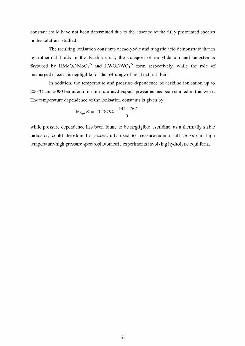
The resulting ionisation constants of molybdic and tungstic acid demonstrate that in
hydrothermal fluids in the Earth’s crust, the transport of molybdenum and tungsten is
favoured by HMoO4-/MoO4
2- and HWO4-/WO4
2- form respectively, while the role of
uncharged species is negligible for the pH range of most natural fluids.
In addition, the temperature and pressure dependence of acridine ionisation up to
200°C and 2000 bar at equilibrium saturated vapour pressures has been studied in this work.
The temperature dependence of the ionisation constants is given by,
TK 767.141178794.0log10 −−=
while pressure dependence has been found to be negligible. Acridine, as a thermally stable
indicator, could therefore be successfully used to measure/monitor pH in situ in high
temperature-high pressure spectrophotometric experiments involving hydrolytic equilibria.
iv
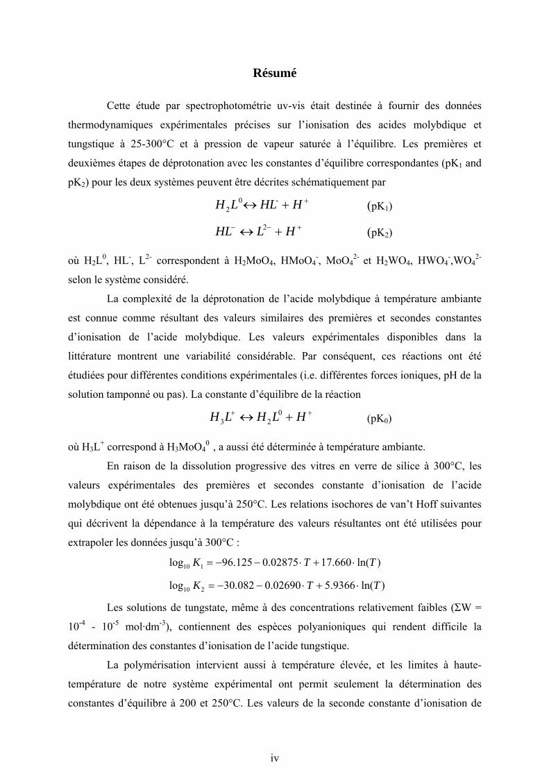
Résumé
Cette étude par spectrophotométrie uv-vis était destinée à fournir des données
thermodynamiques expérimentales précises sur l’ionisation des acides molybdique et
tungstique à 25-300°C et à pression de vapeur saturée à l’équilibre. Les premières et
deuxièmes étapes de déprotonation avec les constantes d’équilibre correspondantes (pK1 and
pK2) pour les deux systèmes peuvent être décrites schématiquement par ++↔ HHLLH -0
2 (pK1)
+−− +↔ HLHL 2 (pK2)
où H2L0, HL-, L2- correspondent à H2MoO4, HMoO4-, MoO4
2- et H2WO4, HWO4-,WO4
2-
selon le système considéré.
La complexité de la déprotonation de l’acide molybdique à température ambiante
est connue comme résultant des valeurs similaires des premières et secondes constantes
d’ionisation de l’acide molybdique. Les valeurs expérimentales disponibles dans la
littérature montrent une variabilité considérable. Par conséquent, ces réactions ont été
étudiées pour différentes conditions expérimentales (i.e. différentes forces ioniques, pH de la
solution tamponné ou pas). La constante d’équilibre de la réaction ++ +↔ HLHLH 0
23 (pK0)
où H3L+ correspond à H3MoO40 , a aussi été déterminée à température ambiante.
En raison de la dissolution progressive des vitres en verre de silice à 300°C, les
valeurs expérimentales des premières et secondes constante d’ionisation de l’acide
molybdique ont été obtenues jusqu’à 250°C. Les relations isochores de van’t Hoff suivantes
qui décrivent la dépendance à la température des valeurs résultantes ont été utilisées pour
extrapoler les données jusqu’à 300°C :
)ln(660.1702875.0125.96log 110 TTK ⋅+⋅−−=
)ln(9366.502690.0082.30log 210 TTK ⋅+⋅−−=
Les solutions de tungstate, même à des concentrations relativement faibles (ΣW =
10-4 - 10-5 mol·dm-3), contiennent des espèces polyanioniques qui rendent difficile la
détermination des constantes d’ionisation de l’acide tungstique.
La polymérisation intervient aussi à température élevée, et les limites à haute-
température de notre système expérimental ont permit seulement la détermination des
constantes d’équilibre à 200 et 250°C. Les valeurs de la seconde constante d’ionisation de

v
l’acide tungstique sont égales à 6.31 et 6.79 à 200 et 250°C respectivement. La première
constante d’ionisation n’a pas pu être déterminée en raison de l’absence d’espèces
complètement protonées dans les solutions étudiées.
Les constantes d’ionisation des acides molybdique et tungstique obtenues
démontrent que, dans les fluides hydrothermaux présents dans la croûte terrestre, le transport
de molybdène et de tungstène est favorisé par les formes HMoO4-/MoO4
2- et HWO4-/WO4
2-
respectivement, alors que le rôle des espèces non-chargées est négligeable sur la gamme de
pH de la plupart des fluides naturels.
De plus, la dépendance à la température et à la pression de l’ionisation de l’acridine
jusqu’à 200°C et 2000 bars à pression de vapeur saturée à l’équilibre a été étudiée dans ce
travail. La dépendance à la température de la constante d’ionisation est donnée par,
TK 767.141178794.0log10 −−=
et la dépendance à la pression a été trouvée négligeable. L’acridine, en tant qu’indicateur
thermiquement stable, pourrait ainsi être employée avec succès pour mesurer ou contrôler le
pH in situ dans des expériences spectrophotométriques haute-température haute-pression
impliquant des équilibres hydrolytiques.

1
1. Introduction
Molybdenum (Mo, atomic weight 95.94 and atomic number 42) and tungsten (W,
atomic weight 183.85 and atomic number 74) are both transition metals in group VI of the
Mendeleev’s Periodic Table. The complexity of their chemistry is due to the chemical
versatility of their possible oxidation states (from -2 to +6), various coordination numbers (4
to 8) and ability to form polynuclear complexes. They both occur naturally as a mixture of
several stable isotopes. Despite this similarity of chemical properties (including similar
atomic and ionic radii as well as electron affinity (KLETZIN and ADAMS, 1996 and references
therein) their geochemical and biochemical behavior is quite different.
Large quantities of tungsten are used in the production of hard materials containing
tungsten carbide as well as for ferrotungsten in the steel industry. Other uses are as catalysts
in the petroleum industry, as lubricating agents, in fluorescent lighting, and as pigments. The
microalloy of W with Al, K, and Si has been used since 1920 in light bulbs. Molybdenum is
used in various corrosion- and temperature-resistant alloys as well as a support for
semiconductors, in resistance filaments, in electrodes for the glass industry, as solid
lubricants and as an additive to special lubricating oils. Catalysts incorporating molybdenum
have many chemical engineering applications and various molybdates are employed as
thermally stable coloring agents and pigments. One of the most important reasons for the
increase in the use of molybdenum is its low toxicity (or intoxicity to human beings) so it
can be substituted for chromium or other toxic metals used in steel alloys (GUNTHER, 1980;
SEILER and SIGEL, 1988; LASSNER and SCHUBERT, 1999).
Mo and W compounds influence various life forms to varying degrees from toxic to
beneficial, but overall, they are only moderately toxic compared to other heavy metals,
though their toxicity is a function of chemical structure, solubility and route of
administration (SEILER and SIGEL, 1988).
Molybdenum, as well as tungsten, does not occur in metallic (elemental) form in
nature. It mostly occurs as sulphides with the oxidation state +4 (MoS2, molybdenite or its
amorphous modification jordisite), while the molybdate, powellite (CaMoO4), is a relatively
rare mineral. Tungsten is usually found as oxo-compounds in its highest oxidation state, +6,
as scheelite (CaWO4) or wolframite ((Fe,Mn)WO4), but its sulphide mineral, tungstenite
(WS2) is very rare. Minerals, such as wulfenite (PbMoO4), and stolzite (PbWO4), as well as
molybdite (MoO3), ilsemanite (Mo3O8·nH2O), tungstite (WO3·H2O) and elsmoreite

2
(WO3·0.5H2O) are known mostly as secondary minerals in oxidation zones of Mo and W
deposits (ARUTYUNYAN, 1966; URUSOV et al., 1967; IVANOVA et al., 1975; KOLONIN et al.,
1975; FOSTER, 1977).
The tungsten content of most rocks is similar to that of molybdenum, with the
average abundances in the Earth crust being about 1 to 1.55 ppb, but in surface waters W/Mo
ratio is lower (<0.5 ppb and <0.1 ppb Mo and W respectively) due to extensive adsorption
and / or precipitation onto ferric hydroxide / ferrihydrite, manganese oxide and clay minerals
(GUNTHER, 1980; KLETZIN and ADAMS, 1996; KISHIDA et al., 2004; ARNORSSON and
OSKARSSON, 2007). Both molybdenum and tungsten may be preferentially concentrated in
organic–rich sediments (KURODA and SANDELL, 1954; EMERSON and HUESTED, 1991)
though Arnorsson (2007) has noted that, unlike tungsten, only a small proportion of
molybdenum is removed from soil waters in peat environments. In surface waters,
molybdenum and tungsten occur dominantly as hexavalent oxy-anions, molybdate and
tungstate. In reducing H2S bearing solutions, the molybdenum, and to lesser extent tungsten,
may be removed to form molybdenite or tungstate or may coprecipitate with other sulphides.
In addition, the oxygen of the molybdate ions may be successively replaced by sulphur to
form thiomolybdates (EMERSON and HUESTED, 1991; BARLING et al., 2001; ROBB, 2005;
ARNORSSON and OSKARSSON, 2007).
It is known that both molybdenum and tungsten may occur in high concentrations in
superheated fumaroles of active volcanoes and hydrothermal discharges (PLIMER, 1980;
FULP and RENSHAW, 1985; HEDENQUIST and HENLEY, 1985; SEWARD and SHEPPARD, 1986;
WILLIAMS-JONES and HEINRICH, 2005; REMPEL et al., 2006; ARNORSSON and OSKARSSON,
2007). Hydrothermal vents in the deep sea (e.g. white and black smokers) also show
enrichment in these elements (CARPENTER and GARRETT, 1959; KLETZIN and ADAMS, 1996;
KISHIDA et al., 2004).
The temperature range for the formation of the molybdenum and tungsten deposits is
quite wide. For example, it has been shown that the temperature of the formation of
porphyry molybdenum deposits is generally around 550°C (e.g. ROSS et al., 2002) whereas
the temperatures of Mo-rich skarns vary from 500 to 600°C at approximately 400Mpa (e.g.
LENTZ and SUZUKI, 2000). Volcanic gas sublimation temperatures for molybdenite and
wolframite may be at t>500°C (e.g. WILLIAMS-JONES and HEINRICH, 2005). Ivanova (1986)
demonstrated, that scheelite can crystallize in nature over an extremely wide range of
physico-chemical conditions (temperature range: 150 to 600°C, 2-75 wt.% equivalent NaCl,
pressure 200-1600 bars). Shelton et al. (1987) has shown, that in the Dae Hwa W-Mo

3
deposit (Republic of Korea) the deposition of molybdenite, cassiterite, wolframite and early
scheelite occurred with decreasing temperature from 400°C to 230°C in response to
inundation of an original magmatic fluid system with low-temperature waters of meteoric
origin.
Hydrothermal tungsten transport and deposition by fluids in the Earth’s crust also
takes place in a lower temperature regime. For example, microthermometric measurements
and fluid inclusions in quartz and scheelite of Ixtahuacan Sb-W deposits (GUILLEMETTE and
WILLIAMS-JONES, 1993) point to a low temperature(160-190°C) and low salinity (5-15 wt%
NaCl eq.) of aqueous fluid. The usual temperatures of convective systems, including
hydrothermal vents in the seafloor are about 320-363 °C (BARNES, 1997; KISHIDA et al.,
2004), while geothermal waters vary between 40 and 325°C (e.g. (ARNORSSON and
IVARSSON, 1985; HEDENQUIST and HENLEY, 1985; SEWARD and SHEPPARD, 1986) may also
transport and deposit tungsten.
In magmatic hydrothermal fluids as well as geothermal waters, mononuclear
hydroxycomplexes dominate the speciation of molybdenum and tungsten, which are in
hexavalent state (KOLONIN et al., 1975; CANDELA and HOLLAND, 1984; ARNORSSON and
IVARSSON, 1985; STEMPROK, 1990; KEPPLER and WYLLIE, 1991). A recent EXAFS study of
Hoffmann (2000) has shown, that tungsten monomer, WO42-, remains tetrahedrally
coordinated at elevated temperatures (up to 400°C) with an unchanged W-O bond distance.
In addition to molybdic and tungstic acids (H2MoO40 and H2WO4
0) and their dissociation
products (MoO42-, HMoO4
−, WO42-, HWO4
− ), it has also been suggested that other species
such as KWO4− , NaWO4
− (WOOD and SAMSON, 2000), and NaHMoO40 and KHMoO4
0
(KUDRIN, 1989) may be responsible for the transport of molybdenum and tungsten in
hydrothermal fluids at high temperatures (≥300°C). In reducing conditions transport of
molybdenum can be carried out in lower (+4) valency state (KUDRIN, 1985; ROBB, 2005).
The experimental studies have shown, that the partitioning of molybdenum in
magmatic systems is independent of the chlorine content of magmas and associated aqueous
phases (CANDELA and HOLLAND, 1984). Fluoride does not appear to be essential for the
concentration of Mo and W in fluids evolving from granitic magma (CANDELA and
HOLLAND, 1984; KEPPLER and WYLLIE, 1991; LENTZ and SUZUKI, 2000), although
Tugarinov (1973) considered the transport of molybdenum in form of fluoride complexes in
acid solutions at high temperatures to be important.
Arutyunyan (1966) has suggested that thiomolybdate complexes may play an
important role in the transport of molybdenum in high temperatures systems. Later it was

4
shown, that thiomolybdate complexes cannot be responsible for transport of molybdenum
due to insufficient concentrations of sulphur in hydrothermal solutions (according to his
estimations, the necessary concentration of H2S is about 1 mol/kg (TUGARINOV et al., 1973),
while Kolonin showed spectrophotmetrically decomposition of those complexes at the
temperatures ≥100°C (KOLONIN and LAPTEV, 1975). More experimental studies are required.
Molybdenum stable isotope geochemistry may act as a potential proxy in paleoredox
applications due to its sensitivity to redox conditions, the clear difference in δ97/95Mo in the
anoxic and oxic sediments and various coordination geometries in mononuclear species
(which could drive isotope fractionation) (BARLING et al., 2001; SIEBERT et al., 2003;
ANBAR, 2004; ARNORSSON and OSKARSSON, 2007).
Unlike tungsten, molybdenum is an essential element for animals and plants.
Molybdenum-containing enzymes (e.g. xanthine oxydase, nitrate reductase) are ubiquitous in
nature and have been found in the vast majority of different forms of life (GUNTHER, 1980;
SEILER and SIGEL, 1988) . It is notable that there appears to be a marked interaction between
W and Mo when both are present in their oxy-anion forms: it is easier to induce Mo
deficiency by feeding animals tungstate than by attempting to eliminate Mo from the diet,
and the symptoms of tungsten toxicity can be counteracted by supplementing the diet with
molybdate, suggesting that tungstate competes with molybdate at biochemically active sites
in animals (GUNTHER, 1980 and references therein). Only recently, four distinct types of
tungstoenzyme have been purified from various microbial sources. Most of the
tungstoenzymes have analogous Mo-containing counterparts in the same or closely related
organism. It is interesting, however, that the enzymes in hyperthermophilic bacteria appear
to be obligately tungsten dependent (KLETZIN and ADAMS, 1996; LASSNER and SCHUBERT,
1999). This perhaps lends support to numerous speculations that it may not be coincidental
that life has been proposed to have originated at extreme temperatures in deep sea
hydrothermal systems and that at least some of the present-day marine hyperthermophiles
appear to be obligately W-dependent. In addition to availability, a key factor in tungsten
utilization appears to be its redox properties relative to molybdenum. Tungsten –containing
enzymes might therefore be considered as a precursors to molybdenum-containing enzymes
and as an ancient redox cofactor (KLETZIN and ADAMS, 1996).
The hydrothermal geochemistry and biogeochemistry of molybdenum and tungsten
demand precise thermodynamic data which are currently almost unavailable. The aim of this
study has therefore been to obtain fundamental thermodynamic data for the deprotonation /
ionisation of molybdic and tungstic acids (i.e. H2MoO4 and H2WO4) at temperatures from 25

5
to 300 °C and at pressures near the equilibrium saturated vapour pressure. The temperature
and pressure dependence of acridine ionisation was also studied. Being a thermally stable
indicator, it can be used in spectroscopic measurements, allowing exact pH determination in
situ.
1.1. References Anbar A. D. (2004) Molybdenum stable isotopes: observations, interpretations and
directions. Reviews in Mineralogy & Geochemistry 55, 428-454. Arnorsson S. and Ivarsson G. (1985) Molybdenum in Icelandic geothermal waters.
Contributions to Mineralogy and Petrology 90(2-3), 179-89. Arnorsson S. and Oskarsson N. (2007) Molybdenum and tungsten in volcanic rocks and in
surface and <100 DegC ground waters in Iceland. Geochimica et Cosmochimica Acta 71(2), 284-304.
Arutyunyan L. A. (1966) The stability of water-soluble forms of molybdenum in sulphur-containing solutions at high temperatures. Geokhimiya 4, 479-482.
Barling J., Arnold G. L., and Anbar A. D. (2001) Natural mass-dependent variations in the isotopic composition of molybdenum. Earth and Planetary Science Letters 193(3-4), 447-457.
Barnes H. L. (1997) Geochemistry of Hydrothermal Ore Deposits. 3d Ed. Candela P. A. and Holland H. D. (1984) The partitioning of copper and molybdenum
between silicate melts and aqueous fluids. Geochimica et Cosmochimica Acta 48(2), 373-80.
Carpenter L. G. and Garrett D. E. (1959) Tungsten in Searles Lake. Mining Engineering (Littleton, CO, United States)(11), 301-3.
Emerson S. R. and Huested S. S. (1991) Ocean anoxia and the concentrations of molybdenum and vanadium in seawater. Marine Chemistry 34(3-4), 177-96.
Foster R. P. (1977) Solubility of scheelite in hydrothermal chloride solutions. Chemical Geology 20(1), 27-43.
Fulp M. S. and Renshaw J. L. (1985) Volcanogenic-exhalative tungsten mineralization of Proterozoic age near Santa Fe, New Mexico, and implications for exploration. Geology 13(1), 66-9.
Guillemette N. and Williams-Jones A. E. (1993) Genesis of the antimony-tungsten-gold deposits at Ixtahuacan, Guatemala: evidence from fluid inclusions and stable isotopes. Mineralium Deposita 28(3), 167-80.
Gunther F. A. (1980) Residue Reviews, Vol. 74: Residues of Pesticides and Other Contaminants in the Total Environment.
Hedenquist J. W. and Henley R. W. (1985) Hydrothermal eruptions in the Waiotapu geothermal system, New Zealand: their origin, associated breccias, and relation to precious metal mineralization. Economic Geology and the Bulletin of the Society of Economic Geologists 80(6), 1640-68.
Hoffmann M. M., Darab J. G., Heald S. M., Yonker C. R., and Fulton J. L. (2000) New experimental developments for in situ XAFS studies of chemical reactions under hydrothermal conditions. Chemical Geology 167(1-2), 89-103.
Ivanova G. F., Levkina N. I., Nesterova L. A., Zhidikova A. P., and Khodakovskii I. L. (1975) Equilibria in the molybdenum trioxide-water system in the 25-300°C range. Geokhimiya 2, 234-247.

6
Ivanova G. F., Naumov V. B., and Kopneva L. A. (1986) Physico-chemical parameters of formation of scheelite in ore deposits of various genetic types based on a study of fluid inclusions. Geokhimiya(10), 1431-42.
Keppler H. and Wyllie P. J. (1991) Partitioning of copper, tin, molybdenum, tungsten, uranium and thorium between melt and aqueous fluid in the systems haplogranite-water-hydrogen chloride and haplogranite-water-hydrogen fluoride. Contributions to Mineralogy and Petrology 109(2), 139-50.
Kishida K., Sohrin Y., Okamura K., and Ishibashi J.-i. (2004) Tungsten enriched in submarine hydrothermal fluids. Earth and Planetary Science Letters 222(3-4), 819-827.
Kletzin A. and Adams M. W. W. (1996) Tungsten in biological systems. FEMS Microbiology Reviews 18(1), 5-63.
Kolonin G. R. and Laptev Y. V. (1975) Spectrophotometric study of temperature influence on tiomolybdate complexes. in Experimental Studies in Mineralogy, Akad. Nauk USSR, Novosibirsk, 38-43.
Kolonin G. R., Laptev Y. V., and Biteikina R. P. (1975) Formation Condition of Molybdenite and Powellite in Hydrotermal Solutions. in Experimental Studies in Mineralogy, Akad. Nauk USSR, Novosibirsk, 27-33.
Kudrin A. V. (1985) Experimental study of solubility of tugarinovite MoO2 in aqueous solutions at high temperatures. . Geokhimiya 6, 870-83.
Kudrin A. V. (1989) Behavior of Mo in aqueous NaCl and KCl solutions at 300-450°C. Geokhimiya 1, 99-112.
Kuroda P. K. and Sandell E. B. (1954) Geochemistry of molybdenum. Geochimica et Cosmochimica Acta 6, 35-63.
Lassner E. and Schubert W.-D. (1999) Tungsten: Properties, Chemistry, Technology of the element , Alloys, and Chemical Compounds. Plenum Publishers.
Lentz D. R. and Suzuki K. (2000) A low F pegmatite-related mo skarn from the southwestern Grenville province, Ontario, Canada: phase equilibria and petrogenetic implications. Economic Geology and the Bulletin of the Society of Economic Geologists 95(6), 1319-1337.
Plimer I. R. (1980) Exhalative tin and tungsten deposits associated with mafic volcanism as precursors to tin and tungsten deposits associated with granites. Mineralium Deposita 15(3), 275-89.
Rempel K. U., Migdisov A. A., and Williams-Jones A. E. (2006) The solubility and speciation of molybdenum in water vapour at elevated temperatures and pressures: Implications for ore genesis. Geochimica et Cosmochimica Acta 70(3), 687-696.
Robb L. J. (2005) Introduction to ore-forming processes. Blackwell Publishing Company. Ross P.-S., Jebrak M., and Walker B. M. (2002) Discharge of hydrothermal fluids from a
magma chamber and concomitant formation of a stratified breccia zone at the Questa porphyry molybdenum deposit, New Mexico. Economic Geology 97(8), 1679-1699.
Seiler H. G. and Sigel H. (1988) Handbook on toxicity of inorganic compounds. Seward T. M. and Sheppard D. S. (1986) Waimangu geothermal field. in: Monograph Series
on Mineral Deposits 26, 81-91. Shelton K. L., Taylor R. P., and So C. S. (1987) Stable isotope studies of the Dae Hwa
tungsten-molybdenum mine, Republic of Korea: Evidence of progressive meteoric water interaction in a tungsten-bearing hydrothermal system. Economic Geology and the Bulletin of the Society of Economic Geologists 82(2), 471-81.
Siebert C., Nagler T. F., von Blanckenburg F., and Kramers J. D. (2003) Molybdenum isotope records as a potential new proxy for paleoceanography. Earth and Planetary Science Letters 211(1-2), 159-171.

7
Stemprok M. (1990) Solubility of tin, tungsten, and molybdenum oxides in felsic magmas. Mineralium Deposita 25(3), 205-12.
Tugarinov A. I., Khodakovskii I. L., and Zhidikova A. P. (1973) Physicochemical conditions of molybdenite formation in hydrothermal uranium-molybdenum deposits. Geokhimiya 7, 975-984.
Urusov V. S., Ivanova G. F., and Khodakovskii I. L. (1967) Energy and thermodynamic characteristics of tungstates and molybdates in connection with some features of their geochemistry. Geokhimiya(10), 1050-63.
Williams-Jones A. E. and Heinrich C. A. (2005) 100th anniversary special paper. Vapor transport of metals and the formation of magmatic-hydrothermal ore deposits. Economic Geology 100(7), 1287-1312.
Wood S. A. and Samson I. M. (2000) The hydrothermal geochemistry of tungsten in granitoid environments: I. Relative solubilities of ferberite and scheelite as a function of T, P, pH, and mNaCl. Economic Geology and the Bulletin of the Society of Economic Geologists 95(1), 143-182.
8
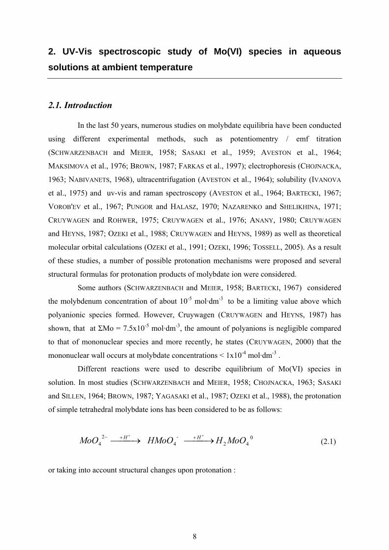
2. UV-Vis spectroscopic study of Mo(VI) species in aqueous solutions at ambient temperature
2.1. Introduction
In the last 50 years, numerous studies on molybdate equilibria have been conducted
using different experimental methods, such as potentiomentry / emf titration
(SCHWARZENBACH and MEIER, 1958; SASAKI et al., 1959; AVESTON et al., 1964;
MAKSIMOVA et al., 1976; BROWN, 1987; FARKAS et al., 1997); electrophoresis (CHOJNACKA,
1963; NABIVANETS, 1968), ultracentrifugation (AVESTON et al., 1964); solubility (IVANOVA
et al., 1975) and uv-vis and raman spectroscopy (AVESTON et al., 1964; BARTECKI, 1967;
VOROB'EV et al., 1967; PUNGOR and HALASZ, 1970; NAZARENKO and SHELIKHINA, 1971;
CRUYWAGEN and ROHWER, 1975; CRUYWAGEN et al., 1976; ANANY, 1980; CRUYWAGEN
and HEYNS, 1987; OZEKI et al., 1988; CRUYWAGEN and HEYNS, 1989) as well as theoretical
molecular orbital calculations (OZEKI et al., 1991; OZEKI, 1996; TOSSELL, 2005). As a result
of these studies, a number of possible protonation mechanisms were proposed and several
structural formulas for protonation products of molybdate ion were considered.
Some authors (SCHWARZENBACH and MEIER, 1958; BARTECKI, 1967) considered
the molybdenum concentration of about 10-5 mol·dm-3 to be a limiting value above which
polyanionic species formed. However, Cruywagen (CRUYWAGEN and HEYNS, 1987) has
shown, that at ΣMo = 7.5x10⁻⁵ mol·dm-3, the amount of polyanions is negligible compared
to that of mononuclear species and more recently, he states (CRUYWAGEN, 2000) that the
mononuclear wall occurs at molybdate concentrations < 1x10⁻⁴ mol·dm-3 .
Different reactions were used to describe equilibrium of Mo(VI) species in
solution. In most studies (SCHWARZENBACH and MEIER, 1958; CHOJNACKA, 1963; SASAKI
and SILLEN, 1964; BROWN, 1987; YAGASAKI et al., 1987; OZEKI et al., 1988), the protonation
of simple tetrahedral molybdate ions has been considered to be as follows:
042
-4
24 MoOHHMoOMoO HH ⎯⎯ →⎯⎯⎯ →⎯
++ ++− (2.1)
or taking into account structural changes upon protonation :

9
02222
-3
24 )()( )( OHOHMoOOHMoOMoO HH ⎯⎯ →⎯⎯⎯ →⎯
++ ++− (2.2)
Cjojnacka (1963) and Cruywagen (1976) have proposed the further protonation of
neutral molybdic acid to form H3MoO4+ and H4MoO4
2+. A number of studies have been
carried out on the hydrolysis of molybdenil ion (MoO2 2+) (VOROB'EV et al., 1967;
NABIVANETS, 1968; NAZARENKO and SHELIKHINA, 1971; IVANOVA et al., 1975) . These
reactions can be summarized by the following scheme,
−
+++++
=
⎯⎯ →⎯=⎯⎯ →⎯⎯⎯ →⎯-
432
042222
22
)(
)( 222
HMoOOHMoO
MoOHOHMoOOHMoOMoO OHOHOHKh1 Kh2 Kh3
(2.3)
In this case, the third hydrolysis constant, Kh3, is equivalent to the first ionisation constant of
molybdic acid.
The discussion in the literature has centred around the coordination of molybdenum
in different molybdate species and therefore their correct formulas. For many oxyacids, the
protonation / deprotonation constants differ by at least four orders of magnitude. The
unusually close values for first and second ionisation constants of molybdic acid (see table
2.1) were explained by an increase of coordination number from 4 (tetrahedral -24MoO ) to
6 by protonation. Initially it was thought that an increase in coordination number occurs
during the first protonation step (SCHWARZENBACH and MEIER, 1958) and therefore, the
formula of -4HMoO should be more correctly written as )( -5OHMoO . The first
protonation constant was considered abnormally low due to a decrease in entropy
accompanying the immobilisation of two water molecules. Later on it was suggested by
Cruywagen and Rohwer (1975) that there is a considerable negative volume change for the
second protonation, which is due to an increase in coordination number and therefore the
second protonation constant should be regarded as abnormally large and the first as normal.
The formulation, )( -5OHMoO , was also concluded to be doubtful (CRUYWAGEN and
HEYNS, 1989). Several “correct” formulas for molybdic acid were proposed such as
)( 6OHMo (CRUYWAGEN and ROHWER, 1975) , )()( 2222 OHOHMoO (TYTKO, 1986) and
)( 323 OHMoO (PAFFETT and ANSON, 1981) . The formula )( 6OHMo may be used for
convenience to indicate 6 coordination, but electrostatic calculations (CRUYWAGEN and

10
HEYNS, 1989) predict an increase in stability from )( 6OHMo to )()( 2222 OHOHMoO and
)( 323 OHMoO with a regular octahedral with no changes in bond length. Molecular orbital
calculations (OZEKI, 1996) indicate that molybdic acid has a kind of distorted octahedral
structure, consisting of three Mo-O bond lengths of 1.68Å, 1.99Å and 2.38Å, which is
consistent with an )()( 2222 OHOHMoO structure, but )( 323 OHMoO was not taken into
account in calculations. More recent molecular orbital calculations (TOSSELL, 2005)
eliminated the existence of )( 06OHMo , giving preference to its isomers
02222 )()( OHOHMoO and )( 0
323 OHMoO which have similar energy. In this work, the
alternative species, 03MoO , with more favourable energy has also been proposed. For
simplicity, we have chosen to use the formulation, 42 MoOH , for molybdic acid monomer
throughout this work.
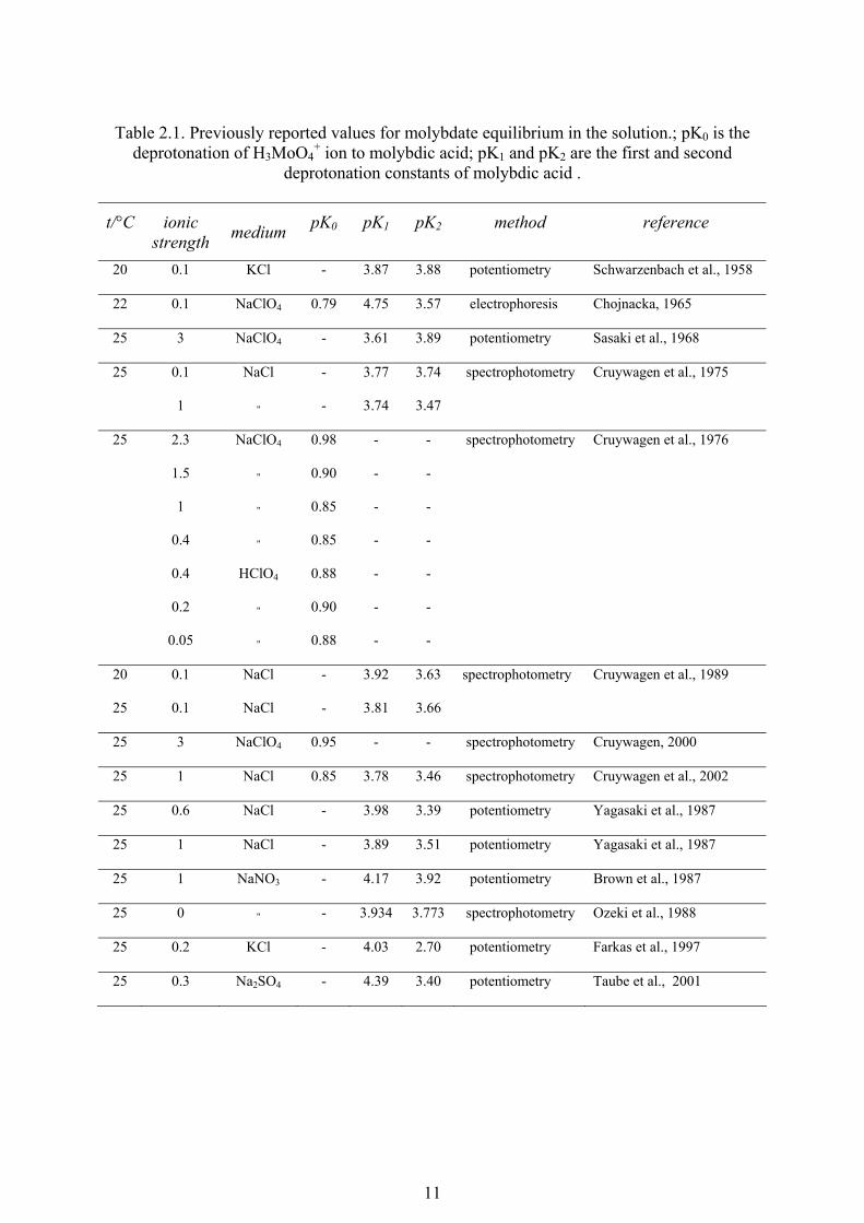
Table 2.1 gives the literature experimental values of ionisation constants for
molybdic acid. The considerable scatter may be explained to a large extent by differences in
experimental methods and conditions. The similarity in values of pK1 and pK2 may also
create difficulties in the mathematical treatment of experimental data. In this work, we have
determined ionisation constants of molybdic acid using three different series of experiments.
In the first series (Appendix 2.7.1), the pH (2.5<pH<5.4) was adjusted with perchloric acid,
and the ionic strength was not adjusted (varied between 5x10⁻³ and 8x10⁻⁴ mol·dm-3). In the
second series of solutions (Appendix 2.7.2), the ionic strength was kept constant by additions
of HClO4 / NaClO4. In this series, solutions with five different ionic strengths (0.10, 0.30,
0.62, 1.08, 3.46 mol·dm-3 ) were studied within the pH range 2.3<pH<5.2. In the third series
(Appendix 2.7.3), the pH varied within the range 0.46<pH<5.5 with perchloric acid and in
some cases (higher pH) buffered by an acetic acid / acetate buffer. The ionic strength was
adjusted with NaClO4 to four ionic strengths (0.10, 0.28, 0.56, 0.90 mol·dm-3). In addition,
one set of solutions (set I, Appendix 2.7.3) for which the ionic strength was not adjusted (i.e.
not kept constant) was also considered.
11
Table 2.1. Previously reported values for molybdate equilibrium in the solution.; pK0 is the
deprotonation of H3MoO4+ ion to molybdic acid; pK1 and pK2 are the first and second
deprotonation constants of molybdic acid .
t/°C ionic strength medium pK0 pK1 pK2 method reference
20 0.1 KCl - 3.87 3.88 potentiometry Schwarzenbach et al., 1958
22 0.1 NaClO4 0.79 4.75 3.57 electrophoresis Chojnacka, 1965
25 3 NaClO4 - 3.61 3.89 potentiometry Sasaki et al., 1968
25 0.1 NaCl - 3.77 3.74 spectrophotometry Cruywagen et al., 1975
1 " - 3.74 3.47
25 2.3 NaClO4 0.98 - - spectrophotometry Cruywagen et al., 1976
1.5 " 0.90 - -
1 " 0.85 - -
0.4 " 0.85 - -
0.4 HClO4 0.88 - -
0.2 " 0.90 - -
0.05 " 0.88 - -
20 0.1 NaCl - 3.92 3.63 spectrophotometry Cruywagen et al., 1989
25 0.1 NaCl - 3.81 3.66
25 3 NaClO4 0.95 - - spectrophotometry Cruywagen, 2000
25 1 NaCl 0.85 3.78 3.46 spectrophotometry Cruywagen et al., 2002
25 0.6 NaCl - 3.98 3.39 potentiometry Yagasaki et al., 1987
25 1 NaCl - 3.89 3.51 potentiometry Yagasaki et al., 1987
25 1 NaNO3 - 4.17 3.92 potentiometry Brown et al., 1987
25 0 " - 3.934 3.773 spectrophotometry Ozeki et al., 1988
25 0.2 KCl - 4.03 2.70 potentiometry Farkas et al., 1997
25 0.3 Na2SO4 - 4.39 3.40 potentiometry Taube et al., 2001

12
2.2. Experimental
All the solutions were prepared on a molal scale with Nanopure Millipore water
(resistivity >18MΩ/cm). Stock solutions of acids (hydrochloric, perchloric) were diluted
from concentrated acids (perchloric acid, 60%, p.a., Merck; hydrochloric acid, 30%,
suprapur, Merck) and standardized by colorimetric titration against Trizma-base
(Ttris(hydroxymethyl)aminomethane, 99+%,Aldrich) using methyl red as an indicator and
potentiometric titration, using a universal pH glass electrode (Metrohm). Stock solutions of
acetic acid and sodium acetate were prepared by weight from glacial acetic acid (100%,
extra pure, Merck) and sodium acetate salt (sodium acetate anhydrous, Fluka, ≥99.5%).
Sodium perchlorate solutions were prepared from sodium perchlorate monohydrate salt
(Aldrich) and used as absorbance blanks (optical cell windows + solution) as required.
Sodium molybdate stock solution (10-2 mol·kg-1) was prepared by dissolving of sodium
molybdate dihydrate salt (99.99%, Aldrich) in nanopure Millipore water and stored in a
polyethylene bottle. The presence of two molecules of water in Na2MoO4·2H2O was
confirmed by weighing before and after drying of a given amount of salt at 105°C until a
constant weight was attained. All others solutions of sodium molybdate were prepared by
dilution (by weight) of stock solution. The total molybdenum (i.e. molybdate) concentration
was always maintained at <10-4 mol·dm-3 in order to avoid the formation of polynuclear
species.
The stability of sodium molybdate solutions was monitored spectrophotometrically
to ensure that in solutions prepared by dilution of more concentrated stock solution, there
was no “memory effect” involving polymerisation. Five solutions of approximately 1x10⁻⁵
mol·dm-3 concentration were prepared from stock solutions prepared at different times and
then the UV spectra were measured on the same day under the same conditions. An absence
of any “memory effect” in the solutions as a function of time was confirmed by the spectra
shown in fig.2.1 which are identical despite differences in the way they were prepared and
stored. Note, that the normalised absorbance refers to the measured absorbance divided (i.e.
normalised) by the molybdenum concentration for the purpose of comparison.
The first two series of solutions were analyzed with a CARY 5 double beam
spectrophotometer at 24°C and the last series with Cary 50 at 22°C. Spectra were taken in a
silica glass cuvette (1cm path length) over the 190-500 nm wavelength range at 0.5nm
intervals with a scanning rate of 100 nm/min. For each solution, an average of 3 spectra was
measured. All spectra were corrected for background absorbance (windows + water +

13
200 210 220 230 240 250 260 2700
1000
2000
3000
4000
5000
6000
7000
8000
9000
10000
Wavelength / nm
Nor
mal
ized
Abs
orba
nce
s1s2s3s4s5
Fig.2.1 Spectra (normalised absorbance) of Mo(VI)- containing solutions prepared by dilution of stock solutions of varying age; solution 1 prepared from 10-3 mol·kg-1 fresh stock solution (prepared at the same day); solution 2 prepared from 10-2 mol·kg-1 fresh stock solution; solution 3 is a solution, prepared from 10-2 mol·kg-1 stock solution and then “aged” for three month; solution 4 prepared from 3 month old 10-2 mol·kg-1 stock solution; solution 5 prepared from 6 month old 10-2 mol·kg-1 stock solution.

14
190 200 210 220 230 240 250 260 270 2800
0.2
0.4
0.6
0.8
1
1.2
1.4
1.6
1.8A
bsor
banc
e
Wavelength / nm
0.02100.00480.00270.00130.00080.00060.0002
[CH3COONa], mol/dm3
200 220 240 260 280 300
0
0.1
0.2
0.3
0.4
0.5
0.6
Wavelength / nm
Abs
orba
nce
0.00960.00400.00190.00090.0004
[CH3COOH], mol/dm3
200 220 240 260 280 300
0
0.1
0.2
0.3
0.4
0.5
0.6
0.7
0.8
0.9
1
Wavelength / nm
Abs
orba
nce
0.0460.1020.3020.6020.974
[NaClO4], mol/dm3
200 220 240 260 280 3000
0.05
0.1
0.15
0.2
Wavelength / nm
Abs
orba
nce
0.010
0.040
0.074
0.187
[HClO4], mol/dm3
200 210 220 230 240 250 2600
20
40
60
80
100
120
140
160
Wavelength / nm
Mol
ar a
bsor
ptiv
ity
CH3COOHCH3COO-ClO4-Na+
Fig.2.2. Spectra and molar absorptivity for the components of background absorbance at 22°C.

15
dissolved salts, absorbances of which were measured separately in the same cuvette at the
same temperature, see fig.2.2)
2.3. Data Treatment
Assuming that the speciation in solutions having Mo concentrations below the
“mononuclear wall” (i.e. ΣMo <10-4 mol·dm-3 ) is quite well established and for the case
when there are 3 absorbing species (H2MoO4, HMoO4 , MoO4
2) in studied pH interval (i.e.
2.5<pH<5.5), the following chemical model can be ascribed which involves,
(i) deprotonation equilibrium of molybdic acid,
[ ] [ ][ ]LH
HHLK HHL
21
+− ⋅⋅⋅=
+− γγ (2.4)
[ ] [ ][ ] ⋅⋅
⋅⋅⋅=
−
+−
−
+−
HL
HL
HL
HLK
γ
γγ2
2
2
(2.5)
where H2L, HL-, L2- correspond to H2MoO4, HMoO4-, MoO4
2- respectively.
(ii) the ion product constant of water:
[ ] [ ] −+ ⋅⋅⋅= −+OHHw OHHK γγ (2.6)
(iii) charge balance equations:
[ ] [ ] [ ] [ ] [ ] [ ]++−−−− +=+++ NaHClOOHLHL 422
(2.7)
(iv) mass balance equations for total molybdenum:
[ ] [ ] [ ] [ ]−− ++= 22 LHLLHLtot
(2.8)
The terms in square brackets are molal concentrations and γ is the molal activity
coefficient of the corresponding species and is taken as unity for uncharged species. Molar
concentrations of absorbing species used in Beer’s law in the cases when ionic strength was
not adjusted were calculated using the density of water taken from Wagner (1998) (given the
low concentration of solution components). Molar concentrations of absorbing species at
different ionic strengths were calculated using the density of sodium perchlorate of
corresponding concentrations (JANZ et al., 1970). Values of wK were taken from Marshall

16
and Franck (1981). Activity coefficients for charged species were calculated using an
extended Debye-Hückel equation of the form:
IBaIAz
i
ii 0
2
10 1log
+−=γ (2.9)
where the Debye-Hückel limiting slope parameters A, B where taken from Fernandez
(1997). The iterative calculation procedure was based on successive substitution with the
initial assumption that all the activity coefficients were equal to unity.
For case 3 (0.46<pH<5.5, buffered with the acetate buffer), the deprotonation of
H3MoO4+ to molybdic acid was considered, i.e.
++ +↔ HMoOHMoOH 04243 (2.10)
for which,
[ ] [ ][ ] +
+
⋅
⋅⋅= +
+
LH
H
LHHLH
K3
3
02
0 γγ (2.11)
where H3L+corresponds to H3MoO4+,
The relevant equilibrium constants for sodium acetate and acetic acid are given by,
[ ] [ ][ ]COONaCH
NaCOOCHK NaCOOCH
acetate3
33
+− ⋅⋅⋅=
+− γγ (2.12)
[ ] [ ][ ]COOHCH
HCOOCHK HCOOCH
acetic3
33
+− ⋅⋅⋅=
+− γγ (2.13)
Respective changes to the charge balance and mass balance (for total Na, acetate and
molybdenum) equations were introduced:
[ ] [ ] [ ] [ ] [ ] [ ] [ ] [ ]+++−−−−− ++=+++∗+ LHNaHClOOHCOOCHLHL 34322
(2.14)
[ ] [ ]++= NaCOONaCHNatot 3 (2.15)
[ ] [ ] [ ] [ ]−++= COOCHCOONaCHCOOHCHCOOCH tot 3333 (2.16)

17
[ ] [ ] [ ] [ ] [ ]−−+ +++= 223 LHLLHLHLtot
(2.17)
For the cases where ionic strength was kept constant (i.e. cases 2 and 3), the activity
coefficients were not taken into consideration and therefore the apparent equilibrium
constants, K*, were obtained. As an approximation, the apparent constants for K*w, K*
acetate,
K*acetic were taken from Busey and Mesmer (BUSEY and MESMER, 1978), Mesmer et al.
(1989) and Shock et al. (1993) and refer to NaCl media having the same ionic strength as the
studied solutions.
The collected spectra were stored as an absorbance matrix Ai×j (where i- number of
wavelengths, j – number of analyzed solutions) and were corrected for background
absorbance (i.e. cell+solvent+perchlorate ion). For each matrix corresponding to different
total molybdenum concentrations, we applied a singular value decomposition (SVD) in order
to determine the number of absorbing species required for the chemical model (see details
elsewhere (MINUBAYEVA et al., 2008)
The molybdic acid ionisation (deprotonation) constants, K1 and K2, were optimized
simultaneously by solving equation,
ε×C = A = U i×n × S n×n × V j×n T , (2.18)
The left part of equation (2.18) represents Beer’s law, where ε is the i×n matrix of molar
absorptivities and C is the n×j matrix of molar concentrations of absorbing species obtained
from the solution of a system of ten linear equations describing the chosen chemical model
(see above) . The right side of the equation is the SVD (singular value decomposition) of
absorbance matrix A with n absorbing species. The calculation procedure is similar to that
described by Boily and Suleimenov (BOILY and SULEIMENOV, 2006). All calculations have
been carried out with Maple (analytical solution of a system of equations) and Matlab
platforms (matrix manipulation and optimization, see Appendices, 7D).
2.4. Results and discussion
2.4.1. Case 1. pH and ionic strength vary (I< 5.00x10⁻³ mol·dm-3).
The spectra of a series of molybdate containing solutions over a range of varying
pH are shown in fig.2.3. Note, that indicated total molybdenum concentrations refer to the
average Mo concentration for the pH range shown. We can see that as the deprotonation of
molybdic acid proceeds (fig. 2.4a, 5.5>pH>4.21), the maximum of the spectra (at 208 nm)

18
undergoes a red shift. The shoulder at 230 nm flattens out and a weak band at 265 nm
appears. An isosbestic point occurs at 243.5 nm. As a result of further ionisation in the
4.21>pH>3.55 pH interval (fig. 2.4b), a distinct change in the absorption spectra takes place.
In the 3.55>pH>2.51 (fig. 2.4c) interval, an increase in the absorbance (for the main part as
well as for the tail) can be observed with the small red shift of the maximum from 218 to 219
nm. Two isosbectic points occur at 212 and 252.5 nm. For pH≤ 2.51 (fig. 2.4d), the tail at
265 nm continues to grow while the maximum in the spectra rapidly decreases and shifts
towards the far UV region. Two isosbestic points occur at 207 and 254 nm and the maximum
shifts form 211 to 218 nm.
200 220 240 260 280 300 320 3400
1000
2000
3000
4000
5000
6000
7000
8000
9000
10000
Wavelength / nm
Nor
mal
ized
Abs
orba
nce
0.360.670.981.191.491.782.062.272.512.853.193.553.704.064.214.464.714.955.205.50
pH=5.50
pH=0.36
pH
pH=2.51
5.50 0.36
Fig.2.3. Spectra (normalised absorbance) of Mo(VI)-containing solutions with
0.36<pH<5.5 and total Mo concentration 5.6x10⁻⁵ mol·dm-3 at 22°C.
The ultraviolet spectra were measured for 10 sets of solutions (see Appendix 2.7.1)
in which the total molybdenm varied from 9.39x10⁻⁶ mol·dm-3 to 1.09x10⁻⁴ mol·dm-3 and pH
was within interval, 2.5<pH<5.5.
In fig.2.5, one can see the product of U and S matrixes plotted versus wavelength,
indicating the contribution of the most significant vectors to the absorption profile. For all
the experiments with ΣMo≤·5.6x10⁻⁵ mol·dm-3, three curves were distinguished, two of
which make a significant contribution to total absorbance, and the third, a very small
contribution. For the case, where ΣMo=1.1x10⁻⁴ mol·dm-3 one observes the contribution of a

19
a)20
022
024
026
028
030
032
034
0
0
2000
4000
6000
8000
1000
0
Normalisedabsorbance
Wav
elen
gth
/n
m
4.21
4.46
4.71
4.95
5.20
5.50
pH
pH
=5
.50
4.2
1
4.2
1
pH
=5
.50
b)200
250
300
350
0
1000
2000
3000
4000
5000
6000
7000
Wav
ele
ng
th /
nm
Normalisedabsorbance
3.55
3.70
4.06
4.21
pH
=4
.21
3.5
5
3.5
5
pH
=4
.21
pH
c)2
00
220
24
026
028
03
00
32
03
40
0
10
00
20
00
30
00
40
00
50
00
60
00
70
00
Wav
elen
gth
/n
m
Normalisedabsorbance
2.5
12
.85
3.1
93
.55
2.5
1
2.5
1
3.5
5
pH
=3.5
5
pH
d)20
022
024
026
028
030
032
034
00
1000
2000
3000
4000
5000
6000
7000
Wav
elen
gth
/n
mNormalisedabsorbance
0.67
0.98
1.19
1.49
1.78
2.06
2.27
2.51
pH=2.
51
0.6
7
0.6
7
pH=2
.51
pH
Fig.
2.4
Spe
ctra
(nor
mal
ised
abs
orba
nce)
of M
o(V
I)-c
onta
inin
g so
lutio
ns w
ith to
talM
o co
ncen
tratio
n 5.
6x10
-5m
ol·d
m-3
at 2
2°C
ana
lyze
d by
pH
inte
rval
s: (a
) 5.5
> p
H >
4.2
1; (b
) 4.2
1 >
pH>
3.55
; (c
) 3.5
5 >
pH >
2.5
1; (
d) 2
.51
> pH
> 0
.67.

20
a)
210 220 230 240 250 260
0.01
0.02
0.03
0.04
0.05
0.06
0.07
0.08
0.09
0.1
0.11
Wavelength / nm
Abs
orba
nce
5.204.894.624.514.414.304.194.134.003.903.673.493.313.142.962.52
pHpH=5.20
2.52
[Motot]=1.0e-05
210 220 230 240 250 260
-0.04
-0.02
0
0.02
0.04
0.06
0.08
0.1
0.12
Wavelength / nm
UxS
1
2
3
[Motot]=1.0e-05
b)
200 210 220 230 240 250 2600
0.05
0.1
0.15
0.2
0.25
Wavelength / nm
Abs
orba
nce
5.405.104.854.714.494.434.324.264.103.963.793.583.393.213.042.48
[Motot]=2.1e-05pHpH=5.40
2.48
210 220 230 240 250 260
-0.05
0
0.05
0.1
0.15
0.2
Wavelength / nm
UxS
1
2
3
[Motot]=2.1e-05
c)
210 220 230 240 250 260
0.05
0.1
0.15
0.2
0.25
0.3
0.35
0.4
Wavelength / nm
Abs
orba
nce
5.345.044.794.654.544.464.324.254.133.993.773.563.363.172.992.52
2.52
pH=5.34[Motot]=4.0e-05 pH
200 210 220 230 240 250 260
-0.2
-0.1
0
0.1
0.2
0.3
Wavelength / nm
UxS
1
3
2
[Motot]=4.0e-05

21
d)
200 210 220 230 240 250 2600
0.1
0.2
0.3
0.4
0.5
0.6
0.7
Wavelength / nm
Abs
orba
nce
5.104.964.744.644.504.464.304.163.923.683.463.263.062.53
[Motot]=5.6e-05
2.53
pH=5.10
pH
200 210 220 230 240 250 260-0.2
-0.1
0
0.1
0.2
0.3
0.4
Wavelength / nm
UxS
[Motot]=5.6e-05
1
3
2
e)
205 210 215 220 225 230 235 240 245 250 255
0.2
0.4
0.6
0.8
1
1.2
Wavelength / nm
Abs
orba
nce
5.485.174.934.804.714.624.494.454.324.193.993.743.493.263.062.54
pH[Motot]=1.1e-04
pH=5.48
2.54
210 220 230 240 250 260
-0.2
0
0.2
0.4
0.6
0.8
Wavelength / nm
UxS
1
3
2
4?
[Motot]=1.1e-04
Fig.2.5. Spectra of experimental solutions with different total Mo(VI) concentrations at I=0 and contribution of most significant factors in total absorbance. Total molybdenum
concentrations (indicated in this figure and further on) refer to the average Mo concentration for the pH range shown.

22
fourth vector. This is consistent with the above mentioned literature (CRUYWAGEN, 2000),
where it is demonstrated that at these concentrations, polymerization starts to take place.
Therefore, it was decided to work at the concentrations below “mononuclear wall” (i.e.
<1·10-4 mol·dm-3) where only three absorbing species are present (i.e. H2MoO4, HMoO4− and
MoO42-).
The values of K1 and K2 obtained from the uv spectra of the 9 sets of dilute
solutions (see Appendix 2.7.1, sets I-IX) are given in table 2.2. The scatter in the values of
K1 and K2 derived from each individual set of solutions arises from the difficulties in the
mathematical optimisation process because of the similarity in the numerical values of K1
and K2 . To solve this problem we decided to conduct further experiments at different ionic
strengths.
Table2.2. logK values obtained for the ionisation of molybdic acid at 20°C and I=0 (i.e. case 1).
Mo tot logK 1 logK 2
set 1 9.9E-06 -4.06 -4.21set 2 2.1E-05 -4.24 -4.07set 3 4.0E-05 -4.10 -4.26set 4 4.1E-05 -4.19 -4.11set 5 4.0E-05 -4.08 -4.10set 6 4.1E-05 -4.14 -4.00set 7 1.0E-05 -3.98 -4.01set 8 1.0E-05 -4.12 -4.00set 9 4.1E-05 -4.12 -4.15
average -4.11 -4.10
2.4.2. Case 2 . Solutions at different (constant) ionic strength.
In order to further investigate the values of the equilibrium ionisation
(deprotonation) constants, K1 and K2, for molybdic acid, a second series of solutions was also
studied. In this case, ionic strengths of a number of solutions was maintained at five constant
values of 0.10, 0.30, 0.62, 1.08 and 3.46 mol·dm-3 by addition of HClO4 and NaClO4 (see
Appendix 2.7.2). The total concentration of molybdenum was always ≤5.5·10-5 mol·dm-3 in
order to avoid the presence of polyanionic species.
Figure 2.6 shows the product of U and S matrices plotted versus wavelength,
indicating the contribution of the most significant vectors to the absorption profile. For each

23
experiment, three curves were distinguished, two of which had a significant contribution to
total absorbance, with the contribution from the third species being very small. For the case
with the highest ionic strength at I=3.46 mol·dm-3 (fig.2.6e), a fourth vector contributing to
total absorbance is observed. As noted by Tytko (1985) the increase in ionic strength has the
same effect as the increase in molybdenum concentration on formation of the polyanions.
Nevertheless, the contribution of this fourth, probably polyanionic species is negligible and
its presence was not considered in the mathematical treatment of the spectra. It was assumed
therefore, that three absorbing species occur in the solution at each ionic strength.
Figures 2.7 and 2.8 show some typical molybdate spectra as a function of both pH
and ionic strength. Some of the characteristic changes in the spectra with decreasing pH
(flattening out of the shoulder, shifting of the absorbance maximum towards visible region,
growth of the tail at 260-270 nm) remain the same as for dilute solutions described above
(i.e. case 1) despite the increase of ionic strength up to 1 mol·dm-3 (fig. 2.9, a-b). However,
at the highest studied ionic strength (3.46 mol·dm-3), there is a more pronounced difference
with those at 0.1 mol·dm-3 (fig.2.9c), which can be due to the presence of a fourth absorbing
species as discussed earlier.
In table 2.3, the equilibrium constants for molybdic acid ionisation are shown with
their 2σ confidence interval. The uncertainties in pK were evaluated using a Monte Carlo
simulation of experimental errors using 10000 iterations, taking into account uncertainties in
concentrations (experimental errors in solutions preparation were calculated separately by
the same method and then included in total concentration uncertainty), absorbance, density
of the solution, ionisation constants of water, acetic acid and sodium acetate.
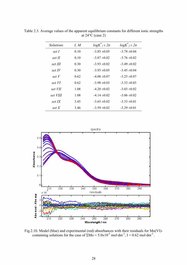
The attempts to fit a chosen model to the experimental data for the highest ionic
strength solutions (3.45 mol·dm-3 and 3.46 mol·dm-3) did not give good results despite the
very low confidence interval obtained. Firstly, negative values for molar absorptivity were
generated which do not have any physical meaning. Secondly, the discrepancy between the
model and experimental absorbances was very high (up to 0.1 in absorbance units) while for
all other cases, this difference did not exceed 0.004 absorbance units. (see fig. 2.10 as an
example). These facts along with previously discussed observations (e.g. figures 2.6e and
2.9c) show that determining ionisation constants of molybdic acid with the available model
is not feasible and that the forth species (most probably one of the polyanions) should be
considered in the speciation model.

24
a) b)
210 220 230 240 250 260 270 280 290 300
-0.3
-0.25
-0.2
-0.15
-0.1
-0.05
0
0.05
0.1
0.15
Wavelength / nm
UxS
1
2
3
210 220 230 240 250 260 270 280 290
-0.2
-0.15
-0.1
-0.05
0
0.05
0.1
0.15
0.2
0.25
0.3
Wavelength / nm
UxS
1
2
3
c) d)
210 220 230 240 250 260 270 280 290 300
-0.6
-0.5
-0.4
-0.3
-0.2
-0.1
0
0.1
0.2
0.3
Wavelength / nm
UxS
1
3
2
210 220 230 240 250 260 270 280 290
-0.1
0
0.1
0.2
0.3
0.4
Wavelength / nm
UxS
3
2
1
e)
210 220 230 240 250 260 270 280 290 300
-0.2
-0.1
0
0.1
0.2
0.3
0.4
Wavelength / nm
UxS
1
2
3
4?
Fig.2.6. Contribution of most significant vectors in total absorbance: (a) ΣMo = 5.2x10⁻⁵ mol·dm-3, I = 0.10 mol·dm-3; (b) ΣMo = 5.0x10⁻⁵ mol·dm-3, I = 0.30 mol·dm-3; (c) ΣMo = 5.0x10⁻⁵ mol·dm-3, I = 0.62 mol·dm-3; (d) ΣMo = 5.0x10⁻⁵ mol·dm-3, I = 1.08 mol·dm-3; (e) ΣMo = 4.2x10⁻⁵ mol·dm-3, I = 3.46 mol·dm-3

25
a)
210 220 230 240 250 260 270 280 2900
0.1
0.2
0.3
0.4
0.5
Wavelength / nm
Abs
orba
nce
5.264.984.724.594.384.274.214.093.953.773.543.333.183.02
pH=5.26
3.02
pH=5.26
3.02
pH
b)
210 220 230 240 250 260 270 280 290 3000
0.1
0.2
0.3
0.4
0.5
Wavelength / nm
Abs
orba
nce
5.204.904.664.524.464.344.214.164.053.923.743.553.373.183.02.842.35
pHpH=5.20
2.35
pH=5.20
2.35
Fig.2.7. Spectra of Mo(VI)-containing solutions at 24°C. (a) ΣMo = 5.2x10⁻⁵ mol·dm-3, I = 0.10 mol·dm-3; (b) ΣMo = 5.0x10⁻⁵ mol·dm-3, I = 0.62 mol·dm-3.

26
200 220 240 260 280 300
2000
4000
6000
8000
10000
12000
Wavelength /nm
Nor
mal
ised
abs
orba
nce
4.644.514.424.304.174.134.013.893.723.553.373.182.992.822.352.05
pHpH=4.64
2.05
pH=4.64 2.05
Fig.2.8. Normalized absorbance of Mo(VI)-containing solutions at 24°C.
ΣMo = 5.0x10⁻⁵ mol·dm-3, I = 1.08 mol·dm-3 .

27
a)
200
250
300
350
-200
00
2000
4000
6000
8000
1000
0
1200
0
Wav
ele
ng
th/
nm
Normalizedabsorbance
0.1
0M
0.6
2M
b)
200
250
300
350
-200
00
2000
4000
6000
8000
1000
0
1200
0
Wav
elen
gth
/nm
Normalizedabsorbance
0.10
M1.
08M
c)
200
250
300
350
-200
00
2000
4000
6000
8000
1000
0
1200
0
1400
0
Wa
ve
len
gth
/n
m
Normalizedabsorbance
0.1
0M
3.4
6M
Fig.
2.9.
Spec
tra(n
orm
aliz
edab
sorb
ance
)of
Mo-
cont
aini
ngso
lutio
nsat
diff
eren
tion
icst
reng
thsh
own
aton
efig
ure,
inbl
ack
the
low
erio
nic
stre
ngth
issh
own:
(a)
0.10
mol
·dm
-3
and
0.62
mol
·dm
-3;
(b)
0.10
mol
·dm
-3an
d1.
08m
ol·d
m-3
;(c
)0.1
0m
ol·d
m-3
and
3.46
mol
·dm
-3.
28
Table 2.3. Average values of the apparent equilibrium constants for different ionic strengths at 24°C (case 2)
Solutions I, M logK*
1 ± 2σ logK*2 ± 2σ
set I 0.10 -3.85 ±0.05 -3.78 ±0.04
set II 0.10 -3.87 ±0.02 -3.76 ±0.02
set III 0.30 -3.93 ±0.02 -3.49 ±0.02
set IV 0.30 -3.93 ±0.05 -3.45 ±0.04
set V 0.62 -4.08 ±0.07 -3.25 ±0.07
set VI 0.62 -3.98 ±0.03 -3.33 ±0.03
set VII 1.08 -4.20 ±0.02 -3.03 ±0.02
set VIII 1.08 -4.14 ±0.02 -3.06 ±0.02
set IX 3.45 -3.65 ±0.02 -3.33 ±0.01
set X 3.46 -3.59 ±0.02 -3.29 ±0.01
Fig.2.10. Model (blue) and experimental (red) absorbances with their residuals for Mo(VI)- containing solutions for the case of ΣMo = 5.0x10⁻⁵ mol·dm-3, I = 0.62 mol·dm-3 .

29
2.4.3. Case 3. pH buffered solutions at different (constant) ionic strength.
Because the two equilibrium constants are numerically very close to each other,
their reliable determination is difficult and therefore requires extreme preciseness in
preparing solutions. With this in mind, we decided to buffer pH (with acetate buffer) in order
to avoid small fluctuations in proton concentrations during the experiment which might
cause errors in the resulting values of the two equilibrium constants. Since it was shown that
at I = 3.45 mol·dm-3, there was probably a fourth species present which was incompatible
with our model, a series of the solutions having ionic strengths, 0.10 , 0.28, 0.56, 0.90
mol·dm-3 as well as a series with unadjusted ionic strength (i.e.varying, ≤0.005 mol·dm-3)
were prepared (Appendix 2.7.3). The maximum total molybdenum concentration was always
below the mononuclear wall (i.e.< 1x10⁻⁴ mol·dm-3). In addition, solutions with pH<2.5 were
also prepared in order to be able to define/study the equilibrium between the H2MoO4 and
H3MoO4+ species.
For the very acidic solutions, the absence of polynuclear species was also
confirmed at different ionic strengths by measuring spectra immediately after preparation
over a period of several hours (fig.2.11 a-d). If polynuclear species were formed at such
concentrations of total Mo and HClO4, an observable change in the spectra due to the slow
kinetics of forming such species (TYTKO and GLEMSER, 1976) would occur during this time.
In our case, absorbance at a given wavelength vs. time remains constant within instrumental
error. Several wavelengths were chosen for analysis (i.e. 200, 220, 260 nm where the
solutions absorb and at 320 nm where the solution does not absorb, as a reference). Such a
test was carried out for several solutions with different total concentrations of NaClO4. In all
the solutions, we confirmed that no change occurred with the time, indicating that no
polynuclear species were formed.
The method of the data treatment was the same as that described above for case 1
and 2. First, the number of absorbing species was established. In fig.2.12, one can see the
product of U and S matrices (result of SVD decomposition of absorbance matrix) plotted
versus wavelength, indicating the contribution of the most significant vectors to the
absorption profile. For each experiment, four curves (i.e. species) were distinguished, two of
which have significant contribution to the total absorbance, and two others whose
contribution is small. Therefore, it was concluded, that 4 absorbing species contribute to the
experimental spectra. Spectra of molybdate containing solutions for two different ionic
strengths are shown in the fig.2.13

30
200
220
240
260
280
300
320
340
360
380
0
0.050.
1
0.150.
2
0.250.
3
0.35
Wav
elen
gth
/n
m
Absorbance
050
0100
0150
03
3.54
4.55
x1
0-3
time
/min
Abs
32
0n
m
050
0100
015
00
0.0
59
0.0
6
0.0
61
0.0
62
0.0
63
time
/min
Abs
260n
m
05
00
100
0150
00
.34
8
0.3
49
0.3
5
0.3
51
0.3
52
time
/min
Abs
220n
m
050
0100
015
00
0.2
03
0.2
04
0.2
05
0.2
06
0.2
07
0.2
08
time
/min
Abs
200n
m
220
240
260
280
300
320
340
360
0
0.050.
1
0.150.
2
0.250.
3
Wav
elen
gth
/nm
Absorbance
05
01
00
2
2.2
2.4
2.6
2.8
x1
0-3
time
/min
Abs
320n
m
05
010
0
0.0
708
0.0
71
0.0
712
0.0
714
time
/min
Abs
260n
m
05
01
00
0.2
54
4
0.2
54
6
0.2
54
8
0.2
55
0.2
55
2
0.2
55
4
time
/min
Abs
220n
m
05
010
00
.288
4
0.2
886
0.2
888
0.2
89
time
/min
Abs
200n
m
Fig.
2.11
(a-b
). Sp
ectra
of M
o(V
I) c
onta
inin
g so
lutio
ns w
ith d
iffer
ent p
H a
nd a
t diff
eren
t ion
ic st
reng
th a
t 22°
C a
nd th
e pl
ots o
f val
ues o
fab
sorb
ance
vers
usw
avel
engt
h:(a
)ΣM
o =
5.7x
10-5
mol
·dm
-3,I
=n/a
(i.e.≤0
.005
mol
·dm
-3),
pH =
1.2
2;(b
)ΣM
o =
5.5x
10-5
mol
·dm
-3,I
=0.
10m
ol·d
m-3
,pH
=0.3
5.
b)a)

31
200
220
240
260
280
300
320
0
0.050.
1
0.150.
2
0.250.
3
0.35
Wav
elen
gth
/n
m
Absorbance
020
040
060
04
4.55
5.5
x10
-3
time/
min
Abs
320n
m
020
040
060
00.
083
0.08
4
0.08
5
0.08
6
time/
min
Abs
260n
m
020
040
060
00.
344
0.34
5
0.34
6
0.34
7
0.34
8
time/
min
Abs
220n
m
020
040
060
00.
36
0.36
1
0.36
2
0.36
3
0.36
4
0.36
5
time/
min
Abs
205n
m
220
240
260
280
300
320
340
360
0.4
0.5
0.6
0.7
0.8
0.91
Wav
elen
gth/
nm
Absorbance
010
020
030
00.
312
0.31
3
0.31
4
0.31
5
time/
min
Abs
320n
m
010
020
030
00.
325
0.32
6
0.32
7
0.32
8
0.32
9
time/
min
Abs
260n
m
010
020
030
00.
32
0.32
1
0.32
2
0.32
3
time/
min
Abs
220n
m
100
200
300
0.32
75
0.32
8
0.32
85
0.32
9
0.32
95
time/
min
Abs
205n
m
Fig.
2.11
(c-d
). Sp
ectra
of M
o(V
I) c
onta
inin
g so
lutio
ns w
ith d
iffer
ent p
H a
nd a
t diff
eren
t ion
ic st
reng
th a
t 22°
C a
nd th
e pl
ots o
f val
ues
of a
bsor
banc
e ve
rsus
wav
elen
gth:
(c)Σ
Mo
= 6.
55·1
0-5m
ol·d
m-3
,I= 0
.56
mol
·dm
-3 ,
pH=0
.58;
(d)Σ
Mo
= 6.
55·1
0-5m
ol·d
m-3
,I=
0.9
mol
·dm
-3, p
H=0
.85.
d)c)

32
a)
210 220 230 240 250 260 270 280 290
-0.1
-0.05
0
0.05
0.1
0.15
0.2
0.25
0.3
Wavelength / nm
UxS
1
2
3
4
b)
210 220 230 240 250 260 270 280 290
-0.1
-0.05
0
0.05
0.1
0.15
0.2
0.25
Wavelength / nm
UxS
1
2
3
4
c)
210 220 230 240 250 260 270 280 290
-0.1
-0.05
0
0.05
0.1
0.15
Wavelength / nm
UxS
1
2
3
4
d)
210 220 230 240 250 260 270 280 290 300
-0.2
-0.1
0
0.1
0.2
0.3
0.4
0.5
Wavelength / nm
UxS
1
4
2
3
Fig. 2.12. Contribution of most significant vectors in total absorbance: (a) ΣMo = 5.7·10-5 mol·dm-3, I=n/a (i.e. ≤0.005 mol·dm-3); (b) ΣMo = 5.8·10-5 mol·dm-3, I = 0.1 mol·dm-3;
(c) ΣMo = 5.5·10-5 mol·dm-3, I = 0.56 mol·dm-3; (d) ΣMo = 6.0·10-5 mol·dm-3, I = 0.9 mol·dm-3.

33
a)200 220 240 260 280 300 320 340
0
1000
2000
3000
4000
5000
6000
7000
8000
9000
10000
Wavelength / nm
Nor
mal
ized
Abs
orba
nce
0.360.670.981.191.491.782.062.272.512.853.193.553.704.064.214.464.714.955.205.50
pH=5.50
pH=0.36
pH
I= n/a[Mo tot]=5.7e-5M
pH=2.51
5.50 0.36
b)
200 220 240 260 280 3000
2000
4000
6000
8000
10000
Wavelength / nm
Nor
mal
ized
abs
orba
nce
0.680.861.051.311.651.922.212.402.652.953.263.553.643.964.084.334.584.835.085.40
pH
pH=5.40
pH=2.65
pH=0.68
pH=0.68pH=5.40
I=0.90M[Mo tot]=6e-5M
Fig. 2.13. Spectra (normalized absorbance) of Mo(VI) –containing solutions with buffered pH at 22 °C (a)Mo tot =5.7x10⁻⁵ mol·dm-3, I=n/a (i.e. ≤0.005 mol·dm-3);
(b) Mo tot =6.0x10⁻⁵ mol·dm-3, I=0.9 mol·dm-3.

34
Table 2.4. Values of the apparent equilibrium constants, logK*, at different ionic strengths at 22°C (case 3) obtained by different methods (see text); values in bold were held constant
during the optimisation calculations.
method logK *0 logK *
1 logK *2
I -0.98 -4.10 -4.08II -0.95 - -
IIIa -0.98 -4.10 -4.08IIIb -0.95 -4.11 -4.08IV -0.96 -4.11 -4.08V -0.96 -4.11 -4.08
method logK *0 logK *
1 logK *2
I -1.03 -3.92 -3.75II -0.93 - -
IIIa -1.03 -3.92 -3.75IIIb -0.93 -3.92 -3.75IV -1.03 -3.92 -3.75V -1.03 -3.91 -3.75
method logK *0 logK *
1 logK *2
I -1.01 -3.81 -3.55II -0.92 - -
IIIa -1.01 -3.81 -3.56IIIb -0.92 -3.82 -3.56IV -0.99 -3.82 -3.56V -1.01 -3.81 -3.56
method logK *0 logK *
1 logK *2
I -0.98 -3.84 -3.47II -0.97 - -
IIIa -0.98 -3.80 -3.46IIIb -0.97 -3.81 -3.46IV -0.97 -3.80 -3.46V -0.97 -3.80 -3.46
method logK *0 logK *
1 logK *2
I -0.90 -3.84 -3.34II -0.89 - -
IIIa -0.90 -3.83 -3.35IIIb -0.89 -3.83 -3.35IV -0.90 -3.83 -3.35V -0.90 -3.83 -3.35
set V
set I
set II
set III
set IV

35
For the calculation of the apparent equilibrium constants, K*0, K*
1 and K*2, several
approaches were applied (the calculation procedure itself was the same as described before
for the cases 1 and 2). The first approach (method I) was to optimize all three constants
simultaneously. The values of logK*0 were also obtained independently (method II) by
taking into account only the solutions in a very acidic interval where only two absorbing
species predominate (i.e. H3MoO4+ and H2MoO4). Both methods showed excellent
reproducibility between experimental and calculated spectra. In the method III, all the
solutions were included in the computation but only logK*1 and logK*
2 were optimised and
logK*0 was held constant at the value obtained using methods I and II (methods IIIa and IIIb
respectively). Method IV consisted of fixing logK*1 and logK*
2 (known from method I)
while logK*0 is being optimized. In method V, logK*
2 was fixed (known from method I) and
logK*0 and logK*
1 were optimized.
The results of the various optimization approaches are shown in the table 2.4. The
values in bold were fixed and were not optimized in method indicated. The various
optimisation approaches (methods I to V) all produced similar values of the equilibrium
constants, which confirms that simultaneous optimisation of all three constants yields
reliable values. One can see from the table that despite the differences in the initial values of
logK*0 for the solutions sets II and III, the values of logK*
1 and logK*2 obtained by method
III are the same, which indicates that the objective function is not “sharp” in the area of
minimum for the logK*0. In these cases, the error should be quite large, as confirmed by
calculated confidence interval (table 2.5). Table 2.5 gives the values of the three apparent
equilibrium constants, K*0 , K*
1 and K*2, which were optimised simultaneously.
Table 2.5. Average values of the apparent equilibrium constants at 22°C (case 3) together with the confidence intervals, obtained by Monte Carlo calculations with 10000 iterations.
Solutions I, M logK*
0 ± 2σ logK*1 ± 2σ logK*
2 ± 2σ
set I n/a -0.98 ±0.04 -4.10 ±0.03 -4.08 ±0.02
set II 0.10 -1.03 ±0.06 -3.92 ±0.03 -3.75 ±0.02
set III 0.28 -1.01 ±0.06 -3.81 ±0.03 -3.55 ±0.02
set IV 0.56 -0.98 ±0.04 -3.84 ±0.03 -3.47 ±0.02
set V 0.90 -0.90 ±0.03 -3.84±0.04 -3.34 ±0.03
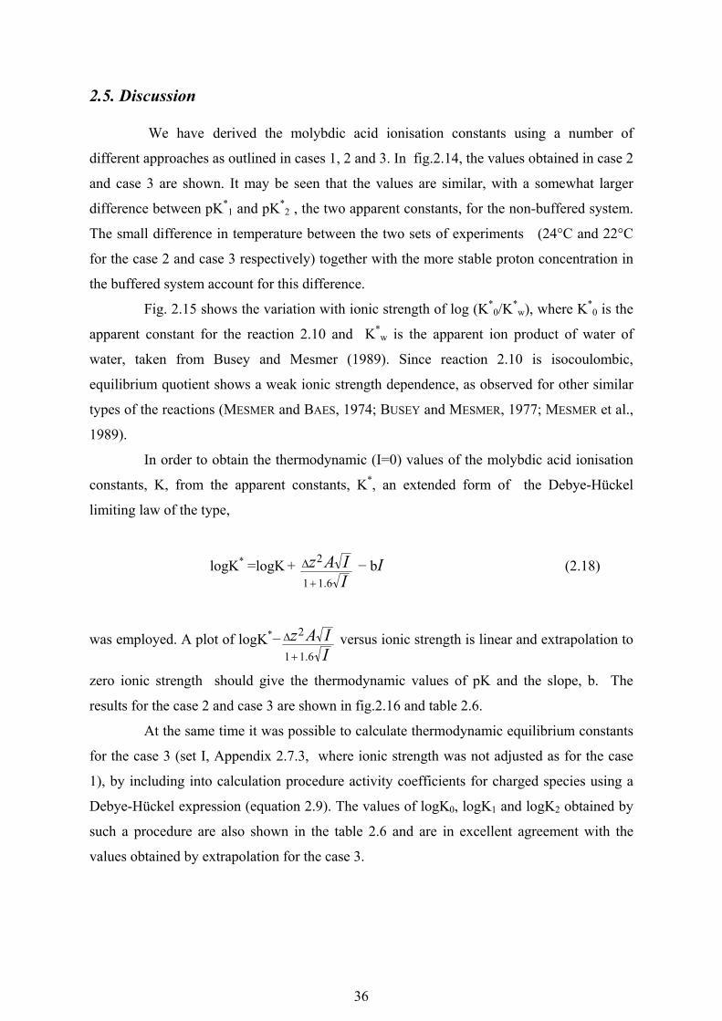
36
2.5. Discussion
We have derived the molybdic acid ionisation constants using a number of
different approaches as outlined in cases 1, 2 and 3. In fig.2.14, the values obtained in case 2
and case 3 are shown. It may be seen that the values are similar, with a somewhat larger
difference between pK*1 and pK*
2 , the two apparent constants, for the non-buffered system.
The small difference in temperature between the two sets of experiments (24°C and 22°C
for the case 2 and case 3 respectively) together with the more stable proton concentration in
the buffered system account for this difference.
Fig. 2.15 shows the variation with ionic strength of log (K*0/K*
w), where K*0 is the
apparent constant for the reaction 2.10 and K*w is the apparent ion product of water of
water, taken from Busey and Mesmer (1989). Since reaction 2.10 is isocoulombic,
equilibrium quotient shows a weak ionic strength dependence, as observed for other similar
types of the reactions (MESMER and BAES, 1974; BUSEY and MESMER, 1977; MESMER et al.,
1989).
In order to obtain the thermodynamic (I=0) values of the molybdic acid ionisation
constants, K, from the apparent constants, K*, an extended form of the Debye-Hückel
limiting law of the type,
logK* =logK + IIAz
6.11
2
+
Δ − bI (2.18)
was employed. A plot of logK*−IIAz
6.11
2
+
Δ versus ionic strength is linear and extrapolation to
zero ionic strength should give the thermodynamic values of pK and the slope, b. The
results for the case 2 and case 3 are shown in fig.2.16 and table 2.6.
At the same time it was possible to calculate thermodynamic equilibrium constants
for the case 3 (set I, Appendix 2.7.3, where ionic strength was not adjusted as for the case
1), by including into calculation procedure activity coefficients for charged species using a
Debye-Hückel expression (equation 2.9). The values of logK0, logK1 and logK2 obtained by
such a procedure are also shown in the table 2.6 and are in excellent agreement with the
values obtained by extrapolation for the case 3.

37
2.7
2.9
3.1
3.3
3.5
3.7
3.9
4.1
4.3
0.00 0.20 0.40 0.60 0.80 1.00 1.20 1.40
√I
pK*
pK1 (case 2)pK2 (case 2)pK1 (case 3)pK2 (case 3)
Fig. 2.14. The apparent equilibrium constants, pK*
1 and pK*2, at different ionic
strengths, obtained by analyzing non-buffered (case 2) and buffered (case 3) solutions.
11.50
12.00
12.50
13.00
13.50
14.00
0.00 0.10 0.20 0.30 0.40 0.50 0.60 0.70 0.80 0.90 1.00Ionic strength / M
log
(K*/
Kw
*)
Fig. 2.15. log(K*0/K*
w) as a function of ionic strength (see text).
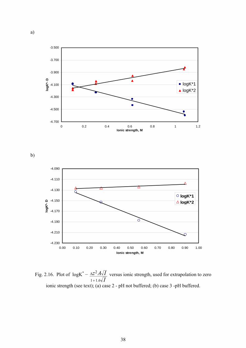
38
a)
-4.700
-4.500
-4.300
-4.100
-3.900
-3.700
-3.500
0 0.2 0.4 0.6 0.8 1 1.2Ionic strength, M
logK
*- D
logK*1logK*2
b)
-4.230
-4.210
-4.190
-4.170
-4.150
-4.130
-4.110
-4.090
0.00 0.10 0.20 0.30 0.40 0.50 0.60 0.70 0.80 0.90 1.00Ionic strength, M
logK
*- D
logK*1logK*2
Fig. 2.16. Plot of logK* −
IIAz
6.11
2
+
Δ versus ionic strength, used for extrapolation to zero
ionic strength (see text); (a) case 2 - pH not buffered; (b) case 3 -pH buffered.

39
Table 2.6. Values of logK0, logK1 and logK2 at zero ionic strength.
logK0 logK1 logK2
Calculated including activity coefficients ( I = unadjusted )
Case 1 (pH not buffered, 20°C) - -4.11 -4.10
Case 3 (pH buffered, 22°C, data set I) -0.99 -4.11 -4.12
Limiting law extrapolated ( I = constant )
Case 2 (pH not buffered, 24°C) - -4.06 -4.17
Case 3 (pH buffered, 22°C) -1.05 -4.12 -4.13
The distribution of Mo(VI) aqueous species in solution with total molybdenum
concentration of 5.70x10⁻⁵ mol·dm-3 as a function of pH at 22°C is shown in fig. 2.17. One
can see that monoprotonated species, HMoO4, never predominates and reaches maximum of
30% of total dissolved molybdate at pH ≈ 4. The H3MoO4+ species starts to become
significant at pH ≤ 2.5, which is consistent with the observations of Cruywagen (1989).
Absence of polynuclear species, buffered pH of the solution and advanced
mathematical treatment allows to consider the values of logK0 = -1.02, logK1= -4.12 and
logK2= -4.13 to be the best values for molybdic acid ionisation. This values were used to
calculate the molar absorptivities, ε, for each species as a function of wavelength. These are
shown in figure 2.18.

40
Fig. 2.17. Distribution diagram of Mo(VI) aqueous species in a solution at 22°C.
220 240 260 280 300 320 3400
1000
2000
3000
4000
5000
6000
7000
8000
9000
10000
Wavelength / nm
Mol
arab
sorp
tivi
ty
Fig. 2.18. Molar absorptivity for the Mo(VI) aqueous species.

41
2.6. References
Anany G. H., M. K.; Ismail, M. I. (1980) Spectrophotometric studies on molybdenum (VI and V) in absence and presence of phenols. Spectrochimica Acta, Part A: Molecular and Biomolecular Spectroscopy 36A(9), 853-857.
Aveston J., Anacker E. W., and Johnson J. S. (1964) Hydrolysis of molybdenum. VI. Ultracentrifugation, acidity measurements, and Raman spectra of polymolybdates. Inorg. Chem. 3(5), 735-46.
Bartecki A. D., Danuta. (1967) Spectroscopy of molybdenum(VI) compounds. Journal of Inorganic and Nuclear Chemistry 29 (12), 2907-2916.
Boily J.-F. and Suleimenov O. M. (2006) Extraction of Chemical Speciation and Molar Absorption Coefficients with Well-Posed Solutions of Beer's Law. Journal of Solution Chemistry 35(6), 917-926.
Brown P. L. S., Michael E.; Sylva, Ronald N. (1987) The hydrolysis of metal ions. Part 10. Kinetic and equilibrium measurements of molybdenum(VI). Journal of the Chemical Society, Dalton Transactions: Inorganic Chemistry (1972-1999) 9, 2149-2157.
Busey R. H. and Mesmer R. E. (1977) Ionization equilibriums of silicic acid and polysilicate formation in aqueous sodium chloride solutions to 300 DegC. Inorganic Chemistry 16(10), 2444-50.
Busey R. H. and Mesmer R. E. (1978) Thermodynamic quantities for the ionization of water in sodium chloride media to 300 DegC. Journal of Chemical and Engineering Data 23(2), 175-6.
Chojnacka J. (1963) Polarographic investigations on isopoly acids of molybdenum in solutions of HClO4. Zeszyty Nauk. Univ. Jagiel. Prace Chem. No. 8, 7-15.
Cruywagen J. J. and Rohwer E. F. C. H. (1975) Coordination number of molybdenum(VI) in monomeric molybdic acid. Inorganic Chemistry 14(12), 3136-7.
Cruywagen J. J., Heyns J. B. B., and Rohwer E. F. C. H. (1976) Spectrophotometric investigation of the protonation of monomeric molybdic acid in sodium perchlorate medium. Journal of Inorganic and Nuclear Chemistry 38(11), 2033-6.
Cruywagen J. J. and Heyns J. B. B. (1987) Equilibria and UV spectra of mono- and polynuclear molybdenum(VI) species. Inorganic Chemistry 26 (16), 2569-2572.
Cruywagen J. J. and Heyns J. B. B. (1989) Spectrophotometric determination of the thermodynamic parameters for the first two protonation reactions of molybdate: an advanced undergraduate laboratory experiment. Journal of Chemical Education 66(10), 861-863.
Cruywagen J. J. (2000) Protonation, oligomerization, and condensation reactions of vanadate(V), molybdate(VI), and tungstate(VI). Advances in Inorganic Chemistry 49, 127-182.
Farkas E., Csoka H., Micera G., and Dessi A. (1997) Copper(II), nickel(II), zinc(II), and molybdenum(VI) complexes of desferrioxamine B in aqueous solution. Journal of Inorganic Biochemistry 65(4), 281-286.
Fernandez D. P., Goodwin A. R. H., Lemmon E. W., Sengers J. M. H. L., and Williams R. C. (1997) A formulation for the static permittivity of water and steam at temperatures from 238 K to 873 K at pressures up to 1200 MPa, including derivatives and Debye-Hueckel coefficients. Journal of Physical and Chemical Reference Data 26(4), 1125-1166.
Ivanova G. F., Levkina N. I., Nesterova L. A., Zhidikova A. P., and Khodakovskii I. L. (1975) Equilibria in the molybdenum trioxide-water system in the 25-300°C range. Geokhimiya 2, 234-247.

42
Janz G. J., Oliver B. G., Lakshminarayanan G. R., and Mayer G. E. (1970) Electrical conductance, diffusion, viscosity, and density of sodium nitrate, sodium perchlorate, and sodium thiocyanate in concentrated aqueous solutions. Journal of Physical Chemistry 74(6), 1285-9.
Maksimova I. N., Pravdin N. N., and Razuvaev V. E. (1976) Study of hydrolysis of sodium chromate, molybdate, and tungstate in aqueous solutions at 15-90 Deg. Ukrainskii Khimicheskii Zhurnal (Russian Edition) 42(10), 1019-23.
Marshall W. L. and Franck E. U. (1981) Ion product of water substance, 0-1000°C, 1-10,000 bars, new international formulation and its background. Journal of Physical and Chemical Reference Data 10(2), 295-304.
Mesmer R. E. and Baes C. F., Jr. (1974) Phosphoric acid dissociation equilibriums in aqueous solutions to 300.deg. Journal of Solution Chemistry 3(4), 307-22.
Mesmer R. E., Patterson C. S., Busey R. H., and Holmes H. F. (1989) Ionization of acetic acid in aq. sodium chloride media: a potentiometric study to 573K and 130 bar. Journal of Physical Chemistry 93(21), 7483-90.
Minubayeva Z., Suleimenov O. M., and Seward T. M. (2008) Acridinium ion ionisation at elevated temperatures and pressures to 200°C and 2000 bar. Journal of Solution Chemistry, in print.
Nabivanets B. I. (1968) Isoelectric point of molybdic acid. Zhurnal Neorganicheskoi Khimii 13(3), 900-2.
Nazarenko V. A. and Shelikhina E. I. (1971) Spectrophotometric determination of formation constants for mononuclear hydroxo complexes of molybdenum(VI). Zhurnal Neorganicheskoi Khimii 16(1), 166-71.
Ozeki T., Hiroshi K., and Ikeda S. (1988) Study of equilibria in 0.03 mM molybdate acidic aqueous solutions by factor analysis applied to ultraviolet spectra. Analytical Chemistry 60(19), 2055-2059.
Ozeki T., Adachi H., and Ikeda S. (1991) New approach to estimate dissolved structure of ions in solution. Extraction of pure UV/visible spectrum using factor analysis and its simulation using MO calculation. Analytical Sciences 7(Suppl., Proc. Int. Congr. Anal. Sci., 1991, Pt. 1), 713-16.
Ozeki T. A., Hirohiko; Ikeda, Shigero. (1996) Estimation of the dissolved structures and condensation reactivities of mononuclear molybdenum(VI) species in solution using the UV-vis absorption spectra and molecular orbital calculation DV-Xa. Bulletin of the Chemical Society of Japan 69(3), 619-625.
Paffett M. T. and Anson F. C. (1981) Electrochemical generation of monomeric aquamolybdenum(V) by reduction of molybdenum(VI) at high dilution in trifluoromethanesulfonic acid. Inorganic Chemistry 20(11), 3967-72.
Pungor E. and Halasz A. (1970) Spectrophotometric examination of the isopolyacid of molybdenum. Journal of Inorganic and Nuclear Chemistry 32(4), 1187-97.
Sasaki Y., Lindqvist I., and Sillen L. G. (1959) First equilibrium steps in acidification of molybdate ion. Journal of Inorganic and Nuclear Chemistry 9, 93-4.
Sasaki Y. and Sillen L. G. (1964) Equilibriums in polymolybdate solutions. Acta Chemica Scandinavica 18(4), 1014.
Schwarzenbach G. and Meier J. (1958) Formation and investigation of unstable protonation and deprotonation products of complexes in aqueous solution. Journal of Inorganic and Nuclear Chemistry 8, 302-12.
Shock E. L. and Koretsky C. M. (1993) Metal-organic complexes in geochemical processes: calculation of standard partial molal thermodynamic properties of aqueous acetate complexes at high pressures and temperatures. Geochimica et Cosmochimica Acta 57(20), 4899-922.

43
Tossell J. A. (2005) Boric acid, \"carbonic\" acid, and N-containing oxyacids in aqueous solution: Ab initio studies of structure, pKa, NMR shifts, and isotopic fractionations. Geochimica et Cosmochimica Acta 69(24), 5647-5658.
Tytko K. H. and Glemser O. (1976) Isopolymolybdates and isopolytungstates. Advances in Inorganic Chemistry and Radiochemistry 19, 239-315.
Tytko K. H., Baethe G., and Cruywagen J. J. (1985) Equilibrium studies of aqueous polymolybdate solutions in 1 M sodium chloride medium at 25°C. Inorganic Chemistry 24(20), 3132-3136.
Tytko K. H. (1986) Structure, bonding and acid-base properties of protonated monometalate ions and polymetalate ions forming chains or rings of corner-sharing MO4 tetrahedra of transition metals of Groups V and VI. A theoretical approach. Polyhedron 5(1-2), 497-503.
Vorob'ev S. P., Davydov I. P., and Shilin I. V. (1967) Behavior of molybdenum(VI) in perchloric and nitric acid solutions. Zhurnal Neorganicheskoi Khimii 12(8), 2142-7.
Wagner W. (1998) Properties of Water and Steam/The Industrial Standard IAPWS-IF97 for the Thermodynamic Properties and Supplementary Equations for Other Properties.
Yagasaki A., Andersson I., and Pettersson L. (1987) Multicomponent polyanions. 41. Potentiometric and phosphorus-31 NMR study of equilibria in the molybdophenylphosphonate system in 0.6 M sodium (chloride) medium. Inorganic Chemistry 26(23), 3926-33.

44
2.7. Apendix
Apendix 2.7.1. Initial composition of the solutions (molal scale) for the case 1 (ionic strength not adjusted)
Mo tot Na tot HClO4 pH Mo tot Na tot HClO4 pHsol1 9.80E-06 1.96E-05 5.08E-06 5.36 sol1 2.12E-05 4.23E-05 4.98E-06 5.40sol2 9.73E-06 1.95E-05 1.00E-05 5.07 sol2 2.10E-05 4.20E-05 1.03E-05 5.09sol3 9.62E-06 1.92E-05 1.85E-05 4.80 sol3 2.08E-05 4.16E-05 1.84E-05 4.85sol4 9.55E-06 1.91E-05 2.44E-05 4.68 sol4 2.06E-05 4.12E-05 2.52E-05 4.71sol5 9.84E-06 1.97E-05 3.96E-05 4.47 sol5 2.13E-05 4.25E-05 4.26E-05 4.49sol6 9.84E-06 1.97E-05 4.84E-05 4.38 sol6 2.13E-05 4.25E-05 4.90E-05 4.43sol7 9.83E-06 1.97E-05 6.59E-05 4.24 sol7 2.12E-05 4.25E-05 6.38E-05 4.32sol8 9.82E-06 1.96E-05 7.58E-05 4.18 sol8 2.12E-05 4.25E-05 7.23E-05 4.26sol9 9.81E-06 1.96E-05 9.91E-05 4.05 sol9 2.12E-05 4.24E-05 1.02E-04 4.10
sol10 9.79E-06 1.96E-05 1.37E-04 3.90 sol10 2.12E-05 4.23E-05 1.37E-04 3.96sol11 9.76E-06 1.95E-05 2.03E-04 3.72 sol11 2.11E-05 4.22E-05 1.96E-04 3.78sol12 9.72E-06 1.94E-05 2.98E-04 3.55 sol12 2.10E-05 4.20E-05 2.98E-04 3.58sol13 9.65E-06 1.93E-05 4.44E-04 3.37 sol13 2.08E-05 4.17E-05 4.47E-04 3.39sol14 9.54E-06 1.91E-05 6.68E-04 3.19 sol14 2.06E-05 4.12E-05 6.57E-04 3.21sol15 9.39E-06 1.88E-05 9.69E-04 3.02 sol15 2.03E-05 4.06E-05 9.59E-04 3.04sol16 9.79E-06 1.96E-05 3.20E-03 2.50 sol16 2.12E-05 4.23E-05 3.34E-03 2.48
Mo tot Na tot HClO4 pH Mo tot Na tot HClO4 pHsol1 3.96E-05 7.92E-05 1.01E-05 5.25 sol1 4.05E-05 8.09E-05 6.68E-06 5.33sol2 3.92E-05 7.84E-05 1.77E-05 5.01 sol2 4.02E-05 8.04E-05 1.40E-05 5.02sol3 3.88E-05 7.77E-05 2.46E-05 4.86 sol3 3.98E-05 7.95E-05 2.48E-05 4.78sol4 4.00E-05 8.01E-05 3.96E-05 4.65 sol4 3.94E-05 7.89E-05 3.37E-05 4.65sol5 4.00E-05 8.00E-05 4.73E-05 4.57 sol5 4.06E-05 8.13E-05 4.41E-05 4.54sol6 4.00E-05 8.00E-05 6.38E-05 4.43 sol6 4.06E-05 8.13E-05 5.34E-05 4.46sol7 4.00E-05 7.99E-05 7.63E-05 4.35 sol7 4.06E-05 8.12E-05 7.27E-05 4.32sol8 3.99E-05 7.98E-05 9.81E-05 4.22 sol8 4.06E-05 8.12E-05 7.94E-05 4.28sol9 3.99E-05 7.97E-05 1.29E-04 4.08 sol9 4.05E-05 8.11E-05 1.11E-04 4.13
sol10 3.97E-05 7.94E-05 1.99E-04 3.85 sol10 4.05E-05 8.09E-05 1.48E-04 3.99sol11 3.95E-05 7.91E-05 2.98E-04 3.63 sol11 4.03E-05 8.07E-05 2.24E-04 3.78sol12 3.92E-05 7.85E-05 4.47E-04 3.42 sol12 4.01E-05 8.03E-05 3.39E-04 3.57sol13 3.88E-05 7.77E-05 6.47E-04 3.24 sol13 3.94E-05 7.88E-05 7.44E-04 3.17sol14 3.82E-05 7.64E-05 9.63E-04 3.05 sol14 3.88E-05 7.76E-05 1.10E-03 2.99sol15 3.99E-05 7.97E-05 3.08E-03 2.52 sol15 4.05E-05 8.09E-05 3.04E-03 2.53
Mo tot Na tot HClO4 pH Mo tot Na tot HClO4 pHsol1 4.07E-05 8.14E-05 6.85E-06 5.35 sol1 4.05E-05 8.09E-05 6.92E-06 5.34sol2 4.04E-05 8.08E-05 1.38E-05 5.05 sol2 4.02E-05 8.04E-05 1.40E-05 5.04sol3 4.00E-05 8.00E-05 2.51E-05 4.80 sol3 3.98E-05 7.95E-05 2.50E-05 4.79sol4 3.96E-05 7.93E-05 3.42E-05 4.67 sol4 3.94E-05 7.88E-05 3.45E-05 4.65sol5 4.09E-05 8.18E-05 4.64E-05 4.54 sol5 4.07E-05 8.13E-05 4.51E-05 4.54sol6 4.09E-05 8.17E-05 5.45E-05 4.47 sol6 4.06E-05 8.13E-05 5.40E-05 4.46sol7 4.08E-05 8.16E-05 7.73E-05 4.32 sol7 4.06E-05 8.12E-05 7.35E-05 4.32sol8 4.08E-05 8.16E-05 8.76E-05 4.26 sol8 4.06E-05 8.12E-05 8.69E-05 4.25sol9 4.08E-05 8.15E-05 1.12E-04 4.14 sol9 4.05E-05 8.11E-05 1.11E-04 4.13
sol10 4.07E-05 8.14E-05 1.48E-04 4.00 sol10 4.05E-05 8.09E-05 1.48E-04 3.99sol11 4.06E-05 8.11E-05 2.24E-04 3.79 sol11 4.03E-05 8.07E-05 2.27E-04 3.77sol12 4.04E-05 8.07E-05 3.40E-04 3.57 sol12 4.01E-05 8.03E-05 3.39E-04 3.56sol13 4.01E-05 8.01E-05 5.09E-04 3.36 sol13 3.98E-05 7.97E-05 5.07E-04 3.36sol14 3.97E-05 7.94E-05 7.20E-04 3.19 sol14 3.94E-05 7.88E-05 7.45E-04 3.17sol15 3.90E-05 7.80E-05 1.10E-03 2.99 sol15 3.88E-05 7.76E-05 1.10E-03 2.99sol16 4.07E-05 8.14E-05 3.07E-03 2.52 sol16 4.05E-05 8.09E-05 3.07E-03 2.52
set IV set V
set VI
set I set II
set III

45
Mo tot Na tot HClO4 pH Mo tot Na tot HClO4 pHsol1 1.00E-05 2.01E-05 6.95E-06 5.20 sol1 1.00E-05 2.01E-05 6.94E-06 5.20sol2 9.97E-06 1.99E-05 1.37E-05 4.91 sol2 9.97E-06 1.99E-05 1.43E-05 4.89sol3 9.87E-06 1.97E-05 2.49E-05 4.65 sol3 9.85E-06 1.97E-05 2.69E-05 4.62sol4 9.78E-06 1.96E-05 3.42E-05 4.51 sol4 9.77E-06 1.95E-05 3.49E-05 4.51sol5 1.01E-05 2.02E-05 4.15E-05 4.43 sol5 1.01E-05 2.02E-05 4.38E-05 4.41sol6 1.01E-05 2.02E-05 5.25E-05 4.33 sol6 1.01E-05 2.02E-05 5.62E-05 4.30sol7 1.01E-05 2.01E-05 6.98E-05 4.20 sol7 1.01E-05 2.01E-05 7.12E-05 4.20sol8 1.01E-05 2.01E-05 8.28E-05 4.13 sol8 1.01E-05 2.01E-05 8.35E-05 4.13sol9 1.01E-05 2.01E-05 1.16E-04 3.97 sol9 1.01E-05 2.01E-05 1.10E-04 4.00
sol10 1.00E-05 2.01E-05 1.51E-04 3.86 sol10 1.00E-05 2.01E-05 1.39E-04 3.90sol11 1.00E-05 2.00E-05 2.23E-04 3.68 sol11 1.00E-05 2.00E-05 2.28E-04 3.67sol12 9.96E-06 1.99E-05 3.38E-04 3.49 sol12 9.96E-06 1.99E-05 3.39E-04 3.49sol13 9.88E-06 1.98E-05 5.08E-04 3.31 sol13 9.88E-06 1.98E-05 5.09E-04 3.31sol14 9.78E-06 1.96E-05 7.44E-04 3.14 sol14 9.78E-06 1.96E-05 7.45E-04 3.14sol15 9.62E-06 1.92E-05 1.10E-03 2.96 sol15 9.62E-06 1.92E-05 1.10E-03 2.96sol16 1.00E-05 2.01E-05 3.09E-03 2.51 sol16 1.00E-05 2.01E-05 3.02E-03 2.52
Mo tot Na tot HClO4 pH Mo tot Na tot HClO4 pHsol1 4.05E-05 8.09E-05 6.41E-06 5.39 sol1 1.10E-04 2.19E-04 6.75E-06 5.48sol2 4.02E-05 8.04E-05 1.30E-05 5.09 sol2 1.08E-04 2.16E-04 1.39E-05 5.17sol3 3.98E-05 7.95E-05 2.32E-05 4.84 sol3 1.07E-04 2.14E-04 2.51E-05 4.93sol4 3.94E-05 7.88E-05 3.24E-05 4.69 sol4 1.06E-04 2.12E-04 3.45E-05 4.80sol5 4.06E-05 8.13E-05 4.41E-05 4.56 sol5 1.09E-04 2.19E-04 4.37E-05 4.71sol6 4.06E-05 8.13E-05 5.34E-05 4.48 sol6 1.09E-04 2.19E-04 5.34E-05 4.62sol7 4.06E-05 8.12E-05 7.27E-05 4.34 sol7 1.09E-04 2.18E-04 7.37E-05 4.49sol8 4.06E-05 8.12E-05 7.94E-05 4.30 sol8 1.09E-04 2.18E-04 8.17E-05 4.45sol9 4.05E-05 8.11E-05 1.11E-04 4.14 sol9 1.09E-04 2.18E-04 1.09E-04 4.32
sol10 4.05E-05 8.09E-05 1.48E-04 4.00 sol10 1.09E-04 2.18E-04 1.48E-04 4.19sol11 4.03E-05 8.07E-05 2.24E-04 3.78 sol11 1.09E-04 2.17E-04 2.17E-04 4.00sol12 4.01E-05 8.03E-05 3.39E-04 3.57 sol12 1.08E-04 2.16E-04 3.36E-04 3.74sol13 3.98E-05 7.97E-05 5.03E-04 3.37 sol13 1.07E-04 2.14E-04 5.09E-04 3.49sol14 3.94E-05 7.88E-05 7.44E-04 3.17 sol14 1.06E-04 2.12E-04 7.45E-04 3.26sol15 3.88E-05 7.76E-05 1.10E-03 2.99 sol15 1.05E-04 2.09E-04 1.07E-03 3.06sol16 4.05E-05 8.09E-05 3.04E-03 2.53 sol16 1.09E-04 2.18E-04 3.08E-03 2.54
set X
set VII set VIII
set IX
End of Appendix 2.7.1.

46
Apendix 2.7.2. Initial composition (molal scale) of the solutions for the case2 (adjusted ionic strength)
Mo tot HClO4 NaClO4 pH Mo tot HClO4 NaClO4 pHsol1 5.26E-05 7.28E-06 0.100 5.26 sol1 5.02E-05 6.91E-06 0.310 5.22sol2 5.22E-05 1.39E-05 0.100 4.98 sol2 4.99E-05 1.36E-05 0.308 4.93sol3 5.16E-05 2.57E-05 0.098 4.72 sol3 4.94E-05 2.44E-05 0.305 4.68sol4 5.12E-05 3.46E-05 0.098 4.59 sol4 4.89E-05 3.38E-05 0.303 4.54sol5 5.28E-05 4.09E-05 0.101 4.52 sol5 5.04E-05 3.87E-05 0.312 4.49sol6 5.28E-05 5.73E-05 0.101 4.38 sol6 5.04E-05 5.61E-05 0.312 4.33sol7 5.28E-05 7.44E-05 0.101 4.27 sol7 5.03E-05 7.64E-05 0.311 4.20sol8 5.27E-05 8.52E-05 0.101 4.21 sol8 5.03E-05 8.05E-05 0.311 4.18sol9 5.27E-05 1.10E-04 0.100 4.10 sol9 5.03E-05 1.11E-04 0.311 4.04
sol10 5.26E-05 1.52E-04 0.100 3.95 sol10 5.02E-05 1.45E-04 0.311 3.93sol11 5.24E-05 2.24E-04 0.100 3.77 sol11 5.00E-05 2.21E-04 0.309 3.75sol12 5.21E-05 3.56E-04 0.099 3.54 sol12 4.98E-05 3.30E-04 0.308 3.56sol13 5.17E-05 5.50E-04 0.099 3.33 sol13 4.94E-05 4.94E-04 0.306 3.37sol14 5.12E-05 7.42E-04 0.098 3.18 sol14 4.89E-05 7.28E-04 0.303 3.18sol15 5.05E-05 1.05E-03 0.096 3.02 sol15 4.82E-05 1.08E-03 0.298 2.99sol16 5.26E-05 2.90E-03 0.100 2.55 sol16 5.02E-05 2.94E-03 0.310 2.54
Mo tot HClO4 NaClO4 pH Mo tot HClO4 NaClO4 pHsol1 4.48E-05 7.12E-06 0.101 5.25 sol1 5.03E-05 6.99E-06 0.310 5.20sol2 4.45E-05 1.39E-05 0.100 4.96 sol2 5.00E-05 1.36E-05 0.308 4.92sol3 4.40E-05 2.48E-05 0.099 4.71 sol3 4.95E-05 2.44E-05 0.305 4.67sol4 4.36E-05 3.43E-05 0.098 4.58 sol4 5.05E-05 3.91E-05 0.312 4.47sol5 4.50E-05 5.37E-05 0.101 4.39 sol5 5.05E-05 5.73E-05 0.312 4.31sol6 4.50E-05 6.92E-05 0.101 4.28 sol6 5.05E-05 7.41E-05 0.311 4.21sol7 4.49E-05 8.53E-05 0.101 4.19 sol7 5.04E-05 8.11E-05 0.311 4.17sol8 4.49E-05 1.10E-04 0.101 4.08 sol8 5.04E-05 1.14E-04 0.311 4.03sol9 4.48E-05 1.46E-04 0.101 3.95 sol9 5.03E-05 1.50E-04 0.310 3.91
sol10 4.47E-05 2.21E-04 0.101 3.76 sol10 5.01E-05 2.23E-04 0.309 3.74sol11 4.44E-05 3.36E-04 0.100 3.56 sol11 4.99E-05 3.34E-04 0.308 3.55sol12 4.41E-05 5.00E-04 0.099 3.37 sol12 4.95E-05 4.95E-04 0.306 3.37sol13 4.37E-05 7.39E-04 0.098 3.18 sol13 4.94E-05 5.58E-04 0.305 3.31sol14 4.30E-05 1.09E-03 0.097 2.99 sol14 4.83E-05 1.07E-03 0.298 3.00sol15 4.48E-05 2.98E-03 0.101 2.54 sol15 5.03E-05 2.88E-03 0.310 2.55
Mo tot HClO4 NaClO4 pH Mo tot HClO4 NaClO4 pHsol1 5.01E-05 6.63E-06 0.648 5.19 sol1 5.03E-05 6.52E-06 1.150 5.18sol2 4.98E-05 1.32E-05 0.644 4.90 sol2 5.00E-05 1.31E-05 1.143 4.88sol3 4.93E-05 2.38E-05 0.637 4.65 sol3 4.95E-05 2.34E-05 1.132 4.63sol4 4.88E-05 3.26E-05 0.632 4.52 sol4 4.91E-05 3.19E-05 1.122 4.50sol5 5.03E-05 3.78E-05 0.651 4.46 sol5 5.05E-05 4.10E-05 1.155 4.40sol6 5.03E-05 5.27E-05 0.650 4.32 sol6 5.05E-05 5.14E-05 1.155 4.30sol7 5.02E-05 7.45E-05 0.650 4.18 sol7 5.05E-05 7.00E-05 1.154 4.18sol8 5.02E-05 7.85E-05 0.650 4.15 sol8 5.04E-05 7.87E-05 1.153 4.13sol9 5.02E-05 1.09E-04 0.649 4.02 sol9 5.04E-05 1.05E-04 1.152 4.01
sol10 5.01E-05 1.49E-04 0.648 3.89 sol10 5.03E-05 1.46E-04 1.150 3.88sol11 4.99E-05 2.18E-04 0.646 3.73 sol11 5.02E-05 2.06E-04 1.147 3.73sol12 4.97E-05 3.20E-04 0.643 3.56 sol12 4.99E-05 3.20E-04 1.141 3.54sol13 4.93E-05 4.87E-04 0.638 3.36 sol13 4.95E-05 4.94E-04 1.133 3.34sol14 4.88E-05 7.14E-04 0.632 3.18 sol14 4.90E-05 7.35E-04 1.120 3.15sol15 4.82E-05 1.03E-03 0.623 3.01 sol15 4.84E-05 1.03E-03 1.106 2.99sol16 5.02E-05 1.50E-03 0.650 2.83 sol16 5.05E-05 1.36E-03 1.154 2.86sol17 4.99E-05 4.31E-03 0.646 2.36 sol17 5.01E-05 4.31E-03 1.146 2.34
set III (I=0.30 M)
set IV (I=0.30 M)
set VII (I=1.08 M)set V (I=0.62 M)
set I (I =0.10 M)
set II (I=0.10 M)

47
Mo tot HClO4 NaClO4 pH Mo tot HClO4 NaClO4 pHsol1 5.01E-05 6.81E-06 0.646 5.20 sol1 5.06E-05 6.57E-06 1.142 5.17sol2 4.98E-05 1.36E-05 0.642 4.90 sol2 5.03E-05 1.29E-05 1.135 4.88sol3 4.93E-05 2.38E-05 0.636 4.66 sol3 4.98E-05 2.31E-05 1.124 4.64sol4 4.89E-05 3.29E-05 0.630 4.53 sol4 4.94E-05 3.17E-05 1.114 4.50sol5 5.03E-05 3.81E-05 0.649 4.47 sol5 5.08E-05 3.89E-05 1.147 4.42sol6 5.03E-05 5.09E-05 0.649 4.34 sol6 5.08E-05 5.21E-05 1.146 4.29sol7 5.03E-05 7.01E-05 0.648 4.21 sol7 5.08E-05 7.14E-05 1.145 4.16sol8 5.02E-05 8.03E-05 0.648 4.16 sol8 5.07E-05 7.93E-05 1.145 4.12sol9 5.02E-05 1.06E-04 0.647 4.04 sol9 5.07E-05 1.05E-04 1.144 4.01
sol10 5.01E-05 1.42E-04 0.646 3.92 sol10 5.06E-05 1.42E-04 1.142 3.88sol11 5.00E-05 2.16E-04 0.644 3.74 sol11 5.05E-05 2.11E-04 1.138 3.72sol12 4.97E-05 3.24E-04 0.641 3.55 sol12 5.02E-05 3.11E-04 1.133 3.55sol13 4.94E-05 4.85E-04 0.637 3.37 sol13 4.99E-05 4.68E-04 1.126 3.36sol14 4.89E-05 7.12E-04 0.630 3.18 sol14 4.94E-05 6.91E-04 1.115 3.18sol15 4.82E-05 1.05E-03 0.621 3.00 sol15 4.87E-05 1.02E-03 1.098 3.00sol16 5.03E-05 1.48E-03 0.648 2.84 sol16 5.07E-05 1.49E-03 1.145 2.82sol17 4.99E-05 4.34E-03 0.644 2.35 sol17 5.04E-05 4.26E-03 1.138 2.35
Mo tot HClO4 NaClO4 pH Mo tot HClO4 NaClO4 pHsol1 4.18E-05 5.54E-06 4.155 5.19 sol1 4.19E-05 5.60E-06 4.158 5.19sol2 4.16E-05 1.11E-05 4.134 4.89 sol2 4.17E-05 1.14E-05 4.135 4.88sol3 4.12E-05 1.95E-05 4.101 4.65 sol3 4.14E-05 2.00E-05 4.102 4.64sol4 4.09E-05 2.75E-05 4.069 4.50 sol4 4.11E-05 2.75E-05 4.072 4.50sol5 4.19E-05 3.28E-05 4.171 4.42 sol5 4.21E-05 2.96E-05 4.174 4.47sol6 4.19E-05 4.52E-05 4.169 4.28 sol6 4.21E-05 4.62E-05 4.172 4.28sol7 4.19E-05 6.08E-05 4.166 4.16 sol7 4.20E-05 6.16E-05 4.169 4.15sol8 4.19E-05 6.87E-05 4.165 4.11 sol8 4.20E-05 6.97E-05 4.168 4.10sol9 4.18E-05 8.89E-05 4.161 4.00 sol9 4.20E-05 9.27E-05 4.164 3.98
sol10 4.18E-05 1.22E-04 4.155 3.86 sol10 4.19E-05 1.23E-04 4.158 3.86sol11 4.17E-05 1.84E-04 4.144 3.69 sol11 4.18E-05 1.76E-04 4.148 3.70sol12 4.15E-05 2.70E-04 4.129 3.52 sol12 4.17E-05 2.69E-04 4.132 3.52sol13 4.13E-05 4.03E-04 4.105 3.34 sol13 4.14E-05 4.03E-04 4.108 3.34sol14 4.09E-05 5.94E-04 4.070 3.17 sol14 4.08E-05 7.53E-04 4.045 3.06sol15 4.04E-05 8.76E-04 4.020 2.99 sol15 4.06E-05 8.82E-04 4.021 2.99sol16 4.19E-05 1.26E-03 4.166 2.83 sol16 4.21E-05 1.17E-03 4.170 2.86sol17 4.17E-05 3.65E-03 4.144 2.35 sol17 4.18E-05 3.72E-03 4.146 2.34
set X (I=3.46 M)
set VI (I=0.62 M)
set IX (I=3.45 M)
set VIII (I=1.08 M)
End of Appendix 2.7.2.

48
Apendix 2.7.3. Initial composition (molal scale) of the solutions for the case 3 (buffered pH, adjusted ionic strength)
CH3COOH CH3COONa HClO4 Mo tot CH3COOtot Na tot NaClO4 pHsol1 0 0 4.418E-01 5.468E-05 0 1.094E-04 0 0.46sol2 0 0 2.152E-01 5.489E-05 0 1.098E-04 0 0.76sol3 0 0 1.061E-01 5.387E-05 0 1.077E-04 0 1.06sol4 0 0 6.442E-02 5.595E-05 0 1.119E-04 0 1.26sol5 0 0 3.252E-02 5.766E-05 0 1.153E-04 0 1.55sol6 0 0 1.693E-02 5.955E-05 0 1.191E-04 0 1.82sol7 0 0 8.764E-03 5.733E-05 0 1.147E-04 0 2.10sol8 0 0 5.452E-03 5.797E-05 0 1.159E-04 0 2.29sol9 0 0 3.197E-03 5.573E-05 0 1.115E-04 0 2.52
sol10 0 0 1.514E-03 5.749E-05 0 1.150E-04 0 2.84sol11 0 0 7.494E-04 5.612E-05 0 1.122E-04 0 3.14sol12 0 0 3.796E-04 5.674E-05 0 1.135E-04 0 3.43sol13 3.262E-03 0 0 5.729E-05 3.262E-03 1.146E-04 0 3.64sol14 8.242E-04 0 0 5.769E-05 8.242E-04 1.154E-04 0 3.95sol15 3.267E-03 8.779E-04 0 5.670E-05 4.145E-03 9.913E-04 0 4.21sol16 1.788E-03 8.780E-04 0 5.652E-05 2.666E-03 9.910E-04 0 4.46sol17 9.821E-04 8.798E-04 0 5.936E-05 1.862E-03 9.985E-04 0 4.71sol18 7.370E-04 1.193E-03 0 5.720E-05 1.930E-03 1.307E-03 0 4.97sol19 4.227E-04 1.232E-03 0 5.932E-05 1.655E-03 1.351E-03 0 5.23sol20 1.812E-04 1.052E-03 0 6.082E-05 1.234E-03 1.174E-03 0 5.56
CH3COOH CH3COONa HClO4 Mo tot CH3COOtot Na tot NaClO4 pHsol1 0 0 1.864E-01 4.650E-05 0 9.299E-05 6.8E-02 0.83sol2 0 0 1.048E-01 5.079E-05 0 1.016E-04 8.1E-02 1.07sol3 0 0 6.605E-02 5.530E-05 0 1.106E-04 8.7E-02 1.27sol4 0 0 3.176E-02 5.751E-05 0 1.150E-04 9.2E-02 1.58sol5 0 0 1.600E-02 5.328E-05 0 1.066E-04 9.5E-02 1.88sol6 0 0 8.198E-03 5.496E-05 0 1.099E-04 9.6E-02 2.17sol7 0 0 5.319E-03 4.983E-05 0 9.967E-05 9.7E-02 2.36sol8 0 0 3.200E-03 5.845E-05 0 1.169E-04 9.6E-02 2.58sol9 0 0 1.459E-03 6.138E-05 0 1.228E-04 9.2E-02 2.92
sol10 0 0 7.753E-04 6.029E-05 0 1.206E-04 9.4E-02 3.19sol11 0 0 3.786E-04 5.904E-05 0 1.181E-04 9.5E-02 3.50sol12 3.232E-03 0 0 5.846E-05 3.232E-03 1.169E-04 9.5E-02 3.63sol13 8.147E-04 0 0 5.891E-05 8.147E-04 1.178E-04 9.6E-02 3.95sol14 3.232E-03 1.075E-03 0 6.187E-05 4.307E-03 1.199E-03 9.4E-02 4.21sol15 1.789E-03 8.728E-04 0 6.218E-05 2.662E-03 9.971E-04 9.5E-02 4.38sol16 9.764E-04 8.791E-04 0 6.056E-05 1.855E-03 1.000E-03 9.6E-02 4.63sol17 7.494E-04 1.234E-03 0 5.880E-05 1.984E-03 1.352E-03 9.6E-02 4.88sol18 3.957E-04 1.205E-03 0 5.827E-05 1.601E-03 1.321E-03 9.6E-02 5.15sol19 1.686E-04 1.011E-03 0 5.819E-05 1.179E-03 1.127E-03 9.6E-02 5.44
CH3COOH CH3COONa HClO4 Mo tot CH3COOtot Na tot NaClO4 pHsol1 0 0 1.914E-01 5.038E-05 0 1.008E-04 2.0E-01 0.82sol2 0 0 1.201E-01 5.868E-05 0 1.174E-04 2.3E-01 1.02sol3 0 0 5.477E-02 4.321E-05 0 8.643E-05 2.7E-01 1.36sol4 0 0 2.901E-02 4.959E-05 0 9.918E-05 2.8E-01 1.64sol5 0 0 1.651E-02 6.144E-05 0 1.229E-04 2.8E-01 1.88sol6 0 0 8.785E-03 6.075E-05 0 1.215E-04 2.8E-01 2.15sol7 0 0 5.453E-03 5.949E-05 0 1.190E-04 2.9E-01 2.36sol8 0 0 3.286E-03 5.506E-05 0 1.101E-04 2.9E-01 2.58sol9 0 0 1.522E-03 5.622E-05 0 1.124E-04 2.7E-01 2.92
sol10 0 0 7.428E-04 5.802E-05 0 1.160E-04 2.8E-01 3.23sol11 0 0 3.769E-04 5.986E-05 0 1.197E-04 2.9E-01 3.52sol12 5.973E-03 0 0 5.182E-05 5.973E-03 1.036E-04 2.8E-01 3.49sol13 8.168E-04 0 0 5.548E-05 8.168E-04 1.110E-04 2.9E-01 3.94sol14 3.273E-03 8.850E-04 0 5.940E-05 4.158E-03 1.004E-03 2.8E-01 4.11sol15 1.802E-03 8.847E-04 0 6.203E-05 2.686E-03 1.009E-03 2.8E-01 4.35sol16 9.972E-04 8.822E-04 0 5.896E-05 1.879E-03 1.000E-03 2.9E-01 4.59sol17 7.495E-04 1.251E-03 0 5.755E-05 2.000E-03 1.366E-03 2.9E-01 4.86sol18 4.198E-04 1.240E-03 0 6.055E-05 1.660E-03 1.361E-03 2.9E-01 5.10sol19 1.683E-04 1.066E-03 0 6.098E-05 1.234E-03 1.188E-03 2.9E-01 5.43
set I (I =n/a)
set III (I =0.28 M)
set II (I =0.10 M)

49
CH3COOH CH3COONa HClO4 Mo tot CH3COOtot Na tot NaClO4sol1 0 0 1.745E-01 5.375E-05 0 1.075E-04 4.2E-01 0.86sol2 0 0 1.026E-01 5.643E-05 0 1.129E-04 4.9E-01 1.04sol3 0 0 6.319E-02 5.877E-05 0 1.175E-04 5.2E-01 1.30sol4 0 0 3.233E-02 5.786E-05 0 1.157E-04 5.5E-01 1.58sol5 0 0 1.509E-02 5.388E-05 0 1.078E-04 5.7E-01 1.93sol6 0 0 8.505E-03 5.449E-05 0 1.090E-04 5.8E-01 2.18sol7 0 0 5.224E-03 5.493E-05 0 1.099E-04 5.8E-01 2.39sol8 0 0 3.117E-03 5.640E-05 0 1.128E-04 5.8E-01 2.61sol9 0 0 1.495E-03 5.873E-05 0 1.175E-04 5.5E-01 2.93
sol10 0 0 7.476E-04 5.514E-05 0 1.103E-04 5.7E-01 3.23sol11 0 0 3.698E-04 5.471E-05 0 1.094E-04 5.8E-01 3.54sol12 5.915E-03 0 0 5.146E-05 5.915E-03 1.029E-04 5.7E-01 3.48sol13 8.361E-04 0 0 5.692E-05 8.361E-04 1.138E-04 5.8E-01 3.93sol14 3.198E-03 8.693E-04 0 5.974E-05 4.067E-03 9.888E-04 5.7E-01 4.10sol15 1.788E-03 8.749E-04 0 5.844E-05 2.663E-03 9.917E-04 5.8E-01 4.33sol16 9.717E-04 8.839E-04 0 6.107E-05 1.856E-03 1.006E-03 5.8E-01 4.59sol17 7.461E-04 1.235E-03 0 6.238E-05 1.981E-03 1.359E-03 5.8E-01 4.84sol18 4.033E-04 1.232E-03 0 6.070E-05 1.635E-03 1.354E-03 5.8E-01 5.10sol19 1.609E-04 1.246E-03 0 5.938E-05 1.407E-03 1.365E-03 5.8E-01 5.50
CH3COOH CH3COONa HClO4 Mo tot CH3COOtot Na tot NaClO4 pHsol1 0 0 2.650E-01 6.545E-05 0 1.309E-04 5.3E-01 0.68sol2 0 0 1.775E-01 6.307E-05 0 1.261E-04 6.7E-01 0.86sol3 0 0 1.121E-01 6.127E-05 0 1.225E-04 7.8E-01 1.05sol4 0 0 6.176E-02 6.823E-05 0 1.365E-04 8.5E-01 1.31sol5 0 0 2.856E-02 6.346E-05 0 1.269E-04 9.1E-01 1.65sol6 0 0 1.536E-02 6.546E-05 0 1.309E-04 9.3E-01 1.92sol7 0 0 7.797E-03 6.499E-05 0 1.300E-04 9.4E-01 2.21sol8 0 0 5.004E-03 6.175E-05 0 1.235E-04 9.5E-01 2.40sol9 0 0 2.875E-03 6.402E-05 0 1.280E-04 9.5E-01 2.65
sol10 0 0 1.422E-03 6.204E-05 0 1.241E-04 9.1E-01 2.95sol11 0 0 7.051E-04 5.871E-05 0 1.174E-04 9.4E-01 3.26sol12 0 0 3.560E-04 5.718E-05 0 1.144E-04 9.5E-01 3.55sol13 2.876E-03 0 0 5.181E-05 2.876E-03 1.036E-04 9.5E-01 3.64sol14 7.363E-04 0 0 5.433E-05 7.363E-04 1.087E-04 9.6E-01 3.96sol15 3.070E-03 8.247E-04 0 5.734E-05 3.895E-03 9.394E-04 9.4E-01 4.08sol16 1.688E-03 8.295E-04 0 5.751E-05 2.517E-03 9.445E-04 9.5E-01 4.33sol17 9.223E-04 8.344E-04 0 5.456E-05 1.757E-03 9.436E-04 9.6E-01 4.58sol18 6.941E-04 1.162E-03 0 5.722E-05 1.856E-03 1.276E-03 9.5E-01 4.83sol19 3.920E-04 1.160E-03 0 5.778E-05 1.552E-03 1.275E-03 9.6E-01 5.08sol20 1.589E-04 9.920E-04 0 5.600E-05 1.151E-03 1.104E-03 9.6E-01 5.40
set IV (I =0.56 M)
set V (I =0.90 M)
End of Appendix 2.7.3.

50
3. Molybdic acid ionisation at elevated temperatures
3.1. Introduction A number of studies at elevated temperatures have been carried out on the
solubility of MoO2 (250-450°C) (KUDRIN, 1985), CaMoO4 and Na2MoO4 (25-300°C)
(ZHIDIKOVA and KHODAKOVSKII, 1971; ZHIDIKOVA et al., 1973), MoO2 and Na2MoO4 (25-
200°C) (IVANOVA et al., 1975), as well on hydrolysis of sodium molybdate (MAKSIMOVA et
al., 1976) in a 15-90°C range. The free energies of formation of sodium molybdate and
molybdate ion have also been determined by Graham and Hepler (1956) , Urusov et al.
(1967) and Zhidikova and Kuskov (1971). Ivanova et al. (1975) derives the empirical
equations for the temperature dependence of the first and second dissociation constants of
molybdic acid based on the assumption that ΔS°diss for the most of the acids have similar
values ( average of -79.496 J·mol-1·K-1 and -125.52 J·mol-1·K-1 for the first and second
dissociation step respectively). Arnorsson and Ivarsson (1985) applying electrostatic method
of Helgeson, propose their equation for the second ionisation constant of molybdic acid.
Nevertheless, there has been no previous systematic experimental study of the ionisation
equilibria of molybdic acid at elevated temperatures done and therefore no experimental data
for these reactions are available. Some data could be estimated from above mentioned
works, but the speciation of molybdic acid in aqueous solution is very much dependent on
the total molybdenum concentration (because of the formation of polyanions). The
composition of the solution (i.e. ionic strength) also can favour polymerisation (see previous
chapter).
This spectrophotometric study therefore is an attempt to obtain reliable
experimental thermodynamic data for the ionisation of molybdic acid at elevated
temperatures. Our experiments were aimed at determining the dependence of the first and
second dissociation constants of molybdic acid as a function of temperature (from 30 to
300°C) at the saturated water vapour pressure ( i.e. eq. 3.1 and 3.2 respectively).
++↔ HHMoOMoOH -4
042 (3.1)
+− +↔ HMoOHMoO 24
-4 (3.2)

51
3.2. Experimental method All solutions were prepared on a molal scale with Nanopure Millipore water
(resistivity >18MΩ/cm). Perchloric acid stock solution was diluted from concentrated acid
(HClO4, 60%, p.a., Merck) and standardized by colorimetric titration against dried Trisma-
base (Ttris(hydroxymethyl)aminomethane, 99+%, Aldrich) using methyl red as indicator and
potentiometric titration (using a glass combination electrode (Metrohm). Sodium hydroxide
solution was prepared from saturated sodium hydroxide solution (50% solution, Aldrich)
with CO2-free water and standardized under an argon pressure slightly above atmospheric
(in order to avoid CO2 absorption by NaOH solutions) by potentiometric and colorimetric
titration against standardized perchloric acid (using methyl red as an indicator). The water
was degassed under partial vacuum in an ultrasonic bath periodically purged with oxygen
free argon, which was obtained by passing argon (grade 4.8) through a column of copper
fillings at 425°C. The prepared solution was stored in a flask connected with a glass tube
filled with ascarite (Fluka, 5-20mesh) and drierite (Fluka, +4 mesh) in order to keep it CO2-
free. The pH of the studied solutions was maintained by various combinations of the above
mentioned reagents. pH was measured at atmospheric pressure and room temperature with
a glass combination electrode, calibrated every day against at least 2 standard buffer
solutions.
Sodium molybdate stock solutions (10-2 mol·dm-3) were prepared by dissolving
sodium molybdate dihydrate salt (99,99%, Aldrich) in nanopure Millipore water and kept in
a polyethylene bottle. All others solutions of sodium molybdate were prepared (by weight)
by dilution of stock solution.
A high-temperature flow-through spectrophotometric system (SULEIMENOV and
SEWARD, 2000) was used to conduct experiments at eight temperatures from 30 to 300°C.
The optical cell was made of titanium-palladium alloy provided with cylindrical 5mm thick
silica-glass windows in a screwed cup design. The solutions were pumped into the cell with
a HPLC pump (PrepStar, Varian) and purged of dissolved gases with an on-line vacuum
degassing system (Alltech). All the connection parts which were in contact with the solution
were made of PEEK® (including the head unit in HPLC pump) or Teflon®. The pressure was
monitored by a pressure module inside the HPLC pump and controlled by a back pressure
regulator (Upchurch Scientific High Pressure Adjustable BPR) and was maintained at 10-20
bars above the saturation water vapour pressure at each temperature.

52
The spectra were collected with a Varian Cary 5 double-beam spectrophotometer in
the 190-500 nm wavelength range at 0.5 nm intervals with a 100 nm/min scanning rate. All
spectra were corrected for background absorbance (windows+water+ClO4− and/or OH−).
Molar absorptivities of ClO4− or OH− were obtained from the spectra of HClO4 and NaOH
solutions, which were measured separately at the temperatures studied. Spectra of blank
solutions for all studied temperatures were taken before and after each solution. Three
consecutive spectra were taken for each solution at each temperature. The cell was flushed
with fresh solutions at each studied temperature to avoid the influence of any possible
decomposition products of perchloric acid at elevated temperatures with the time (ZINOV'EV
and BABAEVA, 1961; SWADDLE et al., 1971; SOLYMOSI, 1977; RATCLIFFE and IRISH, 1984).
Spectra were measured 15-20 minutes after the desired temperature was reached to allow the
temperature equilibration. The total concentration of molybdenum was low and ranged from
0.04 to 0.06 mmol·kg-1 (Appendix 3.6.1 and 3.6.2).
3.3. Data treatment The measured spectra (background corrected) were stored in an absorbance matrix,
Ai×j, where i=number of wavelengths, j = number of analysed solutions. In order to
determine the number of absorbing species (î.e. the rank or number of principal components)
required for a chemical model, we used a singular value decomposition (SVD) approach,
such that,
Ai×j = U i×n × S n×n × V j×n T (3.3)
where the matrixes U, S, V are the result of singular value decomposition of matrix A, U is
the i×n matrix of left singular vectors that form an orthonormal basis for the absorption
profile, S is the n×n diagonal matrix of singular values, and V is the n×j matrix of right
singular values, that form an orthonormal basis for the concentration dependence response.
By convention, the ordering of the singular vectors is determined by high-to-low sorting of
singular values, with the highest singular value in the upper left index of the matrix. One
important result of the singular value decomposition of A is that
A(l) =∑ U k × S k × V T k (3.4)
is the closest rank-l matrix to our original absorbance matrix Ai×j, (i.e. A(l) minimizes the
sum of the squares of the difference of the elements of A and A(l)) . In fig. 3.1, one can see
the product of U and S matrices plotted versus wavelength at each studied temperature,
indicating the contribution of the most significant vectors to the absorption profile. Such a

53
procedure demonstrated that for the temperatures from 30 to 100°C, three vectors (i.e. three
absorbing species, H2MoO4, HMoO4−and MoO4
2- ; model I) represent more than 99% of the
raw absorption data and all the rest are randomly oscillating around zero and therefore were
discarded, as most probably corresponding to random instrumental noise and small
imprecisions in solution preparation. At 150 and 200°C, the contribution of the third vector
is very small and the data treatment procedure was carried out using two hypotheses, one
considering three absorbing species (model I) and the other considering only two species
(i.e. HMoO4- and MoO4
2- species (model IIa), and H2MoO4 and MoO42- species (model
IIb)). For the case of 250°C, only two species were considered (i.e. model II) as indicated by
the contribution of the most significant vectors (fig.3.1).
After the number of absorbing species has been determined, the chemical model
can be ascribed as a system of seven linear equations which are as follows:
(i) the equilibrium deprotonation constants of molybdic acid (see equations 3.1 and 3.2) are,
[ ] [ ][ ]LH
HHLK HHL
21
+− ⋅⋅⋅=
+− γγ (3.5)
[ ] [ ][ ] ⋅⋅
⋅⋅⋅=
−
+−
−
+−
HL
HL
HL
HLK
γ
γγ2
2
2
(3.6)
where H2L, HL-, L2- correspond to H2MoO4, HMoO4-,MoO4
2- respectively;
(ii) the ion product constant of water , as given by
[ ] [ ] −+ ⋅⋅⋅= −+OHHw OHHK γγ (3.7)
(iii) the association of sodium hydroxide,
[ ][ ] [ ] −+ ⋅⋅⋅
= −+OHNa
na OHNaNaOHK
γγ (3.8)
(iv) a charge balance equation,
[ ] [ ] [ ] [ ] [ ] [ ]++−−−− +=++∗+ NaHClOOHLHL 422
(3.9)
(v) the two relevant mass balance equations for total sodium and molybdenum,

54
200 210 220 230 240 250 260 270 280-0.2
0
0.2
0.4
0.6
0.8
1
1.2
1.4
1.6
Wavelength / nm
UxS
30°C
3
2
1
200 210 220 230 240 250 260 270 280-0.2
0
0.2
0.4
0.6
0.8
1
1.2
1.4
1.6
Wavelength / nm
UxS
50°C
2
1
3
200 210 220 230 240 250 260 270 280-0.2
0
0.2
0.4
0.6
0.8
1
1.2
1.4
Wavelength / nm
UxS
100°C
1
2
3
210 220 230 240 250 260 270-0.2
0
0.2
0.4
0.6
0.8
1
Wavelength / nm
UxS
150°C
1
23?
210 220 230 240 250 260 270 280
0
0.2
0.4
0.6
0.8
1
1.2
Wavelength / nm
UxS
200°C
1
2
3?
210 220 230 240 250 260 270 280-0.2
0
0.2
0.4
0.6
0.8
1
1.2
Wavelength / nm
UxS
250°C
1
2
Fig.3.1. The contribution of most significant vectors in total absorbance at different temperatures.

55
[ ] [ ] [ ]++= NaNaOHNatot (3.10)
[ ] [ ] [ ] [ ]−− ++= 22 LHLLHLtot
(3.11)
The terms in square brackets are molal concentrations and γ is the molal activity coefficient
of the corresponding species and is taken as unity for uncharged species (e.g. COONaCH3
γ ,
COOHCH3γ and
Aγ ) . Activity coefficients for charged species were calculated using the
Debye-Hückel equation:
IBaIAz
i
ii 0
2
10 1log
+−=γ (3.12)
where the Debye-Hückel limiting slope parameters A, B, as a function of temperature and
pressure, where taken from Fernandez (1997). The maximum ionic strength in all solutions
was always ≤0.02 mol·dm-3 and generally <0.001 mol·dm-3. The iterative calculation
procedure was based on successive substitution with the initial assumption that all the
activity coefficients were equal to unity.
The calculations were carried out on the molal scale and conversion to the molar
units of Beer’s law was facilitated using the temperature dependent density data for pure
water (given the low concentration of solution components). The densities of pure water
were taken from Wagner (1998). The relevant values for the ion product constant of water,
Kw, as a function of temperature and pressure were taken from Marshall and Franck (1981).
The ion pair constants for sodium hydroxide association were taken from Ho and Palmer
(1996). It should be noted, however, that for the dilute solutions and temperatures and
pressures studied, the formation of hydroxide ion pairs is negligible and hence,their inclusion
in the computational model is not mandatory.
The pK1 and pK2 were optimized simultaneously by solving the equation,
ε×C = A = U i×n × S n×n × V j×n T (3.13)
where left part of the equation represents Beer’s law (ε is the i×n matrix of molar
absorptivities, C is the n×j matrix of molar concentration of absorbing species, obtained
from the solution of a system of ten linear equations describing the chosen chemical model
(see above) and the right part of the equation is SVD of absorbance matrix A with n

56
absorbing species (n=4). The calculation procedure is described in detail elsewhere (BOILY
and SULEIMENOV, 2006)
3.4. Results and discussion
The spectra of three molybdate containing solutions of different pH over the whole
range of studied temperatures are shown in fig.3.2. One can see that increasing temperature
causes significant changes in the absorption spectrum. The overall absorbance decreases
because of the effect of decreasing of molar concentration due to changes in water density
with the temperature. In addition, the shape of the spectra changes significantly as the
stability of the various molybdate species change with temperature.
The spectra of Mo(VI)-containing solutions corrected for background absorbance at
different values of pH for each studied temperature are shown in fig.3.3 (note, that indicated
total molybdenum concentrations refer to the average Mo concentration for the pH range
shown (see Apendix 3.6). The data at 300°C were not analysed, because of unsatisfactory
stability of the spectrum at this temperature. The silica glass windows start to dissolve
significantly at this temperature, and the measured spectra were influenced by progressive
light scattering from the dissolving (etching) windows.
For the case of 250°C data (fig.3.4) the spectra shown were corrected only for
water absorbance (i.e. no correction for OH− and ClO4− was made). For pH250°C>7.5 the
contribution of the charge-transfer-to-solvent absorption from OH− starts to become
significant. At higher pH, the red shifted absorbance would be even higher and large errors
would therefore be involved in the background (blank) subtraction.
The values of the dissociation constants at 150-250°C obtained for different
calculation models are shown in the table 3.1. The comparison of calculated and
experimental spectra for all the considered models and the residuals between the
experimental and calculated absorbances are shown in fig 3.5.
Table 3.1. The ionisation constants at 150-250°C obtained for different models (see text).
t/°C Model I log10K1 log10K2
Model IIa log10K2
Model IIb log10(K1· K2)
150 -1.42 -5.54 -5.58 -14.19
200 -0.99 -6.10 -6.13 -14.28
250 - - -7.08 -14.98
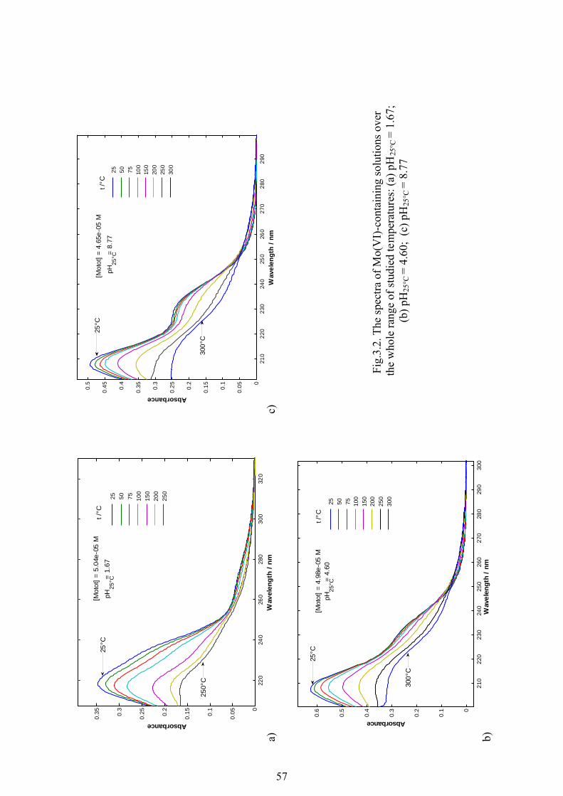
57
a)22
024
026
028
030
032
00
0.050.
1
0.150.
2
0.250.
3
0.35
Wav
elen
gth
/nm
Absorbance
25 50 75 100
150
200
250
pH=
1.67
25°C
[Mot
ot]=
5.04
e-05
Mt /
°C25
°C
250°
C
b)21
022
023
024
025
026
027
028
029
030
0
0
0.1
0.2
0.3
0.4
0.5
0.6
Wav
elen
gth
/nm
Absorbance
25 50 75 100
150
200
250
300
25°C
300°
C
t /°C
[Mot
ot]=
4.98
e-05
MpH
=4.
6025
°C
c)21
022
023
024
025
026
027
028
029
00
0.050.
1
0.150.
2
0.250.
3
0.350.
4
0.450.
5
Wav
elen
gth
/nm
Absorbance
25 50 75 100
150
200
250
300
[Mot
ot]=
4.65
e-05
M
pH=
8.77
25°C
t /°C
25°C
300°
C
Fig.
3.2.
The
spec
tra o
f Mo(
VI)
-con
tain
ing
solu
tions
ove
r th
e w
hole
rang
e of
stud
ied
tem
pera
ture
s: (a
) pH
25°C
= 1.
67;
(b) p
H25
°C=
4.60
; (c
) pH
25°C
= 8.
77

58
210
220
230
240
250
260
270
280
0
0.1
0.2
0.3
0.4
0.5
Wav
elng
th /
nm
Absorbance2.
212.
422.
943.
323.
814.
254.
644.
995.
305.
595.
745.
946.
306.
53
pH6.
53
2.94
2.21
50°C
[Mot
ot]=
5.2e
-05
M
200
210
220
230
240
250
260
270
280
0
0.050.
1
0.150.
2
0.250.
3
0.350.
4
0.450.
5
Absorbance
Wav
elen
gth
/nm
1.79
2.03
2.22
2.43
2.95
3.31
3.79
4.29
4.81
5.26
5.61
5.90
6.03
6.18
6.38
6.44
6.44
2.22
pH
100°
C
[Mot
ot]=
5.2e
-06
M
200
210
220
230
240
250
260
270
280
290
300
0
0.1
0.2
0.3
0.4
0.5
Absorbance
Wav
elen
gth
/nm
1.59
1.81
2.05
2.24
2.44
2.96
3.33
3.82
5.15
5.76
6.09
6.29
6.34
6.40
6.39
6.47
6.47
6.51
6.61
7.01
pH
150°
C
[Mot
ot]=
5.2e
-05
M
7.01
2.24
200
210
220
230
240
250
260
270
280
290
300
0
0.050.
1
0.150.
2
0.250.
3
0.350.
4
0.45
Absorbance
Wav
elen
gth
/nm
1.37
1.62
1.84
2.08
2.26
2.47
2.99
3.36
3.84
4.40
5.77
6.46
6.63
6.71
6.74
6.78
6.83
6.90
6.97
[Mot
ot]=
5.2e
-05
M
200°
CpH
6.97
2.26
Fig.
3.3
. Spe
ctra
ofm
olyb
denu
m (V
I) a
queo
usso
lutio
ns(c
orre
cted
forb
ackg
roun
dab
sorb
ance
) as a
func
tion
of p
H a
t diff
eren
tte
mpe
ratu
res.

59
210 220 230 240 250 260 270 280 290 3000
0.2
0.4
0.6
0.8
1
1.2
1.4
1.6
1.8
2
Abs
orba
nce
Wavelength / nm
3.173.654.244.525.125.225.716.366.716.756.776.796.816.836.906.957.107.277.688.17
250°C
[Motot] = 5.4e-05 M
pH
8.17
6.95
3.17
Fig. 3.4. Spectra of molybdenum (VI) aqueous solutions (not corrected for OH− and ClO4
− background absorbance ) as a function of pH at 250°C.
The fit for the case when the two absorbing species in solution are H2MoO4 and
MoO42- (model IIb, representing deprotonation in one step) is significantly worse, than for
the case when only HMoO4- and MoO4
2- are considered (model IIa), (fig.3.5c and 3.5c
respectively). Based on this together with the fact that the calculated values for log10K2 for
models I and IIa are in excellent agreement, the results for model IIb were discarded from
further consideration.
The values of ionisation constants for molybdic acid at different temperatures are given
in the table 3.2 and are plotted in fig. 3.6. The uncertainties in the pK’s were evaluated using
a Monte Carlo simulation (10000 iterations) of experimental errors arising from solution
preparation, temperature and absorbance. The influence of temperature uncertainty on the
density of water and ionisation constants of water as well as solution preparation were
similarly evaluated (separately) using the on a Monte Carlo method.

60
Fig.
3.5a
.Cal
cula
ted
(blu
e)an
dex
perim
enta
l (re
d) sp
ectra
and
thei
r res
idua
ls a
t diff
eren
ttem
pera
ture
s:m
odel
I (a
llth
ree
abso
rbin
gsp
ecie
sare
cons
ider
ed,i
.e.H
2MoO
4, H
MoO
4− and
MoO
42-).

61
210
220
230
240
250
260
270
280
0
0.1
0.2
0.3
0.4
0.5
spec
tra
210
220
230
240
250
260
270
280
-0.0
1
-0.0
050
0.00
5
0.01
resi
dual
s
Absorbance
Wav
eleng
th/n
m
150°
C
210
220
230
240
250
260
270
280
0
0.1
0.2
0.3
0.4
spec
tra
210
220
230
240
250
260
270
280
-0.0
1
-0.0
050
0.00
5
0.01
resi
dual
s
Absorbance
Wav
elen
gth
/nm
200°
C
220
230
240
250
260
270
0
0.1
0.2
0.3
0.4
spec
tra
210
220
230
240
250
260
270
280
-0.0
1
-0.0
050
0.00
5
0.01
resi
duals
Absorbance
Wav
elen
gth
/nm
250°
C
Fig.
3.5
b. C
alcu
late
d (b
lue)
and
expe
rimen
tal (
red)
spec
tra a
nd th
eir
resi
dual
sat
diff
eren
ttem
pera
ture
s:m
odel
IIa
(2ab
sorb
ing
spec
ies:
HM
oO4- an
dM
oO42-
).
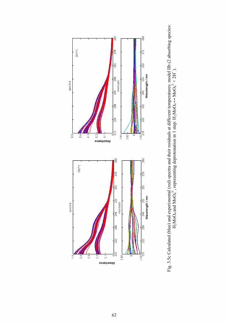
62
Fig.
3.5
c C
alcu
late
d (b
lue)
and
exp
erim
enta
l (re
d) sp
ectra
and
thei
r res
idua
ls a
t diff
eren
t tem
pera
ture
s:m
odel
IIb
(2 a
bsor
bing
spec
ies:
H2M
oO4
and
MoO
42-, r
epre
sent
ing
depr
oton
atio
n in
1 st
ep: H
2MoO
4↔
MoO
42-+
2H+
).
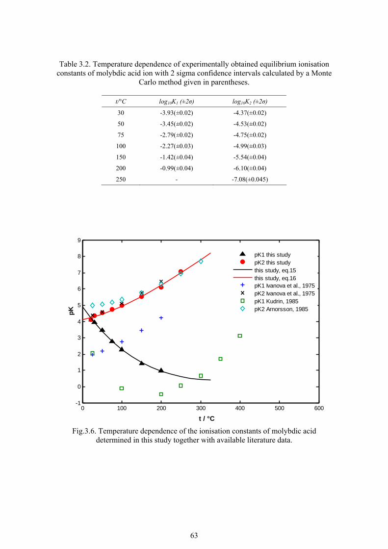
63
Table 3.2. Temperature dependence of experimentally obtained equilibrium ionisation constants of molybdic acid ion with 2 sigma confidence intervals calculated by a Monte
Carlo method given in parentheses.
t/°C log10K1 (±2σ) log10K2 (±2σ)
30 -3.93(±0.02) -4.37(±0.02)
50 -3.45(±0.02) -4.53(±0.02)
75 -2.79(±0.02) -4.75(±0.02)
100 -2.27(±0.03) -4.99(±0.03)
150 -1.42(±0.04) -5.54(±0.04)
200 -0.99(±0.04) -6.10(±0.04)
250 - -7.08(±0.045)
0 100 200 300 400 500 600-1
0
1
2
3
4
5
6
7
8
9
pK
t / °C
pK1 this studypK2 this studythis study, eq.15this study, eq.16pK1 Ivanova et al., 1975pK2 Ivanova et al., 1975pK1 Kudrin, 1985pK2 Arnorsson, 1985
Fig.3.6. Temperature dependence of the ionisation constants of molybdic acid
determined in this study together with available literature data.

64
The agreement between our data for the first ionisation constant and those reported
in the literature is poor, while values of the second ionisation constant appear to be more
consistent. The agreement between our values of pK2 and those, obtained by Ivanova et al.
(1975) is surprisingly good over the whole range of studied temperatures, given the
assumptions in their calculations. Two different reasons might account for the discrepancy
between the values for the pK1. Values of Kudrin (1985) were calculated from the Gibbs
energies, obtained from solubility measurements of tugarinovite in the range of 250-450°C,
and used for the extrapolation to lower temperatures. An inherent assumption in the
approach of Ivanova et al. (1975) was that the same value for the entropy change of the first
dissociation reaction for all weak acids (i.e. -79.496 J·mol-1·K-1) is applicable to molybdic
acid. However, any change of molybdenum coordination in the first ionisation step (eq. 3.1)
(see previous chapter) could result in significant errors in the estimates of the first ionisation
constant.
In fig.3.7 distribution diagrams of molybdic acid species at different temperatures
are shown. One can see that the fully protonated species loses its significance as the
temperature increases in studied pH interval. Thus, within the range of pH’s characteristic of
natural hydrothermal fluids in the Earth’s crust, HMoO4− and MoO4
2− species will
predominate. The molar absorptivities of the three molybdic acid species at 50°C and 150°C
are shown in fig. 3.8.
The deprotonation constants for molybdic acid were fitted as a function of
temperature with various extentions of the van’t Hoff equation, given by,
)ln(log 210 Te
TdTcTbaK ⋅++⋅+⋅+= (3.14)
The three term version of equation 3.14 gave the best fit for both constants with the
following coefficients:
)ln(660.1702875.0125.96log 110 TTK ⋅+⋅−−= (3.15)
)ln(9366.502690.0082.30log 210 TTK ⋅+⋅−−= (3.16)

65
2.5 3 3.5 4 4.5 5 5.5 6 6.5 70
10
20
30
40
50
60
70
80
90
100
pH
30 °C%
Mo to
t
HMoO4-
MoO42-
H2MoO40
2 3 4 5 6 7
10
20
30
40
50
60
70
80
90
100
pH
50 °C
%M
o tot
HMoO4-
MoO42-
H2MoO40
1 2 3 4 5 6 70
10
20
30
40
50
60
70
80
90
100
pH
75 °C
%M
o tot
HMoO4- MoO4
2-H2MoO40
2 3 4 5 6 70
10
20
30
40
50
60
70
80
90
100
pH
100 °C
%M
o tot
HMoO4- MoO4
2-H2MoO40
1 2 3 4 5 6 7 8 90
10
20
30
40
50
60
70
80
90
100
pH
150 °C
%M
o tot
HMoO4-
MoO42-
H2MoO40
1 2 3 4 5 6 7 80
10
20
30
40
50
60
70
80
90
100
pH
200 °C
%M
o tot
HMoO4- MoO4
2-
H2MoO40
4 4.5 5 5.5 6 6.5 7 7.5 8 8.5 90
10
20
30
40
50
60
70
80
90
100
pH
250 °C
%M
o tot
HMoO4-
MoO42-
Fig. 3.7. Distribution diagram of Mo (VI) aqueous species at studied temperatures.
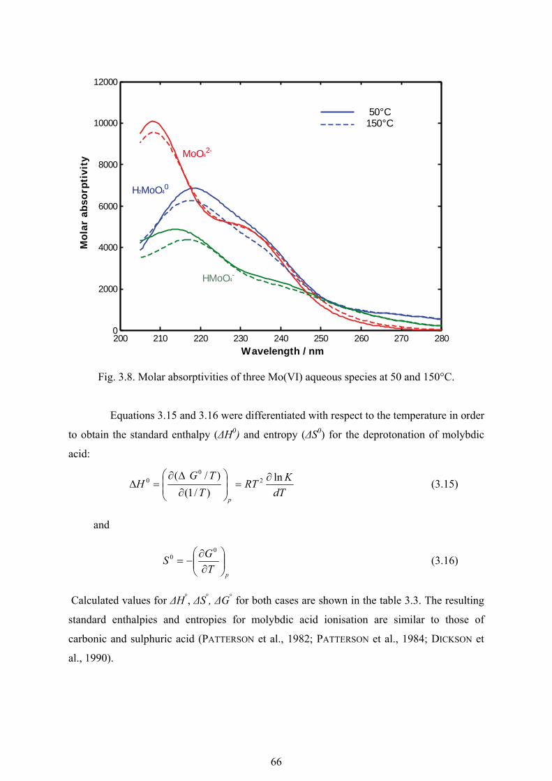
66
200 210 220 230 240 250 260 270 2800
2000
4000
6000
8000
10000
12000M
olar
abso
rpti
vity
Wavelength / nm
50°C150°C
HMoO4-
H2MoO40
MoO42-
Fig. 3.8. Molar absorptivities of three Mo(VI) aqueous species at 50 and 150°C.
Equations 3.15 and 3.16 were differentiated with respect to the temperature in order
to obtain the standard enthalpy (ΔH0) and entropy (ΔS0) for the deprotonation of molybdic
acid:
dTKRT
TTG
Hp
ln)/1(
)/( 20
0 ∂=⎟
⎟⎠
⎞⎜⎜⎝
⎛
∂
Δ∂=Δ (3.15)
and
pTGS ⎟⎟
⎠
⎞⎜⎜⎝
⎛∂∂
−=0
0 (3.16)
Calculated values for ΔH°, ΔS°, ΔG° for both cases are shown in the table 3.3. The resulting
standard enthalpies and entropies for molybdic acid ionisation are similar to those of
carbonic and sulphuric acid (PATTERSON et al., 1982; PATTERSON et al., 1984; DICKSON et
al., 1990).

67
Table 3.3. Temperature dependence of thermodynamic values for the ionisation reactions of molybdic acid (eq.3.1 and 3.2).
t / °C
ΔG01
kJ·mol-1
ΔG0
2 kJ·mol-1
ΔH0
1 kJ·mol-1
ΔH0
2 kJ·mol-1
ΔS0
1 J·K-1·mol-1
ΔS0
2 J·K-1·mol-1
25 23.26 24.40 51.85 -11.88 95.89 -121.67
30 22.78 25.01 51.89 -12.86 96.01 -124.92
50 20.86 27.64 51.75 -17.03 95.60 -138.25
75 18.50 31.32 50.97 -22.83 93.27 -155.52
100 16.21 35.43 49.50 -29.27 89.20 -173.37
150 12.04 45.02 44.49 -44.08 76.68 -210.55
200 8.62 56.51 36.73 -61.46 59.41 -249.33
250 6.16 69.97 26.23 -81.42 38.35 -289.38
300 4.84 85.46 12.97 -103.95 14.18 -330.47

68
3.5. References
Arnorsson S. and Ivarsson G. (1985) Molybdenum in Icelandic geothermal waters.
Contributions to Mineralogy and Petrology 90(2-3), 179-89. Boily J.-F. and Suleimenov O. M. (2006) Extraction of Chemical Speciation and Molar
Absorption Coefficients with Well-Posed Solutions of Beer's Law. Journal of Solution Chemistry 35(6), 917-926.
Dickson A. G., Wesolowski D. J., Palmer D. A., and Mesmer R. E. (1990) Dissociation constant of bisulfate ion in aqueous sodium chloride solutions to 250°C. Journal of Physical Chemistry 94(12), 7978-7985.
Fernandez D. P., Goodwin A. R. H., Lemmon E. W., Sengers J. M. H. L., and Williams R. C. (1997) A formulation for the static permittivity of water and steam at temperatures from 238 K to 873 K at pressures up to 1200 MPa, including derivatives and Debye-Hueckel coefficients. Journal of Physical and Chemical Reference Data 26(4), 1125-1166.
Graham R. L. and Hepler L. G. (1956) Heats of formation of sodium molybdate, molybdic acid, and aqueous molybdate ion. Journal of the American Chemical Society 78, 4846-8.
Ho P. C. and Palmer D. A. (1996) Ion association of dilute aqueous sodium hydroxide solutions to 600 DegC and 300 MPa by conductance measurements. Journal of Solution Chemistry 25(8), 711-729.
Ivanova G. F., Levkina N. I., Nesterova L. A., Zhidikova A. P., and Khodakovskii I. L. (1975) Equilibria in the molybdenum trioxide-water system in the 25-300°C range. Geokhimiya 2, 234-247.
Kudrin A. V. (1985) Experimental study of solubility of tugarinovite MoO2 in aqueous solutions at high temperatures. . Geokhimiya 6, 870-83.
Maksimova I. N., Pravdin N. N., and Razuvaev V. E. (1976) Study of hydrolysis of sodium chromate, molybdate, and tungstate in aqueous solutions at 15-90 Deg. Ukrainskii Khimicheskii Zhurnal (Russian Edition) 42(10), 1019-23.
Marshall W. L. and Franck E. U. (1981) Ion product of water substance, 0-1000°C, 1-10,000 bars, new international formulation and its background. Journal of Physical and Chemical Reference Data 10(2), 295-304.
Patterson C. S., Slocum G. H., Busey R. H., and Mesmer R. E. (1982) Carbonate equilibriums in hydrothermal systems: first ionization of carbonic acid in sodium chloride media to 300°C. Geochimica et Cosmochimica Acta 46(9), 1653-63.
Patterson C. S., Busey R. H., and Mesmer R. E. (1984) Second ionisation of carbonic acid in sodium chloride media to 250°C. Journal of Solution Chemistry 13(9), 647-661.
Ratcliffe C. I. and Irish D. E. (1984) Vibrational spectral studies of solutions at elevated temperatures and pressures. VI. Raman studies of perchloric acid. Canadian Journal of Chemistry 62(6), 1134-44.
Solymosi F. (1977) Thermal stability of perchloric acid. Acta Physica et Chemica 23(2-3), 317-54.
Suleimenov O. M. and Seward T. M. (2000) Spectrophotometric measurements of metal complex formation at high temperatures: the stability of Mn(II) chloride species. Chemical Geology 167(1-2), 177-192.
Swaddle T. W., Henderson M. P., and Miasek V. I. (1971) Kinetics of thermal decomposition of aqueous perchloric acid. Canadian Journal of Chemistry 49(2), 317-24.

69
Urusov V. S., Ivanova G. F., and Khodakovskii I. L. (1967) Energy and thermodynamic characteristics of tungstates and molybdates in connection with some features of their geochemistry. Geokhimiya(10), 1050-63.
Wagner W. (1998) Properties of Water and Steam/The Industrial Standard IAPWS-IF97 for the Thermodynamic Properties and Supplementary Equations for Other Properties.
Zhidikova A. P. and Khodakovskii I. L. (1971) Powellite activity product at 25°C. Geokhimiya 4, 427-432.
Zhidikova A. P. and Kuskov O. L. (1971) Determination of thermodynamic constants of calcium molybdate (powellite) and sodium molybdate. Geokhimiya 9, 1149-1151.
Zhidikova A. P., Khodakovskii I. L., Urusova M. A., and Valyashko V. M. (1973) Experimental determination of the activity coefficients of sodium molybdate in aqueous solutions at 25 and 300°C. Zhurnal Neorganicheskoi Khimii 18(5), 1160-1165.
Zinov'ev A. A. and Babaeva V. P. (1961) The thermal decomposition of perchloric acid. Zhurnal Neorganicheskoi Khimii 6, 271-82.

70
3.6. Appendix
Appendix 3.6.1. Initial composition of the Mo(VI)-containing experimental solutions used for obtaining ionisation constants at 30-200°C.
Motot Natot ClO4 tot pH25°C
1 4.84E-05 9.68E-05 4.98E-02 1.31
2 4.79E-05 9.58E-05 2.81E-02 1.55
3 4.92E-05 9.84E-05 1.69E-02 1.77
4 4.34E-05 8.69E-05 9.78E-03 2.01
5 4.32E-05 8.64E-05 6.37E-03 2.20
6 4.83E-05 9.66E-05 3.97E-03 2.41
7 5.55E-05 1.11E-04 1.25E-03 2.94
8 5.07E-05 1.01E-04 5.59E-04 3.33
9 5.48E-05 1.10E-04 2.21E-04 3.84
10 5.14E-05 1.03E-04 9.70E-05 4.25
11 5.36E-05 1.07E-04 4.85E-05 4.57
12 5.33E-05 1.07E-04 2.46E-05 4.86
13 5.19E-05 1.04E-04 1.26E-05 5.15
14 5.31E-05 1.06E-04 6.71E-06 5.42
15 5.10E-05 1.02E-04 4.67E-06 5.57
16 5.13E-05 2.03E-04 1.04E-04 5.78
17 4.93E-05 9.85E-05 2.93E-06 5.76
18 5.25E-05 1.05E-04 1.26E-06 6.14
19 5.18E-05 1.91E-04 8.81E-05 6.38
20 4.88E-05 9.77E-05 5.92E-07 6.44
21 5.37E-05 2.06E-04 9.87E-05 7.36
22 5.61E-05 2.09E-04 9.64E-05 7.54
23 5.62E-05 2.07E-04 9.14E-05 8.47
24 5.68E-05 1.24E-04 0 8.99
25 5.61E-05 2.84E-04 1.52E-04 9.27
26 6.32E-05 1.66E-04 0 9.58
27 5.70E-05 1.95E-04 0 9.89
28 5.51E-05 3.70E-04 0 10.39
29 5.56E-05 9.74E-04 0 10.90

71
Appendix 3.6.2. Initial composition of the Mo(VI)-containing experimental solutions used for obtaining ionisation constants at 250°C.
Motot Natot ClO4 tot pH25°C
1 4.84E-05 9.68E-05 9.01E-04 3.05
2 5.10E-05 1.02E-04 3.30E-04 3.48
3 5.12E-05 1.02E-04 1.23E-04 3.91
4 5.65E-05 1.13E-04 6.47E-05 4.19
5 5.10E-05 1.02E-04 4.84E-05 4.32
6 5.01E-05 1.00E-04 2.94E-05 4.53
7 5.13E-05 2.03E-04 1.04E-04 5.78
8 5.18E-05 1.91E-04 8.81E-05 6.38
9 5.37E-05 2.06E-04 9.87E-05 7.36
10 5.61E-05 2.09E-04 9.64E-05 7.54
11 5.62E-05 2.07E-04 9.14E-05 8.47
12 5.68E-05 1.24E-04 0 8.99
13 5.61E-05 2.84E-04 1.52E-04 9.27
14 6.32E-05 1.66E-04 0 9.58
15 5.70E-05 1.95E-04 0 9.89
16 5.51E-05 3.70E-04 0 10.39
17 5.56E-05 9.74E-04 0 10.90

72
4. Tungstic acid ionisation at 25-300°C
4.1. Introduction Unlike the Mo (VI) system, the simple mononuclear tungstate equilibra have been
less thoroughly studied at ambient temperatures although a few more experimental studies
have been carried out at elevated temperatures. A number of previous studies have been
carried out on the tungstate polyanions by Jander (1929) (spectrophotometry), Spytsyn
(1960) (spectrophotometry + dilatometry), Sasaki (1961) (potentiometry) and Aveston
(1964) (raman spectroscopy + ultracentrifugation). The first studies which reported values of
the equilibrium constants for the ionisation equilibria of tungstic acid were those of
Schwarzenbach (1958), who carried out potentiometric measurements in a streaming
apparatus at 20°C and those of Yatsimirsky (1964; 1965), who studied the kinetics of the
catalytic oxidation of iodide ion with hydrogen peroxide in the presence of W(VI) at 25°C.
Afterwards Ivanova (1968), derived an equation of temperature dependence for both
dissociation constants of tungstic acid up to 350°C which was based on the assumption that
ΔSdiss for the most of the acids have similar values (average of -79.496 J·mol-1·K-1 and -
125.52 J·mol-1·K-1 for the first and second dissociation step respectively). Bryzgalin (1983)
employed an empirical electrostatic model to calculate the ionisation constants in 25-300°C
range. In addition, the solubilities of scheelite, tungsten(VI) oxide and tungstic acid have
been measured at elevated temperatures by several authors (YASTREBOVA et al., 1963;
BRYZGALIN, 1976; FOSTER, 1977; WOOD and VLASSOPOULOS, 1989; WOOD, 1992). The
relationships between monomeric and polynulcear forms of W(VI) in 100-300°C range have
been studied by potentiometric titrations of Na-WO4-Cl-H2O solutions by Wesolowski
(1984) . The complexity of the W(VI) system is mainly due to the presence of polynuclear
species which occur in quite dilute solutions with ΣW≥ 10-5 mol·dm-3 .
The aim of this study was therefore to determine the ionisation constants of
monomeric tungstic acid in 25-300°C temperature range by spectrophotometric methods in
dilute solutions in order to avoid influence of polynuclear apecies.
4.2. Experimental method The solutions were prepared on a molal scale with Nanopure Millipore water
(resistivity >18MΩ/cm). Perchloric acid stock solution was diluted from concentrated acid
(HClO4, 60%, p.a., Merck) and standardized by colorimetric titration against dried Trisma-
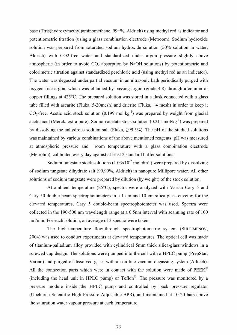
73
base (Ttris(hydroxymethyl)aminomethane, 99+%, Aldrich) using methyl red as indicator and
potentiometric titration (using a glass combination electrode (Metroom). Sodium hydroxide
solution was prepared from saturated sodium hydroxide solution (50% solution in water,
Aldrich) with CO2-free water and standardized under argon pressure slightly above
atmospheric (in order to avoid CO2 absorption by NaOH solutions) by potentiometric and
colorimetric titration against standardized perchloric acid (using methyl red as an indicator).
The water was degassed under partial vacuum in an ultrasonic bath periodically purged with
oxygen free argon, which was obtained by passing argon (grade 4.8) through a column of
copper fillings at 425°C. The prepared solution was stored in a flask connected with a glass
tube filled with ascarite (Fluka, 5-20mesh) and drierite (Fluka, +4 mesh) in order to keep it
CO2-free. Acetic acid stock solution (0.199 mol·kg-1) was prepared by weight from glacial
acetic acid (Merck, extra pure). Sodium acetate stock solution (0.211 mol·kg-1) was prepared
by dissolving the anhydrous sodium salt (Fluka, ≥99.5%). The pH of the studied solutions
was maintained by various combinations of the above mentioned reagents. pH was measured
at atmospheric pressure and room temperature with a glass combination electrode
(Metrohm), calibrated every day against at least 2 standard buffer solutions.
Sodium tungstate stock solutions (1.03x10⁻² mol·dm-3) were prepared by dissolving
of sodium tungstate dihydrate salt (99,99%, Aldrich) in nanopure Millipore water. All other
solutions of sodium tungstate were prepared by dilution (by weight) of the stock solution.
At ambient temperature (25°C), spectra were analyzed with Varian Cary 5 and
Cary 50 double beam spectrophotometers in a 1 cm and 10 cm silica glass cuvette; for the
elevated temperatures, Cary 5 double-beam spectrophotometer was used. Spectra were
collected in the 190-500 nm wavelength range at a 0.5nm interval with scanning rate of 100
nm/min. For each solution, an average of 3 spectra were taken.
The high-temperature flow-through spectrophotometric system (SULEIMENOV,
2004) was used to conduct experiments at elevated temperatures. The optical cell was made
of titanium-palladium alloy provided with cylindrical 5mm thick silica-glass windows in a
screwed cup design. The solutions were pumped into the cell with a HPLC pump (PrepStar,
Varian) and purged of dissolved gases with an on-line vacuum degassing system (Alltech).
All the connection parts which were in contact with the solution were made of PEEK®
(including the head unit in HPLC pump) or Teflon®. The pressure was monitored by a
pressure module inside the HPLC pump and controlled by back pressure regulator
(Upchurch Scientific High Pressure Adjustable BPR), and maintained at 10-20 bars above
the saturation water vapour pressure at each temperature.

74
Spectra of blank solutions for all studied temperatures were taken before and after
each solution. Three consecutive spectra were taken for each solution at each temperature.
Spectra were measured 15-20 minutes after the desired temperature was reached to allow the
temperature equilibration. The total concentration of tungsten was low and ranged from
0.114 to 0.002 mmol·kg-1 (Appendix 4.4.1). All spectra were corrected for background
absorbance (windows+water+ClO4−,OH−, CH3COO− or CH3COOH). Molar absorptivities of
ClO4−, OH−, CH3COO− or CH3COOH were obtained from the spectra of the pure solutions
which were measured separately at each studied temperature.
4.3. Results and discussion The mathematical analysis and spectrophotometric data processing were exactly the
same as described for Mo(VI) system in the earlier chapters.
4.3.1. Experiments at ambient temperature.
The spectra of tungsten (VI)-containing aqueous solutions with a total maximum W
concentration of~1x10⁻⁴ mol·dm-3 and different values of pH are shown in fig.4.1. Note,
that the normalised absorbance refers to the measured absorbance divided (i.e. normalised)
by the total tungsten concentration for the purpose of comparison.
In addition, two tungsten(VI)-containing solutions of similar total concentration of
W and pH (i.e. 1.064x10⁻⁴ mol·dm-3 , pH=3.66 and 1.071x10⁻⁴ mol·dm-3, pH=3.68), one of
which was adjusted just with acetic acid, and the other buffered with the acetate buffer were
analyzed separately over period of two 2 weeks with spectra recorded every 2 hours. The
results are shown in fig.4.2. Such changes in spectra of the same solution can be an evidence
of slowly forming polynuclear species. One can see that the spectra are still changing after
400 hours in both cases although buffering seems to dampen the changes arising form the
formation and disproportionation of polymeric species.
Several sets of solutions with the lower total concentrations of W (i.e. 5.0x10⁻⁵
mol·dm-3, 8.5x10⁻⁶ mol·dm-3 and 2.7x10⁻⁶ mol·dm-3) and different pH’s were studied. For the
case of 8.5x10⁻⁶ mol·dm-3 and 2.7x10⁻⁶ mol·dm-3 total tungsten concentrations, a 10 cm
quartz cuvette was used .The results are shown in fig.4.3. The changes in the spectra caused
by dilution of the solution can be clearly seen (compare fig.4.1). In addition to the expected
decrease in absorbances values due to dilution, there is also an overall smoothing of the
absorbance curve with the absence of various shoulders attributed to polymeric species.
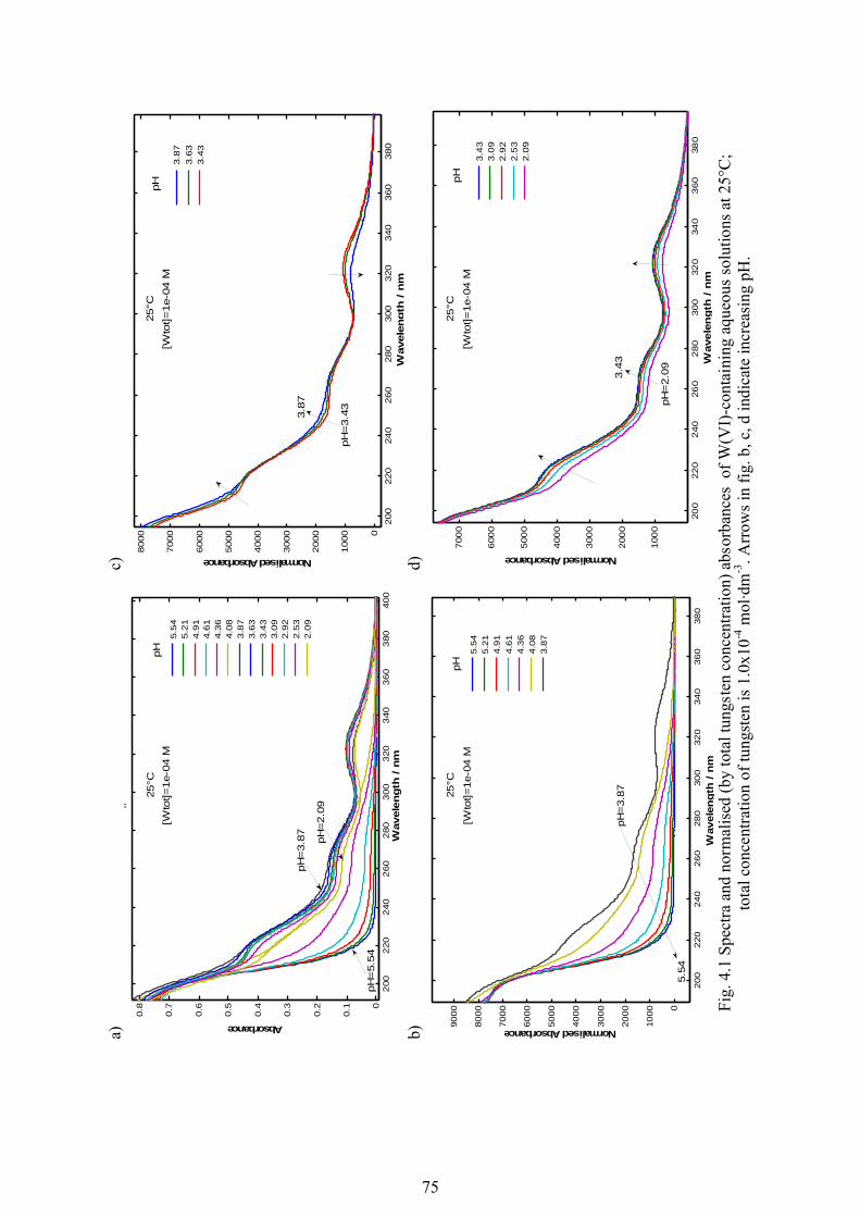
75
a)
200
220
240
260
280
300
320
340
360
380
400
0
0.1
0.2
0.3
0.4
0.5
0.6
0.7
0.8
Wav
elen
gth
/nm
Absorbance
n
5.54
5.21
4.91
4.61
4.36
4.08
3.87
3.63
3.43
3.09
2.92
2.53
2.09
pH=
3.87 pH
=2.
09
pH=
5.54
pH[W
tot]=
1e-0
4M
25°C
b)
200
220
240
260
280
300
320
340
360
380
0
1000
2000
3000
4000
5000
6000
7000
8000
9000
NormalisedAbsorbance
Wav
elen
gth
/nm
5.54
5.21
4.91
4.61
4.36
4.08
3.87
pH
pH=
3.87
5.54
25°C
[Wto
t]=1e
-04
M
c)
200
220
240
260
280
300
320
340
360
380
0
1000
2000
3000
4000
5000
6000
7000
8000
NormalisedAbsorbance
Wav
elen
gth
/n
m
3.8
73.6
33.
43
pH
pH=
3.433.
87
25°C
[Wto
t]=1e
-04
M
d)
200
220
240
260
280
300
320
340
360
380
100
0
200
0
300
0
400
0
500
0
600
0
700
0
NormalisedAbsorbance
Wav
elen
gth
/n
m
3.4
33.
09
2.9
22.
53
2.09
pH
pH=
2.093.43
[Wto
t]=1e
-04
M
25°C
Fig.
4.1
Spe
ctra
and
nor
mal
ised
(by
tota
l tun
gste
n co
ncen
tratio
n) a
bsor
banc
es o
fW(V
I)-c
onta
inin
gaq
ueou
ssol
utio
nsat
25°C
;to
talc
once
ntra
tion
of tu
ngst
en is
1.0
x10-4
mol
·dm
-3. A
rrow
s in
fig. b
, c, d
indi
cate
incr
easi
ng p
H.
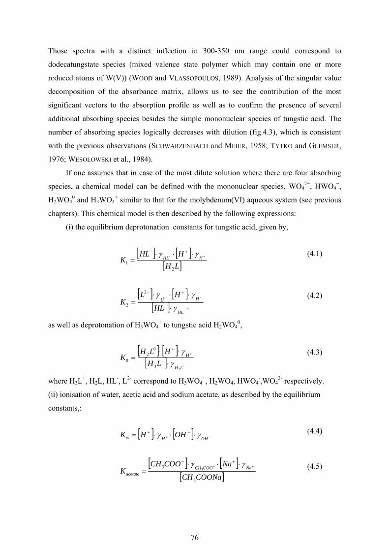
76
Those spectra with a distinct inflection in 300-350 nm range could correspond to
dodecatungstate species (mixed valence state polymer which may contain one or more
reduced atoms of W(V)) (WOOD and VLASSOPOULOS, 1989). Analysis of the singular value
decomposition of the absorbance matrix, allows us to see the contribution of the most
significant vectors to the absorption profile as well as to confirm the presence of several
additional absorbing species besides the simple mononuclear species of tungstic acid. The
number of absorbing species logically decreases with dilution (fig.4.3), which is consistent
with the previous observations (SCHWARZENBACH and MEIER, 1958; TYTKO and GLEMSER,
1976; WESOLOWSKI et al., 1984).
If one assumes that in case of the most dilute solution where there are four absorbing
species, a chemical model can be defined with the mononuclear species, WO42−, HWO4
−,
H2WO40 and H3WO4
+ similar to that for the molybdenum(VI) aqueous system (see previous
chapters). This chemical model is then described by the following expressions:
(i) the equilibrium deprotonation constants for tungstic acid, given by,
[ ] [ ][ ]LH
HHLK HHL
21
+− ⋅⋅⋅=
+− γγ (4.1)
[ ] [ ][ ] ⋅⋅
⋅⋅⋅=
−
+−
−
+−
HL
HL
HL
HLK
γ
γγ2
2
2
(4.2)
as well as deprotonation of H3WO4+ to tungstic acid H2WO4
0,
[ ] [ ][ ] +
+
⋅
⋅⋅= +
+
LH
H
LHHLH
K3
3
02
0 γγ (4.3)
where H3L+, H2L, HL-, L2- correspond to H3WO4+, H2WO4, HWO4
-,WO42- respectively.
(ii) ionisation of water, acetic acid and sodium acetate, as described by the equilibrium
constants,:
[ ] [ ] −+ ⋅⋅⋅= −+OHHw OHHK γγ (4.4)
[ ] [ ][ ]COONaCH
NaCOOCHK NaCOOCH
acetate3
33
+− ⋅⋅⋅=
+− γγ (4.5)

77
a)
200
220
240
260
280
300
320
340
360
0.1
0.2
0.3
0.4
0.5
0.6
0.7
0.8
0.91
1.1
Wav
ele
ng
th /
nm
Absorbance
25
°C
[Wto
t]=
1e
-04
M
pH
=3
.66
(unbu
ffe
red
)
010
020
030
040
00.
1
0.12
0.14
0.16
0.18
time/
hour
s
Abs
320n
m
010
020
030
040
00.
2
0.250.3
0.350.4
time/
hour
s
260n
m
010
020
030
040
00.
5
0.550.6
0.650.7
time/
hour
s
Abs
220n
m
010
020
030
040
00.
250.3
0.350.4
0.45
time/
hour
s
240n
m
b)
200
220
240
260
280
300
320
340
360
380
0
0.2
0.4
0.6
0.81
1.2
Wa
vele
ng
th/
nm
Absorbance
25
°C
[
Wto
t]=
1e
-04
Mp
H=
3.6
8(b
uff
ere
d)
010
020
030
040
00.
02
0.04
0.06
0.080.1
time/
hour
s
Abs
320n
m
010
020
030
040
0
0.2
0.250.3
time/
hour
s
260n
m
010
020
030
040
0
0.56
50.
570.
575
0.58
0.58
50.
59
time/
hour
sAbs
220n
m
010
020
030
040
00.
27
0.28
0.290.3
0.31
0.32
time/
hour
s
240n
m
Fig.
4.2.
Spe
ctra
ofW
(VI)
-con
tain
ing
solu
tion
at fi
xed
pH, t
aken
dur
ing
16 d
ays a
nd th
e ch
ange
sof
abso
rban
cesw
ithth
etim
e a
t cho
sen
wav
elen
gth.
a)pH
=3.6
8, n
o bu
ffer
;b) p
H=3
.66,
adj
uste
d w
ith a
ceta
te b
uffe
r.
490n
m
490n
m

78
a)
200 220 240 260 280 300 320 340
0
0.05
0.1
0.15
0.2
0.25
0.3
0.35
0.4
Wavelength / nm
Abs
orba
nce
5.214.924.624.344.113.873.603.433.082.922.552.101.571.23
[Wtot]=5e-05 M25°C pH
pH=5.21
pH=3.60
pH=2.10
200 220 240 260 280 300 320 340
-0.14
-0.12
-0.1
-0.08
-0.06
-0.04
-0.02
0
0.02
0.04
Wavelength / nm
UxS
25°C[Wtot]=5e-05 M
4
2
5
3
1
6
b)
200 220 240 260 280 300 320 340 360
0
0.01
0.02
0.03
0.04
0.05
0.06
Wavelength / nm
Abs
orba
nce
1.121.371.652.002.272.612.903.203.503.804.064.384.684.975.24
pH25°C
[Wtot]=8.5e-06 M
pH=5.24
pH=2.90
pH=4.06
200 220 240 260 280 300 320 340 360-0.15
-0.1
-0.05
0
0.05
0.1
0.15
Wavelength / nm
UxS
n
25°C
[Wtot]=8.5e-06 M
3
4
1
2
5
c)
200 250 300 350
0
0.005
0.01
0.015
0.02
Wavelength / nm
Abs
orba
nce
5.285.094.864.664.474.294.063.853.663.453.253.062.782.472.161.861.57
pH=5.28
pH=1.57
pH=3.85
25°C
[Wtot]=2.8e-06 M
pH
200 220 240 260 280 300 320 340
-0.04
-0.02
0
0.02
0.04
0.06
Wavelength / nm
UxS
1
2
3
4
25°C
[Wtot]=2.7e-06 M
Fig.4.3. Spectra of W(VI) solutions with different values of pH and the contribution of most
significant vectors in total absorbance: a) [Wtot] = 5x10⁻⁵ mol·dm-3, b) [Wtot] = 8.5x10⁻⁶ mol·dm-3, c) [Wtot] = 2.8x10⁻⁶ mol·dm-3.

79
[ ] [ ][ ]COOHCH
HCOOCHK HCOOCH
acetic3
33
+− ⋅⋅⋅=
+− γγ (4.6)
(iii) charge balance equations:
[ ] [ ] [ ] [ ] [ ] [ ] [ ]++−−−−− +=++++ NaHCOOCHClOOHLHL 3422
(4.7)
(iv) mass balance equations for total molybdenum, total Na and total acetate:
[ ] [ ] [ ] [ ]−− ++= 22 LHLLHLtot
(4.8)
[ ] [ ] [ ]COONaCHNaNatot 3+= + (4.9)
[ ] [ ] [ ] [ ]−++= COOCHCOOHCHCOONaCHCOOCH tot 3333 (4.10)
The terms in square brackets are molal concentrations and γ is the molal activity coefficient
of the corresponding species and is taken as unity for uncharged species. Molar
concentrations of absorbing species used in Beer’s law in the cases when ionic strength was
not adjusted were calculated using the density of water taken from (WAGNER, 1998) (given
the low concentration of solution components). The values for pK for acetic acid and sodium
acetate at the saturated vapour pressure were taken from Mesmer et al. (1989) and Shock and
Koretsky (1993), respectively.
Activity coefficients for charged species were calculated using an extended Debye-
Hückel equation of the form:
IBaIAz
i
ii 0
2
10 1log
+−=γ (4.11)
where the Debye-Hückel limiting slope parameters A, B where taken from Fernandez et al.
(1997). The iterative calculation procedure was based on successive substitution with the
initial assumption that all the activity coefficients were equal to unity.
Applying the same calculation procedure as described in previous chapters, the
resulting values are as follows: pK1 = 4.24±0.08 , pK2 = 3.48±0.05, pK0= -0.35±0.75. The
error in pK0 is unacceptably high though the overall reproducibility of experimental
absorbance is satisfactory (see fig. 4.4). The values in pK1 and pK2 are close to those
reported by Schwarzenbach (1958) (see table 4.1). The other available experimental values

80
at ambient temperature have some consistency in pK2 values, but considerably differ with
respect to pK1. An attempt to calculate pK1 and pK2 by considering only the solutions with
pH>2.5 (therefore assuming the existence only of the three species, i.e. H2WO4, HWO4-,
WO42-, by analogy with the molybdate system) did not result in good fit. One reason for this
could be that there are only two significant vectors contributing in the total absorbance fig.
4.5). The other two vectors, which also contribute to the total absorbance at pH<2.5
(fig.4.3c) may arise from the commencement of polymerisation processes at low pH. It is
therefore probable that the good agreement with the data reported by Schwarzenbach et al.
(1958) are fortuitous and the equilibrium in the W(VI) solutions even at such low
concentrations may also involve the formation of polyanions. This conclusion is supported
by the fact that calculated molar absorptivity for the HWO4-species (fig.4.6) has bands in the
visible region, which are usually attributed to polyanions as discussed above.
Table 4.1. Previously reported values for W (VI) mononuclear equilibrium in the aqueous solution at ambient temperature. pK1 and pK2 are the first and second deprotonation
constants of tungstic acid.
t/
° C
Ionic
strength Medium pK1 pK2 pK0 Method Reference
25° 0 - 4.24 3.48 0.35 potentiometric
measurements This study
20 0.1 NaClO4 ≈4.6 ≈3.5 - potentiometric
measurements
Schwarzenbach et al.,
1962
22 - - 2.3 3.51 - kinetic of catalytic
oyxydation
Yatsimirski and Prik ,
1964
25 0.003 - 2.2 3.7 - kinetic of catalytic
oyxydation
Yatsimirski and
Romanov, 1965
25 0 - - 3.62 - potentiometric
measurements Wesolowski et al., 1984
25 - - 2.19 3.71 - thermodynamic
calculations
Ivanova and
Khodakovskii, 1968
25 - - 2.13 3.74 -
calculations based
on electrostatic
theory
Bryzgalin., 1983

81
200 250 300 350
0
0.005
0.01
0.015
0.02
200 250 300 350
-0.001-0.0005
00.00050.001
residuals
Wavelength / nm
Abso
rban
ce
spectra
Fig.4.4 Calculated (blue) and experimental (red) absorbances and their residuals for the
most diluted solutions ( [Wtot] = 2.8x10⁻⁶ mol·dm-3).
200 210 220 230 240 250 260-0.7
-0.6
-0.5
-0.4
-0.3
-0.2
-0.1
0
0.1
0.2
Wavelength / nm
UxS
1
2
Fig.4.5 The contribution of most significant vectors in total absorbance for the case
when [Wtot] = 2.8x10⁻⁶ mol·dm-3 and minimal value of solution’s pH is 2.5.

82
220 240 260 280 300 320 340
0
1
2
3
4
5
6
7
8
9
x 104
Wavelength / nm
Mol
arab
sorp
tivi
ty25°C
Fig.4.6. Molar apsorptivity for the W(VI) aqueous species at 25°C.
4.3.2. Experiments at elevated temperatures.
Unfortunately, our experimental set up did not allow us to use a high temperature cell
with the 10 cm path length therefore we were limited to work with the quite concentrated
solutions ([Wtot] = 7x10⁻⁵ - 1x10⁻⁴ mol·dm-3 , see Appendix 4.4.2) due to low absorbance of
the tungstate.
Increasing temperature should result in the decomposition of polytungstate species as
noted previously by Wesolowski (1990), which could be clearly seen in fig.4.7. Increasing
the temperature from 100 to 200°C (fig.4.7a) causes similar changes in the shape of the
spectra as dilution of the solution (described above as smoothing the shape of the spectra and
causing disappearance of bands in the visible region). The change of absorbance (at one
wavelength) versus time shows clearly that at 100 and 150°C, the changes in absorbance are
quite significant, while at 200 and 250°C the changes observed are very small and the
systems are more stable (fig. 4.7b and 4.7c). At 300°C the steady but small growth of
absorbance at every wavelength arises from light scattering due to progressive dissolution of
silica glass windows (as described in previous chapter) and is not due to the changes in
speciation in the solution.

83
Based on these observations, we decided to limit our high temperature study to two
temperatures 200 and 250 °C. Fig. 4.8 shows the spectra of W(VI)-containing solutions and
the contribution of the most significant vectors to the total absorbance at these temperatures.
In fig.4.9, the contribution of most significant vectors to the total absorbance is shown. As in
the case of Mo(VI) system, there are only two absorbing species at this temperatures in
studied pH interval. The calclulated values of pK2 for the reaction
+− +↔ HWOHWO 24
-4 (4.12)
are equal 6.31±0.1 and 6.79±0.11 at 200 and 250°C respectively. The reproducibility of
experimental absorbance by calculated absorbance and their residuals are shown in fig.10.
Calculated molar absorptivities at both temperatures are shown in fig.4.11.
Quite a considerable discrepancy between literature data (table 4.2) and data obtained
in this study may be explained by several reasons. Firstly, the data of Ivanova (1968) ,
Bryzgalin (1983) and Wood (2000) were not obtained experimentally. Secondly, the
presence of polynuclear species in the potentiometric study of Wesolowsky (WESOLOWSKI et
al., 1984) will affect the overall evaluation of the equilibrium constants (i.e. many adjustable
parameters in their chemical model). And finally, the fact that the maximum of the
absorbance for both of the studied W(VI) species is in vacuum ultraviolet region and we
were forced to work only with the low energy absorption edge of the spectra. Moreover, all
the components used for adjusting pH (acetic acid, sodium acetate and sodium hydroxide)
also absorb in this region and therefore, the small imprecisions in background absorbance
subtraction could give rise to inaccuracies in the resulting pK. Therefore, the agreement
between our values of pK2 and those of Ivanova and Khodakovsky (1968) perhaps
coincidental, given the complexity of the system and the assumptions involved in their
calculations.

84
Table 4.2. Previously reported values for mononuclear tungstate equilibria in the aqueous solution at elevated temperatures together with the values obtained in this study.
pK1 and pK2 are the first and second deprotonation constants of tungstic acid.
t/°C 50 100 150 200 250 300 Method Reference
pK2
-
-
-
6.31
6.79
-
uv-vis spectroscopy
this study
pK2 3.75 4.17 4.71 5.34 6.07 6.89
potentiometric
measurements
Wesolowski et al.,
1984
pK1 2.38 2.93 3.62 4.41 5.28 6.19
thermodynamic
calculations
Ivanova and
Khodakovskii, 1968
pK2
3.96
4.57
5.27
6.04
6.85
7.69
pK1 2.17 2.33 2.53 2.77 3.04 3.32
calculations based on
electrostatic theory
Bryzgalin., 1983
pK2
3.65
3.85
4.14
4.51
4.93
5.38
pK1 - - - 3.56 - 3.39
Calculations based on
HKF model1
Wood and Samson,
2000
pK2
-
-
-
5.15
-
6.48
1-pK values correspond to 500 kbar.

85
220
240
260
280
300
320
340
360
380
400
0
0.1
0.2
0.3
0.4
0.5
0.6
0.7
Wav
elen
gth
/nm
Absorbance
100
150
200
t/°C
[Wto
t]=9.
4e-0
5M
pH=3
.67
020
040
060
00.
04
0.06
0.080.1
0.12
time/
min
Abs
100°
C32
0nm
020
040
060
00.
18
0.18
5
0.19
0.19
5
0.2
time/
min
Abs
260n
m
020
040
060
0
0.650.7
0.750.8
time/
min
Abs
215n
m
020
040
060
00.
22
0.24
0.26
0.280.3
time/
min
Abs
240n
m
020
4060
0.01
96
0.01
98
0.02
0.02
02
0.02
04
time/
min
Abs
150°
C32
0nm
020
4060
0.11
6
0.11
7
0.11
8
0.11
9
0.12
time/
min
Abs26
0nm
020
4060
0.58
0.58
5
0.59
0.59
5
time/
min
Abs
215n
m
020
4060
0.15
9
0.16
0.16
1
0.16
2
0.16
3
0.16
4
time/
min
Abs
240n
m
050
100
0.01
2
0.01
25
0.01
3
0.01
35
0.01
4
time/
min
Abs
200°
C32
0nm
050
100
0.05
0.05
5
0.06
0.06
5
time/
min
Abs
260n
m
050
100
0.580.6
0.62
0.64
time/
min
Abs
215n
m
050
100
0.11
5
0.12
0.12
5
0.13
time/
min
Abs
240n
m
Fig.
4.7
a. S
pect
ra o
fW(V
I)-c
onta
inin
g so
lutio
n at
fixe
d pH
and
diff
eren
t tem
pera
ture
,an
d th
e ch
ange
s of a
bsor
banc
es w
ith th
e tim
e at
cho
sen
wav
elen
gth,
pH
25°C
= 3
.67;
100°
C
490n
m
200°
C
490n
m
150°
C
490n
m
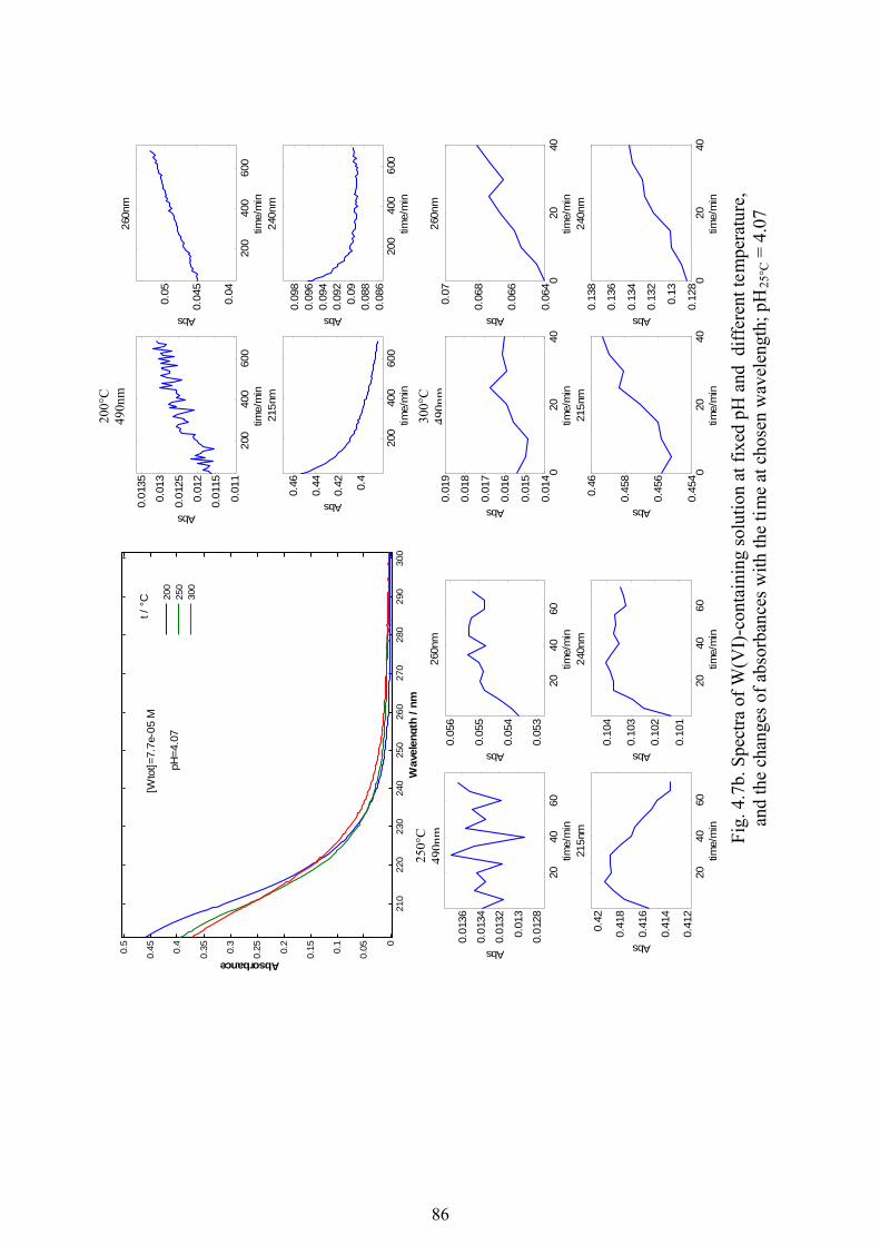
86
210
220
230
240
250
260
270
280
290
300
0
0.050.1
0.150.2
0.250.3
0.350.4
0.450.5
Wav
elen
gth
/nm
Absorbance
200
250
300
t/°C
[Wto
t]=7.
7e-0
5M
pH=4
.07
200
400
600
0.01
1
0.01
15
0.01
2
0.01
25
0.01
3
0.01
35
time/
min
Abs
200°
C32
0nm
200
400
600
0.04
0.04
5
0.05
time/
min
Abs
260n
m
200
400
600
0.4
0.42
0.44
0.46
time/
min
Abs
215n
m
200
400
600
0.08
60.
088
0.09
0.09
20.
094
0.09
60.
098
time/
min
Abs
240n
m
2040
600.
0128
0.01
3
0.01
32
0.01
34
0.01
36
time/
min
Abs
250°
C32
0nm
2040
600.
053
0.05
4
0.05
5
0.05
6
time/
min
Abs
260n
m
2040
600.
412
0.41
4
0.41
6
0.41
8
0.42
time/
min
Abs
215n
m
2040
60
0.10
1
0.10
2
0.10
3
0.10
4
time/
min
Abs
240n
m
020
400.
014
0.01
5
0.01
6
0.01
7
0.01
8
0.01
9
time/
min
Abs
300°
C32
0nm
020
400.
064
0.06
6
0.06
8
0.07
time/
min
Abs
260n
m
020
400.
454
0.45
6
0.45
8
0.46
time/
min
Abs
215n
m
020
400.
128
0.13
0.13
2
0.13
4
0.13
6
0.13
8
time/
min
Abs
240n
m
Fig.
4.7
b. S
pect
ra o
fW(V
I)-c
onta
inin
g so
lutio
n at
fixed
pH
and
diff
eren
t tem
pera
ture
,an
d th
e ch
ange
s of a
bsor
banc
es w
ith th
e tim
e at
cho
sen
wav
elen
gth;
pH
25°C
= 4
.07
200°
C
490n
m
300°
C
490n
m25
0°C
49
0nm
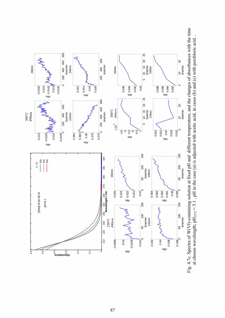
87
210
220
230
240
250
260
270
280
290
300
0
0.1
0.2
0.3
0.4
0.5
0.6
Wav
elen
gth
/nm
Absorbance
200
250
300
t/°C
[Wto
t]=8.
0e-0
5M
pH=5
.1
020
040
060
0-0
.014
5
-0.0
14
-0.0
135
-0.0
13
time/
min
Abs
200°
C32
0nm
020
040
060
080
0
0.01
35
0.01
4
0.01
45
0.01
5
0.01
55
time/
min
Abs
260n
m
020
040
060
080
00.
376
0.37
8
0.38
0.38
2
0.38
4
time/
min
Abs
215n
m
200
400
600
0.03
9
0.04
0.04
1
0.04
2
time/
min
Abs
240n
m
050
100
150
-0.0
11
-0.0
105
-0.0
1
-0.0
095
time/
min
Abs
250°
C32
0nm
050
100
150
0.02
0.02
1
0.02
2
0.02
3
0.02
4
time/
min
Abs
260n
m
050
100
150
0.43
6
0.43
8
0.44
0.44
2
time/
min
Abs
215n
m
050
100
150
0.05
9
0.06
0.06
1
0.06
2
0.06
3
0.06
4
time/
min
Abs
240n
m
510
1520
25-7
-6.5-6
-5.5-5
-4.5
x10
-3
time/
min
Abs
300°
C32
0nm
510
1520
250.
03
0.03
2
0.03
4
0.03
6
time/
min
Abs
260n
m
010
200.
516
0.51
8
0.52
0.52
2
0.52
4
time/
min
Abs
215n
m
010
20
0.09
2
0.09
4
0.09
6
0.09
8
time/
min
Abs
240n
m
Fig.
4.7
c. S
pect
ra o
fW(V
I)-c
onta
inin
g so
lutio
n at
fixe
d pH
and
diff
eren
t tem
pera
ture
, and
the
chan
ges o
f abs
orba
nces
with
the
time
at c
hose
nw
avel
engt
h; p
H25
°C=
5.1
, pH
in th
e ca
se (a
) is a
djus
ted
with
acet
icac
id,i
nca
ses(
b) a
nd (c
) with
per
chlo
ric a
cid.
.
250°
C
490n
m
200°
C
490n
m
300°
C
490n
m

88
a)
210 220 230 240 250 260 270 2800
0.05
0.1
0.15
0.2
0.25
0.3
0.35
0.4
Wavelength / nm
Abs
orba
nce
4.435.035.075.465.615.955.996.286.556.826.927.127.22
200°CpH
pH=5.61
pH=5.46
pH=7.22
b)
210 220 230 240 250 260 270 2800
0.05
0.1
0.15
0.2
0.25
0.3
0.35
0.4
Wavelength / nm
Abs
orba
nce
4.795.165.475.886.026.326.386.606.786.887.017.21
250°C pH
pH=7.21
pH=5.47
pH=5.88
Fig. 4.8. Spectra of W(VI) containing solutions, [Wtot] = 8x10⁻⁵ mol·dm-3:
(a) 200°C, (b) 250°C.
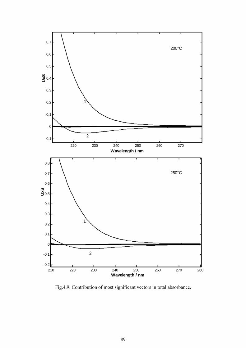
89
220 230 240 250 260 270
-0.1
0
0.1
0.2
0.3
0.4
0.5
0.6
0.7
Wavelength / nm
UxS
200°C
1
2
210 220 230 240 250 260 270 280-0.2
-0.1
0
0.1
0.2
0.3
0.4
0.5
0.6
0.7
0.8
Wavelength / nm
UxS
250°C
1
2
Fig.4.9. Contribution of most significant vectors in total absorbance.

90
210 220 230 240 250 260 270 2800
0.05
0.1
0.15
0.2
0.25
0.3
0.35
0.4spectra
210 220 230 240 250 260 270 280
-0.05
0
0.05
residuals
Wavelength / nm
Abs
orba
nce
200°C
210 220 230 240 250 260 270 2800
0.05
0.1
0.15
0.2
0.25
0.3
0.35
0.4
0.45
Wavelength / nm
Abs
orba
nce
spectra
210 220 230 240 250 260 270 280-0.1
-0.05
0
0.05
0.1residuals
250°C
Fig.4.10 Calculated (blue) and experimental (red) absorbances and their residuals at elevated
temperatures.

91
210 220 230 240 250 260 270 280
0
500
1000
1500
2000
2500
3000
3500
4000
4500
Wavelength / nm
Mol
arab
sorp
tivi
ty
200°C
250°C
Fig.4.11. Molar apsorptivities for the aqueous HWO4− (HL) and WO4
2- (L) species at elevated temperatures.

92
4.4. References
Aveston J., Anacker E. W., and Johnson J. S. (1964) Hydrolysis of molybdenum. VI. Ultracentrifugation, acidity measurements, and Raman spectra of polymolybdates. Inorg. Chem. 3(5), 735-46.
Bryzgalin O. V. (1976) Solubility of tungstic acid in aqueous saline solutions at high temperatures. Geokhimiya 6, 864-870.
Bryzgalin O. V. (1983) Instability constants of tungsten hydroxy-complexes at high temperatures (based on an electrostatic model). Geokhimiya(2), 228-35.
Dickson A. G., Wesolowski D. J., Palmer D. A., and Mesmer R. E. (1990) Dissociation constant of bisulfate ion in aqueous sodium chloride solutions to 250°C. Journal of Physical Chemistry 94(12), 7978-7985.
Fernandez D. P., Goodwin A. R. H., Lemmon E. W., Sengers J. M. H. L., and Williams R. C. (1997) A formulation for the static permittivity of water and steam at temperatures from 238 K to 873 K at pressures up to 1200 MPa, including derivatives and Debye-Hueckel coefficients. Journal of Physical and Chemical Reference Data 26(4), 1125-1166.
Foster R. P. (1977) Solubility of scheelite in hydrothermal chloride solutions. Chemical Geology 20(1), 27-43.
Ivanova G. F. and Khodakovskii I. L. (1968) Tungsten migration forms in hydrothermal solutions. Geokhimiya 8, 930-940.
Jander G., Mojert D., and Aden T. (1929) Amphoteric hydroxides, their aqueous solutions and crystalline compounds. VIII. Z. anorg. allgem. Chem. 180, 129-49.
Mesmer R. E., Patterson C. S., Busey R. H., and Holmes H. F. (1989) Ionization of acetic acid in aq. sodium chloride media: a potentiometric study to 573K and 130 bar. Journal of Physical Chemistry 93(21), 7483-90.
Sasaki Y. (1961) Equilibrium studies of polyanions. The first step in the acidification of WO4
2-; equilibriums in 3M NaClO4 at 25°C. Acta Chemica Scandinavica 15, 175-89. Schwarzenbach G. and Meier J. (1958) Formation and investigation of unstable protonation
and deprotonation products of complexes in aqueous solution. Journal of Inorganic and Nuclear Chemistry 8, 302-12.
Shock E. L. and Koretsky C. M. (1993) Metal-organic complexes in geochemical processes: calculation of standard partial molal thermodynamic properties of aqueous acetate complexes at high pressures and temperatures. Geochimica et Cosmochimica Acta 57(20), 4899-922.
Spitsyn V. I. and Kabanov V. Y. (1960) Investigation of the mechanism of formation of high-molecular-weight tungsten compounds by dilatometric and spectrophotometric methods. Doklady Akademii Nauk SSSR 132, 1114-17.
Suleimenov O. M. (2004) Simple, compact, flow-through, high temperature high pressure cell for UV-Vis spectrophotometry. Review of Scientific Instruments 75(10, Pt. 1), 3363-3364.
Tytko K. H. and Glemser O. (1976) Isopolymolybdates and isopolytungstates. Advances in Inorganic Chemistry and Radiochemistry 19, 239-315.
Wagner W. (1998) Properties of Water and Steam/The Industrial Standard IAPWS-IF97 for the Thermodynamic Properties and Supplementary Equations for Other Properties.
Wesolowski D., Drummond S. E., Mesmer R. E., and Ohmoto H. (1984) Hydrolysis Equilibria of Tungsten(VI) in Aqueous Sodium Chloride Solutions to 300°C. Inorganic Chemistry 23(8), 1120-1132.
93
Wood S. A. and Vlassopoulos D. (1989) Experimental determination of the hydrothermal solubility and speciation of tungsten at 500°C and 1 kbar. Geochimica et Cosmochimica Acta 53(2), 303-312.
Wood S. A. (1992) Experimental determination of the solubility of tungstate(s) and the thermodynamic properties of H2WO4(aq) in the range 300-600°C at 1 kbar: calculation of scheelite solubility. Geochimica et Cosmochimica Acta 56(5), 1827-1836.
Wood S. A. and Samson I. M. (2000) The hydrothermal geochemistry of tungsten in granitoid environments: I. Relative solubilities of ferberite and scheelite as a function of T, P, pH, and mNaCl. Economic Geology and the Bulletin of the Society of Economic Geologists 95(1), 143-182.
Yastrebova L. F., Borina A. F., and Ravich M. I. (1963) Solubility of calcium molybdate and tungstate in aqueous solutions of potassium and sodium chlorides at high temperatures. Zhurnal Neorganicheskoi Khimii 8, 208-17.
Yatsimirskii K. B. and Prik K. E. (1964) Catalytic oxidation of iodide ion with hydrogen peroxide in the presence of tungsten(VI). Zhurnal Neorganicheskoi Khimii 9(8), 1838-43.
Yatsimirskii K. B. and Romanov V. F. (1965) Kinetics and mechanism for the oxidation of p-phenylenediamine with potassium iodate in the presence of tungsten(VI) compounds. Zhurnal Neorganicheskoi Khimii 10(7), 1607-12.

94
4.4. Appendix Appendix 4.4.1. Initial composition of the W(VI)-containing solutions for the experiments at
ambient temperature.
Set I.
Wtot Natot ClO4 tot pH
1 9.94E-05 1.99E-04 2.90E-06 5.54
2 9.92E-05 1.98E-04 6.15E-06 5.21
3 9.88E-05 1.98E-04 1.24E-05 4.91
4 9.79E-05 1.96E-04 2.44E-05 4.61
5 9.66E-05 1.93E-04 4.35E-05 4.36
6 9.94E-05 1.99E-04 8.33E-05 4.08
7 9.93E-05 1.99E-04 1.35E-04 3.87
8 9.90E-05 1.98E-04 2.34E-04 3.63
9 9.87E-05 1.97E-04 3.70E-04 3.43
10 9.75E-05 1.95E-04 8.15E-04 3.09
11 9.65E-05 1.93E-04 1.21E-03 2.92
12 9.93E-05 1.99E-04 2.96E-03 2.53
13 9.86E-05 1.97E-04 7.97E-03 2.10
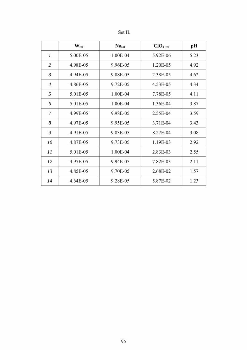
95
Set II.
Wtot Natot ClO4 tot pH
1 5.00E-05 1.00E-04 5.92E-06 5.23
2 4.98E-05 9.96E-05 1.20E-05 4.92
3 4.94E-05 9.88E-05 2.38E-05 4.62
4 4.86E-05 9.72E-05 4.53E-05 4.34
5 5.01E-05 1.00E-04 7.78E-05 4.11
6 5.01E-05 1.00E-04 1.36E-04 3.87
7 4.99E-05 9.98E-05 2.55E-04 3.59
8 4.97E-05 9.95E-05 3.71E-04 3.43
9 4.91E-05 9.83E-05 8.27E-04 3.08
10 4.87E-05 9.73E-05 1.19E-03 2.92
11 5.01E-05 1.00E-04 2.83E-03 2.55
12 4.97E-05 9.94E-05 7.82E-03 2.11
13 4.85E-05 9.70E-05 2.68E-02 1.57
14 4.64E-05 9.28E-05 5.87E-02 1.23
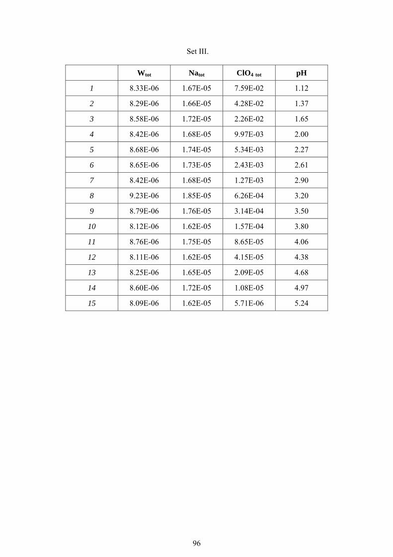
96
Set III.
Wtot Natot ClO4 tot pH
1 8.33E-06 1.67E-05 7.59E-02 1.12
2 8.29E-06 1.66E-05 4.28E-02 1.37
3 8.58E-06 1.72E-05 2.26E-02 1.65
4 8.42E-06 1.68E-05 9.97E-03 2.00
5 8.68E-06 1.74E-05 5.34E-03 2.27
6 8.65E-06 1.73E-05 2.43E-03 2.61
7 8.42E-06 1.68E-05 1.27E-03 2.90
8 9.23E-06 1.85E-05 6.26E-04 3.20
9 8.79E-06 1.76E-05 3.14E-04 3.50
10 8.12E-06 1.62E-05 1.57E-04 3.80
11 8.76E-06 1.75E-05 8.65E-05 4.06
12 8.11E-06 1.62E-05 4.15E-05 4.38
13 8.25E-06 1.65E-05 2.09E-05 4.68
14 8.60E-06 1.72E-05 1.08E-05 4.97
15 8.09E-06 1.62E-05 5.71E-06 5.24

97
Set IV.
Wtot Natot ClO4 tot pH
1 2.89E-06 5.78E-06 5.22E-06 5.28
2 2.76E-06 5.52E-06 8.14E-06 5.09
3 2.80E-06 5.61E-06 1.39E-05 4.86
4 2.86E-06 5.72E-06 2.17E-05 4.66
5 2.88E-06 5.77E-06 3.42E-05 4.47
6 2.96E-06 5.93E-06 5.16E-05 4.29
7 2.84E-06 5.69E-06 8.70E-05 4.06
8 2.91E-06 5.82E-06 1.40E-04 3.85
9 2.72E-06 5.44E-06 2.18E-04 3.66
10 2.96E-06 5.93E-06 3.52E-04 3.45
11 2.86E-06 5.72E-06 5.67E-04 3.25
12 2.72E-06 5.43E-06 8.73E-04 3.06
13 2.98E-06 5.96E-06 1.67E-03 2.78
14 2.80E-06 5.59E-06 3.42E-03 2.47
15 2.83E-06 5.67E-06 6.87E-03 2.16
16 2.84E-06 5.67E-06 1.37E-02 1.86
17 2.89E-06 5.78E-06 2.69E-02 1.57
18 2.80E-06 5.60E-06 5.49E-02 1.26
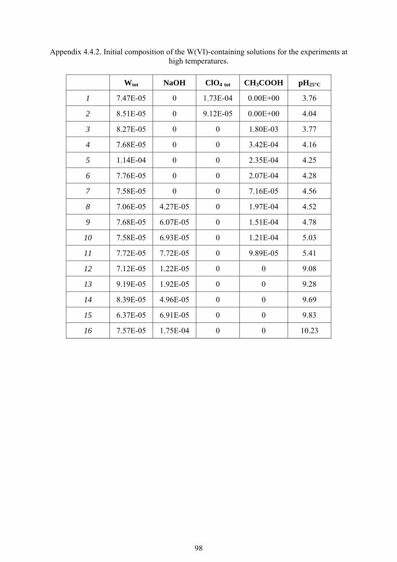
98
Appendix 4.4.2. Initial composition of the W(VI)-containing solutions for the experiments at high temperatures.
Wtot NaOH ClO4 tot CH3COOH pH25°C
1 7.47E-05 0 1.73E-04 0.00E+00 3.76
2 8.51E-05 0 9.12E-05 0.00E+00 4.04
3 8.27E-05 0 0 1.80E-03 3.77
4 7.68E-05 0 0 3.42E-04 4.16
5 1.14E-04 0 0 2.35E-04 4.25
6 7.76E-05 0 0 2.07E-04 4.28
7 7.58E-05 0 0 7.16E-05 4.56
8 7.06E-05 4.27E-05 0 1.97E-04 4.52
9 7.68E-05 6.07E-05 0 1.51E-04 4.78
10 7.58E-05 6.93E-05 0 1.21E-04 5.03
11 7.72E-05 7.72E-05 0 9.89E-05 5.41
12 7.12E-05 1.22E-05 0 0 9.08
13 9.19E-05 1.92E-05 0 0 9.28
14 8.39E-05 4.96E-05 0 0 9.69
15 6.37E-05 6.91E-05 0 0 9.83
16 7.57E-05 1.75E-04 0 0 10.23

99
Appendix 4.4.3. Molar absorptivities of the components of background absorbance.
190 200 210 220 230 240 250 260 270 2800
500
1000
1500
2000
2500
3000
Wavelength / nm
Mol
ar a
bsor
ptiv
ity
25 50 75100150200250300
t / °C
300°C
25°C
.Molar absorptivities of OH − at different temperatures and saturated water vapour pressures.
210 220 230 240 250 260 2700
200
400
600
800
1000
Wavelength / nm
Mol
ar a
bsor
ptiv
ity
CH3COOHCH3COO -
..........._____
Molar absorptivities of CH3COOH and CH3COO − at 200°C (red) and 250°C (green) and
saturated water vapour pressure.

100
5. Acridinium ion ionisation at elevated temperatures and pressures to 200°C and 2000 bar
5.1 .Introduction
In the fields of corrosion science, chemical processing and synthesis as well as
geochemistry, it is of interest to be able to measure the thermodynamic properties of aqueous
solutions under extreme conditions of temperature and pressure. One such property is pH at
hydrothermal conditions. Thermally stable indicators have gained some popularity in recent
years due to the possibility of being able to measure pH directly in situ when the
conventional methods, such as for example, potentiometry, have suffered limitations (i.e.
limited temperature range for glass electrodes, lower precision for high-temperature ceramic
electrodes etc.). There have been a number of previous studies carried out on temperature
dependence of ionisation of widely used indicators such as methyl orange (BOLTON et al.,
1973; BOILY and SEWARD, 2005), bromphenol blue (PAVLYUK and SMOLYAKOV, 1974a),
thymol blue (YAMAZAKI et al., 1992), 2-naphtol (XIANG and JOHNSTON, 1994), 2,5-
dinitrophenol (LEE et al., 1994), p- and o-nitrophenols (PAVLYUK and SMOLYAKOV, 1974b).
Acridine is of particular interest because of its thermal stability (LEE et al., 1992; HUH et al.,
1993; RYAN et al., 1997). Previous studies have employed different methods (e.g. uv-vis
spectroscopy (HUH et al., 1993; RYAN et al., 1997; ROS et al., 1998), fluorescence
spectroscopy (ROSENBERG et al., 1979; RYAN et al., 1997), capillary electrophoresis (JIA et
al., 2001) to measure the protonation equilibrium of acridine up to 380°C and 240 bar. There
is a difference of up to 0.2 in the reported values of pK for acridine ionisation (table 5.1) and
this extends to the values reported high temperatures by Huh et al.(1993) and Ryan et
al.(1997). The aim of this study has therefore been to re-examine the temperature
dependence of acridine ionisation up to 200°C at equilibrium saturated vapour pressures as
well as to study the effect of pressure up to 2000 bar.
Fig.5.1. Protonation of acridine in acid solutions.
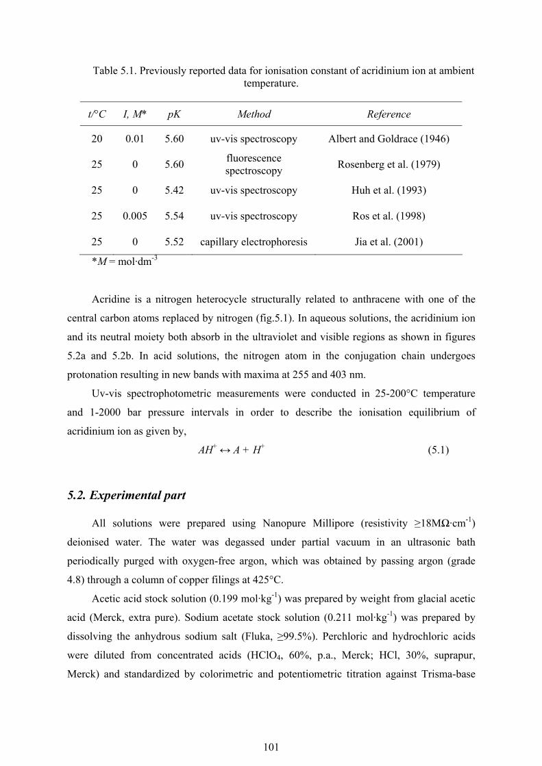
101
Table 5.1. Previously reported data for ionisation constant of acridinium ion at ambient temperature.
t/°C I, M* pK Method Reference
20 0.01 5.60 uv-vis spectroscopy Albert and Goldrace (1946)
25 0 5.60 fluorescence spectroscopy Rosenberg et al. (1979)
25 0 5.42 uv-vis spectroscopy Huh et al. (1993)
25 0.005 5.54 uv-vis spectroscopy Ros et al. (1998)
25 0 5.52 capillary electrophoresis Jia et al. (2001)
*M = mol·dm-3
Acridine is a nitrogen heterocycle structurally related to anthracene with one of the
central carbon atoms replaced by nitrogen (fig.5.1). In aqueous solutions, the acridinium ion
and its neutral moiety both absorb in the ultraviolet and visible regions as shown in figures
5.2a and 5.2b. In acid solutions, the nitrogen atom in the conjugation chain undergoes
protonation resulting in new bands with maxima at 255 and 403 nm.
Uv-vis spectrophotometric measurements were conducted in 25-200°C temperature
and 1-2000 bar pressure intervals in order to describe the ionisation equilibrium of
acridinium ion as given by,
AH+ ↔ A + H+ (5.1)
5.2. Experimental part
All solutions were prepared using Nanopure Millipore (resistivity ≥18MΩ·cm-1)
deionised water. The water was degassed under partial vacuum in an ultrasonic bath
periodically purged with oxygen-free argon, which was obtained by passing argon (grade
4.8) through a column of copper filings at 425°C.
Acetic acid stock solution (0.199 mol·kg-1) was prepared by weight from glacial acetic
acid (Merck, extra pure). Sodium acetate stock solution (0.211 mol·kg-1) was prepared by
dissolving the anhydrous sodium salt (Fluka, ≥99.5%). Perchloric and hydrochloric acids
were diluted from concentrated acids (HClO4, 60%, p.a., Merck; HCl, 30%, suprapur,
Merck) and standardized by colorimetric and potentiometric titration against Trisma-base

102
a)
250 300 350 400 450
0
0.1
0.2
0.3
0.4
0.5
Wavelength / nm
Abs
orba
nce
AH
A
+
25°C
b)
320 340 360 380 400 420 440 4600
0.1
0.2
0.3
0.4
0.5
0.6
0.7
0.8
0.9
1
Wavelength / nm
Abs
orba
nce
A
AH+ 25°C
Fig.5.2. Spectra of acridine and acridinium ion at 25°C corrected for background absorbance: a) over the whole range of studied wavelengths, [A] =3.27×10⁻⁶ mol·kg-1 and
[AH+] =3.96×10⁻⁶ mol·kg-1, b) details of the fine structure of the absorption spectrum in the visible region, [A] =5.1×10⁻⁵ mol·kg-1 and [AH+] =5.17×10⁻⁵ mol·kg-1.

103
(Tris(hydroxymethyl)aminomethane, 99+%, Aldrich) using methyl red as indicator. Sodium
hydroxide solution (0.082 mol·kg-1) was diluted from saturated sodium hydroxide solution
(50% solution in water, Aldrich) with CO2-free water and standardized under argon pressure
slightly above atmospheric by potentiometric and colorimetric titration against standardized
perchloric acid (using methyl red as an indicator). The prepared solution was stored in a
flask connected with a glass tube filled with ascarite (Fluka, 5-20mesh) and drierite (Fluka,
+4 mesh) in order to keep it CO2-free. The pH of the studied solutions was maintained by
various combinations of the above mentioned reagents. The pH was measured at
atmospheric pressure and room temperature with a glass combination electrode (Metrohm),
calibrated every day against at least 2 standard buffer solutions.
Acridine (Aldrich, 97%) was purified by recrystallization from ethanol and dried at
100°C until a constant weight was attained. Because of the very low solubility in pure water,
stock solutions of acridine were prepared by dissolution in dilute acid. The acridine solutions
were prepared with degassed (deoxygenated) water as mentioned above in order to avoid
oxidation, especially at elevated temperatures (LEE et al., 1992). Prepared stock solutions of
acridine were stored under argon and protected from light. Freshly diluted solutions were
prepared prior to each experiment and degassed and purged with deoxygenated argon just
before the measurements were made.
Initially, it was decided to study the spectra of acridine in perchloric acid solutions. A
stock solution of acridine (2.2 mmol·kg-1) in 0.063 mol·kg-1 perchloric acid was prepared.
However, after one week of storage, the solution had changed from lemon yellow to dark
yellow and long, acicular orange crystals began to precipitate. In addition, the spectrum of
acridine dissolved in the perchloric acid solution was observed to change over a period of 30
minutes at 25°C. The oxidation of acridine by perchloric acid therefore precluded the use of
the latter to define and adjust pH in our experiments. More dilute (~0.3-0.5 mmol·kg-1)
acridine stock solutions prepared with acetic acid appeared to be stable and no precipitates
were observed in solutions stored for up to a month. Spectra of solutions, in which pH was
adjusted with hydrochloric and acetic acid, acetate and sodium hydroxide, showed no change
over 30 min at any studied temperature and pressure in contrast to the observation of
Bulemela et al. (2005) who noted that absorbance of acridine during the experiment was
decreasing by 0.9 percent-per-min at both at 25 and 250°C.
Two independent series of experiments were conducted in order to determine the
temperature and pressure dependence of acridinium ion ionisation.
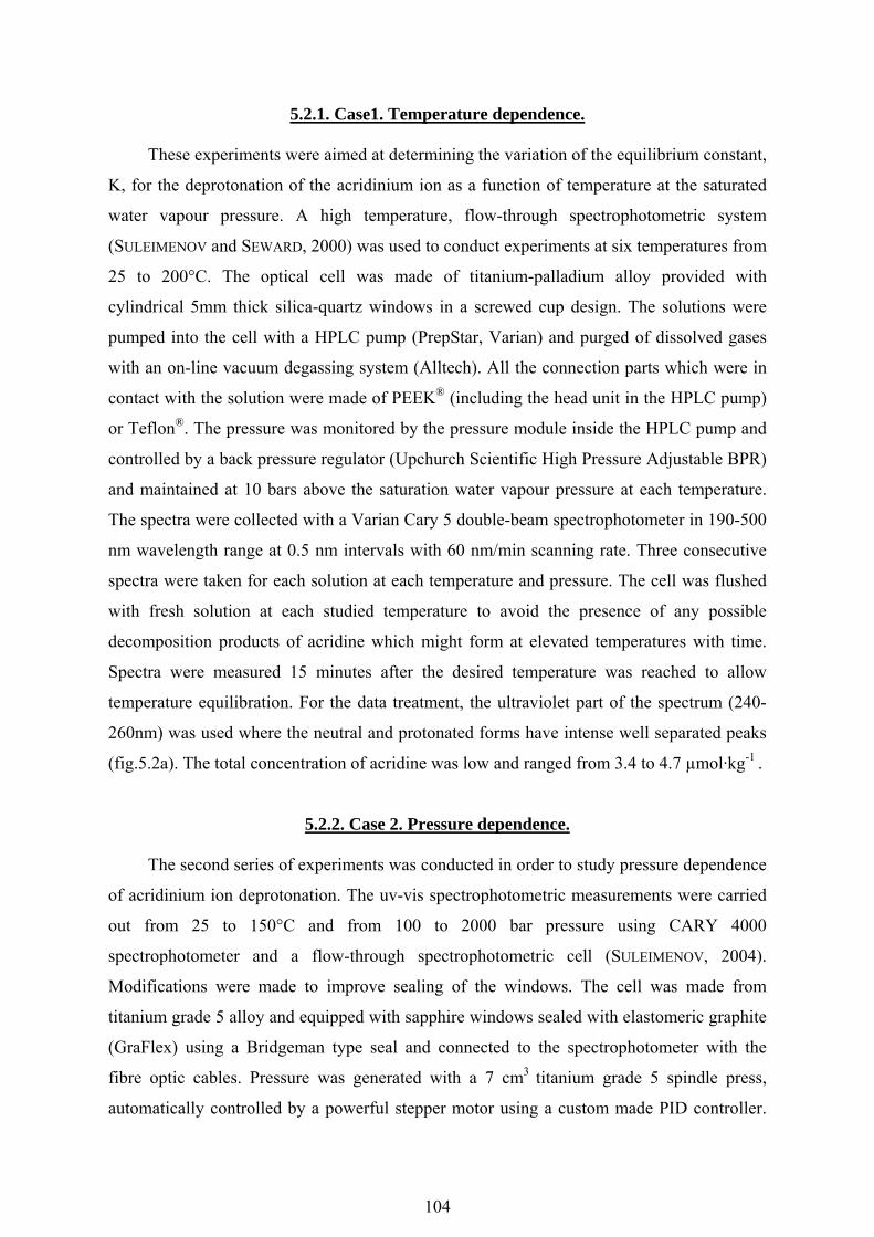
104
5.2.1. Case1. Temperature dependence.
These experiments were aimed at determining the variation of the equilibrium constant,
K, for the deprotonation of the acridinium ion as a function of temperature at the saturated
water vapour pressure. A high temperature, flow-through spectrophotometric system
(SULEIMENOV and SEWARD, 2000) was used to conduct experiments at six temperatures from
25 to 200°C. The optical cell was made of titanium-palladium alloy provided with
cylindrical 5mm thick silica-quartz windows in a screwed cup design. The solutions were
pumped into the cell with a HPLC pump (PrepStar, Varian) and purged of dissolved gases
with an on-line vacuum degassing system (Alltech). All the connection parts which were in
contact with the solution were made of PEEK® (including the head unit in the HPLC pump)
or Teflon®. The pressure was monitored by the pressure module inside the HPLC pump and
controlled by a back pressure regulator (Upchurch Scientific High Pressure Adjustable BPR)
and maintained at 10 bars above the saturation water vapour pressure at each temperature.
The spectra were collected with a Varian Cary 5 double-beam spectrophotometer in 190-500
nm wavelength range at 0.5 nm intervals with 60 nm/min scanning rate. Three consecutive
spectra were taken for each solution at each temperature and pressure. The cell was flushed
with fresh solution at each studied temperature to avoid the presence of any possible
decomposition products of acridine which might form at elevated temperatures with time.
Spectra were measured 15 minutes after the desired temperature was reached to allow
temperature equilibration. For the data treatment, the ultraviolet part of the spectrum (240-
260nm) was used where the neutral and protonated forms have intense well separated peaks
(fig.5.2a). The total concentration of acridine was low and ranged from 3.4 to 4.7 µmol·kg-1 .
5.2.2. Case 2. Pressure dependence.
The second series of experiments was conducted in order to study pressure dependence
of acridinium ion deprotonation. The uv-vis spectrophotometric measurements were carried
out from 25 to 150°C and from 100 to 2000 bar pressure using CARY 4000
spectrophotometer and a flow-through spectrophotometric cell (SULEIMENOV, 2004).
Modifications were made to improve sealing of the windows. The cell was made from
titanium grade 5 alloy and equipped with sapphire windows sealed with elastomeric graphite
(GraFlex) using a Bridgeman type seal and connected to the spectrophotometer with the
fibre optic cables. Pressure was generated with a 7 cm3 titanium grade 5 spindle press,
automatically controlled by a powerful stepper motor using a custom made PID controller.

105
The pressure was measured with a strain gauge pressure transducer calibrated against a
Heise® Bourdon tube pressure gauge. Before each measurement, the cell was flushed with
fresh solution (i.e. at each studied temperature). For the data treatment, the visible part of the
spectra (320-450 nm) was used (fig.5.2b). Since the absorbance in this region is less intense
than in the ultraviolet region, the solutions analysed in a cell with sapphire windows were 5
to 10 times more concentrated (i.e. in the range from 2.5 to 8.3 µmol·kg-1 ) than the solutions
studied at the equilibrium saturated vapour pressures (i.e. case 1).
5.3. Data treatment. The collected spectra were stored in an absorbance matrix Ai×j, where i=number of
wavelengths, j = number of analysed solutions. Water, sodium hydroxide, acetic acid and
sodium acetate baseline spectra were measured separately at the temperatures studied. The
acridine spectra were corrected for background absorbance (i.e. windows plus solvent). In
order to determine the number of absorbing species (rank or number of principal
components) required for a chemical model, we used singular value decomposition (SVD):
Ai×j = U i×n × S n×n × V j×n T (5.2)
where the matrixes U, S, V are the result of singular value decomposition of matrix A, U is
the i×n matrix of left singular vectors that form an orthonormal basis for the absorption
profile, S is the n×n diagonal matrix of singular values, and V is the n×j matrix of right
singular values, that form an orthonormal basis for the concentration dependence response.
By convention, the ordering of the singular vectors is determined by high-to-low sorting of
singular values, with the highest singular value in the upper left index of the matrix. One
important result of the singular value decomposition of A is that
A(l) =∑ U k × S k × V T k (5.3)
is the closest rank-l matrix to our original absorbance matrix Ai×j, (i.e. A(l) minimizes the
sum of the squares of the difference of the elements of A and A(l)) . In fig.5.3, one can see
the product of U and S matrices plotted versus wavelength, indicating the contribution of the
most significant vectors to the absorption profile. Such a procedure was repeated for each
studied temperature and demonstrated that only 2 vectors are representing more than 99% of
the raw absorption data and all the rest are randomly oscillating around zero and therefore
were discarded, as most probably corresponding to random instrumental noise and small
imprecision in solution preparation.

106
246 248 250 252 254 256 258 260-1
-0.8
-0.6
-0.4
-0.2
0
0.2
0.4
Wavelength / nm
US
2
1
25°C
246 248 250 252 254 256 258 260-0.2
0
0.2
0.4
0.6
0.8
1
1.2
Wavelength / nm
US
1
2
200°C
Fig 5.3. The contribution of most significant vectors in total absorbance.
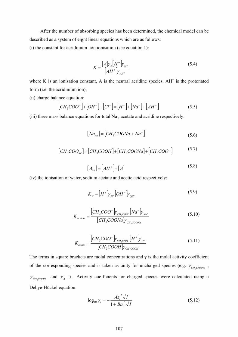
107
After the number of absorbing species has been determined, the chemical model can be
described as a system of eight linear equations which are as follows:
(i) the constant for acridinium ion ionisation (see equation 1):
[ ] [ ][ ] +
+
+
+
=AH
HA
AHHA
Kγγγ (5.4)
where K is an ionisation constant, A is the neutral acridine species, AH+ is the protonated
form (i.e. the acridinium ion);
(ii) charge balance equation:
[ ] [ ] [ ] [ ] [ ] [ ]+++−−− ++=++ AHNaHClOHCOOCH3 (5.5)
(iii) three mass balance equations for total Na , acetate and acridine respectively:
[ ] [ ]++= NaCOONaCHNatot 3 (5.6)
[ ] [ ] [ ] [ ]−++= COOCHCOONaCHCOOHCHCOOCH tot 3333 (5.7)
[ ] [ ] [ ]AAHAtot += + (5.8)
(iv) the ionisation of water, sodium acetate and acetic acid respectively:
[ ] [ ] −+−+=
OHHw OHHK γγ (5.9)
[ ] [ ][ ]
COONaCH
NaCOOCHacetate COONaCH
NaCOOCHK
3
3
3
3
γ
γγ +−+−
= (5.10)
[ ] [ ][ ] COOHCH
HCOOCHacetic COOHCH
HCOOCHK
3
3
3
3
γ
γγ +−+−
= (5.11)
The terms in square brackets are molal concentrations and γ is the molal activity coefficient
of the corresponding species and is taken as unity for uncharged species (e.g. COONaCH3
γ ,
COOHCH3γ and
Aγ ) . Activity coefficients for charged species were calculated using a
Debye-Hückel equation:
IBaIAz
i
ii 0
2
10 1log
+−=γ (5.12)

108
where the Debye-Hückel limiting slope parameters A, B, as a function of temperature and
pressure, were taken from (FERNANDEZ et al., 1997). The maximum ionic strength in all
solutions was always ≤0.02 mol·dm-3 and generally <0.001 mol·dm-3. The iterative
calculation procedure was based on successive substitution with the initial assumption that
all the activity coefficients were equal to unity.
The calculations were carried out on the molal scale and conversion to the molar units
of Beer’s law was facilitated using the temperature dependent density data for water (given
the low concentration of acridine). The densities of pure water at different temperatures and
pressures were calculated according to the Haar-Gallagher-Kell (HGK) model as given in
Kestin et al.(1984) The relevant values for the ion product constant of water, Kw, as a
function of temperature and pressure were taken from Marshall and Franck (1981). The ion
pair constants for sodium acetate and sodium hydroxide association were taken from Shock
and Koretsky (1993) and Ho and Palmer (1996) , respectively. However, for the dilute
solutions and temperatures and pressures studied, the formation of sodium acetate and
hydroxide ion pairs is negligible. Their inclusion in the computational scheme contributed
only to the third decimal place of acridine ionisation pK at 200°C (less at the higher
pressures) which is much smaller than the experimental error. The values for pK for acetic
acid up to 200°C at the saturated vapour pressure were taken from the precise conductivity
data of Ellis (1963) which are identical to the “smoothed” literature compilation given by
Mesmer et al (1989). The pressure dependence of ionisation of acetic acid was taken from
the conductivity study of Lown et al. (1970) which gives values of the equilibrium constant
up to 225°C and 3000 bar.
The pK of acridinium ion deprotonation was obtained using following equation:
ε×C = A = U i×n × S n×n × V j×n T (5.13)
where the left part of the equation represents Beer’s law in which ε is the i×n matrix of
molar absorptivities and C is the n×j matrix of molar concentrations of absorbing species.
Matrix C is obtained from the solution of the system of eight linear equations describing the
chosen chemical model (see above). The right part of the equation is the SVD of the
absorbance matrix, A, with n absorbing species (n=2). The calculation procedure involving
matrix manipulations using Matlab 7.0 and Maple 8 computational platforms is described in
detail elsewhere (BOILY and SULEIMENOV, 2006).

109
5.4. Results and discussion The spectra of neutral acridine and its protonated form over the whole range of
studied wavelengths at 25°C are shown in fig.5.2 . In the uv region from 200-270 nm, the
maximum of absorbance for acridinium ion occurs at 255nm and for acridine at 249.5nm,
while in visible region, the intensity of absorbance is much smaller with the maxima at 355
and 356 nm for acridinium ion and acridine respectively with an additional peak for
acridinium ion occurring at 403 nm.
5.4.1. Case 1. Temperature dependence.
The spectra of acridine at different values of pH are shown in fig.5.4. At pH=3.87,
the spectrum is due predominantly to the HA+ species. With increasing pH, the formation of
the deprotonated (neutral) acridine (A) proceeds such that at pH=9.95, the spectrum is due to
the neutral species.
240 245 250 255 260 265 2700
0.1
0.2
0.3
0.4
0.5
0.6
0.7
0.8
0.9
1
Wavelength / nm
Abs
orba
nce
pH=9.95
6.45
5.66
3.86
4.44
5.03
5.66
6.45
9.95
Fig.5.4. Absorbance of acridine aqueous solutions at 25°C as a function of pH for Acrtot = from 3.4 ×10⁻⁶ to 4.6×10⁻⁶ mol·kg-1.
The maximum in the absorbance of neutral acridine occurs in the ultraviolet region and
remains at 249.5 nm with increasing temperature up to 150°C (fig.5.5a). At 200°C, the band
maximum undergoes a weak blue shift to 249.0 nm, while for acridinium ion absorbance, the
maximum undergoes a weak red shift from 255.0 to 256.0 nm (fig.5.5b) over
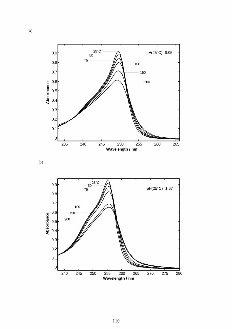
110
a)
235 240 245 250 255 260 2650
0.1
0.2
0.3
0.4
0.5
0.6
0.7
0.8
0.9
Wavelength / nm
Abs
orba
nce
25°C50
75100
150
200
pH(25°C)=9.95
b)
240 245 250 255 260 265 270 275 2800
0.1
0.2
0.3
0.4
0.5
0.6
0.7
0.8
0.9
Wavelength / nm
Abs
orba
nce
pH(25°C)=1.6725°C
5075
100
150
200

111
c)
220 230 240 250 260 270 2800
0.1
0.2
0.3
0.4
0.5
0.6
Wavelength / nm
Abs
orba
nce
25°C50
75
100
150
200
pH(25°C)=3.86
Fig.5.5. Spectra of acridine aqueous solutions at different temperatures: (a) pH=9.95, Acr tot =3.38×10⁻⁶ mol·kg-1; (b) pH=1.67, Acr tot =4.77×10⁻⁶ mol·kg-1;
(c) pH=3.86, Acr tot =3.44×10⁻⁶ mol·kg-1.
240 245 250 255 260 265 270 275 2800
2
4
6
8
10
12
14
16
x 104
Wavelength / nm
Mol
ar a
bsor
ptiv
ity
25°C200°CA
AH+
Fig.5.6. Molar absorptivities of acridine and acridinium ion at 25 and 200°C .

112
the 25-200°C temperature range. The spectra of both species (A and AH+) in the visible
region undergo a small red shift with increasing temperature to 200°C (i.e. 355.0 to 356.0
nm for A and from 354 to 355.5 nm for AH+). Increasing temperature causes significant
changes in the absorption spectrum of a solution which initially contains more than 98% of
fully protonated acridine species at 25°C and pH25°C=3.85 (fig.5.5c), as a result of increasing
of ionisation of acridinium ion. The molar absorptivities of both species at 25 and 200°C are
shown in fig. 5.6.
The values of ionisation constants for acridinium ion at different temperatures are
shown in the table 5.2 and are plotted together with available literature data in fig. 5.7. Our
pK values at 25° and 50°C are in perfect agreement with those reported by Ros (1998) and
Jia (2001), while the high temperature data of Huh (1993), as well as Ryan et al. (1997)
(both derived by uv-vis methods) are lower at each studied temperature by about 0.1 and 0.2
log units, respectively. The reason for this is not clear. The uncertainties in pK were
evaluated using a Monte Carlo simulation of experimental errors arising from solution
preparation, temperature and absorbance. The influence of temperature uncertainty on the
density of water and ionisation constants of acetic acid, sodium acetate and water as well as
solution preparation were evaluated separately by the same principle using 10000 iterations
based on a Monte Carlo method.
Table 5.2. Temperature dependence of equilibrium ionisation constant of acridinium ion with 2 sigma confidence interval calculated by Monte Carlo method given in parentheses
(see text).
t/°C log10K (±2σ)
25 -5.52 (±0.02)
50 -5.15 (±0.02)
75 -4.85 (±0.02)
100 -4.56 (±0.03)
150 -4.17 (±0.04)
200 -3.74 (±0.04)

113
0 50 100 150 200 2503
3.5
4
4.5
5
5.5
6
Temperature / °C
pK
Huh et al.,1993Ryan et al,1997Rosenberg et al.,1979Jia et al.,2001Ros et al.,1998This study/in quartz at Psat.,240-260nmwas used for data treatmentThis study/in saphire at 100bar,370-420nm was used for data treatment
Fig.5.7. Temperature dependence of ionisation constant of acridiniuim ion compared with available literature data.
Fig 5.8. Van’t Hoff plot for the ionisation constant of acridinium ion. (experimental values obtained at saturated vapour pressure and linear fit with the R2value).

114
Since the ionisation reaction of acridinium ion is isocoulombic (eq.5.1), the
dependence of log10K vs 1/T is expected to be close to linear (fig. 5.8). Linearity of this plot
also indicates that ΔCp≈0 for the reaction and that the dependence log10K versus T could be
described with a classic van’t Hoff equation :
TbaK +=10log (5.14)
where a = -0.78794 and b = -1411.767 .
Equation 5.14 was differentiated with respect to the temperature in order to obtain the
enthalpy (ΔH0) and entropy (ΔS0) for the acridine deprotonation:
dTKRT
TTG
Hp
ln)/1(
)/( 20
0 ∂=⎟
⎟⎠
⎞⎜⎜⎝
⎛
∂
Δ∂=Δ (5.15)
and
pTGS ⎟⎟
⎠
⎞⎜⎜⎝
⎛∂Δ∂
−=Δ0
0 (5.16)
Over the temperature range studied up to 200°C and at the equilibrium saturated vapour
pressure, the ionisation of acridine is characterised by an endothermic enthalpy (∆H0 =
+27.01 kJ/mol) and small negative entropy (∆S0 = -15.08 J/mole·K).
5.4.2. Case 2. Pressure dependence.
Figure 5.9 shows the measured spectra of acridine-containing solutions at different
pressures at 50°C. The increase of absorbance is mainly due to higher molar concentration
of acridine with increasing pressure because of decrease in volume by compressing the
solution. No shift in band position with increasing pressure was detected in either basic or
acid solutions.
The effect of pressure on the acridinium ion ionisation constant with increasing
temperature to 150°C is given in the table 5.3 and figure 5.10. The pressure dependence of
acridinium ion ionisation is very small over the studied temperature interval. The change in
partial molar volume for the ionisation reaction (∆V) and molar compressibility change (∆k)
can be evaluated with the following equations:
TT PKRT
PGV ⎟
⎠⎞
⎜⎝⎛
∂∂
−=⎟⎟⎠
⎞⎜⎜⎝
⎛∂∂
=Δln0
(5.17)
kPV
T
Δ−=⎟⎠⎞
⎜⎝⎛∂Δ∂ (5.18)

115
Since the values of pK are constant at each temperature over the studied pressure
interval (all changes in pK with pressure are within experimental error), ∆V is considered to
be constant with a value of 0.0 ± 1.2 cm3·mol-1. It follows that the partial molar
compressibility is therefore zero. Such a small pressure effect is characteristic also for
imidazol, another heterocyclic compound, whose pK is “insensitive” to increasing pressure
up to 6000 bar (TSUDA et al., 1976).
Since the pressure dependence was studied in 25-150°C interval, we can also retrieve
the temperature dependence of the ionisation constants of acridinium ion. The lowest studied
pressure was 100 bar but because the pressure effect is very small, we can compare this
value directly with our values obtained in this study at the saturated vapour pressure.
Therefore, we have 2 “independent” sets of constants (different sets of the solutions were
used and the total concentration of acridine differed by one order of magnitude). Spectra of
solutions were taken in different cells using different spectrophotometers. In addition,
different spectral regions were used in the derivation of the two sets of acridine pK values
(i.e. uv spectra for the saturated vapour pressure values given in the table 5.2 and the visible
spectra for the higher pressure data given in table 5.3). The two sets of data at saturated
vapour pressure and at 100 bar are in good agreement.
Table 5.3. The experimentally derived values of pK of acridinium ion ionisation as a function of temperature and pressure.
log10K t/°C
100 bar 500 bar 1000 bar 1500 bar 2000 bar ±2σ
25 -5.53 -5.54 -5.55 -5.55 -5.55 0.02
50 -5.17 -5.17 -5.18 -5.17 -5.17 0.02
100 -4.59 -4.59 -4.58 -4.58 -4.57 0.04
150 -4.25 -4.25 -4.24 -4.23 -4.20 0.04
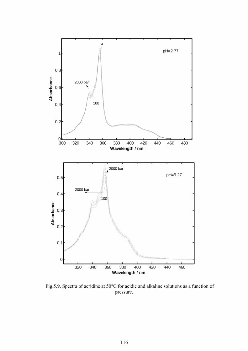
116
300 320 340 360 380 400 420 440 460 4800
0.2
0.4
0.6
0.8
1
Wavelength / nm
Abs
orba
nce
100
2000 bar
pH=2.77
320 340 360 380 400 420 440 460
0
0.1
0.2
0.3
0.4
0.5
Wavelength / nm
Abs
orba
nce
100
2000 bar
pH=9.27
2000 bar
Fig.5.9. Spectra of acridine at 50°C for acidic and alkaline solutions as a function of pressure.

117
Fig.5.10. Pressure and temperature dependence of ionisation constant of acridiniuim ion.

118
5.5. References
Albert A. and Goldacre R. (1946) Ionization of acridine bases. Journal of the Chemical Society, 706-13.
Boily J.-F. and Seward T. M. (2005) On the Dissociation of Methyl Orange: Spectrophotometric Investigation in Aqueous Solutions from 10 to 90 Deg and Theoretical Evidence for Intramolecular Dihydrogen Bonding. Journal of Solution Chemistry 34(12), 1387-1406.
Boily J.-F. and Suleimenov O. M. (2006) Extraction of Chemical Speciation and Molar Absorption Coefficients with Well-Posed Solutions of Beer's Law. Journal of Solution Chemistry 35(6), 917-926.
Bolton P. D., Ellis J., Fleming K. A., and Lantzke I. R. (1973) Protonation of azobenzene derivatives. I. Methyl orange and o-methyl orange. Australian Journal of Chemistry 26(5), 1005-14.
Bulemela E., Trevani L., and Tremaine P. R. (2005) Ionization Constants of Aqueous Glycolic Acid at Temperatures up to 250°C Using Hydrothermal pH Indicators and UV-Visible Spectroscopy. Journal of Solution Chemistry 34(7), 769-788.
Ellis A. J. (1963) The ionization, acetic, propionic, butyric, and benzoic acids in water, from conductance measurements up to 225 Deg. Journal of the Chemical Society, 2299-310.
Fernandez D. P., Goodwin A. R. H., Lemmon E. W., Sengers J. M. H. L., and Williams R. C. (1997) A formulation for the static permittivity of water and steam at temperatures from 238 K to 873 K at pressures up to 1200 MPa, including derivatives and Debye-Hueckel coefficients. Journal of Physical and Chemical Reference Data 26(4), 1125-1166.
Ho P. C. and Palmer D. A. (1996) Ion association of dilute aqueous sodium hydroxide solutions to 600 DegC and 300 MPa by conductance measurements. Journal of Solution Chemistry 25(8), 711-729.
Huh Y., Lee J. G., McPhail D. C., and Kim K. (1993) Measurement of pH at elevated temperatures using the optical indicator acridine. Journal of Solution Chemistry 22(7), 651-61.
Jia Z., Ramstad T., and Zhong M. (2001) Medium-throughput pKa screening of pharmaceuticals by pressure-assisted capillary electrophoresis. Electrophoresis 22(6), 1112-1118.
Kestin J., Sengers J. V., Kamgar-Parsi B., and Sengers J. M. H. L. (1984) Thermophysical properties of fluid water. Journal of Physical and Chemical Reference Data 13(1), 175-83.
Lee I.-J., Jung G.-S., and Kim K. (1994) Spectrophotometric determination of dissociation constants for propionic acid and 2,5-dinitrophenol at elevated temperatures. Journal of Solution Chemistry 23(12), 1283-92.
Lee J. G., Kim K., Cho B. R., and Kim S. J. (1992) A study on the oxidation of the pH indicator acridine in aqueous solution at elevated temperature. Journal of the Korean Chemical Society 36(3), 466-7.
Lown D. A., Thirsk H. R., and Wynne-Jones L. (1970) Temperature and pressure dependence of the volume of ionization of acetic acid in water from 25 to 225°C and 1 to 3000 bars. Transactions of the Faraday Society 66(1), 51-73.
Marshall W. L. and Franck E. U. (1981) Ion product of water substance, 0-1000°C, 1-10,000 bars, new international formulation and its background. Journal of Physical and Chemical Reference Data 10(2), 295-304.

119
Mesmer R. E., Patterson C. S., Busey R. H., and Holmes H. F. (1989) Ionization of acetic acid in aq. sodium chloride media: a potentiometric study to 573K and 130 bar. Journal of Physical Chemistry 93(21), 7483-90.
Pavlyuk L. A. and Smolyakov B. S. (1974a) Spectrophotometric determination of the ionization constant of bromphenol blue in the 25-150.deg. temperature interval. Izvestiya Sibirskogo Otdeleniya Akademii Nauk SSSR, Seriya Khimicheskikh Nauk(5), 22-4.
Pavlyuk L. A. and Smolyakov B. S. (1974b) Ionization constant of o- and p-nitrophenols at temperatures from 25 to 175.deg. Izvestiya Sibirskogo Otdeleniya Akademii Nauk SSSR, Seriya Khimicheskikh Nauk(5), 16-21.
Ros M. P., Thomas J., Crovetto G., and Llor J. (1998) Thermodynamics of proton dissociation of acridinium ion in aqueous solution. Reactive & Functional Polymers 36(3), 217-220.
Rosenberg L. S., Simons J., and Schulman S. G. (1979) Determination of pKa values of N-heterocyclic bases by fluorescence spectrophotometry. Talanta 26(9), 867-71.
Ryan E. T., Xiang T., Johnston K. P., and Fox M. A. (1997) Absorption and Fluorescence Studies of Acridine in Subcritical and Supercritical Water. Journal of Physical Chemistry A 101(10), 1827-1835.
Shock E. L. and Koretsky C. M. (1993) Metal-organic complexes in geochemical processes: calculation of standard partial molal thermodynamic properties of aqueous acetate complexes at high pressures and temperatures. Geochimica et Cosmochimica Acta 57(20), 4899-922.
Suleimenov O. M. and Seward T. M. (2000) Spectrophotometric measurements of metal complex formation at high temperatures: the stability of Mn(II) chloride species. Chemical Geology 167(1-2), 177-192.
Suleimenov O. M. (2004) Simple, compact, flow-through, high temperature high pressure cell for UV-Vis spectrophotometry. Review of Scientific Instruments 75(10, Pt. 1), 3363-3364.
Tsuda M., Shirotani I., Minomura S., and Terayama Y. (1976) The effect of pressure on the dissociation of weak acids in aqueous buffers. Bulletin of the Chemical Society of Japan 49(11), 2952-5.
Xiang T. and Johnston K. P. (1994) Acid-Base Behavior of Organic Compounds in Supercritical Water. Journal of Physical Chemistry 98(32), 7915-22.
Yamazaki H., Sperline R. P., and Freiser H. (1992) Spectrophotometric determination of pH and its application to determination of thermodynamic equilibrium constants. Analytical Chemistry 64(22), 2720-5.

120
5.6. Appendix Appendix 5.6.1. Initial composition of solutions (mol/kg) and their pH used for calculation
of temperature dependence of pK for acridinium ion ionisation at 25-200°C.
Acridine CH3COONa HCl CH3COOH NaOH pH
calcul. pH
meas.
sol1 4.767E-06 0 2.310E-02 6.846E-05 0 1.67 1.68
sol2 3.942E-06 0 1.361E-03 1.374E-04 0 2.88 2.88
sol3 4.641E-06 0 0 5.027E-03 0 3.54 3.54
sol4 3.444E-06 0 0 1.219E-03 0 3.86 3.89
sol5 3.515E-06 2.104E-04 0 5.469E-04 0 4.44 4.46
sol6 3.519E-06 2.075E-04 0 1.227E-04 0 5.03 5.06
sol7 3.412E-06 9.689E-04 0 1.190E-04 0 5.66 5.67
sol8 3.508E-06 6.018E-03 0 1.223E-04 0 6.42 6.39
sol9 3.383E-06 0 0 1.183E-04 2.106E-04 9.95 9.96
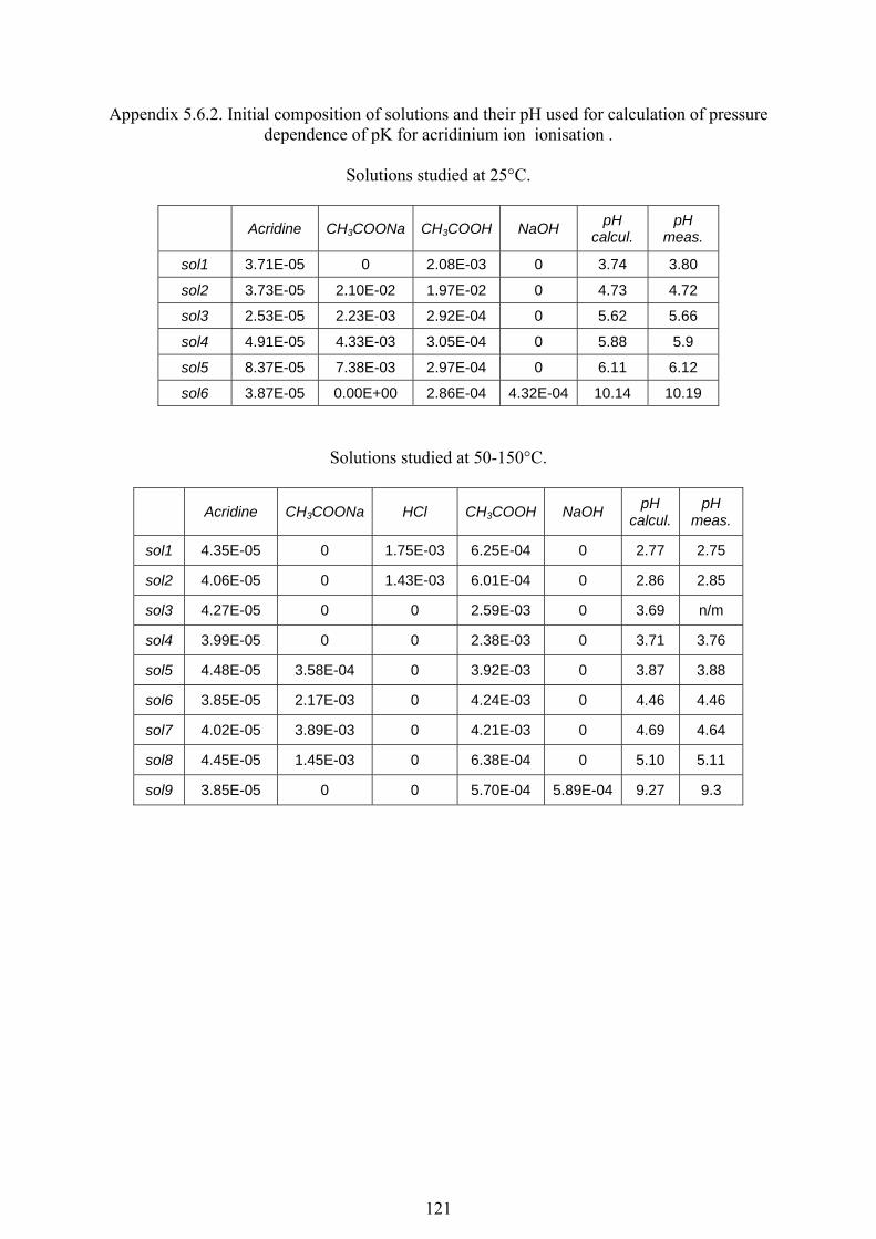
121
Appendix 5.6.2. Initial composition of solutions and their pH used for calculation of pressure dependence of pK for acridinium ion ionisation .
Solutions studied at 25°C.
Acridine CH3COONa CH3COOH NaOH pH calcul.
pH meas.
sol1 3.71E-05 0 2.08E-03 0 3.74 3.80
sol2 3.73E-05 2.10E-02 1.97E-02 0 4.73 4.72
sol3 2.53E-05 2.23E-03 2.92E-04 0 5.62 5.66
sol4 4.91E-05 4.33E-03 3.05E-04 0 5.88 5.9
sol5 8.37E-05 7.38E-03 2.97E-04 0 6.11 6.12
sol6 3.87E-05 0.00E+00 2.86E-04 4.32E-04 10.14 10.19
Solutions studied at 50-150°C.
Acridine CH3COONa HCl CH3COOH NaOH pH
calcul. pH
meas.
sol1 4.35E-05 0 1.75E-03 6.25E-04 0 2.77 2.75
sol2 4.06E-05 0 1.43E-03 6.01E-04 0 2.86 2.85
sol3 4.27E-05 0 0 2.59E-03 0 3.69 n/m
sol4 3.99E-05 0 0 2.38E-03 0 3.71 3.76
sol5 4.48E-05 3.58E-04 0 3.92E-03 0 3.87 3.88
sol6 3.85E-05 2.17E-03 0 4.24E-03 0 4.46 4.46
sol7 4.02E-05 3.89E-03 0 4.21E-03 0 4.69 4.64
sol8 4.45E-05 1.45E-03 0 6.38E-04 0 5.10 5.11
sol9 3.85E-05 0 0 5.70E-04 5.89E-04 9.27 9.3

122
6. Summary and Conclusions.
The aim of this thesis was to study the stability and stochiometry of aqueous
molybdate and tungstate species up to 300°C and at pressures close to equilibrium saturated
vapour pressure. Of particular interest were the protonation equilibria involving monomeric
molybdate and tungstate as a function of temperature and pH. The relevant equilibria, which
were studied, are ++↔ HHLLH -0
2 (6.1)
+−− +↔ HLHL 2 (6.2) ++ +↔ HLLH H 0
23 (6.3)
where H3L ,H2L, HL-, L2- correspond to H3MoO4+ , H2MoO4
0, HMoO4-,MoO4
2- and H3WO4+,
H2WO40, HWO4
-,WO42- according to the system considered.
The determination of the equilibrium constants and associated thermodynamic
parameters were facilitated by spectrophotometric measurements using a specially designed
high temperature optical cell employing quartz glass windows. Combined chemometric and
thermodynamic analysis of uv-vis spectrophotometric data were used to extract the
ionisation constants.
Coincidentally, the values of K1 and K2 for molybdic acid (reactions (6.1) and (6.2)
are almost identical at 25°C which has lead to much uncertainty in the previously published
values. In addition, essentially all previously studies were conducted at higher ionic strengths
and no reliable thermodynamic equilibrium constants were available at ambient temperature.
We therefore carried out extensive measurements to rectify this situation. The values of
logK0 = -1.02, logK1 = -4.12 and logK2 = -4.13 at 22°C represent the first reliable data at I=0.
At elevated temperatures, we have obtained the first experimentally based values
for the first and second ionisation (deprotonation) constants for molybdic acid up to 300°C.
The equations describing the temperature dependence of K1 and K2 from 25 to 300°C are
given by,
)ln(660.1702875.0125.96log 110 TTK ⋅+⋅−−= (6.4)
)ln(9366.502690.0082.30log 210 TTK ⋅+⋅−−= (6.5)

123
These new data represent a self-consistent set of thermodynamic constants which
permit the rigorous chemical modelling of molybdate transport and deposition by
hydrothermal fluids in the Earth’s crust up to 300°C and at moderate pressures.
We have also studied the stability of monomeric tungstate species up to 250°C. The
agreement of our data with few previously published reliable literature data for K1 and K2 at
25°C is excellent. At elevated temperatures, the only previous experimentally based data
result from the potentiometric study of Wesolowski et al. (1984). The agreement of our data
with theirs is only moderate with the discrepancy probably arising from the difficulties in the
data treatment of Wesolowski due to the presence of various polyanionic tungstate species as
well in our data treatment due to the position of the band maxima in the far uv region.
Finally, we note that the data presented in this thesis represent a first step towards a
more extensive understanding of hydrothermal molybdate and tungstate chemistry. An
important next step would be to build on this knowledge by extending our studies to the
formation of the thio-anions of both molybdate and tungstate (i.e.thiomolybdates and
thiotungstates) whose chemistry is essentially unknown at elevated temperatures and
pressures. This would give further important insight not only into Mo and W transport in ore
forming hydrothermal systems but also provide a basis with which to consider other
interesting aspects such as the temperature, redox and pH dependence of 97Mo/95Mo
fractionation in aqueous systems.
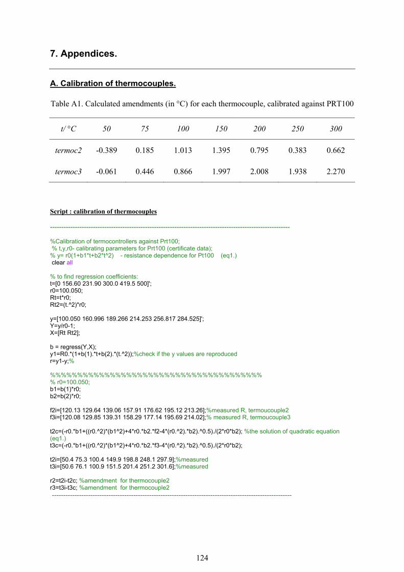
124
7. Appendices. A. Calibration of thermocouples. Table A1. Calculated amendments (in °C) for each thermocouple, calibrated against PRT100
t/ °C 50 75 100 150 200 250 300
termoc2 -0.389 0.185 1.013 1.395 0.795 0.383 0.662
termoc3 -0.061 0.446 0.866 1.997 2.008 1.938 2.270
Script : calibration of thermocouples ---------------------------------------------------------------------------------------------------------- %Calibration of termocontrollers against Prt100; % t,y,r0- calibrating parameters for Prt100 (certificate data); % y= r0(1+b1*t+b2*t^2) - resistance dependence for Pt100 (eq1.) clear all % to find regression coefficients: t=[0 156.60 231.90 300.0 419.5 500]'; r0=100.050; Rt=t*r0; Rt2=(t.^2)*r0; y=[100.050 160.996 189.266 214.253 256.817 284.525]'; Y=y/r0-1; X=[Rt Rt2]; b = regress(Y,X); y1=R0.*(1+b(1).*t+b(2).*(t.^2));%check if the y values are reproduced r=y1-y;% %%%%%%%%%%%%%%%%%%%%%%%%%%%%%%%%%%%%%%% % r0=100.050; b1=b(1)*r0; b2=b(2)*r0; f2i=[120.13 129.64 139.06 157.91 176.62 195.12 213.26];%measured R, termoucouple2 f3i=[120.08 129.85 139.31 158.29 177.14 195.69 214.02];% measured R, termoucouple3 t2c=(-r0.*b1+((r0.^2)*(b1^2)+4*r0.*b2.*f2-4*(r0.^2).*b2).^0.5)./(2*r0*b2); %the solution of quadratic equation (eq1.) t3c=(-r0.*b1+((r0.^2)*(b1^2)+4*r0.*b2.*f3-4*(r0.^2).*b2).^0.5)./(2*r0*b2); t2i=[50.4 75.3 100.4 149.9 198.8 248.1 297.9];%measured t3i=[50.6 76.1 100.9 151.5 201.4 251.2 301.6];%measured r2=t2i-t2c; %amendment for thermocouple2 r3=t3i-t3c; %amendment for thermocouple2 ----------------------------------------------------------------------------------------------------------

125
B. Determination of the cell’s path length In order to determine pathlength of the Ti-Pd cell, the same solution was analyzed in a 1cm cuvette and
in the cell at the same conditions (the same day). According to Beer’s law the ratio of the absorbance
values gives the ratio in pathlengths.
Script : determine pathlength of the cell
---------------------------------------------------------------------------------------------------------- %%%%%%%%%%%%spectra of solutions analyzed in 1cm cuvette %blank w_kuv1=csvread('w_kuv1.csv',2); w_kuv2=csvread('w_kuv2.csv',2); w_kuv3=csvread('w_kuv3.csv',2); w_kuv4=csvread('w_kuv4.csv',2); w_kuv5=csvread('w_kuv5.csv',2); w_kuv6=csvread('w_kuv6.csv',2); w_kuv7=csvread('w_kuv7.csv',2); w_kuv8=csvread('w_kuv8.csv',2); w_kuv9=csvread('w_26_kuv.csv',2); %solutions sol_kuv1=csvread('s_kuv1.csv',2); sol_kuv2=csvread('s_kuv2.csv',2); sol_kuv3=csvread('s_kuv3.csv',2); sol_kuv4=csvread('s_kuv4.csv',2); sol_kuv5=csvread('s_kuv5.csv',2); sol_kuv6=csvread('s_kuv6.csv',2); sol_kuv7=csvread('s_kuv7.csv',2); sol_kuv8=csvread('s_kuv8.csv',2); sol_kuv9=csvread('s_26_kuv.csv',2); Skuv=[sol_kuv2(:,2) sol_kuv3(:,2) sol_kuv4(:,2) sol_kuv5(:,2) sol_kuv6(:,2) sol_kuv7(:,2) sol_kuv8(:,2) sol_kuv9(:,2)]; Wkuv=[w_kuv1(:,2) w_kuv1(:,2) w_kuv1(:,2) w_kuv1(:,2) w_kuv1(:,2) w_kuv1(:,2) w_kuv1(:,2) w_kuv9(:,2)]; solkuv=Skuv-Wkuv;%spectra of solutions, corrected for background absorbance lambda=w_kuv1(:,1);%wavelength %plot spectra figure plot(lambda,solkuv) title('sol-blank/cuvette') %%%%%%%%%%spectra of solutions analyzed in Ti-Pd cell %blank w_cell=csvread('w_cell1.csv',2); w_cel2=csvread('w_27m_25.csv',2); w_cel3=csvread('w_30m_25.csv',2); w_cel4=csvread('w_2ju_25.csv',2); w_cel5=csvread('w_25m_25.csv',2); w_cel6=csvread('w_10ju_25.csv',2); w_cel7=csvread('w_15d_25b.csv',2); w_cel8=csvread('w_29n_25.csv',2); w_cel9=csvread('w_26f_25a.csv',2);% %solutions s_cell=csvread('s_cell1.csv',2);% s_cel2=csvread('s_27m_25.csv',2); s_cel3=csvread('s_30m_25.csv',2); s_cel4=csvread('s_2ju_25.csv',2); s_cel5=csvread('s_25m_25.csv',2); s_cel6=csvread('s_10ju_25.csv',2); s_cel7=csvread('s_15d_25.csv',2); s_cel8=csvread('s_29n_25.csv',2); s_cel9=csvread('sol_26f_cell.csv',2);% Scell=[ s_cel2(:,2) s_cel3(:,2) s_cel4(:,2) s_cel5(:,2) s_cel6(:,2) s_cel7(:,2) s_cel8(:,2) s_cel9(:,2)]; Wcell=[ w_cel2(:,2) w_cel3(:,2) w_cel4(:,2) w_cel5(:,2) w_cel6(:,2) w_cel7(:,2) w_cel8(:,2) w_cel9(:,2)]; solcell=Scell-Wcell;%spectra of solutions, corrected for background absorbance

126
%plot spectra figure plot(lambda,solcell) title('sol-blank/cell') %%%%%%%%%%%%%%%%%%%%%%%%%%%% [Amaxcuvn,Icuvn]= max(solkuv,[],1);% find max value of absorbance Amax and its index I %%cuvette [Amaxcelln,Icelln]= max(solcell,[],1);% find max value of absorbance Amax and its index I%%cell %or average for the interval: qn=solcell./solkuv;%ratio of maximum values=pathlength q=mean(qn);%average value ---------------------------------------------------------------------------------------------------------- C. Background Absorbance C1. Association / dissociation constants for the components of background absorbance.
1.6 1.8 2 2.2 2.4 2.6 2.8 3 3.2 3.4 3.6-2
-1.5
-1
-0.5
0
0.5
1
1.5
1000/T, 1/°C
logK
ass
Ho et al.,2000Ho et al.,1996Barns,1997Plyasunov et al.,1988Chen et al., 1992Bianchi et al., 1994Gimblet et al.,1954Simonin et al.,1998Robertis et al.,1984
Fig. C1.1. Previously reported values for the association constant of sodium hydrooxide.
0 50 100 150 200 2504.6
4.8
5
5.2
5.4
5.6
5.8
6
t/°C
logK
diss
Ellis,1963
Lown et al.,1970
Mesmer et al.,1989
Zotov et al.,2002
Fisheret al., 1972
Mellon et al., 1973
Fig. C1.2. Previously reported values for the dissociation constant of acetic acid.

127
C2. Densities for the components of background absorbance. C 2.1 .Script : Density of sodium perchlorate from molar concentr; ---------------------------------------------------------------------------------------------------------- function [dna]=dens_sodiumperchlor(mu) %density of NaClO4 %mu-molar concentration dna=0.99834+0.076913.*mu-0.00039159.*mu.^2; %janz,1969 % dna=0.9957+0.07919*mu-0.00185*mu^1.5; %miller,1956 %dna=0.9971+0.0768*mu; %Jones,1945 ---------------------------------------------------------------------------------------------------------- C 2.2.Script : Density of sodium perchlorate from molal concentr; ---------------------------------------------------------------------------------------------------------- function [rona]=dens_naperchlor(conc) %density of NaClO4 %conc-molal concentration Mm=122.45; %molar mass of NaClO4 %eq1: dna=0.99834+0.076913*mu-0.00039159*mu^2; %%%formula for the density of sodium perchlorate ; janz 1969(molar concentrations) %eq2: mu=conc*dna*1000/(conc*Mm+1000); %%%%%%folrmula of converting molal concentration 'conc' to molar concentration 'mu' %eq3: dna =.99834+76.913000*conc*dna/(conc*Mm+1000)-391.5900000*conc^2*dna^2/(conc*Mm +1000)^2; %%% result of substituting eq1 in eq2 %analytical solution of eq3 rona=.2553691361e-7./conc.^2.*(-.5000000000e11-50000.*conc.^2.*Mm.^2-100000000.*conc.*Mm+3845650.*conc.^2.*Mm+3845650000.*conc+10.*(-.3845650000e19.*conc+.1000000000e18.*conc.*Mm+.1500000000e15.*conc.^2.*Mm.^2-.1153695000e17.*conc.^2.*Mm+.1869842353e18.*conc.^2+.2500000000e20+25000000.*conc.^4.*Mm.^4+.1000000000e12.*conc.^3.*Mm.^3-3845650000.*conc.^4.*Mm.^3-.1153695000e14.*conc.^3.*Mm.^2+.1869842353e12.*conc.^4.*Mm.^2+.3739684706e15.*conc.^3.*Mm).^(1/2)); %rona2=.2553691361e-7/conc^2*(-.5000000000e11-50000.*conc^2*Mm^2-100000000.*conc*Mm+3845650.*conc^2*Mm+3845650000.*conc-10.*(-.3845650000e19*conc+.1000000000e18*conc*Mm+.1500000000e15*conc^2*Mm^2-.1153695000e17*conc^2*Mm+.1869842353e18*conc^2+.2500000000e20+25000000.*conc^4*Mm^4+.1000000000e12*conc^3*Mm^3-3845650000.*conc^4*Mm^3-.1153695000e14*conc^3*Mm^2+.1869842353e12*conc^4*Mm^2+.3739684706e15*conc^3*Mm)^(1/2)); %the root without physical meaning ----------------------------------------------------------------------------------------------------------
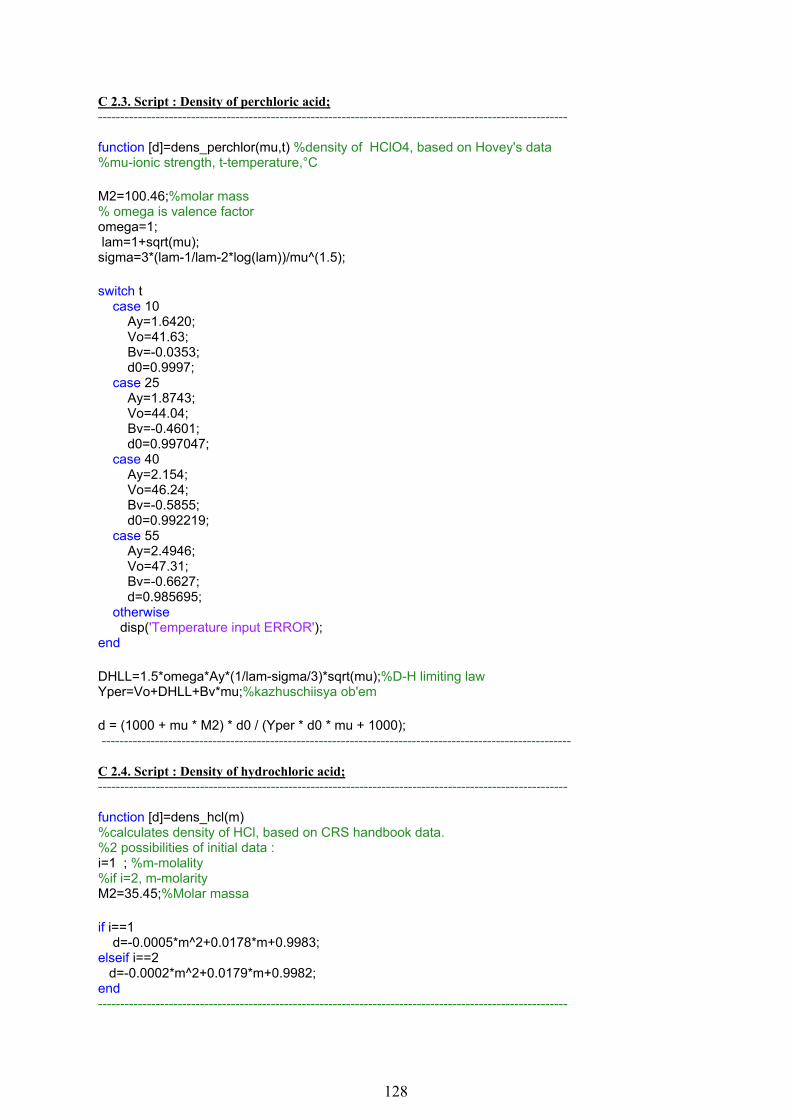
128
C 2.3. Script : Density of perchloric acid; ---------------------------------------------------------------------------------------------------------- function [d]=dens_perchlor(mu,t) %density of HClO4, based on Hovey's data %mu-ionic strength, t-temperature,°C M2=100.46;%molar mass % omega is valence factor omega=1; lam=1+sqrt(mu); sigma=3*(lam-1/lam-2*log(lam))/mu^(1.5); switch t case 10 Ay=1.6420; Vo=41.63; Bv=-0.0353; d0=0.9997; case 25 Ay=1.8743; Vo=44.04; Bv=-0.4601; d0=0.997047; case 40 Ay=2.154; Vo=46.24; Bv=-0.5855; d0=0.992219; case 55 Ay=2.4946; Vo=47.31; Bv=-0.6627; d=0.985695; otherwise disp('Temperature input ERROR'); end DHLL=1.5*omega*Ay*(1/lam-sigma/3)*sqrt(mu);%D-H limiting law Yper=Vo+DHLL+Bv*mu;%kazhuschiisya ob'em d = (1000 + mu * M2) * d0 / (Yper * d0 * mu + 1000); ---------------------------------------------------------------------------------------------------------- C 2.4. Script : Density of hydrochloric acid; ---------------------------------------------------------------------------------------------------------- function [d]=dens_hcl(m) %calculates density of HCl, based on CRS handbook data. %2 possibilities of initial data : i=1 ; %m-molality %if i=2, m-molarity M2=35.45;%Molar massa if i==1 d=-0.0005*m^2+0.0178*m+0.9983; elseif i==2 d=-0.0002*m^2+0.0179*m+0.9982; end ----------------------------------------------------------------------------------------------------------

129
C 2.5. Script : Density of sodium chloride; ---------------------------------------------------------------------------------------------------------- function [dnacl]=dens_sodiumchlor(m) %m-molality of NaCl %d0=0.997047;%density of water at 25C,Kestin 1984 d0=0.9970751;%density of water at 25°C, Kell,1967 M2=58.45;%molar mass of NaCl; %the equation taken from Potter,Brown,1977 A0=16.62; B0=1.773; C0=0.098; dnacl=(1000*d0+M2*m*d0)/(1000+A0*m*d0+B0*(m^1.5)*d0+C0*m^2*d0); C3. Influence of degassing procedure on water absorbance.
190 200 210 220 230 240 250
0.3
0.35
0.4
0.45
0.5
0.55
0.6
Abs
orba
nce
spectra
190 200 210 220 230 240 2500
0.02
0.04
0.06
Wavelength / nm
residuals
s1 - not degasseds2 - degasseds3 - degassed
Fig.C3.1 Spectra of pure water at 25°C. “s1” is not degassed water; “s2” is water which was degassed under partial vacuum in an ultrasonic bath periodically purged with oxygen-free argon; “s3” is the water purged of dissolved gases with an on-line vacuum degassing system (Alltech). Residuals represent the difference in absorbance between s1 and s2.

130
C4. Evidence of progressive dissolution of silica glass windows: gradual increase in blank water absorbance after several temperature cycles.
200 220 240 260 280 300 320 340-0.05
0
0.05
0.1
0.15
0.2
0.25
0.3
0.35
Wavelength / nm
Abs
orba
nce
1f3fa5f7f
Fig.C4.1. Spectra of pure water at 25°C taken before (1f) and after several temperature cycles 25-
300°C (3fa, 5f, 7f) .
200 220 240 260 280 300 320 340 360
0
0.01
0.02
0.03
0.04
0.05
0.06
0.07
0.08
Wavelength / nm
Abs
orba
nce
1s5s6s8f
Fig.C4.2. Spectra of pure water at 100°C taken before (1s) and after
several temperature cycles 25-200°C (5s,6s,8f) .
200 220 240 260 280 300 320 3400
0.02
0.04
0.06
0.08
0.1
0.12
0.14
0.16
Wavelength / nm
Abs
orba
nce
1f3f4f5f5s9s
Fig.C4.3.Spectra of pure water at 25°C taken before (1f) and after several temperature cycles 25-200°C (2f,3f,4f,5f) and after several temperature cycles 25-250°C (5s, 9s) .
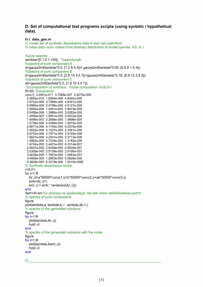
131
D. Set of computational test programs scripts (using syntetic / hypothetical data). D.1. data_gen.m % create set of synthetic Absorbance data to test calc-optimfunc % initial data -conc =taken from arbitrary distribution of model species h2l, hl, l %pure spectra lambda=[0.1:0.1:100]; %wavelength %spectra of pure component A a=gauss2mf(lambda*0.5, [1.2 8 5 4])+ gauss2mf(lambda*0.09, [0.8 8 1.5 4]); %spectra of pure component B b=gauss2mf(lambda*0.3, [2.8 15 4.5 7])+gauss2mf(lambda*0.18, [0.8 13 3.5 5]); %spectra of pure component C ab=gauss2mf(lambda*0.5, [1.8 15 4.5 7]); %Composition of solutions %total composition %h2l hl l R=20; %nsolutions conc=[ 3.0091e-011 3.7968e-007 4.9270e-005 2.3692e-010 1.0564e-006 4.8442e-005 2.9742e-009 3.7386e-006 4.8351e-005 6.6960e-009 5.4798e-006 4.6127e-005 2.9005e-008 1.0481e-005 3.8913e-005 5.5408e-008 1.3988e-005 3.6282e-005 1.2856e-007 1.9551e-005 3.0533e-005 7.4496e-007 3.2898e-005 1.4898e-005 1.2736e-006 4.4396e-005 1.5915e-005 2.8817e-006 4.1740e-005 6.2070e-006 3.3022e-006 4.1427e-005 5.3361e-006 5.0742e-006 3.7971e-005 2.9193e-006 7.6627e-006 4.2001e-005 2.3713e-006 1.0862e-005 3.7239e-005 1.3183e-006 1.4744e-005 3.4431e-005 8.3314e-007 2.0627e-005 2.8349e-005 4.0634e-007 2.5300e-005 2.5138e-005 2.6190e-007 3.0639e-005 1.7567e-005 1.0683e-007 3.4959e-005 1.2863e-005 5.0828e-008 4.4609e-005 6.3219e-006 1.0010e-008]'; % Synthetic absorbance matrix r=0.01; for i=1:R A(:,i)=a*50000*conc(1,i)+b*50000*conc(2,i)+ab*50000*conc(3,i); errb=A(:,i)*r; err(:,i) = errb.* rand(size(A(:,i))); end Aerr=A+err;%v principe ne ispolzuetsya, tak kak noise nakladibaetsya pozhe % spectra of pure components figure plot(lambda,a, lambda,b,'r', lambda,ab,'k') % spectra of the generated solutions figure for i=1:R plot(lambda,A(:,i)) hold all end % spectra of the generated solutions with the noise figure for i=1:R plot(lambda,Aerr(:,i)) hold all end %______________________________________________________________________

132
0 10 20 30 40 50 60 70 80 90 1000
0.1
0.2
0.3
0.4
0.5
0.6
0.7
0.8
Wavelength / nm
Abs
orba
nce
h2lhll
Fig. D1.1. Generated spectra of pure component.
0 10 20 30 40 50 60 70 80 90 1000
0.2
0.4
0.6
0.8
1
1.2
1.4
1.6
1.8
Wavelength / nm
Abs
orba
nce
Fig. D1.2. Generated spectra of the component “mix”.
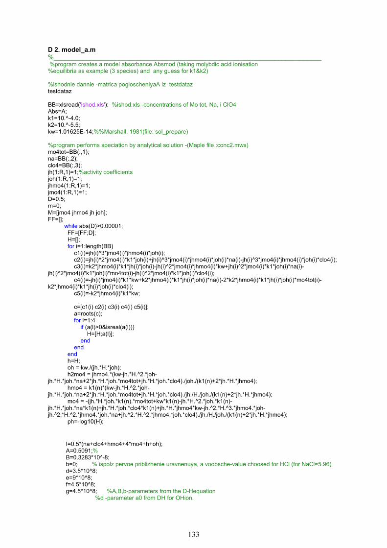
133
D 2. model_a.m %__________________________________________________________________________ %program creates a model absorbance Absmod (taking molybdic acid ionisation %equilibria as example (3 species) and any guess for k1&k2) %ishodnie dannie -matrica pogloscheniyaA iz testdataz testdataz BB=xlsread('ishod.xls'); %ishod.xls -concentrations of Mo tot, Na, i ClO4 Abs=A; k1=10.^-4.0; k2=10.^-5.5; kw=1.01625E-14;%%Marshall, 1981(file: sol_prepare) %program performs speciation by analytical solution -(Maple file :conc2.mws) mo4tot=BB(:,1); na=BB(:,2); clo4=BB(:,3); jh(1:R,1)=1;%activity coefficients joh(1:R,1)=1; jhmo4(1:R,1)=1; jmo4(1:R,1)=1; D=0.5; m=0; M=[jmo4 jhmo4 jh joh]; FF=[]; while abs(D)>0.00001; FF=[FF;D]; H=[]; for i=1:length(BB) c1(i)=jh(i)^3*jmo4(i)*jhmo4(i)*joh(i); c2(i)=jh(i)^2*jmo4(i)*k1*joh(i)+jh(i)^3*jmo4(i)*jhmo4(i)*joh(i)*na(i)-jh(i)^3*jmo4(i)*jhmo4(i)*joh(i)*clo4(i); c3(i)=k2*jhmo4(i)*k1*jh(i)*joh(i)-jh(i)^2*jmo4(i)*jhmo4(i)*kw+jh(i)^2*jmo4(i)*k1*joh(i)*na(i)-jh(i)^2*jmo4(i)*k1*joh(i)*mo4tot(i)-jh(i)^2*jmo4(i)*k1*joh(i)*clo4(i); c4(i)=-jh(i)*jmo4(i)*k1*kw+k2*jhmo4(i)*k1*jh(i)*joh(i)*na(i)-2*k2*jhmo4(i)*k1*jh(i)*joh(i)*mo4tot(i)-k2*jhmo4(i)*k1*jh(i)*joh(i)*clo4(i); c5(i)=-k2*jhmo4(i)*k1*kw; c=[c1(i) c2(i) c3(i) c4(i) c5(i)]; a=roots(c); for l=1:4 if (a(l)>0&isreal(a(l))) H=[H;a(l)]; end end end h=H; oh = kw./(jh.*H.*joh); h2mo4 = jhmo4.*(kw-jh.*H.^2.*joh-jh.*H.*joh.*na+2*jh.*H.*joh.*mo4tot+jh.*H.*joh.*clo4)./joh./(k1(n)+2*jh.*H.*jhmo4); hmo4 = k1(n)*(kw-jh.*H.^2.*joh-jh.*H.*joh.*na+2*jh.*H.*joh.*mo4tot+jh.*H.*joh.*clo4)./jh./H./joh./(k1(n)+2*jh.*H.*jhmo4); mo4 = -(jh.*H.*joh.*k1(n).*mo4tot+kw*k1(n)-jh.*H.^2.*joh.*k1(n)-jh.*H.*joh.*na*k1(n)+jh.*H.*joh.*clo4*k1(n)+jh.*H.*jhmo4*kw-jh.^2.*H.^3.*jhmo4.*joh-jh.^2.*H.^2.*jhmo4.*joh.*na+jh.^2.*H.^2.*jhmo4.*joh.*clo4)./jh./H./joh./(k1(n)+2*jh.*H.*jhmo4); ph=-log10(H); I=0.5*(na+clo4+hmo4+4*mo4+h+oh); A=0.5091;% B=0.3283*10^-8; b=0; % ispolz pervoe priblizhenie uravnenuya, a voobsche-value choosed for HCl (for NaCl=5.96) d=3.5*10^8; e=9*10^8; f=4.5*10^8; g=4.5*10^8; %A,B,b-parameters from the D-Hequation %d -parameter a0 from DH for OHion,

134
%e -parameter a0 from DH for Hion, %f-parameter a0 from DH for hmo4 ion, %g-parameter a0 from DH for mo4 ion logjmo4=-(A*4*I.^0.5)./(1+B*g*I.^0.5)+b*I; logjhmo4=-(A*1*I.^0.5)./(1+B*f*I.^0.5)+b*I; logjh=-(A*1*I.^0.5)./(1+B*e*I.^0.5)+b*I; logjoh=-(A*1*I.^0.5)./(1+B*d*I.^0.5)+b*I; jmo4c=10.^(logjmo4); jhmo4c=10.^(logjhmo4); jhc=10.^(logjh); johc=10.^(logjoh); D=jh-jhc; jh=jhc; jmo4=jmo4c; jhmo4=jhmo4c; joh=johc; m=m+1; M=[M;jmo4c jhmo4c jhc johc]; end conc=[h2mo4 hmo4 mo4 h oh]; %matrix of calculated molal concentrations H2MoO4,HMoO4,MoO4,H,OH for i=1:R Mm(i,:)=[205.95 204.95 203.45 1 17 ];;%matrix of molar masses H3MoO4,H2MoO4,HMoO4,MoO4,H,OH end data=conc*dw*1000./(conc.*Mm+1000);%calculate molar concentr ph=-log10(data(:,4)); dat=data(:,1:3); %minimize difference between absorbance matr [u,s,v]=svds(Abs,3); r=dat'/v'; cmod=(r*v')';% cmod=(inv(r)\v')'; %from help:One way to solve Ax=b is with x = inv(A)*b. A better way, % from both an execution time and numerical accuracy standpoint, %is to use the matrix division operator x = A\b.%%This produces the solution %using Gaussian elimination, without forming the inverse. %for details :see help mldivide\,mrdivide/ eps=u*s/r;% eps=u*s*inv(r) (pochti ravnoznachno) Absmod=eps*dat'; Absred=u*s*v'; %F=(cmod-dat)./dat; F=Absmod-Absred; figure plot(lambda,Abs) title('Absorbance') figure plot(lambda,eps) title('molar ext coef') figure plot(ph,dat) title('distrib diagram') %__________________________________________________________________________

135
D3. calc6a.m %__________________________________________________________________________ %programm optimizes konstants x0 using minimization of Absmod-Absred %belong to a group of testing programms. %input data: Absa.xls- model absorbance matrix A , created in model_a.m %with implied K1=-4.5 k2=-5.5 format short e A=xlsread('Absa.xls'); %add noise to model absorbance matrix r=0.01; for i=1:20 errb=A(:,i)*r; err(:,i) = errb.* rand(size(A(:,i))); end Abs=A+err; lambda=[0.1:0.1:100]; % x0=[-4.3 -4.9];%initial guess options=optimset('Display','iter','TolX',1e-4,'LevenbergMarquardt','on','MaxFunEvals',200,'TolFun',1e-5); x=lsqnonlin(@optimfunc6a,x0,[],[],options,Abs,lambda); [F,eps,Absmod,Ared]=optimfunc6a(x,Abs,lambda); Absmod=F+Ared; figure plot(lambda,Abs) figure plot(lambda,eps) figure plot(lambda,Absmod,'b',lambda,Ared,'r') figure plot(lambda,Absmod,'b',lambda,A,'r') function[F,eps,Absmod,Ared]=optimfunc6a(x,Abs,lambda) R=20; BB=xlsread('ishoda.xls'); k1=10.^x(1); k2=10.^x(2); kw=1.01625E-14;%%Marshall, 1981(file sol_prepare) %__________________________________________________________________________

136
D4. optimfunc6a.m %__________________________________________________________________________ % %program performs speciation by analytical solution -(maple file :conc2.mws) mo4tot=BB(:,1); na=BB(:,2); clo4=BB(:,3); jh(1:R,1)=1;%activity coefficients joh(1:R,1)=1; jhmo4(1:R,1)=1; jmo4(1:R,1)=1; D=0.5; M=[jmo4 jhmo4 jh joh]; FF=[]; while abs(D)>0.00001; FF=[FF;D]; H=[]; for i=1:length(BB) c=[c1(i,n,nn) c2(i,n,nn) c3(i,n,nn) c4(i,n,nn) c5(i,n,nn)]; c2(i)=jh(i)^2*jmo4(i)*k1*joh(i)+jh(i)^3*jmo4(i)*jhmo4(i)*joh(i)*na(i)-jh(i)^3*jmo4(i)*jhmo4(i)*joh(i)*clo4(i); c3(i)=k2*jhmo4(i)*k1*jh(i)*joh(i)-jh(i)^2*jmo4(i)*jhmo4(i)*kw+jh(i)^2*jmo4(i)*k1*joh(i)*na(i)-jh(i)^2*jmo4(i)*k1*joh(i)*mo4tot(i)-jh(i)^2*jmo4(i)*k1*joh(i)*clo4(i); c4(i)=-jh(i)*jmo4(i)*k1*kw+k2*jhmo4(i)*k1*jh(i)*joh(i)*na(i)-2*k2*jhmo4(i)*k1*jh(i)*joh(i)*mo4tot(i)-k2*jhmo4(i)*k1*jh(i)*joh(i)*clo4(i); c5(i)=-k2*jhmo4(i)*k1*kw; a=roots(c); for l=1:4 if (a(l)>0&isreal(a(l))) H=[H;a(l)]; end end end h=H; oh = kw./(jh.*H.*joh); h2mo4 = jhmo4.*(kw-jh.*H.^2.*joh-jh.*H.*joh.*na+2*jh.*H.*joh.*mo4tot+jh.*H.*joh.*clo4)./joh./(k1(n)+2*jh.*H.*jhmo4); hmo4 = k1(n)*(kw-jh.*H.^2.*joh-jh.*H.*joh.*na+2*jh.*H.*joh.*mo4tot+jh.*H.*joh.*clo4)./jh./H./joh./(k1(n)+2*jh.*H.*jhmo4); mo4 = -(jh.*H.*joh.*k1(n).*mo4tot+kw*k1(n)-jh.*H.^2.*joh.*k1(n)-jh.*H.*joh.*na*k1(n)+jh.*H.*joh.*clo4*k1(n)+jh.*H.*jhmo4*kw-jh.^2.*H.^3.*jhmo4.*joh-jh.^2.*H.^2.*jhmo4.*joh.*na+jh.^2.*H.^2.*jhmo4.*joh.*clo4)./jh./H./joh./(k1(n)+2*jh.*H.*jhmo4); ph=-log10(H); I=0.5*(na+clo4+hmo4+4*mo4+h+oh); A=0.5091;% B=0.3283*10^-8;% b=0; % ispolz pervoe priblizhenie uravnenuya, a voobsche-value choosed for HCl (for NaCl=5.96) d=3.5*10^8; e=9*10^8; f=4.5*10^8; g=4.5*10^8; %A,B,b-parameters from the D-Hequation %d -parameter a0 from DH for OHion, %e -parameter a0 from DH for Hion, %f-parameter a0 from DH for hmo4 ion, %g-parameter a0 from DH for mo4 ion logjmo4=-(A*4*I.^0.5)./(1+B*g*I.^0.5)+b*I; logjhmo4=-(A*1*I.^0.5)./(1+B*f*I.^0.5)+b*I; logjh=-(A*1*I.^0.5)./(1+B*e*I.^0.5)+b*I; logjoh=-(A*1*I.^0.5)./(1+B*d*I.^0.5)+b*I; jmo4c=10.^(logjmo4); jhmo4c=10.^(logjhmo4);

137
jhc=10.^(logjh); johc=10.^(logjoh); D=jh-jhc; jh=jhc; jmo4=jmo4c; jhmo4=jhmo4c; joh=johc; M=[M;jmo4c jhmo4c jhc johc]; end conc=[h2mo4 hmo4 mo4 h oh]; %matrix of calculated molal concentrations H2MoO4,HMoO4,MoO4,H,OH for i=1:R Mm(i,:)=[205.95 204.95 203.45 1 17 ];;%matrix of molar masses H2MoO4,HMoO4,MoO4,H,OH end data=conc*dw*1000./(conc.*Mm+1000);%calculate molar concentr ph=-log10(data(:,4)); dat=data(:,1:3); [u,s,v]=svds(Abs,3);%minimize difference between absorbance matr t=u*s; r=dat'/v'; eps=t/r;% Absmod=eps*dat'; Ared=u*s*v';%reduced matrix F=(Absmod-Ared);% %objectice function %__________________________________________________________________________

138
E. Set of computational program scripts, used for calculation / optimization of the equilibrium constants from uv spectrophotometric data (using molybdic acid as an example). E.1. Script “calc_ac”, optimizing objective function ---------------------------------------------------------------------------------------------------------- %programm optimizes konstants x0 clear all %import data data_ext %extract experimental data (spectra, corrected to blank absorbance) format short e [u,s,v]=svds(Absorb,4);%svd-decomposition of Absorb matrix x0=[-1.0 -4.0 -4.5];%initial guess for konstants %optimization parameters options = optimset('Display','iter','TolX',1e-6,'LevenbergMarquardt','on','MaxFunEvals',200,'TolFun',1e-5); x=lsqnonlin(@optimfunc6_h3l,x0,[],[],options,BB,R,u,s,v,dna); [F,epsil,Absmod,Absred,ph,data]=optimfunc6_h3l(x,BB,R,u,s,v,dna); %grafs: %plot ext. coeff. figure hplot=(lambda,epsil) title('epsilon') set(hplot,'LineWidth',1.5) set(gcf,'Color',[1 1 1]) xlabel(‘Wavelength / nm’) ylabel('Molar absrptivity’) %plot model and experimental absorbances with their residuals figure subplot(2,1,1), plot(lambda,Absmod,'b',lambda,Absorb,'r') title('Absmod-b/Absorb-r') subplot(2,1,2),plot(lambda,Absmod-Absorb) title('residuals') %plot species distribution diagram figure hplot1=plot(ph,dat) title('distribution diagram') set(hplot1,'LineWidth',1.5) set(gcf,'Color',[1 1 1]) xlabel(‘pH’) ylabel('Mo tot') %display calculated constants x ----------------------------------------------------------------------------------------------------------

139
E.2. Script “calc_ac”, speciation model, finding the objective function, ---------------------------------------------------------------------------------------------------------- function [F,epsil,Absmod,Absred,ph,data]=optimfunc6_h3l(x,BB,R,u,s,v,dna) %no iterative procedure to calcute activity coefficients, => apparent %equilibrium constants k1=10.^x(2); k2=10.^x(3); k3=10.^x(1); kw=1.4686e-014;%dissociation constant at 25°C, Marshall 1981 %program performs speciation by analytical solution -(maple file :conc_h3l) mo4tot=BB(:,1); na=BB(:,2); clo4=BB(:,3); jh(1:R,1)=1;%activity coefficients joh(1:R,1)=1; jhmo4(1:R,1)=1; jh3mo4(1:R,1)=1; jmo4(1:R,1)=1; kor=[]; for i=1:length(BB) c1(i)=jh(i)^4*jmo4(i)*jhmo4(i)*joh(i); c2(i)=k3*jh3mo4(i)*jh(i)^3*jmo4(i)*jhmo4(i)*joh(i)+jh(i)^4*jmo4(i)*jhmo4(i)*joh(i)*na(i)-jh(i)^4*jmo4(i)*jhmo4(i)*joh(i)*clo4(i)+jh(i)^4*jmo4(i)*jhmo4(i)*joh(i)*mo4tot(i); c3(i)=-jh(i)^3*jmo4(i)*jhmo4(i)*kw+k3*jh3mo4(i)*jh(i)^3*jmo4(i)*jhmo4(i)*joh(i)*na(i)-k3*jh3mo4(i)*jh(i)^3*jmo4(i)*jhmo4(i)*joh(i)*clo4(i)+k3*jh3mo4(i)*k1*jh(i)^2*jmo4(i)*joh(i); c4(i)=k3*jh3mo4(i)*k1*jh(i)^2*jmo4(i)*joh(i)*na(i)+k3*jh3mo4(i)*k1*k2*jhmo4(i)*jh(i)*joh(i)-k3*jh3mo4(i)*k1*jh(i)^2*jmo4(i)*joh(i)*clo4(i)-k3*jh3mo4(i)*k1*jh(i)^2*jmo4(i)*joh(i)*mo4tot(i)-k3*jh3mo4(i)*jh(i)^2*jmo4(i)*jhmo4(i)*kw; c5(i)=-k3*jh3mo4(i)*k1*jh(i)*jmo4(i)*kw+k3*jh3mo4(i)*k1*k2*jhmo4(i)*jh(i)*joh(i)*na(i)-k3*jh3mo4(i)*k1*k2*jhmo4(i)*jh(i)*joh(i)*clo4(i)-2*k3*jh3mo4(i)*k1*k2*jhmo4(i)*jh(i)*joh(i)*mo4tot(i); c6(i)=-k3*jh3mo4(i)*k1*k2*jhmo4(i)*kw; c=[c1(i) c2(i) c3(i) c4(i) c5(i) c6(i)]; b=roots(c); for l=1:5 if (b(l)>0&isreal(b(l))) kor=[kor;b(l)] ; end end end H=kor; h3mo4 = (2.*k2.*jhmo4.*k1.*jh.*H.*joh.*mo4tot+k2.*jhmo4.*k1.*kw-k2.*jhmo4.*k1.*jh.*H.^2.*joh-k2.*jhmo4.*k1.*jh.*H.*joh.*na+k2.*jhmo4.*k1.*jh.*H.*joh.*clo4+jh.^2.*H.^2.*jmo4.*k1.*joh.*mo4tot+jh.*H.*jmo4.*k1.*kw-jh.^2.*H.^3.*jmo4.*k1.*joh-jh.^2.*H.^2.*jmo4.*k1.*joh.*na+jh.^2.*H.^2.*jmo4.*k1.*joh.*clo4+jh.^2.*H.^2.*jmo4.*jhmo4.*kw-jh.^3.*H.^4.*jmo4.*jhmo4.*joh-jh.^3.*H.^3.*jmo4.*jhmo4.*joh.*na+jh.^3.*H.^3.*jmo4.*jhmo4.*joh.*clo4)./jh./H./joh./(2.*jh.*H.*jmo4.*k1+3.*k2.*jhmo4.*k1+jh.^2.*H.^2.*jmo4.*jhmo4); h = H; mo4 = -k2.*jhmo4.*k1.*(-jh.*H.*joh.*mo4tot-jh.*H.^2.*joh-jh.*H.*joh.*na+jh.*H.*joh.*clo4+kw)./jh./H./joh./(2.*jh.*H.*jmo4.*k1+3.*k2.*jhmo4.*k1+jh.^2.*H.^2.*jmo4.*jhmo4); oh = kw./jh./H./joh; hmo4 = -jmo4.*k1.*(-jh.*H.*joh.*mo4tot-jh.*H.^2.*joh-jh.*H.*joh.*na+jh.*H.*joh.*clo4+kw)./joh./(2.*jh.*H.*jmo4.*k1+3.*k2.*jhmo4.*k1+jh.^2.*H.^2.*jmo4.*jhmo4); h2mo4 = -jh.*H.*jmo4.*jhmo4.*(-jh.*H.*joh.*mo4tot-jh.*H.^2.*joh-jh.*H.*joh.*na+jh.*H.*joh.*clo4+kw)./joh./(2.*jh.*H.*jmo4.*k1+3.*k2.*jhmo4.*k1+jh.^2.*H.^2.*jmo4.*jhmo4); conc=[h3mo4 h2mo4 hmo4 mo4 h oh BB(:,4)];%matrix of calclulated molal concentrations H3MoO4,H2MoO4,HMoO4,MoO4,H,OH,NaClO4,

140
for i=1:R Mm(i,:)=[206.95 205.95 204.95 203.45 1 17 122.45];;%matrix of molar masses H3MoO4,H2MoO4,HMoO4,MoO4,H,OH,NaClO4
end data=conc*dna*1000./(conc.*Mm+1000);%calculate molar concentr ph=-log10(data(:,5)); dat=data(:,1:4); t=u*s; r=dat'/v';%rotation matrix epsil=t/r;% or epsil=t*inv(r) % epsil(find(epsil<0))=0;%filter for the negative epsilon Absmod=epsil*dat'; Absred=u*s*v';%reduced matrix %**** objective function F=(Absmod-Absred);% objective function ----------------------------------------------------------------------------------------------------------------------------

141
Aknowledgements.
First of all I would like to thank my supervisor Terry Seward, who made my come
to Zurich and PhD possible together with Diane Seward, who made me feel home upon my
arrival here.
I am very grateful to our group members: Oleg Suleimenov, Jean-Francois Boily
and Boris Taguirov for their invaluable help in the lab and useful advices at different stages
of my work.
I would like to thank Alex Teague, my group- and permanent officemate for the
last 4.5 years (congratulations, dude, you survived!)
Thank you, Katja, for joining our group. I enjoyed your company in our office and
appreciated your great support and friendship.
Furthemore, I wish to thank the following people for sharing lots of good and funny
moments:
-The Italian mafia: Chiara, Luca, Claudio, Sonia, Andrea, Fabio and Paola,
-The French and partly French community: Adélie, Leo, Pauline, Pierre and Marion,
-The numerous Russian (or, to be more precise, russian-speaking from former soviet
brotherhood) friends and colleagues from different departments of ETH, as well as from
outside (прошу прощения за такое безличное спасибо, постараюсь исправиться при
личной встрече),
-Colleagues and usual participants of Friday beer in the interval 2003-2007.
I am very grateful to my family for giving me support to all my initiatives since my
childhood, as well as Seb’s family for their almost daily (especially by the end) “Bon
courage” phrase.
And finally, thank you, Sebastien, for your inestimable patience and support
throughout my work on this thesis and for being (or sometimes not being ) there.

142
CURRICULUM VITAE
Zarina Minubayeva
Date of birth: 04 July, 1980
Citizenship: Russian Federation
Education:
1986-1990: Primary school. Tashkent, Uzbekistan
1990-1997: Secondary and high school. Moscow, Russian Federation
(With honours, “Silver medal”)
1997-2001: B.Sc. Environmental Geology, spec. Environmental Geochemistry.
Moscow State (Lomonosov) University (with honours) Thesis: “Hydrochemical features of the river drain and the influence of organic
matter on the migration forms of the elements (Using Klyazma river as an
illustration)”
2001-2002: Diploma (M.Sc.) Environmental Geology, spec. in Environmental
Geochemistry. Moscow State (Lomonosov) University (with honours) Thesis: “Experimental study of migration and aspects of environmental
geochemistry of mercury”
2002-present: Doctoral studies at the Institute of Mineralogy und Petrography,
Department of Earth Sciences, ETH Zürich, Switzerland