rights / license: research collection in copyright - non ...28471/...diss. eth no. 16173 assessing...
TRANSCRIPT

Research Collection
Doctoral Thesis
Assessing the carbon and water vapor fluxes in a temperategrassland using 13CO2 and H218O as system tracers
Author(s): Theis, Daniel Ethan
Publication Date: 2005
Permanent Link: https://doi.org/10.3929/ethz-a-005141264
Rights / License: In Copyright - Non-Commercial Use Permitted
This page was generated automatically upon download from the ETH Zurich Research Collection. For moreinformation please consult the Terms of use.
ETH Library

Diss. ETH No. 16173
Assessing the carbon and water vapor fluxes in a temperate
grassland using 13CO2 and H218O as system tracers
A dissertation submitted to the
SWISS FEDERAL INSTITUTE OF TECHNOLOGY ZURICH
for the degree of
DOCTOR OF SCIENCES
presented by
Daniel Ethan Theis
dipl. microbiol., University of Zurich
born 29th August 1972
citizen of Winterthur (ZH) and Schaffhausen (SH)
accepted on the recommendation of
Prof. Dr. Emmanuel Frossard, examiner
Prof. Dr. Hans Schnyder, TU Munich, co-examiner
Dr. Rolf Siegwolf, PSI Villigen, co-examiner
2005

II
Table of contents
Summary…………………………………………………………………………………………………………..V
Zusammenfassung………………………………………………………………………………………………VIII
1 General introduction...................................................................................................................................... 1
1.1 Rising atmospheric CO2 and the global carbon cycle .......................................................................... 1
1.2 Grassland ............................................................................................................................................. 2
1.2.1 Grassland soils............................................................................................................................ 2
1.2.2 The FACE experiment................................................................................................................ 3
1.3 Ecosystem-scale studies using stable isotopes ..................................................................................... 4
1.4 Objectives of this study........................................................................................................................ 5
2 A portable automated system for trace gas sampling in the field and stable isotope analysis in the
laboratory ................................................................................................................................................................ 6
2.1 Summary.............................................................................................................................................. 7
2.2 Introduction.......................................................................................................................................... 8
2.3 System design ...................................................................................................................................... 9
2.3.1 Overview .................................................................................................................................... 9
2.3.2 Operation.................................................................................................................................. 10
2.3.3 Computer control...................................................................................................................... 11
2.3.3.1 Sampling.............................................................................................................................. 11
2.3.3.2 Analysis ............................................................................................................................... 12
2.4 System performance........................................................................................................................... 13
2.4.1 Calibration of the Mass Spectrometer ...................................................................................... 13
2.4.2 Laboratory performance ........................................................................................................... 14
2.4.2.1 Storage effects ..................................................................................................................... 16
2.4.2.2 Automated compared to manual gas sampling and analysis................................................ 17
2.4.2.3 CO and CH4 isotope analysis............................................................................................... 18
2.4.3 Field performance..................................................................................................................... 20
2.5 Conclusions........................................................................................................................................ 21
2.6 Acknowledgements............................................................................................................................ 21
3 Dynamics of soil organic matter turnover and soil respired CO2 in a temperate grassland
labelled with carbon-13............................................................................................................................... 22
3.1 Summary............................................................................................................................................ 23
3.2 Introduction........................................................................................................................................ 24
3.3 Materials and methods ....................................................................................................................... 26
3.3.1 Experimental site ...................................................................................................................... 26
3.3.2 Sampling and analysis .............................................................................................................. 27
3.3.2.1 Bulk Soil .............................................................................................................................. 27
3.3.2.2 Soil air ................................................................................................................................. 28
III 3.3.2.3 Plant tissue........................................................................................................................... 29
3.3.2.4 Calculation of remaining labelled carbon ............................................................................ 29
3.3.2.5 Calculation of rhizosphere respiration ................................................................................. 30
3.3.2.6 Statistical analysis................................................................................................................ 30
3.4 Results................................................................................................................................................ 30
3.4.1 Plant material............................................................................................................................ 30
3.4.2 Soil organic matter (SOM) ....................................................................................................... 31
3.4.3 Calculation of new carbon after fumigation ............................................................................. 35
3.4.4 Soil respired CO2...................................................................................................................... 36
3.5 Discussion.......................................................................................................................................... 38
3.5.1 SOM carbon content and isotopic disequilibrium .................................................................... 38
3.5.2 Soil carbon exchange after fumigation ..................................................................................... 38
3.5.3 Effects of the dry summer 2003 on SOM and soil respiration ................................................. 39
3.5.4 Soil respired CO2...................................................................................................................... 40
3.6 Conclusions........................................................................................................................................ 41
3.7 Acknowledgements............................................................................................................................ 42
4 Partitioning of CO2 and H2O-vapor fluxes in a temperate grassland using stable isotopes ......................... 43
4.1 Summary............................................................................................................................................ 44
4.2 Introduction........................................................................................................................................ 46
4.3 Materials and Methods....................................................................................................................... 47
4.3.1 Experimental site ...................................................................................................................... 47
4.3.2 Sampling and analysis .............................................................................................................. 48
4.3.2.1 Net ecosystem exchange (NEE) .......................................................................................... 48
4.3.2.2 Air samples .......................................................................................................................... 49
4.3.2.3 Water vapor ......................................................................................................................... 49
4.3.2.4 Soil water............................................................................................................................. 50
4.3.2.5 Plant water and carbon......................................................................................................... 50
4.3.2.6 Meteorological data ............................................................................................................. 51
4.3.3 Calculations .............................................................................................................................. 51
4.3.3.1 Partitioning of CO2 fluxes.................................................................................................... 51
4.3.3.2 Partitioning of water vapor into evaporation and transpiration............................................ 53
4.3.3.3 Calculating canopy discrimination ...................................................................................... 55
4.3.4 Statistical analysis .................................................................................................................... 58
4.4 Results................................................................................................................................................ 58
4.4.1 NEE and micrometeorology ..................................................................................................... 58
4.4.2 Water vapor flux partitioning ................................................................................................... 60
4.4.3 Canopy discrimination.............................................................................................................. 62
4.4.3.1 Influence of transpiration on canopy discrimination ........................................................... 65
4.4.4 CO2 flux partitioning ............................................................................................................... 67
IV 4.4.4.1 Day – night course of CO2 and δ13C .................................................................................... 67
4.4.4.2 Keeling plots........................................................................................................................ 68
4.4.4.3 Assessment of CO2 fluxes FR and FA................................................................................... 72
4.5 Discussion.......................................................................................................................................... 77
4.5.1 Water vapor flux partitioning ................................................................................................... 77
4.5.1.1 Keeling plots of H2O ........................................................................................................... 78
4.5.2 Discrimination .......................................................................................................................... 78
4.5.3 Diurnal and inter-diurnal variations of Keeling plot intercepts ................................................ 80
4.5.4 CO2 flux partitioning ................................................................................................................ 82
4.5.5 Sensitivity analysis ................................................................................................................... 83
4.5.5.1 Calculation of ∆canopy............................................................................................................ 83
4.5.5.2 Calculation of FR and FA...................................................................................................... 83
4.5.6 Pooling of data.......................................................................................................................... 85
4.5.6.1 Pooling of different (former) CO2 treatments from FACE .................................................. 85
4.5.6.2 Pooling of different nitrogen fertilization levels.................................................................. 86
4.6 Conclusions........................................................................................................................................ 86
4.7 Acknowledgements............................................................................................................................ 87
5 General Discussion...................................................................................................................................... 88
5.1 A novel tool for air sampling ............................................................................................................. 88
5.2 CO2 and H2O flux partitioning........................................................................................................... 89
5.3 Carbon sequestration.......................................................................................................................... 90
5.4 13C as a system tracer ......................................................................................................................... 91
5.5 Outlook .............................................................................................................................................. 91
6 References ................................................................................................................................................... 93
Appendix – A short introduction to stable isotopes and their applications:………………………………………99
Acknowledgements…………..……………………………………………………………………………….....102
Curriculum vitae….………………………………………………………………...…...……...………………..103

V
Summary
In a managed temperate grassland site in Switzerland (Eschikon, ZH, 550 m a.s.l.), formerly
under ten years of “free air carbon dioxide enrichment” (FACE), a series of experiments was
conducted to investigate carbon fluxes and pools within this ecosystem. The study was carried
out for better quantifying the gross fluxes that are not fully understood at present. This is a
serious constraint towards the development of reliable models for estimating the impact of
future climate change and of rising CO2 concentrations.
A new approach to partition the net flux of CO2 (NEE) into assimilation (FA) and respiratory
fluxes (FR) using 13CO2 and H218O was tested. Discrimination of the plant canopy (∆canopy)
against 13CO2, which is a crucial parameter in the calculation of the gross fluxes FA and FR,
was assessed by combining well-known equations describing photosynthesis and stomatal
conductance. The sole parameter needed to calculate ∆canopy that can not be directly measured
on a canopy scale is the transpiration flux. This was further addressed by partitioning the
evapotranspiration flux of water into plant transpiration and soil evaporation utilizing the
different H218O signature of these two gross sub-fluxes. Uncertainties concerning the isotopic
signature of the transpiration flux are related to the assumption of leaf 18O isotopic steady
state. This led to a new approach where leaf water 18O enrichment was included. The model
was discussed in detail and subjected to a sensitivity analysis. The obtained results for the
H2O flux partitioning with this new model were within the expected range and yielded results
for ∆canopy between 13.6 and 23.8‰. The calculated ∆canopy showed a close correlation to water
vapor pressure deficit (ci / ca vs. VPD, r2 = 0.81) and net carbon assimilation on two days with
changing cloud cover (r2 = 0.69). The proposed model is thought to serve as a basis for a
further refinement of the H2O partitioning method.
Data from 13CO2 samples provided information on ecosystem processes concerning
assimilation and respiration. A close link between the δ13C signature of assimilation and
respiration during the following night was found, indicating that day time photosynthesis
could be the driving force for night time respiration. Between day and night, differences in the
isotopic source value as derived from a two-component mixing model (“Keeling plot”) were
between 4.1 and 6.7‰. Additionally, night time source value (δR) correlated to meteorological
conditions (VPD) 3-4 days prior to sampling.

VI
Optimal time slots for 13CO2 sampling in an investigated ecosystem could be determined. The
most stable results for Keeling plot analysis were obtained when transition times at sunrise
and sunset were excluded. Furthermore, a sensitivity analysis of the equation used in the
partitioning of CO2 fluxes was done. Variations of day and night time Keeling plot intercepts
(δN and δR) showed only little influence if the isotopic disequilibrium between the
assimilation and respiration flux was strong (δA and δR). A high sensitivity to ambient 13CO2
values was found, showing that locations for sampling of ambient CO2 at flux sites should be
carefully chosen.
No significant difference in the soil carbon pool size between the CO2 fumigated and the
control plots was found after ten years of the FACE experiment. The results strongly suggest
that most of the new belowground C-deposition (during the FACE) was residing in labile C-
pools and only a minute amount within the recalcitrant fraction.
A strong 13C label of 3.4‰ was found on the formerly fumigated FACE plots within soil
organic matter (SOM) in 0-12 cm soil depth at the end of the ten-year fumigation. This was a
result of the 13C depletion of the used CO2 (-28.8‰). The uptake of non-labeled carbon and
the decay of the fumigation signal after the end of the FACE-experiment was used as an
inverse labeling experiment. The input of fresh carbon two years after the end of the CO2
fumigation was calculated to be 45% of the total carbon in 0-12cm soil depth, according to
the rapidly decreasing magnitude of the 13C label. Annual carbon input was estimated to 9.8 ±
3.7 Mg ha-1. From the isotopic disequilibrium between the plants and the soil in the last year
of the CO2 fumigation, the proportion of rhizosphere respiration within total soil respiration
could be determined to 61%.
To further facilitate sampling of trace gases for stable isotope analysis a portable, automated
air sampler (ASA) was developed. It allows for 33 air samples of 300 mL to be taken at freely
programmable sampling times. Analysis for 13C and 18O of CO2 from all 33 flasks is possible
in a little less than six hours without the need of handling the samples individually. The ASA
works like an autosampler at the mass spectrometer and is ready again for sampling as soon as
an analysis is completed. The achieved precision was shown to be twice as high as with
manual single-flask analysis, 0.03‰ for δ13C and 0.02‰ for δ18O of CO2 (standard errors SE,
n=11). The ASA is also a useful tool for sampling and analysis of other trace gases with

VII
smaller concentrations than CO2 (e.g. CO, CH4, NOx, SOx). Storage of samples is possible for
2-3 days without experiencing isotopic drifts, but potentially much longer when manually
closing the stopcocks of the glass flasks used to store the samples. Programmable and reliable
sampling greatly enhances the possibilities in particular for night-time sampling, which is a
prerequisite for the application of the CO2 flux partitioning method.

VIII
Zusammenfassung
Auf einer bewirtschafteten Graslandfläche in der Schweiz (Eschikon, ZH, 550 m ü M),
welche vorher 10 Jahre lang Teil eines Versuches zur “Freiluft-Kohlendioxid-Anreicherung”
(FACE) gewesen war, wurde eine Reihe von Experimenten durchgeführt um die
Kohlenstoffflüsse und -reservoirs innerhalb einer Graslandfläche zu untersuchen. Die
vorliegende Studie wurde mit dem Ziel gemacht, die quantitativen Verhältnisse der einzelnen
Teilflüsse besser verstehen zu lernen. Die Wissenslücke betreffend der Grösse der einzelnen
Kohlenstoff-Teilflüsse hindert die Entwicklung von zuverlässigen Klimamodellen und CO2-
Prognosen.
Ein neuer Ansatz innerhalb der stabilen-Isotopen-Methode, die zur Auftrennung des CO2
Nettoflusses mittels 13CO2 und H218O in Assimilation (FA) und Respiration (FR) verwendet
wird, kam zur Anwendung. Die Diskriminierung eines Pflanzenbestandes gegenüber 13CO2
(∆canopy) ist dabei ein entscheidender Parameter. Dieser wurde durch kombinieren von
wohlbekannten Gleichungen betreffend Fotosynthese und Stomata-Leitfähigkeit hergeleitet.
Der einzige Parameter in der resultierenden Gleichung der nicht direkt gemessen werden kann
ist die Transpiration des Pflanzenbestandes. Um die Transpiration berechnen zu können
wurde die Evapotranspiration in ihre Teilflüsse Transpiration und Evaporation aufgetrennt;
dies unter Ausnützung der verschiedenen H218O Isotopensignaturen dieser zwei Teilflüsse.
Aufgrund der Annahme eines isotopisch stationären Zustandes zwischen Blattwasser und
Transpirationsstrom bestehen Unsicherheiten was die genaue isotopische Zusammensetzung
des transpirierten Wassers betrifft. Wir haben deshalb erstmalig einen neuen Ansatz gewählt
der die 18O Anreicherung im Blattwasser während des Tages berücksichtigt. Dieses neue
Modell wurde in der vorliegenden Arbeit im Detail diskutiert und einer Sensitivitätsanalyse
unterzogen. Die Resultate die das neue Modell für die H2O Flusstrennung geliefert hat lagen
im erwarteten Bereich (63% Transpiration bezogen auf Evapotranspiration, kurz nach einer
Niederschlagsperiode). Das daraus errechnete ∆canopy lag zwischen 13.6 und 23.8‰. ∆canopy
zeigte eine gute Korrelation zum Wasserdampf-Sättigungs-Defizit (VPD) der Luft (ci / ca
gegen VPD, r2 = 0.81) und zur Nettofotosynthese an zwei Tagen mit wechselnder Bewölkung
(r2 = 0.69). Das präsentierte Modell betreffend Transpiration soll als Basis für eine weiter
Verfeinerung der H2O Flusstrennungs-Methode dienen.

IX
Anhand von Daten aus 13CO2 Messungen konnten Informationen über Assimilation und
Respiration gewonnen werden. Ein enger Zusammenhang zwischen der δ13C Signatur der
Assimilation und der Respiration während der folgenden Nacht wurde gefunden. Dies zeigt,
dass die Fotosynthese die treibende Kraft hinter der (ihr folgenden) nächtlichen Respiration
sein könnte. Werte aus dem Zwei-Komponenten Mischungsmodell (Keeling plot) des Tages
und der folgenden Nacht unterschieden sich zwischen 4.1 und 6.7‰. Zusätzlich wurde ein
Zusammenhang der nächtlichen δ13C Signatur mit dem VPD 3-4 Tage vor den Probenahmen
gefunden.
Für Keeling plot Anwendungen konnten optimale Zeitfenster für 13CO2 Probenahmen eruiert
werden. Die stabilsten Resultate wurden erzielt wenn die Übergangszeiten zwischen Tag und
Nacht weggelassen wurden. Die Gleichung die für die CO2 Flusstrennung verwendet wird
wurde einer Sensitivitätsanalyse unterzogen. Variationen innerhalb der Tag und Nacht
Keeling plot Werte (δN und δR) hatten nur eine geringe Auswirkung auf das Endergebnis der
Berechnungen unter der Voraussetzung dass das isotopische Ungleichgewicht zwischen dem
Assimilations- und dem Respirationsfluss genügend gross war. Hingegen wurde eine hohe
Sensitivität gegenüber dem 13CO2 Wert der Umgebungsluft festgestellt. Dies hat zur Folge
dass Orte für die Probenahme von Umgebungsluft sorgfältig ausgewählt werden sollten.
Es konnten nach zehnjähriger CO2 Begasung keine Unterschiede betreffend der Kohlenstoff
Reservoirs zwischen den begasten und unbegasten Flächen des FACE Versuches festgestellt
werden. Die Resultate deuten stark darauf hin, dass praktisch der gesamte während des FACE
Experiments neu eingetragene Kohlenstoff in labilen Reservoirs abgelagert wurde.
Eine starke Markierung des Bodens mit 13C wurde nach zehn Jahren FACE gefunden (3.4‰
in 0-12 cm Bodentiefe). Die Ursache dafür war das stark 13C abgereicherte CO2 welches für
die Begasung benutzt wurde (-28.8‰). Die nach dem Ende der Begasung sich schlagartig
veränderte 13C Signatur in den Pflanzen wurde als inverses Markierungsexperiment
verwendet. Der Eintrag von neuem Kohlenstoff zwei Jahre nach Ende der Begasung wurde
auf 45% des Gesamtkohlenstoffs in 0-12 cm Tiefe bestimmt, dies aufgrund der festgestellten
raschen Abnahme der 13C Markierung im Boden. Der jährliche Kohlenstoffeintrag betrug 9.8
± 3.7 Mg ha-1. Aufgrund des isotopischen Ungleichgewichts zwischen den Pflanzen und dem
Boden (im letzten Sommer der Begasung) konnte der Anteil der Rhizosphären-Respiration an
der totalen Bodenrespiration auf 61% bestimmt werden.

X
Um die Probenahme von atmosphärischen Spurengasen weiter zu vereinfachen wurde ein
portabler, automatisierter Luftprobenehmer (ASA) entwickelt. 33 Proben zu je 300 mL
können so zu frei programmierbaren Zeitpunkten gesammelt werden. Ohne die Proben aus
dem Gerät nehmen zu müssen können sie am Massenspektrometer innerhalb von weniger als
sechs Stunden auf 13C und 18O (von CO2) analysiert werden und der ASA ist gleich nach der
Analyse wieder einsatzfähig. Die Genauigkeit der CO2 Analyse beim Gebrauch des ASA
beträgt 0.03‰ für δ13C und 0.02‰ für δ18O (Standardfehler, n=11). Dies ist doppelt so hoch
wie bei einer Probenahme mit Einzelflaschen von Hand. Mit dem ASA können Luftproben
auch auf Spurengase mit kleineren Konzentrationen als CO2 analysiert werden, z.B. CO, CH4,
NOx und SOx. Die Proben können 2-3 Tage ohne Veränderung der Isotopenzusammensetzung
aufbewahrt werden. Längere Zeiträume sind prinzipiell auch möglich wenn die Ventile an den
Glasflaschen von Hand zugedreht werden. Der ASA eröffnet durch seine freie
Programmierbarkeit und Genauigkeit grosse Möglichkeiten bei der Planung insbesondere von
Nachtprobenahmen, welche eine Grundvoraussetzung für die Anwendung der CO2
Flusstrennungs-Methode sind.

1
Chapter 1
1 General introduction
1.1 Rising atmospheric CO2 and the global carbon cycle
During the last 420’000 years global climatic conditions oscillated between warm and cool
periods (“ice ages”), differing by 9-12 °C (Petit et al., 1999). These oscillations are thought to
be mainly caused by fluctuations of solar forcing on the earth’s climate system (Bond et al.,
2001), enhanced or attenuated by feedback mechanisms of terrestrial processes like cloud
cover, atmospheric transport mechanisms, biomass production and “greenhouse gas”
concentrations (Beer et al., 2000). Since the industrialization around 1750, greenhouse trace
gases (CO2, CH4, N2O) are considered to be a major factor of radiative forcing on the global
climate (Houghton et al., 2001), due to their increasing concentrations. Nevertheless it should
be pointed out that the magnitude of influence from other contributing factors like aerosols,
clouds or land albedo is yet uncertain. CO2 has the largest influence on radiative forcing of
the fore mentioned trace gases, since its concentration within the atmosphere is by far the
highest. As retrieved from Antarctic ice core data covering the past 420 k years, the carbon
dioxide (CO2) concentration in the atmosphere has presently reached an unprecedented high
concentration of 370 ppm (Petit et al., 1999).
The global carbon cycle is quite well understood regarding the pathways, but concerning the
magnitude of the individual fluxes there are still some uncertainties. The largest carbon pool
is found in the oceans, predominantly in deep waters layers. At present, the oceans are a sink
for carbon by dissolving atmospheric CO2 in cold polar waters and conveying it to deep layers
(North Atlantic deep water formation, NADW, Broecker & Peng, 1992). Without the NADW
and deep sea currents as its driving force, the atmospheric CO2 concentrations are estimated
to be 200 ppm higher than the present level (Maier-Reimer et al., 1996).
That the observed increase in atmospheric CO2 is indeed primarily caused by (anthropogenic)
fossil fuel burning was demonstrated by the “Süss-effect”. Carbon of fossil origin contains no
more of the radioisotope 14C (since its half-life is only 5600 years) and concurrently shows a
low ratio of the stable isotopes 13C/12C due to its plant origin (see below). Since roughly 200
years, as retrieved from ice core data, the atmospheric 14C content has been decreasing,
2
disturbed only by a short-term, but large increase after 1945 caused by the surface testing of
nuclear weapons. The same was found for the 13C/12C ratio in the atmosphere, but without the
“bomb peak” (Friedli et al., 1986).
Roughly one fourth of the annual anthropogenic CO2 release (7.5 Gt C a-1) is entering the
oceans, whereas an estimated 50% resides in the atmosphere. The remaining 2 Gt C a-1 are
still unaccounted for (Gifford, 1994) within the global C budget and thus referred to as the
“missing sink”. It is thought that this carbon is sequestered into soil organic matter (SOM) via
an increased biomass production. This seems feasible since SOM contains twice the amount
of carbon as the atmosphere and three times as much as the terrestrial vegetation (Houghton et
al., 2001). This lack of knowledge concerning the missing sink reduces the reliability of
modeled predictions for future CO2 and climate scenarios and is therefore a topic of current
research.
1.2 Grassland
Grasslands cover an estimated 24% of the global land surface (Sims & Risser, 2000) and 20%
of the land area in Europe (Soussana et al., 2004). The majority of grassland areas in
temperate regions are not climax vegetation but a result of agricultural activities. In temperate
climate zones these semi-natural grasslands growing on fertile soils, are often dominated by
Lolium perenne (perennial ryegrass). The significance of grassland within the global carbon
cycle has probably been underestimated. Since grasslands are rarely tilled and generally
covered by dense vegetation throughout the year, their soils have a larger C storage capacity
than tilled soils under annual crops (Soussana et al., 2004).
1.2.1 Grassland soils
In grassland ecosystems up to 98% of the total carbon can be found belowground (Hungate et
al., 1997). Soil organic matter (SOM) in general contains twice the amount of carbon found in
the atmosphere (Post et al., 1982). Within the context of the expected future rise of the
atmospheric CO2 content and possible changes of climatic conditions, it is still uncertain if the
soil carbon pools will be a future source or sink. Two distinctly different turnover rates for
SOM are found within soils: a labile fraction with turnover rates of years to decades and a
more inert fraction with turnover rates of centuries (Balesdent & Mariotti, 1987). Older SOM
pools, such as stable non-hydrolysable humus fractions, show a low susceptibility towards

3
microbial decomposition, thus causing the low turnover rate. These pools are considered to be
conservative in regard to new carbon input (Pelz et al., 2005).
Between soils and the atmosphere a large annual turnover of 60 Gt C a-1 has been estimated
(Houghton et al., 2001). A large proportion of the carbon entering the soil is therefore
returned to the atmosphere by soil respiration (Jones & Donnelly, 2004), either directly,
derived from fresh inputs (root and rhizosphere respiration) or indirectly, from older SOM
(heterotrophic SOM respiration). Soil respiration is therefore considered to be a key factor for
soil carbon turnover and the allocation of the fore mentioned C-fractions to the underlying
processes is of particular interest.
The sum of respiration by living roots, their associated mycorrhizal fungi and heterotrophic
respiratory transformation of root exudates is termed as “rhizosphere respiration” and shows a
strong dependency on the magnitude of assimilation by the plants (Ekblad et al., 2005). The
proportions of the individual contributions to soil respiration are still uncertain and highly
variable results have been obtained from the few conducted studies. For grassland,
rhizosphere respiration was reported to account for 16 to 95% of total soil respiration (Jones
et al., 2004). Recent studies found rhizosphere respiration to be the dominating fraction,
accounting for 54 to 70% of total soil respiration within cropland and forest ecosystems
(Högberg et al., 2001, Soe et al., 2004).
1.2.2 The FACE experiment
The physiological effects on plants due to elevated CO2 are well known under laboratory
conditions (Nösberger et al., 2000). However, predictions on ecosystem responses to elevated
CO2 levels are limited from these studies. The Swiss free-air CO2 enrichment (FACE)
experiment in Eschikon (ZH) was established in 1993 to investigate the response of a
grassland ecosystem to elevated CO2. The increased CO2 level of 600 ppm was maintained
during ten years until the end of the growing season 2002 (see Zanetti et al., 1996 for further
details). It was the longest-running FACE experiment on a managed grassland site.
The response of plants to elevated CO2 within the FACE was found to change with time due
to feedback mechanisms in the soil, which were only revealed after several years (Schneider
et al., 2004). Aeschlimann et al., 2005 found no increase of net ecosystem carbon input after
nine years of elevated CO2, even though net assimilation was higher. Since respiratory
releases were also increased, no net change was observed, but the C-flow in the ecosystem
was enhanced.

4
A different set of experiments became possible after the long-term exposure to elevated CO2,
since the added CO2 originated from the combustion of fossil carbon sources and was
therefore depleted in 13C (δ13C = -28.8‰ in the year 2002). This caused a strong 13C label
within the SOM after a few growing seasons, allowing for studies of carbon input and
turnover to be done (Nitschelm et al., 1997, Six et al., 2001, Van Kessel et al., 2000). In
accordance to the findings of Aeschlimann et al., 2005, no significant differences between the
size of the SOM pools in the fumigated and the control plots were found.
1.3 Ecosystem-scale studies using stable isotopes
Net ecosystem exchange (NEE) of CO2 and H2O is being measured by means of the eddy-
covariance technique (Baldocchi et al., 1988) at over 100 sites around the world. However,
net fluxes provide only marginal information on the underlying gross sub-fluxes
photosynthesis and day time respiration (or transpiration and evaporation in the case of H2O).
On the leaf-level, the gross CO2 and H2O sub-fluxes can be measured with high precision
(Pearcy et al., 1989), but with poor spatial representation. Since it is these sub-fluxes that are
primarily influenced by weather and climatic conditions, an understanding of the
interrelationships on an ecosystem scale is of great interest.
During the photosynthetic process the CO2 fixing enzyme ribulose-1-5-biphosphate-
carboxylase (RUBISCO) exerts a discrimination against 13CO2. The carbon in plants is
therefore depleted in 13C relative to the atmosphere; with the magnitude of this depletion
depending on the photosynthetic pathway (C3, C4) of the plants (Smith & Epstein, 1971). The
carbon in C3 plants has an average δ13C value of -27‰ whereas plants with the C4-pathway
show a much smaller discrimination resulting in an isotopic value of about -12‰ for their
carbon-13 (δ13C of atmospheric CO2 is -8‰). The realization that during photosynthesis the
air around a plant canopy is locally enriched in 13C due to the discrimination (Farquhar et al.,
1989), led to the development of methods to deploy this characteristic to partition the net CO2
flux into its gross fluxes photosynthesis and day time respiration (Yakir & Wang, 1996).
Thereby, day time respiration is the combined flux of autotrophic respiration
(photorespiration and metabolic respiration from shoots and roots) and heterotrophic
respiration (respiration of SOM and respiration of root exudates). The basic principle is that
the two gross fluxes that are to be separated need to have a different 13C isotopic signature.
This is given due to the isotopic disequilibrium introduced into the air-plant-soil system by
the photosynthetic 13C discrimination. Many studies have been conducted since the

5
development of the method, but isotopic flux partitioning is still far from being a routine
ecosystem analysis (Bowling et al., 2001, Knohl et al., 2005, Lai et al., 2003).
Basically the same principle can be applied to the partitioning of water vapor fluxes within a
plant canopy. Evapotranspiration (ET) as the net flux can be partitioned into plant
transpiration (T) and soil evaporation (E) since the T and the E flux have a different oxygen
isotopic signature. As water evaporates, the lighter H216O molecules leave the water body
more readily due to their smaller mass. The remaining (soil) water thus is progressively
enriched in the relative amount of H218O during the evaporation process (Craig & Gordon,
1965). Water transpired by the plants undergoes a different isotopic fractionation which is
more complex since it also involves leaf water (Farquhar & Cernusak, 2005). Leaf water itself
is highly enriched in H218O during day time hours and its influence on the isotopic
composition of the transpiration flux is still a topic of active research. Nevertheless, as for
CO2, the two H2O fluxes with their different isotopic oxygen signature can be identified and
partitioned. This has been successfully applied by Yakir et al., 1996 and Yepez et al., 2003.
Since these methods require a high sampling frequency of air and water vapor samples to
have a sufficient accuracy, there is a need for appropriate tools to further facilitate the
applicability of the methods. The stable isotope methods have the advantage of being non-
destructive and have the potential to provide information on gross fluxes within an ecosystem
scale.
1.4 Objectives of this study
− Applying the isotopic partitioning methods for CO2 and H2O on a grassland site and
identifying possibilities for further progress of the methods
− The development of tools to further facilitate trace gas sampling as a prerequisite for
the isotopic CO2 partitioning method
− Investigating the effect of ten years of elevated CO2 on the soil carbon pool. Does
elevated CO2 cause an increase of SOM?
− Deploying the 13C label of SOM after 10 years of FACE to quantify soil processes:
soil carbon turnover and soil respiration (in relation to rhizosphere respiration)
A better understanding of the responses to changes in meteorological and climatic conditions
within grasslands could provide important information for an improved assessment of the
impact of possible future climatic changes on the carbon and water cycles of these
ecosystems.

6
Chapter 2
2 A portable automated system for trace gas sampling in the field and stable isotope analysis in the laboratory
photo: W. Eugster
Published in Rapid Communications in Mass Spectrometry 2004, 18 (18), 2106-2112 (DOI: 10.1002/rcm.1596). Accepted: 16th July 2004

7
2.1 Summary
A computer controllable mobile system is presented which enables the automatic collection of
33 air samples in the field and the subsequent analysis for δ13C and δ18O stable isotope ratios
of a carbon containing trace gas in the laboratory, e.g. CO2, CO or CH4. The system includes
a manifold gas source input for profile sampling and an infrared gas analyzer for in situ CO2
concentration measurements. Measurements of δ13C and δ18O of all 33 samples can run
unattended and take less than six hours for CO2. Laboratory tests with three gases –
compressed air with different pCO2 and stable isotope compositions – showed a measurement
precision of 0.03‰ for δ13C and 0.02‰ for δ18O of CO2 (standard errors SE, n=11). A field
test of our system, where 66 air samples were collected within a 24 hour period above a
grassland, showed a correlation of 0.99 (r2) between the inverse of pCO2 and δ13C of CO2.
Storage of samples until analysis is possible for about one week, this can be an important
factor for sampling in remote areas. A wider range of applications in the field is open with our
system, since sampling and analysis of CO and CH4 for stable isotope composition is also
possible. Samples of compressed air had a measurement precision (standard errors SE, n=33)
of 0.03‰ for δ13C and of 0.04‰ for δ18O on CO and of 0.07‰ for δ13C on CH4. Our system
should therefore further facilitate research of trace gases in the context of the carbon cycle in
the field and opens many other possible applications with carbon and possibly non-carbon
containing trace gases.

8
2.2 Introduction
With rising pCO2 in the atmosphere, characterization and quantification of carbon fluxes
within and between ecosystem and atmosphere are increasingly important factors in
understanding and modeling global carbon related processes. The terrestrial biosphere is
known to play an important role in observed seasonal and interannual pCO2 fluctuations
(Schimel, 1995). The measurement of stable carbon and oxygen isotopes has become a
powerful tool in the study of carbon cycles at the ecosystem and global level. Isotopic
fluctuations and gradients of δ13C and δ18O in air, plant tissue, and soil organic matter result
from isotope effects that occur during gas exchange between the atmosphere and the
vegetation (Bowling et al., 2001, Yakir & Sternberg, 2000). In order to quantify individual
carbon fluxes, e.g. assimilation and respiration, isotopic ratios of δ13C and δ18O in CO2 have
to be determined in a large number of air samples to assess temporal and spatial variability
within an ecosystem. Manual air sampling techniques require a considerable amount of time
and personnel in the field, as well as for the isotope analysis in the laboratory. Furthermore
reproducibility is poor. To estimate ecosystem isotopic fluxes, net ecosystem exchange (NEE)
of CO2 is measured with e.g. the eddy covariance (EC) or open-flow chamber method and
combined with flask air sampling for 13CO2 isotopic ratio determination (Bowling and Pataki
et al., 2003). These methods allow non-intrusive characterization of ecosystem-scale carbon
exchange processes. Due to the necessity of night time measurements for Keeling plot
applications and of prolonged sampling periods, considerable efforts were recently made in
the development of automated sampling systems for CO2 and other trace gases in air. Another
important factor is optimizing the precision of stable isotope ratio determination, in particular
of δ13C and δ18O (McNamara et al., 2002, Mortazavi & Chanton, 2002, Ribas-Carbo et al.,
2002, Schauer et al., 2003). Our goal was to develop an automated, easy to use, portable
system which guarantees high precision stable isotope ratio determination of atmospheric
trace gases. Emphasis was placed on automation of air sampling, as well as automation of
stable isotope ratio determination in the laboratory. We used large glass flasks (300 mL) in
our system to account for difficulties reported with small sampling vials regarding changes in
CO2 isotopic composition (Nelson, 2000). The large flask volume also enables the isotopic
analysis of other atmospheric trace gases such as CO and CH4 which have a much smaller
atmospheric partial pressure than CO2.
9
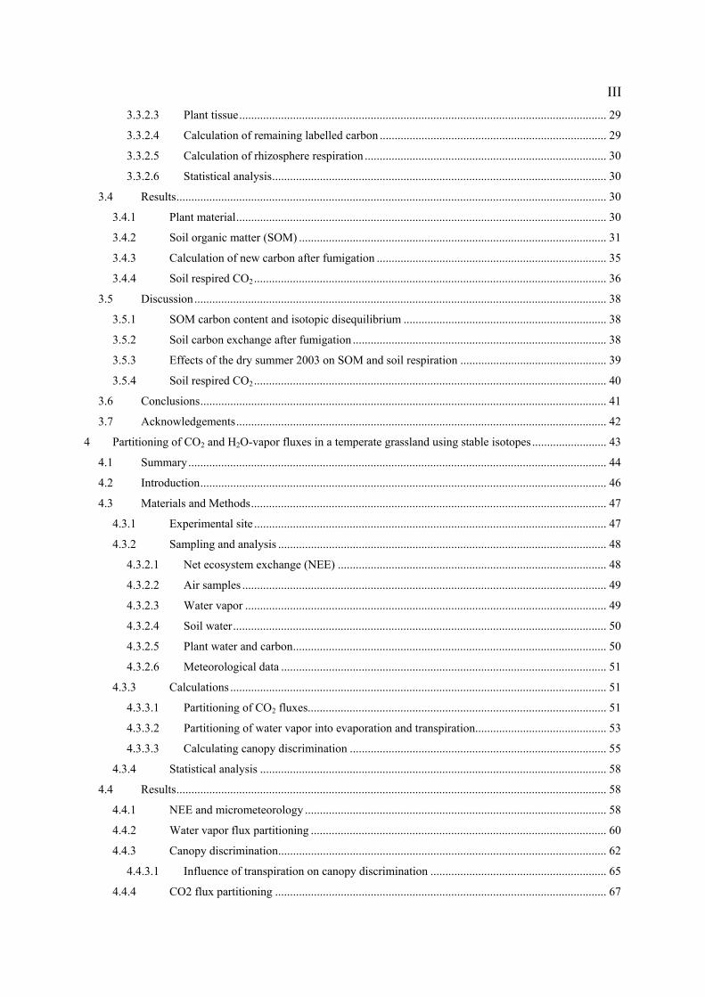
2.3 System design
2.3.1 Overview
The air sampler (ASA) is enclosed in a 60 cm x 55 cm x 75 cm portable weatherproof
aluminium case equipped with small wheels (Incas, Knörr AG, Germany) and weighs 55 kg
with the case. For sampling and storage of air, cylindric glass flasks (Keller Glas,
Switzerland) with a diameter of 6 cm, reducing to a 6 mm connection tube with manual
regulating valves on both ends, were used. The flasks have a volume of 300 mL each, in order
to obtain a sufficiently large air sample for trace gas analysis. Eleven of these flasks are
connected to a twelve position multiport valve (Valco multiport ST valve, VICI, USA) using
1/8” stainless steel tubes (VICI, USA). The twelfth position on the valve was connected to a
small loop. The rotor material used in the multiport valves was Valcon M (VICI, USA),
which is the most inert available in regard to isotopic exchange effects for 13C and 18O
(Schauer et al., 2003). Transition between glass flasks and stainless steel tubes was made with
6 mm to 1/8” connectors (Swagelok, USA) containing Teflon (PTFE) seals at the glass side.
Three identical multiport valves with eleven flasks each are set up in serial connection
through their inlets and outlets with flexible Teflon (PTFE) tubes, yielding a total of 33
sampling flasks (Figure 1). The system is built on four levels inside the aluminium case, three
levels each hold one multiport valve connected to eleven glass flasks. The fourth level holds
the pump, the electronic devices, and a front panel with the gas in- and outlets (Trigress,
Switzerland), control switches for power and the manual three way valves and a socket for the
electronic control cable. Positions of the multiport valves are fully computer controllable
making automated and unattended sampling and analysis possible. In the laboratory the ASA
is directly connected to the mass spectrometer and is computer controlled, like an
autosampler.

10
Figure 1 Diagram of the air sampler (ASA). A) magnet valve, controlling whether the pump draws air through the ASA (sampling state) or from the standby inlet (standby and release state). B) 3-way manually switchable valves to change between sampling mode or analysis mode. M1-3) multiport rotary valves connected to eleven sampling flasks each. The loop position serves as a bypass
2.3.2 Operation
A teflon membrane pump (811KNE, KNF, Germany) which is installed downstream of the
flowline pulls the air through the ASA resulting in a flow of 2 L min-1 (flow rate of the pump
without resistance is 11.5 L min-1). After passing a particle filter (Hepa-Vent, Whatman, UK)
and a MgCl2O8 drying column the air stream is subsequently directed to the desired sampling
flask according to the momentary positions of the three multiport valves M1-M3. Between the
last multiport valve M3 and before the pump, a magnet valve (EVT307-5T0-02F-Q, SMC,

11
Switzerland) switches between the flask line and a standby inlet (Figure 1). Between sampling
intervals, when no flask is to be filled, the air flows through the standby inlet and not the flask
line, preventing an early exhaustion of the desiccant. This is also thought to prolong the
lifespan of the pump since switching it on and off many times during sampling sessions
would most likely increase the risk of a breakdown. There are three states of the system:
standby state where the magnet valve opens the standby inlet while all multiport valves are on
the loop position, sampling state with the magnet valve switched to the flask line to fill the
selected flask. To fill e.g. flask number 14 on the second level, the multiport valves M1 and
M3 are set to the loop position, while multiport M2 is set to the appropriate flask position.
Finally the release state: the magnet valve is switched to the standby inlet while the multiport
valves remain in their position. This allows the equilibration of the pressure difference
between the flasks and the ambient pressure, which is a result of the pump operating in
downstream position. The system then goes back to the standby state.
The main outlet -after the three multiport valves- can be connected to an external infrared gas
analyzer (IRGA) for in situ measurements of the CO2 concentration of the individual samples.
With an additional computer controlled manifold connected to the input of the system,
automated sampling of several gas sources is possible, e.g. to sample height profiles in and
above a plant canopy (Figure 2). The current construction of the system allows sampling of
six gas sources. More inputs are possible, depending only on the construction of the
peripheral input manifold.
2.3.3 Computer control
2.3.3.1 Sampling
For gas sampling in the field, the ASA and its peripheral components (IRGA, gas input
manifold) are controlled with a LabView (National Instruments, USA) program running on a
portable computer. The main elements of this program include control over sampling intervals
and times, duration of the above mentioned system states, settings of the external gas input
manifold and logging of the IRGA data. The different devices require individual
communication protocols: the multiports M1-M3 are controlled with a modified RS485
protocol (semiduplex), the IRGA requires the RS232 protocol and finally the gas input
manifold is controlled with +12V pulses. An interface was developed to provide two-way
communication between the mentioned devices and the computer via one single RS232 or

12
USB port. The two-way communication enables the control program to verify the position of
the multiports M1-M3.
Figure 2 Schematic of the ASA and its peripheral components. Field situation with manifold and IRGA, and laboratory situation with precon and mass spectrometer.
2.3.3.2 Analysis
For laboratory use as an autosampler the three multiport valves are controlled by electric
impulse signals coming from the Gasbench II (Finnigan, Germany), a peripheral of the Delta
Plus XL mass spectrometer (Finnigan, Germany). Each multiport M1-M3 is switched via
pulse relais built into the Gasbench II, thus the ASA can be controlled from within the Isodat
Software (Version 2.0, Finnigan, Germany) used to control the mass spectrometer. This
allows integration into the specific analysis protocol within the Isodat Software. Two
interconnected but independent gas circuits on the used Precon-Device (Finnigan, Germany)
were deployed to program a nested analysis mode, cutting down analysis time significantly
(see below). A given sample is flushed from its flask by the Helium carrier gas at 50 mL min-1
for 380 seconds with the multiport of the Precon device in “load” position (Figure 3). For
cryofocussing with liquid nitrogen the multiport is switched to the “inject” position for 10
seconds and then back to “load”. Gas chromatographic separation and mass spectrometric
analysis take another 640 seconds, but instead of waiting for the sample to finish analysis

13
completely, 380 seconds before the end the next sample can already be flushed from its flask.
With this nested protocol 33 samples can be automatically analyzed for δ13C and δ18O
isotopic ratios of CO2 in 5 hours and 52 minutes, corresponding to 10 minutes and 40 seconds
per individual sample.
Figure 3 Schematic of the precon device with the gas flowpaths shown. The multiport has two switchable positions (load, inject) to control the carrier gas during analysis. The “load” position, as shown in the schematic, is used to flush the samples from the glass flasks in the ASA.
2.4 System performance
2.4.1 Calibration of the Mass Spectrometer
Calibration of the analysis system (mass spectrometer and used peripherals) for system related
offsets is done by injecting calibrated reference gas with every sample (one reference peak per
sample). Reference gas is 100% CO2 (Air Liquide, Switzerland) which itself was calibrated
with dual inlet analysis against a CO2 standard gas (Oztech, USA). To rule out possible
effects of the peripheral precon device during analysis the reference gas was tested against
itself. Results for δ13C and δ18O where consistent against the reference peak when injecting
the reference gas with a single glass flask through the precon device. The ASA itself was
tested against single glass flask analysis (see Table 2) to exclude the possibility of a system
related offset. Signal strength at mass 44 is 6 to 8 Volts for ambient CO2 concentrations.

14
2.4.2 Laboratory performance
The performance of the ASA for δ13CVPDB and δ18OVSMOW of CO2 in air was tested in the
laboratory. Compressed air (Carbagas AG, Switzerland) and compressed mixtures of
synthetic air (80% N2, 20% O2, Carbagas AG, Switzerland) with CO2 of different isotopic
ratios was used (Table 1). Sampling required a gas overflow which was maintained at >1 L
min-1 at the input of the ASA. The internal pump in the ASA generated a through flow of 2 L
min-1 and sampling flasks each were flushed with at least six-fold their volume. The
difference to ambient pressure in the flasks after flushing was immediately equilibrated
thereafter, as described above.
Table 1 Gas 1 is compressed air, gas 2 is a mixture of synthetic air (80% N2, 20% O2) with CO2 and gas 3 is a CO2 calibration gas (Carbagas, Switzerland). CO2 concentrations were measured with an IRGA (LI-COR 6262 CO2/H2O analyzer). Isotopic ratios are expressed in the δ notation with ± standard deviation (σ). Typical atmospheric values are given for comparison.
Gas 1 Gas 2 Gas 3 Air
CO2 (ppmv) 398.2 404.3 340.4 ~380
δ13C (‰) -9.42 ± 0.08 -45.57 ± 0.06 -29.16 ± 0.07 ~-9
δ18O (‰) 33.15 ± 0.08 8.33 ± 0.07 9.20 ± 0.04 ~33
The three different gases with CO2 concentrations in the range of ambient CO2 (Table 1) were
filled into the ASA in sequence (gas 1 in flask 1, gas 2 in flask 2, gas 3 in flask 3, gas 1 in
flask 4 and so forth) so that every flask had two neighboring flasks with different gases.
Isotope ratio determination was done within 6 hours after filling and showed good
consistency within the individual gases (Figure 4). Observed standard deviations (σ) were
between 0.06‰ and 0.08‰ for δ13CVPDB and between 0.04‰ and 0.08‰ for δ18OVSMOW . The
standard error (SE) representing the measurement precision was between 0.02‰ and 0.03‰
for δ13CVPDB and between 0.01‰ and 0.02‰ for δ18OVSMOW (n=11). These results lie within
the range of the instrument precision using the cryofocussing technique and show that effects
of possible leaks and mixing processes within the ASA are negligible on short term analysis,
thus offering the potential for high precision measurements of field samples.

15 Gas 1, 398.2 ppm CO2
Injection Number
1 4 7 10 13 16 19 22 25 28 31
δ 13
C (‰
)
-9.6
-9.4
-9.2
δ 18
O (‰
)
33.0
33.2
33.4mean = 33.15σ = 0.08SE = 0.02
mean = -9.42σ = 0.08SE = 0.03
a)
Gas 2, 404.3 ppm CO2
Injection Number
2 5 8 11 14 17 20 23 26 29 32
δ 13
C (‰
)
-45.4
-45.6
-45.8
δ 18
O (‰
)
8.1
8.3
8.5
mean = -45.57σ = 0.06SE = 0.02
mean = 8.33σ = 0.07SE = 0.02
b)
Gas 3, 340.4 ppm CO2
Injection Number
3 6 9 12 15 18 21 24 27 30 33
δ 13
C (‰
)
-29.5
-29.3
-29.1
δ 18
O (‰
)
9.1
9.3
9.5mean = 9.20σ = 0.04SE = 0.01
mean = -29.16σ = 0.07SE = 0.02
c)
Figure 4, a-c Carbon and oxygen isotope ratios of CO2 in a) compressed air, b) and c) synthetic air. The samples were collected with the ASA in sequence 1,2,3 1,2,3 and so forth. Standard deviation (σ) was between 0.04‰ and 0.08‰ and standard error (SE, n=11) between 0.01‰ and 0.03‰ for all samples.

16
2.4.2.1 Storage effects
Long time storage tests to evaluate for possible internal mixing, leakage or exchange effects
have been done with the same experimental setup as described above, using the gases 1-3.
The stopcocks of the glass flasks where left open during the experiments but for long time
storage of samples they can be closed if desired. Isotope ratio determination for δ13C and δ18O
of CO2 was done 8 days after sampling and in a second experiment 27 days after sampling
(Figure 5). Gas 1 proved to be relatively stable and showed changes of 0.07‰ ± 0.05‰ for
δ13C and 0.51‰ ± 0.03‰ for δ18O within 27 days. Compared to the initial measurements on
day zero gas 2 showed the largest variation regarding total drift as well as variation between
individual samples, being expressed by the standard deviation (σ) of 0.43‰ for δ13C and
0.34‰ for δ18O.
storage days0 5 8 10 15 20 25 27
δ13C
(‰),
diffe
renc
e to
day
zer
o
0
1
2
δ18O
(‰),
diffe
renc
e to
day
zer
o
2
1
0
gas1 13C
gas2 13C
gas3 13C
gas1 18O
gas2 18O
gas3 18O
Figure 5 Storage effects on CO2 stable isotopic composition. Horizontal line represents values at day zero for both δ13C and δ18O and error bars indicate ± standard deviations (σ, n=11).
The three gases behave quite differently regarding magnitude and scatter of the observed drift.
The largest variation was measured in gas 2, which is also the gas with the greatest isotopic
differences to atmospheric CO2 isotopic composition (Table 1). Gas 3 shows the second
largest variations and gas 1, which has a similar CO2 isotopic composition as the surrounding
air, is relatively stable over 27 days, in particular for δ13C. Therefore it can be assumed that
the cause of the drift is not internal mixing of gases inside the ASA, but exchange with
outside air through very small leaks. This most likely occurs at the transitions from the glass

17
flasks to the steel tubes which are sealed by Teflon (PTFE) ferrules. But since gas 1 and 2
have similar CO2 concentration gradients to ambient air, leakage can not fully account for the
observed difference over time between the two gases. Other factors such as surface exchange
effects with the used materials (glass, Teflon, stainless steel, valco rotor material) and
exchange effects with water inside the system could have influenced the experiments. The
magnitude of influence of each individual factor is unknown.
The data show that storage of samples is possible for about one week without the risk of
strong drifts or isotopic exchange effects during that time. Air samples from the field which
will usually have smaller differences to atmospheric isotopic composition than our test gases
should therefore be even much less affected during storage.
2.4.2.2 Automated compared to manual gas sampling and analysis
To compare for stability and consistence of the ASA analysis, δ13C and δ18O of CO2 was
determined with manual sampling and analysis technique, using the same type glass flask as
in the ASA. The same glass flask was used eleven times in sequence and was filled with gas 2
(Table 1) during two minutes at a flow rate of 1 L min-1 each time. For analysis the glass
flasks were connected to the Helium carrier gas flow of the Precon peripheral from the mass
spectrometer.
The results for both δ13C and δ18O show a good consistency for each of the methods (Table
2). Standard deviations where 2 to 6-fold larger with the manual analysis than with the ASA.
Peak areas also showed a much larger variation in the manual analysis, this exemplifies that
the automation of the ASA helps to provide more stable results (Figure 6). The offset of the
injection peak area between the two methods is due to a different analysis protocol for manual
and automated analysis (flushing times, freezing times).
Table 2 Comparison of ASA and single flask analysis
ASA single flask
δ13C (‰) δ18O (‰) δ13C (‰) δ18O (‰)
mean -45.57 8.33 -45.84 8.17
σ 0.06 0.07 0.13 0.42
SE (n=11) 0.02 0.02 0.04 0.13

18
Figure 6 Comparison of manual single flask to automated ASA analysis of gas 2. Black symbols are ASA measurements of δ13C (squares) and δ18O (circles) of CO2 (n=11). White symbols are single flask analysis of δ13C (diamonds) and δ18O (triangles) of CO2 (n=11).
2.4.2.3 CO and CH4 isotope analysis
To show a wider range of possible applications for the ASA in the field, performance was
tested with other carbon containing trace gases such as CO and CH4 with samples of
compressed air. These trace gases have lower atmospheric concentrations than CO2 (CO:
~100-500 ppbv, CH4: ~1.7 ppmv) and therefore require longer freezing times in the pre-
concentration step of the isotope analysis. CO was separated from other carbonic trace gases
using a Precon peripheral with a carbosorb (Hekatech, Germany) CO2 removal tube and
subsequent cryofixation of potentially not adsorbed CO2 and other condensable gases such as
H2O. CO is passing the liquid nitrogen trap and is then oxidized to CO2 with Schütze reagent
(Mak & Yang, 1998) contained in a downstream glass tube. The CO δ13C and δ18O isotopic
ratio could then be determined following CO2 analysis protocols. Standard deviation (σ) for
33 samples of compressed air was 0.17‰ for δ13CVPDB and the standard error (SE) 0.03‰
(n=33) showing a measurement precision within the detection limit (Figure 7). Since Schütze
reagent does not alter δ18O isotopic composition of the original CO it can also be quantified
after correction for O added by the reagent (Mak et al., 1998). δ18O of CO (data not shown)
had a standard deviation (σ) of ± 0.20‰ and a standard error (SE) of 0.04‰ (n=33), again
exemplifying a good measurement precision.

19
CO in compressed air
Flask Number
0 5 10 15 20 25 30 35
δ 13
C (‰
)
-35
-34
-33
-32
-31
mean = -33.49σ = 0.17SE = 0.03
Figure 7 Carbon δ13C isotopic ratios of CO (370 ppbv) in compressed air.
Similarly as for CO, CH4 from compressed air samples needed to be separated from CO2
during analysis using a Precon peripheral. After oxidation of CH4 to CO2 at 1050°C standard
CO2 analysis protocols were followed for δ13C isotopic ratio determination. Results of CH4
δ13C showed a linear drift with an r2 of 0.85, enabling calibration with the use of appropriate
standards. Variation around the calculated drift had a standard deviation (σ) of 0.39‰ and a
standard error (SE) of 0.07‰ (n=33) (Figure 8). The drift in δ13C does not seem to be directly
related to the ASA as a sampling device since this has been observed on other occasions in
our laboratory using manual single flask analysis for CH4 δ13C (data not shown).
CH4 in compressed air
Flask Number
0 5 10 15 20 25 30 35
δ 13
C (‰
)
-48
-47
-46
-45
-44
-43
-42
r2= 0.85σ = 0.39SE = 0.07
Figure 8 Carbon δ13C isotopic ratios of CH4 in compressed air (1.7 ppmv). A linear drift (r2 = 0.85) of δ13C during analysis was observed. Solid line is linear regression and dashed lines are ± standard deviation (σ = 0.39‰).

20
2.4.3 Field performance
Air samples were collected at the grassland experimental site of the Federal Institute of
Technology (ETHZ) in Eschikon near Zurich (8°41’E, 47°27’N). Monocultures of Lolium
perenne are used to investigate carbon fluxes in a fertile grassland ecosystem under field
conditions. An open-flow chamber system is used to measure net ecosystem CO2 exchange
and collect air samples for carbon δ13C isotopic ratios of CO2. The chamber which is 0.6 m
high and covers a square area of 0.49 m2 consists of an aluminium framework covered with
transparent Teflon (PTFE) film except for the side for the inlet and outlet which is made of
Plexiglas ( see Aeschlimann, 2003 for further description). Air samples were collected from
the in- and outlet of the chamber during a 24 hour period on May 18th 2003 using two ASA
at the outlet of the ASA. Calibration grade gas (Messer-Griesheim) was used to
ling and synthetic air (Carbagas AG, Switzerland) served as
devices, yielding a total of 66 samples. CO2 concentration was measured in situ by connecting
an IRGA
calibrate the IRGA before samp
zero-calibration and as reference gas during the CO2 concentration measurements. Air
samples were analyzed for δ13C isotopic ratios of CO2 in the laboratory within 24 hours. A
Keeling Type plot where the carbon δ13C isotopic ratios of CO2 are plotted against the inverse
of the CO2 concentration showed a correlation of 0.99 (r2) between the individual samples
(Figure 9).
Grassland (L. perenne) Keeling Type Plot
1/[CO2] (ppmv-1)
0.0024 0.0026 0.0028 0.0030
δ 13
C (‰
)
-11
-10
-9
-8
-7
-6
-5y=7286.4x - 27.4r2=0.99n=66
Figure 9 Keeling type plot analysis of the carbon δ13C isotopic ratios of CO2 with linear regression line (r2 = 0.99, n = 66). Samples represent a 24 hour period.

21
2.5 Conclusions
The ASA and its peripheral components offer the possibility to collect a large number of air
samples with a mobile and automated device. High precision analysis for stable isotopes of
various carbon containing trace gases can be carried out in a fast, reproducible and reliable
manner. Furthermore the sampling unit can be directly connected to the mass spectrometer
with two carrier gas lines leading to the Precon peripheral and a hardware plug for the
electronic control of the ASA.
Since no glass flasks need to be removed from the sampler, a reproducible and fast analysis of
the air samples in the flasks is possible. Furthermore, the potential contamination of the air
samples is avoided by leaving the glass flasks in place. This saves much time and reduces the
potential for errors during handling. The relatively high costs for the automated multiport
valves are soon compensated for by reduced costs for personnel during field and lab work.
aking the results more reliable. The necessary measurements of the
rried out by means of a chamber system as
The system will be a useful tool to further investigate ecosystem carbon fluxes with a high
sampling frequency thus m
net ecosystem exchange (NEE) can either be ca
described above or by applying the eddy covariance technique. It could be shown that the
ASA is also a useful tool for trace gas sampling and analysis for gases with concentrations up
to 1000 times less than that of CO2. Applications for non-carbon containing trace gases, such
as nitrous or sulphurous oxides, also seem possible – limited only by preparation peripherals
and the analyzing capabilities of the involved mass spectrometer.
2.6 Acknowledgements
This study is supported by the COST 627 initiative “Carbon storage in European Grasslands”
(Grant No. C01.0056), Federal office for education and Science. Thanks for technical help
and advice to Robert Widmer. Thanks to Eva Bantelmann for help with the assembly of the
ASA. Thanks also to April Siegwolf for proofreading the manuscript.

22
Chapter 3
3 Dynamics of soil organic matter turnover and soil respired CO2 in a temperate grassland labelled with carbon-13
Submitted to European Journal of Soil Science

23
The fate of carbon in grassland soils is of particular interest since 98% of the carbon in
rassland ecosystems is stored belowground and respiratory carbon release from soils is a
major component of the global carbon balance. The use of 13C depleted CO2 in a ten year free
turn
of the proportional contribution of rhizosphere respiration to total soil respiration. SOM, soil
air a were analysed for δ13C and carbon content in the last year of the FACE
xperiment (2002) and in the two following growing seasons. After ten years of CO2
nrichment conditions to 600 ppm no significant differences in SOM carbon content could be
etected between fumigated and non fumigated plots. A 13C depletion of 3.4‰ was found in
SOM (0-12 cm) of the fumigated soils in comparison to the control soils and a rapid decrease
of this difference was observed after the end of fumigation. After two years a calculated 45%
of the carbon in SOM (0-12 cm) had been replaced by fresh carbon and annual input was
estimated to 9.8 ± 3.7 Mg ha-1. Rhizosphere respiration was calculated to 61% of total soil
respiration, this is similar to recent findings in forest soils. Consideration of ecophysiological
factors which drive plant activity is therefore important when soil respiration is to be
investigated or modelled.
3.1 Summary
g
air carbon dioxide enrichment (FACE) experiment, gave a unique opportunity to study the
over of the carbon sequestered during the FACE experiment and also allowed an estimate
nd plant material
e
e
d

24
3.2 Introduction
C3 plants (Balesdent et al., 1987). In our study, the use of C
depleted CO2 of fossil origin in a ten year “free air carbon dioxide enrichment” (FACE)
experiment, caused a strong 13C label within the soil (see Jones et al., 2004). The 13C
disequilibrium of SOM and plants after the end of the CO2 enrichment gave a unique
opportunity to calculate annual inputs of new carbon and to study soil processes like
rhizosphere respiration, which are driven by the aboveground plants.
A large proportion of carbon that enters the soil is returned to the atmosphere by soil
respiration (Jones et al., 2004) and it is therefore considered a key factor for soil carbon
turnover. Soil respiration has two major sources: heterotrophic microbial respiration of SOM
and rhizosphere respiration. For the latter, the definition of Ekblad & Högberg, 2001 is used:
rhizosphere respiration is regarded as the sum of respiration by living roots, their associated
mycorrhizal fungi and heterotrophic respiratory transformation of root exudates. The
proportions of the individual contributions to soil respiration are still uncertain; only few
studies have been done. For grassland, rhizosphere respiration was reported to account for 16
to 95% of total soil respiration (Jones et al., 2004). In forest ecosystems, rhizosphere
respiration was recently found to be the dominating factor in soil respiration (Ekblad et al.,
Temperate grasslands cover about 20% of the land area in Europe (Soussana et al., 2004). In
these ecosystems up to 98% of the total carbon can be found belowground (Hungate et al.,
1997). In general, soil organic matter (SOM) contains twice the amount of carbon found in
the atmosphere (Post et al., 1982). Within the context of the expected future changes of
climatic conditions and rising atmospheric CO2 content it is still uncertain if the soil carbon
pools will be a future source or sink.
Newly introduced carbon into soils is predominantly be found in coarse fractions (Balesdent
et al., 1987, Van Kessel et al., 2000, Xie et al., 2005). Non-hydrolysable soil fractions which
mainly consist of stable humus are soil carbon pools with a very slow turnover rate and are
therefore conservative in regard to new carbon input (Pelz et al., 2005). Freshly introduced
carbon, for instance after land use has changed from arable to grassland, is mainly sequestered
into labile carbon pools. If land use is changed back to arable again, the previously
accumulated carbon is released readily (Soussana et al., 2004).
Balesdent calculated the introduction of new carbon into a soil where newly grown C4 plants
caused a gradual change in 13C isotopic composition of SOM on a field that previously was in
isotopic equilibrium with 13

25
2001, Högberg et al., 2001). Measurements by Soe in a sugar beet field under FACE
action of rhizosphere respiration to be 70% (Soe et al., 2004). In
ot respiration within total soil
conditions showed the fr
contrast, Buchmann concluded microbial SOM respiration to be the dominating factor in
stands of Picea abies (Buchmann, 2000). No standard method has yet been established,
currently several techniques are being used (soil CO2 evolution, soil air, tree girdling) based
on 13C measurements. The question also remains how similar grassland and forest soils are
regarding the individual proportions (rhizosphere and SOM respiration) within total soil
respiration.
Photosynthetic activity of aboveground plant components, and therefore also
micrometeorological conditions, seems to be a driving force for soil respiration. Numerous
studies showed that the δ13C of soil respired CO2 is subject to seasonal changes (Ekblad et al.,
2005, Flanagan et al., 1996, Steinmann et al., 2004) and a close link to short term weather
conditions was found (Bowling et al., 2002, Ekblad et al., 2001). High air temperatures and a
large vapour pressure deficit (VPD) cause plant drought stress and stomatal closure
(Scheidegger et al., 2000). This decreases the proportion of ro
respiration, leading to an increase in δ13C of soil respired CO2 (Ekblad et al., 2001). In our
study, the monitoring of soil respired CO2 over three growing seasons gave the opportunity to
analyse the impact of a drought period (summer 2003) on the soil CO2 system and to calculate
the proportional contribution of rhizosphere respiration to total soil respiration.
The goals of this study are
• to determine how fast the carbon which was sequestered during the CO2 exposure has
been replaced with fresh carbon after the FACE experiment, without a change in land
use
• to evaluate the proportional contributions of rhizosphere respiration to total soil
respiration
• to track seasonal changes in δ13C of soil CO2 and to assign the driving environmental
factors

26
ide Enrichment (FACE) technology (Hendrey, 1992). The experiment was set up
3.3 Materials and methods
3.3.1 Experimental site
The Swiss FACE site in Eschikon (8º41‘E, 47º27‘N) is located near Zurich at an altitude of
550 m above sea level. To study the impact of elevated CO2 on a managed grassland
ecosystem, monocultures of Lolium perenne have been fumigated to an average of 600 ppm
CO2 (± 10% over 92% of the fumigation time) during ten growing seasons using Free Air
Carbon diox
in three replicates of fumigated and non-fumigated control plots (diameter per plot: 18 m).
CO2-fumigation was started in May 1993 and maintained from March to November at
daylight hours until discontinuation in November 2002 (see Zanetti et al., 1996 and Hebeisen
et al., 1997 for further description). The added CO2 from the fumigation tank was 13C
depleted since it originated from the combustion of fossil C-sources (-28.8‰ δ13C of CO2 in
2002). This resulted in a calculated average value in 2002 of -16‰ for δ13C in the CO2
enriched air of the fumigated plots as compared to -8‰ in the control plots, according to the
mass balance (see also equation 4):
face
tankafaceaaface c
ccc )δ(δδ
−+= (1)
wit a
isotopi
isotopic value within a FACE ring during fumigation.
The o
the standard Vienna Pee Dee Belemnite (VPDB):
h c being ambient and cface being the CO2 concentration in the FACE rings. δa is the
c value of ambient, δtank of the CO132 from the fumigation tank and δface the calculated
is topic composition of the stable isotope 13C is expressed in the δ unit (‰), relative to
2
122
1313
COCOR with 1000* 1
RR(samp⎡Cδ
(standard)
le)=⎥
⎦
⎤⎢⎣
−= (2)
addition to the elevated CO2 application, and maintained until 2004, all plots were
rtilized each year with 55 kg P ha-1 and 241 kg K ha-1 to compensate for harvest losses. Two
eatments of nitrogen (N) fertilization were applied (140 and 560 kg ha-1 a-1, as NH4NO3). L.
In
fe
tr

27
ear and all sampling was done shortly before harvest to
avoid any effects of cutting, in particular on soil air CO2. The soil is classified as an eutric
silt, 310 g kg-1 sand and 300 g kg-1 clay in the top 0-10 cm
cm in length were sampled and immediately split into
ree sections (0-3 cm, 3-6 cm and 6-12 cm). The samples were kept in airtight glass tubes
(L18, Schott, Germany) and frozen at -20 °C within 24 hours. Further processing was done
within three months after sa
move roots (mesh size: 630 µm) and ground to powder with a ball mill (Retsol MM2000,
f the 2002 samples as compared to the
ixed with 40 µl 2.5 M HCl. After
4 hours the aliquots were washed twice with 40µl H2O to remove remaining HCl. Analysis
for carbon (C) and nitrogen (N) content and δ13C value of C was done by combusting the
samples to N2 and CO2 in an Elemental Analyzer (Carlo Erba 1
ass spectrometer via the CONFLOII interface (both Thermo Electron, former Finnigan 15
perenne swards were cut five times a y
Cambisol, containing 390 g kg-1
with a pH of 7.1. Bulk density for 0-10 cm soil depth is 1.2 ± 0.2 g cm-3 (Van Kessel et al.,
2000).
3.3.2 Sampling and analysis
Soil, soil air and plant tissue samples were collected on six occasions from September 2002 to
October 2004. A single field campaign lasted for 10-15 days during which all three FACE
replicates were sampled. The N treatments were two subplots in the six plots; this gave a total
of twelve sampling areas in each field campaign. Exceptions were May 2004 for soil air and
September 2002 plus May 2004 for bulk soil samples when only the subplots (high and low N
treatments) of one fumigated and the corresponding control plot were sampled.
3.3.2.1 Bulk Soil
Soil cores 2 cm in diameter and 12
th
mpling. Samples were dried at 80 °C and 10-2 mbar, sieved to
re
Rentsch, Germany). An exception were the soil samples from 2002 which did not undergo the
sieving process but only had visible plant material such as fine roots removed manually. This
resulted in higher carbon concentrations within some o
sieved ones from 2003 and 2004. To remove any traces of carbonate (Ca2CO3) an aliquot of
20 mg of each sample was weighed in silver capsules and m
2
108, Italy) coupled to a Delta
S m
MAT, Germany) in continuous-flow mode. Since the soil was (unevenly) labelled with N
from a previous experiment, analysis for δ15N was not performed. The achieved precision for
repeated analysis of a standard material was ±0.1‰ for δ13C (standard deviation, σ). The
relative precision for C and N content was ±2% (σ).

28
nd highest values of the respective depths from 2003 and 2004, including the standard
errors. This interval, defined by the lowest and highest boundaries of the standard errors, was
e calculated values. Correction of δ13C was done along
ng season and at least seven days prior to sampling brass tubes
ameter) were inserted vertically into the soil (depth: 12 cm), leaving a
hter 12C, leaving a 13C enriched air mass
behind.
All samples from the control plots and the 0-3 cm samples from the fumigated plots from
2002 were corrected for carbon content and δ13C due to the additional carbon they contained
(see above). The new carbon content was the calculated mean of the interval defined by the
lowest a
subsequently used as error bar for th
the characteristic curves from Figure 10, using the same interval and thus calculating a new
lower and upper boundary for δ13C (used as error bar subsequently) and the mean thereof.
Control plot samples were corrected according to δ13C = -1.39*C% -26.67 and the topsoil
fumigated samples according to δ13C = -5.53*C% -26.14 (see Figure 10).
3.3.2.2 Soil air
At the beginning of the growi
(15 cm long, 3 cm di
hollow space inside the tubes. The top was closed airtight with a rubber plug covered with
Teflon (PTFE) foil. The tubes had two opposing slits of 6 cm length to integrate soil air from
6 to 12 cm below the surface and were open at the bottom. Sampling was done by inserting a
needle through the rubber plug and pulling 15 ml of air from the tubes into the syringe. The
air samples were immediately transferred into evacuated 12.5 ml Vacutainers (LABCO
Exutainers, Medical Instruments Corporation, Switzerland) and analyzed within 24 hours
using a Gasbench II periphery connected to a Delta Plus XL mass spectrometer (both Thermo
Electron, former Finnigan MAT, Germany). Samples with a CO2 concentration of less than
850 ppm were discarded (4 of 235). Repeated measurements of a standard gas using the
cryofocussing technique for CO2 have a precision of ±0.1‰ (σ) on δ13C of CO2 and a relative
precision of ±1% for CO2 concentration.
Samples of soil air can have a CO2 concentration ranging from almost ambient to several 10
000 ppm. To calculate the δ13C of soil respired CO2 (source value) a two component mixing
model was applied (Keeling, 1958), where the δ13C value (y-axis) is plotted against the
inverse of the CO2 concentration. The y-intercept is the isotopic value of the source CO2 with
a diffusional enrichment of 4.4‰ (Amundson et al., 1998). The offset of 4.4‰ between the
mean δ13C value of the respired carbon sources and the calculated source (from the mixing
model) arises from the more rapid diffusion of the lig
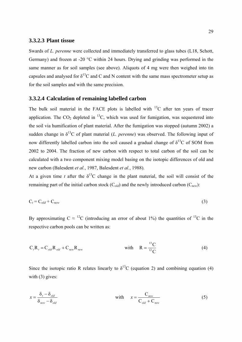
29
as sequestered into
ation of plant material. After the fumigation was stopped (autumn 2002) a
sudden change in δ13C of plant material (L. perenne) was observed. The following input of
3.3.2.3 Plant tissue
Swards of L. perenne were collected and immediately transferred to glass tubes (L18, Schott,
Germany) and frozen at -20 °C within 24 hours. Drying and grinding was performed in the
same manner as for soil samples (see above). Aliquots of 4 mg were then weighed into tin
capsules and analysed for δ13C and C and N content with the same mass spectrometer setup as
for the soil samples and with the same precision.
3.3.2.4 Calculation of remaining labelled carbon
The bulk soil material in the FACE plots is labelled with 13C after ten years of tracer
application. The CO2 depleted in 13C, which was used for fumigation, w
the soil via humific
now differently labelled carbon into the soil caused a gradual change of δ13C of SOM from
2002 to 2004. The fraction of new carbon with respect to total carbon of the soil can be
calculated with a two component mixing model basing on the isotopic differences of old and
new carbon (Balesdent et al., 1987, Balesdent et al., 1988).
At a given time t after the δ13C change in the plant material, the soil will consist of the
remaining part of the initial carbon stock (Cold) and the newly introduced carbon (Cnew):
Ct = Cold + Cnew (3)
By approximating C ≈ 12C (introducing an error of about 1%) the quantities of 13C in the
respective carbon pools can be written as:
CR with RCRC RC 12=+= newnewoldoldtt (4)
Since the isotopic ratio R relates linearly to δ
C13
13C (equation 2) and combining equation (4)
with (3) gives:
δδδδ
oldnew
oldtx−
= with −
newol
newxCC
C+
= (5) d

30
Since equation (5) basically describes the mixing of two differently labelled substances it may
and CO2 derived from plant root 13
where x is the fraction of new introduced carbon by the plants, δt the δ13C value of SOM at
time t, δold the δ13C value of SOM at the starting point and δnew the δ13C of the plant material
introducing the new label.
3.3.2.5 Calculation of rhizosphere respiration
also be used to separate CO2 derived from SOM respiration
and rhizosphere respiration if the plant material has a strong enough C label. For this case
equation (5) is rewritten to:
δδδδ
'SOMplants
SOMsoilairx−−
= (7)
with x' as the fraction of plant derived CO2 within the soil. δsoilair is the δ13C value of soil
respired CO2 minus the 4.4‰ offset (see above), δSOM the δ13C value of SOM in 6-12 cm
.3.2.6 Statistical analysis
onlinear regressions using an exponential decay function ( ) were done using
nt were analysed using ANOVA of the statistical
oftware R (R 2.0.1, GNU public license). Soil samples from the year 2003 were analysed
including the three replicates of fumigated and the corresponding control plots as described
above. Samples from 2002 and 2004 did not have all replicates at all times, so replication was
ot considered as a factor in the ANOVA for these years.
.4.1 Plant material
δ13C values of
incorporated during growth. A natural offset in δ13C, which is species and carbon fixation
depth (since soil respired CO2 is measured in this depth). δplants denotes the δ13C value of the
plant material.
3kte(t) −= 0δδN
Sigma Plot version 8 (SPSS Inc.). The sum of the residuals was < 0.004 in all cases.
Treatment effects of the FACE experime
s
n
3.4 Results
3
plant tissue represent an integrated isotopic signature of the CO2 being

31
athway dependent (C3 or C4), has its origin in the photosynthetic 13C discrimination, which is
ifference is reflected in the δ13C of the plant material: during
fumigation δ13C of plants was -37.4 ± 0.1‰ and with no fumigation -28.3 ± 0.1‰. ANOVA
the former fumigation on δ13C of L.
eved soil fractions (<630 µm, 0-12 cm soil depth) varied between
8 and 46 Mg C ha-1 (Table 3). Nitrogen was found in amounts of 4 to 5 Mg N ha-1.
Differences between treatm
of the individual sam
p
mainly caused by the enzyme RUBISCO (Farquhar et al., 1989). Fumigation resulted in a
δ13C value of CO2 (-16‰), which was 8‰ more negative than average values of the free
troposphere (-8‰). This d
revealed no significant effects of either N fertilisation or
perenne in 2003 and 2004.
3.4.2 Soil organic matter (SOM)
The carbon contents of the si
3
ents and years were not significant (ANOVA) due to the scattering
ples. C:N ratio was calculated to 8.8 ±0.1 as an average for all samples.
Table 3 Carbon and nitrogen content of the <630 µm soil fraction, 0-12 cm soil depth
C /Mg ha-1 N /Mg ha-1
2003 fumigated 41.0 ± 12.8 4.6 ± 1.2
control 38.0 ± 11.1 4.4 ± 1.0
2004 fumigated 46.4 ± 10.1 5.3 ± 1.0
4.6 ± 0.6 control 40.6 ± 6.8
13
soil depths (p<0.01) in 2003. The interaction between soil depth and CO
The effect of the former CO2 fumigation on δ C of SOM was still highly significant in all
same time δ13C showed an increase
11). Soil depth profiles from fumigated plots increased stronger (1.8‰
maximum) compared to the control plots, where change with depth was three-fold smaller
e of a linear regression of δ13C versus ln(%C) (Figure 10) denotes
2 fumigation (as co-
factor) was also significant (p < 0.05), showing that in each depth CO2 fumigation had a
different effect (see also Figure 11). Nitrogen fertilisation (140 and 560 kg ha-1 a-1) had no
significant effect on δ13C of SOM. No significant differences were measured between the
three field campaigns from May 2003, August 2003 and September 2003.
Carbon content of SOM decreased with depth while at the
(Figure 10, Figure
(0.6‰ maximum). The slop
the isotopic fractionation factor (O'Leary, 1981) which is a characteristic for a soil (Bundt et
al., 2001, Nadelhoffer & Fry, 1988). In undisturbed soils an increase of δ13C with depth is

32
observed (Nadelhoffer et al., 1988). Older SOM, on which only more specialised soil
microorganisms can feed, is slightly enriched in 13C (Figure 11). The soils that have been
fumigated with fossil CO2 show a much steeper gradient (Figure 10) for the reason that the
newly introduced organic matter is strongly depleted in 13C. In this case, the fractionation
factor is a measure of the isotopic disequilibrium within the soil profile.
%Ce
-26
0 e0 e1 e1 e1
-36
-34
-28
δ 13
C [‰
]
-38
-32
-30
2 3 4 5 6
Control
2002
2003 Fumigated2004
probable targe uet equilibrium valplants 2002(fumigated)
plants 2002 (control),2003 and 2004
y=mx+qm = -5.53q = -26.14r ² = 0.98
igure 10 Relationship of δ13C and carbon content of SOM with linear regressions (isotopic fractionation
th an r2 of 0.88 and
Ffactors). Means of each year, separated into three depths (0-3 cm, 3-6 cm, 6-12 cm) are shown, data points from 2002 are single observations. Encircled data points and all control data from 2002 samples show higher C contents than data from other years (see below). Black symbols are fumigated (2002) or formerly fumigated plots (2003 and 2004), white symbols are control plots. Plant δ13C values of fumigated (2002) and non-fumigated plots are depicted on the y-axis, box is mean ± standard error (SE, n=24 for 2002 fumigated and n=172 for 2002 control and 2003, 2004). Error bars for soil data are SE (2003 n=20, 2004 n=11).
The control soils are expected to be in isotopic equilibrium with the respective plant material
and all data pooled resulted in a linear relationship for δ13C and ln(%C) wi
p < 0.001. Soils from fumigated plots were in isotopic disequilibrium since it is assumed that
no new isotopic equilibrium has been reached after ten years of fumigation (2002), or within
the two years after the fumigation was stopped (2003, 2004). The probable target equilibrium
value for the fumigated soils (if fumigation would have continued until a new equilibrium is
reached) is proposed in Figure 10 and Figure 11. The line represents an estimate based on the
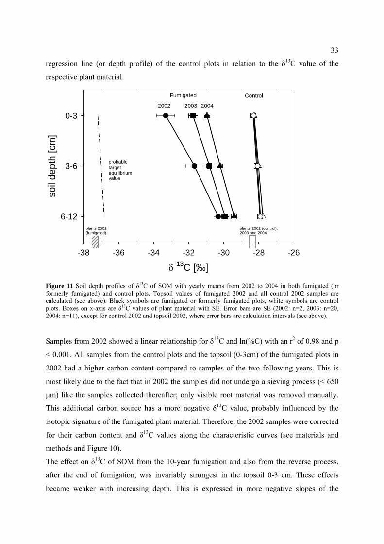
33
regression line (or depth profile) of the control plots in relation to the δ13C value of the
respective plant material.
δ 13C [‰]-38 -36 -34 -32 -30 -28 -26
soil
dept
h [c
m]
0-3
3-6
6-12
2002 2003 2004
Fumigated Control
plants 2002(fumigated)
plants 2002 (control),2003 and 2004
probabletargetequilibriumvalue
Figure 11 Soil depth profiles of δ13C of SOM with yearly means from 2002 to 2004 in both fumigated (or formerly fumigated) and control plots. Topsoil values of fumigated 2002 and all control 2002 samples are calculated (see above). Black symbols are fumigated or formerly fumigated plots, white symbols are control plots. Boxes on x-axis are δ13C values of plant material with SE. Error bars are SE (2002: n= 2003: n=20, 2004: n=11), except for control 2002 and topsoil 2002, where error bars are calculation intervals (see above).
ears. This is
ost likely due to the fact that in 2002 the samples did not undergo a sieving process (< 650
became weaker with increasing depth. This is expressed in more negative slopes of the
2,
Samples from 2002 showed a linear relationship for δ13C and ln(%C) with an r2 of 0.98 and p
< 0.001. All samples from the control plots and the topsoil (0-3cm) of the fumigated plots in
2002 had a higher carbon content compared to samples of the two following y
m
µm) like the samples collected thereafter; only visible root material was removed manually.
This additional carbon source has a more negative δ13C value, probably influenced by the
isotopic signature of the fumigated plant material. Therefore, the 2002 samples were corrected
for their carbon content and δ13C values along the characteristic curves (see materials and
methods and Figure 10).
The effect on δ13C of SOM from the 10-year fumigation and also from the reverse process,
after the end of fumigation, was invariably strongest in the topsoil 0-3 cm. These effects

34
The sudden change in δ13C of the plant material after the fumigation had significant effects on
δ13C of SOM (p < 0.05) in all investigated depths already in the first year after fumigation
(Figure 11). The change in δ13C from 2002 to 2003 was strongest in the topsoil level (+ 1.6‰)
and diminished with increasing depth. The same, yet less pronounced pattern could be seen in
the second year (2003 to 2004) where δ13C of the topsoil level increased by 0.7‰. The δ13C
values in the control plots stayed within ± 0.1‰ (SE) for a given depth in all three years and
showed a consistent increase of 0.4‰ from topsoil to the 6-12 cm layer in all three years.
regression lines from fumigated plots (-5.7 to -5.0) as compared to control plots (-1.4) in
Figure 10.
date(mm-yy)0 182 364 546 728 910
δ 13
C [‰
], di
ffere
nce
0
1
2
3
4
5
09-02 09-03 09-04
r2 = 0.62
End of fumigation
r time yielded an r2 of 0.62 with p = 0.06 (Figure 12). The time, after
Figure 12 Differences in δ13C of SOM between fumigated and control plots (means) from integrated values over 0-12cm soil depth. The curve is the best fit of an exponential decay function. Error bars are derived by error propagation based on the SE of the mean values.
The difference in δ13C of SOM between the fumigated and the control plots changed over
time and with depth (Figure 11). An exponential decay function fitted to the δ13C differences
in 0-12 cm soil depth ove
which the difference in the δ13C signal is halved, was calculated to 960 days (with 690 to
1570 days as 95% confidence interval). This means that in a little less than three years the

35
e signal we found at the end of the ten year fumigation period.
difference in δ13C between the fumigated and the control plots in 0-12 cm depth is calculated
to be half th
Samples from the August 2003 field campaign tended to show a larger difference than
expected from the model. Control samples from August 2003 were 1.0 ±0.2‰ less negative
than the other samples from 2003, resulting in larger differences for August 2003. These are
the samples taken during the exceptionally hot and dry summer experienced throughout
Europe (Figure 13).
Figure 13 δ13C of soil air, means of Keeling plot intercepts from the three FACE-plot replicates. Shaded bars are monthly means of precipitation and the curve is the temperature from a nearby station (Zürich, MeteoSchweiz). Error bars are SE from means; no error bars where not all three replicates were sampled (0504).
.4.3 Calculation of new carbon after fumigation
h
and to 9.6 ± 2.1 Mg ha-1 for the second year after fumigation.
3
Introduction of new carbon into the soil was calculated for the two years after fumigation
according to equation (5). In all three analysed soil depths the fractions were similar with an
associated error of 10-15% (Table 4). In the first year a maximum of 31% of new carbon was
found and in the second year t e (cumulative) amount of new carbon was 47% at maximum.
Annual new carbon input was estimated to 9.9 ± 3.1 Mg ha-1 in the top 12cm for the first year

36 Table 4 Cumulative fractions of new carbon sequestered after 2002 for three soil depths
depth 2003 2004
0-3 cm 0.31 ± 0.10 0.47 ± 0.10
3-6 cm 0.26 ± 0.15 0.43 ± 0.15
6-12 cm 0.20 ± 0.12 0.45 ± 0.12
3.4.4 Soil respired CO2
Soil respired CO2 showed a strong seasonal pattern in δ13C values (Figure 13), with a
maximum variation in δ13C between -25.1 to -21.6‰ (May to August 2003). Dry and hot
conditions tend to lead to more positive δ13C values (Steinmann et al., 2004); this is reflected
in the samples of August 2003. The summer period in 2003 showed monthly mean
temperatures of 23°C for June and August with at the same time very little precipitation of 58
and 82 mm respectively (Figure 13). Thirty year means for June are 15°, 124 mm and for
August 17°, 133 mm (MeteoSchweiz). As also seen in the SOM samples, the difference in
δ13C values between the control and the fumigated plots in August 2003 was larger compared
to the findings in the preceding campaign in May 2003 (Figure 14).
To eliminate seasonal effects, the differences between control and fumigated plots were
calculated and showed a general decrease over time (Figure 14). An exponential decay
function was fitted to the data and the rate constant k was 2.5-fold higher than the one
calculated for SOM in the topsoil level. This is mainly due to the sharp decrease in soil
respired CO2 δ13C differences after the first year, from 6.7 to 2.9‰. Such a strong change
could not be found in the SOM samples. The effect of fumigation (2002) on soil respired CO2
e it was only
bserved in 2002. During fumigation (2002) the difference in δ13C of the plant material from
-12cm depth SOM 3.4‰. Soil
respired CO showed a difference of 6.7‰ between fumigated and control plots, this implies a
r
was much stronger than the effect on SOM (Figure 15). There is a 3.3‰ offset from the 1:1
line which must have been caused by a direct or indirect effect of fumigation sinc
o
fumigated and control plots was 9.1‰ and the difference for 0
2
substantial influence of rhizosphere respiration on δ13C of soil respired CO2. This effect was
most clearly visible in 2002, since the isotopic disequilibrium was most expressed in the last
year of fumigation (Figure 11). In 2003 and 2004 δ13C of plant material was again much
closer to δ13C of SOM and the detectable effect of root respiration on δ13C thus became
smaller and is masked by the scattering of the samples (Figu e 15).

37
End of fumigation
dry summer
date(mm-yy)0 182 364 546 728 910
δ 8
13C
[‰ffe
renc
e],
di
0
2
4
6r2 = 0.85
End of fumigation
09-02 09-03 09-04
Figure 14 differences in δ13C of soil air between fumigated and control plots. Curve is the best fit of an exponential decay function. Error bars are derived by error propagation based on the SE of the mean values.
soil air δ 13C [‰], diff control - fumigated
1 2 3 4 5 6 7 8
SO
M δ
13C
[‰],
diff
cont
rol -
fum
igat
ed
1:1 line4
1
2
3
2002
Figure 15 Differences between fumigated and control plots of soil air δ13C against differences of SOM δ13C (0-12cm depth). White point is from 2002, black points are from 2003 and 2004. Error bars are SE.
The proportion of rhizosphere respiration within total soil respiration in the year 2002
(fumigated plots) was calculated to 61 ± 10% according to equation (7). For this calculation a
-4.4‰ offset in soil respired CO2 was included (Amundson et al., 1998) and the isotopic
values for SOM were taken from 6-12 cm depth; the same depth where the soil CO2 was
sampled from.

38
3.5 Discussion
3.5.1 SOM carbon content and isotopic disequilibrium
No significant difference in soil total organic carbon content between fumigated and control
plots was observed. This is in agreement with previous findings after six and nine years of
fumigation by Six et al., 2001, Van Kessel et al., 2000, Xie et al., 2005. The carbon content
of the soil in our study was similar to that observed by the above authors after six years of
fumigation although a direct comparison of the soil carbon content cannot be made, since
different pre-treatments were applied in each study plus the analysed depths were slightly
different (0-12 cm as opposed to 0-10 cm).
Soils from fumigated plots were found to be in strong isotopic disequilibrium with respect to
the plant canopy. Compared to a 2.2‰ difference in δ13C between SOM of fumigated and
easured a 3.4‰ difference (0-12 cm depth) after ten years of fumigation in 2002. This
shows that with increasing time of fumigation the difference in δ13C became stronger. After
ten years, the fumigated soils were still far from a new estimated isotopic equilibrium (Figure
10, Figure 11) when considering the respective isotopic differences between plant material
and SOM from the control soils as an equilibrium situation. Ten years of fumigation therefore
caused a strong 13C label in SOM, which was expected to increase if fumigation had been
continued.
3.5.2 Soil carbon exchange after fumigation
SOM showed a fast response as soon as the fumigation had been stopped in 2002. After two
years, in 2004, 45% of the total carbon in the 0-12 cm soil already consisted of carbon
introduced after the end of fumigation. Annual input of new carbon was estimated to 9.8 ± 3.7
Mg ha-1 for the first two years after fumigation in the 0-12 cm soil depth. This suggests that
the carbon, previously introduced under FACE conditions, had been predominantly
in the topsoil 0-3 cm. Input of new carbon from plants is therefore strongest
control plots (0-10 cm depth) observed after six years of fumigation (Six et al., 2001) we
m
sequestered into labile soil carbon pools, which exchanged readily with new carbon after the
end of fumigation. Similarly, Van Kessel et al., 2000 reported that in the same soil after six
years of FACE 64% of the sequestered new carbon was found in the sand fraction and
predominantly in the top 0-10 cm soil depth.
A steep gradient in δ13C of SOM was found within the 0-12 cm soil layer, with the most
negative values

39
. Nevertheless, calculating the fraction of new carbon according to
equation (5) shows little variation between the three analysed depths, in particular for the
raaf et al., 2004, Van Groenigen et al., 2003) and
, the surface area covered with brown, dry plants was 60-90%. The flow of
photoassimilates from the plants to the soil and thus the influence of the plants on soil CO2
t time in comparison to a situation
SOM, since minimizing plant influence causes
close to the soil surface
second year (Table 4). This reflects that the total carbon pool gets smaller with increasing
depth, even within 0-12 cm (Figure 10) but turnover rates of the affected pools do not seem to
differ substantially. Assessing the change in δ13C over time by comparing the δ13C between
the fumigated and the control plots (Figure 12) gave a calculated 960 days for a 50% decrease
of the differences between the plots. This is in accordance to the calculation with the fraction
model (equation 5), after which 45% of the carbon is exchanged in 730 days.
The low C:N ratio of 8.8 found in the soil indicates a high microbial activity. This ratio was
found to be quite stable over the years (De G
supports the findings of the rapid turnover of the carbon introduced under FACE conditions.
3.5.3 Effects of the dry summer 2003 on SOM and soil respiration
During the unusually dry summer of August 2003, δ13C values of respired soil CO2 and SOM
were less negative than expected, compared to May and September 2003. For both, soil CO2
and SOM, this was particularly apparent in the control plots and is thus reflected in larger
differences between the plots, as seen in Figure 12 and Figure 14.
In August 2003 there was practically no plant growth in all plots, the canopies consisted
mainly of dry and presumably dead or biologically inactive Lolium perenne. Estimated from
photographs
and SOM must therefore have been much smaller at tha
when 100% of the soil surface area is covered with green and photosynthesising L. perenne.
Three primary mechanistic effects caused by the drought are thought to occur simultaneously
and impact on the carbon flow of the plant-soil system:
i. Declined plant activity. In the fumigated plots δ13C of the plants was less negative than δ13C
of SOM (Figure 11). With decreasing activity of the plants the δ13C of soil respired CO2 and
SOM would therefore become more negative. The control plots were in the opposite situation,
with plant material being more negative than SOM; so minimizing plant influence would
cause a general rise in δ13C for the control plots. This would explain the larger than expected
differences in δ13C of soil respired CO2 and
opposite effects on δ13C in fumigated and control plots.

40
al., 2003). The
within
in the control plots (Figure
osphere respiration is the dominating
n associated error of 10% (derived by
error propagation) since it was calculated from SOM and soil CO2 data which already have
ii. Decreased photosynthetic discrimination. Plant 13C discrimination during photosynthesis
decreases in hot and dry conditions (high VPD) due to stomatal closure (Scheidegger et al.,
2000). This leads to more positive δ13C values in the plant material, which is then reflected by
more positive root respiration and exudates. Living and photosynthesising plants are therefore
a possible cause for the observed increase in δ13C differences during the drought period.
iii. SOM respiration shifting to greater depths. Aerobic microbial respiration of SOM is
strongly driven by soil moisture and soil temperature (Wardle & Parkinson, 1990). Dry
conditions cause microbial soil respiration to minimise or cease (Wang et
main source of microbial SOM respiration will therefore shift to greater soil depths where still
enough moisture might be available. This would lead to more positive δ13C values of soil
respired CO2, since δ13C of SOM increased with soil depth.
The influence on δ13C of soil CO2 of effect (iii) depends on the δ13C gradient of SOM
the soil depth profile. But since this gradient was much stronger in the fumigated than in the
control plots (Figure 11), the increase in δ13C of the soil air should have been more
pronounced in the fumigated plots. This, however, was not the case, since the observed
general decrease from May to August 2003 was by 0.1‰ stronger
13). Effect (ii), the decreased discrimination of plants, should affect all plots in the same
manner, shifting δ13C to more positive values. Possible differences between plots could arise
due to unequal distribution of still living plants, but this would only randomize the causes of
the effect if it was the dominating factor. Since effect (i) is thought to cause opposite changes
in δ13C of soil respired CO2 and SOM, it seems to have been the dominating factor resulting
in the August 2003 changes in soil δ13C. Root respiration and the carbon flow from the plants
to the soil were most likely strongly reduced during that time. This substantial influence of
plants on δ13C of soil respired CO2 indicates that rhiz
factor in soil respiration.
3.5.4 Soil respired CO2
The strong isotopic disequilibrium in the fumigated soils in 2002 allowed an estimate of the
proportional contribution of rhizosphere respiration to total soil respiration. In September
2002, 61% of soil respiration was calculated to be from rhizosphere respiration. This is an
integrated value over the three fumigated plots and has a

41
y for
ctive radiation (PAR), VPD and
mperature which drive plant photosynthesis and respiration. A strong coupling of soil
s within soil respiration with practically no disturbance of the
system. Rhizosphere respiration was calculated to 61% of total soil respiration for September
ns of responsible components for soil respiration in grassland
their individual errors. Nevertheless the results show that a major part of soil respiration in
grassland is in fact plant-driven. The analysis of the effects of the dry summer 2003 (see
above) supports this conclusion even though the evidence is indirect and, in this case, only
allows a qualitative estimation of the proportional contributions to soil respiration.
Only little is known about the proportional contributions to soil respiration, particularl
grassland ecosystems. In forest soils Ekblad reported 50 to 65% of soil respiration to be plant-
driven in recent studies (Ekblad et al., 2005, Ekblad et al., 2001). Our findings here suggest
that there is a similarity in proportional contributions to soil respiration between forest and
grassland soils.
Since the influence of plants seems to be substantial for soil respiration, it is important to
consider ecophysiological factors such as photosynthetic a
te
respiration to plant activity and thus to ecophysiological factors was also found by Craine
(Craine et al., 1999). The close connection of plant activity and soil respiration found in this
study should be considered when investigating soil respiration.
3.6 Conclusions
The shutdown of the CO2 exposure provided the opportunity to study the turnover of carbon
which was freshly introduced into the soil by the plants. There is no significant evidence that
ten years of elevated CO2 changed the size of the carbon pool in SOM. New carbon
introduced into the soil was predominantly found in labile pools; within two growing seasons
up to 50% of the previously sequestered carbon was exchanged. Within the soil depth profile
(0-12 cm) the turnover rates of the SOM carbon pools were fairly constant, indicating that
physical, chemical and biological soil properties are homogeneous within this soil layer.
The isotopic disequilibrium in the fumigated soils gave a unique opportunity to estimate
proportional contribution
2002. The individual proportio
seem to be similarly distributed as found in forest soils; with rhizosphere respiration as the
dominating influence. It is therefore important to consider ecophysiological factors which
drive plant activity when soil respiration is to be investigated or modelled.

42
3.7 Acknowledgements
This study is supported by the COST 627 initiative “Carbon storage in European Grasslands”
(Grant No. C01.0056), Federal office for education and Science. Meteorological data with
thanks from MeteoSchweiz.

43
Chapter 4
4 Partitioning of CO2 and H2O-vapor fluxes in a temperate grassland using stable isotopes
In preparation for publication

44
In a temperate grassland site in central Europe (Switzerland), CO2 and H2O was sampled for
table isotope analysis using an open-flow chamber system (0.3 m3 volume) on five days in
May 2004 with the goal to partition net CO2 and H2O fluxes.
base d evaporation fluxes (Keeling plot
approach using water vapor concentrations). We did not find satisfactory results with the
ption of isotopic steady state (ISS) for the transpiration water flux on our temperate
of transpiration to evapotranspiration, shortly after rainfall).
e tested the hypothesis that the H218O composition of the
transpiration flux follows the day time course of leaf water δ18O enrichment. This yielded
more realistic results for the relative amounts of the transpiration flux (63% of ET was
transpiration, shortly after rainfall). Independent of the model used, results for ∆canopy showed
a close link to VPD (ci / ca vs. VPD, r2 = 0.82), consistent with isotope fractionation models.
Furthermore, on two days with fluctuating global radiation due to clouds, a negative
correlation between ∆canopy and NEE of CO2 was found (r2 = 0.69).
For the CO2 data set a close link between Keeling-plot-calculated δ13C signature of
assimilation and respiration during the following night was found. Differences of day time
(δN) to the following night time (δR) δ13C signatures were between 4.1 and 6.7‰.
Additionally, night time δR correlated to meteorological conditions (VPD) 3-4 days prior to
sampling. Our data clearly showed preferable time slots for 13CO2 sampling in an investigated
ecosystem. Both night time and day time Keeling plots showed a good stability when
xcluding the transition times around sunset and early morning (intercept errors between 0.4
nd 0.9‰). All day sampling periods (excluding transition times), were found to be
presentative also for the mid day 12.00 to 14.00 hour time period within ± 0.2‰, and in
ddition showed smaller errors of the intercept values (0.1 to 0.6‰ smaller).
e found that the calculation of ∆canopy remains a crucial point in CO2 flux partitioning
tudies. As an alternative to the widely used Penman-Monteith equation at eddy covariance
tudy sites, we applied an equation to calculate ∆canopy using stomatal conductance inferred
om transpiration measurements. The needed parameters were net ecosystem exchange
EE) of CO2, vapor pressure deficit (VPD), ambient CO2 concentration and transpiration. A
ation used in the partitioning of CO2 fluxes showed only little
4.1 Summary
s
Transpiration (T) was assessed with the H218O water vapor partitioning method which is
d on isotopic differences of the transpiration an
assum
grassland site (98% contribution
As a basis for further discussions, w
e
a
re
a
W
s
s
fr
(N
sensitivity analysis of the equ

45
ons of day and night time Keeling plot intercepts (δN and δR) if isotopic
influence from variati
disequilibrium between assimilation and respiration flux was strong (δA and δR). A high
sensitivity to ambient 13CO2 values was found, showing that locations for sampling of
ambient CO2 at flux sites should be carefully chosen.

46
thin grasslands could provide important
formation for the assessment of the impact of future climatic changes on these ecosystems.
et ecosystem exchange (NEE) of CO2 is being measured on many sites around the world,
ut net fluxes provide only marginal information on the underlying processes of
hotosynthesis and (day time) respiration. The same applies for H2O, where in
vapotranspiration (ET) studies the underlying gross fluxes transpiration and evaporation are
ot routinely measured. These gross fluxes, assimilation and transpiration, can be measured
ith a high precision at the leaf level (Pearcy et al., 1989), but at the cost of poor spatial
presentation. Stable isotopes of carbon and oxygen could provide useful means to quantify
ross sub-fluxes for both CO2 and H2O ecosystem exchange (Bowling et al., 2001, Lai et al.,
003, Yakir et al., 1996, Yepez et al., 2003). The stable isotope methods are non-destructive
nd potentially provide information on ecosystem scales.
n important parameter when calculating assimilation and respiration fluxes is the mean
iscrimination of the entire plant canopy (∆canopy) against 13CO2 during the photosynthetic
rocess (Farquhar et al., 1989). This is predominantly done (at eddy-covariance flux sites)
sing latent and storage heat fluxes along with micrometeorological parameters. This
pproach, using the “Penman-Monteith” equation does not always yield satisfactory results
gee et al., 2003). Our intention was to test a different approach by calculating canopy
onductance from the transpiration rate and VPD and together with NEE of CO2 and ambient
O2 concentrations calculate ∆canopy. This requires an accurate determination of the
anspiration flux, which has been successfully applied before in the study of Yepez et al.,
003.
evertheless, there are still a few uncertainties involving the assessment of the relative
ontribution of the transpiration flux to the ET flux on the canopy scale using 18O. The
otopic composition of both the evaporation (E) and the transpiration flux (T) must be
etermined accurately. δ18O of the E flux is determined from soil water measurements and the
218O fractionation during evaporation is calculated in an isotope fractionation model using
lative humidity of the air and its H218O composition (Gat, 1996, Moreira et al., 1997). Since
δ18O tends to decrease with increasing soil depth (Ogee et al., 2004) due to enrichment in the
4.2 Introduction
Grasslands cover an estimated 24% of the global land surface (Sims et al., 2000) and 20% of
the land area in Europe (Soussana et al., 2004). A better understanding of the responses to
changes in meteorological and climatic conditions wi
in
N
b
p
e
n
w
re
g
2
a
A
d
p
u
a
(O
c
C
tr
2
N
c
is
d
H
re
47
not yet certain which soil depth is most representative for the
4.3 Materials and Methods
20).
)
evaporative layer, it is
momentary E flux. The T flux is generally derived from plant stem water 18O measurements,
with the assumption that the stem water evaporates through the leaves with unchanged
isotopic composition. This approach assumes isotopic steady-state (ISS) conditions within the
transpiring plant organs (Wang & Yakir, 2000). However, leaves get enriched in δ18O up to
20‰ during transpiration and deviations from ISS often occur (Farquhar et al., 2005,
Harwood et al., 1999). It is still uncertain how and to what extent this affects the isotopic
composition of the T flux.
We applied the ET partitioning approach using stem water for the T flux, and, alternatively,
tested a hypothesis using δ18O of leaf water for the T flux, with an intermediate, temperature
dependent equilibrium fractionation factor after Majoube, 1971. The resulting calculated
values of ∆canopy from both approaches were then applied to a 13CO2 dataset and a sensitivity
analysis was done for the calculation of the assimilation (FA) and respiration (FR) fluxes. The
main aim of the study was to asses the applicability of CO2 and H2O partitioning methods in
an open-flow chamber system on a grassland site.
4.3.1 Experimental site
Our study was conducted on a managed grassland ecosystem with Lolium perenne
monocultures on the former “free air carbon dioxide enrichment” site (FACE, discontinued in
2002) in Eschikon (8º41‘E, 47º27‘N) near Zurich, Switzerland, see Zanetti et al., 1996 for a
further description of the FACE site. An intensive measurement campaign of fluxes and stable
isotopes was carried out in May 2004 on five sunny days: on May 11, 14, 18, 29 and 30 (see
Figure 18 and Figure 16 for meteorological data). May 11 and 14 were partly cloudy (see
Figure
Due to the fumigation with 13C depleted CO2 during the ten years of the FACE experiment a 13C label in the soil could still be found in 2004 (2.0 ± 0.3‰ difference between control and
fumigated plots in 0-12 cm soil depth, see chapter 3). A formerly fumigated and a control plot
(diameter per plot: 18 m were investigated in our study, with each plot being divided into
two subplots with different nitrogen fertilizer treatments (140 and 560 kg ha-1 a-1, as
NH4NO3). In addition, all plots were fertilized with 55 kg P ha-1 and 241 kg K ha-1 at the
beginning of the growing season to compensate for harvest losses.
48
an aluminum framework covered with transparent Teflon (PTFE)
nlet and outlet) was measured. In order to
determine air humidity, the air was pumped through heated PTFE tubes to a dew point sensor
Temperature inside the chambers was measured by
thermistors with bead shaped sensors (Fenwal, USA, R25 = 10kΩ) placed in a shaded position
or a further description of the system see Aeschlimann et al.,
calculated from 12.00 to 14.00 hours for day time data. Night time averages were
z
4.3.2 Sampling and analysis
4.3.2.1 Net ecosystem exchange (NEE)
NEE of CO2 and H2O was measured using a computer-controlled open-flow chamber system.
The system consisted of two identical but independent units, each including two chambers, so
that simultaneous measurements could be made of both N treatments on the formerly CO2
enriched and the control plot. The chambers were 0.6 m high and covered a square area of
0.49 m2. They consisted of
film except for the side with the inlet and outlet, which was made of Plexiglas. The air in the
chambers was exchanged up to two times per minute during day-time and once every two
minutes during night-time. Overpressure due to the airflow was < 0.1 mbar, measured with a
pitot tube. CO2 exchange within the chambers was measured by sampling air at the in and
outlet of the chambers. This air was pumped through flexible PE-tubes to an infra-red gas
analyzer (Binos 100 4P, Fisher-Rosemount, Germany) where the difference in CO2
concentration between the two sampling points (i
(MTR 2.0, IL Metronic, Germany).
in the outlets of the chambers. F
2005.
NEE was calculated from the differences in CO2 (and H2O) fluxes between the inlet and
outlet of the chambers: NEE = ([CO2]out – [CO2]in)*Jchamber / SA , where NEE is in µmol m-2 s-
1, CO2 the concentration in µmol mol-1, Jchamber the air flow through the chamber in mol s-1 and
SA the surface area enclosed by the chamber in m2. Measurements were made every nine
minutes on average which corresponds to a frequency of 0.002 Hz. Mid-day means of the
fluxes were
from 20.00 to 05.00 hours, the boundaries being the times when net photosynthesis reached
ero and photon flux density (PFD) was at or below light compensation (< 30 µmol m-2 s-1),
all times are daylight savings time. Measurements from all four treatments were pooled since
no significant differences were observed between treatments (t test of mid day means).

49
was sampled for 13C and 18O analysis of CO2
and CO2 was measured in situ with an infrared gas analyzer (IRGA, LI-6262,
lus XL mass spectrometer (both Thermo Electron, former Finnigan MAT, Germany).
S
Teflon
(PTFE) tubing by electromagnetic piston pumps (Reciprotor A/S, Copenhagen, Denmark) at a
flowrate of 5 mL s-1. Water vapor was cryo-trapped in glass U-tubes of 12 mm inner diameter
4.3.2.2 Air samples
From the inlets and outlets of the chambers, air
concentration
LICOR, USA). PVC tubing was connected to a custom-built air sampler (ASA), which is a
computer controlled mobile system for air sampling. The ASA contains 33 glass flasks of 300
mL volume, which are interconnected with multiport valves (Valco ST, VICI, USA) using
stainless steel tubes (VICI, USA). A Teflon membrane pump (811KNE, KNF, Germany)
pumped the air through the ASA at a flow rate of 2 L min-1, while a MgCl2O8 drying column
assured that no water vapor entered the system. Compressed air (Carbagas AG, Switzerland)
was used as a standard gas (3 samples of 33), which was filled into the ASA in situ in the
same manner as the other samples. Standards from one field campaign were stable within
0.02‰ for δ13C and 0.05‰ for δ18O (standard errors, n=50).
Sampling time was three minutes for an individual sample and CO2 concentration was
measured at the outlet of the ASA. Calibration grade gas (Messer-Griesheim, Germany) was
used to calibrate the IRGA before sampling and synthetic air (Carbagas AG, Switzerland)
served as zero-calibration and as reference gas during the CO2 concentration measurements.
In the laboratory the ASA was connected to the mass spectrometer and was computer
controlled, like an autosampler (see Theis et al., 2004 for a further description of the ASA).
Air samples were analyzed within 24 hours using a Gasbench II periphery connected to a
Delta P
The achieved precision with the ASA system was < ±0.1‰ for δ13C and δ18O (standard
deviations, σ). See equation (1) below for the definition of δ.
amples from all four treatments (former fumigation and nitrogen levels) were pooled since
no significant differences were found between treatments (Student’s t test of Keeling plot
intercepts). The data was divided into day (10.00 to 19.00 hours) and nighttime periods (22.00
to 01.00 hours).
4.3.2.3 Water vapor
Water vapor was sampled hourly between 11.00 and 17.00 from the inlet and outlets of the
chambers on the control plot on May 29 and 30, 2004. The air was aspirated through

50
ed to -80°C by a dry-ice (CO2) ethanol slush. Sampling time was 30
as done
ples were
ode (both Thermo Electron, former Finnigan MAT, Germany).
or repeated analysis of a standard material was ±0.1‰ for δ13C
and 200 mm length cool
minutes, after which the frozen vapor was thawed and transferred to 2 ml crimp vials
(Infochroma, Switzerland). The water samples were analyzed for δ18O by pyrolytic
conversion to CO in a high temperature furnace (TC/EA), which was linked via Conflo III to
a Delta Plus XL mass spectrometer (all Thermo Electron, former Finnigan MAT, Germany),
with a precision of ±0.1‰. Dew point temperature was measured using separate flow lines
with dewpoint sensors (Walz, Effeltrich, Germany).
4.3.2.4 Soil water
Soil cores 2 cm in diameter and 12 cm in length were sampled and immediately split into
three sections (0-3 cm, 3-6 cm and 6-12 cm). The samples were kept in airtight glass tubes
(L18, Schott, Germany) and frozen at -20 °C within 24 hours. Further processing w
within three months after sampling.
Soil water was extracted by cryo distillation. The glass tubes were connected to a vacuum line
(5*10-2 mbar) and warmed to 80 °C in a water bath. To freeze the evaporating water an
intermediate N2(l) cold trap was used. Analysis for δ18O was done as for the water vapor
samples (see above).
4.3.2.5 Plant water and carbon
Leaves of L. perenne were collected without the main middle vein to monitor the
accumulation of 18O during transpiration. Samples were immediately transferred to glass
tubes (L18, Schott, Germany) and frozen at -20 °C within 24 hours. Water extraction was
performed in the same manner as for soil samples (see above). The dried sam
ground to powder with a ball mill (Retsol MM2000, Rentsch, Germany). Analysis for carbon
(C) content and δ13C value of C was done by combusting the samples to CO2 in an Elemental
Analyzer (Carlo Erba 1108, Italy) coupled to a Delta S mass spectrometer via the CONFLOII
interface in continuous-flow m
The achieved precision f
(standard deviation, σ) and the relative precision for C content was ±2% (σ).
Analysis of δ18O in plant water was the same as for water vapor samples (see above).
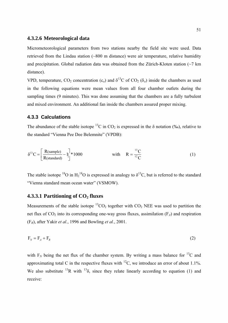
51
2 a
m all four chamber outlets during the
utes). This was done assuming that the chambers are a fully turbulent
and mixed environment. An additional fan inside the chambers assured proper mixing.
nite” (VPDB):
4.3.2.6 Meteorological data
Micrometeorological parameters from two stations nearby the field site were used. Data
retrieved from the Lindau station (~800 m distance) were air temperature, relative humidity
and precipitation. Global radiation data was obtained from the Zürich-Kloten station (~7 km
distance).
VPD, temperature, CO2 concentration (ca) and δ13C of CO (δ ) inside the chambers as used
in the following equations were mean values fro
sampling times (9 min
4.3.3 Calculations
The abundance of the stable isotope 13C in CO2 is expressed in the δ notation (‰), relative to
the standard “Vienna Pee Dee Belem
12
1313
CCR with 1000* 1
RRCδ
(standard)
(sample)=⎥
⎦
⎤⎢⎣
⎡−= (1)
The stable isotope 18O in H218O is expressed in analogy to δ13C, but is referred to the standard
“Vienna standard mean ocean water” (VSMOW).
C and
We also substitute R with δ, since they relate linearly according to equation (1) and
receive:
4.3.3.1 Partitioning of CO2 fluxes
Measurements of the stable isotope 13CO2 together with CO2 NEE was used to partition the
net flux of CO2 into its corresponding one-way gross fluxes, assimilation (FA) and respiration
(FR), after Yakir et al., 1996 and Bowling et al., 2001.
FF F RAN += (2)
with FN being the net flux of the chamber system. By writing a mass balance for 13
12approximating total C in the respective fluxes with C, we introduce an error of about 1.1%. 13 13

52
(3)
nature of the respiration flux, which is comprised of soil and plant respiration. For
eeling
plots (Ogee et al., 2004), which give an integrated value for δN.
the photosynthetic CO2 flux, δA is not easily measured, but can be
canopyaA ∆−= (4)
with δa as the isotopic composition of background CO2 (taking the means from the chamber
utlets, representing the “ambient” air in the canopy; see above) and ∆canopy as the
ters.
onsidered the canopy as a “big leaf” (Ogee et al.,
2003) and the values for the parame articular to calculate
∆canopy is not only the
ination of the plant canopy against C but the discrimination of the whole system;
thus including soil derived 13
discrimination ∆system but reverted to the common name ∆canopy. In analogy to a leaf, the soil
was regarded as an additional mitochondrial CO source within the “big leaf”
al CO
2
mbining equations (2), (3) and (4) we get the
ilation flux FA:
δFδF δF RRAANN +=
with the subscripts of δ corresponding to “net flux” (N), “assimilation” (A) and “respiration”
(R) respectively. FNδN is called isoflux and is the total net 13C flux within the system. δR is the
isotopic sig
an estimate of δR a two-component mixing model is applied on nighttime data (Keeling plot,
after Keeling, 1958). This is the most promising method to assess the isotopic signal of the
daytime respiration flux, with the assumption that isotopic signal of day and nighttime
respiration do not differ substantially (Pataki et al., 2003). δN is derived from daytime K
The isotopic signature of
calculated using the following equation after Bowling et al., 2001:
δ δ
o
photosynthetic 13C discrimination of the canopy. We calculated ∆canopy as shown below, from
transpiration data and micrometeorological parame
It should be noted at this point that we c
ters were chosen accordingly, in p
∆canopy. In the context of this study the term ∆canopy -as commonly found in literature- was used
to signify discrimination against 13C. However in our case 13discrim
C. For better understanding we refrained from naming the system
derived CO2 2
model. The same consideration was applied further below concerning ci (leaf intern 2
concentration) and leaf conductance gc (for H2O and CO2). These two terms were also used
with their common names and should be understood as “big leaf” internal CO concentration
and “big leaf” conductance, as stated above. Co
following equation for the assim

53
δδ ⎥⎦⎢⎣ ∆−− canopyRa
NA
and substituting ∆
δδF ⎥⎤
⎢⎡ −
= RN (5a) F
canopy according to equation (12) we get
1.6cTVPDNEE
1δδ
δδF F
⎥⎥⎥⎥⎥
⎦
⎤
⎢⎢⎢⎢⎢
⎣
⎡
⎥⎦
⎤⎢⎣
⎡××
×−−−−
−=
aRa
RNNA
(b-a)a (5b)
this is in analogy to Yakir et al., 1996 but with the calculation of ∆canopy included. The
spiration flux FR: can then easily be calculated from equation (2).
.3.3.2 Partitioning of water vapor into evaporation and transpiration
re
4
By approximating H2O ≈ 1H216O the mass balance for 18O in the evapotranspiration flux can
be written as:
OH 162
1EETTETET
with the subscripts ET indicating evapotranspiration, T transpiration and E evaporation
respectively. The isotopic ratio R relates linearly to δ
OH 182
1
(6) R RFRF RF with =+=
18O (equation 1) and by substituting FE
with (FET – FT) equation (6) can be rewritten as:
100 δδδδ(%)T ×
−−
=ET
EET with 100F
FT(%) ×=
ET
T (7)
R18O in water vapor from soil evaporation was calculated using soil water Rsoil18O values
from 0-3 cm depth (n=14). Evaporated water is depleted in heavy isotopes relative to the
remaining water body. Evaporated soil water Re18O is a function of the isotopic composition
of vapor in the atmosphere (Ra), the relative humidity (h, expressed as fraction) and

54
quilibrium and kinetic fractionation factors (α* and αk respectively). After Gat, 1996 and
Moreira et al., 1997 we write:
e
k-h α1asoil
ehα 1 R)/(R * −
= (8)
with Re being the R18O of evaporated water and Rsoil the R18O value of soil water. The
fractionation factors α* and αk were inserted as 1.0104 (15°C, average measured soil
temperature, Majoube, 1971) and 1.0189 for a
Ehleringer, 1991). Re was converted to δe using equation (1). It should be noted at this point,
at equation (8) is very sensitive to changes in αk, the kinetic fractionation factor. We
within the well ventilated
chambers. The influence of the relative humidity of air (h) on the fractionation is minor up to
finite
alculated with h=0 by 0.3‰, indicating that relative humidity had only a minor
fluence on fractionation during evaporation.
Assuming steady-state leaf water enrichment, the transpired water vapor isotope signal equals
the source water signal, according to (Wang et al., 2000). For
anspiration (δT), soil water δ18O from 3-12 cm depth was used since this was the depth were
rent research and therefore the values of (δT)
re not firmly established for this study (see discussion). We therefore applied a second
approach where we included leaf water δ18O, which was enriched during the day up to values
of 16.4‰. Since vapo at the site of evaporation within the
aves, equation (8) cannot be applied and the influence of the kinetic fractionation factor αk
fr
R
turbulent boundary layer (Flanagan &
th
decided to use the fractionation factor for a turbulent boundary layer, since at the soil surface,
despite the dense plant canopy, we presumed turbulent conditions
a relative humidity of 0.7 (1‰ change for h=0.7, as compared to h=0) and increases to in
values for h→1. Humidity in our case was h=0.43 as a highest value; this deviates from the
fractionation c
in
δ18O in water vapor from
tr
L. perenne derived its source water from. This was separately assessed by stem water
measurements, which were compared to soil water in different depths (data not shown). Leaf
water isotopic steady state (ISS) is a topic of cur
a
r pressure is around saturation
le
(Cappa et al., 2003) is negligible. We used a simple model with an equilibrium actionation
factor (α*) of 1.0093 for temperatures at 25°C (Majoube, 1971), which was the average
temperature during the afternoons of the samplings:

55
R
R *αleaf
T = (8b)
with RT the R18O of transpired water from 18
water δ18O was determined hourly from 11.00 to 17.00 hours (the water vapor sampling time)
nd the calculated means from each day were inserted in equation (8b).
4.3.3.3 Calculating canopy discrimination
the leaf, Rleaf as the R O value of leaf water. Leaf
a
For the value of δET, the isotopic signal of evapotranspiration, the intercept with the ordinate
of Keeling plots from air water vapor data was used (see below for explanation of Keeling
plots).
According to Farquhar et al., 1989 discrimination (∆) of a plant canopy against 13CO2 during
photosynthesis can be expressed by equation (9):
a
icanopy )a(b- a
cc∆ += (9)
with ā (~4.4‰,) as the kinetic fractionation by CO2 diffusing from the canopy air space to the
site of carboxylation (see equation 9a) and b (~27.5‰) the enzymatic fractionation by the
CO2-fixing enzyme ribulose-1-5-biphosphate-carboxylase (RUBISCO). The ratio ci / ca is the
ratio of the CO2 concentration in the leaf (“big leaf”) intercellular space and ambient air. In
analogy to the explanatory note above concerning ∆canopy , we refer to ci as the theoretical
value of the entire system (plant canopy and soil). This is similar to the “big leaf” model
where an entire plant canopy is regarded as a single, large leaf (Ogee et al., 2003). The “big
leaf” model itself does not include the CO2 efflux from the soil. When, as in our study,
measurements are made within a whole system, soil derived CO2 is an additional source of
CO2. In our “whole system” model this efflux can be regarded as additional mitochondrial
respiration within the “big leaf”, thus making the link back to the “big leaf” model. The same
principle applies for the stomatal conductance gc.
The kinetic fractionation ā is expressed as follows within the big leaf model (Ogee et al.,
2003):

56
1
11))((
−
−
++
+=
macac
cb
gggggagga a
a1 the
yll, estimated with 0.6 mol m-2 s-1, according to Evans & von Caemmerer, 1996. The
by the following relation of ga to gt and
b
++ macsa gggaTa (9a)
where ab is the fractionation of CO2 diffusing through the laminar boundary layer to the
stomata (2.9‰), a denotes diffusional fractionation from the leaf surface to the substomatal
cavity (4.4‰), as(T) is the fractionation when CO2 enters solution (1.1‰ at 25°C) and
fractionation of dissolved CO2 diffusing through water (0.7‰). The canopy conductance gc
for CO2 is calculated from equation (11, gcCO2) and gm is the conductance for CO2 within the
mesoph
aerodynamic conductance for CO2 (ga) is calculated
g (in m s-1, converted to mmol m-2 s-1 with a conversion factor of 37.5 after Nobel, 1983):
bta ggg111
+= (9b)
where 1/ga is the sum of a turbulent resistance (1/gt) and a boundary layer resistance (1/gb),
fter Lamaud et al., 1994. Taking medium values for the turbulent and the boundary layer a
resistance, since the chamber system was a turbulent environment, we receive values of 4.4‰
which are insensitive to changes in canopy conductance gc.
The CO2 concentration of ambient air (ca) can easily be measured (the mean concentration at
the outlets of the chambers, see above), but not the intercellular CO2 concentration ci.
However, ci , assuming the system as a “big leaf”, can be derived from equation (10), once the
assimilation rate A (in our case the absolute value of day time NEE) and the stomatal
conductance (gcCO2) are known.
NEEA g
Acc )c-c(gA withtherefore2
2 =−==cCO
aiiacCO (10)
Stomatal conductance (in our case canopy conductance gcCO2) can be derived from equation
rcellular spaces and the ambient air and gcH2O .
(11) describing the transpiration as a function of the vapor pressure difference between the
leaf inte

57
The transpiration rate is calculated from the measured NEE of H O and equation (7) and
relates to stomatal conductance for water gcH2O
2
as follows:
aicCOOcHcCOaiOcH e-e
T6.1g g1.6g )e-e(gT 2222 get wesince and×
=×== (11)
with T the transpiration in µmol m-2 s-1 and gcCO2 the stomatal conductance for CO2. The term
(ei - ea) is the difference of water vapor p ial pressure from the leaf intercellular space to
ambient air. It is assumed that the relative humidity in the leaf intercellular spaces is 100%, e
art
ent
ir temperature. However, the air in our gas exchange chambers was well mixed based on the
high turbulence within the chambers, so that the temperature difference between ambient air
and the leaves
ith the vapor pressure deficit (VPD) of ambient air within the chambers, which is (esat - ea).
ea) with VPD. Equations (9) and
i
can therefore be calculated as the saturation vapor pressure (esat) for a given (leaf)
temperature. Under non-turbulent conditions the leaf temperature is higher than the ambi
a
was presumed to be negligible. This means that (ei - ea) can be approximated
w
Therefore, if the transpiration rate (calculated from equation (7) and multiplied with the NEE
flux for H2O from the chambers /100), the rate of net photosynthesis (NEE flux for CO2 from
the chambers), VPD and ambient CO2 concentration is known, ∆canopy can be calculated by
combining equations (9) (10) and (11) and substituting (ei -
(10) give:
⎥⎥⎥⎥⎤
⎢⎢⎢⎢⎡
−+=
a
cCOa
canopy )a(b- a c
gNEE
c∆ 2 (12a)
⎦⎣
and by substituting gcCO2 with equation (11) and (ei - ea) with VPD we get:
⎥⎦
⎤⎢⎣
⎡××
×−+=
1.6cTVPDNEE
1∆a
canopy )a(b- a (12b)
58
mponent mixing model (Keeling
lot) was applied using geometric mean (GM) regression. Outliers were selected (and
removed) by an iterative method described by Bowling et al., 2002 using linear
from statistics software R (Gnu public license) for residual calculation. Data points with an
bsolute value of the residual larger than twice the residual standard error were removed and
t
ults
4.4.1 NEE and micrometeorology
The beginning of May 2004 was characterized by low temperatures of 5-10 °C maximum and
cumulated precipitation of 53 L m-
from May 10 to May 12 showed increasing temperatures with maxima up to 20 °C, a VPD of
0 to 14 hPa and a global radiation of over 800 W h m-2. After another rain event with 12 L
5 hPa on May 13.
ubsequently, temperature and VPD increased from day to day until reaching peak values of
26 °C and 24 hPa respectively on May 18 (Figure 16a).
All three CO2 sampling days (May 11
1 and 14, see Figure 20) with peak temperatures of 17 to 26 °C and VPD between 11 and 24
hPa. The first two days had similar micrometeorological conditions and contrasted to the third
day. May 11 and May 14 were characterized by peak temperatures between 17 and 20 °C and
4.3.4 Statistical analysis
For δ13CO2 and δH218O16O source determination a two co
P
regression
a
this process was iteratively repeated. This resulted in removal of 10% of the data points (27 of
273) for CO2 and in 8% (3 of 39) for H2O. GM regression was calculated according to Webb
et al., 1981 using an application written by M. Sawada, University of Ottawa. For error
estimation of the intercepts we followed the suggestions by Pataki et al., 2003 and Sokal &
Rohlf, 1995 using the standard error of the intercept from the linear and not the geometric
regression model.
The four treatments (high N and low N with each former high and low CO2 levels from the
FACE experiment) were pooled since no significant differences were observed between
different treatments. Mid day means of H2O and CO2 NEE were analyzed with a Student’s
test, assuming normal distribution of the individual datasets. Night time Keeling plot
intercepts from former high and low CO2 levels were analyzed with a Student’s t test, also
presuming normal distribution of the underlying datasets.
4.4 Res
2 from May 6 to May 9 (Figure 16a). The following days
1
m-2 during the night of May 12, temperature and VPD dropped to 12 °C and
S
, 14 and 18) were mostly sunny (some clouds on May
1

59
May 18, the third sampling day, temperature reached 26 °C VPD between 11 and 14 hPa. On
and VPD was 1.9 times higher than the mean of the other two days. VPD within the chambers
differed even more between the two sets of meteorological conditions (Figure 18).
NEE of CO2 was highest on day two (May 14), where the mid day average from 12.00 to
14.00 hours reached -27.2 µmol m-2 s-1. Concurrently, the smallest night time respiration flux
of 2.8 µmol m-2 s-1 was observed in the night of May 14. The warm and dry day three showed
the smallest day time NEE of -20.4 µmol m-2 s-1, being 78% of the average of the other two
days. Respiration during the following night was highest of all three sampling days and
reached 3.8 µmol m-2 s-1 (Figure 16b).
-40
-30
-20
-10
0
10
Glo
bal R
adia
tion
(Wh
m-2
)
0
200
1200
400
600
800
1000
VP
D (h
Pa)
and
T (°
C)
0
10
20
30
prec
ipita
tion
(mm
)0
2
8a)
4
6
day (May 2004)
6 8 10 12 14 16 18
Global Rad.VPDprecipitationTemp °C
b)
11 14
NE
E C
O2 (
µ mol
m-2
s-1
)
18
Figure 16 a) Micrometeorological data from May 6 to 19 from the Lindau station, except for global radiation
from the Zürich-Kloten station. b) Measured net ecosystem exchange (NEE) for CO2 from the chambers. Time
periods are from 06.00 to 06.00 hours (May 11) and from 09.00 to 06.00 hours (May 14) and from 10.00 to
10.00 hours (May 18).

60
igure 17, a
rning the transpiration δ18O for comparison. The first
one (i) assuming isotopic steady state (ISS) during transpiration and δ18O equaling stem water
and the second one (ii) based on δ18O of leaf water assuming non-ISS during our sampling
times from 11.00 to 17.00 hours (Figure 17, a and b).
The values for δET were close to the signal of pure transpiration using the stem-water model
(i) and therefore high relative amounts of transpiration were calculated: 96.3 ± 4% for May 29
and 99.2 ± 4% for May 30, according to equation (7). The errors were derived by error
propagation from the individual errors in equation (7). With the leaf-water model (ii) we
calculated relative transpirations of 61.7 ± 3% for May 29 and 64.4 ± 3% for May 30. For
both models the relative transpiration on the two days differed only within the calculated
errors of each, giving mean values of 98% (i) and 63% (ii) respectively.
Both models showed a consistent increase in relative amounts of transpiration from May 29 to
30, by 2.9% (i) and 2.7% (ii) respectively. The driving variable for this increase was the rise
in VPD by 9.5 hPa from May 29 to May 30 (Figure 18). The measured ET flux increased by
9% during the two days, this resulted in a calculated increase of the transpiration flux by 12%
(i) and 14% (ii) between the two days, depending on the model used.
Model (i) seems to overestimate the relative amount of transpiration, since on the two days
prior to sampling there was 15 mm of precipitation (Figure 18) and the soil was moist. Model
(ii) seems to provide more realistic results and is therefore used in the following calculations.
The implications of either model are further discussed in the following results.
4.4.2 Water vapor flux partitioning
The isotopic signal of the evapotranspiration (ET) flux δET as derived by the ordinate
intercepts from Keeling plots were -11.0‰ on May 29 and -10.3‰ on May 30 (F
and b). They differed by 0.7‰ between the two days and the associated errors were ±0.5 and
±0.4‰ respectively. Evaporation δ18O as calculated by equation (8) showed a small
difference of 0.2‰ between the two sampling days, which was mainly caused by the 0.3‰
difference in soil water between the two days. The change in relative humidity from 0.43 to
0.37 attenuated this difference to soil water by 0.1‰.
We applied two different models conce

61
-30
-20
-10
0
10
1 / [H2O] (mmol-1 m3)
0.0000 0.0005 0.0010 0.0015 0.0020 0.0025 0.0030 0.0035
δ 18
O (‰
)
Evaporationr ² = 0.89
Transpiration (leaf water)
intercept = -11.0 ± 0.5‰
a)
Transpiration (stem water)
-40
10
1 / [H2O] (mmol-1 m3)
0.0000 0.0005 0.0010 0.0015 0.0020 0.0025 0.0030
δ 18
O (‰
)
-40
-30
-20
-10
0
Evaporationintercept = -10.3 ± 0.4‰r ² = 0.95
b)
Transpiration (stem water)
Transpiration (leaf water)
cluded in the regression and
, and 13°C on
May 29 and rain periods were observed 1-2 days before each sampling day. On May 30
temperature was higher (16°C), causing the observed increase in VPD (Figure 18).
Nevertheless, and not depending on the model used for calculating transpiration, May 29 and
30 showed an increase of 3% in their relative transpiration rate. These were two consecutive
Figure 17 a) and b) Keeling plots of water vapor from May 29 (a) and 30 (b). The intercepts indicate the
isotopic composition of the evapotranspiration flux. White dots are outliers not in
arrows mark the isotopic value of the evaporation flux and transpiration flux (stem water and leaf water model).
May 11 and 14 showed similar meteorological conditions to the H2O sampling day May 29.
Average 24 hour temperatures were between 11 and 12°C on May 11 and 14

62
days without intermediate precipitation and our data shows that the relative amount of
transpiration increased even with a totally increasing NEE of H2O. The increase of the NEE
was therefore caused by the increase of the absolute transpiration rates by 14% (with model
ii), driven by the higher temperature and VPD. This makes the extrapolation of the measured
relative transpiration rate to May 11, 14 and 18 difficult. May 11 had a preceding day with
high temperature and VPD (Figure 16a), just after the rain event. This could mean that soil
evaporation from the precipitation event would already have diminished again. Otherwise,
May 14 was preceded by a day with low temperature and VPD, following the precipitation
event. This has most likely caused the relative evaporation to be still high on May 14 and
most likely comparable to May 29 (and 30). We address this issue further in the following
sections.
In general, model (i), with stem water does not seem to fit well to the meteorological
conditions, since a relative transpiration of 98% is not realistic in a temperate climatic area
shortly after a rain event. We therefore used model (ii), with leaf water in the following
calculations, but considered model (i) results for comparison.
VPD
(hPa
),pr
ecip
itatio
n (m
m)
0
5
10
15
20
25
30
35
Eva
potra
nspi
ratio
n(m
mol
m-2
s-1
)
0
2
4
6
8
Tem
p (°
C)
0
10
20
30
40
50
60VPD (in chambers)Evapotransp.Precipitation (mm)Temp °C
11 14 18 29 30
day (May 2004)
Figure 18 Mid day (12-14 h) vapor pressure deficit (VPD) in the chambers, and evapotranspiration at the five
sampling days in May 2004. Black bars are precipitation in May 2004. Timescale is linear and error bars are the
andard error of the means. st
4.4.3 Canopy discrimination
The mean value of 63% transpiration (from model ii) of the two H2O sampling days was
taken as a basis to calculate the transpiration fluxes, which are one of the terms in equation
(12b) that was used to calculate the canopy discrimination ∆canopy . Implications of using
model (i) or (ii) will be further discussed below.

63
Canopy discrimination was calculated for the three CO2 sampling days May 11, 14 and 18 at
an hourly time resolution from 12.00 to 18.00 hours. Using model (ii) with 63% transpiration,
the calculated values were between 13.6 and 23.8‰. May 11 and 14 were close together and
May 18, the day with dry conditions, showed consistently lower discrimination values. May
11 and 18 showed a gradual increase during the day, but May 14 varied up to 7‰ within two
hours. The instability of May 11 and 14 was be directly related to meteorological conditions,
see Figure 20 and Figure 21 and further below. The average canopy discrimination of the
entire growth period (Figure 19) was calculated to 20.6‰, from mean plant δ13C of -28.6‰
(δplant) and an estimated mean of -8‰ for atmospheric (δatm) CO2. (∆canopy = δatm – δplant).
12 14 16 18
∆ cano
py
10
12
14
16
18
26
May 11May 14May 18
high VPD, May 18
a)
growth period avg.20
22
24
(‰)
12 14 16 18
c a - c
i (p
pmv)
0
150
200
250
50
100
May 11May 14May 18
high VPD, May 18b)
hours) time of day (
Figure 19 a) Canopy discrimination on May 11, 14 and 18 as calculated by equation (12). Dotted line is the
mean ∆canopy of the entire growth period. b) Differences between chamber ambient and canopy-scale intercellular
CO2 concentrations. May 18 was a dry day characterized by a VPD within the chambers 2.5 times higher than
the average of the other two days (averages from 12-14 h).

64
was
lso increasing, but this was only found on the two days with moderate temperatures and
VPD. All three days showed a close correlation to VPD, with an increase in VPD causing
lower leaf internal CO2 concentrations (Figure 21b).
Leaf-internal CO2 concentration (ci) was calculated from equation (9). Again, May 18, as the
dry and warm day, showed a consistent and stable pattern from 12.00 to 18.00 hours, with an
average value which was 195 ppm lower than the average ambient CO2 concentration. On the
other two days the differences were smaller, lying between 95 and 105 ppm on average,
providing a higher availability carbon to the CO2 fixing enzyme RUBISCO. This caused a
higher discrimination, closer to the maximum value of 27.5‰ (equation 9, if ci / ca =1 is
assumed).
A close link between NEE of CO2 and ∆canopy was found on two days, but not for the dry day
May 18 (Figure 20 and Figure 21a). With an increasing NEE flux, canopy discrimination
a
Glo
bal R
adia
tion
(Wh
m-2
)
0
200
400
600
800
1000
1200
1400
NEE
CO
2 (-
1)(µ
mol
m-2
s-1
)
-10
0
10
20
30
∆ cano
py (‰
)10
20
30
40
50
60NEE CO2 *(-1)
Discrimination
May 11 May 14 May 18
Figure 20 Global radiation, NEE of CO2 (black line) and canopy discrimination (dotted line) on May 11, 14 and
18. Arrows point at events diminishing global radiation (clouds) and white bars are times from 12.00 to 18.00
hours.

65
16
18
20
22
24
26
NEE CO2 (µmol m-2 s-1)
-35 -30 -25 -20 -15 -10 -5 0
a)
∆ cano
py (‰
)
May 11May 14May 18
12
14
VPD (hPa)
0 10 20 30 40
c i / c
a
0.3
0.4
0.5
0.6
0.7
0.8
0.9
May 11, 14May 18b)
t [CO2] versus VPD in the chambers on May 11, 14 and 18. White circles are the dry day May 18.
egression: r2 = 0.81.
4.4.3.1 Influence of transpiration on canopy discrimination
As mentioned above, the relative amount of transpiration from evapotranspiration was
calculated using two different approaches, model (i), with stem water and model (ii), with leaf
water δ18O. To see how this affects the calculated ∆canopy we tested several relative
transpiration rates (Figure 22). Two distinct features were found: the closer ∆canopy is to the
Figure 21 a) Delta canopy versus NEE of CO2 on the three sampling days May 11, 14 and 18. White circles
represent May 18 and regression line through the other dates is with r2 = 0.69. b) Ratio of leaf internal [CO2] to
ambien
R
66
maximum value of 27.5‰ the smaller the effect of any change. Second, the magnitude of
change becomes larger with decreasing transpiration rates.
This means, that an accurate quantification of transpiration becomes more important the dryer
the environmental conditions (decrease of ∆canopy with increasing VPD, see Figure 21b).
Otherwise, dry conditions are generally characterized by a low soil evaporation and high
relative transpiration. This attenuates the magnitude of the error since errors get smaller with
a high transpiration. As an example, shifts in transpiration from 63 to 80% caused shifts
between 0.8 and 3% within our dataset, with the largest changes occurring at low ∆canopy
values (calculated with equation 12b). This seems to be a realistic magnitude of possible
changes, since our dataset covers a wide spectrum from 13.6 to 23.8‰ and changes from 63
to 80% could be realistic under field conditions in temp
erate areas.
∆canopy at 63% Transpiration (‰)
∆ca
nopy
at x
x% T
rans
pira
tion
(‰)
12 14 16 18 20 22 24 26
5
10
15
20
25
1:1 line 63% Transp) (40% Transp80% Transp98% Transp, model (i) 40%
98%
80%
63% (1:1)
Figure 22 ∆canopy from all three days calculated at 63% (model ii) versus ∆canopy calculated at different relative
transpiration rates, 98% corresponding to model (i).

67
.00 hours. After nightfall
O2 concentrations were higher by 5.5 ppm at the outlets compared to the inlets and CO2 was
depleted in 13C by -0.3‰ on the average.
4.4.4 CO2 flux partitioning
4.4.4.1 Day – night course of CO2 and δ13C
Chamber inlet and outlet differences directly show the influence of the enclosed vegetation
and soil. During daytime the outlets showed CO2 concentrations up to 40 ppm lower than the
inlets, this at an average flow rate of 6 L s-1. Simultaneously, CO2 was relatively enriched in 13C compared to the inlets, up to a maximum of 2.2‰ (Figure 23). The enclosed grass
ecosystem segment assimilated CO2 and the relative enrichment of 13C in the remaining air
was caused by the 13C discrimination of the photosynthetic process. A midday peak at 12.00
hours could be observed in these characteristics and a transition time towards night with
increased scattering of individual measurements from 17.00 to 20
C
time (hh:mm) 09:00 13:00 17:00 21:00 01:00 05:00
δ 13
C (‰
)
-2
-1
0
1
2
CO
2 (µm
ol m
ol-1
)
-40
-20
0
20
40δ13C CO2
Figure 23 CO2 and δ13C differences from chamber outlets to inlets on May 11. Night time data was standardized
to day time chamber airflow (6 L s-1 average) to enable comparison. Dark bar indicates night time (sunset at
20:30h), error bars are standard error of the means.
68
as 7.3 times higher than respiratory release at night, the
grassland was a strong CO2 sink during our measurement days (see also Figure 16b).
showed that the investigated grassland areas
days varied by 2.4 to 4.7‰ within one sampling
ay, when different sampling times were used for the calculation (Figure 24). One must note
however, that a two-hour period only consisted of twelve data points. Keeling plots from
10.00 to 19.00 hours were based on a large dataset (n = 66, Figure 25a and b) and also showed
the smallest associated error of all analyzed time intervals within a single day. Since the time
period of interest for the flux partitioning is mid day 12.00 to 14.00 hours, Keeling plots from
that time would be the choice to represent this time period. Nevertheless, whole-day Keeling
plots lied within a range of 0.2‰ of mid day Keeling plots and showed a smaller associated
error on the intercepts (0.1 to 0.6‰ smaller) and were therefore chosen to represent mid day
δN (Table 5).
Midday ecosystem CO2 uptake w
Integrated values for a 24 hour period on May 14
assimilated 7.4 times more carbon during the day than they respired in the night (data not
shown). Midday peak values therefore seem to be a good measure for whole day ecosystem
CO2 uptake.
4.4.4.2 Keeling plots
Intercepts of CO2 Keeling plots can differ during the course of a day or night, depending on
the time period chosen and the number of samples as also shown by Knohl et al., 2005. Both
daytime (δN) and nighttime Keeling plot (δR) intercepts are crucial parameters in equation (5b)
to calculate FR and FA.
Daytime intercepts on the three sampling
d

69
-20
-18
-16
10-19 h10-12 h
-22
C (‰
)
-28
-26
-24
δ 13
-32
-3012-14 h15-19 h
May 11 May 14 May 18
Figure 24 Daytime Keeling plot intercepts for different time spans on the three CO2 sampling days in May 2004.
Error bars are the standard error of the intercepts.
Time periods that deviated from the whole day and mid day intercepts were morning and late
afternoon hours. No pattern regarding intercept values could be found for these transition
times. Day one and three showed less negative values during morning hours and more
egative values in late afternoon hours. On May 14 (day two) the opposite was observed. A
common feature though for the transition times on all days was the generally larger standard
error of the intercept (Figure 24).
The sensitivity of the intercept calculation becomes clear when studying the example of
whole day data from May 11, as shown in Figure 25a and b. CO2 concentrations (without
outliers) covered a range of 64 ppm (329 to 393 ppm) and δ13C values a range of 3.3‰
(Figure 25a). The source value of the Keeling plot two-component mixing model is found by
plotting the inverse of the CO2 concentrations against the corresponding δ13C values and
calculating the intercept of a linear regression model with the ordinate. Extrapolating 1/[CO2]
to zero actually means calculating the δ13C value for
n
[ ]nn
2
COlim∞→
(Figure 25b). Since this is a

70
large extrapolation, the robustness of the fit of the linear model to the underlying data is
crucial. In this example, after outlier removal (see statistical analysis), we calculated an r2 of
0.97 (which was the least of all three days, see Table 5) and a probability of p < 0.001 that the
model was wrong.
1/[CO2] (µmol mol-1)
0.0024 0.0026 0.0028 0.0030 0.0032
δ 13
C (‰
)
-9
-8
-7
-6
-5
-4
r2 = 0.97intercept = -26.2 ± 0.4‰n = 66 with 7 outliers
a)
1/[CO2] (µmol mol-1)
0.0000 0.0005 0.0010 0.0015 0.0020 0.0025 0.0030 0.0035
δ 13
C (‰
)
-25
-20
-15
-10
-5
b)
Figure 25 a) Day time Keeling plot with data from 10 - 19 h on May 11. White dots are outliers not included in
the regression. b) shows the same dat but with the abscissa going to zero and the white box on the ordinate
being the standard error of the intercept.
a
71
culated.
ight time Keeling plots varied within 2‰ between the three days (Table 5) and, like the day
time Keeling plots, showed a trend towards less negative values in the time period from May
11 to May 18. The variation although was less than half as within day time Keeling plots
(which varied by 4.6‰). Sample numbers at night were slightly less than half as during day
time, nevertheless the correlations were consistently very robust with r2 = 0.99 for all three
nights and errors of the intercepts lied between 0.5 and 0.7‰.
Table 5 Intercepts of Keeling plots for night (δR, 22.00 to 01.00 hours) and day periods (δN, 10.00 to 19.00
hours). 10% of the data points were identified as outliers and not included in the regression analysis. All
regressions were with p < 0.001.
date δ R (night) /‰ δ N (day) /‰
Errors of the intercepts from H2O and CO2 Keeling plots were in the same range of 0.4 to
0.9‰ (Figure 17, Table 5). The larger scattering of the H2O data points, being expressed as
lower r2 values, was compensated by a much smaller extrapolation when the intercept with
the abscissa was cal
N
May 11 -30.3 ±0.6 (n=24, r2=0.99) -26.2 ±0.4 (n=66, r2=0.97)
May 14 -28.7 ±0.5 (n=24, r2=0.99) -23.8 ±0.9 (n=66, r2=0.99)
May 18 -28.3 ±0.7 (n=30, r2=0.99) -21.6 ±0.7 (n=63, r2=0.99)
Night time Keeling plots were also time sensitive, like day time plots. Particularly the data
from 20.00 to 22.00 hours shifted the intercepts up to several permil. This period was a
transition time from day to night that showed a much larger scatter of the data than the period
from 22.00 to 01.00 hours (Figure 26). Late night samples from 05.00 hours also showed
large scattering and in addition had the highest CO2 concentrations. The confounding time
periods from 20.00 to 22.00 hours and from late night 05.00 hours were therefore excluded
from the calculation of δR, thus we obtained the most stab possible results (see Table 5). le

72
1/[CO2] (µmol mol-1)
0.0021 0.0022 0.0023 0.0024 0.0025 0.0026 0.0027
δ
-8
-7
-12
-11
-10
-9
13 C
(‰)
22-01 h (n=24)20-22 h (n
-13
=18)05 h (n=6)
Figure 26 Nig ot from May ated into time periods from 20.00 to 22.00 (white
b 0 t 5. gression line is from 22.00 to 01.00
data only, dotted regression line is from all time periods. White circles are outliers not included in the
re No tra night.
.4.4.3 Assessment of CO2 fluxes FR and FA
The factors in equation (5a) need to meet two conditions to calculate useful values for the
assimilation flux FA and consequently the respiration flux FR. First, the numerator (δN - δR)
should be larger than the denominator (δa – δR – ∆canopy) to yield a result ≥ 1. If this fails, the
result is an assimilation flux which is smaller than the NEE and consequently a negative
respiration flux. We will refer to this situation as “error (a)”. The second meaningless result
ht time Keeling pl 14. Data separ
oxes), 22.0 o 01.00 (black circles) and 0 00 (white triangles). Solid re
gressions. te the increasing CO2 concen tion during the course of the
4
Equation (5a) followed a day time course mostly influenced by ∆canopy values and to a lesser
extent by δa (max. variation 1.7‰). The numerator and the denominator of equation (5a) were
calculated on an hourly timescale from 12.00 to 18.00 hours on the three CO2 sampling days.
Three different relative transpiration rates were used; 63% from model (ii) the “leaf
evaporation model”, 80% as an intermediate value and 98% from model (i) the “stem water
model” (Figure 27 a, b and c). Also shown is the value of the denominator for the estimated
mean growth period canopy discrimination of 20.6‰.

73
occurs if one of the factors in the fraction becomes negative, resulting in positive calculated
assimilation fluxes. We refer to this situation as “error (z)”, with “z” derived from zero.
All three tested relative transpiration rates showed an error (z) on at least 3 of 21 points of
time (63% transpiration). The maximum was 7 of 21 data points including the all day mean of
May 14 (98% transpiration). Error (a) occurred largely (10 of 21 points of time) at 63%
transpiration, including the all day mean of May 18. The 80% transpiration simulation
showed only two errors (a) and 98% showed none. This was since an increase in transpiration
and thus canopy conductance caused an increase of ∆canopy (see Figure 22).
The time period from 12.00 to 14.00 showed a higher tendency towards an error (a) on all
three days (with May 14 fluctuating strongly), particularly at low transpiration rates of 63% as
from model (ii). Later afternoon hours from 15.00 onwards and mean values generally
fulfilled the requirements of equation (5a) but with increasing relative transpiration the risk of
an error (z) increased, even for mean values. This was caused by the gradual increase of
∆canopy during the afternoon hours (Figure 19a), except for May 14 which showed a very
nor an error (z) on any of the three days but yielded unrealistic high values for FA on May 18,
e dry day (Figure 28a).
irregular pattern resulting in an error (z) also for the 13.00 hour sampling time and at all
transpiration rates.
Values of the denominator with the growth period mean of ∆canopy showed neither an error (a)
th
74
10Transpiration 63%, model (ii)
a)
4
6
8
(‰)
δa - δR- ∆can
δN - δR
δa - δR- ∆can (all day)
δa - δR- ∆can (all season)
-2
0
2
May 11 May 14 May 1812 18 12 18 12 18
-2
0
2
8
May 11 May 14 May 18
n 80%, intermediateTranspiratio
b)
4
6
‰)
(
12 18 12 18 12 18

75 (‰
)
-4
-2
0
2
4
6
8Transpiration 98%, model (i)
c)
May 11 May 14 May 1812 18 12 18 12 18
Fi
t
gure 27 a) b) and c) Numerator and denominator of equation (5a) used for CO2 flux partitioning on an hourly
imescale (12.00 to 18.00 hours) on May 11, 14 and 18. Black symbols are the denominator (δa – δR – ∆canopy),
grey triangles are the daily means of the denominator and white circles are the numerator (δN - δR). Black
diamonds with white dots are the denominator (δa – δR – ∆canopy) calculated from growth period average ∆canopy.
Shaded areas indicate values of zero and below for which equation (5a) becomes meaningless, since positive
values for the assimilation (FA) would result. Ordinates are time of day (hours).
None of the three relative transpiration situations fitted all three days simultaneously, even
when taking daily mean values. The mean ∆canopy of the entire growth period gave values
close to the calculation of ∆canopy with 63% transpiration on two days, but not on the dry May
18. This shows that day to day changes in relative and absolute transpiration and thus canopy
conductance exert an essential influence on canopy discrimination, which in term is reflected
in the 13CO2 signature. Choosing between the three relative transpiration rates, the
independently gathered CO2 isotopic data fits well when using 80% for May 11 and 18 and
the 63% from model (ii) on May 14. This is an arbitrary selection (regar ing the exact ratios)
but shows and confirms the trend regarding meteorological conditions and relative
transpiration as discussed in the first section “water vapor flux partitioning” (see above).
On this (presumed) basis of relative transpiration rates we can calculate FR and FA from the
CO2 isotopic data and the mean ∆canopy values from 12.00 to 18.00 hours (Figure 28a) plus FA
for growth period means of ∆canopy. The calculated values may not be compared between days,
d
76
since the relative amounts of transpiration rates are only estimates. A re-calculation of ∆canopy
(which was calculating using 63% transpiration for all days in Figure 19a) using the above
stated transpiration rates is shown in (Figure 28b), confirming the trend already seen in Figure
19a, with May 18 showing lower discrimination values than the other two days, although
lying closer together after the re-calculation.
day (May 2004)
CO
2 flu
x (µ
mol
m-2
s-1
)
-120
-40
-20
0
20
NEE FA
FR
FA (growth period avg. discr.)
11 14 18
12 14 16 18
∆ca
nopy
(‰)
12
14
16
18
20
24
26b)
22
May 11May 14May 18
high VPD, May 18
time of day (hours)
growth period avg.
Figure 28 a) NEE, FA and FR as calculated by equation (5a) using 80% relative transpiration for May 11 and 18
and 63% for May 14. Grey structured bar is FA calculated with growth period means for ∆canopy. b) Calculated
∆canopy with equation (12b) using the same amounts of relative transpiration (80, 63 and 80%) as in a). Dotted line
is the mean ∆canopy of the entire growth period.

77
se individual fluxes. Both the transpiration and
vaporation fluxes have their origin in soil water, but undergo different intermediate
processes, which alter δ18O composition individually (Wang et al., 2000).
Evaporating water from soil is strongly depleted in the heavy 18O isotope by the evaporation
process itself, according to equation (8). Relative humidity, temperature and δ18O of the liquid
water body influence the magnitude of this depletion. In our case, we found depletions
between -28.8 and -29.3‰. The basic question still remains, at which soil depth water for this
calculation should be sampled. We decided to use δ18O from 0-3 cm soil depth, since a
difference of 5.3‰ to water from deeper layers was observed on May 29, after a period of
warm and dry weather conditions (data not shown).
Water for transpiration is taken up by the roots of the plants and evaporates with unchanged
δ18O composition, assuming isotopic steady state (ISS) in plant leaves (Yakir et al., 2000).
Recent studies have shown that under field conditions there can be substantial deviations from
ISS with a time lag of up to several hours (Farquhar et al., 2005). An isotopic enrichment of
leaf water can be observed during the day (Dongmann et al., 1974, Flanagan & Ehleringer,
1991, Harwood et al., 1999) and in our study we found enrichments of δ18O up to +16.4‰
(data not shown). Using the model where the transpiration flux has the isotopic composition
of stem water (model i), assuming isotopic steady state (ISS) as applied by Yepez et al., 2003
in a semiarid environment, did not yield convincing results in our case. However, since the
leaf water is the direct source of transpiration and shows a diurnal course in δ18O, with high
enrichment during day time hours (which is also seen in the water vapor of the ambient air,
Bantelmann et al., 2005, unpublished data), we tested a different approach. Model (ii) is using
actiona
ult nitude when compared to the few existing studies that
o of 0.65 in a sparse vine crop whereas a
et al., 2004 found T/ET ratios between 0.7 and 0.82 in a
sparse sorghum canopy. Both authors use models such as Shuttleworth-Walace (Shuttleworth
4.5 Discussion
4.5.1 Water vapor flux partitioning
The isotopic approach to partition ecosystem water vapor fluxes into transpiration and
evaporation bases on δ18O differences of the
e
the isotopic composition of leaf water and with the temperature dependent equilibrium
fr tion the isotopic composition of the transpiration flux δT was calculated. The
obtained res s were acceptable in mag
relate T to ET. Sene, 1994 calculated a T/ET rati
more recent study done by Kato
78
Penman-Monteith to calculate T and ET from meteorological
parameters.
-ISS conditions, which is supported by our data.
003 and Moreira et al., 1997. Deviations
& Wallace, 1985) and
For the model (ii) approach we presumed non
We therefore introduced model (ii) to obtain an isotopic value for δT where the actual isotopic
signature of leaf water is taken into account. From the newest literature it is obvious, that this
is the current basis for in-depth discussions as to how δT should be determined.
4.5.1.1 Keeling plots of H2O
Keeling plots of δ18O from the sampled water vapor correlated not as well to the fitted linear
regressions than 13C CO2 data did (Figure 17, Figure 25). This was most likely caused by the
fact that δ18O of water is altered by evaporation and condensation processes along its way to
the atmosphere and that the water vapor sampling itself involves a freezing and a thawing
process and represents an integration over 30 minutes sampling time. Scattering of water
vapor samples was also observed by Yepez et al., 2
from a linear Keeling plot may further be caused by changes in the relative contributions of E
and T to ET during the course of the day. Nevertheless, the errors of the intercepts were in the
same range (0.5‰) as for CO2 data, since the extrapolation to zero was much smaller. In
addition, the errors for δET were smaller than the errors for δT (1.0‰), as derived from the
means of leaf water measurements showing a daytime course, and can therefore be considered
acceptable.
4.5.2 Discrimination
Discrimination during photosynthesis against 13CO2 was calculated as ∆canopy with equation
(12b). The obtained values with 63% transpiration showed two distinct clusters, one with an
average discrimination of 20.6‰ ± 0.7‰ (SE, standard error) for May 11 and May 14, two
days with moderate temperatures and VPD. The second one, on May 18, showed lower
discrimination ranging from 13.6 to 15.8‰ and with a decrease during the course of the day.
May 18 was characterized by warm temperatures above 25°C and high VPD, the lower values
for ∆canopy on this day were caused by the high VPD of 30.2 hPa within the chambers. The dry
air lead to stomatal closure (decrease in stomatal conductance gcCO2), to a lower ci / ca and to a
lower ∆canopy . This was in analogy to the model developed by Farquhar et al., 1989. These
findings were independent of the model used for the underlying transpiration calculation

79
.
the measured
average leaf material δ13C of -28.6‰: ∆average = -8‰ – (-28.6‰) = 20.6‰. The values we
ther lower by 1.8‰ (model ii) or higher by 1.3‰ (model
to environmental conditions of canopy discrimination was found, in particular to
14, which were partly cloudy, we found a day time course
of canopy, which inversely related to global radiation. This shows that mean values of entire
(Figure 19a and Figure 28b), even though the mean values were lower by 3.1‰ at 63%
transpiration
Mean values of the canopy discriminations from all three days were 18.8‰ for model (ii, leaf
water) and 21.9‰ for model (i, stem water). The average δ13C of leaf material was -28.6 ±
0.6‰ in May 2004. An average value for discrimination during the growth period was
calculated, presuming an average ambient δ13CO2 value of -8‰ and taking
calculated with each model were ei
i). Since our calculated daily means did not include morning hours, where discrimination
generally is higher (Baldocchi & Bowling, 2003) than from 12.00 to 18.00 hours, a lower
mean value in respect to the growth period average value is not a contradiction. In addition,
deviations between long-term and instantaneous ∆canopy have been reported before by Lai et
al., 2003 and Flanagan et al., 1996. Warm and dry days are not prevailing for the local
temperate climate, where 725 mm of precipitation and average temperatures of 13.2 °C are
measured between April and October (30 year means, MeteoSchweiz). It is therefore thought
that a calculated average value, (originating from the two days with moderate temperatures
and VPD, May 11 and 14), which is higher than the growth period ∆canopy might not be
representative. These are indications that in fact model (i) using stem water for δT, might not
be applicable under these climatic conditions and favor model (ii).
A close link
VPD (Figure 21b). On May 11 and
∆
sampling periods should be taken when calculating a partitioning of CO2 fluxes, since the
underlying 13CO2 data is generally derived from means of at least several hours.
Combining calculated ∆canopy with CO2 isotopic data for flux partitioning showed, as a basic
conclusion, that day to day variations in the relative amount of transpiration must have
occurred (presuming accuracy of the CO2 data) and results cannot be readily transferred from
one day to the other. A second characteristic as revealed together with the CO2 data set was
that model (i) with stem water did not yield any results considered acceptable (or realistic) for
all three days, since calculated assimilation fluxes would have been either three or more times
higher than CO2 NEE or returned an error (z), see Figure 27, a-c. Model (ii) with leaf water as
calculated on May 29 and 30was basically applicable for May 14. Intermediate values of 80%

80
t variations between different days in relative transpiration may be substantial.
., 20
ase of day time δN was
-fluxes of δN.
transpiration yielded acceptable results for May 11 and 18, this in analogy to the first
conclusion tha
Thus, using the transpiration values calculated for May 29 and 30 on for other days may cause
a considerable error.
In conclusion, establishing and validating a new model to estimate proportional transpiration
fluxes could provide the basis for a useful alternative to calculate ∆canopy. Particularly on eddy-
covariance sites ∆canopy is generally calculated using the “Penman-Monteith” equation, which
does not always yield satisfactory results (Ogee et al., 2003).
4.5.3 Diurnal and inter-diurnal variations of Keeling plot intercepts
Keeling plots of CO2 data were sensitive to the integrative time period used, this both for day
and night time data. As also reported by Knohl et al 05 we found strong diurnal variations
of Keeling plot intercepts. During two of our three daytime courses the intercept values were
becoming more negative towards late afternoon, but on the third day, May 14, the opposite
was observed. May 14 was the day with the lowest VPD and temperature of all three days and
the one with the highest NEE.
Strong inter-diurnal variations were observed within our eight-day sampling period both for
δR and δN (up to 2 and 4.6‰ respectively). We noted an isotopic link between assimilation
and respiration as also found by Knohl et al., 2005. An incre
consistently followed by an increase of δR during the next night. Increases of day time δN
were more distinct than for night time δR on all three sampling days (see Table 5).
The magnitude of change was not the same within day and night time data. This is presumed
to be a result of the different underlying processes that caused these changes. As discussed
above, variations in δN are an expression of proportional changes within the sub
The photosynthetic flux is the most important since it is the dominating factor by magnitude.
4.5.3.1.1 Day time intercepts
Intercepts of daytime Keeling plots (δN) still represent a mix of two gross CO2 fluxes, namely
photosynthesis and day time respiration (which itself again is comprised of several sub-fluxes;
plant metabolic respiration, photorespiration and soil respiration). Considering this, diurnal
fluctuations of δN actually represent changes in the proportions of the respective gross fluxes.
A proportional increase of the photosynthetic CO2 flux over the respiration flux causes less

81
lest night time respiration of all three sampling days. The opposite
Variations in sub-fluxes are also thought to be the cause for night time δR changes. For δR, the
iration
on of root exudates and different plant compounds are known
till poorly
since in a grassland ecosystem responses are expected to be on a shorter time scale than
reading of fresh assimilates within the plants. It
negative values for δN due to the photosynthetic 13C discrimination (Farquhar et al., 1989).
This was the situation on May 14, meaning that the proportional respiration flux was higher
during morning hours than later in the day. This seems feasible since the night following May
14 showed the smal
situation, a diurnal course with more negative δN towards sunset, shows the proportional
increase of the respiration sub-flux during the course of the day, as seen on May 11 and 18.
4.5.3.1.2 Night time intercepts
division into sub-fluxes can be made as follows: i) plant respiration, ii) plant root resp
iii) respiration of soil organic matter (SOM) by heterotrophic microorganisms (see chapter 3
for further details). These respiration sources show differences in their δ13C signatures. Plant
respiration (i) is assumed to stay relatively constant with little or no isotopic fractionation
occurring during respiration (Lin & Ehleringer, 1997, although Duranceau et al., 1999 found
different δ13C values for respiration at different temperatures. Plant root respiration (ii)
includes heterotrophic respirati
to vary in δ13C composition (Ghashghaie et al., 2001). Finally, heterotrophic respiration of
SOM (iii) can change in δ13C, depending on the soil depth from which it mainly originates
(Nadelhoffer et al., 1988 and chapter 3, this study) and by the involved group of
microorganisms and their current physiological state (Boschker & Middelburg, 2002,
Fontaine et al., 2003). The driving variables for the factors ii) and iii) are s
understood and remain an active area of research.
A link of δR to environmental conditions such as VPD has been described by Högberg et al.,
2001 and Bowling et al., 2002 in forest sites, involving time lags of 5-10 days. Our dataset
showed a strong correlation with VPD 3-4 days earlier (data not shown). This seems feasible
within forest systems, due to the faster sp
should be noted however, that our dataset covered only three night time δR values.
4.5.3.1.3 Time slot for night time sampling
Night time δR was calculated from data between 22.00 to 01.00 hours, excluding the period
from 20.00 to 22.00 and 05.00 hours. Even though net photosynthesis was zero after 20.00

82
e
daytime data, which showed a larger scatter during the whole day period due to the day time
25a), the night time data was relatively stable when
ophic root exudate respiration. Finally,
cing plant
photosynthesis. For a further discussion see Pataki et al., 2003.
could not be further compared to each other
hours and nightfall was at 20.30 hours, Keeling plot data from 20.00 to 22.00 hours
confounded δR by yielding more negative results of up to 1.7‰. The same was the case for
the late night data from 05.00 hours, but to a lesser extent. The data from transition times lied
on the two far ends of night time data when producing Keeling plots (Figure 26). Given the
fact that this data also showed a larger scatter than the mid night data from 22.00 to 01.00
hours, their over-proportional influence on the intercept and thus δR becomes clear. Unlike th
course of photosynthesis (Figure
transition times were not included in the mixing model.
Taking the larger scattering of day time data into account we concluded that the best results
for day time Keeling plots are obtained with an all-day sampling strategy, excluding the
transition times of early morning and early evening. In our case this was from 10.00 to 19.00
hours (day light savings time).
4.5.4 CO2 flux partitioning
The δ13C signature of the daytime respiration flux cannot be measured directly. The basic
assumption has to be made that night time δR is representative for day time δR of the
ecosystem. This assumption involves several independent underlying processes. Respiration
of plants during the day possibly has a different δ13C signature than during the night,
depending on the isotopic composition of the respired substrate molecules (Ghashghaie et al.,
2001, Tcherkez et al., 2003). δ13C of soil respiration might differ from night to day due to
substrate changes in plant root and heterotr
heterotrophic respiration of SOM might be subject to change in isotopic composition.
Considering that the main driving factors for heterotrophic soil respiration are soil
temperature and moisture (Wardle et al., 1990), which stay relatively constant within a 24
hour sampling period, changes in δ13C from heterotrophic SOM respiration are not considered
to be a major factor. It was recently shown by Ekblad et al., 2005 that above ground
meteorological conditions are the driving factor for the whole system by influen
The values of FA and FR as shown in Figure 28
since they were calculated based on assumptions made for the relative transpiration flux.
Nevertheless, we could show that short-term changes in meteorological conditions (even
83
ampling day. May 18 proved to be most sensitive to changes
of input values. The most critical parameter in our case was the transpiration flux, since it
t was estimated via water vapor partitioning using H218O
ich showed large afternoon
zero are critical in regard to slight changes of δa and δR, even by fractions of a permil, since
clouds) can cause large fluctuations of ∆canopy, making CO2 flux partitioning difficult, even
when taking daily means (Figure 27). In the same figure, we demonstrated that the calculation
of FA and FR are strongly influenced by ∆canopy, which in our case was again depending on the
accurate calculation of the transpiration flux. See below for a further discussion of the
individual terms influencing the calculation of FA according to equation (5a).
4.5.5 Sensitivity analysis
4.5.5.1 Calculation of ∆canopy
The calculation of ∆canopy with equation (12b) was relatively robust to variations of a single
factor, since no term in equation (12b) was close to zero. But, as an example, a 20% increase
in NEE of H2O, and simultaneously in VPD, caused ∆canopy to increase between 0.3 and 2.0‰,
depending on time of day and s
could not be directly measured bu
with uncertainties regarding the model that should be applied (stem or leaf water, model i and
ii respectively).
When the relative value of 63% transpiration as calculated by model (ii) is changed to 98%,
as calculated by model (i), we observed increases of ∆canopy between 1.3 and 5.0‰. Again,
May 18 was most sensitive to the variations (see Figure 22). The changes in relative
transpiration presented here are massive, but not unrealistic in a temperate environment. The
calculation of ∆canopy is not hypersensitive to changes in input variables, but since substantial
changes in transpiration may occur between different days this remains a crucial parameter.
This is amplified by the uncertainties of the calculation method for the relative transpiration.
4.5.5.2 Calculation of FR and FA
The values we calculated for ∆canopy brought the term (δa - δR - ∆canopy) in equation (5a) to
values between -2.2 and +8.3‰ depending on time of day and the input model used
(transpiration amount). With the exception of May 14, wh
fluctuations due to changing sunlight, the times from 16.00 to 18.00 hours proved most
critical for being close to zero or negative (Figure 27, a-c). Negative values return a “z-type”
error from equation (5a) as discussed previously. Generally, small but positive values close to

84
n the other hand
are indirectly derived values from Keeling plots and are therefore subject to larger
a , in situ measurement of δa).
N R
nd 2.2. Having a strong isotopic disequilibrium of several permil
A (=
a
values (along a Keeling plot line). An increase of ca by 15 ppm and a simultaneous decrease
the Keeling plot line towards the intercept with the
the risk of an error (z) is high. With the input values we used (Figure 28), all terms were well
away from zero and close attention should be directed to this point when calculating the
partitioning of CO2 fluxes with equation (5a).
The δ13C of ambient CO2, δa, is a value that can be directly measured with a high precision
and is therefore not considered to be an important source of error. δR and δN o
uncertainties than δ (but see below
4.5.5.2.1 Varying δN and δR
We varied day time δN and night time δR in equation (5a) as used in the calculation (see
Figure 28a) by the average error of 0.6‰ from the Keeling plot intercepts. We added 0.6‰ to
δN and subtracted 0.6‰ from δR (case 1) or vice versa (case 2) to test the “extreme” positions.
Case (1) caused the assimilation flux FA to change within ± 3%, corresponding to a maximum
change of 1.2 µmol m-2 s-1. Case (2) lead to changes of FA within ± 5%, being the equivalent
of 2.1 µmol m-2 s-1. The calculations were apparently not sensitive to changes in day and night
time Keeling plot intercepts δ and δ since the fraction in equation (5a) was far from 1,
namely between 1.6 a
between the isotopic signature of the assimilation flux δ δa –∆canopy) and the respiration
flux δR is a prerequisite for not being close to 1 in the fraction of equation (5a).
4.5.5.2.2 ca and δa
The values for ca (ambient CO2 concentration) and δa (δ13C of ambient CO ) are
interconnected. Assuming conditions stay constant, an increase in c means more negative δ
2
a
of δa by 1‰, corresponds to a shift on
ordinate by one fourth of the data range covered by the samples. This resulted in differences
for canopy discrimination of 0.4‰ maximum (for May 18, with a low discrimination). The
effects on FA and FR were much more dramatic, since δa is a direct parameter in the
denominator of equation (5a). Assimilation fluxes FA increased by factors between 1.5 and
2.4, with May 14 being most sensitive. With the concurrent change in ∆canopy the highest
proportional decrease in the denominator was caused, since it was the smallest of all three
days.

85
y elaborate in situ measurements.
tration and δ13C of CO2 can
both be measured with a high precision and are not considered a problem as such. Taking
be readily done in the chamber system used in our study by
different (former) CO2 treatments from FACE
between different plots. This seems reasonable, since respiration of FACE-derived
Nevertheless, ca and δa are not considered to be critical parameters as such, since they can be
directly measured with a high precision. But using an arbitrary “standard” value of -8‰ for ca
should be avoided by all means and replaced b
These simple variations of the underlying data show that ca and δa are highly sensitive
parameters and a locally adapted system design has to ensure that the actual “ambient” values
are being measured. This is the critical point, since the concen
samples of “ambient” air could
taking the values from the chamber outputs, assuming proper mixing inside the chambers. At
eddy-covariance flux sites it might prove more difficult to find a representative location for a
mean “ambient” value, since it should be a sample from the “fresh” air masses within the site.
In particular sites with a high canopy (forests) could be challenging for this task.
Having a strong isotopic disequilibrium between the assimilation and the respiration flux at
the sampling site keeps the fraction in equation (5a) far from 1 and makes equation (5a)
robust to slight changes in δN and δR. This is generally given at sites where C3 photosynthetic
pathway plants prevail, but might prove more difficult at sites with dominating or complete
C4 vegetation, since the isotopic disequilibrium between δA and δR is smaller.
4.5.6 Pooling of data
4.5.6.1 Pooling of
The difference of 2‰ in δ13C of soil organic matter (SOM) between the two former FACE
CO levels was thought to have the largest effect on above ground CO during night time due
to the respiratory release of CO partially containing the isotopic signature of SOM (see
above). No significant differences could be observed when calculating Keeling plot intercepts
from each treatment (Student’s t test). There was not even a (non-significant) pattern to be
found. The intercepts from the plots with more negative SOM δ
2 2
2
13C were more negative than
the control plots on two occasions, May 11 and May 14, but not so on May 18. The
underlying data sets for the Keeling plots consisted of twelve data points each, the intercepts
therefore showed rather large associated errors between 0.5 and 2.3‰. With the present
amount of samples it was therefore not possible to detect an effect of the 2‰ difference in
SOM

86
le within air
amples.
assessment of
proportional transpiration fluxes using H2 O could provide a useful alternative to the
which is often used together with the eddy covariance
measurements. According to our study the new model should consider non isotopic steady
richment.
SOM was shown to be only 40% of total soil respiration on these plots (see chapter 3).
Together with the respiratory CO2 release from plants the δ13C signature of SOM is even
more diluted within the total respiratory flux and was therefore not detectab
s
4.5.6.2 Pooling of different nitrogen fertilization levels
Plant canopies which received a high nitrogen (N) fertilization had larger total leaf areas, this
was reflected in lower intercepted photosynthetic active radiation (PAR) at 5 cm above
ground: 2% for high N fertilization and 13% for low N fertilization (with respect to above
canopy PAR). This might have resulted in a higher assimilation rate for the canopies with the
larger leaf area, but is expected to have been at least partially compensated by a higher
respiration rate. NEE of CO2 and H2O showed no significant differences between these
treatments.
4.6 Conclusions
The calculation of ∆canopy remains a crucial point in CO2 flux partitioning studies besides
finding the best Keeling plots. Establishing a more accurate model for the18
Penman-Monteith equation
state conditions occurring during transpiration and account for leaf water δ18O en
A close link between isotopic signature of assimilation and respiration during the following
night was found, and, in addition, night time δR correlated to meteorological conditions (VPD)
from 3-4 days backwards, prior to sampling. Night time Keeling plots showed a good stability
when excluding the transition times around sunset and early morning, we suggest to start
night time sampling not before complete darkness and to stop before early morning. A
considerable variation of day time Keeling plot intercepts was observed. The time period from
mid-morning to early evening (10.00 to 19.00 hours in our case) provided the most stable
results and matched well with intercepts from the 12.00 to 14.00 hours period. Whole-day
Keeling plots therefore provide a good means to determine mid-day δN.
Open-flow chamber studies provide a relatively well characterized environment in
comparison to “open” field studies which are much more affected by changes in turbulence,

87
d, showed a strong dependence to isotopic values of “ambient” CO2. Locations for
sampling of ambient CO should therefore be carefully chosen when designing sampling
low if a strong isotopic
C01.0056), Federal office for education and Science. Meteorological data with
anks from Agrometeo Switzerland and MeteoSchweiz.
wind direction etc. Nevertheless, the partitioning approaches applied here to a chamber study
are not very stable and are shown to be critically dependent on the models used. A sensitivity
analysis where the used parameters to calculate the partitioning of CO2 fluxes into FA and FR
were varie
2
strategies. Sensitivity to changes in δN and δR was found to be
disequilibrium of several permil between the isotopic signature of the assimilation flux δA
(=δa –∆canopy) and the respiration flux δR is present.
4.7 Acknowledgements
This study is supported by the COST 627 initiative “Carbon storage in European Grasslands”
(Grant No.
th

88
s the open question concerning carbon
equestration and turnover under elevated CO2 could be made.
mpling
odel (Keeling plot, Keeling, 1958)
sed to determine net source values of the air within the investigated area. How high this
recision must be has not been defined yet, but in general, values < 1‰ would seem
acceptable. Pataki et al., 2003 found mean standard errors of the source values of 1.2‰ by
analyzing data from 146 Keeling plots. She also pointed out that the range of sampled CO2
concentrations can be more important than the amount of samples and should be 75 ppm or
larger. This is generally achieved only by sampling over several hours, this applies both for
day and night time.
The computer controlled, automated air sampler (ASA) developed in our study allows for 33
air samples being taken in a programmed sequence. Subsequent analysis in the laboratory is
fast and does not require additional handling of the samples. The ASA is computer-controlled
also during analysis, like an autosampler. Analysis of 33 samples at a continuous-flow mass
spectrometer takes less than six hours and the ASA is ready for the next sampling as soon as
the analysis is finished. The achieved precision was shown to be twice as high as with manual
single-flask analysis, 0.03‰ for δ13C and 0.02‰ for δ18O of CO2 (standard errors SE, n=11).
The ASA is also a useful tool for sampling and analysis of trace gases with concentrations up
to 1000 times smaller than that of CO2; e.g. CO and CH4. Potentially it may also be used for
non-carbon containing trace gases such as nitrous or sulphurous oxides, depending on the
preparation peripherals at the mass spectrometer. The ASA has also been successfully used at
the “High Altitude Research Station Jungfraujoch” and other locations in the Swiss Alps to
5 General Discussion This study advances the field of ecosystem research with stable isotopes by contributing a
novel tool for the automated collection of trace gas samples. Furthermore, a new calculation
approach for the partitioning of net ecosystem fluxes of H2O and CO2 was tested and the
associated uncertainties were broadly discussed. The application of the stable isotope 13C as a
valuable system tracer was demonstrated with the results obtained from SOM within the
former FACE site, where a contribution toward
s
5.1 A novel tool for air sa
Studies on ecosystem CO2 flux partitioning depend on a high frequency, high accuracy and
large enough range of [CO2] and δ13CO2 measurements. This is needed to achieve a high
precision when applying the two-component mixing m
u
p
89
sample CO (unpublished data). Two current projects study the influence of wood burning in a
d the emissions of traffic in a large city, such as Basel.
otranspiration was partitioned
and only in dryer climatic regions than in the current study (e.g. Yepez et al., 2003, Williams
ssumes isotopic steady state (ISS) of transpired
er vapor pressure deficit (VPD) and net carbon assimilation. Still, the new
remote area in southern Switzerland an
5.2 CO2 and H2O flux partitioning
Flux partitioning of the net water vapor flux (evapotranspiration, ET) into transpiration (T)
and soil evaporation (E) was done with the goal to further calculate canopy discrimination
(∆canopy) there from. ∆canopy is a crucial parameter when calculating the partitioning of CO2
fluxes. The currently used model to assess the δ18O composition of the T flux did not yield
acceptable results for our data set. Only in a few studies evap
et al., 2004). The current model for δ18O of T a
water and source or xylem water, meaning the transpired water coming from the soil and
flowing through the stem and evaporating from the leaves has the same isotopic composition
despite the processes in between. Nevertheless, numerous studies have shown previously that
leaf water is strongly enriched in δ18O during the course of a day (Flanagan and Bain et al.,
1991, Harwood et al., 1999). The newest literature discusses observed deviations from ISS
(Farquhar et al., 2005) and the need for an adapted model to calculate δ18O of the T flux has
become apparent. Our approach was to include the isotopic enrichment of leaf water to
determine the δ18O of the T flux. The obtained results for the H2O flux partitioning with this
new model were acceptable in their magnitude and yielded results for ∆canopy which showed a
close relation to wat
model has to be further refined by laboratory experiments, but it should provide grounds for
an in-depth discussion.
From our CO2 data we could derive optimal time slots for CO2 sampling campaigns within a
day or a night. The mixing model (Keeling plot) became less accurate when transition times
from day to night and night to day were included in the sampling. Night time ordinate
intercepts were found to deviate up to 1.7‰ when including time periods around and shortly
after sunset. Night time sampling, which is used to find the isotopic composition of the
respiration flux, should commence not before 1-2 hours after sunset at the earliest and stop
well before dawn. Day time sampling was found best when also excluding transition times,
but, since δ13C is subject to much stronger fluctuations during day than night time (due to
photosynthesis), an even time distribution for sampling over the whole day is to be preferred.

90
tion between the magnitude of the daytime net
wing night. These findings may not be directly
ade on grassland, this can not be readily extrapolated to
We found a close link of δ13C signatures between assimilation and respiration of the
following night. Similar findings have also been made with non-isotope methods;
Aeschlimann et al., 2005 found a close interrela
assimilation and the respiration during the follo
compared but nevertheless show that processes during day time determine the processes of
the subsequent night. Isotopic composition of the night time respiration fluxes during our field
campaign showed a link to meteorological conditions (VPD) 3-4 days prior to sampling. This
is a shorter time-lag than other investigators had recently found for forest ecosystems (Ekblad
et al., 2005, Knohl et al., 2005) but reaction times are expected to be much shorter in a
grassland compared to a forest due to the much smaller canopy and therefore smaller shoot-
root distances.
5.3 Carbon sequestration
The question if grassland soils would be a sink for carbon under elevated CO2 conditions
cannot be answered conclusively since no significant change of the size of the soil carbon
pool was found after ten years of FACE. Studies conducted four and six years prior to this
study came to the same conclusion (Van Kessel et al., 2000). Aeschlimann et al., 2005 found
a long-term stimulation of net CO2 assimilation under elevated CO2 after nine years of FACE,
but this increase was compensated for by a concurrent stimulation of night time respiration.
Net ecosystem carbon input was therefore not significantly increased. These findings do not
support the theory that the soil is the “missing sink” for the amount of the carbon which is
“missing” in the atmosphere (in relation to emission calculations). Since the fore mentioned
studies, including our own, were all m
the entire terrestrial biome. But it raises the question if the magnitude of the calculated fluxes
between biomes, that lead to the “missing sink” theory, is in fact correct. Since the rates of the
individual fluxes within the global carbon cycle are subject to uncertainties, small errors could
propagate and lead to erroneous estimates. Otherwise, the soil is a very heterogeneous system
with a generally large “patchiness” regarding the distribution of compounds. This generally
increases the uncertainties when calculating flux rates. And not to forget, the term “not
significant” does not mean “not happening”; changes could be so small in magnitude that they
are not detectable due to an unfavorable signal to noise ratio.

91
fumigated soils showing a strong 13C label of SOM were in isotopic
plants fixing “normal” undepleted atmospheric CO2
after the fumigation was stopped. This allowed a separation based on the isotopic composition
rsion of a leaf water enrichment
model for H218O should be included (Cernusak et al., 2002). In a next step the back diffusion
5.4 13C as a system tracer
The 13C label within the soil organic matter (SOM), originating from CO2 of fossil origin used
in the FACE experiment, offered a unique opportunity to study SOM-related processes. A
strong label of SOM in 0-12 cm depth (3.4‰) was found after ten years of fumigation with 13C depleted CO2, which decreased by 50% within 960 days after the end of the fumigation
according to our calculations. From this rapidly diminishing isotopic signal we could further
estimate the annual carbon input to be 9.8 ± 3.7 Mg ha-1 which was slightly higher than the
findings of Aeschlimann et al., 2005 and Van Kessel et al., 2000 (both 6.3 Mg ha-1), but the
studies did only calculate the input for 0-10 cm soil depth and not for 0-12 cm as we did.
Furthermore, the associated errors were large (> 1/3 of the actual value) in all studies.
The formerly
disequilibrium with the newly grown
of soil CO2 of respired carbon derived from labeled SOM and from fresh plant material.
Rhizosphere respiration was thus calculated to account for 61% of total soil respiration.
Again, as outlined above that night time respiration is driven by recent assimilation, this
shows that ecophysiological factors driving plant activity are of considerable importance for
below-ground processes.
5.5 Outlook
New advances for gathering 13CO2 data from field sites have recently been made. Schnyder et
al., 2004 introduced a setup for high frequency in situ on-line measurements with a mass
spectrometer. Bowling and Sargent et al., 2003 tested tunable diode laser (TDL) technique for
high frequency analysis of 13CO2 based on the specific absorption of 13C in the infrared
spectrum. This seems to be a promising method if the associated technical effort can be
reduced (need for liquid nitrogen, N2(l)), and the precision increased (0.25‰ currently), in
particular in combination with high-frequency eddy-covariance measurements for net CO2
and H2O ecosystem exchange. Nevertheless, the large amounts of data produced by these
systems would also need to be handled.
The presented model for assessing the H218O signature of the transpiration flux in plant
canopies must be further developed. In a first step the new ve

92
bient air through the stomata into the leaf needs to be
ociated
d promising tool.
of depleted water vapor from the am
considered. For a parametrisation and testing of this new model, laboratory scale gas
exchange chamber measurements and experiments in phytotrons with H218O marked soil
water are needed. Differences in the δ18O enrichment in leaves between species should be
addressed as well as differences in soil evaporation between different soil types (e.g. sandy
soils and loamy soils).
δ18O of CO2 has a large potential to improve the partitioning of carbon fluxes between the
atmosphere and terrestrial ecosystems. The underlying processes leading to the isotopic
signature are well known (18O equilibration between the water body and the CO2 with which
it gets in contact) and the principles understood (Ogee et al., 2004). The current ass
problems evolve from the large scattering of δ18O in these samples. This calls for an increased
effort to improve the sampling methods. Recent attempts to use the δ18O in CO2 as a proxy for
leaf and soil water enrichment are promising (Theis, unpublished data, Bowling, unpublished
data).
In our study the basic applicability of water vapor and CO2 flux partitioning on a temperate
grassland site was demonstrated. There is need for further research in particular regarding the
link of H2O and CO2 partitioning models. The combination of stable oxygen and carbon
isotopes is a very useful an

93
and Environment, in press,
nt, J., Wagner, G. H. & Mariotti, A., 1988. Soil organic matter turnover in long-term field experiments as revealed by carbon-13 natural abundance. Soil Science Society of America Journal, 52, 118-124.
, 294, 2130-2136.
oschker, H. T. S. & Middelburg, J. J., 2002. Stable isotopes and biomarkers in microbial ecology. FEMS Microbiology Ecology, 40, 85-95.
Bowling, D. R., McDowell, N. G., Bond, B. J., Law, B. E. & Ehleringer, J. R., 2002. 13C content of ecosystem respiration is linked to precipitation and vapor pressure deficit. Oecologia, 131, 113-124.
Bowling, D. R., Pataki, D. E. & Ehleringer, J. R., 2003. Critical evaluation of micrometeorological methods for
measuring ecosystem-atmosphere isotopic exchange of CO2. Agricultural and Forest Meteorology, 116, 159-179.
Bowling, D. R., Sargent, S. D., Tanner, B. D. & Ehleringer, J. R., 2003. Tunable diode laser absorption
spectroscopy for stable isotope studies of ecosystem-atmosphere CO2 exchange. Agricultural and Forest Meteorology, 118, 1-19.
Bowling, D. R., Tans, P. P. & Monson, R. K., 2001. Partitioning net ecosystem carbon exchange with isotopic
fluxes of CO2. Global Change Biology, 7, 127-145. Broecker, W. S. & Peng, T. H., 1992. Interhemispheric transport of carbon dioxide by ocean circulation. Nature,
356, 587-589. Buchmann, N., 2000. Biotic and abiotic factors controlling soil respiration rates in Picea abies stands. Soil Biol.
Biochem., 32, 1625-1635. Bundt, M., Jäggi, M., Blaser, P., Siegwolf, R. T. W. & Hagedorn, F., 2001. Carbon and Nitrogen Dynamics in
Preferential Flow Paths and Matrix of a Forest Soil. Soil Science Society of America Journal, 65, 1529-1538.
6 References Aeschlimann, U., 2003. Effects of elevated atmospheric pCO2 on net ecosystem CO2 exchange in managed
grassland. Thesis, ETH Zurich, 15182, Aeschlimann, U., Nösberger, J., Edwards, P. J., Schneider, M. K., Richter, M. et al., 2005. Responses of net
ecosystem CO2 exchange in managed grassland to long-term CO2 enrichment, N fertilization and plant species. Plant, Cell
Amundson, R., Stern, L., Baisden, T. & Wang, Y., 1998. The isotopic composition of soil and soil-respired CO2.
Geoderma, 82, 83-114. Baldocchi, D. D. & Bowling, D. R., 2003. Modelling the discrimination of 13CO2 above and within a temperate
broad-leaved forest canopy on hourly to seasonal time scales. Plant, Cell and Environment, 26, 231-244.
Baldocchi, D. D., Hicks, B. & Meyers, T., 1988. Measuring biosphere atmosphere exchanges of biologically
related gases with micrometeorological methods. Ecology, 69, 1331-1340. Balesdent, J. & Mariotti, A., 1987. Natural 13C abundance as a tracer for studies of soil organic matter
dynamics. Soil Biol. Biochem., 10, 25-30. Balesde
Beer, J., Mende, W. & Stellmacher, R., 2000. The role of the sun in climate forcing. Quaternary Science
Reviews, 19, 403-415. Bond, G., Kromer, B., Beer, J., Muscheler, R., Evans, M. N. et al., 2001. Persistent solar influence on north
Atlantic climate during the Holocene. Science B

94
., DePaolo, D. J. & Cohen, R. C., 2003. Isotopic fractionation of water during ophysical Research-Atmospheres, 108, 4525 doi:10.1029/2003JD003597.
ter lius under field conditions. Plant, Cell and Environment,
Craig, H.n Stable Isotopes in Oceanographic Studies and
Graa ., Six, J., Harris, D., Blum, H. & Van Kessel, C., 2004. Decomposition of soil and plant carbon
he
d by ather conditions. Oecologia, 143, 136-142.
f 127, 305-308.
9-
of leaf
n ., Berry, S. C. & Ehleringer, J. R., 1996. Carbon isotope discrimination
Cappa, C. D., Hendricks, M. Bevaporation. Journal of Ge
Cernusak, L. A., Pate, J. S. & Farquhar, G. D., 2002. Diurnal variation in the stable isotope composition of wa
and dry matter in fruiting Lupinus angustifo25, 893-907.
& Gordon, L., 1965. Deuterium and Oxygen-18 variations in the ocean and marine atmosphere. In: Tongiorgi, E., (ed), Proceeding of a Conference oPaleotemperatures, Laboratory of Geology and Nuclear Science, Spoleto, Italy. Lischi and Figli, Pisa, 9-130.
Craine, J. M., Wedin, D. A. & Chapin, F. S., 1999. Predominance of ecophysiological controls on soil CO2 flux
in a Minnesota grassland. Plant and Soil, 207, 77-86.
f, M.-ADe from pasture systems after 9 years of exposure to elevated CO2: impact on C cycling and modeling. Global Change Biology, 10, 1922-1935.
Dongmann, G., Nurnberg, H. W., Forstel, H. & Wagener, K., 1974. On the Enrichment of H2(18-O) in t
Leaves of Transpiring Plants. Radiation and Environmental Biophysics, 11, 41-52. Duranceau, M., Ghashghaie, J., Badeck, F., Deleens, E. & Cornic, G., 1999. delta C-13 of CO2 respired in the
dark in relation to delta C- 13 of leaf carbohydrates in Phaseolus vulgaris L-under progressive drought. Plant Cell and Environment, 22, 515-523.
Ekblad, A., Boström, B., Holm, A. & Comstedt, D., 2005. Forest soil respiration rate and d13C is regulate
recent above ground we Ekblad, A. & Högberg, P., 2001. Natural abundance of 13C in CO2 respired from forest soils reveals speed o
link between tree photosynthesis and root respiration. Oecologia, Evans, J. R. & von Caemmerer, S., 1996. Carbon dioxide diffusion inside leaves. Plant Physiology, 110, 33
346. Farquhar, G. D. & Cernusak, L. A., 2005. On the isotopic composition of leaf water in the non-steady state.
Functional Plant Biology, 32, 293-303. Farquhar, G. D., Ehleringer, J. R. & Hubick, K. T., 1989. Carbon Isotope Discrimination and Photosynthesis.
Annual Review of Plant Physiology and Plant Molecular Biology, 40, 503-537. Flanagan, L. B., Bain, J. F. & Ehleringer, J. R., 1991. Stable oxygen and hydrogen isotope composition
water in C3 and C4 plant species under field conditions. Oecologia, 88, 394-400.
, L. B., Brooks, R., Varney, G. TFlanagaduring photosynthesis and the isotope ratio of respired CO2 in boreal forest ecosystems. Global Biogeochemical Cycles, 10, 629-640.
Flanagan, L. B. & Ehleringer, J. R., 1991. Stable isotope composition of stem and leaf water: applications to the
study of plant water use. Functional Ecology, 5, 270-277. Fontaine, S., Mariotti, A. & Abbadie, L., 2003. The priming effect of organic matter: a question of microbial
competition? Soil Biology and Biochemistry, 35, 837-843. Friedli, H., Lötscher, H., Oeschger, H., Siegenthaler, U. & Stauffer, B., 1986. Ice core record of the 13C/12C
ratios of atmospheric CO2 in the past two centuries. Nature, 324, 237-238.

95 at, J. R., 1996. OXYGEN AND HYDROGEN ISOTOPES IN THE HYDROLOGIC CYCLE. Annu. Rev.
hashghaie, J., Duranceau, M., Badeck, F. W., Cornic, G., Adeline, M. T. et al., 2001. delta C-13 of CO2
ifford, R. M., 1994. The global carbon cycle: a viewpoint on the missing sink. Australian Journal of Plant
Harwoo
pour within a Quercus petraea forest canopy. Oecologia, 119, 109-119.
-species mixture to free air CO2 enrichment and management. Global Change Biology, 3, 149-160.
Hendrey l
g
ungate, B. A., Holland, E. A., Jackson, R. B., Chapin, F. S., Mooney, H. A. et al., 1997. The fate of carbon in
nes, M. B. & Donnelly, A., 2004. Carbon sequestration in temperate grassland ecosystems and the influence of
ato, T., Kimura, R. & Kamichika, M., 2004. Estimation of evapotranspiration, transpiration ratio and water-use
3-
s. 22-334.
t. Oecologia, 142, 70-82.
Lai, C. T ampling in a tallgrass prairie to partition net ecosystem CO2 exchange. Journal of Geophysical Research-Atmospheres, 108,
Lamaudrosol particles above a pine forest. Journal of Geophysical
Research-Atmospheres, 99, 16511-16521.
Lin, G. H oes not occur during dark respiration in C-3 and C-4. Plant Physiology, 114, 391-394.
Maier-R ean uptake of CO2: interaction between ocean circulation and biology. Climate Dynamics, 711-721.
Majoube apeur. J. de Chim. Phys. et de Phys.-Chim. Biol, 68, 1423-1436.
GEarth Planet. Sci., 24, 225-262.
Grespired in the dark in relation to delta C- 13 of leaf metabolites: comparison between Nicotiana sylvestris and Helianthus annuus under drought. Plant Cell and Environment, 24, 505-515.
GPhysiology, 21, 1-15.
d, K. G., Gillon, J. S., Roberts, A. & Griffiths, H., 1999. Determinants of isotopic coupling of CO2 and water va
Hebeisen, T., Lüscher, A., Zanetti, S., Fischer, B. U., Hartwig, U. A. et al., 1997. Growth response of Trifolium
repens L. and Lolium perenne L. as monocultures and bi
, G. R., 1992. Global greenhouse studies: need for a new approach to ecosystem management. CriticaReviews in Plant Sciences, 11, 61-74.
Högberg, P., Nordgren, A., Buchmann, N., Taylor, A. F. S., Ekblad, A. et al., 2001. Large-scale forest girdlin
shows that current photosynthesis drives soil respiration. Nature, 411, 789-792. Houghton, J. T., Ding, Y., Griggs, D. J., Noguer, M., van der Linden, P. J. et al., 2001. Climate Change 2001:
The Scientific Basis. Cambridge University Press, Cambridge, 183–237.
Hgrasslands under carbon dioxide enrichment. Nature, 388, 576-579.
Jomanagement, climate and elevated CO2. New Phytologist, 164, 423-439.
Kefficiency from a sparse canopy using a compartment model. Agricultural water management, 65, 17191.
Keeling, C. D., 1958. The concentration and isotopic abundances of atmospheric carbon dioxide in rural area
Geochimica et Cosmochimica Acta, 13, 3 Knohl, A., Werner, R. A., Brand, W. A. & Buchmann, N., 2005. Short-term variations in d13C of ecosystem
respiration reveals link between assimilation and respiration in a deciduous fores
., Schauer, A. J., Owensby, C., Ham, J. M. & Ehleringer, J. R., 2003. Isotopic air s
, E., Brunet, Y., Labatut, A., Lopez, A., Fontan, J. et al., 1994. The Landes experiment: Biosphere-atmosphere exchanges of ozone and ae
. & Ehleringer, J. R., 1997. Carbon isotopic fractionation d
eimer, E., Mikolajewicz, U. & Winguth, A., 1996. Future oc
, M., 1971. Fractionnement en oxygène 18 et en deutérium entre l'eau et sa v

96 a
ss spectrometry. Analytical Chemistry, 70, 5159-5161.
pe
n st ambient vapour based on isotopic measurements. Global Change Biol, 3, 439-
450.
Mortaza CO2 and d18O-CO2 ratios at ambient CO2 concentrations for biological applications and the influence of container type and
adelhoffer, K. J. & Fry, B., 1988. Controls on Natural Nitrogen-15 and Carbon-13 Abundances in Forest Soil
elson, S. T., 2000. Sample vial influences on the accuracy and precision of carbon and oxygen isotope ratio
ditions. Global Change Biology, 3, 411-416.
Nobel, P n, New York, 393.
roductivity. CAB International, Wallingford, Oxon, pp. 271–291.
Ogee, J. similation and respiration using (CO2)-C-13 measurements: A cost-effective sampling strategy.
Global Biogeochemical Cycles, 17, art. no.-1070.
Ogee, J. 04. Partitioning net ecosystem carbon exchange into net assimilation and respiration with canopy-scale isotopic measurements: An error propagation
9. O'Leary ., 1981. Carbon isotope fractionation in plants. Phytochemistry, 20, 553-567.
1022.
Pearcy, d ll, London,
lysis. Biol Fertil Soils, 41, 153-162.
of Nature, 399, 429-436.
Mak, J. E. & Yang, W., 1998. Technique for analysis of air samples for 13C and 18O in carbon monoxide vicontinuous-flow isotope ratio ma
McNamara, N., Benham, D., Sleep, D., Grant, H. & Stott, A., 2002. Development of a trace gas stable isoto
capture system in a mobile laboratory for temporal and spatial sampling of field and laboratory experiments. Rapid Communications in Mass Spectrometry, 16, 2165-2171.
Moreira, M. Z., Sternberg, L. D. L., Martinelli, L. A., Victoria, R. L., Barbosa, E. M. et al., 1997. Contributio
of transpiration to fore
vi, B. & Chanton, J. P., 2002. A rapid and precise technique for measuring d13C-
storage time on the sample isotope ratios. Rapid Communications in Mass Spectrometry, 16, 1398-1403.
NOrganic Matter. Soil Science Society of America Journal, 52, 1633-1640.
Nanalysis in continuous flow mass spectrometric applications. Rapid Communications in Mass Spectrometry, 14, 293-297.
Nitschelm, J. J., Lüscher, A., Hartwig, U. A. & Van Kessel, C., 1997. Using stable isotopes to determine soil
carbon input differences under ambient and elevated atmospheric CO2 con
. S., 1983. Biophysical Plant Physiology and Ecology. W. H. Freema
Nösberger, J., Blum, H. & Fuhrer, J., 2000. Crop ecosystem responses to climatic change: productive grasslands.
In: Reddy, K.R., Hodges, H.F. (eds.), Climate Change and Global Crop P
, Peylin, P., Ciais, P., Bariac, T., Brunet, Y. et al., 2003. Partitioning net ecosystem carbon exchange intonet as
, Peylin, P., Cuntz, M., Bariac, T., Brunet, Y. et al., 20
analysis with (CO2)-C-13 and (COO)-O-18 data. Global Biogeochemical Cycles, 18, art. no.-GB201
, M. H Pataki, D. E., Ehleringer, J. R., Flanagan, L. B., Yakir, D., Bowling, D. R. et al., 2003. The application and
interpretation of Keeling plots in terrestrial carbon cycle research. Global Biogeochemical Cycles, 17,
R. W., Ehleringer, J. R., Mooney, H. A. & Rundel, P. W. e., 1989. Plant Physiological Ecology FielMethods and Instrumentation. Chapman and Ha
Pelz, O., Abraham, W.-R., Saurer, M., Siegwolf, R. T. W. & Zeyer, J., 2005. Microbial assimilation of plant-
derived carbon in soil traced by isotope ana Petit, J. R., Jouzel, J., Raynaud, D., Barkov, N. I., Barnola, J.-M. et al., 1999. Climate and atmospheric history
the past 420,000 years from the Vostok ice core, Antarctica. Post, W. M., Emanuel, W. R., Zinke, P. J. & Stangenberger, A. G., 1982. Soil carbon pools and world life zones.
Nature, 298, 156-159.

97
16, 339-345.
118,
chimel, D. S., 1995. Terrestrial ecosystems and the carbon cycle. Global Change Biology, 1, 77-91.
Schneidege
y, 10, 1377-1388.
alysis for Keeling plot applications. Rapid Communications in Mass Spectrometry, 18, 3068-3074 (DOI: 10.1002/rcm.1731).
Sene, K. st
J.
ims, P. L. & Risser, P. G., 2000. Grasslands. In: Barbour M. G., Billings, W. G. (eds) Cambridge University
nt and Soil,
oe, A. R. B., Giesemann, A., Anderson, T. H., Weigel, H. J. & Buchmann, N., 2004. Soil respiration under
okal, R. R. & Rohlf, F. J., 1995. Biometry. W. H. Freeman, New York,
oussana, J. F., Loiseau, P., Vuichard, N., Ceschia, E., Balesdent, J. et al., 2004. Carbon cycling and
Steinma f, R. T. W., Saurer, M. & Körner, C., 2004. Carbon fluxes to the soil in a mature
temperate forest assessed by 13C isotope tracing. Oecologia, 141, 489-501.
Tcherke 3. Metabolic Origin of Carbon Isotope Composition of Leaf Dark-Respired CO2 in French Bean. Plant Physiology, 131, 237-244.
Theis, D. utomated system for trace gas sampling in the field and stable isotope analysis in the laboratory. Rapid Communications in
an Groenigen, K. J., Six, J., Harris, D., Blum, H. & Van Kessel, C., 2003. Soil C-13-N-15 dynamics in an N-2-
Ribas-Carbo, M., Still, C. & Berry, J., 2002. Automated system for simultaneous analysis of d13C, d18O and CO2 concentrations in small air samples. Rapid Communications in Mass Spectrometry,
Schauer, A. J., Lai, C.-T., Bowling, D. R. & Ehleringer, J. R., 2003. An automated sampler for collection of
atmospheric trace gas samples for stable isotope analyses. Agricultural and Forest Meteorology,113-124.
Scheidegger, Y., Saurer, M., Bahn, M. & Siegwolf, R. T. W., 2000. Linking stable oxygen and carbon isotopes
with stomatal conductance and photosynthetic capacity: a conceptual model. Oecologia, 125, 350-357.
S
r, M. K., Lüscher, A., Richter, M., Aeschlimann, U., Hartwig, U. A. et al., 2004. Ten years of free-air CO2 enrichment altered the mobilization of N from soil in Lolium perenne L. swards. Global ChanBiolog
Schnyder, H., Schäufele, R. & Wenzel, R., 2004. Mobile, outdoor continuous-flow isotope-ratio mass
spectrometer system for automated high-frequency 13C- and 18O-CO2 an
J., 1994. Parameterisations for energy transfers from a sparse vine crop. Agricultural and ForeMeteorology, 71, 1-18.
Shuttleworth, W. J. & Wallace, J. S., 1985. Evaporation from sparse crops - an energy combination theory. Q.
R. Meteorol. Soc., 111, 839-855.
SPress, New York, pp 323-356,
Six, J., Carpentier, A., van Kessel, C., Merckx, R., Harris, D. et al., 2001. Impact of elevated CO2 on soil
organic matter dynamics as related to changes in aggregate turnover and residue quality. Pla234, 27-36.
Smith, B. N. & Epstein, S., 1971. Two categories of 13C/12C ratios for higher plants. Plant Physiology, 47, 380-
384.
Selevated CO2 and its partitioning into recently assimilated and older carbon sources. Plant and Soil, 262, 85-94.
S S
sequestration opportunities in temperate grasslands. Soil Use and Management, 20, 219-230.
nn, K., Siegwol
z, G., Nogues, S., Bleton, J., Cornic, G., Badeck, F. et al., 200
E., Saurer, M., Blum, H., Frossard, E. & Siegwolf, R. T. W., 2004. A portable a
Mass Spectrometry, 18, 2106-2112 (DOI: 10.1002/rcm.1596).
Vfixing clover system under long-term exposure to elevated atmospheric CO2. Global Change Biology, 9, 1751-1762.

98 er
ang, X.-F. & Yakir, D., 2000. Using stable isotopes of water in evapotranspiration studies. Hydrological
ardle, D. A. & Parkinson, D., 1990. Interactions between microclimatic variables and the soil microbial
illiams, D. G., Cable, W., Hultine, K., Hoedjes, J. C. B., Yepez, E. A. et al., 2004. Evapotranspiration
ral and
ie, Z., Cadisch, G., Edwards, G., Baggs, E., M. & Blum, H., 2005. Carbon dynamics in a temperate grassland
akir, D. & Sternberg, L. D. L., 2000. The use of stable isotopes to study ecosystem gas exchange. Oecologia,
akir, D. & Wang, X. F., 1996. Fluxes of CO2 and water between terrestrial vegetation and the atmosphere
epez, E. A., Williams, D. G., Scott, R. L. & Lin, G. H., 2003. Partitioning overstory and understory
anetti, S., Hartwig, U. A., Lüscher, A., Hebeisen, T., Frehner, M. et al., 1996. Stimulation of Symbiotic N2
ology, 112, 575-583.
Van Kessel, C., Nitschelm, J., Horwath, W. R., Harris, D., Walley, F. et al., 2000. Carbon-13 input and turn-ovin a pasture soil exposed to long-term elevated atmospheric CO2. Global Change Biology, 6, 123-135.
Wang, W. J., Dalal, R. C., Moody, P. W. & Smith, C. J., 2003. Relationships of soil respiration to microbial
biomass, substrate availability and clay content. Soil Biology and Biochemistry, 35, 273-284.
WProcesses, 14, 1407-1421.
Wbiomass. Biol Fertil Soils, 9, 273-280.
Webb, T., Howe, S. E., Bradshaw, R. H. W. & Heide, K. M., 1981. Estimating plant abundance from pollen
percentages: the use of regression analysis. Review of Palaeobotany and Palynology, 34, 269-300.
Wcomponents determined by stable isotope, sap flow and eddy covariance techniques. AgricultuForest Meteorology, 125, 241-258.
Xsoil after 9 years exposure to elevated CO2 (Swiss FACE). Soil Biol. Biochem., 37, 1387-1395.
Y123, 297-311.
Yestimated from isotope measurements. Nature, 380, 515-517.
Yevapotranspiration in a semiarid savanna woodland from the isotopic composition of water vapor.Agricultural and Forest Meteorology, 119, 53–68.
ZFixation in Trifolium repens L. under Elevated Atmospheric pCO2 in a Grassland Ecosystem. Plant Physi

99
efinition
s and
onds electron cloud around its nucleus, which corresponds
he
econd component of the nucleus are neutrons, with no electric charge. Isotopes are defined as
e
isotop ning “same place”; this refers to the “same place” in the
asic chemical, but rather in physical properties due to their different mass and can be
detected with the appropriate instrumentation, for example a mass spectrometer.
ple 14C, de adiation and are therefore called
are
disting of an element (e.g. C). Abundances of
he
total ca
O + 17O +18O, all stable). Since their mass differs slightly, physical processes like phase
change, diffusion and adsorption lead to accumulation or depletion of stable isotopes within
different compartments in nature. This is referred to as a “fractionation” process.
Mass spectrometry
Isotopes are measured with mass spectrometers, which have a history of almost one hundred
years. Since then, mass spectrometry has been continuously improved in measurement
precision. Since only gaseous compounds can be analyzed directly, solid and liquid samples
need first to be transferred to a gaseous state. For the example of carbon and oxygen, this is
done by either pyrolysis or oxidative combustion. The resulting gases contain the original
carbon or oxygen atoms but now coupled to newly introduced carbon or oxygen atoms, giving
either carbon dioxide (CO2) or carbon monoxide (CO), depending on the atom of interest.
C + O2 CO2 or O + C CO
Appendix A short introduction to stable isotopes and their applications D
The number of protons within an atom determines its basic chemical properties, which for
example, makes a certain atom to be a “carbon” or a “sulfur” atom. Chemical reaction
between atoms take place in the b
to the nucleus in electric charge (with the exceptions of ions, where charges deviate). T
s
atoms with the same number of protons but a different number of neutrons. The nam
e” is derived from Greek, mea“
periodic table of the elements. This means that isotopes of a single element do not differ in
b
There are chemically stable and unstable forms of isotopes. Unstable isotopes, for exam
cay over time and are a source of radioactive r
“radionuclides”. Stable isotopes, in contrast, for example 13C, do not decay and
uishable by mass from the “main” isotope 12
stable isotopes are a percentage fraction or less, for instance 13C accounts for 1.1 % of t
rbon (12C + 13C +14C, the latter is a radionuclide) and 18O for 0.2 % of the total oxygen
(16

100
is ionized in high vacuum by a cathode beam and then accelerated by a
1). The
ffering in mass, are deflected from their flight path proportionally to their mass
The obtained gas
high-voltage electric field (3-5 kV). Focused to a thin ion beam by two parallel plates, the
positively charged ions are deflected in a strong (adjustable) magnetic field (Figure
isotopes, di
and hit the detector at different points. The intensity of the ion beam at each detection point is
then calculated into a ratio for the isotopes. Measurements are always made relative to a
standard gas which needs to be injected with every sample. The obtained ratio is then
expressed relative to an international standard; VPDB for carbon or SMOW for oxygen as an
example.
Figure 1 Schematic of an isotope ratio mass spectrometer
The notation used to express the ratio of a sample relative to a standard is the “δ” which itself
expressed as a ‰ fraction, here shown for 13C: is dimensionless but is
12
1313
CCR with 1000* 1
RRCδ
(standard)
(sample)=⎥
⎦
⎤⎢⎣
⎡−=
Positive values for δ therefore mean a sample is enriched relative to the standard, whereas
zero means equality and negative values indicate depletion. As an example: the standard for 13C (VPDB) contains an absolute amount of 1.1237% of 13C. An air sample of CO2 which
contains 1.1147% 3 of 1 s a δ13 C, therefore ha C value of -8‰.

101
on processes, making rainfall more depleted in 18O the further away it falls from
the evaporating source, which often is the ocean (Figure 2).
Applications
As pointed out above, abundances of isotopes of the same atom can vary within different
compartments due to physical or physico-chemical fractionation processes.
Plants discriminate the heavy 13C isotope over the 12C isotope during the photosynthetic
process (98.9% of the carbon is 12C). This means that plant biomass is depleted in 13C relative
to the CO2 in the atmosphere. All plants and plant-derived products show this depletion:
humus in soils, fossil fuels, all higher organisms.
Water shows fractionation processes between 18O and 16O during evaporation and
condensati
Figure 2 Oxygen isotope fractionation of water in the atmosphere (after Siegenthaler 1979)
There are numerous possible applications for st ble isotopes. They can be used as system
of processes within a system, e.g. biological
ystems or as an example the hydrological cycle. They are widely applied in geosciences for
isotopes a unique and
aluable tool.
urther reading:
ades, NY
a
tracers (natural or added) providing information
s
climate reconstruction from ice cores (long term) or tree rings (short term). Numerous
applications in life sciences and even forensic medicine make stable
v
F Hoefs, J., 1996. Stable isotope geochemistry. Springer, Berlin Griffiths, H., 1998. Stable isotopes: The integration of biological, ecological and geological processes. Bios scientific publishers, Oxford, UK Broecker, W., 1985. How to build a habitable planet. Eldigio Press, Palis

102
edgements
the group of Plant Nutrition and the
for sharing fun and tough hours in the
the Stable Isotope Research
And this goes out to my family and friends.
Without you, all this would be meaningless.
AcknowlThanks goes out to all the wonderful beings who made this work possible and for providing a
good atmosphere to work with: the group in the Laboratory of Atmospheric Chemistry at the
Paul Scherrer Institute, the people in Eschikon from
Grassland Science group at ETH Zürich. A special thanks goes out to Rolf Siegwolf for his
faith and support. Many thanks also to Herbert Blum
field and keeping cool in hectic times. Thanks to all of you from
Group at the Paul Scherrer Institute: Maya, Matthias, Sonja, Christina, Eva. Thanks to Doris
for all the good laughs and discussions.

103
nvironmental Sciences at the Paul Scherrer Institute
(PSI, ETH Zürich), Villigen, Switzerland
999 - 2002 Scientific collaborator, Institute for Computational Science,
1999 Thesis (M. Sc. Microbiology), University of Zürich
es on the microbiota in
an oligotrophic high mountain lake”
994 - 1999 Studies of Microbiology and Environmental Sciences at the
University of Zürich
Major: Microbiology
Minor: Limnology and Plant Sciences
1991 - 1994 Commercial clerk in various companies
1987 - 1991 Gymnasium (High School) Type C (Mathematical),
Kantonsschule im Lee, Winterthur (ZH)
1979 - 1987 Primary and Secondary School (Primar and Sekundarschule),
Winterthur (ZH)
Curriculum vitae
Daniel Ethan Theis
born 29th August 1972 in Zürich, Switzerland
citizen of Winterthur (ZH) and Schaffhausen (SH)
2002 - 2005 Ph.D. in E
1
ETH Zürich
“Influence of suspended erosion particl
1