riemannian structure of some new gradient descent learning algorithms

Riemannian Structure of Some New Gradient DescentLearning Algorithms

Bob WilliamsonDepartment of Engineering

Australian National [email protected]

September 20, 2000

This is joint work withRob Mahony

Monash University

STRUCTURE

1. Problem Formulation

2. Preferential Structures and Prior Knowledge

3. Product Distributions and Diagonal Preferential Metrics

4. Learning Algorithms in Preferentially Structured Spaces

5. Preferential Structures for Common Learning Algorithms

6. The Link with Link Functions

7. Simulations

8. Conclusions

9. Furthur Information

1

PROBLEM FORMULATION

Class of linear model relationships with inputs in �� and outputs in � :

� ��

where � � �� and �� .

Sequence of data �� .

Outputs

�� (1)

generated by an unknown “true” system � �� perturbed by noise �� with conditionalprobability distribution �� . (Ignore noise from now on.)

The problem considered is to learn the unknown �� for the incoming data stream

�� (2)

2

Learning Algorithms

A learning algorithm is a method of determining a sequence of estimates �� ,where �� depends on ��, which “learns” the parameter ��, that is �� .

The instantaneous loss function

��

�� (3)

measures the mismatch between the training sample and the estimated output

�� (4)

The Gradient Descent GD learning algorithm updates the present estimate �� in the directionof steepest descent of the cost ��

��

�� (5)

Here �� is the column vector of partial differentials ��

, for � �� .

The scalar �� is a step-size scaling factor (or learning rate) which is chosen to controlhow large an update to �� is made.

3

Variations on Classical Gradient Descent

Variations on the classical gradient descent or LMS algorithm (5) have been recently proposedThe exponentiated gradient (EG) algorithm [Kivinen and Warmuth] is

��

�� (6)

where the exponential function � � � of a vector is the vector of the exponentials of theseparate entries, and �� is the diagonal matrix with diagonal entries given by the entriesof ��. Thus the th entry of �� is given by

��

��

� � ��

��

��

�

The EG algorithm is known to perform better than the GD algorithm if the true plant parameter

�� contains relatively few non-zero entries.

Question: How is it possible to exploit prior knowledge about �� to design a better gradientdescent learning algorithm?

Here “better” means converges faster (needs care to make precise).

4

PREFERENTIAL STRUCTURES AND PRIOR KNOWLEDGE

Riemannian metric is a inner product that depends on where you are in space. (Euclideaninner product is translation invariant). See paper for gory details.

Can explicitly represent the metric by �� a positive definite matrix: For vectors and � ,

� � � ��

Can measure distances of smooth curves relative to the metric. Generalize the normal lengthof a parametrized curve; use Riemannian metric instead.

Then makes sense to talk of the shortest distance between two points w.r.t. the metric.

Key Idea: Choose the metric so that distance to target is small if target is likely.

Difficulty Hard to glean intuition about what metric to choose.

Motivates the technical advance here: how to relate the choice of �� to a Bayesian prior for �.

5

PRODUCT DISTRIBUTIONS AND DIAGONAL PREFERENTIAL METRICS

Suppose we are given a prior distribution for the true parameter �� with density � � � � � � �

of the form

��

�� (7)

where each �� is itself a probability density for ��. Thus given a set (event) � � ��

then the probability that ��

�� (8)

6

Areas and Preferential Metrics

Now suppose there exists a preferential metric (represented by ��) such that

�� (9)

Once again we can take a set � � �� and compute the area of � with respect to the

preferential metric. The area is given by the integral

��

��

�� (10)

Thus, due to the assumed form of ��,

��

��

In this sense area with respect to the preferential metric is equivalent to density with respectto the p.d.f. �.

If � is large in a region then the associated metric should also be large, corresponding to largerelative area of the region with respect to the preferential structure.

7

Freedom in choosing �� from �

The relationship �� will be satisfied by arbitrarily many Riemannian metricsfor a given p.d.f. �.

However, for a product distribution ��

�� we propose the particular

preferential metric

��

��

� . . . ...... . . . �

� � ��

� � (11)

We will say that a preferential structure agrees with a prior distribution � if for any embeddedsubmanifold of � � then

� ��

� ��

If this is true then as seen above in the case of a one-dimensional embedded submanifoldof �

� then the concept of length defined by the preferential metric (which is importantfor generating learning algorithms) agrees with conditional probability distributions on 1-dimensional subspaces.

8

Uniqueness of Our Choice

Proposition Let � be a product p.d.f. of the form (7) and let �� be the preferential metric givenby (11). Then for any embedded manifold � ��

� which is orthogonal to the co-ordinateaxis and any subset � � � one has � ��

� �� Furthermore, �� is the uniquemetric for which this identity holds.

This result (sort of) justifies working with the prior probability distribution � (about which onecan develop much better intuition).

9

LEARNING ALGORITHMS IN PREFERENTIALLY STRUCTURED SPACES

We consider a general learning algorithm of the form

��

�� (12)

where � � � � �� .

Supposing � is differentiable in the first variable then

��

��

is a �� curve in �� which passes through �� for � � �. Thus consider the class of curves

��

such that �� , �� and �� is a function of the derivative �� .

10

How to choose ��?

Ignoring the question of how to choose �� and �� (for now); what is the best “curve”

�� to choose given a known preferential structure? For stochastic gradient descentalgorithms, the aim is to converge as fast as possible to a neighbourhood of �� and then staythere. Setting �� for fixed �� and �� then one would like to maximize thedistance Æ�� taken at every step measured relative to the preferential structure.

Thus, � should be chosen to maximize the distance traveled in the ‘direction’ ��.

To make things work out sensibly, require that the update curve � evolves at a constant speedwith respect to the preferential metric:�

� �� (13)

The ‘best’ curve to choose for the purpose of generating a learning algorithm is one thatsatisfies (13) whilst maximizing Æ�� for given �� and ��.

Equivalently, given two points �� and �� what is the curve � of minimum length andconstant velocity (with respect to the preferential structure) that connects the two points?

Such length minimizing curves on a general Riemannian manifold are known as geodesicsand are the analogues of straight lines in Euclidean space.

11

Geodesics

Denote the �th entry of �� by �� and the �th entry of �� by �� where the base point � of

�� (resp. �� ) is inferred from context. Define

��

� �

��

��

��

� ��

��

��

� (14)

The functions �� are known as the Christoffel symbols and define the Levi-Civita connection

on the Riemannian manifold A geodesic curve � �� satisfies the set of coupledsecond order ODEs

��

��

��

��

� ��

��

�� (15)

with initial conditions ��

�� Uniqueness and well definedness (at least forsmall � ) follows from the classical theory of ODEs.

(Have to solve this set of ODEs; later we show a general solution for a whole family of �.)

12

Choosing the Descent Direction ��

Generating the geodesic requires knowledge of tangent direction ��.

Use the (natural) gradient

��

�

�� (16)

(this is the most intrinsic, and “natural” direction to use.)

When the metric is simply the identity matrix then one obtains the classical Euclidean gradient

�� .

Of course the Euclidean gradient �� will always provide a descent direction for the cost � and

will generate a sensible learning algorithm.

Indeed, for any positive definite matrix � � �,��

��

generates a descent direction.

13

Natural Gradient Descent Algorithms

The general form of the learning algorithms studied in the rest of the paper is now presented.Let � be an instantaneous loss function associated with the learning problem. Let �� be apreferential metric and let �� be a sequence of scalars which can be thought of as the effectivelearning rate.

Then the learning algorithm we study is given by

�� (17)

where �� is a geodesic curve with respect to the preferential structure (cf. (15)). Thesignificance of this general algorithm is more apparent when we consider particular examples.

14

The story so far � � �

Given a prior distribution � can find a metric which has the same “effect” as �.

Would like evolution of estimates to follow geodesics relative to metric.

Determining geodesic requires choice of a descent direction ��.

Suggest use of natural gradient ��

��

Yet to come � � �

Preferential structures for some existing learning algorithms (provides an interpretation ofthem)

Some new preferential structures and their relationship to link functions

Simulation Examples

How to choose the step size to do a fair comparison.

15

PREFERENTIAL STRUCTURES FOR COMMON LEARNINGALGORITHMS

Gradient Descent Algorithm Consider the un-biased or Euclidean preferential structure givenby

��

the Euclidean metric. This metric is associated with a uniform (improper) prior productdistribution. The Christoffel symbols are zero, since the metric entries are constant, andgeodesics are given by solutions

��

��

which are of course just straight lines��

The gradient of the loss � is simply �� Thus, comparing with (5) it is easily verified

that the GD algorithm is simply

��

� ��

��

16

Exponentiated Gradient Algorithm

Let � �� Consider the following preferential metric defined on ��

�

��

��

��

� �

� . . . ...... . . . ...

� � �

��

� (18)

This metric is associated with an (improper) product distribution on ��

� of the form

��

�� where �� The solution of the differential equation for the

geodesic is

��

��

� � �� (19)

Consider the descent direction

��

�� (20)

where �� denotes the th iteration of the learning algorithm. This is certainly a descentdirection since �� is a positive definite matrix for � � ��

� .

17

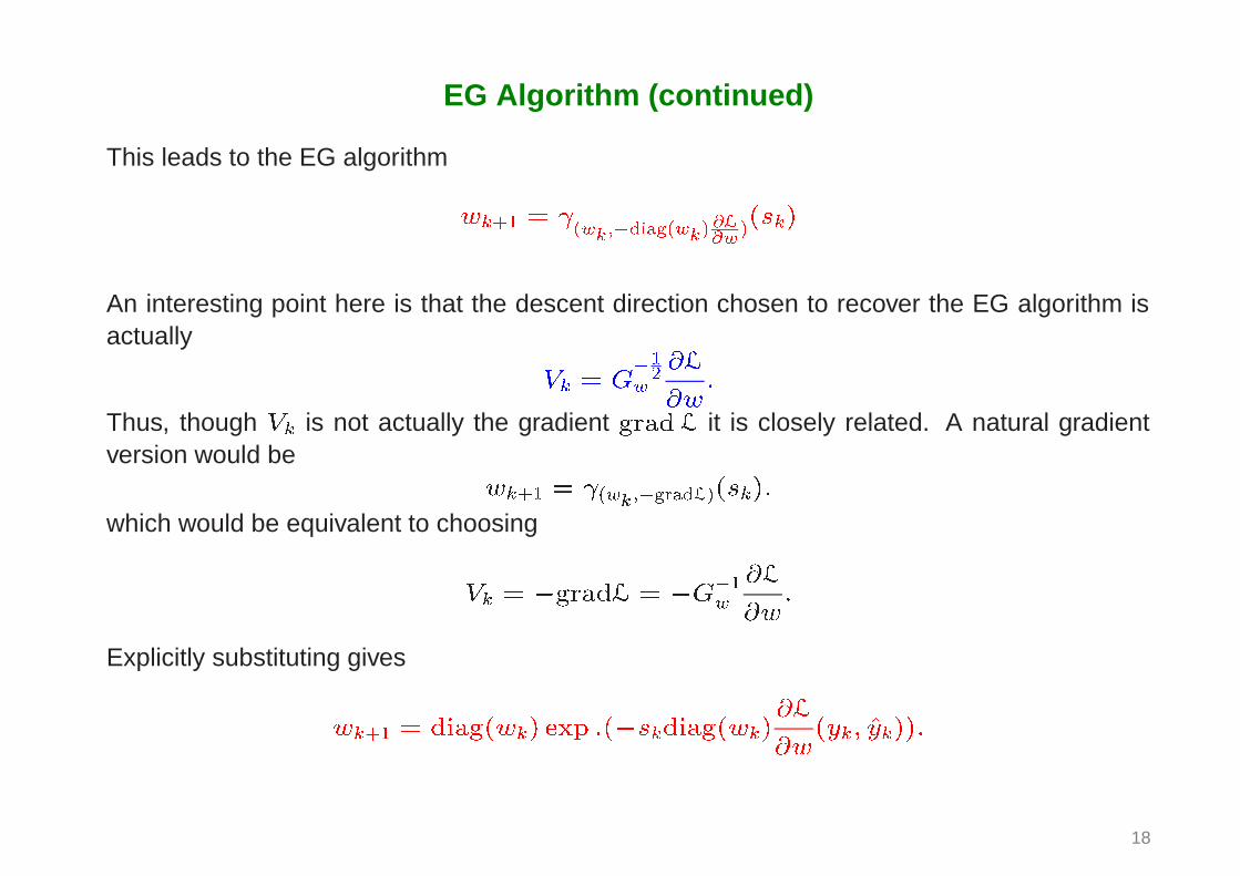
EG Algorithm (continued)

This leads to the EG algorithm

��

��

An interesting point here is that the descent direction chosen to recover the EG algorithm isactually

��

�

��

Thus, though �� is not actually the gradient �� it is closely related. A natural gradientversion would be

��

which would be equivalent to choosing

��

�

��

Explicitly substituting gives

��

��

18

THE LINK WITH LINK FUNCTIONS

Consider a product preferential metric of the form

��

��

� . . . ...... . . . ...

� � ��

� �

where �� are positive definite functions �� . Note that each ��

is chosen to depend only on its associated variable. This is the case when the �� areindependent prior distributions associated with a product prior ��

��

Theorem Suppose �� for all � � � . Then the solution of the geodesic equation is

��!� � ��

� �!�� (21)

where ��

�� (the indefinite integral of �).

19

Algorithm in terms of �

By setting � � ��, and since

��

�

��

� ��

� ��

� ��

�

(17) takes the general form

��

� ��

��

��

��

�

��

��

When � is the squared loss (3), �� and

��

��

�

��

��

��

� ��

��

(22)

20

Possible choices of �, � and �� for algorithm (22).

Algorithm �� Conditions ��

EGnatural�

�

� � � ��

EG(�)

��

� � �

� ��

�

��

��

�

��

�

��

EGclipped() ��

��

� � �

��

��

��

��

��

� ��

Cauchy��

��

��

Cauchy

�

� � ��

��

Cauchy��

�

��

��

��

��

��

��

�

��

��

�

��

Gaussian ��

��

��

��

�

�

21

SIMULATIONS

In order to present simulation results, it was necessary to decide on an appropriate way tocompare the different algorithms, and in particular how to choose the step size parameter ��.The options available to choose �� include:

Following Amari one may argue that the asymptotic stability of the algorithm is an adaquatemeasure of performance. Thus, any sufficiently small step-size selection is satisfactory.

Pick the “optimal” �� according to Kivinen and Warmuth. The way they do this dependson knowledge of the sequence of examples and the true weight vector.

Adopt the standard signal processing method of comparison: determine steady-state MeanSquare Error (MSE) as a function of �, and then choose � to achieve a fixed steady-stateMSE. Then compare algorithms in terms of their speed of convergence.

Adopt the choice implied by the analysis in terms of � (see full paper). This is what we didfor the simulations below.

22

Details of Simulations�� was drawn independently from a uniform distribution on ��

�� , � � ��. The step-

size for the GD algorithm was � � � ��. Step sizes for the other algorithms were chosen“fairly” chosen according to new theorem (not presented here).

The target had the non-zero values inferrable from the diagram, with all the remaining valueszero (a fraction of �� of the dimensions of �� were non-zero).

Gaussian noise of standard deviation �� was added to the �� sequence.

Both algorithms were started from the initial condition � ��

��. In the graphs, only

the first �� dimensions of �� have been plotted for the sake of clarity.

The indicated Mean Square Errors (MSE) were estimated from the final fifth of the run.

23

0 500 1000 1500 2000 2500 3000−2

−1

0

1

2GD, mse= 2.4

0 500 1000 1500 2000 2500 3000−2

−1

0

1

2Exp( 0.9), mse= 1.2

Figure 1: Comparison of � ��"� (" � ��) algorithm with standard Gradient Descent.

24

0 500 1000 1500 2000 2500 3000−2

−1

0

1

2GD, mse= 2.4

0 500 1000 1500 2000 2500 3000−2

−1

0

1

2Exp( 0.1), mse= 2.1

Figure 2: Same as Figure 1 except with " � ��

25

0 500 1000 1500 2000 2500 3000−2

−1

0

1

2GD, mse= 2.4

0 500 1000 1500 2000 2500 3000−2

−1

0

1

2Exp( 1.1), mse= 1.1

Figure 3: Same as Figure 1 except with " � ��

26

Details of Remaining simulations

Step size for EGclipped�#� chosen according to new theorem (not described here).

The target had the non-zero values inferrable from the diagram, with all the remaining valueszero (a fraction of �� of the dimensions of �� were non-zero).

Gaussian noise of standard deviation �� was added to the �� sequence. Both algorithmswere started from the initial condition � �

��

��.

In the graphs, only the first �� dimensions of �� have been plotted for the sake of clarity. Theindicated Mean Square Errors (MSE) were estimated from the final fifth of the run.

27

0 500 1000 1500 2000 2500 3000−2

−1

0

1

2GD, mse=0.019

0 500 1000 1500 2000 2500 3000−2

−1

0

1

2EGclipped( 3), mse=0.0062

Figure 4: Comparison of the EGclipped�#� algorithm (# � �), �� drawn iid uniformlyon ��

��

�� , (� � ��), � � � ��.

28

0 500 1000 1500 2000 2500 3000−2

−1

0

1

2GD, mse=0.019

0 500 1000 1500 2000 2500 3000−2

−1

0

1


Figure 5: Same as Figure 1 except with # � ��.

29

0 500 1000 1500 2000 2500 3000−2

−1

0

1

2GD, mse=0.019

0 500 1000 1500 2000 2500 3000−2

−1

0

1


Figure 6: Same as Figure 1 except with # � �.

30

CONCLUSIONS Have shown how to modify traditional stochastic gradient descent algorithms to take

account of prior information encoded as a Bayesian prior ��.

The Exponentiated Gradient (EG) algorithm can be interpreted in terms of a prior of theform ��

�� $��.

Suggested the use of the natural gradient.

The use of natural gradient and related geometric machinery is different to the work doneby Amari (he assumes he knows the likelihood function, and exploits that, but presumes auniform or an uniformative prior). In principle could combine both approaches.

In the full paper (not done here) we have also shown that the algorithm designed from � isthe “best” in a probabilistic sense. (This is rather intricate to set up, in order to make thecomparison fair — not the least of the difficulties are in chosing the step size.)

Approach shows how to create a wide range of variations on GD.

Have already had success in applying the ideas to a communications problem.

31

Further Details

Further details can be found in the full version of this paper:

Robert E. Mahony and Robert C. Williamson, “Prior Knowledge and PreferentialStructures in Learning Algorithms,” submitted to Journal of Machine Learning Research,August 2000. http://theorem.anu.edu.au/˜williams/papers/P102.ps.gz

32

riemannian structure of some new gradient descent learning algorithms

Documents