riemannian geometry - ut mathematics · m392c notes: riemannian geometry arun debray may 4, 2017...

RiemannianGeometry

UT Austin, Spring 2017

M392C NOTES: RIEMANNIAN GEOMETRY

ARUN DEBRAYMAY 4, 2017

These notes were taken in UT Austin’s M392C (Riemannian Geometry) class in Spring 2017, taught by Dan Freed. Ilive-TEXed them using vim, so there may be typos; please send questions, comments, complaints, and corrections [email protected]. Any mistakes in the notes are my own. Thanks to Martin Bobb, Gill Grindstaff, JonathanJohnson, and Sebastian Schulz for some corrections.

The cover image is the Cosmic Horseshoe (LRG 3-757), a gravitationally lensed system of two galaxies. Einstein’stheory of general relativity, written in the language of Riemannian geometry, predicts that matter bends light, so if twogalaxies are in the same line of sight from the Earth, the foreground galaxy’s gravity should bend the backgroundgalaxy’s light into a ring, as in the picture. The discovery of this and other gravitational lenses corroborates Einstein’stheories. Source: https://apod.nasa.gov/apod/ap111221.html.

Contents

1. Geometry in flat space: 1/17/17 32. Existence of Riemannian metrics: 1/19/17 73. The curvature of a curve: 1/24/17 104. Curvature for surfaces: 1/26/17 145. Extrinsic and intrinsic curvature: 1/31/17 176. Vector fields and integral curves: 2/2/17 217. Tangential structures of manifolds: 2/7/17 248. Distributions and Foliations: 2/9/17 279. Lie algebras and Lie groups: 2/14/17 3110. The Maurer-Cartan form: 2/16/17 3511. Characterizing the Maurer-Cartan form: 2/21/17 3812. Applications to immersed surfaces: 2/23/17 4113. Principal G-bundles: 2/28/17 4314. Connections on frame bundles: 3/2/17 4715. The Levi-Civita connection and curvature: 3/7/17 4916. Covariant derivatives: 3/9/17 5217. Symmetries of the Riemann curvature tensor: 3/21/17 5618. Constant curvature and holonomy: 3/23/17 5919. Holonomy and Kähler manifolds: 3/28/17 6220. Complex manifolds: 3/30/17 6521. : 4/4/17 6922. Irreducibility : 4/6/17 6923. Homogeneous spaces, I: 4/11/17 6924. Homogeneous spaces, II: 4/13/17 7225. Affine local diffeomorphisms: 4/18/17 7426. Locally symmetric spaces: 4/20/17 7727. Geodesics: 4/25/17 8028. Spectral geometry: 5/2/17 8229. : 5/4/17 86

2

mailto:[email protected]?subject=M392C%20Lecture%20Notes

https://apod.nasa.gov/apod/ap111221.html

1 Geometry in flat space: 1/17/17 3

Lecture 1.

Geometry in flat space: 1/17/17

“Do you have all these equations?”Before we begin with Riemannian manifolds, it’ll be useful to do a little geometry in flat space.

Definition 1.1. Let V be a real vector space; then, an affine space over V is a set A with a simply transitiveright V-action.

That this action is simply transitive means for any a, b ∈ A, there’s a unique ξ ∈ V such that a · ξ = b.

Definition 1.2. A set with a simply transitive (right) V-action is called a (right) V-torsor.

V-torsors look like copies of V without a distinguished identity.One of the distinct features of affine space is global parallelism: if I have a vector ξ at a point a, I

immediately get a vector at every point, which defines a vector field on the entire space.What is the analogue of a basis for an affine space? This is a collection of points a0, . . . , an such that any

a ∈ A is uniquely written as

(1.3) a = λ0a0 + λ1a1 + · · ·+ λnan

for some λi ∈ R with λ0 + · · ·+ λn = 1.Equation (1.3) may be written more concisely with index notation: any variable written as both a

superscript and a subscript is implicitly summed over. That is, we may rewrite (1.3) as

a = λiai.

Note that in an affine space, we don’t know how to add vectors (since we don’t have an origin), but we cantake weighted averages.

Theorem 1.4 (Giovanni Ceva, 1678). Let A be an affine plane and a, b, c ∈ A be a triangle (i.e. three distinct,noncollinear points). Suppose p ∈ bc, q ∈ ca, and r ∈ ca. Then, ap, bq, and cr are coincident iff

[ar : rb][bp : pc][cq : ca] = 1.

Typically, this is thought of as a ratio of lengths, but we don’t necessarily have lengths: instead, we canuse barycentric coordinates. There is a unique λ such that if r = (1− λ)a + λb, then [ar : rb] = λ/(1− λ).

Proof. Let

r := (1− λ)a + λb

p := (1− µ)b + µc

q := (1− ν)c + νa.

Set

(1.5) x := αa + βb + γc,

where α + β + γ = 1. Since x ∈ ap, then

(1.6) x = αa + C((1− µ)b + µc).

Comparing (1.5) and (1.6), µ/(1− µ) = γ/β.

Standard affine space An := (x1, . . . , xn) ∈ Rn | xi ∈ R. You may complain this is the same as Rn, butAn only comes with an affine structure, not a vector-space structure.

Definition 1.7. Let A be an affine space modeled on V and B be an affine space modeled on W. Then, amap f : A→ B is affine if there exists a linear map T : V →W such that f (a + ξ) = f (a) + Tξ for all a ∈ Aand ξ ∈ V.

In other words, an affine map is a linear map plus some constant, which is not uniquely defined.

Definition 1.8. An affine coordinate system on A is an affine isomorphism x = (x1, . . . , xn) : A→ An.

4 M392C (Riemannian Geometry) Lecture Notes

a

b

cq

r p

Figure 1. Depiction of Ceva’s theorem (Theorem 1.4).

Them, the differentials dx1a , . . . , dxN

a are independent of basepoint a and form a basis for V∗, the dualvector space and dual basis to V and ∂

∂x1 , . . . , ∂∂xn , the tangent space to any a ∈ A.

But affine space is not the only flat geometry we could consider: more generally, we consider a structureon a vector space V which can be promoted to a translationally invariant structure on A. This leads tometric geometry, symplectic geometry, etc.

Definition 1.9. An inner product on a (finite-dimensional) vector space V is a bilinear map 〈–, –〉 : V×V → Rwhich is symmetric and positive definite, i.e. for all ξ, η ∈ V, 〈ξ, η〉 = 〈η, ξ〉, 〈ξ, ξ〉 ≥ 0, and 〈ξ, ξ〉 = 0 iffξ = 0.

Since 〈–, –〉 is bilinear, then this can be determined in terms of n2 numbers: let v1, . . . , vn be a basis for Vand define gij := 〈vi, vj〉 for i, j = 1, . . . , n. Of course, these numbers areen’t independent: gij = gji, so thereare really only n(n + 1) choices of information.

Definition 1.10. A basis e1, . . . , en for V is orthonormal if

〈ei, ej〉 = δij :=

1, i = j0, i 6= j.

.

Our first major result of flat Euclidean geometry is that these exist.

Theorem 1.11. There exist orthonormal bases.

Proof. Let v1, . . . , vn be any basis of V. Let

e1 =v1

〈v1, v1〉1/2 ,

and for i = 2, . . . , n, letv′i = vi − 〈vi, e1〉e1.

Then, 〈e1, e1〉 = 1 and 〈e1, v′i〉 = 0. Then, repeat with v′2, . . . , v′n.

This explicit algorithm is called the Gram-Schmidt process.In an inner product space, we get some familiar geometric constructions: the length of a vector ξ ∈ V is

|ξ| = 〈ξ, ξ〉1/2, and the angle between ξ, η ∈ V \ 0 is the θ such that

cos θ =〈ξ, η〉|ξ||η| .

Definition 1.12. A Euclidean space E is an affine space over an inner product space V.

This has a notion of distance: dE : E× E→ R≥0, where a, b 7→ |ξ|, where b = a + ξ. This generalizes tonotions of area, volume, etc.

Theorem 1.13 (Napoleon, 1820). Let abc be a triangle in a plane and attach an equilateral triangle to each edge.The centers of these three triangles form an equilateral triangle.

Exercise 1.14. Prove this.

B ·C


We want to understand curved analogues of this classical material, and will pick up where differentialtopology left off. We work on smooth manifolds: a smooth manifold is a space X together with an atlas ofcharts U ⊂ X with homeomorphisms x : U → An such that every point is contained in the domain of somechart and the transition maps are smooth. We do not require a manifold to have a global dimension: thedifferent connected components may have different dimensions, e.g. S1 q S2.1

A chart map x : U → An is a set of n continuous maps (x1, . . . , xn). If p is in the domain of both x and y,we can consider x y−1 : An → An; calculus as usual tells us what it means for this transition map to besmooth.

At any x ∈ X, we have a tangent space TxX and a cotangent space TxX: a chart defines a basis of thetangent space ∂

∂x1 , . . . , ∂∂xn and a basis of the contangent space dx1

x, . . . , dxnx . This depends strongly on x:

unlike for flat space, we may not be able to parallel-transport these globally, even on something as simpleas S2.

In this course, we will study what happens when we go from a curved analogue of affine space to acurved analogue of Euclidean space, whence the following central definition.

Definition 1.15. A Riemannian metric on a smooth manifold X is a choice of inner product 〈–, –〉x on TxXfor all x ∈ X which varies smoothly in x.

Now, we can compute lengths of tangent vectors and the angle that two smooth curves intersect at (orrather, the angle their tangent vectors intersct at). We also obtain a notion of distance between points, andcan develop analogues of Euclidean geometry on manifolds.

What does “varying smoothly” mean, exactly? Suppose x1, . . . , xn is a set of local coordinates on U ⊂ X;then, for i, j = 1, . . . , n, define

gij :=⟨

∂

∂xi

∣∣∣∣x

,∂

∂xj

∣∣∣∣x

⟩TxX

.

One can check that if the metric is smoothly varying in one chart, then it’s smoothly varying in all charts.We’ll write the metric as

g = gij dxi ⊗ dxj.

This again uses the summation convention, and it’s useful to think about where exactly this lives: itidentifies the metric as a tensor.

Many manifolds arise as embedded submanifolds of Euclidean space, and the Whitney embeddingtheorem shows that all may be emnbedded. Many authors say it’s best to meet manifolds as embeddedsubmanifolds first, but there are some which arise without a natural embedding, e.g. the GrassmanianGr2(R4), the space of two-dimensional subspaces of R4.

In any case, if X ⊂ EN is embedded, then X inherits a metric, since TxX ⊂ Rn is also a subspace, and wecan restrict the inner product. Classical Riemannian geometry is the study of plane curves (one-dimensionalsubmanifolds of R2), space curves (one-dimensional submanifolds of R3), and surfaces (two-dimensionalsubmanifolds of R3).

To study Riemannian manifolds, we should begin with the simplest cases. The zero-dimensionalmanifolds are disjoint unions of points with zero-dimensional tangent spaces and the trivial Riemannianmetric. In the one-dimensional case, there is a little more to tell. A smooth map X → Y of Riemannianmanifolds is an isometry if it’s a map that preserves the inner product on each tangent space. Thisautomatically implies it’s injective.

Theorem 1.16. Let C be a (complete) Riemannian 1-manifold which is diffeomorphic to R. Then, C is isometric toE1.

Before we prove this, we need a change-of-coordinates lemma. (We’ll address completeness later, toavoid finite intervals.)

Remark 1.17. Let x1, . . . , xn and y1, . . . , yn be coordinate systems and suppose a metric can be written as

g = gij dxi ⊗ dxj = hab dya ⊗ dyb.

1This is important for, e.g. a space of solutions of certain PDEs.


Then,

(1.18) gij = hab∂ya

∂xi∂yb

∂xj .

This is n2 equations: there is no implicit summation here. (

Proof of Theorem 1.16. Let x : C → R be a diffeomorphism, which defines a global coordinate on C. Letg(x) = 〈 ∂

∂x , ∂∂x 〉. We seek a new coordinate y : C → R such that h(y) = 〈 ∂

∂y , ∂∂y 〉 = 1 everywhere. By (1.18),

(1.19) g =

(dydx

)2,

so fix an x0 ∈ C and define

y(x) =∫ x

x0

√g(t)dt.

This y satisfies (1.19) and therefore is an isometry.

The analogue to Theorem 1.16 in n dimensions (where n > 1) is as follows: if x1, . . . , xn is a localcoordinate system and gij is the Riemannian metric in these coordinates, is there a local change ofcoordinates ya(x1, . . . , xn) such that hab = δab? This is the analogue in Riemannian geometry to findingorthonormal coordinates, guaranteed by Theorem 1.11.

This requires solving an analogue to (1.18), but this time it’s a PDE

gij = ∑a

∂ya

∂xi∂ya

∂xj .

This time, we need to ask whether there are solutions. The only thing we know how to do is differentiate:

(1.20a)∂gij

∂xk = ∑a

∂2ya

∂xk∂xi∂ga

∂xj +∂ya

∂xi∂2ya

∂xk∂xj .

By permuting indices, we obtain

∂gik

∂xj = ∑a

∂2ya

∂xj∂xi∂ga

∂xk +∂ya

∂xi∂2ya

∂xj∂xk(1.20b)

∂gjk

∂xi = ∑a

∂2ya

∂xi∂xj∂ga

∂xk +∂ya

∂xj∂2ya

∂xi∂xk .(1.20c)

Taking (1.20a) + (1.20b)− (1.20c), we obtain

12

(∂gij

∂xk +∂gik

∂xj −∂gjk

∂xi

)= ∑

a

∂ya

∂xi∂2ya

∂xj∂xk .

Now we multiply by ∂yb

∂x` gì, concluding

∂yb

∂x`gì

2

(∂gij

∂xk +∂gik

∂xj −∂gjk

∂xi

)Γ`

jk

= ∑a

∂ya

∂xi∂2ya

∂xj∂xk gì ∂yb

∂x`.

These Γ`jk symbols therefore satisfy

∂2yb

∂xj∂yk = Γijk

∂yb

∂xi .

If we differentiate once again (with respect to x`), we get

∂3yb

∂x`∂xj∂xk =∂Γi

jk

∂x`∂yb

∂xi + Γijk

∂2yb

∂x`xi

=

(∂Γi

jk

∂x`+ Γm

jkΓim`

)∂yb

∂xi .


Since mixed partials commute, then one discovers that if such an isometry exists, the Riemannian curvaturetensor

(1.21) Rijk` :=

∂Γij`

∂x`−

∂Γijk

∂x`+ Γm

jkΓim` − Γm

j`Γimk

must vanish. In simple cases, one can calculate that it’s not always zero, so we don’t always have globalparallelism.

Riemann derived this in the middle of the 1800s. It’s possible to see the glimmer of special relativity inthem, though of course this was discovered later.

There’s no text, though there is a website: http://www.ma.utexas.edu/users/dafr/M392C/index.html.There are problem sets, so undergraduates have to do some problem sets, and graduate students should.Feel free to talk to the professor about the problems, and especially to establish groups to work on theproblem sets. Office hours are Wednesdays 2 to 3.

Lecture 2.

Existence of Riemannian metrics: 1/19/17

“There are so many of you. . . so quiet. . . I’ll be more provocative until I get questions. Or I’ll gofaster.”

Due to the large size of the class, it’s being moved to RLM 6.104 starting next week. This means everyonewho wants to sign up should be able to.

Some readings are up on the website, including a translation of Riemann’s original work on curvature.Last time, we defined affine space, which leads to the notion of a smooth manifold, and then introduced

Euclidean space, an affine space over an inner product space. The curved version of that is a Riemannianmanifold.

Recall that a Riemannian metric g on a smooth manifold X is a smoothly varying family of innerproducts on TxX, and a Riemannian manifold is a smooth manifold together with a Riemannian metric.We also defined an isometry: if X and Y are Riemannian manifolds, then a diffeomorphism f : X → Y isan isometry if for all x ∈ X and ξ1, ξ2 ∈ TxX,

〈 f∗ξ1, f∗ξ2〉Tf (x)Y= 〈ξ1, ξ2〉TxX .

Here, f∗ : TxX → Tf (x)Y is the linear pushforward of tangent vectors, also called the differential. If f ismerely a smooth function, this is called an isometric immersion (the inverse function theorem automaticallyimplies it’s an immersion). If f is an embedding, this is called an isometric embedding.

Existence of Riemannian metrics. Suppose V is a real vector space and g0, g1 : V × V → R are innerproducts. Then for t ∈ [0, 1], (1− t)g0 + tg1 is also an inner product (you can check this directly).

The set of bilinear maps V ×V → R, denoted Bil(V ×V,R), is a real vector space, naturally isomorphicto Hom(V ⊗ V,R) and to V∗ ⊗ V∗. Here, “natural” means this works for all finite-dimensional vectorspaces at once, and commutes with linear maps.

Inner products are elements of this vector space, and our observation above means that if g0 and g1are inner products, the line between them in Bil(V ×V,R) consists of inner products. In particular, innerproducts form a convex set. This only uses the affine structure on Bil(V ×V,R), since we can take convexcombinations in an affine space.

This is used to generalize to the curved case, showing Riemannian metrics always exist.

Theorem 2.1. Let X be a smooth manifold. Then, there is a Riemannian metric on X.

Proof. Let U = (U, x) be a cover of X by coordinate charts x : U → An, and let gU denote the metric onU such that ∂

∂x1 , . . . , ∂∂xn are orthonormal. That is, take the standard metric on An making it into Euclidean

space En, and pull it back to U, where it becomes a metric (you can check that metrics pull back alongclosed immersions).

Now, the bases on two different charts in U don’t agree, and don’t necessarily differ by orthonormalbases. Thus, we use a standard argument in differential geometry to globalize local objects living in a

http://www.ma.utexas.edu/users/dafr/M392C/index.html


convex set: let ρUU∈U be a partition of unity subordinate to U; then,

g = ∑U∈U

ρU gU

is a Riemannian metric.

Remark 2.2. Global existence is not assured for every geometric structure. For example, a complex structureon a real vector space V is an endomorphism J : V → V such that J2 = −idV . This is akin to multiplicationby i in a complex vector space, which squares to −1 and commutes with addition.

You can place this structure on affine space, and there’s an immediate obstruction: dimR V must be even.Now we globalize: given an even-dimensional manifold, do we have such a structure? That is, can we placea smoothly varying complex structure on TxX for all x ∈ X? This is called an almost complex structure, andnot every even-dimensional manifold admits one.

Exercise 2.3. Show that S4 has no almost complex structure.

There is an almost complex structure on S6, and it’s a famous open question whether there’s a complexstructure (i.e. complex coordinates with holomorphic transition functions). The known almost complexstructure does not work.

Another local structure that doesn’t automatically globalize is a mixed-signature metric (e.g. a Minkowskimetric). In such a metric, the null vectors, those ξ for which 〈ξ, ξ〉 = 0, form a cone whose interior is thepositive vectors (for which the metric is positive). Trying to globalize this produces, more or less, a line ineach tangent space TxX. Passing to a double cover, one can choose an orientation, and therefore a nonzerovector field on X, and this can’t be done in general. For example, a surface of genus 2 admits no metric ofsignature (1, 1). These kinds of metrics arise in general relativity. (

In this class, we care about Riemannian metrics, which do globalize.Let x1, . . . , xn be local coordinates; then, we defined some local quantities in the metric in terms of these

coordinates. Namely,

gij =

⟨∂

∂xi ,∂

∂xj

⟩,

so that g = gij dxi ⊗ dxj = gij dxi dxj. We then used this to define symbols Γijk and the Riemann curvature

tensor Rijk`. We proved Theorem 1.16; here’s a better version.

Theorem 2.4. Let C be a Riemannian 1-manifold diffeomorphic to R. Then, there exists an isometry C → I, whereI ⊂ E1 is an open interval.

The argument we gave defining the Riemann curvature tensor generalizes this.

Theorem 2.5. Suppose (U, g) is a Riemannian manifold and x : U → An is a global coordinate such that

g =n

∑i=1

(dxi)2.

Then, Rijk` = 0 on U.

One important thing to check here is that

R = Rijk`

∂

∂xi ⊗ dxj ⊗ dxk ⊗ dx`

is independent of the coordinate system (which is not clear from its definition). This means that theRiemann curvature tensor is a tensor, i.e. R ∈ TxX ⊗ T∗x X ⊗ T∗x X ⊗ T∗x X. In the next few weeks, we willadd some geometry to this discussion.

Example 2.6. Let X = E2 be Euclidean space with the standard metric g. Then, we have global coordinates(x, y) : E2 → A2, so g = dx2 + dy2.

We can also introduce polar coordinates, another coordinate system which isn’t global. This is a coordinatemap (r, θ) : E2 \ (x, 0) : x ≤ 0 → A2 (so r > 0, −π < θ < π). In this case, the metric has the form

g = dr2 + r2 dθ2.

This means that the vector field ∂∂r has constant length 1, but the vector field ∂

∂θ has length r at (r, θ). (

2 Existence of Riemannian metrics: 1/19/17 9

Symmetry. We’ve now seen vector spaces, affine spaces, Euclidean spaces, and Riemannian manifolds. Asin any mathematical context, it’s important to ask what the proper notion of symmetry is for these objects.

If V is a vector space, its general linear group is GL(V) = Aut(V) := T : V → V invertible. The standardexample is GLn(R) := GL(Rn), the group of invertible n× n matrices, acting on the column vectors of Rn

by scalar multiplication. For example GL1(R) = R×, the group of nonzero numbers under multiplication.What about affine space? Affine space on V is a V-torsor, as V acts by translation. The symmetry group

is the group of affine transformations

Aff(A) := α : A→ A | α is invertible and affine.

Recall that an affine map is one that preserves the affine structure: the image of a finite weighed average isthe weighted average of the images. The derivative of an affine map is a linear map, so if A is an affinespace modeled by V, the derivative defines a group homomorphism d : Aff(A)→ GL(V), whose kernel isthe translations, a group isomorphic to V. Thus, we have a group extension (short exact sequence of groups)

(2.7) 1 // V // Aff(A)d // GL(V) // 1.

The key is that in affine space, there’s no canonical origin. However, (2.7) splits, if noncanonically: choosean a ∈ A. Then, any b ∈ A can be uniquely written as a+ ξ for some ξ ∈ V, so for any linear transformationT, a + ξ 7→ a + Tξ is an affine transformation of A.

(2.7) is a sequence of manifolds with smooth group homomorphisms, making it a short exact sequenceof Lie groups; we’ll discuss Lie groups more later.

If V is an n-dimensional vector space, its bases are the set B(V) = b : Rn ∼=→ V. If V = Rn, this isGLn(R). In general, this makes B(V) into a right GLn(R)-torsor, defined by the simply transitive actionB(V)×GLn(R)→ B(V) sending β, g 7→ β g. (There is a corresponding left action by GL(V)). The actionon the right is akin to numbering elements of the basis, and the action on the left is more geometric; this isan instance of a general idea that internal actions tend to be from the right, and geometric ones from theleft.

What’s the analogue for an affine space A modeled on V? Let B(A) denote the collection of pairs (a, β)

where a ∈ A and β ∈ B(V), identified with the set of affine isomorphisms α : A∼=→ An. These are the

bases at specific points of A. There is a forgetful map π : B(A) → A sending (a, β) → a, and the fiberis B(V), the bases at a. In a similar way, there is a left action of Aff(A) on B(A), and a right action ofAffn := Aff(An) on B(A).

We’ll use these torsors of bases a lot in this class. In this way, we’re enacting Felix Klein’s Erlangenprogram, where the kind of geometry we do is reflected by the symmetry group we place on the geometricstructures.

Let’s see what happens to these ideas in the Euclidean and Riemannian cases. If V is an inner productspace, its orthogonal group O(V) ⊂ GL(V) is the group of linear isomorphisms preserving the inner product,i.e. T : V → V such that 〈Tξ1, Tξ2〉 = 〈ξ1, ξ2〉 for all ξ1, ξ2 ∈ V. For V = Rn, we let On := O(Rn).

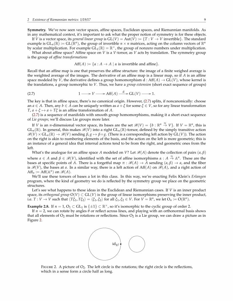
Example 2.8. If n = 1, O1 ⊂ GL1 is ±1 ⊂ R×, so it’s isomorphic to the cyclic group of order 2.If n = 2, we can rotate by angles θ or reflect across lines, and playing with an orthonormal basis shows

that all elements of O2 must be rotations or reflections. Since O2 is a Lie group, we can draw a picture as inFigure 2.

idR2

Figure 2. A picture of O2. The left circle is the rotations; the right circle is the reflections,which in a sense form a circle half as long.


As with the affine symmetries, there’s an extension

1 // SO2 // O2 // ±1 // 1. (

Similarly, the isomorphisms of Euclidean space E, denoted Euc(E), are the affine isomorphisms preserv-ing the inner product at each point. This again fits into an extension sequence

1 // V // Euc(E) // O(V) // 1.

All this is nice, but let’s talk about manifolds. If X is a smooth manifold, we no longer have translations,and the linear symmetries talk about the tangent space. We’ll see what kind of structures we get in thiscase.

The analogue of the torsor of bases is B(X) := (x, β) : x ∈ X, β : Rn ∼→ TxX. This admits a right actionof GLn(R) by precomposition, as on a vector space, and there is again a forgetful map π : B(X)→ X thatignores the basis.

If x : U → An is a chart, then it defines a local section U → B(X) sending

(x1, . . . , xn) 7−→((x1, . . . , xn),

(∂

∂x1 , . . . ,∂

∂xn

)).

If X is a Riemannian manifold, then we can also speak of orthonormal bases:

BO(X) := (x, β) : x ∈ X, β : Rn ∼=→ TxX is an isometry.Again there is a forgetful map to X, but now a coordinate does not always determine a section: if theRiemann curvature tensor doesn’t vanish, the image of an orthonormal basis of the tangent space at a pointmight not be orthonormal.

B(X) and BO(X) are not just sets but smooth manifolds, and the forgetful maps back to X are calledfiber bundles (even principal bundles). We’ll go back and discuss this in more detail.

Curvature. Let’s end with something concrete. Let E be a Euclidean plane, an affine space with anunderlying 2-dimensional inner product space.

Let C ⊂ E be a 1-dimensional submanifold. Let’s choose a co-orientation of C: an orientation of C is anorientation of its tangent bundle, so a co-orientation is an orientation of its normal bundle. In essence, thisis choosing a side of the curve.2 We’ll use this to define a function κ : C → R called the (signed) curvature.Intuitively, this should be positive if C is curved towards the side chosen by the co-orientation, and negativeif it curves away, and a larger magnitude means a stronger curvature.

The Euclidean structure on E induces an inner product structure on TxC for all x ∈ C that variessmoothly, so C becomes a Riemannian manifold. Theorem 1.16 means there’s nothing intrinsic about C wecan measure, but the way in which it sits inside E is what κ will measure. This is an important dichotomy,between intrinsic geometry and extrinsic geometry. The Riemann curvature tensor is intrinsic, since itdoesn’t depend on an embedding, but the signed curvature will be extrinsic.

Lecture 3.

The curvature of a curve: 1/24/17

“And if you follow your nose. . . well, Euler’s nose. . . ”In the next two lectures, we’ll march through the theory of extrinsic curvature (which can fill an entireundergraduate course).

Let E be a Euclidean plane modeled on an inner product space of V, which acts on E by translations, andlet i : C → E be an immersed 1-manifold.3 Suppose C is co-oriented, meaning we’ve oriented its normalbundle (picking a side of C, so to speak). This determins a unit co-oriented normal vector e1 at every x ∈ C,meaning the unique unit vector in (νC→E)x with a positive orientation. We can also choose a unit tangentvector e2 perpendicular to e1, and there are two choices. Together they define an orthonormal basis at eachpoint: (e1, e2) : C → BO(V).

2If N → M is an embedding and M is oriented, an orientation of N and a co-orientation of N determine each other.3Especially if C is immersed but not embedded, it is helpful to remember i: when C self-intersects, remembering i is necessary for

computing curvature.

3 The curvature of a curve: 1/24/17 11

You learned how to do calculus with real-valued differential forms; in exactly the same way, it’s possibleto do calculus with vector-valued differential forms Ω∗C(V), the forms modeled on functions C → V. Fori, j ∈ 1, 2, we can define ei ∈ Ω0

C(V) and dei ∈ Ω1C(V), such that 〈ei, ej〉 = δij and the Leibniz rule is

satisfied:〈dei, ej〉+ 〈ei, dej〉 = 0.

Thus, there exists an α ∈ Ω1C such that

de1 = −αe2 and de2 = αe1.

In other words, applying d to the row vector (e1 e2) multiplies it by a skew-symmetric matrix:

d(e1 e2

)=(e1 e2

) ( 0 α−α 0

).

Let θ1, θ2 : C → V∗ define the dual basis at each point, i.e. at every x ∈ C, θi(ej) = δij as functions C → R.

Then, i∗θ2 ∈ Ω1C and we can write

α = k · i∗θ2

for some function k : C → R.

Definition 3.1. The curvature of C is the function k.

Example 3.2. Let C denote the circle of radius R in the Euclidean plane E2. It’s parameterized by coordinatesx = R cos φ and y = R sin φ, so

dx = −R sin φ dφ

dy = R cos φ dφ.

Let’s choose the co-orientation in which the inward-pointing unit normal is positively oriented. Then,

e1 = − cos φ∂

∂x− sin φ

∂

∂y.

We also have to choose e2: suppose it points clockwise along the circle. Then,

e2 = sin φ∂

∂x− cos φ

∂

∂y.

Thus, the dual basis is defined by

θ1 = − cos φ dx− sin φ dy

θ2 = sin φ dx− cos φ dy,

so i∗θ2 = R dφ. Then,

de2 = cos θ dθ∂

∂x+ sin θ dθ

∂

∂y= −dθe1.

Thus, de2 = (1/R)i∗θ2(e1). In particular, the curvature is 1/R. It has units of 1/length.If we chose e2 to point counterclockwise, there would be a sign change in θ2, and another one in α, so

they would cancel out to give the same result. (

Since the unit vector always has unit length in V, you can think of e1 as a map C → S(V) (called theGauss map), where S(V) is the unit sphere inside V. At a point p ∈ C, we can define the tangent line TpC ati(p); the tangent line is a subspace of V. We can also consider the tangent line to e1(p) ∈ S(V), Te1(p)S(V);both of these are the same space, the space of vectors in V perpendicular to e1(p).

This means the differential

(3.3) (de1)p : TpC −→ Te1(p)S(V)

is a map from a line to itself.

Theorem 3.4. The map in (3.3) is multiplication by −k(p).

Proof.de1(e2) = α(e2) · d2 = −ki∗θ2(e2)e2 = −k · e2.


Remark 3.5 (History). The curvature may have been initially defined by Nicole Oresme in about 1350. Itwas again discovered by Huygens in c. 1650 and Newton in c. 1664. (

Here’s a third approach to curvature. Let i : C → E be a co-oriented curve as usual, and assume C isembedded. For some p ∈ C, we can identify the normal line to i(p) with R, letting the positive numberspoint into the positively oriented direction. Call this coordinate y. Given a choice of a unit tangent vectore2, we can identify the tangent line with R, again pointing the positive numbers in the x-direction. Call thiscoordinate x.

Lemma 3.6. There exists an open set U ⊂ E about p such that C ∩U is the graph of a function f : R→ R in theabove xy-coordinate system such that

• f (0) = f ′(0) = 0, and• f ′′(0) = k(p).

Proof. The x-coordinate map x|C : C → R satisfies dxp = idTpC; in particular, it’s invertible. By the inversefunction theorem, there’s a local inverse g : I → C, where I ⊂ R is an open interval. Define f to be y i g:since i : C → E and y : E→ R, this is a map I → R. Write

e1 =(− f ′, 1)√1 + ( f ′)2

and e2 =(1, f ′)√1 + ( f ′)2

.

Then,

de1 =

((− f ′′, 0)√1 + ( f ′)2

+(− f ′, 1)

(1 + ( f ′)2)3/2 f ′)

dt.

At p,de1 = (− f ′′(0), 0)dt = (− f ′′(0)dt)e2.

In calculus, we think of the tangent line as the best linear approximation to a function at a point, whichonly requires an affine space. Curvature is the process that goes one degree higher: you could ask for theosculating parabola to a curve at a point, the parabola that best approximates a curve at a point, or for theosculating circle, the circle that best approximates the curve at that point. Then, the curvature can be read offof the constants, e.g. it’s 1 over the radius of the osculating circle. But knowing these parameters requiresan inner product, hence a Euclidean space.

Prescribing curvature. We aim to solve the following problem: given an abstract curve C and a functionk : C → R, construct an immersion i : C → E and a co-orientation such that k is the curvature of i.

Curvature requires thinking about a frame at each point if i(C), so we should think about the bundle oforthonormal frame π : BO(E)→ E. A point in BO(E) is a triple (p; e1, e2), where p ∈ E and (e1, e2) is anorthonormal basis of V. In particular, BO(E) is naturally a product E×BO(V). We want to construct a liftı : C → BO(E) making the following diagram commute:

BO(E)

π

C i //

ı88

E.

This ı is specified as a triple of functions on C, ı = (p, e1, e2). Prescribing the curvature means we need thisto satisfy

(3.7)d(

p e1 e2)=(

p e1 e2) 0 0 0

0 0 k dtdt −k dt 0

A(t)

.

We’ll interpret A as a time-varying vector field on the manifold BO(E); then, we can evoke the basic theoryof ordinary differential equations to prove there’s a solution.

3 The curvature of a curve: 1/24/17 13

Digression. Let’s recall what this basic theory of ordinary differential equations says. Let X be a smoothmanifold and (a, b) ⊂ R be an interval. Projection onto the second factor defines a map π2 : (a, b)× X → X,and we can pull the tangent bundle back along it:

π∗2 TX //

p

TX

(a, b)× X

π2 // X.

Definition 3.8.• A time-varying vector field is a section ξ : (a, b)× X → π∗2 TX of p : π∗2 TX → (a, b)× X.• An integral curve of ξ is an open interval I ⊂ (a, b) and a function γ : I → X such that

γ(t) = ξ(t,γ(t)).

Time-varying vector fields correspond to ODEs and integral curves correspond to their solutions.

Theorem 3.9. Given (t0, x0) ∈ (a, b)× X, there exists an ε > 0 and an integral curve γ : (t0 − ε, t0 + ε) suchthat γ(t0) = x0, and any two choices for γ agree on their common domain. Moreover, there is a maximal domainJ ⊂ (a, b) on which a solution exists and an integral curve γ : J → X

That is, solutions exist and are unique given an initial condition. However, they may not be globallydefined.4

Just as BO(V) is a torsor for a right action of O2 (an orthogonal basis composed with an orthogonaltransformation is again an orthogonal basis), BO(E) is a torsor for the right action of Euc2, the group ofEuclidean transformations of E2. This torsor structure means the derivative of a curve in any neighborhoodof the origin of the group defines a vector field on the torsor.

If P(t) is a curve in O2 such that P(0) = id, then tP · P = I, so differentiating this condition, t · P + ·P = 0.That is, TeO2 is the line of 2× 2 skew-symmetric matrices over R. Looking again at (3.7), the lower rightentries of A(t) are exactly such a matrix, so A(t) is in fact a time-varying vector field on BO(E).

Corollary 3.10. Using Theorem 3.9, given an initial p ∈ E and an initial frame (e1, e2) on TpE, there is a local andin fact a maximal solution to the prescribed curvature problem. This solution is unique up to the choice of (p, e1, e2).

Uniqueness is usually expressed by saying that the group of symmetries of Euclidean space actstransitively on the solutions (so there’s only one up to rotations and translations).

This is a somewhat elementary context for this material, but we’ll adopt this perspective again and again.Eventually there will also be second-order conditions, e.g. when we define geodesics later.

Now, let’s step up a dimension: let E be a Euclidean 3-space modeled on an inner product space V andi : S → V be an immersion of a 2-manifold together with a co-orientation. We can again define the unitco-oriented normal ν : S→ S(V). How can we define the curvature of this surface?

Euler solved this problem in 1760 by reducing it to something we’ve already done: let L ∈ P(TpS) be a1-dimensional subspace of the tangent space. There’s a unique affine plane Π(L) passing through p andcontaining L, and Π(L) ∩ S is a co-oriented curve in Π(L). Let kp : P(TpS)→ R be the function assigningto L the curvature of the curve Π(L) ∩ S. Euler studied this function.

As before, locally we can write S as the graph of a function f : TpS→ R with f (0) = 0 and d f0 = 0. Thefunction kp encodes the second derivative of f . This is expressed through the Hessian

Hess f0 : TpS× TpS −→ R,

which is a symmetric bilinear form. In the context of geometry of surfaces, this Hessian is called the secondfundamental form and denoted IIp.

Corollary 3.11. For any L ∈ P(TpS), kp(L) = IIp(ξ, ξ), where |ξ| = 1 and ξ ∈ L.

4In this class, we assume everything is smooth, but Theorem 3.9 is true in much greater generality, requiring only Lipschitzcontinuity, a condition slightly stronger than continuity. Many other things in this class may be relaxed, e.g. to C2.


The first fundamental form is the inner product

Ip := 〈–, –〉 : TpS× TpS→ R,

The second fundamental form may be nondegenerate (e.g. if S is flat), but we know the first is nondegenerate.This means the second fundamental form may be expressed in terms of the first fundamental form andsome other operator S, called the shape operator:

IIp(ξ, η) = Ip(ξ, S(η)) = 〈ξ, S(η)〉.

Since IIp is symmetric, then S is self-adjoint. This means it has two real eigenvalues, so we can look at theeigenspaces, which are called the principal lines of S at p — unless the curvature is constant at p, in whichcase p is called an umbilic point.

Interestingly, we started with a very extrinsic notion of curvature of surfaces, but from this we’veobtained some intrinsic geometry.

Lecture 4.

Curvature for surfaces: 1/26/17

“I didn’t go into comedy, because I thought I would be safe here. . . ”Last time, we talked about the curvature of surfaces in a Euclidean plane; today, we will consider surfacesin a 3-dimensional Euclidean space E modeled on an inner product space (V, 〈–, –〉), the vector space oftranslations of E.

Though E is abstractly isomorphic to E3, we won’t fix an isomorphism by choosing coordinates; later,we’ll want to pick special coordinates for E, so this would only complicate things.

Let Σ ⊂ E be an embedded 2-manifold (some of our results will still apply when Σ is immersed), andassume Σ is co-oriented. Let ν : Σ→ V be the co-oriented positive unit normal.

Given a p ∈ Σ and a plane L ⊂ V, Π(L) denotes the plane through p containing L and ν. Then, Σ∩Π(L)is a curve, which is intuitively the curve “pointing in the L-direction at p.”

The map assigning to L the curvature of Σ ∩Π(L) at p is a function

kp : P(TpΣ)→ R.

Here, P(V) is the manifold of 1-dimensional subspaces of a vector space V.We’re going to get some information out of kp. Let’s first introduce special coordinates: choose an

orthonormal basis in BO(E), so we obtain coordinats x1 and x2 in TpΣ. As in the last lecture, the inversefunction theorem provides for us an open set U ⊂ TpΣ containing 0, a function f : U → R, and an openJ ⊂ R containing 0 such that Σ ∩ ((p + U)× (p + Jν)) is the graph of f .

That is, there’s a box inside E with an “xy-plane” p + U and a “z-axis” pointing in the ν-direction, andinside this box, Σ is the graph of a function f (x, y) on p + U. Furthermore, f (p) = 0 and d fp = 0, which iseasy to check.

Last time, we defined the second fundamental form at p, IIp = Hessp f : TpΣ× TpΣ → R. Based onwhat we proved last time, using the third incarnation of curvature, we got Corollary 3.11: kp(L) = IIp(ξ, ξ),where ξ ∈ L is a unit vector.

This says the Hessian on the diagonal determines the curvature. This is because this is the secondderivative of f , and we showed that if d fp = 0 for an f parameterizing a plane curve, then its secondderivative computes the curvature.

On TpΣ we have two fundamental forms: the inner product, also known as the first fundamental formIp, and the second fundamental form defined above. Since the first fundamental form is nondegenerate,then we can (and did) define the shape operator Sp ∈ End(TpΣ) to satisfy the relation

〈ξ, Sp(η)〉 = IIp(ξ, η).

Since the inner product is nondegenerate, this uniquely defines Sp(η). Moreover, since IIp is symmetric,then Sp is self-adjoint, i.e. 〈ξ, Sp(η)〉 = 〈Sp(ξ), η〉 for all ξ and η. In particular, it’s diagonalizable, and sinceTpΣ is two-dimensional, there are two possibilities:

(1) If there’s only one eigenvalue λ ∈ R, then Sp = λ · idTpΣ. In this case, p is called an umbilic point.

4 Curvature for surfaces: 1/26/17 15

(2) If there are two eigenvalues λ1 and λ2 (suppose without loss of generality λ1 > λ2), then the twoeigenspaces L1 and L2 form an orthogonal direct-sum decomposition TpΣ = L1 ⊕ L2. In this case,Sp|Li is multiplication by λi. The Li are called the principal directions, and the λi are called theprincipal curvatures. For any plane L,

kp(L) =IIp(ξ, ξ)

Ip(ξ, ξ).

The maximum of kp is at L1, and the minimum is at L2IIp(ξ, ξ)Ip(ξ, ξ).If you reverse the co-orientation, then k 7→ −k and λi 7→ −λi. From this we get the mean curvature (namedafter one Mr. Mean)

H :=λ1 + λ2

2=

12

Tr(Sp),

a function Σ→ R. Reversing the co-orientation sends H 7→ −H. The Gauss curvature (named after Gauss) is

K := λ1λ2 = det S,

also a function Σ → R. This is unchanged when you reverse the co-orientation, which suggests that itcomes from an intrinsic invariant! The units of the Gauss curvature has units 1/length2.

We also have the unit normal vector field ν : Σ→ S(V) ⊂ V, and it tells us things about the curvaturetoo.

Proposition 4.1. dνp : TpΣ→ TpΣ equals −Sp.

Proof. Introduce “Euclidean coordinates” x1, x2 on p + TpΣ, and let f = f (x1, x2) be such that near p, Σ isthe graph of f . Then,

ν = ν(x1, x2) =(− f1,− f2, 1)√

1 + f 21 + f 2

2

,

where fi =∂ f∂xi .

Exercise 4.2. Check that this is in fact a unit normal vector.

You can then calculate

dνp =

(−∂11 f −∂12 f−∂21 f −∂22 f

)∣∣∣∣p

,

and this is −Hessp f = −IIp as desired. (Here, it may help to remember that p is identified with (0, 0).)

Many people bemoan computations and coordinates, but certainly computations are useful, and coordi-nates are useful for computations. The solution is to judiciously choose coordinates to make computationssimpler.

Now we can cover two beautiful theorems of Gauss, one global, one local.

Theorem 4.3 (Gauss-Bonnet). Let Σ ⊂ E be a closed, co-oriented surface and K : Σ→ R be its Gauss curvature.Let |dA| denote its Riemannian measure. Then,

(4.4)∫

ΣK |dA| = 2πχ(Σ).

Some of these words merit an explanation.• A closed manifold is not the same thing as a closed subset: it means Σ is compact and has no

boundary. It turns out all closed surfaces in E are co-orientable, but this is not necessarily true forimmersed surfaces (e.g. the standard immersion of the Klein bottle).• The Riemannian measure is discussed in the homework, but the essential idea is that on a Rie-

mannian manifold, we know the lengths and angles of vectors, and therefore of the volume of theparallelogram that a basis v1, . . . , vn of a tangent space spans, namely |det(〈vi, vj〉ij)|. Thus, weknow how to compute volumes, which defines a measure that we can use to integrate functions.• χ(Σ) is the Euler characteristic of Σ.


Though the proof we’ll see uses the embedding (and implicitly the fact that Σ is orientable), all of the notionsin (4.4) turn out to be extrinsic, and the theorem holds for abstract closed surfaces with a Riemannianmetric, orientable or not.

Example 4.5. Consider a sphere S2(R) of radius R inside E. Then, every point is umbilic, and the Gausscurvature is 1/R2 everywhere. The surface area of the sphere is 4πR2, so∫

S2K |dA| = 4π = 2π · 2,

and indeed χ(S2) = 2. (

Theorem 4.3 is the first of many theorems which relate local and global geometry. It can be used tocalculate global quantities, and to constrain local ones: for example, the sphere cannot have a metricwith negative curvature, because its Euler characteristic is positive. The torus T2 has Euler characteristicχ(T2) = 0, so any metric on it is either everywhere flat (no curvature) or has points of both positive andnegative curvature. The standard embedding into E3 has points of both positive and negative curvature,but the flat torus can’t be embedded isometrically into E3. It can be embedded into E4, as the product oftwo copies of the unit circle in E2.

Proof of Theorem 4.3. The proof will use the language of differential topology. Recall that if M and M′ areoriented manifolds of the same dimension n, we can define the degree of a smooth map ν : M′ → M, andif ω ∈ Ωn

M, then ∫M′

ν∗ω = (deg ν)∫

Mω.

In our case, ν is the unit vector map ν : Σ → S(V); we computed that dν = −S (where S is the shapeoperator) in Proposition 4.1. Thus,

det(dν) = det(−S) = K.

Let ω ∈ Ω2S(V) be the area form; then,

v∗ω = (det dν) · dA = K dA.

Thus, when we integrate, ∫Σ

K dA =∫

Σν∗ω = (deg ν)

∫S(V)

ω = 4π deg ν,

since the area of the unit sphere is 4π. Thus, it suffices to show deg ν = χ(Σ)/2.The Euler number emerges from the Poincaré-Hopf theorem, that if v is a vector field with isolated

zeroes on Σ, the sum of the indices of v at its zeroes produces χ(Σ).Compose ν with the quotient map S(V) P(V), and let q be a regular value of this composition, with

two preimages ±η ∈ S(V). η pulls back to a vector field on Σ (constantly pointing in the direction ηwith unit length). Let ξp denote the vector field produced by projecting η onto TΣ; this has isolated zerosx1, . . . , xn.

You can do the computation without coordinates, but it’s not hard in them: if η = (0, 0, 1) (which is trueup to a rotation), then at any xi,

ξ =( f1, f2, f 2

1 + f 22 )

1 + f 21 + f 2

2,

and you don’t have to worry about the denominator in the derivative, so

dνp = dξp =

(∂11 f ∂12 f∂21 f ∂22 f

)∣∣∣∣p

.

This is the first connection between topology and geometry.You might wonder how this can be generalized. In odd dimensions, the Euler characteristic is zero, but

for even dimensions, Chern proved the Gauss-Bonnet-Chern theorem in the 1940s which expresses theEuler characteristic in more complicated terms involving the Riemann curvature tensor.

5 Curvature for surfaces: 1/26/17 17

Lecture 5.

Extrinsic and intrinsic curvature: 1/31/17

On the first day, we derived some equations as to when a Riemannian manifold is locally isometric toEuclidean space. Namely, if

Aijk :=∂g`j

∂xk +∂g`k

∂xj −∂gjk

∂x`and

Γijk :=

12

gi`A`jk,

then we derived in (1.21)

Eijk` =

∂Γij`

∂xk −∂Γi

jk

∂x`+ Γm

j`Γimk − Γm

jkΓim`,

and the Riemann curvature tensor

R = Riijk`

∂

∂xi ⊗ dxj ⊗ dxk ⊗ dx`

is an obstruction to a Riemannian manifold being locally isometric to flat, Euclidean space. There’s anexercise in the homework to show this is invariant under change of coordinates, and therefore R is anintrinsic object.

Today, we will tie this to the study of curvature of a surface Σ embedded in Euclidean 3-space E. SupposeΣ is co-oriented; then, at any p ∈ Σ, we defined the second fundamental form IIp : TpΣ× TpΣ→ R and theshape operator Sp : TpΣ→ TpΣ satisfying IIp(ξ, η) = 〈ξ, Sp(η)〉. The Gauss curvature is kp = det Sp, andthe normal curvature is IIp(ξ, ξ)/Ip(ξ, ξ).

Locally, Σ is the graph of a function f = f (x1, x2) defined on an open neighborhood U in the x1x2-plane;here, x1 and x2 are special coordinates determined up to an element of O2.

Theorem 5.1 (Gauss’ Theorema egregium, c. 1823). In any of these special local coordinates at p,

R1212(p) = kp.

The right-hand side is defined extrinsically, determining how curves contained in orthogonal planesbend when embedded in the surface. But the left-hand side is defined intrinsically, depending only on themetric. Thus, the Gauss curvature is an intrinsic quantity, and does not depend on the co-orientation orembedding.

Corollary 5.2. If Σ, Σ′ are two surfaces embedded in E and ϕ : Σ′ → Σ is an isometry, then ϕ∗k = k′.

This is because the isometry preserves the metric, and the Gauss curvature can be computed only fromthe metric. This version is closer to how Gauss stated it.

Looking at Corollary 5.2, we know one embedding of the sphere of radius R into E such that the Gausscurvature is k = 1/R2, and that the flat plane has curvature 0. Thus, map projections must be inaccurate:there’s no way to map a plane onto any part of the sphere without distorting some length or angle.

The Riemannian curvature tensor on a Riemannian manifold X has a lot of symmetry. From (1.21), onecan show that Ri

jk` = −Rij`k: it’s skew-symmetric in these arguments. Thus,

R =12

Rijk`

(∂

∂xi ⊗ dxj)⊗ dxk ∧ dx`.

That is, R ∈ Ω2X(End TX): the i and j indices give you an endomorphism of each tangent space. In fact,

R ∈ Ω2(SkewEnd TX): the endomorphism is skew-symmetric.Applying this to when dim X = 2, if V := TpX, then Rp ∈ SkewEnd(V)⊗Λ2V∗. The second component

is the top exterior power, hence the determinant line Det V∗. Moreover, SkewEnd(V)∼=→ Λ2V∗ through the

map sendingT 7−→ (ξ, η 7−→ 〈ξ, Tη〉).

This is akin to the way we got the shape operator out of the second fundamental form.


Anyways, this means Rp ∈ (Det V∗)⊗2 = (Det V⊗2)∗. What is this determinant line? The idea is thatfor every pair of vectors ξ, η, ξ ∧ η can be identified with its area. We don’t know what area 1 is per se,but we know given ξ ′, η′ how to figure out the ratio of the area of ξ ′ ∧ η′ to that of ξ ∧ η, giving us aone-dimensional subspace.

But we do have an orthonormal basis produced by the metric, so we obtain a distinguished unit vectore ∈ Det V. Thus, we can express R1

212(p) coordinate-independently, by evaluating Rp ∈ ((Det V)⊗2)∗ one⊗ e ∈ (Det V)⊗2.

Proof of Theorem 5.1. Near p, the surface is the graph of a function (x1, x2) 7→ (x1, x2, f (x1, x2)). Let fi := ∂ f∂xi ,

so

∂

∂x1

∣∣∣∣(x1,x2)

= (1, 0, f1) ∈ T(x1,x2, f (x1,x2))Σ ⊂ V

∂

∂x2

∣∣∣∣(x1,x2)

= (0, 1, f2).

Let ∆ := 1 + f 21 + f 2

2 . Then, you can calculate that the metric and its inverse satisfy

g11 = 1 + f 21 g11 =

1 + f 22

∆

g12 = f1 f2 g12 = − f1 f2

∆

g22 = 1 + f 22 g22 =

1 + f 21

∆.

The right-hand side is obtained from the left by inverting the 2× 2 matrix for gij.

Exercise 5.3. Check that A`jk = 2 f` f jk.

Recall that f (0, 0) = f`(0, 0) = 0, so A`ij(0) = 0 and Γijk(0) = 0. Thus,

R1212(0, 0) =

∂Γ122

∂x1

∣∣∣∣∣(0,0)

−∂Γ1

21∂x2

∣∣∣∣∣(0,0)

.

Another plug-and-chug shows that

Γ122 =

12

g11 A122 +12

g12 A222

=2

2∆

((1 + f 2

2 ) f1 f22 − f1 f2 f2 f22

)=

f1 f22

∆.

A similar calculation shows

Γ121 =

f1 f21

∆.

Therefore

R1212(0, 0) = ( f11 f22 − f12 f21)|(0,0)

= det Hess(0,0) f

= kp.

You should run through these calculations to make sure you understand them.This provides us an interpretation of R, measuring curvature in different directions on the manifold.

If it’s equal to 0, the manifold is flat. We’d also like to interpret the Γijk symbols. This should be easier

because they’re built from first derivatives, whereas R was built from second derivatives.

5 Extrinsic and intrinsic curvature: 1/31/17 19

Let’s think about parallelism. In the Euclidean plane E, we have global parallelism, that given a vectorfield η; E→ V, we can compute its directional derivatives by considering the function t 7→ p + tξp along adirection ξp (thought of as rooted at p). That is, the directional derivative of η in the direction ξp is

Dξp η := limt→0

η(p + tξp)− η(p)t

.

If γ : (−ε, ε)→ E is a curve with γ(0) = p and γ(0) = ξp, then

Dξp η =ddt

∣∣∣∣t=0

η(γ(t)).

This doesn’t work quite so well on embedded surfaces Σ → E. There’s a “poor man’s parallelism” thattranslates a vector using the ambient parallelism on E, but there are lots of issues with this: it does notpreserve tangency. So you project down onto TΣ, you say, but then sometimes you get the zero vector, andit feels like parallelism should preserve lengths and angles, right?

Let’s ask a smaller question: given an immersed curve γ : (−ε, ε)→ Σ with γ(0) = p and γ(0) = ξp, canwe parallelize?

Definition 5.4. The covariant derivative ∇ξp η is the orthogonal projection of Dξp η ∈ V onto TpΣ.

Here, η is a section of the vector bundle TΣ→ Σ, and ξp ∈ TpΣ, so Dξp η is in TpE = V.

Definition 5.5. We say η is parallel along γ : (a, b) → Σ if ∇·γη = 0 for all t ∈ (a, b). If ∇γγ = 0 (i.e. γ isparallel along γ), then γ is called a geodesic.

Here, η is a vector field along γ, meaning a section of the pullback bundle γ∗TΣ→ (a, b). That is, at eacht, (γ∗TΣ)t := Tγ(t)Σ, and these fit together smoothly. So at each t, η chooses a tangent vector in Tγ(t)Σ.Thus, if γ is self-intersecting, we get a different tangent vector each time γ(t) reaches the intersection point,so everything is still well-behaved.

Geodesics are the curves which have no acceleration along the curve, so the only acceleration is normalto the surface. For example, if you have a geodesic on a sphere (which is a great circle), it’s only acceleratingperpendicular to the sphere, the minimal acceleration necessary to stay on the sphere.

One of the first things we prove in multivariable calculus is that the directional derivative is linear inthe direction. This is still true here, where we derived it from parallelism, among the oldest notions ingeometry.

Lemma 5.6.(1) ∇ξp η is linear in ξp, i.e. ∇η ∈ T∗p Σ.(2) ∇ξp satisfies a Leibniz rule:

∇ξp( f η) = (ξp · f )η + f∇ξp η.

(3)∇ξp(η + η′) = ∇ξp η +∇ξp η′.

(4)ξp〈η, η′〉 = 〈∇ξp η, η′〉+ 〈η,∇ξp η′〉.

Though we’ve defined geodesics extrinsically, they are intrinsic, and we’ll be able to describe them usingthe symbols Γi

jk.

Theorem 5.7. Let η be a vector field on Σ. Then, ∇η is intrinsic, i.e. determined solely by the metric.

In particular, ∇η ∈ Ω1Σ(TΣ).

Proof. Use coordinates (x1, x2, f (x1, x2)) as before, so Σ is the graph of f . A basis for the tangent space is∂

∂x1 = (1, 0, f1) and ∂∂x2 = (0, 1, f2) as before.

Write η = ηi ∂∂xi with ηi = ηi(x1, x2) for i = 1, 2. Thus, η = (η1, η2, ηi fi), so by a Leibniz rule

Dη = (dη21, dη2, fi dηi + ηi d fi).


In particular, Dηp = (dη1p, dη

p2 , ∗) and ∇ηp = (dη1

p, dη2p, 0), or

∇η = d∇i · ∂

∂xi ,

so ∇ ∂∂xi = 0 at p.

We used special coordinates x1, x2; let’s change to arbitrary coordinates y1, y2. Calculus on manifolds (or,for grade students, canceling fractions) shows that

∂

∂ya =∂xi

∂ya∂

∂xi ,

so at p,

∇ ∂

∂ya =∂2xi

∂yb∂ya dyb · ∂

∂xi

=∂2xi

∂yb∂ya∂yc

∂xi

Qcab

dyb · ∂

∂yc .

We’ll finish the proof by showing Qcab = Γc

ab as computed in the (y1, y2)-coordinate system. Since Γcab

doesn’t depend on the metric, neither can ∇η.At p,

gab =

⟨∂

∂ya ,∂

∂yb

⟩=

∂xi

∂ya∂xj

∂yb gij

= ∑i

∂xi

∂ya∂xi

∂yb ,

so (again at p),∂gab∂yc = ∑

i

∂2xi

∂yc∂ya∂xi

∂yb +∂xi

∂ya∂2xi

∂yc∂yb .

Therefore

Adab = 2 ∑i

∂2xi

∂ya∂yb∂xi

∂yd

and

gcd = ∑j

∂yc

∂xj∂yd

∂xj .

Thus,

Γcab =

12

γcd Adab = ∑i,j

∂yc

∂xj∂yd

∂xj∂xi

∂yd

δij

∂2xi

∂ya∂yb .

Thus, we can collapse to when i = j, which recovers Qcab.

Embedded in this proof is the calculation as to how the Γkij change when the coordinates change.

This allows us to define a differential equation for geodesics: if η = ηa ∂∂ya , so that

∇η =

(∂ηc

∂yb + Γcabηa

)dyb ∂

∂yc ,

then the geodesic equation for γ = ξ = ξb ∂∂yb is

(5.8) ∇ξξ =(

ya + Γcabyayb

) ∂

∂yc = 0.

That is, for surfaces, we have intrinsic notions of parallelism and geodesics. This holds in more generality.Next time, we’ll say one more thing about surfaces in space (looking at the normal component of the

6 Vector fields and integral curves: 2/2/17 21

directional derivative), and recover the second fundamental form on it. Then, we’ll do some backgroundlectures on differential geometry.

Lecture 6.

Vector fields and integral curves: 2/2/17

We’ve talked about how for surfaces, the sectional curvature at a point p is a map kp : P(V) → R.More generally, the Riemann curvature tensor is R ∈ Ω2

X(SkewEnd TX), so for any x ∈ X, if V = TxX,Rx : Λ2V → SkewEnd(V) ∼= Λ2V∗, hence determined by a bilinear map Λ2V ×Λ2V → R. If Π ⊂ V isa two-dimensional subspace, we can evaluate Rx(Π, Π) ∈ R, so letting Π vary, we obtain the sectionalcurvature Kx : Gr2(TxX)→ R. Here, Gr2(V) is the Grassmannian, the manifold of 2-dimensional subspacesof V.

Let’s return to the case of a co-oriented surface Σ embedded in a 3-dimensional Euclidean space E, andlet η be a vector field on Σ. Then, the directional derivative in the direction ξp (a vector ξ rooted at p) is

D(E)ξp

η ∈ R3. This has tangential and normal components:

Dξp η = ∇ξp η︸︷︷︸tangential

+ B(ξp, η) · ν︸︷︷︸normal

.

Last time, we showed in Theorem 5.7 that the tangential part is intrinsic to Σ. If γ : (−ε, ε)→ Σ is a curve,then ∇γη is the covariant derivative of η along γ. We said η is parallel along γ if ∇γη = 0, and γ is ageodesic if γ is parallel along γ.

Last time, we saw that geodesics are the solutions to the ODE (5.8); by the general theory of ODEs,solutions exist and are unique. Given a smooth curve γ : (a, b)→ Σ, a t0 ∈ (a, b), and an η0 ∈ Tγ(t0)

Σ, thereexists a unique parallel vector field η along γ such that ηγ(t0)

= η0.But local parallelism doesn’t imply global parallelism. Consider a geodesic triangle on a sphere,5 as in

Figure 3. If you start with a vector tangent along the upper left piece and parallel-transport it to the lower

Figure 3. A geodesic triangle on the sphere. Each line is a piece of a great circle, and allthree angles are right angles. Source: http://world.mathigon.org/Dimensions_and_Distortions.

left corner, then parallel-transport it to the lower-right corner, then parallel-transport it back upm to thepole, you’ll end up with a different vector than you started with.

Parallel-transport can be thought of as a way of isometrically identifying tangent spaces (which we cancanonically do in Euclidean space, but not always on manifolds).

Proposition 6.1. Let γ : (a, b)→ Σ be a curve and η1, η2 be parallel vector fields along γ. Then, γη1, η2 : γ→ Ris constant.

5There are other surfaces than spheres, of course! Check out the homework for some examples.

http://world.mathigon.org/Dimensions_and_Distortions

http://world.mathigon.org/Dimensions_and_Distortions


Proof. Let ξ = γ, soξ〈η1, η2〉 = 〈∇ξ η1, η2 + η1,∇ξ η2〉 = 0.

If γ is closed, traveling along γ from a point p to itself will produce an isometry of TpΣ, but not alwaysthe identity: in the above example, it was a nontrivial rotation. This is called the holonomy around the loop.If the top angle is θ (and the sphere has radius 1), the area of the triangle is θ.

B ·C

Now let’s discuss the geometry of the normal component B(ξp, η).

Lemma 6.2.(1) If f ∈ Ω0

Σ, B(ξp, f η) = f B(ξp, η).(2) B is the second fundamental form.

Remark 6.3. If X is a manifold, X (X) denotes the space of vector fields on X. We say T is linear if it’sR-linear, i.e. for all ξ, ξ ′ ∈ X (X) and λ ∈ R,

T(λη + η′) = λT(η) + T(η′).

We say T is linear over functions if it’s Ω0X-linear, i.e. for any f ∈ Ω0

X (i.e. C∞(X)), T( f η) = f T(η). Thismeans T doesn’t differentiate f or anything like that, e.g. ∇ξp( f η) = (ξp f )η + f∇ξp η is not linear overfunctions. If T is linear over functions, it defines a cotangent vector field. (

Proof of Lemma 6.2. For the first part, B(ξp, η) = 〈Dξp η, ν〉, so at p,

B(ξp, f η) = 〈Dξp f η, ν〉 = 〈(ξp f )η + f Dξp η, ν〉= f (p)〈Dξp η, ν〉 = f (p)B(ξp, η).

So B determines a bilinear map B : TpΣ× TpΣ→ R.6 Let’s see that it agrees with II.Choose coordinates (x1, x2) such that Σ is the graph of f (x1, x2). Then, ∂

∂x1 = (1, 0, f1) and ∂∂x2 = (0, 1, f2)

as normal. Write

ξp = ξ i ∂

∂xi

∣∣∣∣p

and η = ηi ∂

∂xi

∣∣∣∣p

,

for ξ i, ηi ∈ R, we want to extend ηp to a map on local vector fields. We have liberty in this extension, so let’smake our life easier and set ηi(x1, x2) = ηi, so it’s constant. Thus, η = (η1, η2, ηi fi), so at (x1, x2) = (0, 0),

Dξp η = (0, 0, ηi(ξp fi)) = (0, 0, ηiξ j fij).

Since νp = (0, 0, 1),

B(ξp, ηp) = fijξiη j = II(ξp, ηp).

This provides a coordinate-free interpretation of the second fundamental form, which is nice.The first chapter of Warner’s “Foundations on Differentiable Manifolds and Lie Groups” is a good

reference for a lot of this material.Anyways, this means the directional derivative is

Dξp η = ∇ξp η + IIp(ξp, ηp)νp.

We can use this to derive a coordinate-free interpretation of the shape operator:

II(ξ, η) = 〈Dξη, ν〉 = ξ〈η, ν〉 − 〈η, Dξ ν〉= −〈η, Dξ ν〉 = −〈η, dν(ξ)〉,

so Sp = −dνp.B ·C

6Equivalently, B(ξp, η) only depends on the value of η at p.

6 Vector fields and integral curves: 2/2/17 23

Though we’ll begin talking about abstract Riemannian manifolds, these concrete examples, which youcan draw, make these ideas clearer, and have fairly direct analogues in the abstract setting.

The choice of a unit tangent vector on a curve is discrete: on each connected component, you can flipbetween e1 and −e1. On a surface, though, it’s possible to rotate a local frame e1, e2, e3 (where e1 isnormal and e2 and e3 are tangential), so there’s a continuous choice, and this continues to be true in higherdimensions.

In mathematics, a common approach to studying a situation where one needs to make a choice is tostudy all choices (sometimes you can make a convenient choice). Thus, we’ll have to study this and otherstructures attached to smooth manifolds, including Lie groups, Lie derivatives, and a little geometry ofsmooth manifolds. But the payoff is that understanding how the frames change determines a lot of theRiemannian geometry.

Vector fields. Let X be a smooth manifold and ξ be vector field on X.

Definition 6.4. A piecewise-smooth curve γ : (a, b) → X is an integral curve of ξ if for all t ∈ (a, b),γ(t) = ξγ(t).

That is, ξ is tangent along γ. We’d like to impose some constant-velocity constraint on this, but need aRiemannian metric to do that. It’s possible to show that integral curves always exist, by starting with afinite approximation, iterating in a nice manner, and using some soft analysis (the contraction mappingtheorem) to show there’s a solution.

Theorem 6.5. Given an x0 ∈ X and a vector field ξ on X, there’s a unique maximal integral curve γ :(a(x0), b(x0)) → x (where a, b ∈ [−∞, ∞]), such that γ(0) = x0 and if µ(a, b) → X is an integral curvefor ξ with µ(0) = x0, then a(x0) ≤ a < 0 < b ≤ b(x0) and µ = γ|(a,b).

This curve will be called γx0 .

Definition 6.6. With notation as in the above definition, γ is complete if for all x0 ∈ X, a(x0) = −∞ andb(x0) = ∞.

Here’s a useful sufficient condition:

Theorem 6.7. If for some Riemannian metric 〈–, –〉, ‖ξ‖ : X → R≥0 is bounded, then ξ is complete.

Corollary 6.8. If X is a compact manifold, all ξ are complete.

We would like to travel along a vector field. Let ϕ(t, x) := γx(t); if ξ is complete, then ϕ : R× X → X iswell-defined. Otherwise, you may find yourself flowing off the end of the world!

Definition 6.9. A flow on a manifold X is a (discrete) group homomorphism ϕ : R→ Diff(X) (the lattergroup is under composition) such that the action map ϕ : R× X → X is C∞.

That is, we ask for ϕ(t1 + t2) = ϕ(t2) ϕ(t1) and ϕ(t1x) = ϕ(t)(x). We don’t know how to expresssmoothness on Diff(X), so the smoothness criterion is stated in terms of the finite-dimensional manifoldsR and X.

Given a vector field ξ, define for some t ∈ R the set

Dt := x ∈ X | t ∈ (a(x), b(x)).

The following theorem rests on a proof of Theorem 6.5. This is often left unproven in geometry textbooks,but can be found, e.g. in Lang’s ODE book or in Coddington-Levinson.

Theorem 6.10.(1) Dt is open.(2) The map ϕt : Dt → D−t is a diffeomorphism.(3) The domain of ϕt2 ϕt1 is a subset of the domain of ϕt1+t2 , and on that domain, ϕt2 ϕt1 = ϕt1+t2 .(4) If x ∈ X and U ⊂ X is an open set containing x, then there’s a V ⊂ U and an ε > 0 such that ϕ(−ε, ε)×V

maps into U.(5) If ξ is complete, then Dt = X for all t, and ϕ is a global flow.


This all relies on ξ being fixed with time (an autonomous system). If ξ = ξ(t) varies with time, then a lotof these arguments don’t work; in particular ϕt2 ϕt1 6= ϕt1+t2 . Fortunately, we can use a neat technique todispatch these.

A vector field ξ is a section of the tangent bundle p : TX → X, and a time-varying vector field ξ(t) is asection of the pullback: if π2 : (a, b)× X → X denotes projection onto the second component, ξ is a sectionof the pullback π∗2 TX → (a, b)× X. That is, on each time-slice, you get a section of TX, and these varysmoothly.

Let ξ = ∂∂t + ξ, so ξ is a vector field on (a, b) × X. Given an initial condition (t0, x0), Theorem 6.5

says there’s an integral curve γ : (a, b) → (a, b)× X. Letting γ(t) = (t, γ(t)), then ˙γ(t) = ξγ(t). This is(1, γ(t)) = (1, ξ(t)), so γ(t) is what we were looking for, and the solution exists, at least locally!

Once we have this flow, we’re going to look at what happens if you carry various objects along the flow,e.g. vector fields or differential forms.

Lecture 7.

Tangential structures of manifolds: 2/7/17

Today, we’ll talk about tangential structures: vector fields, subspaces of the tangent bundle, etc. We’lllater dualize and look at functions and differential forms, and still later use this to understand Lie groups.

Let X be a smooth manifold and ξ ∈ X (X) be a vector field on it. Let ϕt be the (local) flow generated byξ: given a vector field, traveling along its integral curves moves points along the flow, and we can thereforeflow all sorts of other objects: functions, vectors, differential forms, connections. . .

The Lie derivative is the instantaneous change in a quantity as you flow it. By a covariant object we meansomething which pushes forward along maps, e.g. vectors. Similarly, contravariant things are those whichpull back under maps.

Definition 7.1. Let T be a covariant object. Then, the Lie derivative of T is

Lξ T :=ddt

∣∣∣∣t=0

(ϕ−t)∗T.

If T is a contravariant object, then the Lie derivative of T is

Lξ T :=ddt

∣∣∣∣t=0

(ϕt)∗T.

Example 7.2. Let f ∈ Ω0X be a function. Functions pull back, so this is contravariant: ϕ∗t f (p) = f (ϕt(p)).

Thus, the Lie derivative of f is

Lξ f (p) =ddt

∣∣∣∣t=0

ϕ∗t f (p) =ddt

∣∣∣∣t=0

f (ϕt(p)).

Thus, this is the directional derivative along a curve γ : t 7→ ϕt(p), since γ(0) = p and γ(p) = ξp. Insymbols, Lξ f (p) = d f |p(ξp). (

Example 7.3. Let η ∈ X (X) be a vector field. To compute its Lie derivative, let’s introduce local coordinatesx1, . . . , xn, so ξ = ξ i ∂

∂xi, η = η j ∂

∂xj , and ϕ(t, x) = (ϕ1(t, x), . . . , ϕn(t, x)). Since ϕt is the flow, it satisfies

ϕ(t, x) = ξϕ(t,x),∂ϕi

∂xj

∣∣∣∣t=0

= δij, and

∂2 ϕi

∂xj∂xk

∣∣∣∣t=0

= 0.

Therefore we compute

(ϕ−t)η = (ϕ−t)∗

(ηi ∂

∂xi

)=(

ϕ∗t ηi)(ϕ−t)∗

∂

∂xi .

7 Tangential structures of manifolds: 2/7/17 25

This pullback and pushforward are

ϕ∗t ηi = ηi(

ϕ1(t, x), . . . , ϕn(t, x))

(ϕ−t)∗∂

∂xi =dds

∣∣∣∣t=0

ϕ−t

(x1, . . . , xi + s, . . . , xn

)=

dds

∣∣∣∣s=0

(ϕj(−t, x1, . . . , xi + s, . . . , xn

))j

=∂ϕj

∂xi (ϕ(−t, x)) · ∂

∂xj .

Putting these together,

(ϕ−t)η = ηi(ϕ(t, x)) · ∂ϕj

∂xi (ϕ(−t, x))∂

∂xj

andddt

∣∣∣∣t=0

(ϕ−t)∗η =

(∂ξ i

∂η j ϕk ∂ϕj

∂xi∂

∂xj − ηi ∂2 ϕj

∂xk∂xi ϕk ∂

∂xj − ηi ddt

(∂ϕj

∂xi

)∂

∂xj

)∣∣∣∣t=0

=∂ηi

∂xk ξkδji

∂

∂xj − ηi ∂ξ j

∂xi∂

∂xj

−(

ξ i ∂η j

∂xi − ηi ∂ξ j

∂xi

)∂

∂xj .

You might think this formula in coordinates is boring; if so, do it yourself. (

Therefore we have proven:

Proposition 7.4 (Lie derivative of vector fields in local coordinates).

Lξ i∂/∂xi η j ∂

∂xj = ξ i ∂η j

∂xi∂

∂xj − η j ∂ξ i

∂η j∂

∂xi .

Notice the almost symmetry between ξ and η in the above result.

Corollary 7.5. Lξ η = −Lηξ.

Let’s take a different point of view. Recall that the vector fields on X are alternatively the derivationsξ : Ω0

X → Ω0X , i.e. linear maps satisfying the Leibniz rule

ξ( f g) = (ξ f )g + f (ξg).

Hopefully you proved this in a differential topology class; if not, it’s an exercise! You could also use themore general criterion that anything tensorial over functions is a tensor.

Definition 7.6. If ξ, η ∈ X (X), their Lie bracket [ξ, η] is the derivation

(7.7) f 7−→ ξ(η f )− η(ξ f ).

Lemma 7.8. (7.7) satisfies the Leibniz rule and hence is actually a derivation.

Proof. Applying it to f g, we get

ξ(η( f g))− η(ξ( f g)) = ξ(η( f ) · g− f η(g))− η(ξ( f ) · g− f ξ(g))= ξη f · g + η f · ξg + ξ f · ηg + f ξηg− ηξ f · g− ξ f · ηg− η f · ξg− f ηξg.

The cross terms cancel, so this is

= ([ξ, η] f ) · g + f · [ξ, η]g.

This is in fact the same thing as the Lie derivative!

Proposition 7.9. Let ξ, η ∈ X (X).(1) The Lie bracket is the Lie derivative: [ξ, η] = Lξ η.(2) The Lie bracket is antisymmetric: [η, ξ] = −[ξ, η].


(3) (Jacobi identity)[[ξ, η], ζ] + [[η, ζ], ξ] + [[ζ, ξ], η] = 0.

(4)[ f ξ, gη] = f g[ξ, η] + f (ξg)η − g(η f )ξ.

Parts (2) and (3) follow formally from properties of the commutator in an associative algebra, andparts (1) and (4) can be checked in local coordinates. This uses the fact that mixed partials commute, or forall i and j, [

∂

∂xi ,∂

∂xj

]= 0.

So the Lie bracket vanishes for coordinate vector fields, but may not vanish in general, reflecting yetanother obstruction to global parallelism; the Lie bracket measures the failure of vector fields to commuteas derivations.

There are a couple of other forms of the Jacobi identity. Some of them say that Lξ = [ξ, –] is a derivation,meaning it satisfies the Leibniz rule:

Lξ [η, ζ] = [Lξη, ζ] + [η,Lξ ζ].

Let ξ, η ∈ X (X), and let ϕt, ψs be their local flows. Consider flowing along a rectangle: t and s are small,and we flow by ψ−s ϕ−tψs ϕt. That the Lie bracket isn’t always zero means this flow might not get back towhere it started.

Specifically, choose local coordinate x1, . . . , xn, and let (t, s) 7→ xi(t, s) be the map sending (t, s) 7→ψ−s ϕ−tψs ϕt(p). This maps the rectangle into the manifold. The two axes (where s = 0 or t = 0) arecollapsed onto p.

Proposition 7.10. In this case,

Lξ η(p) =∂2xi

∂t∂s

∣∣∣∣s=0t=0

∂

∂xi .

Proof. The proof is, again, a calculation.

∂xi

∂s∂

∂xi

∣∣∣∣s=0

= −η = (ϕ−t)∗η.

The first term is constant with respect to t, so disappears when we differentiate with respect to r, and thesecond term becomes Lξ η(p) by the definition of the Lie derivative.

These computations aren’t just a nuisance: there’s lots of ways to think about them or to choose notation,and these choices of notation are particularly nice for not making mistakes, etc. They also demonstrate howto think about local coordinates.

Now, suppose ξ and η are complete (so the flow exists for all time), so we can make a global statement.Pushing forward a vector field along a map X′ → X doesn’t in general define a vector field: if the map isn’tsurjective, there’s not a vector at every point, and if it’s not injective, there may be multiple choices for thevector at a given point. If ψ : X → X is a diffeomorphism, however, you can push vector fields forward, andψ∗ξ generates the flow ψ ϕt ψ−1. (This is a nice exercise using the existence and uniqueness of ODEs.)Thus, ψ∗ξ = ξ iff ψϕtψ

−1 = ϕt for all t, and therefore (ϕs)∗ξ = ξ for all s iff ψs ϕtψ−s ϕ−t = 0 for all s and t.This is one direction of the following.

Proposition 7.11. [ξ, η] = 0 iff for all s and t, ψs ϕtψ−s ϕ−t = id, where ψs and ϕt are the flows associated with ηand ϕ, respectively.

The direction we didn’t prove follows from observing that [η, ξ] = dds (ψ−s)∗ξ = 0. The situation in this

proposition might hold more generally, however.

Definition 7.12. Let ψ : X′ → X be a smooth map, ξ ′ ∈ X (X′), and ξ ∈ X (X). Then, ξ ′ and ξ are ψ-relatedif (ψ∗)p′ξ

′p′ = ξψ(p′) for all p′ ∈ X′.

The consequence is that this preserves Lie bracket data.

Proposition 7.13. Suppose ξ ′ and ξ are ψ-related and η′ and η are ψ-related. Then, [ξ ′, η′] and [ξ, η] are ψ-related.

8 Tangential structures of manifolds: 2/7/17 27

You can (and should) prove this yourself, using the formula for the Lie bracket as the commutator of thederivatives of the flows. This is part of a general principle, that to prove something about vector fields,it’s useful to think of them as infinitesimally small curves. Alternatively, you could translate this into thelanguage of derivations and prove it that way.

B ·C

Another useful thing you can do with vector fields is use them to define local coordinate systems.

Theorem 7.14. Let ξ ∈ X (X) and p ∈ X be such that ξp 6= 0. Then, there exists a local chart U containing p andlocal coordinates (x1, . . . , xn) : U → X such that ∂

∂x1 = ξ on all of U.

Proof sketch. Let (y1, . . . , yn) be local coordinates about p such that p maps to the origin, so yi(p) = 0, and∂

∂y1

∣∣∣p= ξp. Let ϕt be the flow generated by ξ. Then, define

(7.15) (x1, . . . , xn) 7−→ ϕx1(0, x2, . . . , xn),

where on the right-hand side, the argument of ϕx1 is written in yi-coordinates. Then, using yi-coordinates,you can check that the differential at 0 is invertible. This means (7.15) defines a local coordinate system,and the computation will show that ∂

∂x1 = ξ.

Now let’s do this with multiple vector fields.

Theorem 7.16. Let k ≤ dim X and ξ1, . . . , ξk ∈ X (X). If ξ1|p, . . . , ξk|p are linearly independent at a p ∈ X,then there exists a local chart U containing p and local coordinates (x1, . . . , xn) : U → X with ∂

∂xi = ξi fori = 1, . . . , k iff [ξi, ξ j] = 0 for all 1 ≤ i, j ≤ k.

Proof sketch. Let y1, . . . , yn be local coordinates about p such that yi(p) = 0 for all i and ∂∂yi

∣∣∣p= ξp for

i = 1, . . . , k. Let ϕ(i)t be the flow generated by ξi, and let

(x1, . . . , xn) 7−→ ϕ(k)xk · · · ϕ

(2)x2 ϕ

(1)x1 (0, . . . , 0, xk+1, . . . , xn).

Again, the argument of ϕ is in yi-coordinates. Now, check that the differential is the identity (in yi-coordinates) and ∂

∂xi = ξi in the same way. However, this will use that ϕ(i) and ϕ(j) commute, which is trueiff the Lie brackets vanish.

So defining a coordinate system through vector fields only works if they commute. Think back toRiemannian geometry: we studies surfaces by introducing special coordinates at each point, but we maynot be able to promote this to an orthonormal frame. Being a coordinate system and being orthonormal arein tension, and what measures this tension is the Riemann curvature tensor.

You might want to generalize this to plane fields or hyperplane fields at a point instead of just vectorfields. Then, you’ll get integral manifolds, and this perspective can be useful to define maps betweenmanifolds. Again, there will be a condition about commutators, encoded in a theorem due to Klebsch (andattributed to Frobenius).

Lecture 8.

Distributions and Foliations: 2/9/17

Today, we’ll work through distributions, the local Frobenius theorem, foliations, and some other thingspreparing us for Lie groups. After that, we’ll be able to return to Riemannian geometry. Throughouttoday’s lecture, X is a smooth manifold.

Definition 8.1.(1) A distribution is a vector subbundle E ⊂ TX → X.(2) If E is a distribution, a vector field ξ ∈ X (X) belongs to E if ξ is a section of E→ X, i.e. ξp ∈ Ep for

all p ∈ X.(3) E is involutive (or integrable) if whenever ξ, η ∈ E, [ξ, η] ∈ E as well.


(4) A submanifold Y ⊂ X is an integral manifold of E if for all p ∈ Y, TpY = Ep.You can think of a distribution as a hyperplane field at every point, distinguishing the directions in TpX

that are contained in Ep. If ξ belongs to E, then at every point it’s contained in the hyperplane definedat that point. So a distribution is first-order information for constructing a manifold: we’ve specified thetangent space, and want to find a curved manifold which satisfies it.

Proposition 8.2. If rank E = 1, E is involutive.

These E are also called line fields.

Proof. We can work locally: choose an open U ⊂ X and a nonzero section e of E|U → U, so that anyξ, η ∈ Γ(E|U) can be written as ξ = f e and η = ge for f , g ∈ Ω0

U . Then, compute:

[ξ, η] = [ f e, ge] = f g[e, e] + f (e · g)e− g(e · f )e

= [ f (e · g)− g(e · f )]e,

which is also a section of E|U .

Integral manifolds to line fields also exist: locally choose a nonvanishing ξ belonging to E and choose itsintegral curve.

Remark 8.3. However, not every line field admits a global nonvanishing section. Let X be the Möbius band,the total space of a line bundle π : X → S1 defined by gluing R× [0, 1]→ [0, 1] with degree −1. We’ll let Ebe the copy of X inside the tangent bundle. That is, π is a submersion, so we have a short exact sequenceof vector bundles

0 // T(X/S1) // TX // π∗TS1 // 0.

This has no natural splitting (splittings will be called covariant derivatives later). Since the fiber X/S1 isa vector space V, then its tangent space at each v ∈ V is identified with V again. We choose E to be thissubspace of TX, and ultimately because the Möbius strip isn’t orientable, E admits no global nonvanishingsection. (

Example 8.4. Let X = A3x,y,z and

E := span

∂

∂x,

∂

∂y+ x

∂

∂z

.

Then, for any (x0, y0, z0) ∈ A3, there’s a piecewise smooth map γ from (0, 0, 0) to (x0, y0, z0) with γ ∈ E.The idea is to zigzag from varying x to varying y and z.

However, E is not involutive: [∂

∂x,

∂

∂y+ x

∂

∂z

]=

∂

∂z6∈ E. (

Checking involutivity seems kind of hard, but there’s a nice criterion. We know span ∂∂x1 , . . . , ∂

∂xn isinvolutive, and this turns out to be the key.

Theorem 8.5 (Local Frobenius). Let E ⊂ TX be a distribution of rank k.(1) E is involutive iff about every p ∈ X, there exist local coordinates x1, . . . , xn on some U ⊂ X containing p

such that

(8.6) E|U = span

∂

∂x1 , . . . ,∂

∂xk

.

(2) If this is true, then any connected integral manifold Y ⊂ U has the form xm = cm, for m = k + 1, . . . , n, forsome ck+1, . . . , cn ∈ R.

One can imagine a structure on a manifold which is an atlas only of charts satisfying (8.6). This is ageometric structure in the same way that a Riemannian metric is a geometric structure. Part (2) says that inthis case, the integral manifolds are parallel to the x1 · · · xk-plane on U.

Proof. It suffices to prove the forward direction; the reverse direction is a computation. Choose localcoordinates y1, . . . , yn about p such that

8 Distributions and Foliations: 2/9/17 29

(1) yi(p) = 0 for each i,(2) y(U) has the form −ε < yi < ε for some ε > 0 (i.e. it’s a cube),7 and(3) Ep = span

∂

∂y1 , . . . , ∂∂yk

.

Let π : An → Ak be projection onto the first k coordinates; then, shrinking ε if necessary, π∗ : Rn → Rk

sends Ey isomorphically onto Rk for all y ∈ y(U). Let ξ1, . . . , ξk be defined to satisfy π∗ξi =∂

∂yi .

Now we have a basis ξ1, . . . , ξk in E that is π∗-related to ∂∂yi . In particular,

π∗[ξi, ξ j] =

[∂

∂yi ,∂

∂yj

]= 0.

If E is involutive, then we conclude that [ξi, ξ j] = 0, so by Theorem 7.16, we can find local coordinatesx1, . . . , xn (shrinking ε if necessary) such tht ∂

∂xi = ξi for i = 1, . . . , k.

This is a very geometric approach to a question originally motivated by systems of differential equations;involutivity is the analogue of mixed partials commuting.

The coordinate system guaranteed by Theorem 8.5 for an involutive E is called an E-coordinate system ora slice.

Example 8.7. Consider A2 and E be a one-dimensional constant distribution. Then, the integral submani-folds of A2 are the lines parallel to E. Quotient out by Z2 ⊂ R2 and let X = A2/Z2 be the torus. The integralmanifolds project to integral submanifolds of the torus, but their structure depends on the embeddingZ2 ⊂ R2.

If the images of (1, 0) and (0, 1) are related by rational numbers, then each integral manifold has finitelength and closes up to a circle. For example, it could be a circle that traverses each direction of the torusonce, or more than once. If the integral manifolds traverse one direction p times and the other q times, thischaracterizes the homology class (p, q) ∈ H1(A2/Z2) ∼= Z2. This is a foliation, and the integral submanifoldsare called leaves. In this case, the quotient space parameterizing the leaves is a manifold, specifically S1.

If instead the images of (1, 0) and (0, 1) aren’t related by rational numbers, then each integral manifoldhas infinite length, and is in fact dense in the torus! So we get an immersed submanifold, not an embeddedone. This is a more pathological case, and is one of the reasons we require manifolds to be second countable.The quotient space is still a topological space, but not Hausdorff. (

Example 8.8. The Hopf fibration is a map π : S3 → S2. Identify S3 as the unit sphere in C2, the set(ξ1, ξ2) ∈ C2 | |ξ1|2 + |ξ2|2 = 1. Then, identify S2 = CP2, the space of 1-dimensional subspaces in C2.The Hopf fibration sends an x ∈ S2 to the line containing it.

Each fiber of π is a circle S1 ⊂ S3, which is actually unknotted. Thinking of S3 = A3 ∪ ∗, there’s onefiber which is a straight line, and the rest are circles winding around this line. Any two circlular fibers arelinked with linking number 1. There’s a distribution E = ker π∗ ⊂ TS3. The fibers of the Hopf fibration areintegral manifolds for E. (

The leaf space of a foliation is sometimes a manifold, but not always; in fact, it’s an example of anoncommutative space, a significant example in Alain Connes’ noncommutative geometry.

Definition 8.9. A k-dimensional foliation on X is a decomposition of X as

X = äα∈A

Fα,

where each Fα is a k-dimensional immersed submanifold, such that for every p ∈ X, there exist localcoordinates x1, . . . , xn on a U ⊂ X such that Fα ∩U is a union of slices xm = cm (for m = k + 1, . . . , n).These Fα are called the leaves of the foliation F .

The tangent bundle to a foliaton Fα is

TF := äp∈X

TpFα(p),

where p ∈ Fα(p).

7This is easy to accomplish: given any local coordinates, we can pick the open cube of side length ε around 0 and restrict y to it.


TF → X is locally trivial; in particular, it’s a vector bundle. Foliations are a richly studied subject.

Theorem 8.10. Let E ⊂ TX be an involutive distribution. Then, there exists a foliation F such that TF = E. Inparticular, the leaves are maximal integral manifolds for E, and there is a unique such maximal integral submanifoldthough every point.

So this is the solution to the differential equation that E defines; rather than solve it at each point, wesolve it at all points at once.

We will often only need one leaf when we apply this, but the full generality of the theorem is toobeautiful to pass up.

Proof sketch of Theorem 8.10. Second-countability of X is important in this theorem: we cover X by a sequenceof charts U1, U2, . . . of E-coordinate systems. If S ⊂ Ui is a slice, then π0(S ∩Uj) is either empty, finite, orcountably infinite.

Introduce an equivalence relation on slices where S ⊂ Ui and T ⊂ Uj are equivalent if there’s a fintiesequence i0 = i, i1, i2, . . . , iN = j and slices Sij ⊂ Uij such that Sij ∩ Sij+1 6= ∅, S0 = S, and SN = T. Let Fα

be the union of the slices S in an equivalence class; these will be the leaves in the foliation.Clearly Fα is a decomposition of X into a disjoint union of pieces, but we need each inclusion map

Fα → X to be an immersion, which is data. The construction we’ve defined already does this: it’s coveredby these Uij . Then, since there’s only countably many charts, Fα must be second countable.

This implies the distribution in Example 8.4 isn’t involutive: we saw how to get from the origin to anypoint, but if it were involutive, there would have to be a foliation, and there would be no way to travelbetween different leaves in a foliation.

B ·C

We’ll now pass to something more formal, which involves functions on X. This involves drawing fewerpictures, which is maybe a little unfortunate, but the calculations we can make are useful.

Let Ω•X denote the algebra of differential forms on X, which is a Z-graded algebra, graded by

Ω•X =⊕k∈Z

ΩkX .

The algebra structure is wedge product: α, β 7→ α ∧ β. It’s commutative, in the sense of a Z-graded algebra:if α and β are homogeneous elements of degrees |α|, resp. |β|, then

(8.11) α ∧ β− (−1)|α||β|β ∧ α.

This is called the Koszul sign rule.

Definition 8.12. Let A• be a commutative (meaning (8.11) holds) Z-graded algebra and T : A• → A•. T isa derivation if it’s a linear map of degree s8 and T satisfies the Liebniz rule

T(α ∧ β) = Tα ∧ β + (−1)s|α|α ∧ Tβ.

Example 8.13.

(1) The Cartain-de Rham differential d : Ω•X → Ω•+1X is a derivation of degree 1.

(2) Let ξ ∈ X (X). If α ∈ Ω•X and ξ generates the flow ϕt, then the Lie derivative is a derivation ofdegree 0. This boils down to it satisfying the Leibniz rule: to verify this, use the fact that thepullback commutes with wedge product:

ϕ∗t (α ∧ β) = ϕ∗t α ∧ ϕ∗t β.

Now, you can differentiate this with the usual Leibniz rule. There’s no sign here, but that’s okay,because the degree is 0. (

8A linear map of Z-graded algebras has degree s if it sends homogenenous elements of degree n to homogeneous elements ofdegree n + s for all n ∈ Z.

9 Distributions and Foliations: 2/9/17 31

Given a vector field ξ, there’s a derivation of degree −1 called contraction ιξ , which can be definedsomewhat algebraically. We’ll talk about this next time; so we now have three operators on differentialforms of degrees 1, 0, and −1; under Lie bracket, we get some interesting relations between them, namely

Lξ = [d, ιξ ].

There’s one more operation on differential forms, integration over the fiber in the context of a fiber bundle.If you know all the brackets between these four operators, you can recover the calculus of differential formsand therefore calculus in the usual sense on X.

Lecture 9.

Lie algebras and Lie groups: 2/14/17

Let A =⊕

n∈Z An be a Z-graded algebra. (That is, multiplication sends Am · An into Am+n.) For example,if V is a real vector space, Λ•V is a commutative Z-graded algebra, because we specified commutativity bythe Koszul sign rule

z ∧ w = (−1)|z||w|w ∧ z.

Last time, we defined a derivation of degree d to be a linear map T : A→ A of degree d (so An → An+d onhomogeneous elements) such that

T(α ∧ β) = Tα ∧ β + (−1)|T||α|α ∧ Tβ.

Definition 9.1. Let V be a vector space and ξ ∈ V. Define ιξ : ΛkV∗ → Λk−1V∗ by

(ιξα)(ξ2, . . . , ξk) := α(ξ, ξ2, ξ3 . . . , ξk).

This is called contracting with the first index.

There is a natural identification ΛkV∗ with (ΛkV)∗ defined through a pairing ΛkV∗ ⊗ΛkV → R sending

α1 ∧ · · · ∧ αk ⊗ ξ, . . . , ξ 7−→ det(αi(ξ j)i,j),

for αi ∈ V∗ and ξ j ∈ V.

Proposition 9.2.

(1) ιξ is adjoint to left exterior multiplication εξ : Λk−1V → ΛkV, the map sending z 7→ ξ ∧ z.(2) ιξ : Λ•V∗ → Λ•V∗ is a derivation of degree −1.(3) If ξ, η ∈ V, then ιξ ιη + ιη ιξ = 0.

If we define the commutator of a, b ∈ A to be

[a, b] := ab− (−1)|a||b|ba,

then (3) can be restated as [ιξ , ιη ] = 0. For any odd-degree element a, [a, a] = 2a2.In a basis, ξ = ξ iei and

α =1k!

αi1 ...ik ei1 ∧ · · · ∧ eik ,

so that contraction is

ιξ α =1

(k− 1)!ξ iαi1i2 ...ik ei2 ∧ · · · ∧ eik .

Proof sketch of Proposition 9.2. Part (1) is immediate from the definition.For part (2), let α1, . . . , αk+` ∈ V∗, let α = α1 ∧ · · · ∧ αk and β = αk+1 ∧ · · · ∧ αk+`. Then,

ιξ1(α ∧ β)(ξ2 ∧ · · · ∧ ξk+`) = det(αi(ξ j)),

and you can finish the proof by expanding along j = 1.For part (3),

(ιξ ιηα)(z) = ιηα(ξ ∧ z) = α(η ∧ ξ ∧ z).

(ιη ιξ α)(z) = ιξα(η ∧ z) = α(ξ ∧ η ∧ z) = −α(η ∧ ξ ∧ z).


Now suppose X is a smooth manifold and ξ ∈ X (X). Then, ιξ : Ω•X → Ω•−1X defined pointwise is a

derivation of degree −1. Now we have three kinds of derivations on differential forms: d has degree 1, ιξhas degree −1, and Lξ has degree 0.

The vector space of derivations on Ω•X is closed under commutators, so it’s worth asking what derivationswe obtain from commutators of our three amigos. By symmetry, there are six ones to consider.

Theorem 9.3.• [ιξ , ιη ] = 0.• [Lξ , ιη ] = ι[ξ,η].• [d, ιη ] = Lη (the Cartan formula).• [Lξ ,Lη ] = L[ξ,η].• [Lξ , d] = 0.• [d, d] = 0.

Some of these we’ve proven before; others are new, but can be computed from the definitions. You canquickly check that the degree of a commutator is the sum of the degrees of its two arguments.

The calculations above are in a sense generators and relations for a Z-graded Lie algebra (with theKoszul sign rule).

Definition 9.4. A Lie algebra is a (real) vector space g together with a bilinear form [–, –] : g× g→ g suchthat [ξ, η] = −[η, ξ] and the Jacobi identity holds:

[[ξ, η], ζ] + [[η, ζ], ξ] + [[ζ, ξ], η] = 0

for all ξ, ζ, η ∈ g.

To define a graded Lie algebra, one must insert signs corresponding to the Koszul sign rule, e.g. thebracket satisfies

[ξ, η] = (−1)|ξ||η|[η, ξ],and there are additional signs in the graded Jacobi identity.

The commutation relations either follow directly or have been already proven, except for the second andthird ones. Let’s prove those. To check that two derivations on Ω•X agree, it suffices to check on Ω0

X anddΩ0

X , since every element of Ω•X is (locally) a sum of wedges of these forms, and the Leibniz rule behavesthe same for both derivations.

Let’s prove that [Lξ , ιη ] = ι[ξ,η]. If f ∈ Ω0X , the right-hand side is 0 and the left-hand side is

[Lξ , ιη ] f = −ιηLξ f = 0.

Now let’s check on d f :

[Lξ , ιη ]d f = Lξ ιηd f − ιηLξd f

= Lξ(η · f )− ιη dLξ f= ξη · f − ηξ · f= ι[ξ,η]d f .

The Cartan formula is proved in a similar manner.

Corollary 9.5. Let α ∈ Ω1X and ξ, η ∈ X (X). Then,

dα(ξ, η) = ξ · α(η)− η · α(ξ)− α([ξ, η]).

This is a very useful formula, and sometimes is used to define d!

Proof.

dα(ξ, η) = ιη ιξdα

= −ιη dιξ α + ιηLξα

= −η · α(ξ) + Lξ ιηα− ι[ξ,η]α

= −η · α(ξ) + ξ · α(η)− α([ξ, η]).

9 Lie algebras and Lie groups: 2/14/17 33

Let X be a smooth manifold and E ⊂ TX be a distribution as last time. Let

I (E) := α ∈ Ω•X : α|E = 0.

That is, I (E) is the annihilator of E. For example, on A3, if

E = span

∂

∂x,

∂

∂y+ x

∂

∂z

,

I (E) = spanx dy− dz.

Lemma 9.6. I (E) is closed under d iff E is involutive.

We defined integrability in terms of vector fields, and the dual condition on differential forms is a littlesimpler. The key step in the proof is showing that if ξ and η belong to E and α ∈ Ω1

X ∩I (E), Corollary 9.5shows that

dα(ξ, η) = ξ · α(η)− η · α(ξ)− α([ξ, η]) = −α([ξ, η]).

In the example, it’s easy to check that E isn’t involutive: d(x dy− dz) = dx ∧ dy 6∈ I (E).B ·C

Let’s talk about Lie groups.

Definition 9.7. A Lie group G is a smooth manifold equipped with a group structure such that multiplicationG× G → G and inversion G → G are smooth.

Like many definitions in mathematics, this is a marriage of two structures, with compatibility conditions(the group structure is smooth). There should be a compatibility condition for the identity, that inclusion ofthe identity is smooth, but this follows automatically for manifolds. It is needed for defining topologicalgroups more generally, however.

Example 9.8. We have already seen many examples of Lie groups.

• If V is a finite-dimensional, real vector space, (V,+) is an abelian Lie group.• GL(V) = Aut(V) is a Lie group, in general nonabelian. If V = Rn, GL(Rn) is called GLn(R), and is

the group of invertible n× n matrices. As a manifold, it’s an open subset of the space of all n× nmatrices (inversion is the preimage of an open subset of R under a polynomial, hence smooth,map).• If V has an inner product, we can look at its orthogonal group O(V). If V = Rn and the inner

product is standard, this is called On.• If A is an affine space modeled on V, then the group of affine transformations Aff(A) is a Lie group,

and fits into a short exact sequence of Lie groups

1 // V // Aff(A) // GL(V) // 0.

Similarly, if E is a Euclidean space modeled on V, the Euclidean transformations Euc(E) form a Liegroup. If A = An, Aff(An) is denoted Affn, and similarly Euc(En) is called Eucn. (

Observe that on any manifold X, X (X) is a Lie algebra under Lie bracket, but it’s infinite-dimensional,which makes life hairy.

Lie groups have extra geometric structure: the identity is a distiguished point, and there are distinguishedsymmetries given by left and right multiplication and conjugation: for each g ∈ G, let

• Lg : G → G send x 7→ gx,• Rg : G → G send x 7→ xg, and• Ag : G → G send x 7→ gxg−1.

Definition 9.9.

• Let ξ ∈ X (G) be a vector field. Then, ξ is left-invariant if (Lg)∗ξ = ξ for all g ∈ G.• Let α ∈ Ω•G be a differential form. Then, α is right-invariant if (Lg)∗α = α for all g ∈ G.


In the same way, one can define left-invariance of Riemannian metrics, etc. Replacing Lg with Rg definesright-invariance of vector fields, forms, etc. And requiring invariance under any two of Lg, Rg, and Ag forcesinvariance under the third, and this is called bi-invarinace.

Since the differential of Lg is an isomorphism (since Lg−1 is an inverse), then G acts on G transitively byleft multiplication. This means in particular the dimension of G is constant (on arbitrary manifolds, such asS1 q S2, the dimension is only locally constant).

Definition 9.10. Let G be a Lie group. Then, its Lie algebra g ⊂ X (G) is the subspace of left-invariantvector fields on G.

Evaluation at the identity defines a linear map eve : g → TeG, sending ξ 7→ ξ|e. This map is anisomorphism, so dim g = dim G.

Proposition 9.11. g is closed under [–, –].

Proof. Let ξ, η ∈ g and g ∈ G. Since ξ is left-invariant, it’s Lg-related to itself, and similarly for η. Weshowed in Proposition 7.13 that if ξ and ξ ′ are related under ψ and η and η′ are related under ψ, then soare [ξ, η] and [ξ ′, η′]. Thus, for our ξ and η, [ξ, η] is Lg-related to itself for all g, hence is Lg-invariant.

In a very weak sense, the bracket is dual to d, so let’s see what the corresponding statement is fordifferential forms.

Proposition 9.12. The subspace (Ω•G)G of left-invariant forms is closed under d.

Proof. Let ω ∈ (Ω•G)G, i.e. L∗gω = ω for all g ∈ G. Then, by the commutation relations,

L∗gdω = dL∗gω = dω.

Observe that evaluation at the identity defines a map

eve : (Ω•G)G −→ Λ•T∗e G = Λ•g∗.

Thus one obtains a complex

(9.13) 0 // gd // Λ2g∗

d // Λ3g∗ // · · ·

The map d: g→ Λ2g∗ can be computed with Corollary 9.5 to be the map

(9.14) α 7−→ (ξ, η 7−→ −α([ξ, η])).

But this makes sense for any abstract Lie algebra, whether or not it came from G, and so one could definethe complex (9.13) through the map (9.14). In this way one can talk about Lie algebra cohomology.

Suppose that ξ1, . . . , ξn is a basis for g, so that there exist Cijk ∈ R such that

[ξ j, ξk] = Cijkξi.

These are called the structure constants for g in this basis. Skew-symmetry implies that Cijk + Ci

kj = 0, andthere’s a similar formula that comes from the Jacobi identity.

Exercise 9.15. Suppose that θ1, . . . , θn is the dual basis to ξ1, . . . , ξn for g∗ ⊂ Ω1G. Show that

dθi +12

Cijkθ j ∧ θk = 0.

If θ := θiξi ∈ Ω1G(g), then θ does not depend on the choice of basis, coming from g∗ ⊗ g ∼= End(g) (as

vector spaces): θ maps to idg. This θ is a canonical 1-form that restricts to the form corresponding to theidentity at each point; θ is called the Maurer-Cartan 1-form.

Proposition 9.16. θ satisfies the Maurer-Cartan equation

(9.17) dθ +12

θ ∧ θ = 0.

10 Lie algebras and Lie groups: 2/14/17 35

Lecture 10.

The Maurer-Cartan form: 2/16/17

Let’s continue where we left off, letting G be a Lie group. There are a lot of nice facts about Liegroups, some of which are homework problems (e.g. using the inverse function theorem to prove thatif multiplication is smooth, inversion is automatically smooth). The Lie algebra of G, denoted g, is theLie algebra of left-invariant vector fields on G. We also defined a g-valued 1-form θ ∈ Ω1

G(g), called theMauer-Cartan 1-form.

If G is a Lie group, the path component of the identity Ge is a subgroup: for any g, h ∈ Ge, there’s a paththrough the identity to g and one from the identity to h, so since multiplication is continuous, we get a

path from g to gh. Moreover, all components are diffeomorphic: left translation Lg : Ge∼=→ g · Ge defines a

diffeomorphism from Ge to the component of G containing g. Many Lie groups that we care about aren’tconnected, e.g. the orthogonal groups On and the general linear groups GLn(R), as well as any nontrivialfinite group.

The Maurer-Cartan equation (9.17) encodes a lot of structure about G. For example, if ξ1, . . . , ξn is abasis of g and θ = θiξi, so θi ∈ Ω1

G is an ordinary 1-form, then

[θ ∧ θ] = [θiξi ∧ θ jξ j] = θi ∧ θ j[ξi, ξ j].

Proof of Proposition 9.16. We’ll compute at x ∈ G, evaluating on ξx, ηx ∈ TxG. We can extend them toleft-invariant vector fields ξ, η on G; since the Maurer-Cartan equation is tensorial, its truth or falsity doesn’tdepend on the choice of extension. Then,

dθx[ξx, ηx] = ξx · θ(η)− ηx · θ(ξ)− θx([ξ, η]x)

= −θx([ξ, η]x) = −[ξ, η]x.12[θ ∧ θ]x(ξx, ηx) =

12([θx(ξx), θx(ηx)]− [θx(ηx), θx(ξx)])

= [θx(ξx), θx(ηx)]

= [ξ, ηx].

It’s locally possible to get from the Lie algebra to the Lie group.

Definition 10.1. If ξ ∈ g, then there’s a unique integral curve γξ(t) such that γξ(0) = e and ·γξ(0) = ξ.Define exp : g→ G by

exp ξ := γξ(1).

That is, flow along the curve in the direction of ξ for time 1. In particular, γξ(t) = exp(tξ), which willalso be written etξ . You can check that the integral curve with initial position x ∈ G is t 7→ xetξ , so the flowϕt generated by ξ is ϕt = Retξ , i.e. right translation by exp(tξ).

A lot of Lie groups arise as matrix groups, in which the exponential map is just the matrix exponential.

Example 10.2. The general linear group GLn(R) is the group of n× n invertible matrices. This is an opencondition in all n× n matrices, since it’s asking the determinant to be nonzero, so this is a Lie group.Inclusion defines a canonical function g : G → Mn(R). (

Since GLn(R) is an open subset of the vector space Mn(R), then its Lie algebra gln(R) can be canonicallyidentified with Mn(R).

Theorem 10.3. For G = GLn(R),(1) the Lie bracket on gln(R) = Mn(R) is [A, B] = AB− BA,(2) the exponential is the matrix exponential exp : Mn(R)→ GLn(R) defined by

eA = I + A +A2

2!+ · · · ,

(3) and the Maurer-Cartan form isθ = g−1 dg.


As most Lie groups we think about are matrix groups, hence subgroups of GLn(R) for some n, thismakes all of these notions nicely concrete, and Theorem 10.3 holds for them too.

Proof sketch of Theorem 10.3. For (2), first prove that for an A ∈ Mn(R), the function

f (t) := I + tA +(tA)2

2!+ · · ·+ (tA)N

N!+ · · ·

converges, and then differentiate term-by-term to show that f (t) = f (t) · A, which is what we needed.For (1), the flow generated by ξA is ϕt := RetA and for ξB it’s ψs := ResB . Thus,

[ξA, ξB]I =∂2

∂s∂t

∣∣∣∣s,t=0

ψ−s ϕ−tψs ϕt(I)

=∂2

∂s∂t

∣∣∣∣s,t=0

etAesBe−tAe−sB

=∂2

∂s∂t

∣∣∣∣s,t=0

(I + tA)(I + sB)(I − tA)(I − sB)

= AB− BA.

The calculation of the Maurer-Cartan form comes directly from its definition.

The Maurer-Cartan equation dθ + θ ∧ θ = 0 turns into matrix multiplication for G a matrix group;in particular, if θi

j denotes the coefficients of the matrix θ in some basis, then matrix multiplication incoordinates implies that

dθij + θi

k ∧ θkj = 0.

This will be important to us.

Example 10.4. Let’s compute the Maurer-Cartan form for Affn. The trick is to embed Affn → GLn+1(R) asfollows: any affine transformation is of the form x 7→ Mx + ξ for some M ∈ GLn(R) and ξ ∈ Rn, so it canbe represented in GLn+1(R) as the block matrix(

M ξ0 1

),

which acts on x = (x1, . . . , xn, 1). In other words, looking at the line xn+1 = 1 in Rn+1 recovers An andAffn.

Therefore the Lie algebra also embeds: affn → gln+1(R) = Mn+1(R): the affine Lie algebra consists oftransformations x 7→ Mx + ξ where M need not be invertible, and this is sent to the matrix(

M ξ0 0

).

With this embedding, the Maurer-Cartan form is(θi

j θi

0 0

),

and the equations of matrix multiplication inform us that

dθi + θij ∧ θ j = 0

dθij + θi

k ∧ θkj = 0. (

Example 10.5. For curved space, we care about the orthogonal group On → Mn(R) of orthogonal n× nmatrices, those matrices M such that MTM = I. The Lie algebra on is the vector space of skew-symmetricmatrices, i.e. MT + M = 0. In this case, the Maurer-Cartan form satisfies

θij + θ

ji = 0.

(

10 The Maurer-Cartan form: 2/16/17 37

Similarly, we can embed Eucn → Mn+1(R) through the embedding Eucn → Affn → GLn+1(R) →Mn+1(R), and obtain its Maurer-Cartan formula in that way. The same is true for the conformal groupCOn ⊂ GLn(R) of matrices M such that 〈Mξ, Mη〉 = c〈ξ, η〉 for some c > 0 and all ξ, η ∈ Rn. You can playthe same game for any kind of geometric structure: symplectic geometry with the symplectic group, spingeometry with the spin group, and so forth.

The adjoint action. Let g ∈ G. Then, the conjugation action Ag = Lg Rg−1 = Rg−1 Lg sends x 7→ gxg−1.Therefore A defines a map G → Aut(G).

Definition 10.6. Identifying g ∼= TeG, the adjoint action Adg ∈ End(g) is defined by Adg = d(Ag)e.

Lemma 10.7.(1) The adjoint action preserves the Lie algebra, hence is a Lie algebra endomorphism.(2) The differential of Ad: G → Aut(g) (sending g 7→ Ag) at the identity is

dAdg|e(ξ) = [ξ, –].

The Maurer-Cartan form behaves nicely under the left and right actions.

Proposition 10.8. In Ω1G(g), L∗gθ = θ, but R∗gθ = Adg−1 θ.

These equations are simple, but will come up again.

Proof. Let x ∈ G, so that if ξx ∈ TeG,

(R∗gθ)x(ξx) = θxg(Rg∗ξx).

Let ξ be a left-invariant extension of ξx = θx(ξx). Then, at the identity,

(R∗gθ)x(ξx) =ddt

∣∣∣∣t=0

θxg

(xetξ g

)=

ddt

∣∣∣∣t=0

(xg)−1(

xetξ g)

=ddt

∣∣∣∣t=0

g−1etξ g

= Adg−1 ξ.

We’ve met the Maurer-Cartan form on groups, but it will also arise on G-torsors. This is an instance ofthe notion that left-invariant objects on G extend to right G-torsors, and right-invariant objects extend toleft torsors.

Recall that a right G-torsor G is a manifold with a simply transitive right action T × G → T, sendingt, g 7→ t · g, so the map T × G → T × T sending t, g 7→ t, t · g is a diffeomorphism.

Torsors are like groups with multiplication but no preferred origin. Examples include affine space An, atorsor over Rn; and B(V), the space of bases for a vector space V, which is a GL(V)-torsor.

If t ∈ T, ϕt : GT → T sending g 7→ t · g is a diffeomorphism, in fact an isomorphism of right G-torsors.If I have two of these, ϕt0 and ϕt1 , then the map ϕ−1

t1 ϕt0 : G → G is a right-invariant diffeomorphism, and

in fact is left multiplication by some h ∈ G, such that t1(hg) = t0g for all g ∈ G; in particular, t0 = t1h. Thismeans that the Maurer-Cartan form, which is left-invariant, can be pulled back along some (well, any) ϕ−1

tand therefore makes sense on a right G-torsor.

This concludes our crash course on Lie groups; we’ll see this stuff again later.

Plane curves. Let E be a Euclidean plane modeled on an inner product space V.9 Let BO(E) denote thespace of affine isometries α : E2 → E. These are ways of choosing an origin and orthonormal coordinatesfor E. That is, α can be identified with pairs (p, b) where p ∈ E and b is a basis of V. Forgetting the basisdefines a map π : BO(E)→ E, called the frame bundle; it is a right Euc2-torsor, where Euc2 acts by changingthe coordinates of b.

9Some of what we do here will work for more general Euclidean spaces.


Therefore all left-invariant information on Euc2 comes over to BO(E). In particular, there are Maurer-Cartan forms θ1 and θ2 with θ1

2 = −θ21 , coming from the same equation on Euc2. This will be useful:

differential forms make computations particularly easy compared to coordinate systems and vector fields(though those are not bad). Figuring out what this form actually calculates on a pair (p, b) is the first steptowards understanding the Riemann curvature tensor: θi is the component of translation in the direction ei.

Let γ : (a, b) → E be an embedded curve, which lifts to a map γ of frames, so e1 is normal and e2 istangent. What is the pullback γ∗θi and γ∗θi

j? Since there’s no translation in direction e1, γ∗θ1 = 0, and

consequently γ∗θ1 = dt. The pullback γ∗θ12 = −k dt. So the Maurer-Cartan forms encode curvature on the

torsor of frames, even in the simple situation of a plane curve.

Lecture 11.

Characterizing the Maurer-Cartan form: 2/21/17

“General confusion reigns in the land here. . . ”Recall that the Maurer-Cartan form for a Lie group G is the canonical 1-form θ ∈ Ω1

G(g) that at f pullsback a vector field ξ to Lg−1(ξg), i.e. produces the unique left-invariant vector field extending ξg. This usesthe fact that evaluation defines an isomorphsim g→ TxG for each x ∈ G.

Since GLn(R) is an open submanifold of Mn(R), then TAGLn(R) is canonically identified with Mn(R)again. In particular, this means a vector field is a function ξ : GLn(R) → Mn(R), and ξ is left-invariantmeans ξAB = A · ξB.

Let g : GLn(R)→ Mn(R) be the embedding, so dg ∈ Ω1GLn(R)(MnR), and g−1 dg is also a gln(R)-valued

1-form. It operates on a matrix A as g−1 dgA(A) = A−1 A, which is indeed pulling back to the identity,then plugging in the vector (A) in question.

This applies just as well to any matrix group, i.e. a group with an embedding G → Mn(R). This isequivalent to the data of a faithful (real) representation of G.

Remark 11.1. Not every Lie group is a matrix group. For example, the double cover of SL2(R) isn’t. This ismost easily shown using representation theory. (

Some of the following proposition was in Proposition 10.8, but not all of it. In any case, checking thesetells you how the Maurer-Cartan form behaves under various pullbacks.

Proposition 11.2. Let g ∈ G.(1) L∗gθ = θ and R∗gθ = Adg−1 θ.(2) If i : G → G is the inversion map g 7→ g−1, (i∗θ)g = −Adgθg.(3) If m : G× G → G is the multiplication map g, h 7→ gh, then m∗θ(g,h) = Adh−1 π∗1 θ + π∗2 θ, where πi is the

projection onto the ith component.

Proof of parts (2) and (3) for matrix groups. When G is a matrix group, θ = g−1 dg, so we can calculate:

i∗θ = (g−1)−1 d(g−1) = gg−1 dgg−1 = −Adg(g−1 dg).

For part (3), it comes from the calculation

(g1g2)−1 d(g1g2) = g−1

2 g−11 (dg1g2 + g1 dg2) = g−1

2 (g−11 dg1)g2 + g−1

2 dg2.

We’re going to return to curves and surfaces, and next time generalize to higher dimensions, but beforewe do that, we need to discuss a theorem that we’ll return to several times.

Theorem 11.3. Let Y be a manifold, G be a Lie group, and θY ∈ Ω1Y(g).

(1) If Y is connected and F, F′ : Y → G are such that F∗θ = (F′)∗θ = θY, then there exists a g ∈ G such thatF′ = Lg F.

(2) If

(11.4) dθY +12[θY ∧ θY] = 0,

then for any y0 ∈ Y and g0 ∈ G, there’s a neighborhood U ⊂ Y containing y0 and an F : U → G such thatF(y0) = g0 and F∗θ = θY|U , and if U is connected F is unique.

11 Characterizing the Maurer-Cartan form: 2/21/17 39

(3) If Y is simply connected and (11.4) holds, then there’s a unique F : Y → G such that F(y0) = g0 andF∗θ = θY.

Example 11.5.(1) Let Y = R with a t-coordinate and ξ ∈ g, and let θY = ξ dt ∈ Ω1

R(g). Then, Theorem 11.3 showsthere’s a unique F : R → G such that F(0) = e and F∗θ = ξ dt. This is the exponential mapF(t) = etξ (which requires a check).

(2) Theorem 11.3 can be used to lift some morphisms of Lie algebras to Lie groups. Let G′ be a simplyconnected Lie group and φ : g′ → g be a Lie algebra homomorphism. Let θ′ ∈ Ω1

G′(g′) be the

Maurer-Cartain form and θG′ := φθ′. Then, (11.4) holds:

dθG′ +12[θG′ ∧ θG′ ] = dφθ′ +

12[φθ′ ∧ φθ′]

= φ dθ′ +12

φ[θ′ ∧ θ′]

= φ

(dθ′ +

12[θ′ ∧ θ′]

)= 0.

By Theorem 11.3 we conclude that there’s a unique φ : G → G such that φ(e′) = e and φ∗θG′ = θ.That G′ is simply connected is essential. (

Proof of Theorem 11.3. Part (1) is a calculation. If G is a matrix group,

(F′F−1)∗θ = (F′F−1)−1 d(F′F−1) = (F(F′)−1)(

dF′F−1 − F′F−1 dFF−1)

= F((F′)−1 dF′)F−1 − F(F−1 dF)F−1

= F((F′)−1 dF′ − F−1 dF

)F−1

= F((F′)∗θ − F∗θ

)F−1 = 0.

For a general group, one must decompose F′F−1 as the composition

Y(F′ ,F) //G× G

(id,i) //G× G m //G.

For part (2) we use an old tactic: using the graph of a function to pass between sets and functions. Letπi be the projection onto the ith factor out of Y× G. Let ξ1, . . . , ξn be a basis of g, θY = θi

Yξi, and θ = θiξi.Then, let I ⊂ Ω•Y×G be the ideal generated by π∗1 θi

Y − π∗2 θiY. This is the vanishing ideal for a distribution

E ⊂ T(Y× G)→ Y× G of codimension n, so dim E = dim Y.We’ll check that d(π∗1 θY − π∗2 θ) is an ideal. For ease of writing, this will be written d(θY − θ), with the

projections implicit. Since

dθY − dθ = dθY +12[θ ∧ θ]

and12[(θ − θY) ∧ (θ + θY)] =

12[θ ∧ θ]− 1

2[θY ∧ θY],

then dθY − dθ ∈ I iff (11.4) holds. Then, Theorem 8.5 guarantees the existence of a graph locally,proving (2).

For part (3), first observe that E is left-invariant under G:10 if g ∈ G, then Lg∗E(y,h) = E(y,gh). Equivalently,L∗gI = I , which is true because L∗gθ = θ. The global Frobenius theorem (Theorem 8.10) says that aroundeach (y, h) ∈ Y × G there’s a neighborhood U ×V ⊂ Y × G containing (y, h) and local coordinates suchthat E|U×V is a product of a distribution that’s constant on U and one that’s constant on V.

By left-invariance, we can assume V = G. Let Γ be the leaf of the foliation through (y0, g0); then,Γ ∩ (U × G) has at most countably many components which are horizontal. It follows that π1 is both openand closed, so Im(π1) is both open and closed, hence connected; since Y is connected, then Im(π1) = Y.

10It’s also right-invariant, but we don’t need that.


Furthermore, the local form (that U is evenly covered) shows that π1|Γ is a covering map. Since Y is simplyconnected and Γ is connected, then π1|Γ has to be a diffeomorphism. Therefore we have the graph, andrecover the function as F = π2 (π1|Γ)−1.

The key here (aside from the local Frobenius theorem) is the left-invariance, which is what guaranteesthe leaves of the foliation can’t do anything funny.

B ·C

This fancy technology of differential forms and Lie groups takes us a long way quickly even just in thecase of curves and surfaces.

Let E be a Euclidean plane, modeled on a two-dimensional inner product space V, and let BO(E) denotethe space of isometries E2 → E, i.e. pairs (p, b) with p ∈ E and b : R2 → V a basis. As we’ve discussedbefore, B)O(E) is a right Euc2-torsor.

In this context and in a basis, the Maurer-Cartan form is a matrix 0 θ12 θ1

θ21 0 θ2

0 0 0

Here θ1

2 = −θ21 and θi, θi

j ∈ Ω1BO(E). The Maurer-Cartan equation imposes some important relations

between these forms:

dθ1 + θ12 ∧ θ2 = 0(11.6a)

dθ2 + θ21 ∧ θ1 = 0(11.6b)

dθ21 = 0.(11.6c)

These are also called the Maurer-Cartan equations, and we’re about to get a lot more familiar with them. Incurved space, the matrix form of θ will be different, and things will be different.

Let i : (a, b) → E be a co-oriented curve, and lift it across π : BO(E)→ E to a map ı such that e2 is theoriented unit normal. This is a choice of what happens to e1.

In general, a short exact sequence of vector bundles 0 → V′ → V → V′′ → 0 splits, so one of V′ is aquotient and the other is a subspace. In the absence of orientations, which is which doesn’t really matter,but if V, V′, and V′′ are oriented vector spaces, then the induced orientations on V ∼= V′ ⊕V′′ force V′ tobe the quotient and V′′ to be the subspace. Thus, the tangent-normal sequence of oriented vector bundleson C is

0 // TC // TE|C // ν // 0.

Then, we can calculate components of the Maurer-Cartan form: ı∗θ1 = dt and ı∗θ2 = 0, based on howe1 and e2 change with time. Then, ı∗θ2

1 measures the rate of turning of e1 in the direction of e2, which isprecisely k dt.

We can also revisit the problem of prescribing curvature: given Y = (a, b) and a function k : Y → R, isthere an immersed curve with curvature k? We saw in Corollary 3.10 that this is (locally) possible and thecurve is unique up to a Euclidean motion. Here’s another proof.

Another proof of Corollary 3.10. Define θY ∈ Ω1Y(euc2) to satisfy the identities we just calculated:

θY :=

0 k dt dt−k dt 0 0

0 0 0

.

By Theorem 11.3 we get a map ı : Y → BO(E) such that ıθ = θY and if we fix an initial condition, ı isunique.

For a co-oriented surface Σ embedded in Euclidean 3-space E, things work differently: instead of adiscrete set of choices of lift of the embedding to a map Σ→ BO(E), there’s an O2 worth of them, whereO2 acts as the automorphisms of a framing in which e3 is fixed.

12 Characterizing the Maurer-Cartan form: 2/21/17 41

Now the Maurer-Cartan form contain six pieces of information: θ1, θ2, θ3, θ12 , θ1

3 , θ23 . Here θ3 = 0 and

(θ1, θ2) is a local orthonormal (co)framing of E, which is called a moving frame (or repère mobile in French).Elie Cartan discovered moving frames and used them to make calculations.

The Maurer-Cartan equations take the form

dθi + θij ∧ θ j = 0

dθij + θi

k ∧ θkj = 0.

Next time, we’ll write these out explicitly, and they will cause results like Gauss’ theorema egregium tofall out in the blink of an eye! We’ll also see the second fundamental form and the Gauss curvature andfind some relations between them. This leads to a version of the prescribed curvature problem for surfaces,which involves solving a PDE instead of an ODE.

Lecture 12.

Applications to immersed surfaces: 2/23/17

Let E be Euclidean 3-space modeled on a 3-dimensional inner product space V. Then, BO(E), thespace of isometries E3 → E, is a right Euc3-torsor, and the map π : BO(E) → E realizes it as a principalO3-bundle: the fibers are acted on by the isometries of R3. This describes a section to the short exactsequence

1 // R3 // Euc3 // O3 // 1.

The Maurer-Cartan form on BO(E) is determined by the 1-forms θ1, θ2, θ3, θ21 , θ3

1 , and θ32 such that θi

j = −θji

and the Maurer-Cartan equations are satisfied:

dθ1 + θ12 ∧ θ2 + θ1

3 ∧ θ3 = 0(12.1a)

dθ2 + θ21 ∧ θ1 + θ2

3 ∧ θ3 = 0(12.1b)

dθ3 + θ31 ∧ θ1 + θ3

2 ∧ θ2 = 0(12.1c)

dθ21 + θ3

2 ∧ θ31 = 0(12.1d)

dθ31 + θ3

2 ∧ θ21 = 0(12.1e)

dθ32 + θ3

1 ∧ θ12 = 0.(12.1f)

Let i : Σ → E be an immersed surface, and choose a lift ı : Σ→ BO(E), an orthonormal frame on Σ. Let e3be the unit normal to Σ. We’ll restrict the pieces of the Maurer-Cartan form to Σ via ı, though we’ll leavethe ı∗ out of the equation.

Suppose γ : (−ε, ε) → BO(E) is the lift of a curve γ : (−ε, ε) → E such that γ0 = ξ and ˙γ = ξ. Then,θi(ξ) is the ei-component of ξ = π∗ ξ, and θi

j(ξ) = 〈ej(0), ei〉.Let U ⊂ Σ be a neighborhood. Then, on U, θ3 = 0 and θ1, θ2 is a basis for Ω1

U . For µ, ν ∈ 1, 2, writeθ3

µ = hµνθν for some hµν : U → R, which defines a 2× 2 matrix h := (hµν).

Lemma 12.2. h12 = h21 and h is the second fundamental form in the basis e1, e2, i.e. II = hµνθµ ⊗ θν.

Proof. By (12.1c),0 = h12θ2 ∧ θ1 + h21θ1 ∧ θ2 = (h12 − h21)θ

2 ∧ θ1,

so h21 − h12 = 0.Recall that in these coordinates, we have e3 : U → V, and the shape operator is −de3 : TU → V. Since

θij(ξ) = 〈ej(0), ei〉, then −de3 = −θ

µ3 eµ = hµνθνeµ, and II(ξ1, ξ2) = 〈ξ1, S(ξ2)〉, so h describes II.

This is part of a theme: once you write down what the Maurer-Cartan form actually is, everything fallsout, and the objective is to recognize it before it falls past you.

Proposition 12.3. dθ21 = −Kθ1 ∧ θ2, where K is the Gauss curvature.


Proof. From (12.1d),

0 = dθ21 − (h21θ1 + h22θ2) ∧ (h11θ1 + h12θ2)

= dθ21 + (h11h22 − h12h21)

det(h)

θ1 ∧ θ2

= dθ21 + Kθ1 ∧ θ2.

Proposition 12.4 (Gauss’ Theorema egregium). θ21 is determined by θ1 and θ2.

Proof. Suppose θ21 = aθ1 + bθ2 for some a, b ∈ Ω0

U . By (12.1a) and (12.1b),

dθ1 + aθ1 ∧ θ2 = 0

dθ2 − bθ1 ∧ θ2 = 0.

This means that a and b are determined by computing dθ1 and dθ2.

The relation with the more conventional statement of Theorem 5.1 is that θ21 is intrinsic, and therefore so

is dθ21 , hence also K.

The last two equations, (12.1e) and (12.1f), called the Codazzi-Mainardi equations, haven’t been used yet,but they are constraints on the first and second fundamental forms of an immersed surface. You can ask,given an abstract surface and choices of the first and second fundamental form, is there an immersion suchthat the induced metric produces the chosen first and second fundamental forms? This is the surface-levelanalogue of the prescription of curvature problem for plane curves. The fact that the Gauss curvaturematches the second fundamental form forces a relation between the first and second fundamental form,and the derivative of the second fundamental form is constricted by the Codazzi-Mainardi equations.

Older proofs of this boil everything down to solutions of systems of partial differential equations, andthe solutions exist because mixed partials commute. However, we’ve managed to take a more geometricviewpoint which encodes everything into symmetries of the Maurer-Cartan form.

Example 12.5. Suppose r, θ are local coordinates on a two-dimensional Riemannian manifold akin to polarcoordinates, in that the metric is

ds2 = dr2 + G(r)dθ2,

where G is some positive function. One can then show that 〈 ∂∂r , ∂

∂r 〉 = 1 and 〈 ∂∂r , ∂

∂θ 〉 = 0, so these arealways perpendicular. One can show that such a coordinate system exists locally around any point in anyRiemannian surface, and an analogous theorem is true in higher dimension.

For example, on E2 (i.e. R2 with the standard Euclidean metric), one can choose (x, y) (so G = 1) orpolar coordinates (r, θ) where the metric is ds2 = dr2 + r2 dθ2. On the sphere (with the induced metric asthe unit sphere in E3), we have spherical coordinates (φ, θ) and the metric is ds2 = dφ2 + sin2 φ dθ.

We can compute the Gauss curvature K in terms of G. Namely, if g(r) is such that g2 = G, then θ1 = drand θ2 = g dθ. Therefore dθ1 = 0 and dθ2 = g′ dr ∧ dθ = (g′/g)θ1 ∧ θ2. Thus, θ2

1 = −(g′/g)θ2 = −g′ dθ

and dθ21 = −g′′ dr ∧ dθ = −(g′′/g)θ1 ∧ θ2, so we conclude

K = −g′′/g.

If you plug this into (x, y) or (r, θ) on E2, g′′ vanishes, so the Gauss curvature is 0; for the sphere, thesecond derivative of sin φ is − sin φ, so K = 1. Thus, we have a surface of constant flat curvature and oneof constant positive curvature; negative curvature is missing from this list, but one can realize it usinghyperbolic space, replacing sin2 φ with sinh2 φ. (

In the next few lectures, we’ll continue on to higher dimensions. Suppose X is an n-dimensional

Riemannian manifold, and let π : BO(X)→ X be the bundle of pairs (x, b) with x ∈ X and b : Rn ∼=→ TxXan isometry. This means we’ve switched to an abstract, intrinsic story: one can set up the extrinsic storyagain, and there are a few differences, e.g. in higher dimensions there are extra normal directions.

Anyways, BO(X) is called the bundle of orthonormal frames of X, and has a free right On-action, and π isthe quotient map. Therefore it’s possible to construct the pieces of the Maurer-Cartan forms θ1, . . . , θn on

13 Applications to immersed surfaces: 2/23/17 43

BO(X) and θij from the structure equations. Then, the equations θi

j = −θji and dθ + θ ∧ θ = 0. This will

define the Levi-Civita equations for us.The orthogonal group is not the only choice here: you could ask for bases for TxX that preserve a GLn(R)

action, which is weaker; in this case, you get θi but not unique θji . If you ask for a complex structure on

the tangent space, this leads to the notion of a complex structure and local holomorphic coordinates. It’spossible to develop a general theory for these θi

j for general structure groups.In any case, the existence and uniqueness in the case of Riemannian manifolds, which is the fundamental

theorem of Riemannian geometry, is completely mysterious: except in a few cases, such as Kähler manifolds,where there are beautiful formulas, it’s completely unclear why the unique connection compatible with themetric should exist.

In the general setting, we’ll need a definition.

Definition 12.6. Let X be a smooth manifold and G be a Lie group. Then, a principal G-bundle over X isa manifold P together with a free right G-action and quotient map π : P → X such that π admits localsmooth sections.

That π is a quotient means that for every x ∈ X, the fiber Px := π−1(x) is an orbit of G, so for anyp1, p2 ∈ Px, there’s a unique g ∈ G such that g · p1 = p2. The condition of local smooth sections means thatfor every x ∈ X, there’s a neighborhood U ⊂ X of x and a section s : U → P such that π s = idU .

Intuitively, the local smooth sections criterion says that the fibers are “locally constant,” and don’t movetoo much if x doesn’t.

Keep in mind that P is not the principal bundle: we need the data of the base X and the quotient π.

Example 12.7. Let P = X× G, with the action on G by right multiplication and π projection onto the firstcomponent. This principal G-bundle is called the trivial bundle. (

Lemma 12.8. If π : P → X is a principal G-bundle, then π admits local trivializations. That is, for any x ∈ X,there’s a neighborhood U of x and an isomorphism π−1(U)

∼=→ U × G that commutes with the projection back to U.

Proof. Given x, choose a local section s : U → P, and define ϕ : U × G → P to send y, g 7→ s(y) · g. You cancheck ϕ is a diffeomorphism U × G → P|U := π−1(U), but better is to show it commutes with the rightG-actions, and therefore is an isomorphism of principal G-bundles.

We’ll let Rg : P→ P denote the action of a g ∈ G on the principal G-bundle P→ X.

Proposition 12.9. BO(X)→ X is a principal On-bundle.

Proof. First, let X be any manifold and let π : B(X)→ X be the bundle of all frames, the pairs (x, b) suchthat b : Rn → TxX is a linear isomorphism. This is a principal GLn(R)-bundle — you should check thatit’s a manifold, e.g. by producing a chart U ×GLn(R) for B(X) for every chart U, and use gluing on Xand local sections to glue (there’s more to show here). To obtain the local section near x, choose localcoordinates x1, . . . , xn neat x; then, the local section is given by ∂

∂x1 , . . . , ∂∂xn .

Great, so how about orthonormal frames? If X has a Riemannian metric, then the orthonormal framesBO(X) form a submanifold of B(X), and the quotient by On is X, but we need to check that there’s a localsection. Given a local section of B(X), one can use the Gram-Schmidt process to smoothly deform it into asection of BO(X).

Next time we’ll talk about connections in this context.

Lecture 13.

Principal G-bundles: 2/28/17

Recall that if X is a smooth manifold and G is a Lie group, then a principal G-bundle over X is a mapP→ X such that P is a smooth manifold equipped with a free right G-action, such that π is the quotientmap, and π admits local sections.11

11More on principal bundles can be found at http://www.ma.utexas.edu/users/dafr/M392C/Notes/lecture13.pdf.

http://www.ma.utexas.edu/users/dafr/M392C/Notes/lecture13.pdf


Local sections are maps s : U → P for a chart U ⊂ X such that π s = id. This is equivalent to a localtrivialization, a commutative diagram

U × Gϕ //

π1 ""

P|U

π|UU.

Here, ϕ(x, g) := s(x) · g.If G is compact, then it suffices to specify its free action on P, as the quotient of a manifold by a free

action of a compact Lie group is again a manifold. However, this is not true for G noncompact: let R act onthe torus R2/Z2 by translation by (1/2, a) where a is an irrational number. Then, the orbits are dense, andin fact the quotient space isn’t even Hausdorff!

Example 13.1. The trivial G-bundle is P = X× G, with G acting by right multiplication on G and triviallyon X. Here π is projection onto the first factor. (

Definition 13.2. A morphism of principal G-bundles is a G-equivariant map ϕ : P→ P′ that commutes withprojection to the base:

Pϕ //

π

P′

π′~~X.

Local triviality means that principal G-bundles are examples of fiber bundles as defined by NormanSteenrod.

Example 13.3. In this class, we care the most about frame bundles, but there are lots of other examples.(1) Let G = GLn(R), so, as we discussed last time, B(X)→ X is a principal GLn(R)-bundle. The fiber

over an x ∈ X is the space of bases b : Rn → TxX.(2) Similarly, if X is a Riemannian manifold, we can restrict to orthonormal frames, which defines a

principal On-bundle BO(X)→ X.(3) In specific cases, you can say more. For example, if X = En (so Euclidean space with the standard

metric), BO(En) is a right Eucn-torsor: any (x, b) and (x′, b′) are related by a unique Euclideantransformation.

(4) If Sn carries the usual metric, BO(Sn) is an On+1-torsor, as it’s determined by n + 1 unit vectors:the first determines the point e0 ∈ Sn, and the rest determine the frame e1, . . . , en.

(5) Let X = Hn be hyperbolic space, e.g. a hyperboloid of two sheets in Rn,1 inheriting a Riemannianmetric (even though the metric on Rn,1 has signature (n, 1), and in particular is not Riemannian).Then, BO(Hn) is an O+

n,1-torsor. By On,1 we mean the group of matrices preserving the (Lorentzian)metric on Rn,1, and then we choose the connected component containing the identity.

(6) There’s a T-bundle π : S3 → S2 which is the restriction of the projection C2 CP1 to S3 ⊂ C2, andusing the identification S2 ∼= CP1. This is called the Hopf fibration. The same construction moregenerally defines a principal T-bundle π : S2n+1 CPn.

(7) Let G be a Lie group and H ⊂ G be a closed subgroup. Then, G/H is a manifold, and the quotientmap π : G → G/H is a principal H-bundle. Verifying this is on the homework. (

Though we’ve just seen some examples where the group of isometries is transitive, this is not true forevery Riemannian manifold. For example, the curved torus (with the standard embedding in R3) doesn’thave a transitive group of isometries.

Definition 13.4. Let F be a smooth manifold with a left G-action and P→ X be a principal G-bundle. Then,the mixing construction or associated bundle is the fiber bundle FP = P×G F → X, where

P×G F := P× F/((pg, f ) ∼ (p, g f )).

The right G-action is (p, f ) · g = (p · g, g−1 f ), which you can check is well-defined in the quotient.

13 Principal G-bundles: 2/28/17 45

The idea is that the quotient tells you how far the G-action is from being a product action: this is alwaystrue locally, so the mixing construction is locally trivial, and therefore a fiber bundle. The principal bundlecontrols everything: the fibers look like F, but they’re twisted in a way dictated by P.

This is how Steenrod originally defined fiber bundles, and in fact every fiber bundle arises in this way.This perspective means that if P or F has extra structure, so does any fiber bundle obtained by mixing them.

Example 13.5. Consider the frame GLn(R)-bundle B(X) → X over an n-dimensional manifold X. Thetangent bundle TX → X is the result of the mixing construction applied to F = Rn with the usual leftGLn(R)-action. If one takes F = (Rn)∗ instead, the result is the cotangent bundle. The extra structure on Fin both cases carries over to the mixing construction, which is a vector bundle. Similarly, one can look atEnd(Rn) or the space of inner products in Sym2 Rn; the latter mixes to the bundle of Riemannian metrics(which is not a vector bundle).

GLn(R) also acts on the set of two points ±1 by g 7→ sign det g. The associated bundle is a principalZ/2-bundle, also known as a double cover, and specifically is the orientation double cover of X. (

Example 13.6. Let G be a Lie group and H ⊂ G be a closed subgroup, so there is a principal H-bundleG → G/H. There is an adjoint representation of H on g/h, and the mixing construction can be canonicallyidentified with T(G/H)→ G/H — but with structure group H, rather than GLn(R). If H is small, this is alot of extra information.

For example, let X = S6 with the round metric. It can be written as the homogeneous space O7/O6,or more exotically G2/SU3 (which is smaller: dim O7 = 21, but dim G2 = 14). Thus we obtain an O6- orSU3-structure on TS6. (

This can be thought of as a differential-geometric realization of Felix Klein’s Erlangen program, whichsays that geometric properties of an object should be understood in terms of the symmetries of that object.

Let π : P→ X be a principal G-bundle and p ∈ P. Then, one can push forward along πp∗ : TpP→ Tπ(p)X,which defines a short exact sequence of vector spaces

0 // ker(π∗p) // TpP // Tπ(p)X // 0,

or, doing this for all p ∈ P simultaneously,

(13.7) 0 // ker(π∗) // TP // π∗TX // 0,

a short exact sequence of vector bundles over P. The kernel of π∗ is the bundle of vectors tangent to theG-orbits, and is called the vertical vector bundle, denoted T(P/X) or T(π).

Lemma 13.8. There’s a canonical identification T(P/X) ∼= P× g as vector bundles, with the projection P× g→ Ponto the first factor.

Proof. Given (p, ξ) ∈ P× g, the isomorphism sends it to t 7→ petξ . That is, we use the G-action to define amap g→ X (P); with a right G-action this preserves Lie bracket, but for a left G-action there would have tobe a sign. Then, evaluation at p defines a map X (P)→ TpP.

Anyways, the point is that the vertical tangent bundle is trivializable, and is trivialized by g.The frame bundle π : B(X)→ X has extra structure, a canonical form θ ∈ Ω1

B(X)(Rn) called the soldering

form. Let’s fix some notation: let e1, . . . , en be the standard basis of Rn and e1, . . . , en be the dual basis for(Rn)∗. Let ej

i := ei ⊗ ej in End(Rn) ∼= (Rn)∗ ⊗Rn, i.e. eji(ek) = δ

jkei: that is, ej 7→ ei and ek 7→ 0 for k 6= j.

The soldering form is defined by the formula θp(η) = b(p)−1π∗η, where η ∈ TpB(X) and b(p) : Rn →Tπ(p)X is the basis associated to p = (x, b) ∈ B(X). Another way to say this is that π∗η = b(θi(η)ei).

Vertical vector fields ξ ∈ XB(X)(g∗) are killed by θ, so θ is “horizontal” in a sense. You might imagine

that there’s a horizontal vector field ζ ∈ XB(X)((Rn)∗) and a Θ ∈ Ω1B(X)(g) that kills the horizontal vector

field. You could get that information if you had a distribution that’s complimentary to the vertical bundle,equivalent to a section for (13.7), which would express TP as a direct sum of T(P/X) and π∗TX. Thisstructure is called a connection.

Definition 13.9. A connection on a principal G-bundle π : P → X is a G-invariant distribution H ⊂ TPcomplementary to the vertical ker(π∗).


A vector in Hp ⊂ TpP is called horizontal, and a vector in ker(π∗) is called vertical.What this means is that if ξ ∈ Tπ(p)X (a vector downstairs), the connection determines a horizontal lift

of it, a ξ ∈ Hp. We hope to integrate that to convert paths on X to paths on P, and if P is the frame bundle,we get something beautiful: one gets a horizontal lift of basis elements and obtains a vector field for eachbasis element, at least locally. So on the frame bundle, these horizontal spaces are identified with Rn, andthe vertical is already identified with on. The existence of a connection (and the integrability condition we’llget back to) parallelizes the neighborhood of a point!

The integral curves in the frame bundle project down to particular curves on X. What’s special aboutthese curves? Tune in next time to find out.

Anyways, we also have the form Θ, which can be thought of as splitting (13.7) as a map TP→ ker(π∗).The data of the connection is determined by Θ, but since ker(π∗) ∼= P× g, this means the connection isdetermined by a Lie-algebra-valued 1-form Θ ∈ Ω1

B(X)(g).When we discussed distributions, we asked whether they were integrable. We know they’re always

locally integrable, but what about globally? We’ll introduce curvature on a general Riemannian manifoldas the obstruction to global integrability of the distribution.

Meanwhile, let’s discuss the geometry that a connection buys. Recall that covering spaces π : X → Xhave path lifting (so are examples of fibrations in homotopy theory): if γ : (a, b) → X is a path sending0 7→ x0 and x0 ∈ π−1(x0), then there’s a unique path γ : (a, b)→ X sending 0 7→ x0 projecting down to γ,i.e. such that π γ = γ.12

If G is a discrete group, principal G-bundles are Galois covering spaces with covering group G. Butmore generally, we need a connection H to do path lifting on a principal G-bundle P→ X.

Definition 13.10. A curve γ : (a, b)→ P is horizontal if ˙γ ∈ Hγ(t) for all t.

Theorem 13.11. Given a connection H on a principal bundle π : P → X, a path γ : (a, b) → X with γ(0) = x0,and a x0 ∈ π−1(x0), there is a unique horizontal lift γ : (a, b)→ P such that γ(0) = x0.

If one specifies that the curve must begin and end at the same points, so the curve closes up, its liftneed not close up; its holonomy measures the difference (in the fiber, as a G-torsor) between its starting andending points.

Proof. You can check that the pullback of a principal G-bundle P → X by a map f : Y → X is again aprincipal G-bundle f ∗P→ Y. So let’s pull back P→ X by γ, producing a principal G-bundle γ∗P→ (a, b),and a map γ : γ∗P→ P. Concretely, γ∗P = (t, p) ∈ (a, b)× P | γ(t) = π(p).

The connection also pulls back, just as one-forms pull back: γ∗Hp := η ∈ Tpγ∗P | γ∗η ∈ Hγ(p). This isa rank-1 distribution, hence integrable (or involutive), so let Γ be the maximal leaf of the foliation throughx0. Then, one can show that π|Γ : Γ→ (a, b) is a diffeomorphism, and we can define γ = (π|Γ)−1, which isunique by the general theory of integrating distributions.

The argument that π|Γ is a diffeomorphism is the same as above: it’s a covering map where the coveris connected, but the base (a, b) is simply connected. The G-invariance is what keeps it from going toinfinity.

The connection defines an isomorphism of fibers Px0 → Px1 given a path x0 → x1, which is called paralleltransport. This comes along for all associated bundles, and in particular it’s possible to parallel-transportvectors, covectors, etc. Unfortunately, we can only do this along curves, not globally.

Next time, we’ll return to the Riemannian situation, and see that in Riemannian geometry, there is adistinguished connection13 that satisfies the first Maurer-Cartan equation.

12For fibrations, such a path lift always exists, but need not be unique.13A typical partition-of-unity argument shows that connections always exist on a manifold.

14 Principal G-bundles: 2/28/17 47

Lecture 14.

Connections on frame bundles: 3/2/17

Let G be a Lie group and X be a smooth manifold. Last time, we talked about the mixing construction:if F is a smooth manifold with a left G-action, then FP = P×G F, which forms a principal G-bundle over X.A section of FP → X is a G-equivariant map ψ : P→ F, i.e. ψ(pg) = g−1ψ(p).

We also defined a connection on a principal G-bundle π : P→ X to be a G-invariant distribution H ⊂ TPsuch that H ⊕ T(P/X) ∼= TP. By G-invariance, we mean under the right G-actioin: (Rg)∗Hp = Hp·g. Weproved that a connection induces a unique lift of horizontal paths, which in particular induces paralleltransport in every associated fiber bundle FP → X. Specifically, if γ is a path from x0 to x1, the connectioninduces a path γ′ from p0 to p1 in P, and we want to lift this to FP. We do this by making the F-componentconstant: on FP, the path lift starting at (p0, f ) is (γ′(t), f ). Since there’s a quotient by an equivalencerelation here, one should check that this behaves well under the G-action, which it does.

Remark 14.1. Another way to think about this is that H defines a distribution on P× F which is G-invariant,and therefore descends to a distribution on FP. The parallel transport on FP is horizontal with respect tothis distribution. This is an instance of the idea that additional geometric structure on a principal bundlecarries over to all of its associated fiber bundles, where this geometric structure is the connection. (

The main case for us is where P→ X is a frame bundle, orthonormal or not. The parallel transport werecover resembles the parallelism that exists in an affine space — but here, we can only transport alongcurves, and there may be holonomy.

You could take subspaces of tangent spaces, symmetric bilinear forms, and any object that defines a fiberbundle can be parallel-transported using the associated bundle construction. This will also enable us todefine a derivative: derivatives require subtraction of values obtained from nearby points, and this requiresparallel transport. This doesn’t require the bundle of frames, as it can be done more generally.

If H ⊂ TP is a connection, where π : P→ X is a principal G-bundle, we get a short exact sequence ofvector bundles

0 // T(P/X) // TP π∗ // π∗TX // 0,

and T(P/X) ∼= P× g = g (i.e. the constant vector bundle with fiber g). Given an η ∈ TpP, let Θp(η) ∈Tp(P/X) : g be the vertical projection of η along Hp, so Θp is the identity when restricted to Tp(P/X) andis 0 on Hp. This defines a map Θp : TpP→ g, hence a g-valued 1-form Θ ∈ Ω1

P(g).This notation looks familiar, and that’s no coincidence.

Lemma 14.2. For any x ∈ X, Θ|Px = θG is the Maurer-Cartan form for G. Moreover, for any g ∈ G, R∗gΘ =

Adg−1 Θ. Conversely, any Θ ∈ Ω1P(g) satisfying these two properties determines a connection.

Proof. The first part comes from unwinding the definition: the tangent space of any G-torsor can beidentified with g, which is how we wrote down the Maurer-Cartan form on a G-torsor. Thus, Θ|Px = θ.

For the second part, (R∗gΘ)p(η) = Θpg(Rg∗η) when η ∈ TpP. Choose a curve pt : (−ε, ε) → P withp(0) = p and η = ·p(0), and write η = ηH + ηV , with ηH and ηV denoting the horizontal and verticalcomponents of η, respectively. Then, ηV = ξp for some ξ ∈ g such that ξ = Θp(η), and in particular

ηV = ξp =ddt

∣∣∣∣t=0

petξ .

Then, (Rg)∗η = (Rg)∗ηH + (Rg)∗ηV . The first part is in Hp·g, and

(Rg)∗ηV =ddt

∣∣∣∣t=0

Rg

(petξ

)=

ddt

∣∣∣∣t=0

petξ g

=ddt

∣∣∣∣t=0

pg(

g−1etξ g)

=(

Adg−1ξ

)∣∣∣pg

.


Then, compare this with

(Adg−1 Θ)p(η) = Adg−1 Θpη = Adg−1 η. .

The two equations in (14.2) are an affine equation: a constant value through Px and a linear equation.This implies that the space of solutions, namely connections on X, is an affine space: the difference of anytwo connections is a vector space.

Recall that B(X)→ X is the GLn(R)-bundle of frames on a smooth n-manifold X, and there’s a solderingform θ = θ−ei ∈ Ω1

B(X)(Rn), which transforms under the equation R∗gθ = g−1 · θ, where the action is

matrix multiplication. Moreover, if ζ is vertical, then ιζθ = 0, so you might want to push θ down to thebase, but the action of G on Rn is nontrivial.

However, you can bring it over to the associated fiber bundle modeled on Rn, i.e. the tangent bundle, sowe obtain a form θ ∈ Ω1

X(TX). This construction is canonical, and so the only choice we have is for it to beidTX . It’s a good exercise to check that what you actually get is the identity.

Now suppose Θ ∈ Ω1B(X)(gln(R)) is a connection (since the frame bundle is an example of a principal

bundle). Then, we can write Θ = Θije

ji , where ej

i is the basis for the Lie algebra consisting of matrices

with a 1 in entry (i, j) and 0s elsewhere. Then, the forms θi and Θij give n2 + n linearly independent forms

which give a global trivialization of T∗B(X)→ B(X). This gloabl parallelism makes this a very nice placeto do calculus.

You could also take the dual trivialization: dual to θi is ∂i, the horizontal component, which we’ve seenbefore; and dual to Θi

j is the vertical component eji , which is something new. More explicitly, ∂i|p is the

horizontal lift of the ith basis element of the basis b(p) of Tπ(p)X.

Definition 14.3. A curve γ : (a, b)→ X is a geodesic (relative to Θ) if γ is parallel.

So geodesics are those which aren’t turning: there’s no acceleration. To know whether the velocity ischanging, you have to compute instantaneous change through parallel transport, which requires the affineconnection on B(X).

Proposition 14.4. Integral curves of ∂1 project under π to geodesics on X.

The idea is that the acceleration of an integral curve for ∂1 is only in the vertical direction.

Proof. Let γ be such a curve, so that the horizontal lift of γ is ˙γ = ∂1. Writing γ as a function γ∗B(X)→ Rn,it’s the constant function with value e1; since it’s constant along a horizontal curve, then γ is parallel, andhence γ is a geodesic.

This perspective gives you all of the usual theorems on geodesics: for example, given a point and aninitial velocity, one finds a unique parallel solution starting at a given point in the frame bundle, hence aunique geodesic with that initial position and velocity data on X.

Torsion. There are lots of possible connections on a manifold. But we’re going to impose a condition – thatthe torsion vanishes – which singles out a unique connection in the Riemannian case.

Recall that when X = An, B(X) = Affn, and if the Maurer-Cartan forms define the soldering form andconnection, then we had equations

dθ + Θ ∧ θ = 0

dΘ + Θ ∧Θ = 0,

or in indices,

(14.5)dθi + Θi

j ∧ θ j = 0

dΘij + Θi

k ∧Θkj = 0.

However, this is not true for general X! Instead, we give them names.

15 Connections on frame bundles: 3/2/17 49

Definition 14.6. Let Θ be a connection on the frame bundle. Then, the curvature is

Ω := dΘ + Θ ∧Θ ∈ Ω2B(X)(gln(R))

and the torsion isτ := dθ + Θ ∧ θ ∈ Ω2

B(X)(Rn).

Remark 14.7. The curvature can be defined more generally, in the context of a principal G-bundle P→ X, inwhich case we would say

Ω := dΘ +12[Θ ∧Θ] ∈ Ω2

P(g),

which agrees with our definition when we pass to B(X). (

To interpret the torsion, let’s compute it on basis vectors.

τ(∂k, ∂`) = dθ(∂k, ∂`) + (Θ ∧ θ)(∂k, ∂`)

= ∂kθ(∂`)− ∂`θ(∂k)− θ([∂k, ∂`]) + Θ(∂k)θ(∂`)−Θ(∂`)θ(∂k)

= −θ([∂k, ∂`]).

To figure out what this is, let ∂k generate the flow ϕt and ∂` generate the flow ψs. Then,

[∂k, ∂`] =∂2

∂s∂t

∣∣∣∣s,t=0

ψ−s ϕ−tψs ϕt.

The idea is that, as s, t → 0, flowing in the xk-direction, then the xj-direction, then back along the −xk-direction, then back along the −xj-direction. You don’t always end up back where you started, thoughyou do in affine space. If the connection is torsion-free, meaning infinitesimally the connection looks a bitlike affine space, the geometry is very nice, and in general the torsion provides a way to quantify howdifferently X and its connection behave from affine space.

We’ll restrict to the Riemannian case soon, but the existence of a torsion-free connection compatible witha geometric structure – complex structure, symplectic structure, etc. – is an integrability condition, andsuch connections may or may not exist. One of the beautiful aspects of Riemannian geometry is that therealways exists a unique connection that’s compatible with the Riemannian metric and that is torsion-free.

Lecture 15.

The Levi-Civita connection and curvature: 3/7/17

“Depending on your vision, all of these indices may be a blur.”

Lemma 15.1. Let ∆kij ∈ R for i, j, k = 1, . . . , n. If ∆i

jk = ∆ikj and ∆k

ij = −∆jik, then ∆i

jk = 0 for all i, j, k.

Proof. ∆ijk = ∆i

kj = −∆kji = ∆j

ki = ∆jik = −∆i

jk.

We’ll use Lemma 15.1 a few times in today’s lecture; what comes out of it is the Levi-Civita connection, acanonical connection defined on a Riemannian manifold.

Theorem 15.2 (Fundamental theorem of Riemannian geometry). Let X be a Riemannian manifold. Then, thereis a unique torsion-free connection on BO(X)→ X.

This connection is called the Levi-Civita connection. In some cases, e.g. when X is Kähler, there’s abeautiful geometric construction of this connection, but in general we must calculate.

Recall that we wrote a connection as a 1-form Θ = Θije

ji ∈ Ω1

BO(X)(on), such that Θij = −Θj

i ∈ Ω1BO(X).

Here, eji : Rn → Rn is defined to send ek 7→ δ

jkej. If θ = θiei ∈ Ω1

BO(X)(Rn) is the soldering form, then the

connection defined by Θ is torsion-free if dθ + Θ ∧ θ = 0. In coordinates, dθi + Θij ∧ θ j = 0.

Lemma 15.3. The Levi-Civita connection is unique if it exists.


Proof. Let ∆ = ∆ije

ji be the difference of two such Θ and Θ′ satisfying the equations defining a torsion-free

connection. Since Θij = −Θj

i is a linear equation,

(15.4a) ∆ij = −∆j

i ,

and since the torsion-free condition is affine,

(15.4b) ∆ij ∧ θ j = 0.

If x ∈ X, then restricting a connection Θ to TPx produces the Maurer-Cartan form for On, and therefore∆|TPx = 0.

At a p ∈ BO(X), there’s a short exact sequence

0 // V′ // TpBO(X) // V′′ // 0,

where V is the vertical bundle and V′′ = Tπ(p)X. Since we have local coordinates, we get an identificationTπ(p)X ∼= Rn, and ∆p and θp are pulled back from forms ∆ and θ on V′′. Write

∆ = ∆ijkej

i ⊗ ek

θ = θikei ⊗ ek,

where ∆ijk, θ

ik ∈ R. But the soldering form is defined to satisfy θ

ik = δi

k, so (15.4a) implies ∆ijk = −∆j

ik,and (15.4b) implies

0 = ∆ijkej

ie` ⊗ ek ∧ e` = ∆ijkei ⊗ ek ∧ ej.

But this is skew-symmetric in j and k, so we also have to add in ∆ikj, and in particular ∆i

jk = ∆ikj, so by

Lemma 15.1, ∆ = 0.

This is not the fastest proof, but all proofs involve some sort of computation.With uniqueness in hand, it suffices to check existence locally.

Proof sketch of Theorem 15.2. Since Lemma 15.3 takes care of uniqueness, we sketch existence locally: letU ⊂ X be a chart with a moving frame, i.e. a section s : U → BO(X)|U . Then, we can solve for Θ = s∗Θ.

Let θ = s∗θ ∈ Ω1U(R

n), and write

dθi=

12

Aijkθ

j ∧ θk.

By skew-symmetry, Aijk = −Ai

kj. Similarly, write Θij = Bi

jkθk; we’d like Bi

jk = −Bjik. Then,

0 = dθj+ Θi

j ∧ θj

=

(12

Aijk − Bi

jk

)θ

j ∧ θk

Again using skew-symmetry in j and k,

=12

(Ai

jk −12

Bijk +

12

Bikj

)θ

j ∧ θk.

Thus,

Bijk = Ai

jk + Bikj

= Aijk − Bk

ij

= Aijk − Ak

ij − Bkji

= Aijk − Ak

ij + Bjki

= Aijk − Ak

ij + Ajki + Bj

ik

= Aijk − Ak

ij + Ajki − Bi

jk.

15 The Levi-Civita connection and curvature: 3/7/17 51

So we’ve gone around three times and ended up with something useful:

Bijk =

12

(Ai

jk − Akij + Aj

ki

).

Now we can construct Θ, using s to identify U ×On∼=→ BO(X)|U through the map x, g 7→ s(x) · g. Then,

setΘ(x,g) := Adg−1 Θ + θOn .

Then, you can check this defines a connection on BO(X)|U → U.

This is unsatisfying, perhaps, but that’s how the Levi-Civita connection works.We’ve done a lot of differential-geometric prerequisites in the first half of this semester, and we’ll wrap

up discussing curvature. In the second act, we can go on to some more fun topics, possibly includingHodge theory, the Gauss-Bonnet-Chern theorem, or other topics, depending on student interest.

B ·C

Anyways, recall that the Frobenius theorem (Theorem 8.5) concerned itself with the integrability of adistribution. Let H ⊂ TM be a distribution on a manifold M; we define a skew-symmetric bilinear map ofvector bundles on M ΦH : H × H → TM/H as follows: for ξ1|m, ξ2|m ∈ Hm, extend them to local sectionsξ1, ξ2 of H → M, and let

ΦH(ξ1, ξ2) := [ξ1, ξ2] (mod H).

Lemma 15.5. ΦH is linear over functions, i.e. is a tensor.

Proof. Let f1, f2 ∈ C∞(M). With all equalities taken mod H,

ΦH( f1ξ1, f2ξ2) = [ f1ξ1, f2ξ2]

= f1 f2[ξ1, ξ2] + f1(ξ1 f2)ξ2 − f2(ξ2 f1)ξ1

= f1 f2[ξ1, ξ2].

Moreover, H is involutive iff ΦH = 0. This ΦH , called the Frobenius tensor, is a useful thing to havearound: if you have a distribution associated to additional structure, e.g. an almost complex structure or ametric, the Frobenius tensor provides information about its behavior. In our case, where the distributioncomes from the Levi-Civita connection, it quantifies curvature.

Recall that for Eucn or BO(En), the Maurer-Cartan form satisfies the structure equations

Θij + Θj

i = 0(15.6a)

dθi + Θij ∧ θ j = 0(15.6b)

dΘij + Θi

k ∧Θkj = 0.(15.6c)

Equations (15.6a) and (15.6b) are satisfied by the Levi-Civita connection on BO(X), since it’s torsion-free.However, the Levi-Civita connection doesn’t satisfy (15.6c), and the obstruction is called the curvature

(15.7) Ωij := dΘi

j + Θik ∧Θk

j .

This obstruction makes sense more generally, since (15.7) doesn’t depend on the Maruer-Cartan form, onlythe connection. Thus, we can generalize to connections on principal G-bundles. Let G be a Lie group andπ : P→ X be a principal G-bundle. Let Θ ∈ Ω1

p(g) be a connection, so H := ker(Θ) is a distribution in TPwhich satisfies Rg∗H = H for all g ∈ G. Thus, Θ satisfies Θ|Px = θG, where θG is the Maurer-Cartan formon G and x ∈ X, and R∗gΘ = Adg−1 Θ. For any ζ ∈ g, let ζ ∈ X (P) be induced by the G-action. Then thefirst condition (that Θ restricts to the Maurer-Cartan form) is equivalent to ι

ζΘ = ζ.

Definition 15.8. With G, P, and Θ as above, the curvature of Θ is

Ω := dΘ +12[Θ ∧Θ] ∈ Ω2

P(g).


The curvature is not a connection: R∗gΩ = Adg−1 Ω, but ιζΩ = 0. Thus, it descends to a twisted 2-form

Ω ∈ Ω2X(gP). Checking these properties is once again a computation, e.g.

ιζΩ = ι

ζ

(dθ +

12[Θ ∧Θ]

)= −dι

ζΘ + L

ζΘ +

12[ι

ζΘ ∧Θ]− 1

2[Θ ∧ ι

ζΘ].

Contracting with a constant function produces 0, so this simplifies to

=ddt

∣∣∣∣t=0

R∗etζ Θ + [ζ, Θ]

=ddt

∣∣∣∣t=0

Ade−tζ Θ + [ζ, Θ]

= −[ζ, Θ] + [ζ, Θ] = 0.

This allows us to understand the curvature formally; now let’s see what it actually is. We’ve just computedthat the curvature of two vectors vanishes when either one is vertical, so the only information it carries isabout horizontal vectors.

Let ξ|p, ξ2|p ∈ Hp, so that they’re horizontal. We’d like to extend them to vector fields to calculate, andwe may as well extend them horizontally, producing (local) sections ξ1, ξ2 of H. Then,

Ω(ξ1, ξ2) = dΘ(ξ1, ξ2) +12[Ω ∧Ω](ξ1, ξ2)

= ξ ·Θ(ξ2)− ξ2Θ(ξ1)−Θ([ξ1, ξ2] + [Θ(ξ1), Θ(ξ2)]).

Since we extended horizontally, most things vanish:

= −Θ([ξ1, ξ2]).

What does that tell us? The connection defines a splitting TP ∼= H ⊕ g, so TP/H ∼= g. In particular, theconnection is −1 times the Frobenius form: Ω(ξ1, ξ2) = −ΦH(ξ1, ξ2). This is one way of understanding thecurvature: it’s an obstruction to the distribution being integrable.

So the curvature is an obstruction to locally finding an integral manifold whose tangent space is thedistribution. A small curve can be lifted, and a loop lifts to a path, but that path might not be closed.Another way to think of this is that small loops bound discs, and we ask whether the disc lifts. Anotherway to view this is that the curvature defines an obstruction to the horizontal map X (X)→ X (P) being aLie algebra homomorphism.

In coordinates, the Levi-Civita connection is Θ = Θije

ji = Γi

jkejiθ

k, where Γijk : BO(X) → R are smooth

functions, and the coordinate form of the curvature uses the Riemann curvature tensor:

Ω = Ωije

ji =

12

Rijk`e

jiθ

k ∧ θ`.

These are equations in the orthonormal frame bundle, at least for now. In the first lecture, we consideredthe bundle B(X)→ X of all frames, whose fiber is n2-dimensional instead of (n

2)-dimensional. Sections thatlad in BO(X) are the local orthonormal frames, but local coordinates ∂

∂x1 , . . . , ∂∂xn typically aren’t in BO(X).

The Levi-Civita connection exists on BO(X), and we’d like to extend it to B(X). Since the connectionis On-invariant, insisting its extension to be GLn(R)-invariant is the right thing to do — concretely, we’llright-multiply by elements of GLn(R).

Next time, we’ll talk about covariant derivatives, which allow us to reinterpret this material and derivethe Levi-Civta connection more quickly.

Lecture 16.

Covariant derivatives: 3/9/17

“So you need to reconcile this concrete picture of driving to Minneapolis with these abstractsymbols. . . they’re part of the same intellectual soup.”

16 Covariant derivatives: 3/9/17 53

In the first lecture, we derived the Riemann curvature tensor as an obstruction to choosing local coordinateswhose derivatives behaved like those for En. Then, we worked out a lot of differential geometry, eventuallyconcluding by finding the unique torsion-free connection on a Riemannian manifold, the Levi-Civitaconnection. Today, we’ll interpret the Riemann curvature tensor in this context (which was, historically, theoriginal context): as an obstruction to parallelism, as specified by the connection.

Let π : P→ X be a principal G-bundle with connection. We’ve talked about how a connection can bedefined as a distribution H ⊂ TP or a Θ ∈ Ω1

P(g), setting H = ker(Θ): H contains the horizontal directionswith respect to the connection. Then, given a curve γ : (a, b) → X with t0 ∈ (a, b) and a p ∈ π−1(γ(t0)),there’s a unique way to lift the path γ along π, producing a new curve γ : (a, b)→ P with γ(t0) = p andπ γ = γ. This lift doesn’t depend on the parameterization of γ.

More generally, suppose F is a space with a left G-action, so we can form the associated bundle FP → X,where FP = P×G F = (p, f ) ∈ P× F/(pg, f ) = (p, g f ).14 A section ψ of FP lifts to a function ψ : P→ F,which satisfies a transformation law: R∗gψ = g−1ψ.

Conversely, suppose ψ : P→ F is a function such that R∗gψ = g−1ψ. Then, ψ descends to a section ψ ofFP → X. If G acts trivially, this is just a function.

An element of the fiber (FP)x defines an element f ∈ F for every p ∈ Px. Then, parallel transport alongγ is the constant function with value f along γ, because of how we quotiented by the G-action. But thiscan be thought of as parallel transport of the whole fiber, i.e. parallel transport defines a map

τγt : (FP)γ(0) −→ (FP)γ(t),

where γ : [0, 1]→ X is a smooth curve.

Example 16.1. Let S2 be the unit sphere in E3 and γ be a path from x to y on the sphere. If γ is a geodesic,parallel-transport sends tangent vectors to tangent vectors, since there’s no need to turn. For example,if I-35 were a geodesic, you could drive on it all the way from Austin to Minneapolis without turning.However, if the path from x to y isn’t a geodesic, you do need to turn (there’s nonzero acceleration), and soparallel transport does not preserve tangent vectors. (

If F has extra structure that the action of G preserves, then parallel transport also preserves that structure.For example, if F is a Riemannian manifold and G acts by isometries, then parallel-transport also acts byisometries.

We’ll be more interested in the case where F is a vector space and G acts linearly through a representationρ : G → Aut(F). Then, FP → X is a vector bundle and τ

γt is linear. We can therefore use it to define

differentiation.

Definition 16.2. With F as above, for an x ∈ X and a ξ ∈ TxX, let γ : (−ε, ε) → X satisfy γ(0) = x andγ(0) = ξ. Let γ be a section of FP → X; the covariant derivative of ψ at x in the direction ξ is

∇ξ ψ =ddt

∣∣∣∣t=0

(τ

γt)−1

ψ(γ(t)).

ψ is parallel if its covariant derivative vanishes. Letting x, ξ vary, we obtain an operator ∇ : Ω0X(FP) →

Ω1X(FP).

The idea is that we want to take ψ(γ(x + t))− ψ(γ(x)) as h→ 0, like in ordinary calculus, but they livein different fibers. Thus we have to parallel-transport them back to (FP)x.

The covariant derivative satisfies a Leibniz rule, whose proof is the same as for ordinary calculus.

Definition 16.3. Let π : E→ X be a vector bundle. A covariant derivative is a linear map

∇ : Ω0X(E) −→ Ω1

X(E)

satisfying the Leibniz rule∇( f ψ) = d f · ψ + f∇ψ.

We say a section is parallel if its covariant derivative vanishes.

14This is a kind of nonlinear analogue of the tensor product: M⊗R L takes tuples m⊗ ` modulo the relation mr⊗ ` = m⊗ r`, andwe’re doing something similar here.


This perspective of covariant derivatives on vector bundles is more concrete and more common than ourabstract approach with principal G-bundles.

Let’s specialize to P = B(X), the principal GLn(R)-bundle of frames on a manifold (no Riemannianmetric, yet), and choose a connection on P. If F is a vector space with a GLn(R)-action and ψ ∈ Γ(FP), thenψ lifts to a function ψ : P→ F, such that R∗gψ = ρ(g)−1ψ.

Lemma 16.4. ∇ψ lifts to the function ∂ψ := ∂kψ⊗ ek : P→ F⊗ (Rn)∗.

The upshot is that the covariant derivative of ψ lifts to the directional derivative of the vector field ∂ψ.

Proof. Let x ∈ X and ξ ∈ TxX, and fix a p ∈ B(X)x. This defines a basis of TxX under which ξ correspondsto (ξ1, . . . , ξn) ∈ Rn, so ξ lifts to the horizontal vector ξk∂k|p. If γ : (−ε, ε)→ P is an integral curve of ξk∂kwith γ(0) = p, then γ := π γ satisfies γ(0) = x and γ(0) = ξ, and therefore

∇ξ ψ =ddt

∣∣∣∣t=0

ψ(γ(t)) = ξk∂kψ.

Lemma 16.5. With notation as above, if ζ ∈ g and ζ ∈ X (P) is a vertical vector field, then

ζ · ψ = −ρ(ζ)ψ,

where ρ : g→ End(F) is the Lie algebra representation corresponding to ρ : G → Aut(F).

Proof. Differentiate the equation

ψ(

p · etζ)= ρ

(e−tζ

)ψ(p)

at t = 0.

Lemma 16.6. Let ξ1, . . . , ξn be a local framing of X on U ⊂ X, i.e. a section s of B(X)|U → U. Then,

∇ξk ξ j = (s∗Θij)(ξk)ξi.

Recall that Θ = Θije

ji ∈ Ω1

B(X)(gln(R)). We’re differentiating in the associated bundle, which is thetangent bundle.

Proof. We want to take the section ξk and see what it becomes upstairs under s∗ξk: we know the horizontalpart is ∂k, and the vertical part is Θi

j(s∗ξk)eji (ej

i is the vector field obtained from the Lie algebra element eji),

because the connection Θ is exactly connection onto the vertical part. Thus,

(16.7) s∗ξ = ∂k + Θij(s∗ξk)e

ji .

Now, ξ j lifts to some function ξ j : B(X)|U → Rn, and on the image of s, ξ j = ej is constant. Apply (16.7) toit: since ξk is constant, its covariant derivative is 0, so we get

0 = ∂k ξ j −Θij(s∗ξk) · ei,

so∇ξk ξk = (s∗Θi

j)(ξk) · ξi.

B ·C

We now have time to translate these facts into formulas. There will be indices. Recall that the torsion isdefined to be τ = dθ + Θ ∧ θ ∈ Ω2

B(X)(Rn), and it descends to Ω2

X(TX). If ξ and η are vector fields on X,

τ(ξ, η) = −θ([ξ, η]). Let’s reinterpret this in terms of the covariant derivative.

Proposition 16.8.

(16.9) τ(ξ, η) = ∇ξ η −∇ηξ − [ξ, η].

So to evaluate this at a p ∈ X, we need information on the vector fields in a neighborhood: ∇ηξ dependson η at x but ξ in a neighborhood, and [ξ, η] depends on both in a neighborhood. But τ is a tensor, so itcan only depend on their values at x, so the right-hand side of Proposition 16.8 also only depends on ξ andη at x. It’s not too difficult to check this directly.

17 Covariant derivatives: 3/9/17 55

Proof. Again, lift to the frame bundle: ∇ξ η lifts to the Rn-valued function ξk(∂kη`)e`, and similarly, ∇ηξ

lifts to η`(∂` ξk)ek. The bracket [ξk∂k, η`∂`] projects to [ξ, η], and expanding,

[ξk∂k, η`∂`] = ξkηk[∂k, ∂`] + ξk(∂kη`)∂` − η`(∂` ξk)∂k.

The first term of the right-hand side projects down to −τ(ξ, η), the second term projects to ∇ξ η, and thethird projects to −∇ηξ. Thus

[ξ, η] = −τ(ξ, η) +∇ξη −∇ηξ.

Proposition 16.10. Choose any connection on BO(X)→ X, where X is a Riemannian manifold. Then, the metricis parallel with respect to the covariant derivative, i.e. if ξ, η ∈ X (X),

(16.11) d〈ξ, η〉 = 〈∇ξ, η〉+ 〈ξ,∇η〉 ∈ Ω1X .

The idea is that d differentiates three things, so the Leibniz rule should have three pieces, but the termcorresponding to differentiating the metric vanishes.

Proof. Lift ξ and η to functions ξ, η : BO(X) → Rn. Since the connection was on BO(X), ∂k is tangent toBO(X), and therefore d〈ξ, η〉 lifts to

ek∂k〈ξ, η〉 = ek(〈∂k ξ, η〉+ 〈ξ, ∂kη〉

).

The first part of the sum projects to 〈∇ξ, η〉, and the second part projects to 〈ξ,∇η〉.

Recall that a connection is torsion-free if (16.9) vanishes and is orthogonal (compatible with the metric)if (16.11) vanishes. The fundamental theorem of Riemannian geometry, Theorem 15.2, says that on aRiemannian manifold X, there’s a unique connection that’s torsion-free and orthogonal. In particular, thereshould be a unique covariant derivative satisfying (16.9) and (16.11), which can be checked more easily.

Second proof of Theorem 15.2 (uniqueness). Let ∇ be a torsion-free, orthogonal connection. Then,

〈∇ζ ξ, η〉 = ζ〈ξ, η〉 = 〈ξ,∇ζη〉= ζ〈ξ, η〉 − 〈ξ, [ζ, η]〉 − 〈ξ,∇ηζ〉 − η〈ξ, ζ〉.

Since ∇ is torsion-free,

= 〈[η, ξ], ζ〉+ 〈∇ξ η, ζ〉+ ξ〈η, ζ〉 − 〈η,∇ξζ〉 − 〈ζ, [ξ, ζ]〉 − 〈η,∇ξζ〉,

and since ∇ is orthogonal,

= 〈[η, ξ], ζ〉+ ξ〈η, ζ〉 − 〈η, [ξ, ζ]〉.

Thus, the covariant derivative’s value is uniquely defined. TODO: the above calculation is wrong.

Corollary 16.12. If ∇ denotes the Levi-Civita connection, then

2〈∇ζ ξ, η〉 = ζ〈ξ, η〉 − η〈ξ, ζ〉+ ξ〈η, ζ〉 − 〈ξ, [ζ, η]〉+ 〈ζ, [η, ξ]〉 − 〈η, [ξ, ζ]〉.

We can use this to compute the connection in local coordinates. As we did in the first lecture, letx1, . . . , xn be local coordinates, and define

∇∂/∂xk∂

∂xj = Γijk

∂

∂xi .

Set ζ = ∂∂xk , ξ = ∂

∂xj , and η = ∂∂xm , and apply Corollary 16.12: gij = 〈 ∂

∂xi , ∂∂xj 〉, and the Lie brackets of

coordinate vector fields vanish. Thus,

2Γijkgim =

∂gjm

∂xk +∂gkm

∂xj −∂gjk

∂xm

Γijk =

12

gim(

∂gjm

∂xk +∂gkm

∂xj −∂gjk

∂xm

).


Lecture 17.

Symmetries of the Riemann curvature tensor: 3/21/17

Recall that if X is a Riemannian manifold, then there’s a unique orthogonal, torsion-free connectionon the principal On-bundle BO(X) → X called Θ ∈ ΩBO(X)(on). This induces a covariant derivative∇ : Ω0

X(TX)→ Ω1X(TX) which satisfies

d〈ξ, η〉 = 〈∇ξ, η〉+ 〈ξ,∇η〉[ξ, η] = ∇ξ η −∇ηξ.

If ξ1, . . . , ξn is a local framing, i.e. a section s : U → B(X)|U (where U ⊂ X), then ∇ξ j = s∗Θij · ξi and

∇ξk ξk = (s∗Θij)(ξk) · ξi.

Recall that the curvature of the connection Θ is Ω := dΘ + Θ ∧ Θ ∈ Ω2B(X)(gln(R)), as in (15.7).

It satisfies ιζ= 0, where ζ is the vertical vector field generated by a ζ ∈ gln(R), and if g ∈ GLn(R),

R∗gΩ = Adg−1 Ω. Thus, Ω descends to a form on X, also called Ω ∈ Ω2X(End TX).

The curvature is measuring the failure of the map from a vector field to its covariant derivative to be aLie algebra homomorphism. We can say this precisely.

Proposition 17.1. If ξ, η ∈ X (X), then

(17.2) Ω(ξ, η) = ∇ξ∇η −∇η∇ξ −∇[ξ,η] = [∇ξ ,∇η ]−∇[ξ,η].

In particular, the right-hand side, a priori a vector field, is actually a tensor: the non-local informationcancels out.

Proof. Let ζ be a vector field near a point x ∈ X, which lifts to a function Z : B(X) → Rn. Then, thecovariant derivative is computed as ∇ξ ζ = ξ · Z, where ξ is the horizontal lift of ξ.

This allows us to compute: let ξ and η be the lifts of ξ and η, respectively. Then, the left-hand sideof (17.2) is

Ω(ξ, η) = (dΘ + Θ ∧Θ)(ξ, η)

= ξ ·Θ(η)− η ·Θ(ξ)−Θ([ξ, η]) + Θ(ξ)Θ(η)−Θ(η)Θ(ξ)

= −Θ([ξ, η]).

This is a function B(X)→ gln(R). The right-hand side of (17.2) is

∇ξ∇η −∇η∇ξ −∇[ξ,η] = ξ η − ηξ −∼ ([ξ, η])

= [ξ, η]−∼ ([ξ, η]),

which is the vertical part of [ξ, η]. This is a vertical vector field on B(X), and when this acts on Z, whichtransforms by R∗gZ = g−1Z, then differentiation accounts for the − sign, by Lemma 16.5.

We can also compute the curvature in local coordinates x1, . . . , xn, which is how we get the explicitformula for the Riemann curvature tensor (and compute). This is what tells you whether there exist localcoordinates in which the metric looks like the standard metric, as we computed in the first lecture: thecurvature tensor is the obstruction to the integrability of the connection.

Let x1, . . . , xn be local coordinates and ξ j := ∂∂xj be a local framing. In particular, [ξk, ξ`] = 0. In

particular,

∇∂/∂xk∂

∂xj = (s∗Θij)

(∂

∂xk

)· ∂

∂xi = Γijk

∂

∂xi

for some functions Γijk. Write

Ω(

∂

∂xk ,∂

∂x`

)∂

∂xj = Rijk`

∂

∂xi .

17 Symmetries of the Riemann curvature tensor: 3/21/17 57

Then,

Ω =12

Rijk`

(∂

∂xi ⊗ dxj)⊗(

dxk ∧ dx`)

.

In particular,

Ω(

∂

∂xk ,∂

∂x`

)∂

∂xj = ∇∂/∂xk

(Γm`j

∂

∂xm

)−∇∂/∂x`

(Γm`k

∂

∂xm

)= −

(∂Γi

`j

∂xk −∂Γi

kj

∂x`+ Γm

`jΓjkm − Γm

kjΓj`m

)∂

∂xi .

This agrees with what we naïvely derived in the first lecture, which is always reassuring.The votes are in, and people are interested in learning about symmetric spaces and special holonomy; in

our discussion of these topics, we’ll also touch on some more traditional topics, such as geodesics. Beforewe embark on this journey, however, we should discuss some properties of the Riemann curvature tensorwhile it’s still on the board.

Let V = Rn ∼= TxX, and e1, . . . , en be an orthonormal basis of V. We can use it to lower an index of theRiemann curvature tensor, defining

Rijk` := 〈R(ek, e`)ej, ei〉.We can view R as a multilinear function V × V × V × V → R, i.e. an element of (V∗)⊗4, but it hassymmetries: it’s not just any function.

The orthogonal group On acts on (V∗)⊗4, and the curvature tensor lives in a subrepresentation, butnot an irreducible one. The subrepresentation it lives in splits into mn irreducible components, where mndepends on the dimension n for small n. We’ll return to this when we discuss special holonomy.

There are also more down-to-Earth symmetries of Rijk`.

Proposition 17.3.(1) R is alternating in its first two indices: Rijk` = −Rij`k.(2) R is alternating in its last two indices: Rijk` = −Rjik`.(3) R sums to 0 under cyclic permutation: Rijk` + Rik`j + Ri`jk = 0.(4) R is symmetric under switching the first two and last two indices: Rk`ij = Rijk`.

Proof. (1) follows because Ω is a 2-form, so Ω(e`, ek) = −Ω(ek, e`). (2) follows becauseΩ(ek, e`) is askew-symmetric endomorphism of V.

(3) is a Bianchi identity; there’s another which is about covariant derivatives of R. Anyways, we can useProposition 17.1 to prove it by computing the cyclic sum Ω(ξ1, ξ2)ξ3. Extend ξi|x to local vector fields ξisuch that [ξi, ξ j] = 0. Then,

Ω(ξ1, ξ2)ξ3 + Ω(ξ2, ξ3)ξ1 + Ω(ξ3, ξ1)ξ2 = ∇ξ1∇ξ2 ξ3 −∇ξ2∇ξ1 ξ3

+∇ξ2∇ξ3 ξ1 −∇ξ3∇ξ2 ξ1

+∇ξ3∇ξ1 ξ2 −∇ξ1∇x3 ξ2.

Since the connection is torsion-free, ∇ξ1∇ξ2 ξ3 −∇ξ1∇ξ3 ξ2 is a Lie bracket ∇ξ3 [ξ1, ξ2], which vanishes.Similarly, ∇ξ2∇ξ3 ξ1 and ∇ξ2∇ξ1 ξ3 cancel, as do ∇ξ3∇ξ1 ξ2 and ∇ξ3∇ξ2 ξ1.

The fourth claim is a formal consequence of the previous three. Milnor’s Morse theory book has a nicedepiction of these symmetries, labeling them by an octahedron and coloring in the edges that satisfy aBianchi identity. From this, one can deduce (4).

Now we can interpret R more precisely. The identities (1) and (2) show that R ∈ SkewEnd V ⊗Λ2V∗ =Λ2V∗ ⊗Λ2V∗. If you raise two indices using the metric, to obtain R := Rij

k`, you get R ∈ Λ2V ⊗Λ2V∗ ∼=End(Λ2V). As an endomorphism R : Λ2V → Λ2V, R is called the curvature operator.

Λ2V has an inner product〈ξ1 ∧ ξ2, η1 ∧ η2〉 := det

(〈ξi, ηj〉

)ij,

and identity (4) says that R is a symmetric operator. The Bianchi identity is still independent, so we haven’tcompletely characterized the Riemann curvature tensor, but this is still pretty good.


We can use this to construct a numerical invariant: given a π ∈ Λ2V, consider the quadratic function〈R(π), π〉, and construct the homogeneous function

K(π) :=〈R(π), π〉〈π, π〉 .

Its homogeniety means it passes to a function K : P(Λ2V) → R. Riemann actually found this invariantbefore the curvature tensor.

To characterize this, consider the Grassmannian Gr2V, the manifold of two-dimensional subspaces of V.

Lemma 17.4. Let (ξ1, ξ2) and (η1, η2) be ordered bases of π ∈ Gr2V. Then, inside P(Λ2V),

spanξ1 ∧ ξ2 = spanη1 ∧ η2.

The reason is that they’re related by a determinant, which is nonzero because they’re both bases.Lemma 17.4 means that ξ1, ξ2 7→ ξ1 ∧ ξ2 induces an embedding P : Gr2V → P(Λ2V), which is called thePlücker embedding.

Anyways, we have our invariant K : P(Λ2V)→ R, and can restrict it through the Plücker embedding toGr2V, defining a function on 2-planes K : Gr2V → R. This is called the sectional curvature (explicitly, for anx ∈ X, V = TxX, and this is the sectional curvature at x).

Remark 17.5. The relationship between two symmetric bilinear forms as a way to obtain a function isformally the same as what we saw before for surfaces immersed in Euclidean 3-space, where we compatedthe second and first fundamental forms. (

Letting x vary, the sectional curvature is a map KX : Gr2(TX)→ R.

Remark 17.6.(1) It’s possible to recover the Riemann curvature tensor from KX . This is an exercise in linear algebra,

since everything’s a tensor, so think about how to do it on a single vector space.(2) If ξ and η are orthonormal, then there’s a nice formula for K in terms of R: K(ξ ∧ η) = 〈R(ξ, η)η, ξ〉.(3) Less trivially (and possibly a future homework exercise), given a two-dimensional subspace π ⊂

TxX, let Σπ ⊂ X be the surface which is the union of geodesics starting at x with tangents in π(where we flow for some time ε). This surface inherits the Riemannian metric and has a curvature,which is a scalar. In particular, KX(π) is the Gauss curvature of Σπ at x. (

We saw that integrating the curvature of a surface produced (a fixed multiple of) the Euler characteristic.Thus, constraining the curvature to be positive places strong constraints on the topology of a surface, andthere are more general ways in which restricting the sign of the sectional curvature constrains the geometryand topology.15 Here are some examples.

Definition 17.7. A Riemannian manifold X is a metric space in which

d(x, y) = infγ : x→y

length(γ).

We say that X is complete if it’s complete as a metric space.

Proposition 17.8. Assume X is a Riemannian manifold whose curvature is positive everywhere.(1) (Bonnet-Meyers) If X is complete and KX > ε > 0 for some fixed ε, then X is compact and has finite

fundamental group.(2) (Brendle-Schoen) If X is compact and quarter-pinched, i.e. 1/4 < KX ≤ 1, then in addition the universal

cover of X is diffeomorphic to Sn.16

(3) If 1/4 ≤ KX ≤ 1, then X is diffeomorphic to one of Sn, CPn, HPn, or OP2.

Proposition 17.9. Assume X is a Riemannian manifold whose curvature is nonpositve everywhere.

15In general, when someone says the curvature of a Riemannian manifold with no additional context, they mean sectionalcurvature, and otherwise will clarify.

16It’s been known for a while that a quarter-pinched compact manifold with positive sectional curvature is homeomorphic toa sphere, but in dimensions at least 7, there are manifolds homeomorphic to spheres but not diffeomorphic (exotic differentiablestructures). The result of Simon Brendel and Rick Schoen is recent, coming in the past 15 years.

18 Symmetries of the Riemann curvature tensor: 3/21/17 59

(1) If X is complete, then the universal cover of X is diffeomorphic to affine space An.(2) The torus (S1)n does not admit a metric with strictly negative curvature.

The Hopf conjecture (well, one of several Hopf conjectures) is that there’s no metric on S2 × S2 withentireky positive curvature.

Next time, we’ll talk about flat curvature, and begin discussing holonomy.

Lecture 18.

Constant curvature and holonomy: 3/23/17

Last time, we talked about the sectional curvature, and stated some theorems (Propositions 17.8 and 17.9)that show how fixing the sign of sectional curvature is a strong constraint on a manifold. Today, we’lldiscuss what constant sectional curvature implies.

Let X be a Riemannian manifold and suppose we have a global framing of π : BO(X) → X, namelyvertical vector fields ζ

ji and horizontal vector fields ∂k. Each ζ

ji is an element of the orthogonal Lie algebra

on with a 1 in entry ij, a −1 in entry ji, and 0 everywhere else. This defines a morphism of Lie algebrason → Vect(BO(X)), i.e. [ζ j

i , ζ`k] recovers the structure equations of the orthogonal group: there are four

terms that look like δjk ζ`i .

If you take the commutator of a horizontal piece and a vertical piece, you recover the structure equationof eucn:

(18.1) [ζji , ∂k] = δ

jk∂i − δi

k∂j.

If you bracket two horizontal pieces, the result in general has torsion, but we’re using the Levi-Civitaequation, which is torsion-free, and we get

(18.2) [∂k, ∂`] = −12

Rijk` ζ

ji .

The 1/2 appears because

Ω(∂k, ∂`) = −Θ([∂k, ∂`]) =12

Rijk`ζ

ji .

Equations (18.1) and (18.2) are a statement about curvature. In particular, if R has constant sectionalcurvature K, then the coefficients Ri

jk` are constant functions, and (18.1), (18.2), and the structure equations

for [ζ ji , ζ`k] are the structure equations for an n(n + 1)/2-dimensional Lie algebra.

Exercise 18.3. Calculate which Lie algebra you get. The answer depends on sign:

• When K = 0, we can consider Euclidean space En, whose orthonormal frame bundle is acted onsimply transitively by Eucn, and therefore the brakcets define eucn.• When K > 0, we can consider the sphere Sn with the round metric, whose orthonormal frame

bundle is acted on simply transitively by On+1, and therefore we obtain the Lie algebra on+1.• If K < 0, we can consider hyperbolic space Hn, whose frame bundle is acted on simply transitively

by O+n,1, the group of isometries of Rn,1 (i.e. preserving a Minkowski metric, one with signature

(n, 1)) that are orientation-preserving in the time-like (negative definite) direction. The Lie algebrain queation is on,1.

When K 6= 0 and n ≥ 1, the Lie group we obtain has two connected components.Asking for constant sectional curvature is a very strong constraint — in fact, the examples we saw above

are virtually the only possible examples.

Theorem 18.4. Let X be a simply connected Riemannian manifold of constant curvature K. Then, X is isometric toone of Sn, En, or Hn, depending on whether K > 0, K = 0, or K < 0 respectively.

Definition 18.5. A manifold X is homogeneous if it admits a transitive action of a Lie group G. If X isRiemannian, we ask for G to act by isometries.


When X has constant curvature, it doesn’t just look the same in every point, but also in every direction:not just is X homogeneous, but its frame bundle is too. The groups On+1, Eucn+1, and O+

n,1 are the largestgroups that can act by isometries on a Riemannian n-manifold. Their point stabilizer groups are the same,On, acting on the orthonormal bases of the tangent space at that point.

Let G act on X by isometries; then, for any x ∈ X, let fx : G → X send g 7→ g · x. If the stabilizergroup Hx := f−1

x (x) is a closed subgroup of G, then it’s a Lie subgroup, and in particular fx induces adiffeomorphism G/Hx ∼= X. In the cases of constant curvature, this exhibits Sn ∼= On+1/On, En ∼= Eucn /On,and Hn ∼= O+

n,1/On.B ·C

We’ll now discuss holonomy, in order to understand Berger’s classification of holonomy of Riemannianmanifolds. Throughout this class, we’ve switched between the specific perspective of Riemannian geometryand the general perspective of principal bundles (the Riemannian case is the frame bundle). Holonomyalso makes sense in the general case.

Let π : P→ X be a principal G-bundle with connection Θ. Then, as we’ve discussed, given a piecewiseC1 curve γ from x to y and a, horizontal lifting induces a map ργ : Px → Py: ργ(x) starts at x, takes theunique horizontal lift, and sees where it ends up in Py. All of this follows from the existence and uniquenesstheorem for ODEs, and does not depend on a parameterizaton of γ.

The G-invariance of Θ means that ργ(pg) = ργ(p) · g, i.e. ργ is a map of G-torsors.Now we specialize to loops. Fix an x ∈ X and consider loops γ based at x. Then, ργ ∈ Aut(Px), i.e. it’s a

diffeomorphism of the fiber that commutes with the G-action. Furthermore, ργ1γ2 = ργ1 ργ2 . That is, ifyou trace through one loop, then the other, the parallel transports compose.

Definition 18.6.• The holonomy group HolX(Θ) is the subgroup of Aut(Px) consisting of ργ for all loops γ based at x.• The restricted holonomy group Hol0X(Θ) is the subgroup of HolX(Θ) of ργ for which γ is null-

homotopic.If we fix a p ∈ Px, then we can define hγ(p) ∈ G by ργ(p) = p · hγ(p). For a different pg ∈ Px,

hγ(pg) = g−1hγ(p)g.

Remark 18.7. A choice of p ∈ Px gives an identification G → Px of right G-torsors taking g 7→ p · g, and thisidentification takes ργ to left multiplication by hγ(p). Thus, we can identify Hol0p(Θ) ⊆ Holp(Θ) ⊆ G. (

If p, q ∈ P are joined by a (piecewise C1) horizontal line, then Holp(Θ) = Holq(Θ) as subgroups of G,and the same is true of reduced holonomy groups. The idea is that the curve c from p to q, plus a loopγ based at p, defines a loop cγc−1 based at q, and the holonomy is the same by uniqueness of paralleltransport.

Thus, P is partitioned by the equivalence relation where p ∼ q if p and q are joined by a horizontal curve(since you can glue a curve from p to q to a curve from q to r). Let Pp denote the equivalence class of ap ∈ P; we’ll prove shortly that Pp is a manifold and that it surjects smoothly onto a connected componentof X. It’s called the holonomy bundle, and we’ll return to it later.

Theorem 18.8.(1) Hol0p(Θ) is a connected Lie subgroup of G.17

(2) Holp(Θ) is a Lie group whose identity component is Hol0p(Θ).(3) There is a surjective homomorphism

π1(X, x) −→ Holp(Θ)/ Hol0p(Θ) = π0(Holp(Θ)).

For a reference on this, see Kobayashi-Nomizu, “Foundations of differential geometry,” volumes 1 and 2.In particular, they discuss a theorem (probably due to a few people).

17It’s not always a closed subgroup. For an example of a Lie subgroup of a Lie group that’s not closed, consider the torus R2/Z2

and a line emerging from the identity with irrational slope. It’s dense but not the whole space, and since the line is a Lie subgroup ofR2, it’s s a Lie subgroup of the torus.

18 Constant curvature and holonomy: 3/23/17 61

Theorem 18.9. Let G be a Lie group and H ⊂ G be a sunbgroup such that, for all h ∈ H, there exists a piecewiseC1 path from e to h. Then, H is a connected Lie subgroup of G.

The proof idea is to construct the Lie algebra for H, then exponentiate it and show that the connected Liesubgroup you necessarily obtain is H. The theorem is true, but harder, with weaker regularity hypotheses.

We’ll use this to show that Hol0p(Θ) is C1-path-connected: given any loop hγ(p) ∈ Hol0p(Θ), the null-homotopy from it to the constant loop can be lifted to a path from hγ(p) to the constant loop. The liftsolves ODEs with a parameter; this again uses the fundamental theorem of ODE, specifically the part wheresolutions depend smoothly on initial data.

Riemannian holonomy. Let (X, g) be a Riemannian manifold. For a p ∈ BO(X), the holonomy groupsspecialize to Hol0p(g) ⊂ Holp(g) ⊂ On, the holonomy groups for the frame bundle with the Levi-Civitaconnection, called the Riemannian holonomy groups.

Theorem 18.10 (Borel-Lichnerowicz). Hol0p(g) is a closed (and therefore compact) Lie subgroup of On.

We won’t prove this, but next time we will prove some results relating holonomy and curvature.Examples are like cherries on a sundae, so let’s see what the Riemannian holonomy is in a few concrete

cases.

Example 18.11. Let’s start with S2 in the round metric. Take a loop based at the north pole that’s a geodesictriangle with angles θ1, θ2, and θ3. Since S2 is simply connected, the holonomy and special holonomygroups are the same. In particular, we know that Holp(g) is a subgroup of the connected component of theidentity of O2, which is SO2. SO2 ∼= T is the circle group, so the holonomy is an angle.

Let ∂1 be the unit tangent vector at the north pole in the direction of the first leg of the triangle. Anintegral curve for∂1 projects to the geodesic that is the first leg of the triangle. At the next leg, we wantto take the integral curve of ∂1, but it’s pointing in the wrong direction: we have to rotate it again by theexterior angle at the juncture of the first and second legs, which is π − θ2. At the next leg, we also haveto rotate, this time by π − θ3. Then, when we get back, we have to rotate by θ1. Thus, the total angle isrotation by π − (θ1 + θ2 + θ3). The trick was to use that horizontal lifts are invariant under the action ofOn: not all computations use indices. (

Example 18.12. Consider R× E2 with the flat metric, which has no holonomy at all. But let’s quotient bythe equivalence relation (x, e) ∼ (x + 1, Rα(e)), where Rα is rotation through an angle α about the origin.

The quotient X, diffeomorphic to S1 × E2, is still a flat manifold, and so Hol0 = 1 is trivial. Whatabout nonrestricted holonomy? If you go around the circle, the holonomy is the rotation Rα, so Hol ∼=〈Rα〉 ⊂ SO2 ⊂ SO3 ⊂ O3. The nature of this group depends on whether α is a rational multiple of π: if so,it’s a finite cyclic group, and if not, it’s isomorphic to Z, and is a 0-dimensional Lie subgroup that’s not aclosed subgroup. Its closure is all rotations, SO2 ⊂ O3. In particular, the holonomy group is not alwaysclosed, but the restricted holonomy group is always closed. (

Example 18.13. The Klein bottle is the surface you obtain by gluing two ends of a cylinder by a reflection. Ifyou give the cylinder the flat metric, the restricted holonomy group is trivial, and the holonomy groupcontains a reflection, which detects the fact that the Klein bottle is not orientable. (

Berget’s theorem classifies restricted holonomy, and is a local theorem, meaning we can attack it withcurvature.

Theorem 18.14 (Berger). Let X be a simply connected Riemannian n-manifold, and suppose X is irreducible. Then,ether X is symmetric (i.e. a symmetric space, which we’ll discuss later), or exactly one of the following holds:

(1) Hol = SOn, which is the generic case.(2) Hol = Um where n = 2m, in which case X is a Kähler manifold.(3) Hol = SUm, where n = 2m, in which case X is a Calabi-Yau manifold.18

(4) Hol = Spk × Sp1, where n = 4k and k ≥ 2, in which case X is called quaternionic Kähler.(5) Hol = Spk, where n = 4k and k ≥ 2, in which case X is called hyperKähler.(6) Hol = G2 ⊂ SO7, where n = 7, in which case X is called a G2-manifold.

18In older works, Calabi-Yau manifolds were called special Kähler manifolds, though that term now means something different.


(7) Hol = Spin7 ⊂ SO8, where n = 8, in which case X is called a Spin7-manifold.

When we say X is irreducible, we mean roughly that it’s not a product. We’ll discuss this in due time.These different kinds of manifolds arise in many different places: Kähler manifolds arise in complex

algebraic geometry, e.g. CPn is Kähler, as are its algebraic submanifolds. The Calabi-Yau condition isequivalent to a Kähler manifold with vanishing Ricci curvature. Yau famously proved the Calabi conjecturerelating this to the vanishing of the first Chern class. Various other examples force conditions such asthe Ricci curvature vanishing, Einstein manifolds (the Ricci tensor is a multiple of the metric), etc.: theholonomy controls a lot of the geometry.

Quaternionic projective space HPn is an example of a quaternionic Kähler manifold, but is a symmetricspace, so doesn’t count. Compact hyperKähler manifolds were first understood as a corollary of Yau’stheorem, which was proven after Berger. The exceptional examples were left as open possibilities by Berger,with examples found in Dominic Joyce’s thesis. There were other ones left open by Berger, which were laterfound to only happen for symmetric spaces.

The classification resembles the classification of division algebras: G2 acts as symmetries of the imaginaryoctonions, for example.

Lecture 19.

Holonomy and Kähler manifolds: 3/28/17

Today, we’ll discuss some more general facts about holonomy and discuss one of Berger’s cases, namelyKähler manifolds.

First, though, let’s return to Example 18.11: let S2 have the round metric of radius 1, and consider ageodesic triangle with angles θ1, θ2, and θ)3 based at the north pole. Let ξ1 and ξ2 be the unit tangentvectors in the directions of the legs of the triangle leaving the north pole (where to calculate holonomy,we’re going to travel in the ξ1, direction and return in the ξ2-direction).

We can lift ξ1 to a vector ∂1 in BO(S2), and choose an integral curve which brings us to the second vertexof the triangle (the one whose angle is θ2). To rotate it to the direction of the leg leaving this point, weneed to subtract the exterior angle π − θ2. Then, the same thing happens when we get to the third vertex,and then back at the first vertex, so the holonomy is R−(π−θ1)

R−(π−θ2) R−(π−θ3)

, which is rotation byθ1 + θ2 + θ3 − π. This is a general geometric computation: it’s true in more contexts than the sphere.

Anyways, let’s talk some more about the general setting. Let G be a Lie group and π : P → X be aprincipal G-bundle.

Definition 19.1. Let H ⊂ G be a subgroup. Then, a reduction of P→ X to H is a submanifold Q ⊂ P suchthat Q · H = Q and π|Q : Q→ X is a principal H-bundle.

Example 19.2. The bundle of orthonormal frames BO(X) is a reduction of the frame bundle B(X)→ X tothe subgroup On ⊂ GLn(R). (

Definition 19.3. If Θ is a connection on P→ X, then it reduces to a connection on Q→ X if the horizontaldistribution H ⊂ TP is contained in TQ.

The following theorem is left as a homework exercise.

Theorem 19.4. If H ⊂ G is a closed subgroup, then reductions (with connection) of P → X to H correspondbijectively to flat sections of P/H → X.

P/H → X is not always a principal bundle; rather, it’s a fiber bundle with fiber G/H.

Lemma 19.5. Let X be a principal G-bundle and Q ⊂ P be a subset satisfying the following conditions.(1) π|Q : Q→ X is surjective.(2) Q · H = Q.(3) If π(q) = π(q′) for q, q′ ∈ Q, then there’s an h ∈ H such that q′ = q · h.(4) For any x ∈ X, there’s a local smooth section σ of π whose image lies in Q.

Then, π|Q : Q→ X is a reduction of π : P→ X to H.

19 Holonomy and Kähler manifolds: 3/28/17 63

Proof sketch. We have to construct a manifold structure on Q, which we’ll do with the local sectionσ. It defines a diffeomorphism ϕ : U × G → π−1(U) commuting with projection to U, and such thatϕ(U × H) = Q ∩ π−1(U). We can use these maps ϕ|U×H to patch together the smooth structures into amanifold.

Let P → X be a principal G-bundle with connection Θ, where X is connectwed. We’ll introduce anequivalence relation on P in which p ∼ p′ iff p and p′ can be joined by a piecewise C1-curve that’s horizontal(i.e. its tangent is horizontal everywhere). We’ll let P(p) denote the equivalence class of p.

Theorem 19.6. π|P(p) : P(p) → X is a reduction of π : P → X to the subgroup Holp(Θ), and Θ reduces to aconnection Θ′ on P(p)→ X.

This reduction is called the holonomy bundle, and in a sense, it’s the most efficient principal bundle youcan produce from the connection. For example, if the connection is trivial, then the equivalence classesare foliations, reducing the structure group to the trivial group. If you take the bundle of frames of aRiemannian manifold and the Levi-Civita connection, Holp(Θ) ⊂ On, so the holonomy bundle will becontained in the orthonormal frame bundle (it might be a subgroup).

Proof of Theorem 19.6. The proof will go through Lemma 19.5. Suppose π(p) = x.• Since X is connected, there’s a piecewise C1 path from x to x′ for any x′ ∈ X, and therefore this

path lifts to a path p→ p′ ∈ π−1(x′), so π|P(p) is surjective.• We want to show that if p′ is connected to p, then so is p′ · h for any h in the holonomy group. In

particular, there’s some loop over π(p′) with holonomy h, which therefore connects p′ and p′ · h, sop is connected to p′ · h.

• The third point is basically the same: if p′0 and p′1 are both in the same fiber and in P(p), thenthere’s a path from p′0 to p, and one from p to p′1, which projects down to a loop in X, hence definesan element of the holonomy group sending p′0 to p′1.• To get a local section at x′, take radial curves in every direction out of x′ and lift them; there’s

parallel transport locally, which defines a local section.

Now suppose π : P → X is a principal G-bundle with connection Θ and F is a manifold with a leftG-action. Then, the associated fiber bundle FP = P×G F → X has an induced connection. An fx ∈ (FP)x

lifts to a function f : Px → F such that

fx(p · g) = g; fx(p), p ∈ Px, g ∈ G.

If γ : [0, 1] → X is a curve, then the connection lifts it to a horizontal curve starting at fx called γ. Then,ft : Pγ(t) → F is such that ft γ is constant. Thus, we’ve carried over the horizontal lift from P to FP.

If f is a global section of FP → X which is parallel, then it lifts to a constant function f : P(p)→ F, andits value is a Holp(Θ)-invariant point of F. That is, to understand the global parallel sections of FP → X,look at the fixed points of the holonomy.

Proposition 19.7. The set of parallel sections of FP → X is in bijective correspondence with the set of fixed points ofthe HolP(Θ)-action on F.

This is often applied in the case where F is a vector space and G acts linearly, producing a covariantderivative on the associated vector bundle, and we can understand the covariantly constant sections. If weinstead look at the frame bundle, we get covariantly constant tensors.

Example 19.8. Suppose X is a Riemannian manifold and consider the bundle of orthonormal framesBO(X) → X with the Levi-Civita connection. The metric defines a parallel section of Sym2(T∗X) → X,which is a fixed point of the On-action induced from the On-action on Sym2(Rn∗). Something similarhappens for the volume form. (

So we have manifolds and nice notions of parallelism, and this produces very general notions ofparallelism, including lengths, angles, area, volumes, etc. In Riemannian geometry, the Levi-Civitaconnection produces a distinguished notion of parallelism: asking for the metric to be torsion-free pins itdown uniquely.


Last time, we stated Theorem 18.14, which (subject to a few reductions) computes the possible Rie-mannian holonomies. The fundamental group adds complications, so we look at the restricted holonomygroup. Products also add complications, so we restrict to the case where the metric is not a product. Then,there are two classes: symmetric spaces, which have lots of parallel structures, and a finite list of possiblyholonomies. The list is important because in each type of geometry, the parallel invariants tell you a lotabout the nature of that geometry.

The generic case is SOn, where we know we have metric, length, and angle, and all concepts derivedfrom them (e.g. area and top-dimensional volume). The next case is where the restricted holonomy isUm ⊂ SO2m; this has additional, extra parallel structures.

Definition 19.9. A Riemannian manifold X is Kähler if its holonomy group (with respect to the Levi-Civitaconnection) is a subgroup of the unitary group Um ⊂ O2m.19

In particular, we mean the entire holonomy group, not the restricted holonomy group.The first thing Um acts on is R2m, and the associated vector bundle on a Kähler manifold is the tangent

bundle. There are no parallel vector fields in general.

Example 19.10. Let K = R × S1/Z where (t, θ) ∼ (t + 1,−θ): we’ve divided out by this equivalencerelation, which is a circle bundle over S1. We’ve glued the ends of a cylinder by a reflection, so obtaina Klein bottle. It inherits a quotient metric, and the holonomy group is trivial: R× S1 is a quotient ofthe Euclidean plane, hence has global parallelism, which you can picture explicitly. Thus, the restrictedholonomy group is trivial.20

To compute the unrestricted holonomy, we have to trace around the two generating loops. The looparound the fiber has no holonomy, because the metric on the fiber is flat, but the other loop was producedby a reflection, hence is the reflection

( 1 00 −1

)(differentiate the equivalence relation we glued by). In general,

we get a cyclic subgroup of order 2.Is K Kähler? We’d like the holonomy group to be contained in U1 = SO2 ⊂ O2, but −1 6∈ SO2, so this

metric is not Kähler. In fact, there’s no Kähler metric on the Klein bottle.This reflection fixes a line, and therefore we get a line of parallel vector fields: these are the tangents to

the fiber. (

Though it isn’t on Berger’s list (because it’s not irreducible), the trivial holonomy group is an example ofa holonomy group: there is global parallelism, which implies the other structures. For example, the torus isparallel, and therefore is in particular Kähler.

The basic invariant of Um is the matrix

(19.11) I =

0 −11 0

0 −11 0

. . .

.

Then, I2 = −id, and Um = O2m ∩ Stab(I) ⊂ GL2m(R). Since O2m is the stabilizer of the metric, then aKähler manifold comes with a metric and a parallel almost complex structure. Conversely:

Theorem 19.12. Let X be a Riemannian manifold with a parallel almost complex structure J. Then, X is Kähler.

Definition 19.13. Let V be a real vector space of dimension 2m, g : V × V → R be an inner product,and I : V → V be a complex structure, i.e. I2 = −idV , that’s an isometry under g (equivalently, I isskew-symmetric).

• The associated symplectic form is a form ω(ξ, η) = −g(ξ, Iη).• The associated hermitian form is h(ξ, η) = g(ξ, η) + iω(ξ, η).

There’s some algebra here, e.g. to verify that ω is skew-symmetric. Since both structures are fixed underthe Um-action, then these forms extend to parallel forms g, ω, and I on any Kähler manifold. Moreover the

19You also have to choose a basepoint, but changing the basepoint affects the holonomy subgroup up to conjugation, but this isacceptable.

20Next time, we’ll see that this is implied because the curvature is zero.

20 Holonomy and Kähler manifolds: 3/28/17 65

induced covariant derivative ∇ω = 0, and since d can be expressed in terms of ∇ when the connection istorsion-free, dω = 0, anoher argument in favor of torsion-free connections.

You can talk about Kähler manifolds by imposing some subset of these structures, or you might get oneof these structures in whatever application you’re using this for, and you may want to know what to sayabout these structures.

First, let’s discuss the case of complex manifolds, where we just have the complex structure I.

Definition 19.14. Let X be a smooth manifold of dimension 2m.• An almost complex structure on X is a global section I ∈ Γ(End(TX)→ X) such that I2 = −id.

There is no obstruction to finding a Riemannian metric, since GLn(R)/On is contractible and evenconvex, but there are obstructions to finding a Kähler metric, because the space of endomorphisms I withI2 = −id is not convex, and is empty on some manifolds. For example, the 4-sphere does not admit analmost complex structure. The 2-sphere, in the guise of CP1, does, and S6 does.

Theorem 19.15. S4 does not admit an almost complex structure.

Proof. Suppose S4 has an almost complex structure. Then, TCS4 ∼= E⊕ E, where E is a rank-2 complexsubbundle, where E is the i-eigenspace of I and E is the −i-eigenspace.21 Therefore the underlying realbundle ER of E must be TS4.

The second Chern class of E, c2(E) ∈ H4(S4;Z) is by definition p1(ER) = 0, because ER = TS4 is stabletrivial: embedding S4 → R5 defines a splitting TS4 ⊕ ν ∼= R5. However, c2(E) is also the Euler class e(ER),which is nonzero, because S4 has nonzero Euler characteristic.

The almost complex structure I defines a complex distribution E ⊂ TCX, and the Frobenius is ΦE : E×E→ TCX/E, where E is the i-eigenspace of I, as in the proof above. Passing to real tangent spaces, we geta map Φ′E : TX× TX → TX, called the Nijenhuis tensor. The identification TX ∼= E sends ξ 7→ ξ − iIξ, andthe map TX → TCX/E sends ξ 7→ ξ + iIξ mod E.

Next time, we’ll show what it means for this to be integrable. That is:

Theorem 19.16 (Neulander-Nirenberg). The following are equivalent:(1) ΦE = 0.(2) BI(X)→ X admits a torsion-free connection.(3) X admits an atlas of complex coordinate systems z1, . . . , zm such that E = span ∂

∂zµ .

Here, BI(X) ⊂ B(X) is the reduction of B(X) to GLm(C) ⊂ GL2m(R); concretely, BI(X) = (R2m, I)→(TxX, I), where the standard almost complex structure on R2m from (19.11).

So like in every case, the geometric structure defines a distribution, and the question is always: is there atorsion-free connection? This is an instance of a general statement about integrability of a distribution interms of a bundle of frames.

Lecture 20.

Complex manifolds: 3/30/17

Last time, we were talking about complex manifolds and Kähler manifolds in the context of Berger’sclassification of special holonomy.

To understand complex manifolds, we should do a little linear algebra. Let V be a finite-dimensionalreal vector space and I ∈ End(V) be such that I2 = −id. Then, VC := V ⊗R C splits as V(1,0) ⊕V(0,1), whereV(1,0) is the +i-eigenspace of I and V(0,1) is the −i-eigenspace of I.

Exercise 20.1. Check the following.• V(1,0) = V(0,1).• The map V → (V(1,0))R sending ξ 7→ ξ ⊗ 1− Iξ ⊗ i is an isomorphism.• The map V → (V(0,1))R sending ξ 7→ ξ ⊗ 1 + Iξ ⊗ i is an isomorphism.• V∗C = V∗ ⊗R C ∼= (V(1,0))

∗ ⊕ (V(0,1))∗.

21This splitting into ±i-eigenspaces is equivalent to an almost complex structure in general.


•ΛkV∗C ∼=

⊕p+q=k

Λp(V(1,0))∗ ⊗Λq(V(0,1))

∗.

The summand for (p, q) is called the forms of type (p, q).

Hence, if X is a smooth manifold and I is an almost complex structure on X, we get a splitting

ΩkX ⊗C ∼=

⊕p+q=k

Ωp,qX .

The almost complex structure defines a complex distribution T1,0 ⊂ TCX := TX ⊗C. It has a Frobeniustensor Φ : T1,0 × T1,0 → T0,1 (here, T1,0 is the piece of TCX that is the i-eigenspace on each fiber, and T0,1 isthe −i−-eigenspace on each fiber).

Recall that if dim X = 2m, there is a reduction of the GL2m(R)-bundle of frames B(X)→ X to GLm(C),and we called this GLm(C)-bundle BI(X) → X. A point p ∈ BI(X) is a pair (x ∈ X, (ξ1, . . . , ξ2m)),where ξ2k = Iξ2k−1 for 1 ≤ k ≤ m. Last time, we stated Theorem 19.16, that BI(X) admits a torsion-freeconnection iff Φ = 0, and in this case, we get a collection of complex charts for the manifold that are relatedby holomorphic maps.

Remark 20.2. This is a complexified account of the local Frobenius theorem (Theorem 8.5), which saidthat if ΦE = 0 for a real distribution E ⊂ TX, then there are local coordinates x1, . . . , xn on X such thatE|U = span ∂

∂xi ki=1, where U is the coordinate neighborhood for x1, . . . , xn. (

Proof of Theorem 19.16. Suppose BI(X)→ X admits a torsion-free connection, and we’ll prove that Φ = 0.Then, the vector bundle T1,0X → X is associated to BI(X)→ X via the defining representation of GLm(C)on C. Thus, T1,0X → X inherits a covariant derivative. If ξ, η ∈ Γ(T1,0X), then they’re also sections of TCX,and [ξ, η] = ∇ξ η−∇ηξ, because ∇ is torsion-free. Since ∇ξ η and ∇ηξ are sections of T1,0X, then [ξ, η] alsohas type (1, 0), and hence Φ = 0.

The other direction isn’t as easy. First, oberve that the torsion-free condition dθ + Θ ∧ θ is an affineequation for θ, and therefore the torsion-free connections form an affine subspace of all connections. Inparticular, this means they can be constructed globally from local torsion-free connections using a partitionof unity. Hence, we may assume that we’re working in an open U ⊂ X.

Let θ1, . . . , θm be a complex coframing, i.e. a basis of (1, 0)-frames. If Φ = 0, then the ideal generated byθµ is closed under d, and therefore

dθµ =12

Aµνλθν ∧ θλ + Aµ

νλθν ∧ θλ,

for some C-valued tensor A••• such that Aµλν = −Aµ

νλ. Thus, we can just write down the connection 1-form:define

Θµν :=

12

Aµνλθλ + Aµ

νλθλ.

Then

dθµ + Θµν ∧ θν = 0dθ

µ+ Θµ

ν ∧ θν

= 0,

so

Θ =

(Θµ

ν 00 Θµ

ν

)defines a torsion-free connection which preserves I, i.e. passes to BI(X)→ X.

Remark 20.3. The connection defined in the second part of the proof is not unique: for any tensor B••• withBµ

νλ = Bµλν, Θµ

ν + Bνλµ θλ is also a torsion-free connection on BI(X)→ X. (

Let’s talk a little bit about complex manifolds.

Definition 20.4. A smooth map f : X → Y of complex manifolds is holomorphic if f∗(T1,0X) ⊂ T1,0Y. This isequivalent to f∗ IX = IY f∗.

20 Complex manifolds: 3/30/17 67

In particular, a map f : X → C is holomorphic iff d f ∈ Ω1,0X . Thus this generalizes the usual notion of

holomorphic functions from C to C.There’s a decomposition of the de Rham differential d = ∂ + ∂ on

Ω•X ⊗C =⊕p,q

Ωp,qX .

Specifically, ∂ : Ωp,qX → Ωp+1,q

X raises the p-degree by 1 and ∂ : Ωp,qX → Ωp,q+1

X raises the q-degree by 1. We

have ∂2 = 0, ∂2= 0, and ∂∂ + ∂∂ = 0.

Example 20.5.(1) Let W be a complex vector space. Then, projective W-space P(W) is the set of complex lines through

the origin (i.e. one-dimensional complex subspaces) in W. We’ll put a set of complex charts onP(W) as follows: given a line ` ∈ P(W), let U be a complimentary subspace, i.e. `⊕U = W. Then,HomC(`, U) → P(W) is a chart containing `, where the inclusion sends T to the graph of T in`⊕U = W. We need to check that the change-of-charts maps are holomorphic, but this followsfrom the fact that complex linear matrices are holomorphic. The space P(Cn+1) is also denotedCPn, and is called complex projective space.

(2) Let P be a homogeneous polynomial in n + 1 variables. Then, its zero set is a subset of CPn, whichin nice cases is a complex manifold (though in general it may have singularities). These zero setsare called complex varieties.

(3) Let X be a real two-dimensional manifold with an orientation and a metric. Then, letting I berotation through the angle π/2 on each tangent space defines a complex structure on X. (

Now we’ll turn to a beautiful piece of geometry for Kähler manifolds. Let X be a manifold with ametric g and a complex structure I. We can then define some unique connections on X. We’ve alreadyseen the unique torsion-free connection with respect to the metric, the Levi-Civita connection. But there’sanother connection, called the Chern connection, that we can define. Let Um ⊂ GLm(C) denote the unitarygroup, whose Lie algebra un ⊂ gln(C) is the algebra of skew-Hermitian matrices. The inclusion splits:glm(C) = um ⊕ ium: ium is the algebra of Hermitian matrices.

Theorem 20.6 (Chern). Let X be a complex manifold, π : P→ X be a holomorphic principal GLm(C)-bundle, andQ→ X be a reduction of P to Um, Then, there exists a unique connection on Q→ X whose horizontal distribution,viewed as a subbundle of TP, is complex.

By complex we mean that this distribution H ⊂ TQ is preserved by the complex structure: if I : TP→ TPis the complex structure, then I(H) = H. By a holomorphic principal bundle we mean a principal bundlewhose transition maps are not just smooth, but holomorphic.

So in other words, H ⊕ T(Q/X) = TQ, H is Um-invariant, and I(H) = H. This connection is called theChern connection Ξ.

Proof. This proof is due to Singer: let H = TQ ∩ I(TQ). This is evidently I-invariant. Since the action ofUm is holomorphic, this is also Um-invariant. So all we have to check is that it’s horizontal.22

Remark 20.7. The same theorem and proof apply when GLm(C) is replaced with any complex Lie groupand Um is replaced with its maximal compact subgroup. (

There’s a version of this applied to vector bundles: let E→ X be a vector bundle with structure groupUn ⊂ GLm(C). This is the data of a holomorphic vector bundle with a Hermitian metric. Let e1, . . . , em be alocal basis of holomorphic sections. We’d like a unique covariant derivative ∇ such that

d〈eµ, eν〉 = 〈∇eµ, eν〉+ 〈eµ,∇eν〉∇eν = Ξµ

ν eµ,

for some Ξµν ∈ Ω1,0

C . Writing hµν := 〈eµ, eν〉, the solution has to be

Ξµν = hµλ∂hνλ,

22TODO: I zoned out and missed this. What happens here?


where (hµλ) is the inverse matrix to (hµλ). Recall that ∂ is the projection of the de Rham differential ontothe (1, 0) part, so this is a (1, 0)-operator.

Theorem 20.8. Let X be a complex manifold with complex structure I and a Hermitian metric defined by a 2-formω ∈ Ω2

X . Then, the following are equivalent:

(1) X is Kähler, i.e. the holonomy of the Levi-Civita connection is contained in Um.(2) I is parallel.(3) ω is parallel.(4) dω = 0.(5) The Levi-Civita and Chern connections are equal.

One way to think of this is that Kähler manifolds are those whose geometry is controlled by the unitarygroup. Inside GL2m(R), Um = O2m ∩GLm(C), so we’re asking the same question in two ways: when doesthe Levi-Civita connection Θ on BO(X) descend to BU(X)? When does the connection defined by thecomplex structure descend to BU(X)? The Levi-Civita connection is characterized by being torsion-free,and the Chern connection by its compatibility with the complex structure, so this says on Kähler manifolds,the Levi-Civita connection is compatible with the complex structure, or the Chern connection is torsion-free.

Last time, we talked about how restricting the holonomy group makes more things parallel; this is arealization of this idea, as I and ω are now both parallel.

Proof of Theorem 20.8. (1) =⇒ (2): since X is Kähler, then Θ passes to a connection on BU(X)→ X, and Ilifts to a constant function I : BU(X)→ End(Cn) with value I from (19.11), and therefore I is Θ-parallel.

(2) =⇒ (3): since ω(ξ, η) = −g(ξ, I(η)), then we’re done.23

(3) =⇒ (4): since Θ is torsion-free, then dω = ε ∇ω = 0, where ∇ : Ω2X → Ω2

X ⊗Ω1X and ε maps to

Ω3X .(4) =⇒ (5) is harder: let z1, . . . , zm be local coordinates on X, and ∂

∂z1 , . . . , ∂∂zm be the corresponding

local framing for T1,0X. Let

hµν :=⟨

∂

∂zµ ,∂

∂zν

⟩and θµ := dzµ be the dual coframing.

Now we can explicitly write down the torsion of the Chern connection:

τµ = dθµ + Ξµν ∧ θν

= 0 + hµλ ∂hνλ

∂zρ dzρ ∧ dzν.

In these coordinates,

ω =i2

hµν dzµ ∧ dzν,

and since dω = 0, then

∂hµν

∂zρ =∂hρν

∂zµ ,

and therefore τ = 0. Thus, the Chern connection is the unique torsion-free connection for the metric, somust be equal to the Levi-Civita connection.

For (5) =⇒ (1), Θ reduces to BU(X), so the holonomy of Θ is contained in Um.

23There’s also a Hermitian form defined by h(ξ, η) = g(ξ, η) + iω(ξ, η).

23 Complex manifolds: 3/30/17 69

Lecture 21.

: 4/4/17

Lecture 22.

Irreducibility : 4/6/17

Lecture 23.

Homogeneous spaces, I: 4/11/17

“It would be iconoclastic to take the basepoint of a Lie group to be anything but the identity.”Recall that we’re in the business of Berger’s program of classifying Riemannian manifolds through theirholonomy groups, at least for manifolds that are irreducible (as we defined last time) and not symmetricspaces.

Definition 23.1. Let X be a connected Riemannian manifold and H := HolX(Θ), where Θ is the Levi-Civitaconnection. The holonomy acts on the tangent space as a representation, and we say X is irreducible if thisrepresentation is.

Last time, we discussed a theorem on irreducibility, which connects this representation-theoretic notionto a geometric one.

Theorem 23.2. Let X be a connected Riemannian manifold, Θ be its Levi-Civita connection, and H := HolX(Θ).Then, there exists an isomorphism

H ∼=k

∏i=0

Hi

and an orthogonal direct sum

TxX ∼=k⊕

i=0

T(i)X

such that as an H-representation, TxX decomposes as a direct sum of the Hi-actions on T(i)X and Hi is the restricted

holonomy group of a Riemannian manifold.

Today, we’ll talk about the other class of examples we have to throw out, symmetric spaces.

Definition 23.3. A homogeneous space is a smooth manifold with a transitive action of a Lie group G.

For each x in a homogeneous space x, we define αx : G → X by g 7→ g · x. Then, α−1x (x) is a closed

Lie subgroup of G, which we’ll call H, and αx induces a diffeomorphism G/H ∼= X. Thus homogeneousspaces all arise as quotients of Lie groups by closed Lie subgroups. Differentiating at H/H, this defines anisomorphism g/h ∼= TxX.

The Lie group G is parallelizable, and we’d like this to descend to X, but this doesn’t quite work: Xis parallelizable up to the adjoint action of H on g/h: we have parallel transport, but it’s not unique, andthere’s an H worth of choices.

Example 23.4.(1) There are many ways to write Sn−1 as a homogeneous space: it’s On/On−1, SOn/SOn−1, Spinn/Spinn−1,

and so forth (e.g. there are versions for pin groups). These choices differ only by finite groups: thefirst two by the group of connected components, the second two by a double cover. Some of theseare ineffective, in that there is a nonidentity element acting by the identity, but desipte the name,these ineffective actions are still useful models for Sn−1.

Theorem 23.5 (Montgomery-Samelson, Borel). The classification of compact, connected Lie groups actingeffectively on a sphere is:(a) Sn−1 ∼= SOn/SOn−1,(b) S2n−1 ∼= SUn/SUn−1

∼= Un/Un−1, and(c) S4n−1 ∼= Spn/Spn−1

∼= SpnU1/Spn−1U1∼= SpnSp1/Spn−1Sp1.


(d) S6 ∼= G2/SU3.(e) S7 ∼= Spin7/G2.(f) S15 ∼= Spin9/Spin7.

The first case comes from SOn acting on a real vector space; the second case comes from Unand SUn acting on complex vector spaces; and the third case comes from Spn and its friends actingon quaternionic vector spaces. We can either require symplectic symmetry in all directions, orallow complex (unitary) or quaternionic (synplectic) symmetry in one direction, and we’ll still get atransitive action. The last three cases are exceptional.

Another way to think of Theorem 23.5 is as a list of Lie groups which can act transitively on asphere: SOn, SUn, Un, Spn, SpnU1, SpnSp1, G2, Spin7, and Spin9. You can also see most of Berger’sclassification: the generic case is SOn, and we also see the common cases and exceptional cases, butSpnU1 and Spin9 don’t appear in that classification. This is because there are theorems that anyspaces with such holonomy are symmetric spaces.

(2) If G is a Lie group, we can realize it as a homogeneous space G/e or G×G/G, where (g, h) · k :=gkh−1. The stabilizer at the identity is the diagonal subgroup of G. In the first example, we haveactual parallelism, but in the second, uniqueness fails, and two tangent spaces are identified up tothe adjoint action of G on g.

(3) Projective spaces RPn, CPn, HPn, and the Cayley plane OP2.(4) The Grassmanians Grk(Rn), Grk(Cn), and Grk(Hn). (

One key feature of a homogeneous space is that projection π : G → G/H is a principal H-bundle, andat the basepoint H/H (whose fiber contains the identity of G), the fiber of this projection is H, and thevertical tangent space is g.

This allows us to set up a passageway between G-invariant objects on G/H and H-invariant objects at apoint; the forward direction is called restriction and the reverse direction is called induction.

Example 23.6.

(1) There is an equivalence of categories from the category of G-equivariant vector bundles on G/Hand the representations of H. A G-equivariant vector bundle P → X on a space acted on by G isa G-space P such that the projection to X is G-equivariant and the fibers are vector spaces. Theidea is that G-equivariance allows one to recover the whole vector bundle from the fiber at H/H,which is an H-representation (by restricting the action). Conversely, if V is an H-representation, weobtain a G-equivariant vector bundle from the mixing construction G×H V → G/H, which inheritsa G-action from the first component, which commutes with the right H-action on V. This examplegeneralizes some good theorems in the world of finite groups.

(2) There’s a natural bijection between the G-invariant connections on G → G/H and the H-invariantconnections over a point, i.e. H-invariant decompositions g ∼= h⊕m, where the Lie bracket is trivialon m: the idea is that h is the vertical part and m is the horizontal part. We want the left- andright-translates of a vector by some h ∈ H to produce identical copies of m, and this is why we askfor the decomposition to be H-invariant.

The restriction map is easier: a connection is a horizontal distribution, so just take the subspaceat the identity.

(3) There’s a natural bijection between the space of G-invariant Riemannian metrics on G/H and theH-invariant Riemannian metrics on g/h. (

So this is really nice: G-invariant questions on homogeneous spaces are determined by their answers atthe basepoint.

Example 23.7. Since Sn−1 ∼= On/On−1, we should be able to write on ∼= on−1 ⊕m, where m is a vectorspace (i.e. has trivial Lie bracket) that’s On−1-invariant. We can let on−1 be the skew-symmetric matriceswith zeros filling the first row and column; then, the direct sum adds a vector ξ in the first column and−ξT in the first row (to preserve skew-symmetry). Thus, m is the vector space of matrices in block form(

0 −ξT

ξ 0

).

23 Homogeneous spaces, I: 4/11/17 71

This should be On−1-invariant, and indeed it is: the action of On−1 is by conjugation, and you can checkthat (

1A

)(−ξT

ξ

)(1

A−1

)=

(−(Aξ)T

Aξ

).

The identification of m with Rn−1 that picks out ξ induces an On−1-action on Rn−1, which is the standardrepresentation. The associated vector bundle is the tangent bundle to Sn−1. (

Example 23.8. Note that G-invariant metrics don’t always exist. Consider X = RP1 = U(1)/2U(1),the connected double cover of the circle, or A1 ∪ ∞. The group G = SL2(R) acts on RP1 by Möbiustransformations (the same as for SL2(C) acting on CP1 ∼= S2): if ad− bc = 1,(

a bc d

)· x =

ax + bcx + d

,

and if the denominator is 0, we say that it sends x 7→ ∞. There are several kinds of transformations:dilations that fix a single point or two points, translations at ∞, and more.

But there’s no metric invariant under this action: in particular, there are dilations on A1 that fix ∞, andtherefore they do not preserve length, the key invariant of a metric on a 1-manifold. Correspondingly,there’s no invariant line in the decomposition.

The stabilizer H is the group of projective transformations that fix a point, the group generated bydilations and translations at ∞, i.e. on A1. These are the Möbius transformations with b = 0. (

Many other examples exist; you should play with some of them.The absence of G-invariant metrics should frighten you. But fortunately, they exist in a large class of

cases.

Theorem 23.9 (Maschke). Let H be a compact Lie group acting on a real vector space V, and let V′ ⊂ V be anH-invariant subspace. Then,

(1) there exists an H-invariant inner product on V, and(2) there exists an H-invariant splitting V ∼= V′ ⊕V′′ for some other H-invariant subspace V′′.

Proof. Let 〈–, –〉′ be any inner product on V, and define

〈ξ, η〉 :=∫

Hdh 〈h · ξ, h · η〉′,

where dh is the Haar measure on H. If h′ ∈ H, then

〈h′ξ, h′η〉 =∫

Hdh 〈h′ · hξ, h′ · hη〉′ =

∫H

d(h′h) 〈(h′h)ξ, (h′h)η〉′ = 〈ξ, η〉,

so 〈–, –〉 is H-invariant. To prove the second piece, we set V′′ = (V′)⊥ with respect to the inner product〈–, –〉, so that the decomposition respects the H-action, because the inner product is H-invariant.

This trick, averaging something in the Haar measure, is a common and good trick in representationtheory. However, it requires you to know what Haar measure is.

A measure on a vector space W is a function µ : B(W)→ R such that

µ(b · g) = |det g| · µ(b)whenever b ∈ B(W) and g ∈ GL(W). That is, under a change of basis, the measure must scale by thevolume of the parallelepiped it defines. This is a one-dimensional vector space called |Det W∗|, and ifyou specify a basis b for W, the positive measures (i.e. those sending b to a positive number) are a ray in it,making |Det W∗| oriented.

A smooth (positive) measure on a smooth manifold X is a positive section of |Det T∗X| → X. A Riemannianmetric induces a smooth measure by taking the norm of a vector in the metric.

Theorem 23.10. Let H be a compact Lie group. Then, there exist bi-invariant (i.e. both left and right invariant)positive measures on H, called Haar measures.

Proof sketch. The idea is that, since H ∼= (H × H)/H, a Haar measure on H is equivalent data to anH-invariant measure on h, which is equivalent to an H-fixed point of |Det h∗|. The action is a Lie grouphomomorphism H → Aut(|Det h∗|) ∼= R>0, and since H is compact, the image has to be 1.


Haar measure exists on more general groups (locally compact Hausdorff topological groups), but it’s amuch deeper theorem for those groups.

The principal H-bundle π : G → G/H is a reduction of the bundle of frames B(G/H)→ G/H, which isa GLn(R)-bundle. To verify this, we need a homomorphism H → GLn(R) = Aut(Rn) and an identificationof g/h ∼= Rn. Fix a basis b : Rn → g/h. Then, we can induce ρ : H → GLn(R) by h 7→ b−1 AdG(h) b, andwe can define the map G×H GLn(R)→ B(G/H) to send (g, A) 7→ (gH, α(g)∗(Ab)), where α is the actionof G. You can use this to understand the geometry of the homogeneous manifold G/H in terms of thisbundle, and we will do this next time.

Lecture 24.

Homogeneous spaces, II: 4/13/17

Recall that if G is a Lie group and H ⊂ G is a closed subgroup, we were considering the homogeneousmanifolds G/H. The projection π : G → G/H is a principal H-bundle. Let n := dim(G/H).

Suppose we have an H-invariant splitting g = h⊕m, so the left translates of m form an H-invariant

distribution on G, and π∗ : m∼=→ TH/HG/H is an isomorphism. Fix a basis b : Rn ∼=→ m, so π∗ b is a basis

for the tangent space to G/H at H/H.Define a map ϕ : G ×H Aut(m) → B(G/H) to send (g, α) 7→ (gH, (Lg)∗ π∗α b), which is a basis

Rn ∼=→ TgH/HG/H. Then, ϕ is the witness that reduces B(G/H)→ G/H, with structure group GLn(R), toG → G/H, with structure group H.

We can pull the soldering form back from Ω1B(X)(R

n) to a soldering form in Ω1G(R

n) ∼= Ω1G(m) (this

identification depends on b). Let Θ ∈ Ω1G(h) be the connection form (since we’ve reduced the structure

group to H).

Lemma 24.1. Let θG ∈ Ω1G(g) be the Maurer-Cartan form. Then, the soldering form is πm(θG) and the connection

from is πh(θG), where πh : g = h⊕m h and πm are the projections onto the first and second factors, respectively.

Proof. The soldering form, connection, and πhθG are all left-invariant, so it suffices to check the lemma atthe identity of G.

At the identity, the soldering form is the projection onto the horizontal, which is exactly projection ontoh, and the connection is projection onto the vertical, which is projection onto h.

Recall the Maurer-Cartan equation (9.17). We can use it to quickly calculate the torsion and curvature ina homogeneous space.

Proposition 24.2.(1) The torsion of Θ evaluated on ξ1, ξ2 ∈ m is −πm[ξ1, ξ2].(2) The curvature of Θ evaluated on ξ1, ξ2 ∈ m is −πh[ξ1, ξ2].(3) Assume Θ is torsion-free. Let h′ ⊂ h be the subspace generated by [ξ1, ξ2] | ξ1, ξ2 ∈ m. Then, h′ is a Lie

subalgebra and even a Lie ideal, and is the Lie algebra of Hole(Θ).(4) Assume Θ is torsion-free. The total space of the holonomy bundle P(e) based at e is the connected Lie

subgroup of G with Lie algebra h′ ⊕m.(5) If ξ ∈ m, the projection of a 1-parameter group t 7→ etξ is a geodesic.(6) A G-invariant tensor field on G/H is parallel.(7) The torsion of Θ is parallel.(8) The curvature of Θ is parallel.

This is pretty neat: the Lie subalgebra exponentiates to a Lie subgroup, and a useful one. The manypieces of Proposition 24.2 share a common idea: to understand anything invariant on a homogeneous space,you only need to know what it does at the identity.

Proof sketch of Proposition 24.2. For (1) and (2), the torsion of (ξ1, ξ2) is the horizontal component of −[ξ1, ξ2],where ξ1, ξ2 are lifts of ξ1 and ξ2 to the total space. If we extend ξ1 and ξ2 to vector fields in a neighborhoodthat commute, they lift to horizontal vector fields, and so their bracket makes sense. In the same way, thecurvature is the vertical part. This comes from the equations τ = dθ + θ ∧ θ and Ω = dΘ + Θ ∧Θ: if you

24 Homogeneous spaces, II: 4/13/17 73

throw out the horizontal (resp. vertical) parts, this is what you get. At the basepoint, we know how to takethe horizontal and vertical components: they’re m and h respectively.

Alternatively, we could’ve used the Maurer-Cartan equation:

τ = d(πmθG) + πhθG ∧ πmθG = d(πmθG) +12[πhθG ∧ πmθG],

and the Maurer-Cartan equation says

= πm

(−1

2[θG ∧ θG]

)+

12[πhθG ∧ πmθG].(24.3)

This also uses the fact that d and πm commute, since the latter is a projection. Now, evaluate (24.3) onξ1, ξ2 ∈ m. The proof for curvature is similar.

For (3), let ξ1, . . . , ξ4 ∈ m and η = [ξ1, ξ2]. Since Θ is torsion-free, [m,m] ⊂ h, and in particular η ∈ h, so

[η, [ξ3, ξ4]] = [[η, ξ3], ξ4] + [ξ3, [η, ξ4]],

and since [η, ξi] ∈ m, then this is in h′.The Ambrose-Singer theorem tells us that the Lie algebra of Hole(Θ) is spanned by Ωg(ξ1, ξ2)∈h where

g ∈ P(e) and ξ1, ξ2 ∈ (Lg)∗h. By G-invariance it suffices to consider g = e, so we get exactly h′.For (4), first observe that by what we’ve already shown, h′ ⊕m ⊂ g is a Lie subalgebra. Let G′ ⊂ G be

the connected Lie subgroup of G with this Lie algebra. We’d like to draw paths on G that complete theproof, but got confused and will see the rest of the proof next time.

For (5), we want to show its tangent vector is parallel. Up on the frame bundle, a tangent vector isrepresented as a function along a curve from G to m. Using that T(G/H) = G×H m< then along the curvet 7→ etξ (where ξ ∈ m), the tangent vector is (Lexp(tξ))∗ξ, which translates to the constant function withvalue ξ, and therefore the tangent vector is parallel.

For (6), consider more generally a manifold F with a left H-action, so we have the associated fiber bundleFP := P×H F → G/H, and G acts on FP: g · [g′, f ] = [gg′, f ]. A section of FP → G/H is equivalent data toan equivariant function s : G → F. In particular, s is parallel iff s(g) = f0 for some f0 ∈ F fixed by Hole(Θ).Since the holonomy group is a subgroup of H, it’s sufficient for f0 to be fixed by H, and this is equivalentto s being G-invariant.

For (7) and (8), this follows from the observation that the torsion and curvature are G-invariant.

So torsion-free connections correspond bijectively to splittings g = h⊕m that are invariant under theadjoint action of H and such that [m,m] ⊂ h.

Remark 24.4. Why the focus on torsion-free connections? Why is this a good condition? We want to modelour geometry on affine space An, which has global parallelism, so the displacements at any two points areidentified (i.e. you can uniquely extend a vector into a constant vector field).

Forgetting the origin on tangent spaces makes the tangent bundle into a bundle of affine spaces AxX.This is interesting because parallel transport is an affine map AxX → AxY. Were x equal to y, this wouldbe an element of the affine group. We’ve been focusing on the holonomy part, which lies in the quotientAffn /Rn ∼= GLn(R) (the Rn is the grouo of translations). The torsion integrates to tell you exactly thetranslational component, so the connection is torsion-free if for all curves, the basepoint maps the thebasepoint. This is a good condition, because it means that the zero displacement always maps to the zerodisplacement, or equivalently that the zero displacement is parallel, and this is something that we want. (

Given such a splitting g = h⊕m, let σ be the involution of g that acts as the identity on h and −1 on m.Therefore σ2 = idg and gσ = h.

Definition 24.5. A triple (g, h, σ) such that g is a Lie algebra, h ⊂ g is a Lie subalgebra, and σ : g→ g is aninvolution and a Lie algebra homomorphism such that gσ = h is called a symmetric Lie algebra.

This is the infinitesimal analogue of a symmetric space.Suppose m has an H-invariant inner product; by Theorem 23.9, this can always be done if H is compact.

Then, by left multiplication we obtain a G-invariant Riemannian metric on G/H

Lemma 24.6. In this metric, Θ is the Levi-Civita connection.


Proof. Since the metric is G-invariant, it must be Θ-parallel, i.e. Θ is torsion-free, hence the Levi-Civitaconnection.

Elie Cartan classified symmetric spaces in the 1920s. There are tables of them, and here are someexamples that are homogeneous manifolds.

Example 24.7. The space SOp+q/(SOp× SOq) is determined by (p+ q)× (p+ q)-matrices with determinant1, stabilized by matrices of the form (

A 00 B

)where A ∈ SOp and B ∈ SOq. SOp+q acts on Rp+q and therefore any linear-algebraic concept modeled onthis (after fixing an orientation and a metric). The subspace of matrices in SOp × SOq fixes the subspaceof vectors of the form (x, 0), and therefore also fixes its orthogonal complement (0, y). The stabilizer isstill slightly bigger (a transformation that reverses orientation on both subspaces preserves it on the totalspace). So SOp × SOq fixes oriented subspaces of dimension p. Thus, this space is the oriented GrassmannianGrSO

p (Rp+q), the manifold of oriented p-dimensional subspaces of Rp+q. Then, you can check that m ismatrices of the form

m =

(0 −AT

A 0

),

and that [m,m] ⊂ h, so this is a symmetric space of dimension pq.If V is a fixed vector space, let V → Grp(V) be the constant vector bundle with fiber V.24 There’s a

canonical subbundle S → Grp(V) called the tautological bundle: a point W ∈ Grp(V) is a p-dimensionalsubspace of V, and the fiber of S at W is W itself. This fits into an exact sequence

0 // S // V // Q // 0,

where the fiber of Q at a W ∈ Grp(V) is V/W, which is also a canonical bundle. You can identifyTGrp(V) ∼= Hom(S, Q).

For example, we saw that m = Hom(Rp,Rq) ∼= Rq ⊗ (Rp)∗, and SOq acts on the first component andSOp acts on the second. This is the H-representation that we wanted: SOp × SOq acts on Rpq.

The holonomy group is the entire group SOp × SOq, a product of two lower-dimensional groups, but therepresentation is not a direct-sum representation. This is the kind of phenomenon that doesn’t occur inBerger’s list (it’s not the same as the criterion for reducibility). Symmetric spaces will show us things noton Berger’s list, the kinds of things we want to rule out. (

Exercise 24.8. Check that when p, q > 1, SOp × SOq does not act transitively on the unit sphere in Rpq.

Example 24.9.

(1) E6/Sp4 is a 42-dimensional symmetric space, but arises from an unusual Sp4-representation on a16-dimensional space rather than the quaternions, so it’s not accounted for on Berger’s list.

(2) E6/F4 is a 24-dimensional symmetric space. F4 isn’t one of the listed holonomy groups on Berger’slist. (

Next time, we’ll talk about locally symmetric spaces, such as lens spaces Γ\SO4/SO3 = (Z/n)\S3.

Lecture 25.

Affine local diffeomorphisms: 4/18/17

Today, we’ll begin with a couple of lemmas we need to begin the study of symmetric spaces.

Lemma 25.1. Let X be a smooth manifold and η be a nonzero vector field on it. Let α ∈ Ω1X and γ : [0, ε)→ X be

an integral curve of η. If Lηα = 0 along γ and α|γ(0) = 0, then α = 0 along γ.

24You can run this story for different variants of the Grassmanian, e.g. oriented, unoriented, complex, and so forth.

25 Affine local diffeomorphisms: 4/18/17 75

Proof. Choose local coordinates x1, . . . , xn near γ(0) such that η = ∂∂x1 , and write

α = αi(x1, . . . , xn)dxi.

Then, we can compute:

Lηα = ι∂/∂x1 (dα) + dι∂/∂x1 α

= ι∂/∂x1

(∂αj

∂xk dxk ∧ dxj)+

∂α1

∂xj dxj

= ∑j 6=1

(∂αj

∂x1 dxj − ∑k 6=1

∂α1

∂xk +∂α1

∂xj dxj

)

=∂αj

∂x1 (x1, . . . , xn)dxj.

Now, γ is the curve x1 = t and xj = 0 for j > 1, so if γ(0) = (0, . . . , 0), the hypotheses tell us

dαj

dt(t, 0, . . . , 0) = 0

αj(0, . . . , 0) = 0,

so by the uniqueness of solutions to an ODE, αj = 0.

Now we’ll discuss a recognition theorem for when a map on the frame bundles is the differential of asmooth map on the underlying manifolds.

Lemma 25.2. Suppose X and X′ are smooth manifolds of dimension n and ϕ : X → X′ and ϕ : B(X) → B(X′)are smooth maps. The following are equivalent:

(1) ϕ is the differential of ϕ.(2) If θ′ denotes the soldering form on X′ and θ denotes the soldering form on X, then ϕ∗(θ′) = θ.

In the presence of a connection, one can dualize the second statement and obtain horizontal vector fields,and the analogous criterion for ϕ is equivalent to the two statements in the lemma.

The idea is that if ϕ : X → X′ is a local diffeomorphism, it induces a pushforward ϕ∗ : TX → TX′ andhence a map ϕ∗ : B(X)→ B(X′). Then, tracing through the definitions, it’s almost a tautology.

Proof. Let p ∈ B(X) be in the fiber of an x ∈ X, and let π : B(X)→ X be projection (and similarly for π′).Let ξ ∈ TpB(X) be in the fiber of ξ ∈ TxX, and let π∗ : TB(X) → B(X) be projection (and similarly forπ′). Thus

π′∗ ϕ∗(ξ) = ϕ∗(ξ)

amd(ϕ∗θ′)p(ξ) = θ′ϕ(p)(ϕ∗ ξ),

which is the components of π′∗ ϕ∗ ξ = ϕ∗(ξ) in the basis ϕ(p). By contrast, θp(ξ) is the components of ξ inthe basis p. The vectors in Rn are equal iff ϕ(p) = ϕ∗(p), as desired.

Let X and X′ be n-dimensional manifolds, Θ be a connection on B(X)→ X, and Θ′ be a connection onB(X′)→ X′. Let T and R (resp. T′ and R′) be the torsion and curvature of Θ (resp. Θ′).

Definition 25.3. A local diffeomorphism ϕ : X → X′ is affine if ϕ∗Θ′ = Θ for the differential ϕ : B(X)→B(X′).

Affine maps preserve the parallel structure, e.g. sending geodesics to geodesics.Fix a p ∈ B(X)x and a p′ ∈ B(X′)x′ . Then, we obtain an isomorphism ψ : TxX → Tx′X′: b : TxX → Rn

is an isomorphism, and similarly with p′, so ψ := (p′)−1 p.Let ∂k denote a horizontal vector field on B(X). Then, its integral curves project to geodesics on X: the

geodesic equation is that the tangent vector field to a geodesic curve is parallel, which is a second-orderODE. But on the frame bundle, we keep track of the derivative, so this is a system of first-order ODEs.Thus, the map ψ sends the integral curve exp(tξk∂k) based at p with initial velocity (tangent vector) ξk∂k to


exp(tξk∂′k), i.e. the same integral curve relative to the basis, but measured in the basis p′ instead of p. Thisextends to a map ψ in a neighborhood of x by flowing along a geodesic.

Theorem 25.4. Assume ψ∗R′x′ = Rx, ψ∗Tx′ = Tx, and that T, R, T′, and R′ are parallel. Then, ψ is an affinediffeomorphism of the neighborhoods U (resp. U′) of x (resp. x′).

In symbols, we’re assuming ∇T = 0, ∇R = 0, ∇T′ = 0, and ∇R′ = 0. This map can’t be a globaldiffeomorphism in general, e.g. the covering map R S1.

Proof. We must show that ψ∗θ′ = θ and Θ′ = Θ. Write

T =12

Tik`θ

k ∧ θ` ei

R =12

Rijk`θ

k ∧ θ` eji ,

where Tik` = −Ti

`k. The assumption that both torsions and curvatures are parallel means that Tik`, Ri

jk`, T′k`i,

and R′jk`i are all constant functions on U and U′. Furthermore, since the curvature and torsion pull back,

the constants for T and T′ agree, as do those for R and R′.Recall the structure equations for torsion and curvature:

12

Tik`θ

k ∧ θ` = dθi + Θij ∧ θ j(25.5a)

12

Rijk`θ

k ∧ θ` = dΘij + Θi

k ∧Θjk.(25.5b)

Set η := ξk∂k for (ξk) ∈ S(Rn) (the unit sphere inside Rn), and apply ιη to (25.5a) and (25.5b) to yield

Lηθi = Tik`ξ

kθ` + ξ jΘij

LηΘij = Ri

jk`ξkθ`.

These equations are also satisfied by ψ∗θ′ i and ψ∗Θ′ji, so the differences

δi := ψ∗θ′ i − θi

∆ij := ψ∗Θ′ ij −Θi

j

satisfyLηδi = 0

Lη∆ij = 0

andδi|p = 0

∆ij|p = 0.

Thus, these neighborhoods U and U′ are the same in the affine sense.

This is a common style of argument in differential geometry.

Corollary 25.6. Let X and X′ be Riemannian manifolds with curvatures R, resp. R′ parallel near x, resp. x′. Let pand p′ be orthonormal bases. Then, ψ is a local isometry.

Proof. The proof of Theorem 25.4 applies to the orthonormal frame bundle without much change, and somesteps simplify. In particular, ψ : BO(X)|U → BO(X′)|U′ because it’s also the differential by Lemma 25.2.Thus, it maps orthonormal bases to orthonormal bases, hence is an isometry.

Now let’s change gears. We want to study symmetric spaces, hence homogeneous manifolds G/H withprincipal H-bundles P→ G/H.

We had the general principle that G-invariant information on G/H corresponds to H-invariant informa-tion on g/h. Here are three examples.

• A G-invariant metric on G/H is equivalent to an H-invariant inner product on g/h.• A G-invariant connection on π : P→ G/H is equivalent to an H-invariant spliting g = h⊕m.• A G-invariant torsion-free connection on π is equivalent to an H-invariant splitting g = h⊕m such

that [m,m] ⊂ h. This defines a Lie algebra involution σ : g→ g such that σ|h = idh and σ|m = −idm.

26 Affine local diffeomorphisms: 4/18/17 77

These ways to study the geometry of G/H view it as a framed manifold, with the framing coming from theframing on G.

Example 25.7.(1) Consider G = G/e, which has a G-action by left translation, and π : G → G is the identity. The

splitting is g = 0⊕ g, and [m,m] 6⊂ 0 unless g is abelian.(2) We can also consider G = (G × G)/G, with the left and right G-actions. Then, the principal

G-bundle is G× G → G. We have a bigger symmetry group, hence more room to play: h ⊂ g⊕ g isthe diagonal, and

m = (ξ,−ξ) | ξ ∈ g.Hence [m,m] ⊂ h. If G is compact, then there are (G× G)-invariant metrics, and you can show theyhave nonnegative sectional curvature. (

These kinds of spaces, like homogeneous Riemannian manifolds in general, have nice formulas for theircurvature, and hence are an excellent playground for testing conjectures in Riemannian geometry.

Given a (finite-dimensional) Lie algebra g, there’s a unique connected, simply-connected Lie group G(up to isomorphism) whose Lie algebra is g. If H ⊂ G is a Lie subgroup whose Lie algebra is H, thenσ exponentiates to a σ : G → G which is an involution of Lie groups whose fixed point set is H. Innice circumstances.25 Therefore σ induces an involution σ : G/H → G/H with σ(H/H) = H/H, anddσH/H = −id. If G/H is Riemannian, with a metric arising from a G-invariant metric on G, then σ is anisometry.

This provides another approach to understanding symmetric spaces: if X is any Riemannian manifoldand x ∈ X, we can define a local diffeomorphism s)x : Ux → Ux (where Ux is a neighborhood containingx) such that sx(x) = x and dsx = −idTxX by following the geodesic in the other direction: for y ∈ Ux,y = exp(ξ) for a unique ξ ∈ TxX if Ux is sufficiently small. Then, let sx(y) = exp(−ξ). This sx is a localisometry anywhere, but in general will not glue to a global isometry.

Definition 25.8. A Riemannian manifold X is locally symmetric if sx is a local isometry for all x ∈ X.

Theorem 25.9. X is locally symmetric iff its curvature is parallel.

Thus we have a local criterion for a local property, as expected.

Proof. In the forward direction, if s(x) is an isometry, it preserves the Riemann curvature tensor, which hasskew-symmetry:

s∗x〈(∇ξ1 R)(ξ2, ξ3)ξ4, ξ5〉 = 〈∇−ξ1 R(−ξ2,−ξ3)(−ξ4),−ξ5〉 = −〈(∇ξ1 R)(ξ2, ξ3)ξ4, ξ5〉,so ∇ξ R is identically 0 for all ξ.

Conversely, if s∗xR = R, then from a theorem at the beginning of class, sx is an isometry.

Next Thursday (the 27th) there’s no class; the last two classes will be self-contained, and taught by LewisBowen.

Lecture 26.

Locally symmetric spaces: 4/20/17

Last time, we showed that if X is a Riemannian manifold and x ∈ X, there’s a local involutionsx : Br(x) → Br(x) for some radius r defined by exp(ξ) 7→ exp(−ξ) (Theorem 25.4). Here, exp is theexponential map expx : TxX → X sending ξ 7→ γξ(1), where γξ(t) is the unique geodesic such that γξ(0) = xand γξ(0) = ξ. The exponential expx is a local diffeomorphism of a neighborhood of the identity to aneighborhood of x.

We said that X is locally symmetric if sx is an isometry for all x. If X is connected, we say X is (globally)symmetric, or is a Riemannian symmetric space, if sx extends to a global isometry for all x.

This notion of symmetry makes sense any time there’s a notion of parallelism on a manifold; in particular,one can define local symmetry in the context of a bundle with a connection.

Theorem 26.1.

25This is a nice situation: in more general circumstances, σ doesn’t exponentiate to such a map.


(1) X is locally symmetric iff ∇R = 0.(2) If X is symmetric, then X is homogeneous, i.e. there exists a transitive Lie group action on X by isometries.

We proved part (1) last time, as Theorem 25.9. Today we’ll tackle part (2).

Remark 26.2.(1) If we’re in case (2) and X ∼= G/H, where G is the isometry group, then there exists a Lie group

involution σ : G → G such that Gσ0 ⊆ H ⊆ Gσ.

(2) Furthermore, if H acts irreducibly on g/h and X is simply connected, then the holonomy groupis H. Thus there are lots of holonomy groups for symmetric spaces, in contrast with Berger’sclassification for non-symmetric spaces. (

Really, though, the proof of Theorem 26.1, part (2) will be an excuse to work with geodesics.

Proof sketch of Theorem 26.1, part (2). The first step will be to show that geodesics extend infinitely far, i.e. ifx ∈ X, then expx is defined on the entirety of TxX. This entails showing that exp(t · λξ) = γλξ(t) = γξ(λt),so we can scale back to something where we know the exponential map is defined.

Now suppose the geodesic stops existing after some finite time T at some point g. Then, we can applythe local symmetry at 2/3rds of the way along (in the time parameter), apply the symmetry. This makes thegeodesic extend to 4/3rds of what the maximum was supposed to be, so the maximum time can’t exist.

The second step is to apply the Hopf-Rinow theorem to conclude that X is geodesically complete, i.e. forany x, y ∈ X, there exists a geodesic26 γ from x to y.

Step 3 will be to show that if m is the midpoint of the geodesic γ joining x and y, then sm(x) = y.

We’ll spend the time to make this rigorous, as the geodesic techniques in the details are useful in manyother places.

For the rest of this lcture, let X be a connected Riemannian manifold. Let γ : [0, 1]→ X be a piecewiseC1 curve (i.e. it’s continuous, and at all but finitely many points, it’s C1); then, define

L(γ) :=∫ 1

0dt ‖γ(t)‖.

Given x, y ∈ X, letρ(x, y) := inf

γL(γ),

as γ ranges over all piecewise C1 curves γ : [0, 1] → X with γ(0) = x and γ(1) = y. Since the length isnonnegative and X is connected, this infimum exists.

Theorem 26.3. With ρ as the distance function, X is a metric space. Moreover, the metric space topology induced byρ equals the manifold topology on X.

Proof. Elementary properties of the infinum show the triangle inequality, and symmetry of ρ is evident,along with nonnegativity of ρ(x, y) for all x and y. What we do have to show is that if x 6= y, thenρ(x, y) > 0.

As x and y are distinct, there’s a neigborhood U containing x but not y. If φ : U → Rn \ 0 is a chart forX, then K := φ−1(Br(0)) is a compact subset of U. Choose an r > 0 such that y 6∈ K. Let π : S(TX)→ X bethe unit sphere bundle, so π−1(K) is compact. Now, the image of φ∗ : π−1(K)→ Rn does not contain 0, sothere exist constants c, C > 0 such that

c ≤ ‖φ∗(ξ)‖ ≤ C,where ξ ∈ π−1(K).

Hence, if γ0 : [0, L]→ K is parameterized by arc length,

cL ≤ L(φ γ0) =∫ :

0dt ‖φ∗γ0(t)‖ ≤ CL.

Thus if γ : [0, L′]→ X has γ(0) = x and γ(L′) = y, let t0 be the minimal time such that d(0, φ γ0(t0)) = rand set γ0 = γ|[0,t0]

. Then

L(γ) ≥ L(γ0) ≥L(φ γ0)

C≥ r

C,

26Said geodesic need not be unique.

26 Locally symmetric spaces: 4/20/17 79

and taking the infimum, ρ(x, y) ≥ r/C > 0.The second part, that the topologies are the same, is a local statement, so it suffices to check on K. Since

U is a chart, K is homeomorphic to Br(0) with the Euclidean topology, which is a topology induced by ametric. Hence it suffices to show that the Euclidean metric dE determines the same topology as ρ on K(and hence are equivalent as metrics). To show this, it suffices to bound one on both sides by the other. Inparticular, we’ll show that

cL(γ) ≤ dE(x, y) ≤ CL(γ).The right-hand inequality follows because the minimal-distance curve in Rn is a straight line, and takingthe infimum, we see that dE(x, y) ≤ Cρ(x, y). In the other direction, consider the straight-line curve, whoselength we bounded above in the first part of the proof.

Now we want to show that these length-minimizing curves are actually geodesics. (Recall that γ is ageodesic if its tangent vector is parallel. In this case the theory of ODEs guarantees that γ is smooth.) Thekey tool is the first variation formula, which tells us how to differentiate the length.

Let x, y ∈ X and γ : [0, 1] → X be a path from x to y with constant speed, so L := 〈γ, γ〉 is constant.Now, extend γ in another direction, to a variation, amap Γ : (−ε, ε)× [0, 1]→ X. Call the first coordinate sand the second coordinate t, and let τ := Γ∗ ∂

∂t and ξ := Γ∗ ∂∂s . Since ∂

∂t and ∂∂s are coordinate vector fields,

[ξ, τ] = 0 too.The length of Γs := Γ(s, –) is a function in s, and we can differentiate it:

dds

∣∣∣∣s=0

L(Γs) =dds

∣∣∣∣s=0

∫ 1

0dt 〈τ, τ〉1/2.

As this is a continuous function on a compact interval, this is

=∫ 1

0dt ξ · 〈τ, τ〉1/2

∣∣∣∣s=0

=∫ 1

0dt 〈τ, τ〉1/2〈∇ξ τ, τ〉.

∣∣∣∣s=0

Since the Levi-Civita connection is torsion-free,

=∫ 1

0dt 〈τ, τ〉1/2〈∇τξ, τ〉

∣∣∣∣s=0

=∫ 1

0dt 〈τ, τ〉1/2(τ · 〈ξ, τ〉 − 〈ξ,∇ττ〉)

∣∣∣∣s=0

=1L

(〈ξ, τ〉|yx −

∫ 1

0dt 〈ξ,∇ττ〉

).

We want to minimize this, which is solving an elliptic PDE.

Corollary 26.4. If γ is length-minimizing, then γ is a smooth geodesic.

Proof. If γ is length-minimizing, then dds

∣∣∣s=0

L(Γs) = 0 for all variations, where we take Γ(0, s) = x and

Γ(1, s) = y. Then, ξx = 0 and ξy = 0, so ∇ττ = 0.

Remark 26.5. This is an argument by the standard lemma in the calculus of variations, and shows up inother contexts. In particular, if f : [0, 1]→ R is continuous and∫ 1

0dt f (t)g(t) = 0

for all continuous g : [0, 1]→ R such that g(0) = g(1) = 0, then f = 0 (the idea is to approximate it by gwhose endpoints are fixed). (

Corollary 26.6 (Gauss lemma). Suppose η, ζ ∈ TxX are orthogonal. Then, d expη η and d expη ζ are alsoorthogonal.

The idea is that the exponential map preserves orthogonality.


Proof. Let c : (−ε, ε) → TxX be a curve with c(0) = η, c(0) = ζ, and ‖c(t)‖ = ‖η‖. Then, consider thevariation

Γ(t, s) := exp(t · c(s)).Since radial lines in TxX map to geodesics, then ∇ττ = 0 for all t, s, where τ = Γ∗ ∂

∂t as before. Moreover,ξx = 0 and L(Γs) is constant, so the variation formula tells us that

0 =1L〈ξ, τ〉|exp η .

But ξ|exp η = d expη(ζ) and τ|exp η = d expη η.

On some open U ⊂ TxX containing the origin, expx embeds U into X, and its inverse is a coordinatesystem on X. After choosing a basis on TxX, we obtain standard affine coordinates. If you omit the origin,you can choose polar coordinates (r, θ1, . . . , θn−1), where r is distance from the origin and (θ1, . . . , θn−1) is acoordinate system on Sn−1. The Gauss lemma then tells us that

ds2 = dr2 + Gij(r, θ1, . . . , θn−1)dθi + dθ j.

Here, ds is the area form (in rectangular coordinates), and the point is that there are no dr dθi terms: theystarted perpendicular and remain perpendicular. The Gij are constant in two dimensions, but not in general.This is called geodesic polar coordinates, an example of a normal coordinate system.

Exercise 26.7. In geodesic normal coordinates, show that Γijk(0) = 0.

Also, ddr = grad(r). This is the gradient on a Riemannian manifold:

Definition 26.8. If X is Riemannian and f : X → R, its (Riemannian) gradient is the vector field grad( f ) ∈X (X) satisfying

d fx(ηx) = 〈gradx f , ηx〉for all x ∈ X and ηx ∈ TxX.

This has the nice properties you want it to, e.g. pointing in the direction of steepest increase.

Lecture 27.

Geodesics: 4/25/17

First, remember there’s no lecture Thursday, and next week Lewis Bowen will give two lectures onHodge theory. Today, X will always denote a connected Riemannian manifold.

Recall the first variation formula: if Γ : (−ε, ε)× [0, 1] → X is a family of curves (the family is in thes-direction), such that Γ0 := Γ(0, –) has constant speed, then

dds

∣∣∣∣s=0

L(Γs) = 〈τ, ξ〉|t=1t=0 −

∫ 1

0dt 〈ξ,∇ττ〉.

Last time, we discussed one consequence: that if γ : [0, 1]→ M is a piecewise-C1 length-minimizing curve,it’s actually a smooth geodesic.

For another consequence, fix an x ∈ X and consider a ball Br0(x) such that the exponential mapexp : Br0(0) → Br0(x) is a diffeomorphism. Such a ball is called a normal coordinate ball. Then, the radiusis a function r : Br0(x) → R sending y 7→ ρ(x, y) (length measured by the shortest geodesic from x toy). This is continuous, but not smooth at x, and its gradient (away from x) is grad r = ∂

∂r . This followsfrom the Gauss lemma (Corollary 26.6): if η is a radial vector in TxX with length less than r0 and ζ ⊥ η,then 〈d expη(ζ), d expη(η)〉 = 0, and the Gauss lemma shows that they remain perpendicular when

exponentiated, so the gradient is the radial vector field ∂∂r .

We’d like to understand length minimizing curves, but so far we don’t even know when they exist!

Theorem 27.1. Let x ∈ X and Br0(x) be a normal exponential ball. Then,(1) For an η ∈ Br0 ⊂ TxX, the geodesic t 7→ exp(tη) is the unique (up to reparameterization) length-minimizing

curve from x to exp(η).(2) If y 6∈ Br0(x), then there exists a z ∈ ∂Br0(x) such that ρ(x, y) = r0 + ρ(z, y).

27 Geodesics: 4/25/17 81

The second result is useful so that we can attack the global result using the local result.

Proof. For (1), let γ : [0, 1]→ X be any piecewise-C1 curve from x to exp(η), and assume 0 ≤ r(γ(t)) < r0for 0 ≤ t ≤ t0 (since the geodesic might leave the normal exponential ball — but by altering the curve, wecan obtain one with smaller length that’s contained within the ball). Then,

L(γ) =∫ t0

0dt ‖γ‖+

∫ 1

t0

dt ‖γ‖

≥∫ t0

0dt⟨

γ,∂

∂r

⟩+∫ 1

t0

dt ‖γ‖

=∫ t0

0dt

ddt

r(γ(t)) +∫ 1

t0

dt ‖γ‖

= r(γ(t0)) +∫ 1

t0

dt ‖γ‖.

Choose the minimal t0 such that r(γ(t0)) = ‖η‖; then,

L(γ) ≥ ‖η‖+∫ 1

t0

dt ‖γ‖.

Therefore L(γ) = ‖η‖ iff both of the following are true:

(1)∫ 1

t0dt ‖γ‖ = 0 and hence γ(t) = 0 for 0 ≤ t ≤ t0; and

(2) γ(t) is a multiple of ∂∂r for 0 ≤ t ≤ t0.

Thus γ is a radial geodesic.For (2), let γ be a curve from x to y, and let t0 be minimal such that γ(t0) ∈ ∂Br0(x), so that r(γ(t0)) = r0.

Then

L(γ) ≥ r0 + ρ(γ(t0), y)

≥ r0 + ρ(∂Br0(x), y).

The right-hand side is independent of γ, so taking the infimum over all γ,

ρ(x, y) ≥ r0 + ρ(∂Br0(x), y),

and the triangle inequality gives the opposite bound, so

ρ(x, y) = r0 + ρ(∂Br0(x), y).

Since ∂Br0(x) is compact, we can find a z ∈ ∂Br0(x) such that ρ(z, y) = ρ(∂Br0(x), y).

With this out of the way, we can tackle the big theorem, characterizing when a manifold is complete.

Theorem 27.2 (Hopf-Rinow). Let X be a connected Riemannian manifold. Then, the following are equivalent:(1) (X, ρ) is a complete metric space.(2) For some x ∈ X, expx : TxX → X is everywhere defined.(3) exp : TX → X is everywhere defined.

If these hold, then(4) given any x, y ∈ X, there exists a geodesic γ from x to y such that L(γ) = ρ(x, y).

The length-minimizing curve in (4) need not be unique: consider two antipodal points on a sphere, whichis geodesically complete because it’s compact. In general, completeness means there’s no “holes,” whichgeodesics can’t travel through. If the manifold isn’t complete, ρ(x, y) is the infimum, not the minimum,and a curve realizing ρ(x, y) might not exist.

Proof. Clearly (3) implies (2) for any x. We’ll show that for any x, (2) holds for x implies (4) for x, andtogether these imply (1). Then, we’ll show (1) implies (3).

First, (2) to (4) for x. Let Br0(x) be a normal ball about x. If y ∈ Br0(x), we’re done, so assume otherwise.By Theorem 27.1, we can find a z ∈ ∂Br0(x) such that ρ(x, y) = r0 + ρ(z, y).

Let γ : [0, ∞)→ X be the regular geodesic (i.e. ‖γ‖ = 1) such that γ|[0,t0]is the minimal radial geodesic

from x0 to z, and suppose γ|[0,ρ(x,y)] isn’t a length-minimizing geodesic from x to y.


Choose the maximal t0 < ρ(x, y) such that

ρ(x, γ(t0)) + ρ(γ(t0), y) = ρ(x, y).

Let Br1(γ(t0)) be a normal ball. Choose a w ∈ ∂Br1(γ(t0)) such that ρ(γ(t0), y) = r1 + ρ(w, y). Then,

ρ(x, y) = ρ(x, γ(t0)) + r1 + ρ(w, y)

≥ ρ(x, w) + ρ(w, y)

≥ ρ(x, y),

so ρ(x, w) = ρ(x, γ(t0)) + r1.Let σ be a radial length-minimizing geodesic from γ(t0) to w. Then, γ|[0,t0]

∪ σ is a length-minimizerfrom x to w, hence a smooth geodesic. Since geodesics are solutions to an ODE and hence are unique, thismust be γ|[0,ρ(x,w)], but ρ(x, w) > t0 is a contradiction to the definition of t0.

Now, we’ll show (2) plus (4) at x implies (1). Let yi ⊂ X be a Cauchy sequence and γi : [0, Li] → Xbe a normal geodesic from x to yi. Then, Li is a Cauchy subset of R, hence has a limit L which is anonnegative number. Similarly, γi ⊂ S(TxX) has a convergent subsequence γij(0)→ η. Let γ : [0, L]→ Xbe the normal geodesic, with γ(t) = expx(tη), which exists for all time by (2). Now, by the theory of ODEs,γij(Lij) converges to γ(L) because the solutions of ODEs depend smoothly on the parameters.

Lastly, we want to show that (1) implies (3). Let γ : [0, t0] → X be a geodesic whose initial velocity isη, and such that t0 is maximal. Now, if ti is a Cauchy sequence approaching t0, γ(ti) is Cauchy in X,so by completeness extends to a limit point y. Let γ(t0) = y; then, we can extend a little farther than t0by considering a normal ball around γ(t0) and extending the geodesic on that normal ball; thus, such amaximal t0 cannot exist.

See Cheeger-Even’s book for references for all of these arguments.For the past several weeks, we’ve been thinking about things related to Berger’s theorem classifying the

restricted holonomy groups of Riemannian manifolds that are irreducible and are not symmetric spaces. Inparticular, either Hol0 acts transitively on the unit sphere S(TxX) or X is locally symmetric at x.

Berger’s proof reduces this to an algebraic problem, studying systems of an inner product space V, acurvature tensor R (i.e. a tensor of the correct type on V), and a group G ⊂ O(V) that acts irreducibly on V.Thus we get a whole orbit of curvature tensors on V. If that orbit is a single point, it’s an algebraic versionof (local) parallelism, which is the locally symmetric space. Thus we can establish a dichotomy between Gacting transitively on the unit sphere and R being fixed in the induced representation on tensors.

We also have a relationship between g and curvature in the form of the Ambrose-Singer theorem, whichwe haven’t yet introduced to the algebraic framework. This provides additional buying power, though thearguments to prove the algebraic version of Berger’s theorem are quite complicated. Then, there’s anotherstep bringing it back to the manifold.

We’ll learn about Hodge theory next week, a use of differential equations in the study of manifolds. Inthis case, the differential equation is linear, at least. There are lots of interesting examples, e.g. the geodesicequations, harmonic maps of Riemannian surfaces (two-dimensional versions of the geodesic equation), orfor 4-dimensional equations, things such as the Yang-Mills equations or instanton equations.

The simplest thing we can write down is the Laplacian ∆ω = 0. This is linear, so the space of solutions isa vector space; nonlinear equations have manifolds for solution spaces, and global features of the manifoldtell you information about X. For a linear equation and a vector space, the only thing we can ask is thedimension of the space of solutions; we’ll show the dimensions associated to the Laplacian are independentof the metric, hence are topological invariants. In particular, this recovers the Betti numbers, which iscomplicated but beautiful.

Lecture 28.

Spectral geometry: 5/2/17

Lewis Bowen gave today’s lecture, and will be giving the next lecture. We’ll talk about spectral geometry.

28 Spectral geometry: 5/2/17 83

The first part of the lecture will constitute an introduction to spectral geometry. On Rn, there’s asecond-order differential operator called the Laplacian

∆ := −n

∑i=1

∂2

∂xi2 .

This is a positive definite operator: 〈∆ f , f 〉 ≥ 0 for all twice-differentiable f .Fix a closed Riemannian manifold M. Then, the Laplacian ∆M : H2(M)→ L2(M) (here H2 is the Sobolev

space) is an unbounded operator, but has a discrete set of nonnegative real eigenvalues,27 and there’s anorthonormal basis of L2(M) of eigenfunctions of the Laplacian.

The basic question of spectral geometry is: what can the eigenvalues of ∆M tell us about the geometry ofM? This was raised in an article of V. Kac called “Can one hear the shape of a drum?” What he meant bythe title is the following: let Ω ⊂ R2 be a compact domain with smooth boundary. We can consider theLaplacian on this domain, along with some boundary conditions to ensure well-posedness. We think of Ωas a drumskin, and functions f : Ω→ R as height functions. We’d like f to satisfy the wave equation:

(28.1) ftt + ∆ f = 0

and such that f∂Ω = 0.Now suppose ∆ϕ = λϕ, and define the standing wave

f (t, x) :=(

a cos(√

λt) + b sin(√

λt))

ϕ(x),

which you can check satisfies (28.1).Physically, f (t, x) specifies how the drum head vibrates, and the eigenvalues we get dictate the frequency

of the sound it makes. So, recovering Ω up to isometry from its spectrum would be determining it from“the sounds it makes.”

Counterexamples were found by Milnor (and easier ones by Sunada and Carolyn Gordon): there aredrums with the same spectra. It’s known that the space of Riemannian manifolds with a given spectrum iscompact in the Gromov-Hausdorff metric, but it’s open whether it’s finite in general.

Though Kac’s question was answered, this is still an active area of research. For example, supposeλ0 ≤ λ1 ≤ · · · is the set of eigenvalues, with multiplicity, of the Laplacian, and let ϕi be an eigenbasisfor L2(M). If appropriately normalized, |ϕi|2 dvol is a probability measure on M. If we think of quantummechanics for a particle on M, ϕi are states. People would like to understand these measures better. It’sknown that if the geodesic flow on (the unit tangent bundle of) M is ergodic,28 there’s a sense in whichthese probability measures converge to the volume form on M, so |ϕi|2 → 1 weakly (i.e. when integratedagainst an arbitrary test function).

This is not technically true as stated. Here’s the correct formulation.

Theorem 28.2 (Quantum ergodicity). If the geodesic flow on (the unit tangent bundle of) M is ergodic, then there’sa subsequence ik ⊂ N of density 1 such that |ϕik | converges weakly to 1.

Here, density 1 means that

limk→∞

|i1, . . . , ik ∩ 1, . . . , ik|ik

= 1.

If ik = N (so we don’t have to pass to a subsequence), then M is said to satisfy quantum unique ergodicity(QUE).

Conjecture 28.3. A closed surface of constant negative curvature satisfies quantum unique ergodicity.

B ·C

27Compactness is crucial here; if M is noncompact, the spectrum of its Laplacian may have a continuous part. For example,on M = Rn with the standard metric, choose any v and let f (x) := exp(iv · x). Then, ∆ f = ‖v‖2 f , so ‖v‖ is an eigenvalue andSpec(∆) = [0, ∞). However, (∆− ‖v‖2 I)−1 is an unbounded operator.

28This means it’s not possible to decompose the space into measurable subspaces, both of positive measure, such that both arefixed under geodesic flow. This is a dynamical kind of irreducibility.


We’ll spend the next two days proving some of the ingredients in spectral geometry: defining theLaplacian on a manifold and proving that L2(M) admits an orthonormal basis of eigenfunctions. Theseresults are called Hodge theory. We’ll also discuss Cheeger’s inequality, an isoperimetric inequality

λ1 ≥h(M)2

4,

where λ1 is the smallest eigenvalue of ∆M, and we’ll explain h(M) in due time. Proofs will usually gothrough the heat kernel, which we’ll discuss, and then turn to Weyl’s theorem that

|λi | i ≤ N| ∼ |Bn| vol(M)Nn/2

(2π)n .

Here, n := dim(M) and |Bn| is the volume of the unit n-ball. Finally, we’ll discuss a canonical isomorphismfrom ker(∆k) to the kth cohomology (de Rham or singular with R-coefficients). Thus the cohomologyis determined by harmonic forms.29 A readable reference for this is “The Laplacian on a Riemannianmanifold” by Rosenberg.

Example 28.4. Consider the circle S1 = [−π, π) so ∆ = − d2

dθ2 . Thus

∆einθ = n2einθ ,

so Spec ∆ = 1, 4, 9, 16, . . ., and einθ forms an orthonormal basis for L2(S1), which we already knew byFourier theory. (

Definition 28.5. On a manifold M, the Laplacian is the divergence of the gradient: ∆ := div∇.

Of course, this means we’ve reduced to another thing to define. Suppose ∂i is a basis for Tp M and Xis a vector field on M. Then, the divergence of X is

div X := ∑i∇∂i

X.

To check invariance under choices, let FX : Tp(M)→ Tp(M) be the operator such that FX(ξ) = ∇ξ X. Then,div(X) = tr(FX), so the divergence is invariant under change of coordinates.

Lemma 28.6. Let f ∈ C∞c (M) and X be a vector field on M. Then, the divergence is the formal adjoint of the

gradient, i.e.〈∇ f , X〉 = 〈 f ,−div X〉.

We can use this to derive a formula for the Laplacian:

〈∇ f , X〉 =∫

Mgij(∂j f )Xkgik dV

=∫

M(∂j f )X j dV

=∫

M(∂j f )X j√g dx1 · · ·dxn

= −∫

f ∂j(X j√g)dx1 · · ·dxn

= 〈 f ,−∂j(X j√g)g−1/2〉,

so the Laplacian is

∆ f = −∂j

(√g(gij∂j f )

)g−1/2.

There’s a sense in which this is −gij∂j∂i f plus lower-order terms.

Lemma 28.7. The Laplacian is self-adjoint.

29∆k is not a k-fold iteration of the Laplacian; rather, it’s an extension of the Laplacian to differential k-forms. This is not hard, butalso not formal.

28 Spectral geometry: 5/2/17 85

Proof. This is formal:

〈∆ f , g〉 = 〈−div∇ f , g〉= 〈∇ f ,∇g〉= 〈 f ,−div∇g〉 = 〈 f ,∇g〉.

To go further we’ll need to discuss Sobolev spaces.

Definition 28.8. Let s ∈ N, Ω ⊆ Rn be a domain, and f ∈ C∞c (Ω). Then, the Sobolev s-norm is

‖ f ‖s :=

∑|ff|≤s‖Dff f ‖2

2

1/2

.

Here, ff = (α1, . . . , αn) is a multi-index, and

Dff :=∂α1

∂x1α1· · · ∂αn

∂xnαn.

The Hilbert-space completion of C∞(Ω) under the s-norm, called the Sobolev space of s derivatives, isdenoted Hs(Ω).

Notice that H0(Ω) = L2(Ω) as Hilbert spaces.The Fourier transform

f (ξ) :=1

(2π)n

∫Rn

eix·ξ f (x)dx

plays well with the Sobolev norms:

(28.9) ‖ f ‖s =

(∫Ω| f (ξ)|2(1 + |ξ|2)s dξ

)1/2.

Using this, you can define ‖·‖s for all s ∈ R to satisfy (28.9).

Proposition 28.10.(1) If s > r, there’s a comtinuous embedding Hs(Ω) ⊆ Hr(Ω).(2) If s < k− n/2, then Hk(Ω) ⊂ Cs(Ω).(3) For t > s, if Ω is compact, the inclusion Ht(Ω) ⊆ Hs(Ω) is compact.

Now, the first major black box.

Theorem 28.11. There exists a smooth map e : R≥0 ×M×M→ R called the heat kernel satisfying(1) (∂t + ∆x)e(t, x, y) = 0.(2) For any f ∈ C∞(M),

limt→0

∫M

e(t, x, y) f (y)dVy = f (x)

The heat propagation e−t∆ : C∞(M)→ C∞(M) is defined to be

(e−t∆ f )(x) :=∫

Me(t, x, y) f (y)dVy.

This is a self-adjoint operator satisfying a semigroup property, i.e. e−t∆ e−s∆ = e−(t+s)∆. Moreover,e(t, x, y) = e(t, y, x).

Now we can state and work towards the main theorem:

Theorem 28.12. Let M be a closed Riemannian manifold. Then, there exists an orthonormal basis for L2(M)consisting of eigenfunctions of ∆.

Lemma 28.13. e−t∆ : L2(M)→ L2(M) is compact.

Proof sketch. For any f ∈ L2(M), e−t∆ f ∈ C∞(M), and hence it’s contained in Hs(M) for all s. As a mapL1(M) → H1(M), you can verify that it’s bounded, and then forgetting back to L2(M) is compact byProposition 28.10.


Now we use a spectral theorem.

Theorem 28.14 (Spectral theorem for compact self-adjoint operators). Let Φ : H → H be a compact, self-adjoint operator on a Hilbert space H . Then,

(1) H admits an orthonormal basis of eigenvectors for Φ,(2) the eigenspaces of Φ are finite-dimensional,(3) and the only possible accumulation point for the eigenvalues of Φ is at 0.

The semigroup property means that e−t∆ and e−s∆ commute, and hence are simultaneously diagonaliz-able. If γi(t) is the ith eigenvalue of e−t∆, then γi(t)γi(s) = γi(t + s), and therefore γi(t) = e−λit, where λiis the ith eigenvalue of ∆.

Lecture 29.

: 5/4/17

Lewis Bowen spoke again today.Once again, let M be a closed Riemannian manifold. We defined the Laplacian ∆ f = −div∇ f last time;

it’s also describable as d∗d f . We then stated Theorem 28.11, that there’s an operator e : R≥0 ×M×M→ |Rwhich has nice properties. We used this to define the heat propagation operator

e−t∆ f (x) :=∫

Me(t, x, y) f (y)dy,

for f ∈ L2(M). As t → 0, this converges to f pointwise almost everywhere. We also saw that this is aone-parameter family, as e−(t+s)∆ = e−t∆ e−s∆. In particular, they commute.

Let ωi denote the ith eigenvector of e−t∆, with eigenvalue γi(t). Then, γi(t + s) = γi(t)γi(s), so thereforethere’s a λi > 0 such that γi(t) = e−λit. In particular, as

(∂t + ∆)−λitωi(x) = (∂t + ∆)e−∆t = 0,

then−λie−λitωi(x) + e−λit(∆ωi(x)) = 0.

Hence ∆ωi = λiωi, so we’ve found the eigenvalues (and some eigenvectors) of the Laplacian. This suggeststhat you can write

e−t∆ =∞

∑n=0

tn∆n

n!,

but there are nontrivial convergence issues.Last time, we also discussed how ∆ is a compact, self-adjoint operator, so L2(M) has an orthonormal

basis of eigenfunctions for ∆. Moreover, Spec(∆), the set of eigenvalues with multiplicity, has only ∞ foran accumulation point, and each eigenvalue has finite multiplicity.

On a Riemannian manifold, we can define volumes of manifolds and submanifolds. We’d like to knowhow the “shape” of the manifold, and one way is through the Cheeger constant.

Definition 29.1. The Cheeger constant of M is

h(M) := inf

Area(∂M′)Vol(M′)

| M′ ⊆ M, Vol(M′) ≤ Vol(M)

2

.

A low Cheeger constant means that the manifold has a bottleneck. This has consequences in ergodictheory: it means that the manifold is in two parts that don’t interact much, so a system will converge moreslowly than one on a manifold with a higher Cheeger constant.

Theorem 29.2 (Cheeger’s inequality). h(M)2/4 ≤ λ1.

There’s also an upper bound, so that λ1 = Θ(h(M)2), due to Buser. So the smallest nonzero eigenvalueof the Laplacian controls the Cheeger constant.30

30In theoretical computer science, people also consider the first eigenvalue of the graph Laplacian on a finite graph, which controlsseveral graph-theoretic properties in a similar way.

29 : 5/4/17 87

Lemma 29.3 (Co-area formula). Let f ∈ C∞(M). Then,∫M‖∇ f ‖dV =

∫ ∞

−∞Area( f−1(t))dt.

By Sard’s theorem, a generic t ∈ R is a regular value, so f−1(t) is a submanifold for almost all t, andtherefore the integral on the right-hand side makes sense.

Proof. Let R f ⊆ R be the set of regular values of f , which is an open dense subset of Im( f ). Supposea < b < c and (a, c) ⊆ R f . Then, there’s a diffeomorphism Φ : (a, c)× f−1(b)→ f−1(a, c).

Let X = ∇ f /‖∇ f ‖2 and Ψ(x, t) denote the image of X under the flow generated by x for time t− b.Then ∣∣∣∣∂Ψ

∂t(t, x)

∣∣∣∣ = ‖∇ f ‖−1.

The idea is that this flows from one fiber of f to another, and the amount of change in volume infinitesimallyis

dVM(x, t) = ‖∇ f ‖−1dA.Thus, when we integrate, we get ∫

M‖∇ f ‖dV =

∫ ∞

−∞Area( f−1(t))dt.

With this in hand, we can prove Cheeger’s inequality.

Proof of Theorem 29.2. Let ϕ be an eigenfunction for ∆ with eigenvalue λ1. Since constant functions are inthe kernel of ∆, then ϕ is orthogonal to constant functions.

Assume that 0 is a regular value for ϕ, so ϕ−1(0) splits M into two manifolds-with-boundary, M− :=ϕ−1(−∞, 0) and M+ := ϕ−1(0, ∞).

First, where M± is either of M+ and M−,

λ‖ϕ‖2L2(M±) =

∫M±

∆ϕ · ϕ dV

=∫

M±(∇ϕ)2 dV

0 = ‖∇ϕ‖2L2(M±)

on each half of the manifold, using the fact that −div is the adjoint of ∇. The boundary term goes awaybecause ϕ(M±) = 0.

Now, we use the Cauchy-Schwarz inequality: ∇(ϕ2) = 2ϕ∇ϕ, and therefore

‖∇(ϕ)2‖L1(M±) ≤ 22‖∇ϕ‖2L2(M±)‖ϕ‖2

L2(Mi),

and therefore

(29.4) λ‖ϕ‖L2(M±)62 ≥ 14‖∇(ϕ)2‖2

L1(M±)‖ϕ‖−2L2(M±)

.

Now, we’ll use Lemma 29.3. Let A±(t) denote the area of M± ∩ ϕ−1(t), which makes sense almosteverywhere. Then

‖∇(ϕ2)‖L1(M±) =∫ ∞

0A±(t)dt.

Without loss of generality, assume Vol(M+) ≤ Vol(M−). Let

V+(t) := Volx ∈ M+ | ϕ2(x) ≥ t.Then, ∫ ∞

0A+(t)dt ≥

∫ ∞

0h(M)V+(t)dt,

and ∫ ∞

0V1(t) =

∫ ∞

0

∫1x∈M+ |ϕ2(x)≥t dVx dt.


By Fubini’s theorem,

=∫

M+

ϕ2(x)dV

= ‖ϕ‖2L2(M+)

.

Substituting this into (29.4), we get what we were looking for.

Remark 29.5. Nowhere did we use the fact that λ1 is the smallest nonzero eigenvalue. In fact, the resultholds for all nonzero eigenvalues of ∆, but the bound is strongest for λ1. (

Theorem 29.6 (Weyl’s law). Let N(λ) denote the number of eigenvalues less than x. Then,

N(λ) ∼ |Bn|Vol(M)λn/2

(2π)n ,

where |Bn| is the volume of the unit ball in Rn.

The proof rests on some technical facts about the heat kernel which would be too much of a digressionto prove. For example, the heat kernel is some analogue of a matrix; the next lemma is about its trace.

Lemma 29.7. Let γj be an orthonormal basis of L2(M) consisting of eigenfunctions for the Laplacian. Then

e(t, x, y) =∞

∑n=0

e−λntγn(x)γn(y),

and∞

∑n=0

e−λnt =∫

Me(t, x, x)dV.

Proof. Since these γi form an orthonormal basis, then there are functions in t an,m(t) such that

e(t, x, y) = ∑m,n

an,m(t)γn(x)γm(y).

Thus

e−λmtγm(x) =∫

Me(t, x, y)γm(y)dV = ∑

nan,m(t)γn(x).

The next lemma is harder; we will not prove it.

Lemma 29.8 (Short-time asymptotics). On Rn, the heat kernel is

e(t, x, y) =1

(4πt)n/2 e−|x−y|2/4t.

If x, y ∈ M are close and t ≈ 0, then

e(t, x, y) ≈ 1(4πt)n/2 e−d(x−y)2/4t.

More precisely, there exists a δ > 0 and smooth functions uj, j ∈ N (with u0(x, x) = 1 for all x) such that for allk > 0 and all x, y ∈ M with d(x, y) < δ,

e(t, x, y) =1

(4πt)n/2 e−d(x,y)2/4t

(k

∑j=0

tjuj(x, y) + O(tk+1)

).

Corollary 29.9.∞

∑j=0

e−λjt =Vol(M)

(4πt)n/2 + O(t1−n/2).

To prove Weyl’s law, we’ll need one more theorem.

29 : 5/4/17 89

Theorem 29.10 (Karamata). Let µ be any positive measure on [0, ∞) and α > 0. Then,

limt→0

tα∫ ∞

0e−tx dµ = Γ(α + 1) lim

λ→∞

∫ λ

0dµ,

assuming the limit on the left-hand side exists.

Proof of Theorem 29.6. We’ll apply Theorem 29.10 where µ(E) is the number of eigenvalues of ∆ in E andα = n/2 (here n = dim M). Thus

limt→0

tn/2∫ ∞

0e−txdµ = Γ

(n2+ 1)

limλ→∞

λ−n/2N(λ).

Rearranging, this means that

N(λ) ∼ λn/2

Γ(n/2 + 1)limt→0

tn/2∫ ∞

0e−tx dµ.

Since |Bn| = πn/2/Γ(n/2 + 1), we recover the original formula.

The last thing we’ll do is upgrade the Laplacian from functions to differential k-forms. One importantingredient is the Hodge star, an isomorphism ? : ΛkT∗M → Λn−kT∗M which requires the Riemannianmetric to define. This allows us to define a pairing

〈ω, η〉 := ?(ω ∧ ?η),

which produces a 0-form, i.e. a function. We can then take the formal adjoint of the de Rham differential dunder this pairing; call it δ.

Definition 29.11. The Laplacian on k-forms is

∆(ω) := δdω + dδω.

Theorem 29.12. Γ(ΛkT∗M) = ker(∆k)⊕ Im(d)⊕ Im(δ).

To prove this, we’ll need a third black box related to the heat equation.

Theorem 29.13. There is a smooth section e(t, x, y) ∈ ΛkT∗x M⊗ T∗y M for t > 0 such that(1) (∂t + ∆x)e(t, x, y) = 0.(2) For all k-forms ω,

limt→0+

∫M〈e(t, x, y), ω(y)〉dV = ω(x).

A lot of similar theorems go through, e.g. the kernel of ∆k consists of smooth k-forms, and there’s anorthonormal absis for the L2 sections of ΛkT∗M consisting of eigenfunctions of something.

Lemma 29.14. ker(∆k) = ker(δ) ∩ ker(d).

The proof is a computation.

riemannian geometry - ut mathematics · m392c notes: riemannian geometry arun debray may 4, 2017...

Documents