riding quality model for asphalt pavement monitoring using

Remote Sens. 2010, 2, 2531-2546; doi:10.3390/rs2112531

Remote Sensing ISSN 2072-4292

www.mdpi.com/journal/remotesensing

Article

Riding Quality Model for Asphalt Pavement Monitoring Using

Phase Array Type L-band Synthetic Aperture Radar (PALSAR)

Weerakaset Suanpaga * and Kamiya Yoshikazu

Remote Sensing and Geographic Information Systems Field of Study, School of Engineering and

Technology, Asian Institute of Technology, Thailand; E-Mail: [email protected]

* Author to whom correspondence should be addressed; E-Mail: [email protected];

Tel.: +66-81-950-0085; Fax: +66-2-579-7565.

Received: 11 October 2010; in revised form: 30 October 2010 / Accepted: 9 November 2010 /

Published: 12 November 2010

Abstract: There are difficulties associated with near-real time or frequent pavement

monitoring, because it is time consuming and costly. This study aimed to develop a binary

logit model for the evaluation of highway riding quality, which could be used to monitor

pavement conditions. The model was applied to investigate the influence of backscattering

values of Phase Array type L-band Synthetic Aperture Radar (PALSAR). Training data

obtained during 3–7 May 2007 was used in the development process, together with actual

international roughness index (IRI) values collected along a highway in Ayutthaya

province, Thailand. The analysis showed that an increase in the backscattering value in the

HH or the VV polarization indicated the poor condition of the pavement surface and, of the

two, the HH polarization is more suitable for developing riding quality evaluation. The

model developed was applied to analyze highway number 3467, to demonstrate its

capability. It was found that the assessment accuracy of the prediction of the highway level

of service was 97.00%. This is a preliminary study of the proposed technique and more

intensive investigation must be carried out using ALOS/PALSAR images in various

seasons.

Keywords: IRI; PALSAR; flexible pavement quality evaluation; logit model

OPEN ACCESS

Remote Sens. 2010, 2

2532

1. Introduction

Nowadays, natural disasters are becoming more frequent and more destructive. In particular, their

effects on highway pavements cannot be monitored quickly or in near-real time. Currently, researchers

are concerned with methods of monitoring pavement conditions. Failure of the pavement can be

categorized into two types: structural failure and functional failure. The inspection methods that

can be used to identify the type of damage, can be separated into four conditions: structural,

distress or surface, safety or skid resistance and roughness. The structural condition can report on

structural failure and the last three conditions report on functional failure. The engineer’s task is

to design a safe, man-made structure, using design standards to avoid structural failure of any

man-made components. While pavement structure is one type of man-made structure, the

pavement life may be damaged primarily by functional failure. The assessment of condition, in

terms of functional failure in the existing pavement, is essential for any land transportation program. In

a developed country (e.g., the U.S.), much of the current investment has been in pavement

maintenance and rehabilitation, rather than in new construction [1].

The international roughness index (IRI) is used to evaluate new and rehabilitated pavement

conditions and for construction quality control/quality assurance purposes [2]. It can be used also to

summarize the roughness qualities that impact vehicle response and is most appropriate when a

roughness measure is desired that relates to the overall vehicle operating cost, ride quality and surface

condition [3]. Roughness measurements are usually expressed in terms of meters per kilometer (m/km)

or millimeters per meter (mm/m). The IRI is based on the average rectified slope (ARS), which is a

filtered ratio of a standard vehicle's accumulated suspension motion (in mm, inches, etc.) divided by

the distance traveled by the vehicle during the measurement (km, miles, etc.). The IRI is then equal to

the ARS multiplied by 1,000. Roughness (IRI) relates to the initial IRI, the percentage of fatigue

cracking and the average rut depth [4]. The IRI is the index most widely used for representing

pavement roughness. ASTM E 1926 defines the standard procedure for computing the IRI from

longitudinal profile measurements based upon a mathematical model, referred to as a quarter-car

model. The quarter-car is moved along the longitudinal profile at a simulation speed of 80 km/h and

the suspension deflection is calculated using the measured profile displacement and standard car

structure parameters. The simulated suspension motion is accumulated and then divided by the

distance travelled to give an index with a unit of slope (m/km).

Surveys of state highway agencies in the United States indicated that about 10% (4 out of 34

respondents) used the IRI to control initial roughness [5], while about 84% (31 out of 37 respondents)

used the IRI to monitor pavement roughness over time [6], making it the statistic of choice for

roughness specifications. The proposed 2002 Design Guide under development by the National

Cooperative Highway Research Program (NCHRP) proposed also to include IRI prediction models

that are a function of the initial IRI (IRI0) [5,7].

Many techniques using a geographic information system (GIS) have been developed to determine

pavement quality [1,5,8-11]. In particular, the real-time data of highway pavement conditions were

recorded from highway service vehicles (IVECO Daily) [12]. The system was developed by

Autostrada del Brennero S.p.A and was capable of capturing temperature data in all lanes and

providing real-time storage to a central GIS acting as a map server. This system was also the first to


2533

support a winter maintenance service system to rate and improve the construction quality and resultant

increase in the life cycle of the road pavement. The ground penetrating radar (GPR) was applied to

evaluate existing highways in Scandinavia by identifying soil type, thickness of overburden,

compressibility and frost susceptibility of the sub-grade soil, as well as measuring layer thickness and

subsurface defects using GPR [13]. Many authors have worked on the evaluation of existing highways

by remote sensing and GIS. The airborne laser [14] and swath mapping technology [15] were used for

coastal and highway mapping in Florida. In another study, the LIDAR-based elevation data was used

to evaluate the highway condition [16]. However, such methods are costly.

The timing of maintenance and rehabilitation actions can greatly influence their effectiveness and

cost, as well as the overall pavement life. Figure 1 shows that for the first 75% of pavement life, the

pavement condition drops by about 40%. However, it only takes another 17% of pavement life for the

pavement condition to drop another 40% [17]. Additionally, it will cost four to five times as much if

the pavement is allowed to deteriorate for even two to three years beyond the optimum rehabilitation

point. The cost increase is caused by: (1) the pavement condition must be improved by a greater

amount (for example, from “very poor” to “very good” versus from “fair” to “very good”); and (2) it

costs more money per unit of pavement condition increase (it costs more to go from “very poor” to

“poor” than it does from “fair” to “good”). Thus, if it were possible to reduce the cost and monitor the

highway pavement more frequently, there would be several benefits. At present, developing a model

using microwave remote sensing technology is a new option to evaluate pavement condition in real or

near-real time, because the revisit day of the satellite to the same place is every 46 days, or eight times

per year, which can greatly influence the model effectiveness and impact favorably on the cost, as well

as the overall pavement life.

Figure 1. Rehabilitation time versus cost (adapted from [17]).

1.1. ALOS Characteristics

The Advanced Land Observing Satellite (ALOS) was launched into a sun-synchronous orbit on 24

January 2006 under a joint project of the Ministry of Economy, Trade and Industry (METI) and the

Japan Aerospace Exploration Agency (JAXA). With its orbit at an altitude of 691.65 km and 98.16°

Accumulated axle loads

Very good

Good

Fair

Poor

Very poor

Pav

emen

t co

ndit

ion

75% time

40% condition drop

40% condition drop

17% time

each unit of rehabilitation cost at this

point will cost 400–500% more if it

has been delayed until this point


2534

inclination, ALOS revolves around the earth every 100 minutes, or 14 times each day and repeats its

path (repeat cycle) every 46 days. The ALOS has three payloads: the panchromatic remote sensing

instrument for stereo mapping (PRISM), the advanced visible and near infrared radiometer type 2

(AVNIR-2), and the phased array type L-band synthetic aperture radar (PALSAR) [18]. Details of the

system are shown in Table A1 in the appendix.

1.2. PALSAR Characteristics

PALSAR is an active microwave radar using the L-band frequency to achieve cloud-free and

day-and-night land observation. It has three modes, namely high resolution, ScanSAR, and

polarimetric mode. The high resolution mode is used under regular operation and it has a ground

resolution of 7 m. The ScanSAR mode enables the off-nadir angle to be switched from three to five

times (scanning a swath of 70 km) to cover a wide area from 210 km2 (70 × 3) to 350 km

2 (70 × 5), but

the resolution is inferior to that of the high resolution mode. PALSAR can simultaneously receive both

horizontal (H) and vertical (V) polarization per each H and V polarized transmission, called multi

polarimetry or full polarimetry (HH, HV, VH and VV polarization). The incidence angle ranges from 8

to 30°. This polarimetric mode was used in the current study.

1.3. Highway Riding Quality (HRQ)

Highway riding quality is seen as a quantitative indicator of the riding conditions of a highway and

of the user’s perception of this condition [19].

1.4. Levels of Highway Riding Service (LHR)

Levels of highway riding service are qualitative indicators that characterize the riding conditions of

a highway, and the user’s perception of these conditions. In contrast, highway riding quality is

quantitative [19].

1.5. Determinants (DTMs)

HRQ can be measured by one or several determinants. The selection of determinants or factors

should describe the riding quality and also reflect drivers’ perception.

The relationship among the LHR, HRQ and DTMs, which have identified that LHR are determined

by selecting HRQ as quantified by selected measurements of DTMs. LHR is separated into four word

designations (fair to excellent) , with “fair” describing the lowest range of quality and “excellent”

describing the highest range of quality.

1.6. Objectives

The objective of the study was to examine whether the backscattering data of ALOS/PALSAR

could be related with the international roughness index (IRI) data and to develop a multinomial

logit model for the evaluation of level of highway riding service.


2535

2. Study Area

Phra Nakhon Si Ayutthaya or the Ayutthaya province is located in central Thailand (Figure 2).

Highways that are the responsibility of the Department of Highways (DOH) in the Ayuthaya province

are shown in Figure 3. The province has a total area of 2,546.35 km2 and the neighboring provinces are

(from north clockwise): Ang Thong, Lop Buri, Saraburi, Pathum Thani, Nonthaburi, Nakhon Pathom

and Suphan Buri. The Ayutthaya province is located in the flat river plain of the Chaophraya River

valley and is surrounded by the Lop Buri and Pa Sak rivers. Rice farming is the main occupation in the

area, involving 769,126 people in 2008, over an area of 779.2 km2. The study site is at latitude

14°20′58″N and longitude 100°33′34″E, which equates to WGS84 format as UTM Zone 47 at

14.349444N, 100.559444E.

The highways in the Ayuthaya province total 738.493 km in length. The DOH categorizes the

pavement into two types: asphalt cement concrete (ACC) or flexible pavement; and Portland cement

concrete (PCC) pavement or rigid pavement. The total length of highways of ACC is 231.897 km and

the PCC pavement has a total length of 506.596 km. There are two main highways: (1) highway

number 32 is a 6-lane divided highway, 21 m wide, which has a flexible pavement; and (2) highway

number 1 is a 10-lane divided highway, 35 m wide, with a PCC pavement [20]. Table 1 shows only the

characteristics of the ACC highways sampled that were the responsibility of the Ayutthaya DOH

in 2007.

Figure 2. Location of study area in Ayutthaya province, Thailand.


2536

Figure 3. The highways (blue lines) in Ayutthaya province that are the responsibility of the DOH.

Table 1. Characteristics of the asphalt highways sampled that were the responsibility of the

Ayutthaya DOH in 2007.

Highway

Number

Distance (km) Number of

Lanes

Divided Width of Surface

Plus Shoulder (m) IRI Average

(mm/m)

32 48.605 6 YES 23 3.59

309 28.608 2–3 NO 8–11.5 2.29

347 44.576 2–3 NO 8–11.5 2.4

3063 9.389 2 NO 8 4.12

3467 19.556 2 NO 8 2.44

3. Method and Data

The level of highway riding service was determined using a multinomial logit (ML) model.

Estimation of the parameters of this model can be carried out easily using the ML method. In large

samples, these estimates have been proven to have all the usual desirable statistical properties [21].

The dependent variable was the ground-truth IRI data measured by the bump integrator. The DTMs

were the backscattering data in four polarizations (HH, HV, VH and VV). The method involved the

following steps:

1. Input data preparation: the ground-truth IRI data from DOH and digital readings of

backscattering from the PALSAR image.


2537

2. Calculation of the descriptive statistical values of IRI and backscattering data: the maximum,

minimum, mean and standard deviation values of the IRI data and backscattering data sampled

along the highway were calculated.

3. Building of the utility function of the riding quality choice model (multinomial logit model) from

the IRI and backscattering data.

4. Parameter estimation: estimates were obtained using the maximum likelihood method.

5. Goodness of fit test for selection: the backscattering polarization that had the highest McFadden

log likelihood ratio index (2) and the greatest significance by the t-test and sign test was selected

to be the most appropriate polarization.

6. Validation of the level of riding service model.

7. Application of the level of the riding service model to highway number 3467.

3.1. Input Data

Backscattering data was collected using an ALOS/PALSAR image resolution of 12.5 m. The single

path IRI data was collected from the bump integrator on a moving vehicle as ground-truth data. All

highway data was sampled during 3–7 May 2007.

3.2. Backscattering Data

An ALOS/PALSAR scene (ALPSRP067770280-P1.5GUA) was used for analysis with an image

resolution of 12.5 m, an image scene center latitude of 14.449° and longitude of 100.622°,

(653603.184N, 1633021.952E) and an observation date in UTC of 2007/05/03. Figure 4 shows the

back scattering image with HH, HV, VH and VV polarization, overlaid by highways and the

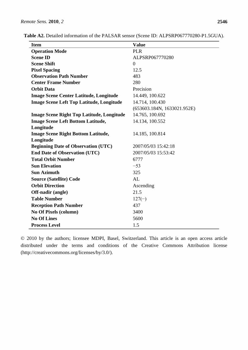
Ayutthaya provincial boundary. Table A2, in the Appendix, shows detailed information for the

PALSAR sensor. Prior to use in the current study, radiometric calibration had been applied to the

PALSAR product at Level 1.5, defined in the PALSAR product specifications by JAXA as

normalizing all pixels using the cosine of the incidence angle.

Figure 4. ALOS/PALSAR image (Scene ID: ALPSRP067770280-P1.5GUA), with back

scattering in the HH, HV,VH and VV polarization, overlaid with highways (red) and the

Ayutthaya provincial boundary (white).


2538

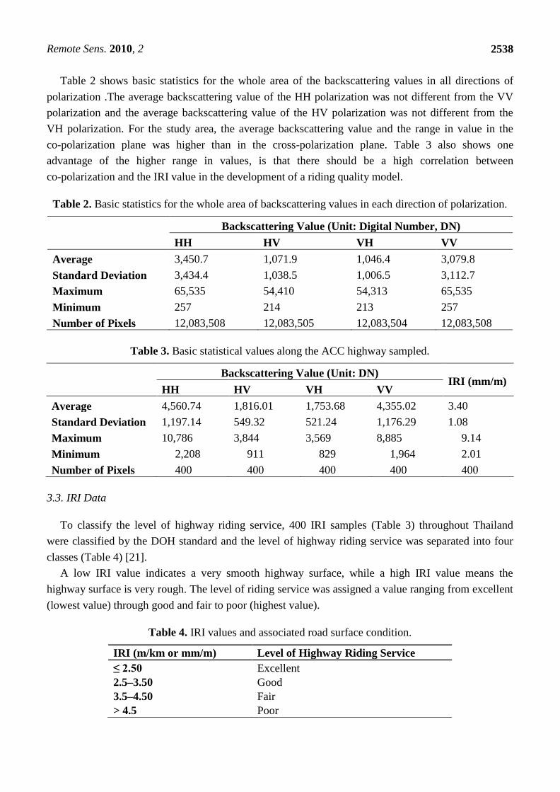
Table 2 shows basic statistics for the whole area of the backscattering values in all directions of

polarization .The average backscattering value of the HH polarization was not different from the VV

polarization and the average backscattering value of the HV polarization was not different from the

VH polarization. For the study area, the average backscattering value and the range in value in the

co-polarization plane was higher than in the cross-polarization plane. Table 3 also shows one

advantage of the higher range in values, is that there should be a high correlation between

co-polarization and the IRI value in the development of a riding quality model.

Table 2. Basic statistics for the whole area of backscattering values in each direction of polarization.

Backscattering Value (Unit: Digital Number, DN)

HH HV VH VV

Average 3,450.7 1,071.9 1,046.4 3,079.8

Standard Deviation 3,434.4 1,038.5 1,006.5 3,112.7

Maximum 65,535 54,410 54,313 65,535

Minimum 257 214 213 257

Number of Pixels 12,083,508 12,083,505 12,083,504 12,083,508

Table 3. Basic statistical values along the ACC highway sampled.

Backscattering Value (Unit: DN)

IRI (mm/m) HH HV VH VV

Average 4,560.74 1,816.01 1,753.68 4,355.02 3.40

Standard Deviation 1,197.14 549.32 521.24 1,176.29 1.08

Maximum 10,786 3,844 3,569 8,885 9.14

Minimum 2,208 911 829 1,964 2.01

Number of Pixels 400 400 400 400 400

3.3. IRI Data

To classify the level of highway riding service, 400 IRI samples (Table 3) throughout Thailand

were classified by the DOH standard and the level of highway riding service was separated into four

classes (Table 4) [21].

A low IRI value indicates a very smooth highway surface, while a high IRI value means the

highway surface is very rough. The level of riding service was assigned a value ranging from excellent

(lowest value) through good and fair to poor (highest value).

Table 4. IRI values and associated road surface condition.

IRI (m/km or mm/m) Level of Highway Riding Service

≤ 2.50 Excellent

2.5–3.50 Good

3.5–4.50 Fair

> 4.5 Poor


2539

4. Results and Model Explanation

4.1. Multinomial Logit Model

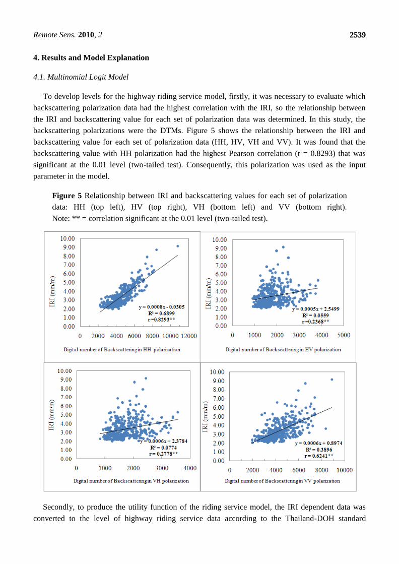
To develop levels for the highway riding service model, firstly, it was necessary to evaluate which

backscattering polarization data had the highest correlation with the IRI, so the relationship between

the IRI and backscattering value for each set of polarization data was determined. In this study, the

backscattering polarizations were the DTMs. Figure 5 shows the relationship between the IRI and

backscattering value for each set of polarization data (HH, HV, VH and VV). It was found that the

backscattering value with HH polarization had the highest Pearson correlation (r = 0.8293) that was

significant at the 0.01 level (two-tailed test). Consequently, this polarization was used as the input

parameter in the model.

Figure 5 Relationship between IRI and backscattering values for each set of polarization

data: HH (top left), HV (top right), VH (bottom left) and VV (bottom right).

Note: ** = correlation significant at the 0.01 level (two-tailed test).

Secondly, to produce the utility function of the riding service model, the IRI dependent data was

converted to the level of highway riding service data according to the Thailand-DOH standard


2540

(Table 4). Consequently, the qualities in the riding service estimation model were constructed using

Equations 1–3, with the reference category being the poor condition. This model was significant at the

0.01 level (two-tailed test), the global test for the constant variable (0) tested the null hypothesis that

0 = 0 and variable DNHH tested the null hypothesis that DNHH = 0. All variables in Equations 1–3

were significant at the 0.01 level with student’s t-test (two-tail).

HRQfair|poor = 8.7302 − 0.0015DNHH (1)

(t = 5.40) (t = −5.20)

HRQgood|poor = 21.0454 − 0.0039DNHH (2)

(t = 9.85) (t = −9.65)

HRQexcellent|poor = 25.4662 − 0.0053DNHH (3)

(t = 10.99) (t = −11.28)

(2 = 0.36,

2 =364.86, df = 3, p = 0.00)

where: DNHH is the digital number of HH polarization; HRQfair|poor is the highway riding quality

of service of the fair condition with reference to the poor condition; HRQgood|poor is the highway

riding quality of service of the good condition with reference to the poor condition; and

HRQexcellent|poor is the highway riding quality of service of the excellent condition with reference to

the poor condition.

Using the riding quality model developed, it was possible to determine the probability of

selecting the level of riding service using Equations 4–6, with the reference category being the poor

condition:

Pfair 𝐷𝑁𝐻𝐻 = 1

1+exp [−8.7302 +0.0015𝐷𝑁𝐻𝐻 ] (4)

Pgood 𝐷𝑁𝐻𝐻 = 1

1+exp [−21.0454 +0.0039𝐷𝑁𝐻𝐻 ] (5)

Pexcellent 𝐷𝑁𝐻𝐻 = 1

1+exp [−25.4662 +0.0053𝐷𝑁𝐻𝐻] (6)

The probability of selecting the poor riding service could be determined by using Equation 7:

Ppoor 𝐷𝑁𝐻𝐻 = 1 − Pfair 𝐷𝑁𝐻𝐻 −Pgood 𝐷𝑁𝐻𝐻 −Pexcellent 𝐷𝑁𝐻𝐻 (7)

The decision criteria to select the level of highway riding service model were provided using

Equation 8:

𝐿𝐻𝑅 =

poor, Ppoor 𝐷𝑁𝐻𝐻 > Pfair 𝐷𝑁𝐻𝐻 , Pgood 𝐷𝑁𝐻𝐻 , Pexcellent 𝐷𝑁𝐻𝐻

fair, Pfair 𝐷𝑁𝐻𝐻 > Ppoor 𝐷𝑁𝐻𝐻 , Pgood 𝐷𝑁𝐻𝐻 , Pexcellent 𝐷𝑁𝐻𝐻

good, Pgood 𝐷𝑁𝐻𝐻 > Ppoor 𝐷𝑁𝐻𝐻 , Pgood 𝐷𝑁𝐻𝐻 , Pexcellent 𝐷𝑁𝐻𝐻

excellent, Pexcellent 𝐷𝑁𝐻𝐻 > Ppoor 𝐷𝑁𝐻𝐻 , Pfair 𝐷𝑁𝐻𝐻 , Pgood 𝐷𝑁𝐻𝐻

(8)

where: LHR is the level of riding service; Ppoor(DNHH) is the probability number of HH

polarization of the poor condition; Pfair(DNHH) is the probability number of HH polarization of the

fair condition; Pgood(DNHH) is the probability number of HH polarization of the good condition;

and Pexcellent(DNHH) is the probability number of HH polarization of the excellent condition.


2541

Table 5 shows the classification results obtained using the level of riding service model

(multinomial logit model). Validation of this model indicated that the model was only 61.00% correct.

Consequently, a binary logit model was developed.

Table 5. Classification results using the first level of riding quality model (multinomial logit model).

Observed Predicted Percent

Correct Fair Poor Good Excellent

Fair 32 20 6 0 55.17

Poor 11 46 27 0 54.76

Good 2 19 145 17 79.23

Excellent 0 0 54 21 18.00

Overall percentage 11.25 21.25 58.00 9.50 61.00

4.2. Binary Logit Model

Binary logit model was developed by reclassifying the level of riding service into two groups,

namely good, if the IRI value was less than or equal to 3.5 mm/m, otherwise the quality was classified

as poor. The new quality of riding service estimation model was constructed as Equation 9. This model

was significant at the 0.01 level (two-tailed test), the variable 0 and variable DNHH were significant

at the 0.01 level with student’s t-test (two-tail).

HRQgood|poor = 14.4799 − 0.0029 DNHH (9)

(t = 9.87) (t = −9.69)

(2 = 0.54,

2 = 279.39, df = 1, p = 0.00)

where: DNHH is the digital number of the HH polarization; HRQ good|poor is the highway riding

quality of service of the good condition with the reference category being the poor condition.

Using this riding quality model, the probability to select the level of riding service could be

determined as shown in Equation 10 (the reference category is the poor condition). The decision

criteria to select the level of highway riding service model were provided using Equation 11:

Pgood 𝐷𝑁𝐻𝐻 = 1

1+exp [−14.4799+0.0029 𝐷𝑁𝐻𝐻] (10)

𝐿𝐻𝑅 = good, Pgood 𝐷𝑁𝐻𝐻 ≥ 0.50

poor, Pgood 𝐷𝑁𝐻𝐻 < 0.50 (11)

Table 6 shows validation of the binary logit function, after substitution of the digital number (DN)

value into the logit model indicated that the model had an accuracy assessment of prediction of the

highway level of service equal to 87.00% (using data from highway numbers 32, 309, 347 and 3063).

Table 6. Classification results using the second level of riding quality model (binary logit model).

Observed Predicted

Percent Correct Poor Good

Poor 112 30 78.87

Good 22 236 91.47

Overall percentage 33.50 66.50 87.00


2542

The marginal effect of decision criteria to select good riding service was derived from the partial

derivative of Equation 10 and was calculated using Equation 12. A unit increase in the DNHH value

decreased the probability of selecting the good level by 0.00289.

∂Pgood 𝐷𝑁𝐻𝐻𝑖

∂𝐷𝑁𝐻𝐻𝑖 = 0.0029(

−1

1+exp [−14.4799+0.0029 𝐷𝑁𝐻𝐻i ]) (12)

Figure 6 shows the relationship between backscattering and the probability of selection of

highway service level being good. From the probability function of the binary logit model, if the

DNHH value is greater than or equal to 4,946 (14.2445/0.00288), then the riding service will be poor.

With reference to the marginal effect, it was concluded that if the DNHH value increased further, then

the level of riding service would become very poor.

Figure 6. Relationship between backscattering and probability of selection of

highway service level = good.

The application of a binary logit model to highway number 3467, involved substitution of the

backscattering value (100 samples) into the model for the probability of selecting the good condition,

which resulted in the accuracy assessment for the prediction of the highway level of service being

97.00% (Table 7).

Table 7. Classification results using the level of riding quality model of highway number 3467

(100 samples).

Observed Predicted

Percent Correct Poor Good

Poor 12 2 85.71

Good 1 85 1.16

Overall percentage 12.00 85.00 97.00

Figure 7 shows the relationship between backscattering and the probability of selection of

highway number 3467 with service level equal to good. It can be concluded that if the


2543

backscattering value is approximately more than 5,000, then the level of pavement service will

be poor.

Figure 7. Relationship between backscattering and the probability of selecting highway

number 3467 with service level = good.

5. Discussion and Conclusion

A new approach was proposed to determine the level of highway riding service using the binary

logit model. After the back substitution of DNHH in this function, the accuracy of the approach was

87.00%. The analysis showed that an increase in the backscattering value for copolarization, in either

the HH or VV polarization, indicated a poor condition of the pavement surface. It was concluded that

the most suitable variable for developing riding quality evaluation was the backscattering value of the

HH polarization. From the probability function of the binary logit model, if the DNHH value were

greater than or equal to 4,946 (14.2445/0.00288), then the riding quality would be poor. From the

marginal effect function of the binary logit model, if the DNHH value were to increase further, then

the level of riding service would become very poor. The models developed were applied to analyze

highway number 3467 (100 samples) to demonstrate the capability of each model. It was found that the

accuracy assessment for the prediction of the highway level of service equaled 97.00%.

Since only one set of ALOS/PALSAR images (during 3–7 May 2007) was used in this study, and as

this is a preliminary study of the proposed technique, more intensive investigation must be carried out

using ALOS/PALSAR images in various seasons.

In future, satellite data resolution may be finer than 12.50 m, for example, down to a resolution of

3 m, so that the accuracy would be greater than in this analysis and an automatic technique could be

applied. Because the PALSAR resolution was only 12.5 m and the IRI data, on average, was only

about 25.0 m, the current study used an average of two pixels of PALSAR resolution. In further

studies, it should be possible to record the IRI value to be less than or equal to the PALSAR resolution.

The current study developed the relationship between IRI and satellite data in terms of a mathematical

model. Further study should be carried out to develop a physical properties model to explain

this relationship.


2544

Acknowledgements

The authors thank Wanchai Parkluck, the Deputy Director General of the Department of Highways,

Thailand, for providing the IRI data and acknowledge the support of the Japan Aerospace Exploration

Agency (JAXA) in providing the PALSAR data.

References and Notes

1. Grote, K.; Hubbard, S.; Harvey J.; Rubin, Y. Evaluation of infiltration in layered pavements using

surface GPR reflection techniques. J. Appl. Geophys. 2005, 57, 129-153.

2. Wang, H. Road Profiler Performance Evaluation and Accuracy Criteria Analysis; Virginia

Polytechnic Institute and State University: Blacksburg, VA, USA, 2006; p. 73.

3. Sayers, M.W.; Karamihas, S.M. The Little Book of Profiling—Basic Information about Measuring

and Interpreting Road Profiles; University of Michigan: Ann Arbor, MI, USA, 1998; p. 102.

4. Mactutis, J.A.; Alavi, S.H.; Ott, W.C. Investigation of relationship between roughness and

pavement surface distress based on WesTrack project. Transp. Res. Rec. 2000, 1699, 107-113.

5. Baus, R.; Hong, W. Investigation and Evaluation of Roadway Rideability Equipment and

Specifications; Report FHWA-SC-99-05; Federal Highway Administration/South Carolina

Department of Transportation: Columbia, SC, USA, 1999.

6. Ksaibati, K.; McNamera, R.; Miley, W.; Armaghani, J. Pavement roughness data collection and

utilization. Transp. Res. Rec. 1999, 1655, 86-92.

7. Kelly, L.S.; Leslie, T.G.; Lynn, D.E. Pavement Smoothness Index Relationships: Final Report;

Publication No. FHWA-RD-02-057; Turner-Fairbank Highway Research Center, Federal

Highway Administration, Research, Development, and Technology, U.S. Department of

Transportation: McLean, VA, USA, 2002.

8. Benedetto, A.; Pensa, S. Indirect diagnosis of pavement structural damages using surface GPR

reflection techniques. J. Appl. Geophys. 2007, 62, 107-123.

9. Dashevsky, Y.A.; Dashevsky, O.Y.; Filkovsky, M.I.; Synakh, V.S. Capacitance sounding: A new

geophysical method for asphalt pavement quality evaluation. J. Appl. Geophys. 2005, 57, 95-106.

10. Simonsen, E.; Isacsson, U. Thaw weakening of pavement structures in cold regions. Cold Reg.

Sci. Technol. 1999, 29, 135-151.

11. Terzi, S. Modeling the pavement serviceability ratio of flexible highway pavements by artificial

neural networks. Constr. Build. Mater. 2007, 21, 590-593.

12. Bergmeister, K.; Santa, U. Road Surface Monitoring and Pavement Analysis; ASECAP: Pula,

Croatia, 2006; pp. 283-288.

13. Saarenketo, T.; Scullion, T. Road evaluation with ground penetrating radar. J. Appl. Geophys.

2000, 43, 119-138.

14. Shresthaa, R.L.; Cartera, W.E.; Sartoria, M.; Luzuma, B.J.; Slatton, K.C. Airborne laser swath

mapping: Quantifying changes in sandy beaches over time scales of weeks to years. ISPRS J.

Photogramm. Remote Sens. 2005, 59, 222-232.

15. Alam, J.B.; Nahar, T.; Shaha, B. Evaluation of national highway by geographical information

system. Int. J. Environ. Res. 2008, 2, 365-370.


2545

16. Hans, Z.; Ryan, T.; Shauna, H.; Reg, S.; Sitansu, P. Use of LiDAR-Based elevation data for

highway drainage analysis: A qualitative assessment. In Proceedings of the 2003 Mid-Continent

Transportation Research Symposium, Ames, IA, USA, August 2003.

17. Stevens, L.B. Road Surface Management for Local Governments—Resource Notebook;

Publication No. DOT-I-85-37; Federal Highway Administration: Washington, DC, USA, May

1985.

18. JAXA. Advanced land observing satellite website. Available online: http://www.alos-restec.jp/

aboutalos_e.html (accessed on 15 May 2008).

19. Transportation Research Board (TRB). Special Report 209: Highway Capacity Manual, 3rd ed.;

National Research Council: Washington, DC, USA, 2000.

20. DOH. Department of Highways, Thailand Website. Available online: http://www.doh.go.th/

index_doh.aspx (accessed on 31 May 2007).

21. McFadden, D. Conditional logit analysis of qualitative choice behavior. In Frontiers in

Econometrics; Zarembka, P., Ed.; Academic Press: New York, NY, USA, 1973.

Appendix

Table A1. Details of the PALSAR system [18].

Mode Fine ScanSAR Polarimetric

(Experimental mode)

Center Frequency 1270 MHz (L band)

Chirp Bandwidth 28MHz 14MHz 14MHz 28MHz 14MHz

Polarization HH or VV HH+HV Or

VV+VH

HH or VV HH+HV+VH+VV

Incident angle 8 to 60° 18 to 43° 18 to 43° 8 to 30°

Range Resolution 7 to 44 m 14 to 88 m 100 m (multi-look) 24 to 89 m

Observation

Swath

40 to 70

km

40 to 70 km 250 to 350 km 20 to 65 km

Bit Length 5 bits 5 bits 5 bits 3 or 5 bits

Data rate 240

Mbps

240 Mbps 120 Mbps, 240

Mbps

240 Mbps

NE sigma zero < −23 dB (swath width 70 km) < −25 dB < −29 dB

< −25 dB (swath width 60 km)

S/A < −16 dB (Swath width 70 km) > 21 dB > 19 dB

< −21 dB (Swath width 60 km)

Radiometric

accuracy Scene: 1 dB / Orbit: 1.5 dB


2546

Table A2. Detailed information of the PALSAR sensor (Scene ID: ALPSRP067770280-P1.5GUA).

Item Value

Operation Mode PLR

Scene ID ALPSRP067770280

Scene Shift 0

Pixel Spacing 12.5

Observation Path Number 483

Center Frame Number 280

Orbit Data Precision

Image Scene Center Latitude, Longitude 14.449, 100.622

Image Scene Left Top Latitude, Longitude 14.714, 100.430

(653603.184N, 1633021.952E)

Image Scene Right Top Latitude, Longitude 14.765, 100.692

Image Scene Left Bottom Latitude,

Longitude

14.134, 100.552

Image Scene Right Bottom Latitude,

Longitude

14.185, 100.814

Beginning Date of Observation (UTC) 2007/05/03 15:42:18

End Date of Observation (UTC) 2007/05/03 15:53:42

Total Orbit Number 6777

Sun Elevation −53

Sun Azimuth 325

Source (Satellite) Code AL

Orbit Direction Ascending

Off-nadir (angle) 21.5

Table Number 127(−)

Reception Path Number 437

No Of Pixels (column) 3400

No Of Lines 5600

Process Level 1.5

© 2010 by the authors; licensee MDPI, Basel, Switzerland. This article is an open access article

distributed under the terms and conditions of the Creative Commons Attribution license

(http://creativecommons.org/licenses/by/3.0/).

riding quality model for asphalt pavement monitoring using

Documents