richardson’s extrapolation - university of washingtongreenbau/math_498/lecture04... ·...
TRANSCRIPT

Richardson’s Extrapolation
Tim Chartier and Anne Greenbaum
Department of Mathematics @
Winter 2008
Tim Chartier and Anne Greenbaum Richardson’s Extrapolation

Approximating the Second Derivative
From last time, we derived that:
f ′′(x) ≈f (x + h) − 2f (x) + f (x − h)
h2
the truncation error is O(h2).
Further, rounding error analysis predicts rounding errors ofsize about ǫ/h2.
Therefore, the smallest total error occurs when h is aboutǫ1/4 and then the truncation error and the rounding errorare each about
√ǫ.
With machine precision ǫ ≈ 10−16, this means that hshould not be taken to be less than about 10−4.
Tim Chartier and Anne Greenbaum Richardson’s Extrapolation
Numerical Derivatives on MATLAB
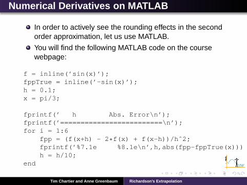
In order to actively see the rounding effects in the secondorder approximation, let us use MATLAB.
You will find the following MATLAB code on the coursewebpage:
f = inline(’sin(x)’);fppTrue = inline(’-sin(x)’);h = 0.1;x = pi/3;
fprintf(’ h Abs. Error\n’);fprintf(’=========================\n’);for i = 1:6
fpp = (f(x+h) - 2 * f(x) + f(x-h))/hˆ2;fprintf(’%7.1e %8.1e\n’,h,abs(fpp-fppTrue(x)))h = h/10;
end
Tim Chartier and Anne Greenbaum Richardson’s Extrapolation

Rounding errors in action
This MATLAB code produces the following table:
h Abs. Error=========================1.0e-001 7.2e-0041.0e-002 7.2e-0061.0e-003 7.2e-0081.0e-004 3.2e-0091.0e-005 3.7e-0071.0e-006 5.1e-005
Tim Chartier and Anne Greenbaum Richardson’s Extrapolation
Your Turn
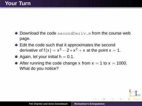
Download the code secondDeriv.m from the course webpage.
Edit the code such that it approximates the secondderivative of f (x) = x3 − 2 ∗ x2 + x at the point x = 1.
Again, let your initial h = 0.1.
After running the code change x from x = 1 to x = 1000.What do you notice?
Tim Chartier and Anne Greenbaum Richardson’s Extrapolation

Rounding errors again
Your code should have changed the inline functions to thefollowing:
f = inline(’xˆ3 - 2 * xˆ2 + x’);fppTrue = inline(’6 * x - 4’);
This MATLAB code produces the following table:
h Abs. Error=========================1.0e-001 7.2e-0041.0e-002 7.2e-0061.0e-003 7.2e-0081.0e-004 3.2e-0091.0e-005 3.7e-0071.0e-006 5.1e-005
How small h can be depends on the size of x .
Tim Chartier and Anne Greenbaum Richardson’s Extrapolation

Recognizing Error Behavior
Last time we also saw that Taylor Series of f about thepoint x and evaluated at x + h and x − h leads to thecentral difference formula:
f ′(x) =f (x + h) − f (x − h)
2h−
h2
6f ′′′(x0) −
h4
120f (5)(x0) − · · · .
This formula describes precisely how the error behaves.
This information can be exploited to improve the quality ofthe numerical solution without ever knowing f ′′′, f (5), . . ..
Recall that we have a O(h2) approximation.
Tim Chartier and Anne Greenbaum Richardson’s Extrapolation
Exploiting Knowledge of Higher Order Terms
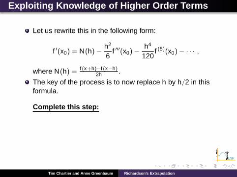
Let us rewrite this in the following form:
f ′(x0) = N(h) −h2
6f ′′′(x0) −
h4
120f (5)(x0) − · · · ,
where N(h) = f (x+h)−f (x−h)2h .
The key of the process is to now replace h by h/2 in thisformula.
Complete this step:
Tim Chartier and Anne Greenbaum Richardson’s Extrapolation

Canceling Higher Order Terms
Therefore, you find
f ′(x0) = N(
h2
)
−h2
24f ′′′(x0) −
h4
1920f (5)(x0) − · · · .
Look closely at what we had from before:
f ′(x0) = N(h) −h2
6f ′′′(x0) −
h4
120f (5)(x0) − · · · .
Careful substraction cancels a higher order term.
4f ′(x0) = 4N(
h2
)
− 4 h2
24 f ′′′(x0) − 4 h4
1920 f (5)(x0) − · · ·
−f ′(x0) = −N(h) + h2
6 f ′′′(x0) + h4
120 f (5)(x0) + · · ·
3f ′(x0) = 4N(
h2
)
− N(h) + h4
160 f (5)(x0) + · · ·
Tim Chartier and Anne Greenbaum Richardson’s Extrapolation

A Higher Order Method
Thus,
f ′(x0) = N(
h2
)
+N(h/2) − N(h)
3+
h4
160f (5)(x0) + · · ·
is a O(h4) formula.
Notice what we have done. We took two O(h2)approximations and created a O(h4) approximation.
We did require, however, that we have functionalevaluations at h and h/2.
Tim Chartier and Anne Greenbaum Richardson’s Extrapolation
Further observations
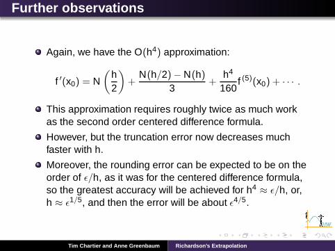
Again, we have the O(h4) approximation:
f ′(x0) = N(
h2
)
+N(h/2) − N(h)
3+
h4
160f (5)(x0) + · · · .
This approximation requires roughly twice as much workas the second order centered difference formula.
However, but the truncation error now decreases muchfaster with h.
Moreover, the rounding error can be expected to be on theorder of ǫ/h, as it was for the centered difference formula,so the greatest accuracy will be achieved for h4 ≈ ǫ/h, or,h ≈ ǫ1/5, and then the error will be about ǫ4/5.
Tim Chartier and Anne Greenbaum Richardson’s Extrapolation

Example
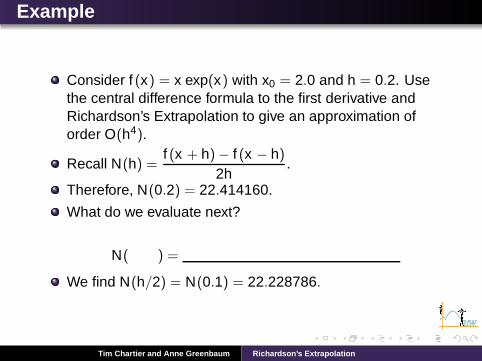
Consider f (x) = x exp(x) with x0 = 2.0 and h = 0.2. Usethe central difference formula to the first derivative andRichardson’s Extrapolation to give an approximation oforder O(h4).
Recall N(h) =f (x + h) − f (x − h)
2h.
Therefore, N(0.2) = 22.414160.
What do we evaluate next?
N( ) =
Tim Chartier and Anne Greenbaum Richardson’s Extrapolation
Example
Consider f (x) = x exp(x) with x0 = 2.0 and h = 0.2. Usethe central difference formula to the first derivative andRichardson’s Extrapolation to give an approximation oforder O(h4).
Recall N(h) =f (x + h) − f (x − h)
2h.
Therefore, N(0.2) = 22.414160.
What do we evaluate next?
N( ) =
We find N(h/2) = N(0.1) = 22.228786.
Tim Chartier and Anne Greenbaum Richardson’s Extrapolation

Example cont.
Therefore, our higher order approximation is
Tim Chartier and Anne Greenbaum Richardson’s Extrapolation

Example cont.
Therefore, our higher order approximation is
In particular, we find the approximation:
f ′(x0) = N(
h2
)
+N(h/2) − N(h)
3
= N(0.1) +N(0.1) − N(0.2)
3= 22.1670.
Note, f ′(x) = x exp(x) + exp(x), so f ′(x) = 22.1671 to fourdecimal places.
You should find that from approximations that contain zerodecimal places of accuracy we attain an approximationwith two decimal places of accuracy with truncation.
Tim Chartier and Anne Greenbaum Richardson’s Extrapolation

Richardson’s Extrapolation
This process is known as Richardson’s Extrapolation.
More generally, assume we have a formula N(h) thatapproximates an unknown value M and that
M − N(h) = K1h + K2h2 + K3h3 + · · · ,for some unknown constants K1, K2, K3, . . .. Note that inthis example, the truncation error is O(h).
Without knowing K1, K2, K3, . . . it is possible to produce ahigher order approximation as seen in our previousexample.
Note, we could use our result from the previous example toproduce an approximation of order O(h6). To understandthis statement more, let us look at an example.
Tim Chartier and Anne Greenbaum Richardson’s Extrapolation
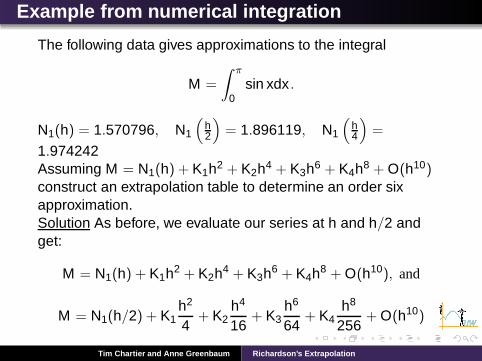
Example from numerical integration
The following data gives approximations to the integral
M =
∫ π
0sin xdx .
N1(h) = 1.570796, N1
(
h2
)
= 1.896119, N1
(
h4
)
=
1.974242Assuming M = N1(h) + K1h2 + K2h4 + K3h6 + K4h8 + O(h10)construct an extrapolation table to determine an order sixapproximation.Solution As before, we evaluate our series at h and h/2 andget:
M = N1(h) + K1h2 + K2h4 + K3h6 + K4h8 + O(h10), and
M = N1(h/2) + K1h2
4+ K2
h4
16+ K3
h6
64+ K4
h8
256+ O(h10)
Tim Chartier and Anne Greenbaum Richardson’s Extrapolation
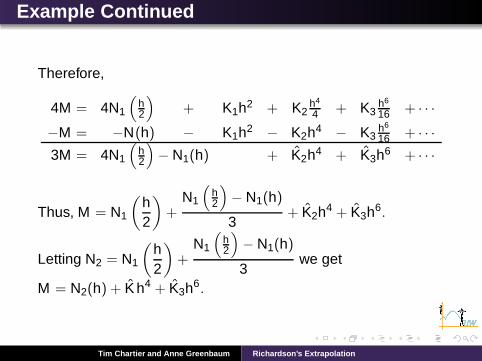
Example Continued
Therefore,
4M = 4N1
(
h2
)
+ K1h2 + K2h4
4 + K3h6
16 + · · ·
−M = −N(h) − K1h2 − K2h4 − K3h6
16 + · · ·
3M = 4N1
(
h2
)
− N1(h) + K̂2h4 + K̂3h6 + · · ·
Thus, M = N1
(
h2
)
+N1
(
h2
)
− N1(h)
3+ K̂2h4 + K̂3h6.
Letting N2 = N1
(
h2
)
+N1
(
h2
)
− N1(h)
3we get
M = N2(h) + K̂ h4 + K̂3h6.
Tim Chartier and Anne Greenbaum Richardson’s Extrapolation
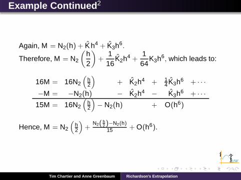
Example Continued2
Again, M = N2(h) + K̂ h4 + K̂3h6.
Therefore, M = N2
(
h2
)
+116
K̂2h4 +164
K3h6, which leads to:
16M = 16N2
(
h2
)
+ K̂2h4 + 14 K̂3h6 + · · ·
−M = −N2(h) − K̂2h4 − K̂3h6 + · · ·
15M = 16N2
(
h2
)
− N2(h) + O(h6)
Hence, M = N2
(
h2
)
+N2( h
2)−N2(h)
15 + O(h6).
Tim Chartier and Anne Greenbaum Richardson’s Extrapolation
Example Continued3
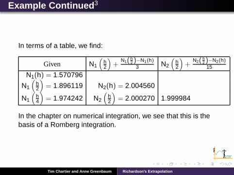
In terms of a table, we find:
Given N1
(
h2
)
+N1( h
2 )−N1(h)
3 N2
(
h2
)
+N2( h
2 )−N2(h)
15
N1(h) = 1.570796
N1
(
h2
)
= 1.896119 N2(h) = 2.004560
N1
(
h4
)
= 1.974242 N2
(
h2
)
= 2.000270 1.999984
In the chapter on numerical integration, we see that this is thebasis of a Romberg integration.
Tim Chartier and Anne Greenbaum Richardson’s Extrapolation

Example summary
Take a moment and reflect on the process we just followed.
We began with O(h2) approximations for which we knewthe Taylor expansion.
We used our O(h2) approximations to find N2 which wereorder O(h4) and again for which we knew the Taylorexpansions.
Finally, we used the N2 approximations to find an O(h6)approximation.
Could we continue this to find an order 8 approximation? Itdepends – remember that reducing h can lead to round-offerror. As long as we don’t hit that threshold, then ourcomputations do not corrupt our Taylor expansion.
Tim Chartier and Anne Greenbaum Richardson’s Extrapolation