rhinoceros - home - moos 3d services & training · robert mcneel & associates 1 1...
TRANSCRIPT

RH50-TM-L2-Aug-2013
Rhinoceros®
modeling tools for designers
Training Manual
Level 2


Robert McNeel & Associates i
Rhinoceros v5.0, Level 2, Training Manual
Revised 8/7/2013, Jerry Hambly
© Robert McNeel & Associates 2013
All Rights Reserved.
Printed in USA
Copyright © by Robert McNeel & Associates
Permission to make digital or hard copies of part or all of this work for personal or classroom use is granted without fee provided that copies are not made or distributed for profit or commercial advantage. To copy otherwise, to republish, to post on servers, or to redistribute to lists requires prior specific permission. Request permission to republish from Publications, Robert McNeel & Associates, 3670 Woodland Park Avenue
North, Seattle, WA 98103; FAX (206) 545-7321; e-mail [email protected].


Robert McNeel & Associates i i i
Table of Contents
PART I: Getting Started ..................................................... 5
1 Introduction ............................................................... 1
Duration ....................................................................... 1
Prerequisites: .............................................................. 1
Course Objectives ....................................................... 1
Schedule A: 3 Classroom Days ............................. 3
Schedule B: 6 Half Days (On-line Training) ........... 3
PART II: Interface Customization ...................................... 7
2 Customizing Rhino .................................................... 9
The toolbar layout ........................................................ 9
Rules for commands in buttons ............................ 15
Command aliases ...................................................... 18
Macro editor .............................................................. 19
Shortcut keys............................................................. 20
Plug-ins ..................................................................... 21
Scripting .................................................................... 24
Template files ............................................................ 25
PART III: Advanced Modeling Techniques ..................... 31
3 NURBS topology ..................................................... 33
4 Curve creation and continuity ................................ 37
Curve degree............................................................. 37
Curve and surface continuity ..................................... 39
Curve continuity and curvature graph ........................ 40
Advanced techniques for controlling continuity ......... 49
5 Surface continuity ................................................... 51
Analyzing surface continuity ...................................... 51
Matching surface continuity ....................................... 51
Add knots to control surface matching ...................... 55
Surfacing commands that pay attention to continuity 58
Surface blend options ................................................ 69
Fillets, blends and corners ........................................ 70
6 Modeling with history.............................................. 79
Activating history ....................................................... 80
Why is history off by default? ............................... 80
Steps in the History chain .......................................... 80
History enabled commands ....................................... 82
History-related commands ........................................ 82
7 Advanced surfacing techniques ............................ 85
Dome-shaped buttons ............................................... 85
Creased surfaces ...................................................... 91
Curve fairing to control surface quality ...................... 97
8 Use background bitmaps ...................................... 103
9 An approach to modeling ..................................... 111
10 Applying 2-D graphics ........................................... 121
Make a model from a 2-D drawing ........................... 126
11 Surface analysis .................................................... 131
12 Sculpting ................................................................ 137
Tools to help in control point editing ........................ 137
Gumball .............................................................. 137
DragMode .......................................................... 137
Nudge ................................................................. 138
SetPt .................................................................. 138
InsertKnot ........................................................... 138
InsertControlPoint............................................... 138
13 Deformation tools .................................................. 145
Deforming objects .................................................... 145
14 Blocks ..................................................................... 151
Instances and definitions ......................................... 151
Defining blocks ................................................... 151
Insertion points ................................................... 151
Embedded and linked blocks ............................. 151
Layers and blocks .................................................... 151
Editing blocks .......................................................... 152
15 Troubleshooting .................................................... 155
General strategy ...................................................... 155
Start with a clean file ............................................... 155
Guidelines for Repairing Files .................................. 155
16 Polygon meshes .................................................... 159
Render meshes ....................................................... 159
Meshes for manufacturing ....................................... 159
Meshes from NURBS objects .................................. 160
PART IV: Rendering ...................................................... 165
17 Rendering ............................................................... 167
Rendering properties ............................................... 169
Scene lighting .......................................................... 171
Image and bump maps ............................................ 173
Decals...................................................................... 174

Robert McNeel & Associates iv
List of Exercises
Exercise 1—Trackball mouse (warm-up).............................. 5
Exercise 2—Customizing Rhino’s interface .......................... 9
Exercise 3—Topology ........................................................ 33
Exercise 4—Trimmed NURBS ........................................... 35
Exercise 5—Curve degree ................................................. 37
Exercise 6—Geometric continuity ...................................... 43
Exercise 7—Tangent continuity .......................................... 45
Exercise 8—Curvature continuity ....................................... 48
Exercise 9—Surface continuityand ..................................... 51
Exercise 10—Continuity commands ................................... 58
Exercise 11—Patch options ............................................... 61
Exercise 12—Lofting .......................................................... 62
Exercise 13—Blends .......................................................... 63
Exercise 14—Blend options ............................................... 69
Exercise 15—Variable radius fillets .................................... 71
Exercise 16—Variable radius blends and chamfers ........... 72
Exercise 17—Fillet with patch ............................................ 73
Exercise 18—Soft corners .................................................. 73
Exercise 19—History introduction ...................................... 79
Exercise 20—Soft domed buttons ...................................... 85
Exercise 21—Surfaces with a crease ................................. 91
Exercise 22—Surfaces with a crease (Part 2) .................... 94
Exercise 23—Handset ...................................................... 103
Exercise 24—Cutout ........................................................ 111
Exercise 25—Importing an Adobe Illustrator file ............... 121
Exercise 26—Flow the logo onto a freeform surface with history ........................................................................ 123
Exercise 27—Making a detergent bottle ........................... 126
Exercise 28—Surface analysis ......................................... 131
Exercise 29—Dashboard.................................................. 139
Exercise 30—Using cage editing to deform an object ...... 145
Exercise 31—Using other deformation tools .................... 148
Exercise 32—Block basics ............................................... 152
Exercise 33—Inserting files as blocks .............................. 154
Exercise 34—Troubleshooting ......................................... 157
Exercise 35—Meshing...................................................... 159
Exercise 36—Rhino rendering .......................................... 167
Exercise 37—Rendering a scene ..................................... 169

PART I: Getting Started


Robert McNeel & Associates 1
1 Introduction This course guide accompanies the Level 2 training sessions in Rhinoceros. This course is designed for individuals who will be using and/or supporting Rhino.
The course explores advanced techniques in modeling to help participants better understand how to apply Rhino’s modeling tools in practical situations.
In class, you will receive information at an accelerated pace. For best results, practice at a Rhino workstation
between class sessions, and consult the Rhino Help system from the Help menu: Help Topics.
Duration
3 days
Prerequisites:
Completion of Level 1 training, plus three months’ experience using Rhino.
Course Objectives
In Level 2, you learn how to:
Customize toolbars and toolbar collections
Create simple macros
Use advanced object snaps
Use distance and angle constraints with object snaps
Construct and modify curves that will be used in surface building using control point editing methods
Evaluate curves using the curvature graph
Use a range of strategies to build surfaces
Rebuild surfaces and curves
Control surface curvature continuity
Create, manipulate, save and restore custom construction planes
Create surfaces and features using custom construction planes
Group objects
Visualize, evaluate, and analyze models utilizing shading features
Place text around an object or on a surface
Map planar curves to a surface
Create 3-D models from 2-D drawings and scanned images
Clean up imported files and export clean files
Use rendering tools


C H A P T E R 1 I N T R O D U C T I O N
Robert McNeel & Associates 3
Schedule A: 3 Classroom Days
Day 1 Topic
8-9:30 AM Introduction and warm up exercise.
9:30 AM-12PM Interface and customization
12-1PM Lunch
1-2:30 PM NURBS topology and curve degree
2:30 -5PM Curve and surface continuity
Day 2 Topic
8-10AM History, advanced surfacing and CPlane tools
10AM-12PM More CPlanes, mapping objects to surfaces
12-1PM Lunch
1-2:30PM Surface analysis
2:30 -5PM Putting it all together—Scoop exercise
Day 3 Topic
8-10AM More CPlanes, mapping objects to surfaces
10AM-12PM Surface analysis, direct surface manipulation
12-1PM Lunch
1-3PM Blocks, troubleshooting, Meshing
3 -5PM Rendering (time allowing)
Schedule B: 6 Half Days (On-line Training)
Session 1 Topic
9-10:45AM Introduction and warm up exercise.
11 AM-12:30PM Interface and customization
Session 2 Topic
9-10:45AM NURBS topology and curve degree
11AM-12:45PM Curve and surface continuity
Session 3 Topic
9-10:45AM History, advanced surfacing and CPlane tools
11AM-12:45PM More CPlanes, mapping objects to surfaces
Session 4 Topic
9-10:45AM Surface analysis
11AM-12:45PM Putting it all together—Scoop exercise
Session 5 Topic
9-10:45AM More CPlanes, mapping objects to surfaces
11AM-12:45PM Surface analysis, direct surface manipulation
Session 6 Topic
9-10:45AM Blocks, troubleshooting, Meshing
11AM-12:45PM Rendering (time allowing)


C H A P T E R 1 I N T R O D U C T I O N
Robert McNeel & Associates 5
Exercise 1—Trackball mouse (warm-up)
1 Begin a new model, save it as Trackball.3dm.
2 Model a trackball mouse on your own.
The dimensions are in millimeters. Use the dimensions as guides only.


PART II: Interface Customization


Robert McNeel & Associates 9
2 Customizing Rhino This chapter discusses customizing Rhino’s interface with the following tools:
Toolbar layout
Macro Editor
Shortcut keys
Scripting
Template files
The toolbar layout
The toolbar layout is the arrangement of toolbars containing command buttons on the screen. The toolbar layout is stored in a file with the .rui extension that you can open and save. Rui files contain command macros, icons in three sizes, as well as tooltips and button text. Rhino comes with a default toolbar file and automatically saves the active toolbar layout before closing unless the .rui file is read-only. You can create your own custom toolbar files and save them for later use.
You can have more than one toolbar file open at a time. This allows greater flexibility to display toolbars for particular tasks.
Rhino’s customization tools make it easy to create and modify toolbars and buttons. Adding to the flexibility is the ability to combine commands into macros to accomplish tasks that are more complex. In addition to toolbar customization, it is possible to set up command aliases and shortcut keys to accomplish tasks in Rhino.
Exercise 2—Customizing Rhino’s interface
In this exercise, we will create buttons, toolbars, macros, aliases, and shortcut keys that will be available to use throughout the class.
To create a custom toolbar collection
There are times that the standard commands and buttons do not do exactly what you want. For example, Zoom Extents will look at all of the objects in a model and then zoom to the extents of these objects. In this exercise, we will open a model that has several objects including some light objects.
Let us say we want to use Zoom Extents to zoom to the objects, but we do not want the command to consider the light objects. In this exercise, we will make a new toolbar with a button that will Zoom Extents while ignoring any light objects in the model.
1 Open the model ZoomLights.3dm.
2 From the Tools menu, click Toolbar Layout.
This opens the Rhino Options dialog on the Toolbars page.

C H A P T E R 2 C U S T O M I Z I N G R H I N O
Robert McNeel & Associates 10
3 Highlight the Default toolbar file.
4 On the Toolbars page click the File menu, click Save As.
5 Type Level 2 Training in the File name box and click Save.
A copy of the current default toolbar file is saved with the new name.
Toolbar files are saved with a .rui extension. You will use this new toolbar file to do some customization.

C H A P T E R 2 C U S T O M I Z I N G R H I N O
Robert McNeel & Associates 11
In the Rhino Options dialog, on the Toolbars page, all the open toolbar files are listed along with a list of all the individual toolbars for the selected toolbar file.
Check boxes show the current state of the toolbars. A checked box indicates that the toolbar is displayed.
To create a new toolbar
1 On the Toolbars page click the Edit menu, click New Toolbar.
2 In the Toolbars Properties dialog, name the toolbar Zoom, and click OK.
A new single button toolbar appears.

C H A P T E R 2 C U S T O M I Z I N G R H I N O
Robert McNeel & Associates 12
3 Close the Rhino Options dialog.
Another way to work with toolbars is to use the title bar of a floating toolbar.
4 Right-click on the title bar of the new toolbar you created.
A popup list of toolbar options and commands displays.
To edit the new button
1 Hold down the Shift key and right-click the smiley face button in the new toolbar.
The Button Editor dialog appears with fields for commands for the left and right mouse buttons, as well as for the tooltips.
2 In the Button Editor dialog, click Image only.
In the Text box, type Zoom No Lights.

C H A P T E R 2 C U S T O M I Z I N G R H I N O
Robert McNeel & Associates 13
3 For the Left mouse button Tooltip, type Zoom Extents except lights, for the Right mouse button tooltip, type Zoom Extents except lights all viewports.
4 In the Left Mouse Button Command box, type ! _SetRedrawOff _SelNone _SelLight _Invert _Zoom _Selected _SelNone _SetRedrawOn.
5 In the Right Mouse Button Command box, type ! _SetRedrawOff _SelNone _SelLight _Invert _Zoom _All _Selected _SelNone _SetRedrawOn.

C H A P T E R 2 C U S T O M I Z I N G R H I N O
Robert McNeel & Associates 14
To change the bitmap image for the button
1 In the Button Editor dialog, click the Edit... next to the button icon in the upper
right to open the Bitmap Editor.
The bitmap editor is a simple paint program that allows editing of the icon bitmap. It includes a grab function for capturing icon-sized pieces of the screen, and an import file function.
2 In the Edit Bitmap dialog, click the File
menu, click Import Bitmap to Fit, and select the ZoomNoLights_32.bmp.
You can import any bitmap image. If the bitmap is too large, it will be scaled to fit as it is imported.
3 In the Edit Bitmap dialog, make any changes to the picture, and click OK.
Double-click on the color swatches to the right of the standard color bar to access the Select Color dialog for more color
choices.
4 Click OK in the Button Editor dialog.

C H A P T E R 2 C U S T O M I Z I N G R H I N O
Robert McNeel & Associates 15
To change the bitmap image to use an alpha channel
Notice that the new button’s background color does not match the background color of the other buttons. We will change the image background using an alpha channel, so that it matches the Windows 3D Objects color like the
other buttons.
1 Hold down the Shift key and right-click the ZoomNoLights button.
2 In the Button Editor dialog, click Edit to open the Bitmap Editor.
3 Left click the upper right color swatch to the
right of the black color. Change the alpha color number, labeled A, for the button color from 255 to 1.
This will make the current paint color transparent.
4 Change to the Fill tool, then right-click in
the background area of the button image.
5 Click OK in the Edit Bitmap dialog, and then click OK in the Button Editor dialog.
The color matches the Windows 3D Objects color.
To use the new button
1 Click the ZoomNoLights button.
2 Use the button to zoom the model two ways.
You will notice that it ignores the lights when doing a Zoom Extents.
Rules for commands in buttons
You can enter the commands or command combinations in the appropriate boxes, using these rules:
Item Sample Description
Space !_Line A space is interpreted as Enter.
Commands do not have spaces (for example, SelLight) but you must leave a space between commands.
“ ‟ If your command string refers to a file, toolbar, layer, object name, or directory for
which the path includes spaces, the path, toolbar name, or directory location must be enclosed in double-quotes.
! (Exclamation mark) !-_circle An ! (Exclamation mark) followed by a space is interpreted as Cancel. Generally, it is best to begin a button command with an exclamation mark (!) if you want to cancel any other command that may be running when you click the button.
' (apostrophe) View manipulation commands like Zoom can be run in the middle of other
commands. For example, you can zoom and pan while picking curves for a loft. An '(apostrophe) prior to the command name indicates that the next command is a nest able command.

C H A P T E R 2 C U S T O M I Z I N G R H I N O
Robert McNeel & Associates 16
Item Sample Description
_ (underscore) An underscore (_) runs a command as an English command name.
Rhino can be localized in many languages. The non-English versions will have commands, prompts, command options, dialogs, menus, etc., translated into their respective languages. English commands will not work in these versions. For macros written in English to work on all computers (regardless of the language of Rhino), the macros need to force Rhino to interpret all commands as English command names, by using the underscore.
- (Hyphen) -_Sweep2 Commands with dialogs can be run at the command line with command line options.
To suppress the dialog and use command line options, prefix the command name with a hyphen (-).
Pause User input and screen picks are allowed in a macro by putting the Pause command in the macro. Commands that use dialogs, such as Revolve, do not accept input to the
dialogs from macros. Use the hyphen form of the command (-Revolve) to suppress the dialog and control it entirely from a macro.
Note: These rules also apply to scripts run using the ReadCommandFile command and pasting text at the
command prompt. More sophisticated scripting is possible with the Rhino Script plug-in, but quite a lot can
be done with the basic commands and macro rules.
Some very useful commands for macros are SelLast, SelPrev, SelName, Group, SetGroupName, SelGroup, Invert, SelAll, SelNone, ReadCommandFile, and SetWorkingDirectory.
To link a toolbar to a button
1 Shift+right-click the Zoom Extents button in the Standard toolbar.
2 In the Button Editor dialog, click in the Linked toolbar area, select Zoom from the list, and click OK.
Now the Zoom Extents button has a small black triangle in the lower right corner indicating it has a linked toolbar.
3 Click and hold the Zoom Extents button to fly out your newly created single button toolbar.
If you close the Zoom toolbar you just created, you can always re-open it using the linked button.

C H A P T E R 2 C U S T O M I Z I N G R H I N O
Robert McNeel & Associates 17
4 Try the new linked button.
To add a command to an existing button
1 Hold the Shift key and right-click the Move button on the Main toolbar.
2 In the Button Editor dialog, in the Right Mouse Button Command box, type ! _Move _Pause _Vertical
3 In the Edit Toolbar Button dialog, in the Right Tooltip box, type Move Vertical.
This button will allow you to duplicate objects in the same location. We will use this command several times
during the class.
4 Select one of the objects in the model and right-click on the Move button.

C H A P T E R 2 C U S T O M I Z I N G R H I N O
Robert McNeel & Associates 18
5 Move the selected object vertically from the construction plane.
Command aliases
The same commands and macros that are available for buttons are also available for command aliases. Command aliases are like using shorthand in Rhino. They are commands and macros that are activated whenever commands are allowed, but are often used as a keyboard shortcut followed by Enter, Spacebar or clicking the right mouse button.
Use aliases for command sequences that you use often or frequently.
Note: When making aliases, use keys that are close to each other or repeat the same character 2 or 3 times, so
they will be easy to use.
To make a command alias
1 Open the model Aliases.3dm.
2 From the Tools menu, click Options.
3 In the Rhino Options dialog, on the Aliases page, you can add aliases and command strings or macros.

C H A P T E R 2 C U S T O M I Z I N G R H I N O
Robert McNeel & Associates 19
4 Click New to make a new alias.
We will make aliases to mirror selected objects vertically and horizontally across the origin of the active construction plane. These are handy when making symmetrical objects built centered on the origin.
5 In the Alias column, type mx.
In the Command Macro column, type ! _Mirror _Pause _XAxis
The alias is in the left column and the command string or macro is in the right column. The same rules apply here as with the buttons. Aliases can be used within other aliases' macros or button macros.
6 Click New to make another new alias.
7 In the Alias column, type my.
In the Command Macro column, type ! _Mirror _Pause _YAxis.
To try the new aliases
Select some geometry and type mx or my and press Enter.
If no objects are pre-selected, the Pause in the script prompts you to select objects, and an Enter will complete the selection set.
Macro editor
When making macros that are more complicated, it is good practice to use Rhino’s built-in macro editor. Macros can be edited and run directly from the editor. This allows you to quickly test whether command options and syntax are correct.

C H A P T E R 2 C U S T O M I Z I N G R H I N O
Robert McNeel & Associates 20
To use the macro editor
In the following example we will make a mirror macro that allows you to mirror across the construction plane. We will use the macro editor to build and test the macro before we add it to the Alias list.
1 From the Tools menu, click Command, then click Macro Editor.
2 In the macro editor type ! _Mirror _Pause _3Point 0 1,0,0 0,1,0.
3 To test the macro, click the Run icon in the macro editor.
4 If the macro runs as expected, select the text and copy it to
the clipboard.
5 Open the Options dialog on the Alias page and make a new alias mc. Paste the text from the macro editor into the alias command column.
6 Select some geometry and try the new alias out. Type mc and
press Enter.
To Export and Import Options
There are times when you might want to copy all or some of the options from one computer to another. An example might be a desktop computer and a laptop computer. This is especially true for aliases, keyboard shortcuts, and display modes. Rhino has commands that Export options to a file as well as Import options from a file.
1 From the Tools menu, click Export Options.
2 In the Save As dialog, for the File Name, type Level2_Options.
The current options are saved to a file.
3 Now, delete one of the aliases you previously made.
4 From the Tools menu, click Import Options.
5 In the Import Options dialog, select the file you just saved.
6 For the Options to import, click Aliases, Appearance, or any other options you wish to import.
Check to see if the alias you deleted is back.
Shortcut keys
The same commands, command strings, and macros that you can use for buttons and aliases are also available
for keyboard shortcuts. Shortcuts are commands and macros that are activated by certain combinations of function keys, Ctrl, Alt, and alphanumeric keys.
To make a shortcut key
1 From the Tools menu, click Options.
2 In the Rhino Options dialog, on the Keyboard page, you can add command strings or macros.
3 Click in the column next to the F4 to make a new shortcut.
4 Type _DisableObject snap _Toggle for the shortcut.
This shortcut will make it easy to toggle the state of running object snaps.

C H A P T E R 2 C U S T O M I Z I N G R H I N O
Robert McNeel & Associates 21
5 Close the dialog and try it out.
There are several shortcut keys that already have commands assigned. The same rules apply here as with the buttons and aliases.
Plug-ins
Plug-ins are programs that extend the functionality of Rhino. Plug-in classifications include:
Included plug-ins
Shipped and installed with Rhino. Some of these plug-ins are loaded, for example Rhino Render, Render Development Kit, Rhino Toolbars and Menus, BoxEdit, etc. Others are installed, but not loaded. Most of these plug-ins are Import/Export plug-ins. They are generally enabled and will get loaded when they are used for the
first time.
Rhino 5.0 Labs plug-ins
Experimental plug-ins developed in-house. These plug-ins are being considered for inclusion in future service releases or the next version of Rhino. They are available for download from the Rhino 5.0 Labs Tools website.
McNeel plug-ins
Flamingo nXt, Penguin, Brazil (rendering) and Bongo (animation) are McNeel products that are available for purchase.

C H A P T E R 2 C U S T O M I Z I N G R H I N O
Robert McNeel & Associates 22
Third-party plug-ins
These are programs and utilities that are developed by third-party developers. Some of these are free, but most are available for purchase. A few of the programs are stand-alone applications that work with Rhino, but
are not plug-ins. Generally, they add some specific capability to Rhino. For example RhinoCam is a CAM application, VRay is a rendering application, RhinoGold is jewelry design software, etc. For more information about these programs visit the Rhino Resources website.
To load a plug-in
For this example we have included a plug-in from the Rhino 5.0 labs page for you to install and use.
1 From the Tools menu, click Options.
2 Click Plug-ins.
A list of currently loaded and available plug-ins is displayed.
3 On the Plug-ins page, click Install.
4 In the Load Plug-In dialog, navigate to the Level 2/Models/Plug-ins folder, then, depending on which version of Rhino 5.0 you’re running, click either RhinoPolyhedra_x64.rhp or RhinoPolyhedra_x86.rhp (needed for 32-bit version of Rhino 5.0).
5 To run the command, type Polyhedron on the command line.

C H A P T E R 2 C U S T O M I Z I N G R H I N O
Robert McNeel & Associates 23
6 In the Polyhedron dialog, select one of the polyhedrons from the list, then click a center point and a radius point.
To load a plug-in using drag and drop
1 Open a Windows Explorer window.
2 Navigate to the folder that has the plug-in you want to install.
3 Simply click and hold the plug-in file, drag it and drop it into the Rhino window.

C H A P T E R 2 C U S T O M I Z I N G R H I N O
Robert McNeel & Associates 24
Scripting
Rhinoceros supports scripting using VBScript.
To script Rhino, you must have some programming skills. Fortunately, VBScript is simpler to program than many other languages, and there are materials available to help you get started. VBScript is a programming language developed and supported by Microsoft.
We will not cover how to write a script in this class, but we will learn how to run a script and apply it to a button.
The following script will list information about the current model.
To load a script
1 From the Tools menu, click RhinoScript, then click Load.
2 In the Load Script File dialog, click Add.
3 In the Open dialog, select CurrentModelInfo.rvb, then
click Open.
Note: You may get a message that Rhino “Cannot find
the script file CurrentModelInfo.rvb.
If that happens you will need to include the full path to the folder where the script file is located or add a search path in the Files section of Rhino Options.
4 In the Load Script File dialog, highlight
CurrentModelInfo.rvb, then click Load.
5 Save the current model. If you do not have a saved version of the model, no information is possible.
6 From the Tools menu, click RhinoScript, then click Run.
7 In the Run Script Subroutine dialog, click
CurrentModelInfo and then click OK.
A dialog describing the current information about this model displays.

C H A P T E R 2 C U S T O M I Z I N G R H I N O
Robert McNeel & Associates 25
To edit the script file
1 From the Tools menu, click RhinoScript, then click Edit.
2 On the Rhino Script Editor window, from the File menu, click Open.
3 On the Open dialog, select CurrentModelInfo.rvb, then click Open.
We will not be editing script files in this class. This exercise is to show how to access the editing feature if needed.
4 Close the Rhino Script Editor window.
To make a button that will load or run a script
1 From the Tools menu, click Toolbar Layout.
2 In the Toolbars dialog, check the File toolbar then close the dialog.
3 Right-click on the title bar of the File toolbar, then click New Button from the popup menu.
4 In the Button Editor dialog, in the Left Mouse Button Tooltip, type Current Model Information.
5 In the Right Tooltip, type Load Current Model Information.
6 In the Text box, type Model Info.
7 In the Left Mouse Button Command box, type ! -_RunScript (CurrentModelInfo)
8 In the Right Mouse Button Command box, type ! -_LoadScript “CurrentModelInfo.rvb”
To add a custom bitmap
1 In the Button Editor dialog, click Edit.
2 In the Edit Bitmap dialog, from the File menu, click Import Bitmap, and Open the
CurrentModelInfo.bmp, then click Open.
3 In the Button Editor dialog, click OK.
4 Try the new button.
Template files
A template is a Rhino model file you can use to store basic settings. Templates include all the information that is stored in a Rhino 3DM file: objects, blocks, layouts, grid settings, viewport layout, layers, units, tolerances, render settings, dimension settings, notes, and any setting in document properties.
You can use the default templates that are installed with Rhino or save your own templates to base future models on. You will likely want to have templates with specific characteristics needed for particular types of model
building.
The standard templates that come with Rhino have different viewport layouts or unit settings, but no geometry, and default settings for everything else. Different projects may require other settings to be changed. You can have templates with different settings for anything that can be saved in a model file, including render mesh, angle tolerance, named layers, lights, and standard pre-built geometry and notes.
If you include notes in your template, they will show in the Open Template File dialog.

C H A P T E R 2 C U S T O M I Z I N G R H I N O
Robert McNeel & Associates 26
The New command begins a new model with a template (optional). It will use the default template unless you change it to one of the other templates or to any other Rhino model file.
To change the template that opens by default when Rhino starts up, choose New and select the template file you
would like to open when Rhino starts, then check the Use this file when Rhino starts box.
To create a template
1 Start a new model.
2 Select the Small Objects - Inches.3dm file as the template.
3 From the Render menu, click Current Renderer, and then click Rhino Render.
To set the Document Properties
1 From the File menu, click Properties.
2 In the Document Properties dialog, on the Grid page, change the Snap spacing to 0.1, the Minor grid lines every to 0.1, the Major lines every to 10, and the Grid line count to 10.
3 On the Mesh page change the setting to Smooth and slower.

C H A P T E R 2 C U S T O M I Z I N G R H I N O
Robert McNeel & Associates 27
4 On the Rhino Render page, check Use lights on layers that are off.
5 On the Units page, change the Angle tolerance to 0.5, click OK.
The end tangent normals will be determined by this setting.
To set up the layers
1 Open the Layers panel and rename Layer 05 to Spotlights, Layer 04 to Curves, Layer 03 to Surfaces, and Default to Reference.
Make the Spotlights layer current.
Delete Layer 01 and Layer 02 layers.
2 Set up a spotlight so that it points at the origin and is approximately 45 degrees in the Top viewport and tilted 45 degrees in the Front viewport.

C H A P T E R 2 C U S T O M I Z I N G R H I N O
Robert McNeel & Associates 28
3 Use the my alias to mirror the light to make a second one.
4 To make the Curves layer the only visible layer, from the Edit menu, click Layers then click One Layer On. Select the Curves layer.
To set save notes
1 From the Panel menu, click Notes.
Type the details about this template in the Notes panel.
2 From the File menu, click Save As Template.
Name the template Small Objects –Decimal Inches - 0.001.3dm.
This file with all of its settings is now available any time you start a new model.
C H A P T E R 2 C U S T O M I Z I N G R H I N O
Robert McNeel & Associates 29
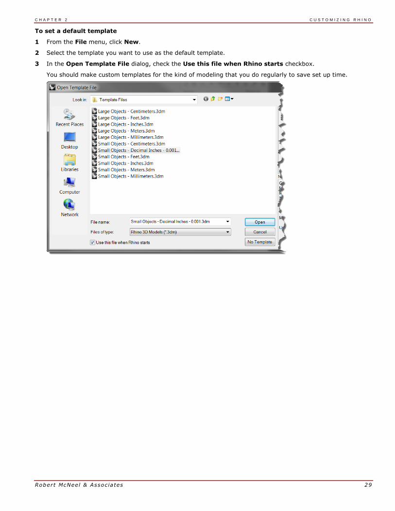
To set a default template
1 From the File menu, click New.
2 Select the template you want to use as the default template.
3 In the Open Template File dialog, check the Use this file when Rhino starts checkbox.
You should make custom templates for the kind of modeling that you do regularly to save set up time.

PART III: Advanced Modeling Techniques


Rober t McNeel & Assoc ia tes 33
3 NURBS topology The underlying geometry of NURBS surfaces have a rectangular topology in UV, or parameter space. Rows of surface points, and parameterization, are organized in two directions (U and V). These two directions are crosswise to each other, at more or less 90 degrees on an ideal surface, though this is not always possible. This structure is not always obvious when creating or manipulating a surface. Remembering this structure is useful in deciding which strategies to use when creating or editing geometry.
Exercise 3—Topology
This exercise will demonstrate how NURBS topology is organized and discuss some special cases that need
consideration when creating or editing geometry.
1 Open the model Topology.3dm.
There are several surfaces visible on the current layer.
2 Turn on the control points of the simple
rectangular plane on the left.
It has four control points, one at each corner—this is a simple untrimmed planar surface that shows the rectangular topology.
3 Now, turn on the control points of the, curvier surface.
There are many more points, but it is clear that they are arranged in a rectangular fashion.
1 Select the cylinder.
It appears as a continuous circular surface, but it also has a rectangular boundary.
2 Use the ShowEdges command (Analyze menu: Edge Tools > click Show Edges) to highlight the
surface edges.
Notice that there is a seam highlighted on the cylinder. The seam that is highlighted represents two edges of the rectangle, while the other two edges are circular at the top and the bottom. The rectangular topology is
present here, also.
3 Select the sphere.
It appears as a closed continuous object.
4 Use the ShowEdges command to highlight the
edges.
Notice that there is a seam highlighted on the sphere. The highlighted seam represents two edges of a rectangular NURBS surface, while the other two edges are collapsed to a single point at the poles. When all of the points of an untrimmed edge are collapsed into a single
point, it is called a singularity.
The rectangular topology is present here, also, though very distorted.

C H A P T E R 3 N U R B S T O P O L O G Y
Robert McNeel & Associates 34
1 Turn on the Control Points for the sphere.
2 Zoom Target (View menu: Zoom > Zoom Target)
draw a select window very tight around one of the poles of the sphere.
3 Select the point at one pole of the sphere and start the Smooth (Transform menu: Smooth) command.
4 In the Smooth dialog, uncheck Smooth Z, then click OK.
A hole appears at the pole of the sphere. There’s
no longer a singularity at this pole of the sphere. ShowEdges will highlight this as an edge as well.
5 Use the Home key to zoom back out.
This is the fastest way to step back through view changes.
To select points
1 Open the Select Points toolbar.
2 Select a single point at random on the sphere.
3 From the Select Points toolbar, click Select U.
An entire row of points is selected.
4 Clear the selection by clicking in an empty area and select another point on the sphere.
5 From the Select Points toolbar, click Select V.
A row of points in the other direction of the
rectangle is selected. This arrangement into u- and v-directions is always the case in NURBS surfaces.
6 Try the other buttons in this toolbar on your own.

C H A P T E R 3 N U R B S T O P O L O G Y
Robert McNeel & Associates 35
Exercise 4—Trimmed NURBS
1 Open the model Trimmed NURBS.3dm.
This surface has been trimmed out of a much larger surface. The underlying four sided surface data is still available after a surface has been trimmed, but it is limited by the trim curves (edges) on the surface.
2 Select the surface and turn on the control points, then drag a few control points.
Control points can be manipulated on the trimmed part of the surface or the rest of the surface, but notice that the trimming edges move around as the underlying surface changes. The trim curve always stays on the surface.
3 Use the Undo command to undo the point manipulation.
To remove the trims from a surface
1 Start the Untrim (Surface menu: Surface Edit Tools > Untrim) command.
2 Select the single edge of the trimmed surface.
The original underlying surface appears and the trim boundary disappears.
3 Use the Undo command to return to the previous trimmed surface.
To detach a trimming curve from a surface
1 Start the Untrim command with the KeepTrimObjects option set to Yes (Surface menu: Surface Edit Tools > Detach Trim).
2 Select the edge of the surface.
The original underlying surface appears. The boundary edges are converted to curves,
which are no longer associated with the surface.
3 Undo, to return to the previous trimmed
surface.

C H A P T E R 3 N U R B S T O P O L O G Y
Robert McNeel & Associates 36
To shrink a trimmed surface
1 Start the ShrinkTrimmedSrf command (Surface menu: Surface Edit Tools >
Shrink Trimmed Surface).
2 Select the surface and press Enter to end the command.
The underlying untrimmed surface is replaced by a one with a smaller range that matches the old surface exactly in that range. You will see no visible change in the trimmed surface. Only the underlying untrimmed surface is altered.

Rober t McNeel & Assoc ia tes 37
4 Curve creation and continuity We will begin this part of the course by reviewing a few concepts and techniques related to NURBS curves that will simplify the learning process during the rest of the class. Curve building techniques have a significant effect on the surfaces that you build from them.
Curve degree
The degree of a curve refers to the highest degree polynomial in the equation for the curve. In practice it relates to the extent of the influence a single control point has over the length of the curve.
For higher degree curves, a control point has less local influence and a more broad influence over the entire the length of the curve. It also has higher internal continuity.
In the example below, the five curves have their control points at the same six points. Each curve has a different
degree. The degree can be set with the Degree option in the Curve command.
Exercise 5—Curve degree
1 Open the model Curve Degree.3dm.
2 Use the Curve command (Curve menu: Free-Form > Control Points) with Degree set to 1, using the
Point object snap to snap to each of the points.
3 Repeat the Curve command with Degree set to 2.
Degree 1: Control points on curve—no bending.
Degree 2: Control points off curve.
4 Repeat the Curve command with
Degree set to 3.
5 Repeat the Curve command with Degree set to 4.
Degree 3
Degree 4
6 Repeat the Curve command with Degree set to 5.
Degree 5

C H A P T E R 4 C U R V E C R E A T I O N A N D C O N T I N U I T Y
Robert McNeel & Associates 38
Analyzing the curvature of a curve
1 Use the CurvatureGraph command (Analyze menu: Curve > Curvature Graph On) to turn on the
curvature graph for one of the curves. Set the DisplayScale to a number that shows the graph as in the illustration—between 110-120 should work
well.
The graph indicates the curvature on the curve—this is the inverse of the radius of curvature. The smaller the radius of curvature at any point on the curve, the larger the amount of curvature.
2 Turn on the control points for the curve you have graphed and view the curvature graph as you drag some control points. Note the change in the curvature hairs as you move points.
3 Repeat this process for each of the
curves. You can use the Curvature Graph dialog buttons to remove or add objects from the graph display.
Note:
Degree 1 curves have no curvature and no graph displays.
Degree 2 curves are internally continuous for tangency—the steps in the graph indicate this condition. Note that only the graph is stepped not the curve.
Degree 3 curves have continuous curvature—the graph will not show steps but may show hard peaks and valleys. Again, the curve is not kinked at these places—the graph shows an abrupt but not discontinuous change in curvature.
In higher degree curves, higher levels of continuity are possible.
For example, a Degree 4 curve is continuous in the rate of change of curvature—the graph doesn’t show
any hard peaks.
A Degree 5 curve is continuous in the rate of change of the rate of change of curvature. The graph doesn’t show any particular features for higher degree curves but it will tend to be smooth.
Changing the degree of the curve to a higher degree with the ChangeDegree command with Deformable=No will not improve the internal continuity, but lowering the degree will adversely affect the
continuity.
Rebuilding a curve with the Rebuild command will change the internal continuity.

C H A P T E R 4 C U R V E C R E A T I O N A N D C O N T I N U I T Y
Robert McNeel & Associates 39
Curve and surface continuity
Since creating a good surface so often depends upon the quality and continuity of the input curves, it is
worthwhile clarifying the concept of continuity among curves.
For most curve building and surface building purposes we can talk about four useful levels of continuity:
Not continuous
The curves or surfaces do not meet at their end points or edges. Where there is no continuity, the objects cannot be joined.
Positional continuity (G0)
Curves meet at their end points, surfaces meet at their edges.
Positional continuity means that there is a kink at the point where two curves
meet. The curves can be joined in Rhino into a single curve but there will be a kink and the curve can still be exploded into at least two sub-curves.
Similarly two surfaces may meet along a common edge but will show a kink or seam, a hard line between the surfaces. For practical purposes, only the end points of a curve or the last rows of points along the edges of two
untrimmed surfaces need to match to determine G0 continuity.
Tangency continuity (G1)
Curves or surfaces meet and the directions of the tangents at the endpoints or edges is the same. You
should not see a crease or a sharp edge.
Tangency is the direction of a curve at any particular point along the curve
Where two curves meet at their endpoints the tangency condition between them is determined by the direction in
which the curves are each heading exactly at their endpoints. If the directions are collinear, then the curves are considered tangent. There is no hard corner or kink where the two curves meet. This tangency direction is
controlled by the direction of the line between the end control point and the next control point on a curve.
In order for two curves to be tangent to one another, their endpoints must be coincident (G0) and the second control point on each curve must lie on a line passing through the curve endpoints. A total of four control points, two from each curve, must lie on this imaginary line.

C H A P T E R 4 C U R V E C R E A T I O N A N D C O N T I N U I T Y
Robert McNeel & Associates 40
Curvature continuity (G2)
Curves or surfaces meet, their tangent directions are the same and the radius
of curvature is the same for each at the end point.
Curvature Continuity includes the above G0 and G1 conditions and adds the further requirement that the radius of curvature be the same at the common endpoints of the two curves. Curvature continuity is the smoothest condition over which the user has any direct control, although smoother relationships are possible.
For example, G3 continuity means that not only are the conditions for G2 continuity met, but also that the rate of change of the curvature is the same on both curves or surfaces at the common end points or edges.
G4 means that the rate of change of the rate of change is the same. Rhino has tools to build such curves and surfaces, but fewer tools for checking and verifying such continuity than for G0-G2.
G5+ has no visible evidence of more continuity.
Curve continuity and curvature graph
Rhino has two analysis commands that will help illustrate the difference between curvature and tangency. In the following exercise, we will use the CurvatureGraph and the Curvature commands to gain a better understanding of tangent and curvature continuity.
To show continuity with a curvature graph
1 Open the model Curvature_Tangency.3dm.
There are five sets of curves, divided into three groups.
One group has positional (G0) continuity at their common ends.
Group (a-c) has tangency (G1) continuity at
their common ends.
C H A P T E R 4 C U R V E C R E A T I O N A N D C O N T I N U I T Y
Robert McNeel & Associates 41
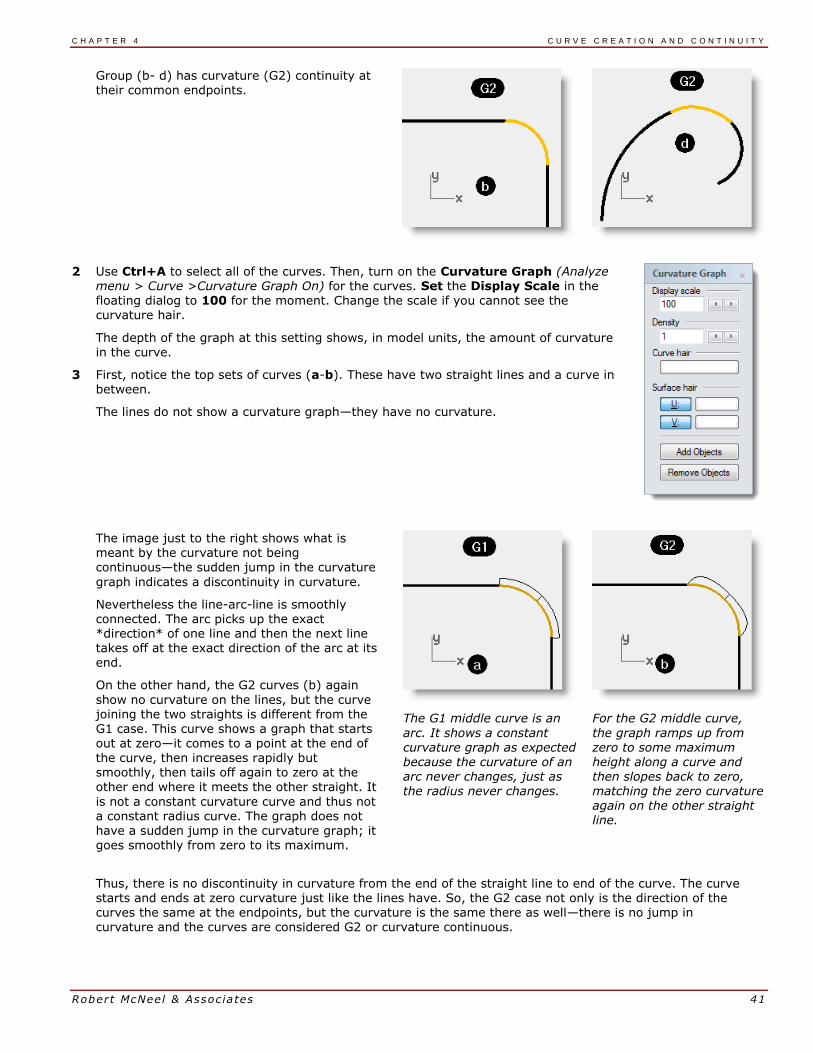
Group (b- d) has curvature (G2) continuity at their common endpoints.
2 Use Ctrl+A to select all of the curves. Then, turn on the Curvature Graph (Analyze menu > Curve >Curvature Graph On) for the curves. Set the Display Scale in the floating dialog to 100 for the moment. Change the scale if you cannot see the curvature hair.
The depth of the graph at this setting shows, in model units, the amount of curvature in the curve.
3 First, notice the top sets of curves (a-b). These have two straight lines and a curve in between.
The lines do not show a curvature graph—they have no curvature.
The image just to the right shows what is meant by the curvature not being
continuous—the sudden jump in the curvature
graph indicates a discontinuity in curvature.
Nevertheless the line-arc-line is smoothly connected. The arc picks up the exact *direction* of one line and then the next line takes off at the exact direction of the arc at its end.
On the other hand, the G2 curves (b) again
show no curvature on the lines, but the curve joining the two straights is different from the G1 case. This curve shows a graph that starts out at zero—it comes to a point at the end of the curve, then increases rapidly but smoothly, then tails off again to zero at the
other end where it meets the other straight. It
is not a constant curvature curve and thus not a constant radius curve. The graph does not have a sudden jump in the curvature graph; it goes smoothly from zero to its maximum.
The G1 middle curve is an
arc. It shows a constant curvature graph as expected because the curvature of an arc never changes, just as
the radius never changes.
For the G2 middle curve,
the graph ramps up from zero to some maximum height along a curve and then slopes back to zero,
matching the zero curvature again on the other straight line.
Thus, there is no discontinuity in curvature from the end of the straight line to end of the curve. The curve starts and ends at zero curvature just like the lines have. So, the G2 case not only is the direction of the curves the same at the endpoints, but the curvature is the same there as well—there is no jump in curvature and the curves are considered G2 or curvature continuous.

C H A P T E R 4 C U R V E C R E A T I O N A N D C O N T I N U I T Y
Robert McNeel & Associates 42
4 Next, look at the c and d curves.
These are also G1 and G2 but are not straight
lines so the graph shows up on all of the curves.
Again, the G1 set shows a step up or down in the graph at the common endpoints of the curves. This time the curve is not a constant arc—the graph shows that it increases in curvature out towards the middle.
On G2 curves, the graph for the middle curve shows the same height as the adjacent curves at the common endpoints—there are no abrupt steps in the graph.
The outer curve on the graph from one curve stays connected to the graph of the adjacent curve.
To show continuity with a curvature circle
1 Start the Curvature command (Analyze menu>Curvature circle) and select the middle curve in set c.
The circle that appears on the curve indicates the radius of curvature at that location—the circle that would result from the center and radius measured at that point on the curve.
2 Drag the circle along the curve.
Notice that where the circle is the smallest, the graph shows the largest amount of curvature. The curvature is the inverse of the radius at any point.
3 Click the MarkCurvature option on the command line.
Slide the circle, snap to an endpoint of the curve, and click to place a curvature circle.
4 Stop the command and restart it for the other curve sharing the endpoint just picked.
Place a circle on this endpoint as well.
The two circles have greatly different radii. Again, this indicates a
discontinuity in curvature. These curves are G1 / tangent only, so the curvature at the tangent meeting point is different for the two curves, and that is where the curvature graph would take a jump.
5 Repeat the same procedure to get circles at the ends of the curves in set d.
Notice that this time the circles from each curve at the common endpoint are
the same radius. These curves are curvature continuous.

C H A P T E R 4 C U R V E C R E A T I O N A N D C O N T I N U I T Y
Robert McNeel & Associates 43
6 Lastly, turn on the control points for the middle curves in c and d. Select the “middle” control
point on either curve and move it around.
Notice that while the curvature graph changes greatly, the continuity at each end with the adjacent curves is not affected.
The G1 curve graphs stay stepped, though, the size of the step changes.
The G2 curve graphs stay connected, although there is a peak that forms there.
7 Look at the graphs for the G0 curves.
Notice that there is a gap in the graph—this indicates that there is only G0 or positional continuity.
The curvature circles, on the common
endpoints of these two curves, are not only different radii, but they are also not tangent—
they cross each other. There is a discontinuity in direction at the ends.
Exercise 6—Geometric continuity
1 Open the model Curve Continuity.3dm.
The two curves are clearly not tangent. Verify this with the continuity checking command GCon.
2 Start the GCon command (Analyze menu: Curve > Geometric Continuity).
3 Click near the common ends (1 and 2) of each curve.
Rhino displays a message on the command line indicating the curves are out of tolerance—the endpoints of the two curves are not close enough to each other to be considered the same.
Curve end difference = 0.030 millimeters Radius of curvature difference = 126.531 millimeters Curvature direction difference in degrees = 10.277 Tangent difference in degrees = 10.277 Curve ends are out of tolerance.
Often, imported curves are often "out of tolerance" and need this kind of repair for accurate modeling.
C H A P T E R 4 C U R V E C R E A T I O N A N D C O N T I N U I T Y
Robert McNeel & Associates 44
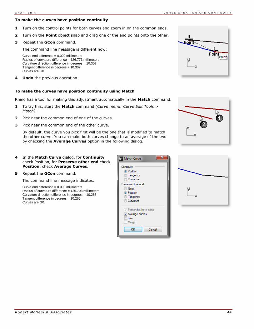
To make the curves have position continuity
1 Turn on the control points for both curves and zoom in on the common ends.
2 Turn on the Point object snap and drag one of the end points onto the other.
3 Repeat the GCon command.
The command line message is different now:
Curve end difference = 0.000 millimeters Radius of curvature difference = 126.771 millimeters Curvature direction difference in degrees = 10.307 Tangent difference in degrees = 10.307 Curves are G0.
4 Undo the previous operation.
To make the curves have position continuity using Match
Rhino has a tool for making this adjustment automatically in the Match command.
1 To try this, start the Match command (Curve menu: Curve Edit Tools > Match).
2 Pick near the common end of one of the curves.
3 Pick near the common end of the other curve.
By default, the curve you pick first will be the one that is modified to match the other curve. You can make both curves change to an average of the two by checking the Average Curves option in the following dialog.
4 In the Match Curve dialog, for Continuity check Position, for Preserve other end check Position, check Average Curves.
5 Repeat the GCon command.
The command line message indicates:
Curve end difference = 0.000 millimeters Radius of curvature difference = 126.708 millimeters Curvature direction difference in degrees = 10.265 Tangent difference in degrees = 10.265 Curves are G0.

C H A P T E R 4 C U R V E C R E A T I O N A N D C O N T I N U I T Y
Robert McNeel & Associates 45
Exercise 7—Tangent continuity
It is possible to establish a tangency (G1) condition between two curves by aligning the control points in a particular way. The endpoints at one end of the curves must be coincident and these points in addition to the next
point on each curve must fall in a line with each other. This can be done automatically with the Match command, although it is also easy to do by moving the control points using the normal Rhino transform commands.
We will use Move, SetPt, Rotate, Zoom Target, PointsOn (F10), PointsOff (F11) commands and the object snaps End, Point, Along, Between and the Tab lock to move the points in various ways to achieve tangency.
First, we will create some aliases that will be used in this exercise.
To make Along and Between aliases
Along and Between are one-time object snaps that are available in the Tools menu under Object snaps. They
can be used only after a command has been started and apply to only one pick. We will create new aliases for these object snaps.
1 In the Rhino Options dialog on the Aliases page, click the New button
2 In the Alias column, type a.
In the Command macro column, type _Along.
3 In the Alias column, type b.
4 In the Command macro column type _Between.
5 Close the Rhino Options dialog.
To change the continuity by adjusting control points using Rotate and the Tab direction lock
The tab direction lock locks the movement of the cursor when the tab key is pressed. It can be used for moving
objects, dragging, or curve and line creation.
To activate tab direction lock press and release the Tab when Rhino is asking for a location in space. The cursor will be constrained to a line between its location in space at the time the Tab key is pressed and the location in
space of the last clicked point.
When the direction is locked, it can be released with another press and release of the Tab, and a new, corrected direction set with yet another Tab press.
1 Turn on the control points for both curves.
2 Select the control point (1) second from the end of one of the curves.
3 Start the Rotate command (Transform menu: Rotate).
4 Using the Point object snap, select the common
endpoints (2) of the two curves for the Center of rotation.
5 For the First reference point, snap to the current location of the selected control point.

C H A P T E R 4 C U R V E C R E A T I O N A N D C O N T I N U I T Y
Robert McNeel & Associates 46
6 For the Second reference point, make sure the point object snap is still active. Hover the
cursor, but do not click, over the second point
(3) on the other curve. While the Point object snap flag is visible on screen, indicating the cursor is locked onto the control point, press and release the Tab key. Do not click with the mouse.
7 Bring the cursor back over to the other curve-- notice that the position is constrained to a line between the center of rotation and the second point on the second curve; that is, the location
of the cursor when you hit the tab key. You can
now click the mouse on the side opposite the second curve.
During rotation, the tab direction lock knows to make the line from the center and not from the first reference point.
The rotation endpoint will be exactly in line
with the center of rotation and the second point on the second curve.
To change the continuity by adjusting control points using the Between object snap
1 Use the OneLayerOn command to turn on only the 3D Curves layer.
2 Check the continuity of the curves with the GCon command.
3 Turn on the control points for both curves.
4 Window select the common endpoints of both curves (1).
5 Use the Move command (Transform menu:
Move) to move the points.
6 For the Point to move from snap to the same point (1).
7 For the Point to move to, type b and press
Enter to use the Between object snap.
8 For the First point, snap to the second point (2) on one curve.
9 For the Second point, snap to the second point (3) on the other curve.
The common points are moved in-between the two second points, aligning the four points.

C H A P T E R 4 C U R V E C R E A T I O N A N D C O N T I N U I T Y
Robert McNeel & Associates 47
10 Check the continuity.
To change the continuity by adjusting control points using the Along object snap
1 Undo the previous operation.
2 Select the second point (3) on the curve on the
right.
3 Use the Move command (Transform menu: Move) to move the point.
4 For the Point to move from, snap to the selected point.
5 For the Point to move to, type A and press Enter to use the Along object snap.
6 For the Start of tracking line, snap to the second point (2) on the other curve.
7 For the End of tracking line, snap to the common points (1).
The point tracks along a line that goes through the two points, aligning the four points.
8 Click to place the point.
9 Check the continuity.

C H A P T E R 4 C U R V E C R E A T I O N A N D C O N T I N U I T Y
Robert McNeel & Associates 48
To edit the curves without losing tangency continuity
With the Tab technique, we can adjust the meeting point of the curves, or the shape of either curve near the meeting point, without losing the G1 continuity.
1 Window select the common endpoints or select the second point on either curve.
Turn on the Point object snap and drag the point(s) to the next one of the four critical points.
2 When the Point object snap flag shows on the
screen, use the Tab direction lock by pressing and releasing the Tab key without releasing the mouse button.
3 Drag the point(s) and the tangency is
maintained since the drag direction is constrained to the Tab direction lock line.
4 Release the left mouse button at any point to place the point(s).
Note: To maintain G1 continuity make sure that any point manipulation of the critical four points takes place
along the line on which they all fall.
Once you have G1 continuity you can still edit the curves near their ends without losing continuity, using the Tab direction lock.
This technique only works after tangency has been established.
Exercise 8—Curvature continuity
Adjusting points to establish curvature continuity is not as straightforward as for tangency. Curvature at the end
of a curve is determined by the position of the last three points on the curve, and their relationships to one another are not as straightforward as it is for tangency.
To establish curvature or G2 continuity, the Match command is the only practical way in most cases.
To match the curves
1 Use the Match command (Curve menu: Curve Edit Tools > Match) to match the magenta (1)
curve to the red (2) curve. Set Continuity to Curvature, Preserve other end to Curvature, and uncheck Average curves.
When you use Match with Curvature checked on these particular curves, the third point on the curve to be changed is constrained to a
position calculated by Rhino to establish the desired continuity.

C H A P T E R 4 C U R V E C R E A T I O N A N D C O N T I N U I T Y
Robert McNeel & Associates 49
The curve being changed is significantly altered in shape.
Moving the third point by hand will break the G2 continuity at the ends, though G1 will be maintained
Advanced techniques for controlling continuity
There are two additional methods to edit curves while maintaining continuity in Rhino. (1) The EndBulge command constrains points at the end to maintain continuity with the adjacent curve. (2) Adding knots will allow
more flexibility when changing the curve's shape.
To edit the curve with end bulge
1 Right-click on the Copy button to make a duplicate of the magenta curve and then Lock it.
2 Start the EndBulge command (Edit menu: Adjust End Bulge).
3 Select the magenta curve.
Notice that there are more points displayed than were on the original curve.
The EndBulge command adds more control points to the curve if the curve has less than the required control point count.
4 Select the third point, drag it, and click to place the point, press Enter to end the command.
If the endpoint of the curve has G2 continuity with another curve, the G2 continuity will be
preserved, because EndBulge preserves the curvature at the endpoint of the curve.
Note: Adjusting control points will work to match curvature only in the simple case of matching to a straight line.

C H A P T E R 4 C U R V E C R E A T I O N A N D C O N T I N U I T Y
Robert McNeel & Associates 50
To add a knot
Adding a knot or two to the curve will put more points near the end so that the third point can be nearer the end. Knots are added to curves and surfaces with the InsertKnot command.
1 Undo your previous adjustments.
2 Start the InsertKnot command (Edit menu: Control Points > Insert Knot).
3 Select the magenta curve.
4 Pick a location on the curve to add a knot in between the first two knot markers.
In general, a curve or surface will tend to behave better in point editing if new knots are placed midway between existing knots, thus maintaining a uniform distribution.
Adding knots also results in added control points.
Knots and control points are not the same thing and the new control points will not be added at exactly the new knot location.
The Automatic option automatically inserts a new knot in each span exactly half way between existing knots."
If you only want to place knots in some of the spans, you should place
these individually by clicking on the desired locations along the curve.
Existing knots are highlighted in white.
5 Match the curves after inserting a knot into the magenta curve.
Inserting knots closer to the end of curves will change how much Match changes the curve.

Rober t McNeel & Assoc ia tes 51
5 Surface continuity The continuity characteristics for curves can also be also applied to surfaces. Instead of dealing with the endpoint, second, and third points, entire rows of points at the edge, and the next two positions away from the edge are involved. The tools for checking continuity between surfaces are different from the simple GCon command.
Analyzing surface continuity
Rhino takes advantage of the OpenGL display capability to create false color displays for checking curvature and continuity within and between surfaces. These tools are located in the Analyze menu, under Surface. The tool, which most directly measures G0-G2 continuity between surfaces, is the Zebra command. Zebra analysis simulates reflection of a striped background on the surface.
Note: An OpenGL graphics accelerator card is not necessary to use these tools, although they may work faster
with OpenGL acceleration.
Matching surface continuity
The command used to establish G0, G1 or G2 continuity between surfaces is the MatchSrf command.
Match surface options
Option Description
Average surfaces Both surfaces are modified to an intermediate shape.
Refine match Determines if the match results should be tested for accuracy and refined so
that the faces match to a specified tolerance.
Match edges by closest points
The surface being changed is aligned to the edge it is being matched to by pulling each edge point to the closest point on the other edge.
Preserve other end If the surface does not have enough points its degree is raised (up to a maximum of 5), until there are enough points.
Isocurve direction adjustment
Specifies the way the parameterization of the matched surfaces is determined.
Option Description
Automatic Evaluates the target edge, then uses Match target isocurve direction if it is an untrimmed edge or Make perpendicular to target edge if it is a trimmed edge.
Preserve isocurve direction As closely as possible, keeps the existing isocurve directions the same as
they were in the surface before matching.
Match target isocurve direction
Makes the isocurves of the surface that is being adjusted parallel to those of the surface it matches.
Make perpendicular to
target edge
Makes the isocurves of the surface that is being adjusted perpendicular to
the edge being matched.
Exercise 9—Surface continuity and MatchSrf
The MatchSrf command takes surface edges as input and modifies one or both of the surfaces. You need to tell
the command exactly which edge to change and then which edge to match to the target surface. We will match the white surface's edge to the green one first. Both the edge to change and the edge to match to are untrimmed on these surfaces.
While MatchSrf is generally used to adjust surfaces that are fairly close to being at the desired continuity, this example is somewhat exaggerated in order to clearly show the functionality and options.

C H A P T E R 5 S U R F A C E C O N T I N U I T Y
Robert McNeel & Associates 52
1 Open the model Surface Continuity.3dm.
2 Start the MatchSrf command (Surface menu: Surface Edit Tools >
Match).
3 Select the edge of the white surface on the edge nearest the green surface.
4 Select the edge of the green surface near the same location as the selection point on the white surface edge and press Enter.
5 In the Match Surface dialog, choose Position as the desired
Continuity, choose None for Preserve other end, uncheck Refine match, and choose Automatic for Isocurve direction adjustment.
Make sure all other check boxes are unchecked.
A shaded preview is automatically generated so you can see what the
result will be like.
6 Click OK.
The edge of the white surface is pulled over to match the edge of the green one.

C H A P T E R 5 S U R F A C E C O N T I N U I T Y
Robert McNeel & Associates 53
To check the continuity with Zebra analysis
1 Check the surfaces with Zebra analysis tool
(Analyze menu: Surface > Zebra).
This command relies on an approximation of the surface for its display information.
2 By default, the mesh generated by Zebra may be too coarse to get a good analysis of the surfaces. If the display shows very angular stripes rather than smooth stripes on each surface, click the Adjust
mesh button on the Zebra dialog.
In general, the analysis mesh should be much finer than the normal shade and render mesh meshes.
It is a good habit to set these meshes the first time you use a surface analysis display mode in a model. This
setting is then saved in the file.
3 Use the detailed controls to set mesh parameters.
For this type of mesh, it is often easiest to zero out (disable) the Maximum angle setting and rely entirely on the Minimum initial grid quads setting. This number can be quite high but may depend upon the geometry involved.
In this example, a setting here of 5000 to 10000 will generate a very fine and accurate mesh.
4 The analysis can be further improved by joining the surfaces to be tested. Join the two surfaces.
This will force a refinement of the mesh along the joined edge and help the Zebra stripes act more consistently.
There is no particular correlation between the stripes on one surface and the other except that they touch, indicating G0 continuity.

C H A P T E R 5 S U R F A C E C O N T I N U I T Y
Robert McNeel & Associates 54
5 Undo the Join.
To match the surface to tangency
1 Use the MatchSrf command (Surface menu: Surface Edit Tools > Match) again with the Tangency option for Continuity.
When you pick the edge to match you will get direction arrows that indicate which surface edge is being selected. The surface that the direction arrows are pointing toward is the surface whose edge is selected.
2 Check the surfaces with Zebra analysis. Rotate the view to view along the seam.
The ends of the stripes on each surface meet the ends on the other cleanly, though at an angle.
This indicates G1 continuity.
To match the surface to curvature
1 Use the MatchSrf command (Surface menu: Surface Edit Tools > Match) with the Curvature option.

C H A P T E R 5 S U R F A C E C O N T I N U I T Y
Robert McNeel & Associates 55
2 Check the surfaces with Zebra analysis.
The stripes now align themselves smoothly across the seam. Each stripe
connects smoothly to the counterpart on the other surface.
This indicates Curvature (G2) continuity.
Note: Doing these operations one after the other may yield different results than going straight to Curvature without first using Position. This is because each operation changes the surface near the edge, so the
next operation has a different starting surface.
Add knots to control surface matching
As in matching curves, MatchSrf will sometimes distort the surfaces more than is acceptable in order to attain the
desired continuity. We will add knots to surfaces to limit the influence of the MatchSrf operation. The new second and third rows of points will be closer to the edge of the surface.
Surfaces can also be adjusted with the EndBulge command.
To add a knot to a surface
1 Undo the previous operation.
2 Use the InsertKnot command (Edit menu: Control Points > Insert Knot) to insert a row of knots near the end of the white surface.
When this command is used on a surface, it has more options. You can choose to insert a row of knots in the U-direction, the V-direction,
or both. Choose Symmetrical to add knots at opposite ends of a surface.
3 Use MatchSrf to curvature match the surface to the other.
Notice that the new matched surface is different from the old one.
To adjust the surface using end bulge
The EndBulge command lets you edit the shape of a surface without changing the tangent direction and the curvature at the edge of the surface. This is useful when you need to alter the shape of a surface that has been matched to another surface.
EndBulge allows you to move control points at a specified location on the surface. These points are constrained along a path that keeps the direction and curvature from changing.
The surface can be adjusted equally along the entire selected edge or along a section of the edge. In the latter
case, the adjustment takes place at the specified point and tapers out to zero at either end of the range. Either the start or endpoint of the range can be coincident with the point to adjust, thus forcing the range to be entirely to one side of the adjustment point.

C H A P T E R 5 S U R F A C E C O N T I N U I T Y
Robert McNeel & Associates 56
1 Start the EndBulge command (Edit menu: Adjust End Bulge).
2 For the surface edge to adjust, pick the edge of the surface on the
right.
3 For the Point to edit, pick a point on the edge at which the actual adjustment will be controlled.
You can use object snaps and reference geometry to select a point with precision.
4 For the Start of region to edit, pick a point along the common edges to define the region to be adjusted.
5 For the End of region to edit, pick another point to define the region to
be adjusted.
To select a range at this point, slide the cursor along the edge and click at the beginning and endpoints of the range. If the whole edge is to be
adjusted equally, simply press Enter.
6 For the Point to adjust, select one of the points that are displayed.
Rhino shows three points, of which you are allowed to manipulate only two. When you move the second point, Rhino also moves the third
point that is not being directly manipulated in order to maintain the continuity. If you move the third
point it won’t change the second point
7 Drag the point and click to adjust the surface.
If maintaining the G2 curvature-matching condition at the edge is not needed, use the Continuity=Tangency
option to turn off one of the two points available for editing. Only G1 will be preserved.
8 Press Enter to end the command.

C H A P T E R 5 S U R F A C E C O N T I N U I T Y
Robert McNeel & Associates 57
To match an untrimmed surface to a trimmed surface
1 Start the MatchSrf command
(Surface menu: Surface Edit
Tools > Match).
2 Select the edge of the green surface on the edge nearest the blue surface.
The edge will not select and you will see the following message
on the command line:
Edge must be on the edge of a surface (not a trimmed edge). Select untrimmed surface edge to change ( MultipleMatches ).
3 Instead, select the untrimmed edge of the blue surface on the edge nearest the green surface.
4 Select the trimmed edge of the green surface near the same location as the selection point on the blue surface
edge.
5 In the Match Surface dialog, choose Curvature as the desired Continuity, choose None for Preserve other end, check Match edges by closest points,
and choose Automatic for Isocurve direction adjustment.
Make sure all other check boxes are unchecked.
A preview is automatically generated so you can see what the result will be like.
Notice that the blue surface does not include the entire untrimmed edge of the green surface. It only extends as far as the closest point from the original surface.

C H A P T E R 5 S U R F A C E C O N T I N U I T Y
Robert McNeel & Associates 58
6 In the Match Surface dialog, uncheck Match edges by closest
points, and check Refine match.
7 Change the Isocurve direction adjustment and the Preserve other end options to see what happens to the matched surface. When finished press OK.
Surfacing commands that pay attention to continuity
Rhino has several commands that that can build surfaces using the edges of other surfaces as input curves. They
can build the surfaces with G1 or G2 continuity to those neighboring surfaces. The commands are:
NetworkSrf
Sweep2
Patch (G1 only)
Loft (G1 only)
BlendSrf (G1 to G4)
The following exercises will provide a quick overview of these commands.
Exercise 10—Continuity commands
To create a surface from a network of curves
1 Open the model Continuity Commands.3dm.
On the Surfaces layer, two joined surfaces have been trimmed leaving a gap. This gap needs to be closed up with continuity to the surrounding surfaces.
2 Turn on the Network layer, if it is not already on, and make it current.
Several curves already in place define the required cross sections of the surface.
3 Use the NetworkSrf command (Surface menu: Curve Network) to close the hole with an untrimmed surface using the curves and the edges of the surfaces as input curves.

C H A P T E R 5 S U R F A C E C O N T I N U I T Y
Robert McNeel & Associates 59
4 For the Select curves in network, select the four edges that border the opening and the four curves inside the opening and press Enter.
Note that there is a maximum of four edge curves as input. You can also specify the tolerances or maximum deviation of the surface from the input curves.
By default, the edge tolerances are the same as the model's Absolute Tolerance setting. The interior curves' tolerance is set 10 times looser than that by default.
5 In the Surface From Curve Network dialog, choose Curvature continuity for all the edges, and click OK.
The surface that is created has
curvature continuity on all four
edges.
6 Check the resulting surface with Zebra analysis.
To make the surface with a two-rail sweep
1 Use the OneLayerOn command to open the Surfaces layer by itself again, and then click in the layers panel of the status bar, and select the Sweep2 layer.
2 Start the Sweep2 command (Surface
menu: Sweep 2 Rails) and select the long surface edges as the rails.
3 Select one short edge, the cross-section curves, and the other short edge as profiles.
4 Choose Curvature for both Rail curve options.
Since the rails are surface edges, the display labels the edges, and the
Sweep 2 Rails Options dialog gives the option of maintaining
continuity at these edges.
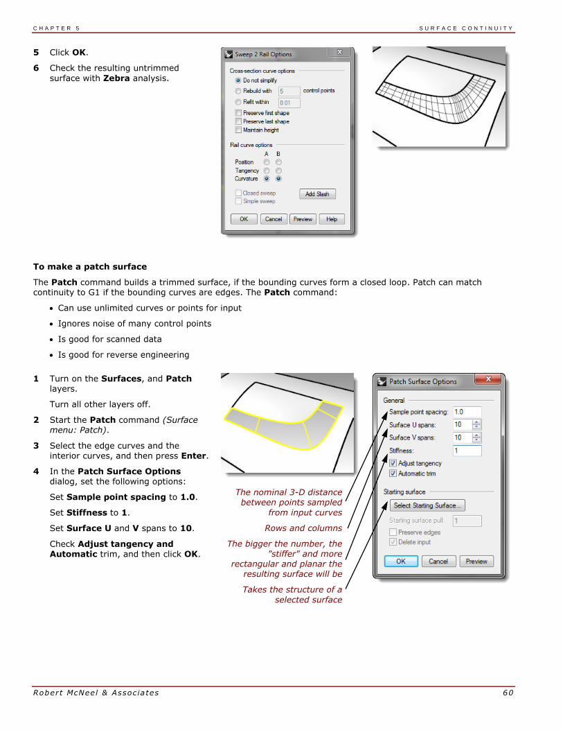
C H A P T E R 5 S U R F A C E C O N T I N U I T Y
Robert McNeel & Associates 60
5 Click OK.
6 Check the resulting untrimmed
surface with Zebra analysis.
To make a patch surface
The Patch command builds a trimmed surface, if the bounding curves form a closed loop. Patch can match continuity to G1 if the bounding curves are edges. The Patch command:
Can use unlimited curves or points for input
Ignores noise of many control points
Is good for scanned data
Is good for reverse engineering
1 Turn on the Surfaces, and Patch
layers.
Turn all other layers off.
2 Start the Patch command (Surface menu: Patch).
3 Select the edge curves and the interior curves, and then press Enter.
4 In the Patch Surface Options dialog, set the following options:
Set Sample point spacing to 1.0.
Set Stiffness to 1.
Set Surface U and V spans to 10.
Check Adjust tangency and Automatic trim, and then click OK.
The nominal 3-D distance between points sampled
from input curves
Rows and columns
The bigger the number, the "stiffer" and more
rectangular and planar the resulting surface will be
Takes the structure of a
selected surface

C H A P T E R 5 S U R F A C E C O N T I N U I T Y
Robert McNeel & Associates 61
5 Join the surfaces.
6 Use the ShowEdges command (Analyze menu >
Edge tools >Show Edges) to display naked edges.
If there are naked edges between the new patch surface and the existing polysurface the settings may need to be refined.
7 Check the results with Zebra analysis.
Exercise 11—Patch options
To make a patch from an edge and points
Patch can use point objects as well as curves and surface edges as input. This exercise will use point and edge inputs to demonstrate how the Stiffness setting works.
1 Open the model Patch Options.3dm.
2 Start the Patch command (Surface menu: Patch) and select the two point objects and the top edge of the surface as input.
3 Check Adjust tangency and Automatic trim, set the Surface spans to 10 in each direction.
4 To get a good view of the two point objects, make the Front viewport the active viewport and set it to a wireframe or ghosted view.
5 Set the Stiffness to 0.1 and click the Preview button.
With lower setting for stiffness, the surface fits through the points while maintaining tangency at the surface
edge. This can show abrupt changes or wrinkles in the surface.

C H A P T E R 5 S U R F A C E C O N T I N U I T Y
Robert McNeel & Associates 62
6 Set the Stiffness to 5 and click the Preview button again.
With higher stiffness settings, the patch surface is made stiffer and it may not pass through the input geometry. On the other hand, the surface is less apt to show abrupt changes or wrinkles, often making a smoother and better surface.
With very high stiffness numbers, the edges also may have a tendency to pull away from the intended input edges.
High stiffness number = the more rectangular and planar the resulting
surface will be
Low stiffness number = the smoother (fairer) the resulting surface will be
More spans = greater density of
control points
Exercise 12—Lofting
To make a lofted surface
The Loft command also has built in options for surface continuity.
1 Open the model Loft.3dm.
2 Start the Loft command (Surface menu: Loft).
3 Select the lower edge curve, the curve, then the upper edge curved, and press Enter.
When picking the curves, pick near the same end of each curve. This will insure that you do not get a twist in the surface.

C H A P T E R 5 S U R F A C E C O N T I N U I T Y
Robert McNeel & Associates 63
4 In the Loft dialog, make sure the Style is set to Normal, and check
the boxes for Match start tangent
and Match end tangent are both checked. Press Enter when done.
The new surface has G1 continuity to the original surfaces.
Style:
Loose—similar to control point curve Straight—similar to polyline Normal/Tight—similar to interpolated curve
5 Check the results with Zebra analysis.
Exercise 13—Blends
The next command that pays attention to continuity with adjoining surfaces is
BlendSrf.
The three blends in this file will serve to illustrate the basic features of the BlendSrf command. The controls inside BlendSrf can be used to vary the character of the blended shape.
To make a surface blend (BlendSrf 1)
In BlendSrf 1, we will create the transition between the trunk lid and side surfaces of the car body.
1 Open the model Blend.3dm.
2 Start the BlendSrf command (Surface menu: Blend Surface).
3 For the Select segment for first edge, select an edge along the red polysurface of the car body as marked in the file.
Notice that only one surface edge segment is selected initially, but we want to blend the full length of the gap between the white side surface and the red surfaces.

C H A P T E R 5 S U R F A C E C O N T I N U I T Y
Robert McNeel & Associates 64
4 You can select the next edge segment by clicking on it, or by clicking on Next at the command line.
The edge from the adjacent surface is selected.
5 Press Enter to finish the selection for the first edge.
6 For the Select segment for second edge, select the top edge of the
white side surface at the end of the edge nearest your initial pick for the first edge. Press Enter to finish edge selection.
The Adjust Surface Blend dialog with several controls appears.
Adjust Surface Blend dialog
The sliders refer to the two default shape curves at the ends of the
blend. Clicking the lock icon will force both sides of the blend to be adjusted at the same time.
A button allows the user to add shape curves. These new shape curves have adjustable handles on them exactly like the default
shape curves.
Note that while it is sometimes useful to add shape curves, you should try to add as few as possible to achieve the shape you want.
Interpolation among the shape curves is better if they are not too close together.
The radio buttons are for setting the continuity at each side of the blend; the edges are labeled 1 and 2 in the viewport.
There are check boxes for further options. These options will be discussed later in a separate exercise.
7 Uncheck the boxes for Same height and Planar sections. Make sure the continuity radio buttons are set to Curvature.
There is a check box to show a preview of the blend surface.
In the viewport, you will notice a default pair of shape curves with points. These points are called handles.
The number of handles available on the shape curves varies according to the settings in the dialog.
For example, if the continuity is set to Curvature (bold) for both shape curves 1 and 2, the curves will have six points (three for each curve).

C H A P T E R 5 S U R F A C E C O N T I N U I T Y
Robert McNeel & Associates 65
8 Try adjusting the handles on the shape curves. For example, at the rear of the car, make the blend sharper by moving the handles out so that
they are crowded near the apex of the shape curve.
The handles can be adjusted interactively on each shape curve to change the shape of the blend.
Moving the handles changes the shape on one side of one shape curve.
Pressing Shift while moving the handles forces both ends of the shape curve to be adjusted together. This is useful in maintaining symmetry on the blend shape.
Pressing Alt while adjusting handles rotates the handles and thus the direction of the shape curve relative to the edge.
Moving the handle at an end of a shape curve changes the location of the shape curve.

C H A P T E R 5 S U R F A C E C O N T I N U I T Y
Robert McNeel & Associates 66
Using the sliders in the dialog changes all shape curves
together.
The top slider modifies all the shape curves near the original edge #1, and the lower slider modifies all the shape curves near the original edge #2.
9 Adjust the settings in the dialog to the default value of 1.0, and
then press OK to make the blend surface.
To make a surface blend (BlendSrf 2)
Next, we will blend between the roof rail and the side window.
1 Start the BlendSrf command (Surface menu: Blend Surface).
2 For the Select segment for first edge, select an edge along the rear window of the car as marked in the file.
Notice that only a small part of the edge is selected. Although the window is a single surface, the edges are split up into small pieces,
making it inconvenient to select all of them.
3 Use the All option on the command line to force chaining the edge fragments together.
Notice that the edge of the roof panel is also added, since the edges are
contiguous and tangent to one another.
Press Enter to finish the first edge selection.

C H A P T E R 5 S U R F A C E C O N T I N U I T Y
Robert McNeel & Associates 67
4 For the Select segment for second edge, select the edge at the top of
the side window.
Notice the default shape curve shows an S-shape at the lower end of the blend area.
5 Press the Alt key while dragging the handles to align the blend curve in a more natural way.
To clean up the excess surfaces
To clean up the excess surfaces, we will trim the surfaces to each other. Since the intersections of the surfaces do
not go all the way to the edges of all of the surfaces, we can make intersection curves, join them, and then extend them as needed on the surfaces.
1 Start the IntersectTwoSets command (Curve menu: Curve from Objects > Intersection of Two Sets).
2 As the first set of objects to intersect, select the side window and the
roof blend surface you just completed. Press Enter.
3 As the second set of objects to intersect with the first set, select the first blend surface you made. Press Enter.
4 Join the resulting curves.
5 Select the joined curve.
6 Start ExtendCrvOnSrf (Curve menu: Extend Curve > Curve on Surface) and choose the lower blend surface as the surface to extend on.
7 Trim the bottom of the side window, the lower end of the roof rail blend, and the side blend inside the roof and glass area.
To make a surface blend (BlendSrf 3)
Lastly, we will blend between the wheel arch and the side of the car.
1 Start the BlendSrf command
(Surface menu: Blend Surface).
2 For the Segment for first edge, select an edge of the wheel arch on the side of the car and Press Enter.
3 For the Segment for second
edge, select the other edge of the wheel arch.

C H A P T E R 5 S U R F A C E C O N T I N U I T Y
Robert McNeel & Associates 68
4 Change the continuity settings in the dialog so that one edge has
Position continuity (G0) and the
other has Curvature continuity (G2), and check the Preview checkbox.
This will allow you to have a hard edge at one of the edges.
5 Switch the continuity settings to the opposite edges to change the
character of the blend.
You will probably have to rotate
the shape curves at both sides of the wheel arch so that they align with the bottom edge of the side.
In this case, it is easier to do this in the front view.
6 Press the Alt key while dragging the handles to align the blend curve to the bottom edge of the side.
7 Press OK in the dialog to make the blend surface.

C H A P T E R 5 S U R F A C E C O N T I N U I T Y
Robert McNeel & Associates 69
Exercise 14—Blend options
To make a surface blend
In the following exercise, we will first make a surface blend that creates a self-intersecting surface. Then we will
use the surface blend options to correct the problem.
1 Open the model BlendSrf Options.3dm.
2 Start the BlendSrf command (Surface menu: Blend Surface) and select the deeply curved edges of the pair of surfaces marked 0.
3 In the dialog, make sure Same height is not checked, and the bulge sliders are set to 1.0, and then click Ok.
4 Zoom in on the surface you just created in the Top viewport.
Look closely at the middle of the blend surface in this view using a wireframe viewport. Notice the blend has forced the surface to be self-intersecting in the middle. The
isocurves cross each other and make a pinch or crease here.
Surface blend options
To avoid self-intersecting or pinched surfaces when creating a blend you can Adjust Blend Bulge sliders, use
Same height shapes, or use the PlanarSections option.
In the following examples, we will look at each of these options.
To make a surface blend with options
1 Start the BlendSrf command and select the edges of the pair of surfaces marked 1.
Adjust the sliders to make the bulge of the
surface less than 1. A number between 0.2
and 0.3 seems to work best.
The profiles of the cross sections at each end of the blend as well as any you may add between will update to preview the bulge. Notice that the surface is not pinched in the
middle.

C H A P T E R 5 S U R F A C E C O N T I N U I T Y
Robert McNeel & Associates 70
2 Start the BlendSrf command and select the edges of the pair of surfaces marked 2.
Change the Bulge to 0.5, but check Same
height shapes.
The Same height shapes option overrides the tendency of the blend surface to get fatter or deeper according to how far apart the edges are. The height will be the same in the center as it is at each end. This also has the
effect of making the sections of the blend push out less and therefore not cross each other out in the middle area.
3 Start the BlendSrf command and select the edges of the pair of surfaces marked 3.
4 Pick the edges in the usual way.
Use the same bulge settings as the last pair of surfaces.
5 Check PlanarSections in the dialog and uncheck Same height.
You are now asked to define which plane the sections of the surface should be parallel to. This is defined by clicking two points in any viewport.
6 Click once anywhere in the Top viewport A then with Ortho on, click again in the Top viewport B in the direction of the y-axis.
The resulting surface has its isocurves arranged parallel to the plane defined in
the PlanarSections portion of the command. The isocurves do not intersect in the middle of the surface since they are parallel the y-axis.
Fillets, blends and corners
In this exercise, we will discuss a variety of ways to fill holes and make transitions using the NetworkSrf, Loft, Sweep1, Sweep2, Blend, Fillet and Patch commands.
While Rhino has automated functions for making fillets, several situations take manual techniques. In this section,
we will discuss making corners with different fillet radii, variable radius fillets and blends, and fillet transitions.

C H A P T E R 5 S U R F A C E C O N T I N U I T Y
Robert McNeel & Associates 71
Exercise 15—Variable radius fillets
To make a corner fillet with three different radii:
1 Open the model Corner Fillet.3dm.
2 Use the FilletEdge command (Solid menu: Fillet Edge > Fillet Edge) to fillet edge (1) with a radius of 5mm.
3 Use the FilletEdge command (Solid menu: Fillet Edge > Fillet Edge) to
fillet edge (2) with a radius of 2mm,
and edge (3) with a radius of 3mm, and the edge created by the previous fillet with a radius of 2.5mm.
Change the value for CurrentRadius before selecting the next edge.
4 Use the AddHandle option to add a 2.0 radius handle at the end of edge 2, and a 3.0 radius handle at the end of edge 3.
5 Preview the results, and then press
Enter to make the fillet.

C H A P T E R 5 S U R F A C E C O N T I N U I T Y
Robert McNeel & Associates 72
Exercise 16—Variable radius blends and chamfers
To make a variable radius blend
1 Open the model Sandal Sole.3dm.
2 Use the BlendEdge command (Solid menu: Fillet Edge > Blend Edge) to make a variable radius blend on the bottom of the sole. Start with a radius of 3mm.
3 Use the AddHandle option to add additional radii around the bottom of the sole.
Add another 3mm radius to the front of the sole and then add a 7mm
radius to the instep on both sides.
4 Preview the blend and adjust the
handles as needed, and then press Enter to make the blend.
To make an edge chamfer
1 Use the ChamferEdge command
(Solid menu: Fillet Edge > Chamfer Edge) to make a 2mm chamfer
around the top edge of the sole.
This command, like the FilletEdge command and the BlendEdge command, allow for the addition of handles with different values to
create a variable distance chamfer.
2 Preview the chamfer and make adjustments as needed, then press Enter to make the chamfer.

C H A P T E R 5 S U R F A C E C O N T I N U I T Y
Robert McNeel & Associates 73
Exercise 17—Fillet with patch
To make a six-way fillet using a patch
1 Open the model Fillet Edge.3dm.
2 Use the FilletEdge command (Solid menu: Fillet Edge > Fillet Edge), with Radius=1, to fillet all the joined edges at the same time.
3 Use the Patch command (Surface menu: Patch) to fill in the opening at the
center.
4 Select all six edges to define the patch.
5 In the Patch Options dialog, check Adjust Tangency and Automatic Trim. Change the Surface U and V Spans to 10, and the Stiffness to 2.
Note: When the area to fill has more than four edges, the Patch command works better than the NetworkSrf
command.
Exercise 18—Soft corners
There are several ways to approach making a soft box shape like the illustration below.
In this exercise, we explore two different methods to make the surfaces using the same underlying curves. Our design curves in this example are all tangent arcs.
The first method will use the curves directly. For second method, we will plan ahead and try to take into account the simple underlying
shapes suggested by the design curves.
The two approaches are different, but one is not inherently better or contradictory to the other.

C H A P T E R 5 S U R F A C E C O N T I N U I T Y
Robert McNeel & Associates 74
To make a rectangular shape with a curved top and soft corners (Part 1)
1 Open the model Soft Corners.3dm.
2 Use the Join command (Edit menu: Join) to join the arcs that form the base rectangular shape.
3 Change to the 03 Sweeps layer.
4 Use the Sweep1 command (Surface menu: Sweep 1 Rail) to make the first surface.
5 In the Sweep 1 Rail Options dialog, check Closed sweep, then click OK.
6 Repeat the Sweep1 command to make the second surface.
7 Pick the top edge of the surface you
just created, then select the cross-sections in order, and press Enter.
8 In the Sweep 1 Rail Options dialog, change the Style to Align with surface, and then click OK.
This will insure tangent continuity
with the first surface.
9 Use the Patch command (Surface menu: Patch) to fill in the opening at the center.
10 Select the surfaces you made.
11 Start the EMap command (Analyze menu > Surface > Environment map). Click Adjust mesh and refine the mesh in a similar way that you did for the Zebra surface analysis command. Choose the Arches.png or Space Needle.png from the drop-down list in the EMap Options dialog.
12 Tumble the view around.
Note the top surface has a pronounced X-shape in the pseudo-
reflections. The surface is not a clean interpretation of the original input curves- there is this extra distortion across the top surface. So, even though we have hit all the input curves, our surfaces are not necessarily very nice.
To make a rectangular shape with a curved top and soft corners (Part 2)
This time, we will look at the input curves and make some judgments about the best way to construct the surfaces.
One thing to keep in mind is that it is more important to make our primary surfaces have good curvature characteristics, and less important for transitional surfaces.

C H A P T E R 5 S U R F A C E C O N T I N U I T Y
Robert McNeel & Associates 75
Primary surfaces will be the ones that define the overall shape. They tend to have relatively even curvature, and less curvature than the transitions. Transition surfaces, as the term implies, provide transitions between the primary shape surfaces. These surfaces tend to have higher curvature than the primary surfaces. Fillets and
blends, for example, are generally added as transition surfaces.
In this example, we have the four side surfaces and the top surface as primary surfaces. We will add the corners afterwards as fillets. Since in our example the input curves are entirely made up of tangent arcs, we can define the side and top surfaces as revolved surfaces. This type of surface is very exact and simple.
1 Change to the 02 Separate Curves layer and turn all the other layers off.
2 Hide the fillet curve at each corner,
and the green cross-section curves.
3 Lock the red curves.
4 Use the Extend command (Curve menu: Extend Curve) with an ExtensionLength=10 to extend both ends of the cyan curves and the top of
each black arc, press Enter to complete
the command.
Each arc is extended at each end using the existing arc radius.
The goal is to extend the arcs enough that they will intersect one another as in the illustration. The exact amount is not critical.
5 Change to the 04 Surfaces layer.
6 Use the Revolve command (Surface
menu: Revolve) to make surfaces from two adjacent extended vertical curves.
7 Snap to the center of the base curve to place the Start of revolve axis.
8 Press Enter to use CPlane z-axis direction for the End of revolve
axis.
If you are in a perspective viewport, this option will automatically set the axis vertical and save the trouble of locating the second point.
1 Pick the Start angle as shown in the image that is somewhere outside the span of the desired final surface. Make sure Ortho is not on at this stage.
The goal is to make a surface that is
larger than will eventually be needed to make the box, so the exact starting and ending points are not critical.
2 Pick another point for Revolution angle to create the vertical surface.

C H A P T E R 5 S U R F A C E C O N T I N U I T Y
Robert McNeel & Associates 76
3 Create an adjacent vertical surface in the same way.
4 Use the MX and MY aliases you made on the first day to Mirror each of the surfaces around the origin.
To make the top surface
In this example, we will make the top surface by revolving one of the top curves around the center of the other top curve. Since we will be working in the perspective view, it will be necessary to change the construction plane for that viewport.
1 Use the Revolve command (Surface menu: Revolve) to make the top surface from the longer top arc.
2 Snap to the center of the shorter top arc in the Right viewport to place
the Start of revolve axis.

C H A P T E R 5 S U R F A C E C O N T I N U I T Y
Robert McNeel & Associates 77
3 Press Enter to use CPlane z-axis direction for the End of revolve
axis.
4 Pick the Start angle as shown.
5 Pick another point for Revolution angle to create the top surface.
6 Use the CutPlane command (Surface menu: Plane > Cutting Plane) to make a cutting plane at the origin in
the z-axis.
To make the surfaces into a solid
1 Use the CreateSolid command (Solid menu: Create Solid) to join and trim the surfaces into a closed solid.
2 Use the FilletEdge command (Solid menu: Fillet Edge > Fillet Edge) to
fillet the edges. Set the
CurrentRadius to 15, select the four vertical edges, and press Enter to make the fillets.
3 Repeat the FilletEdge command to
fillet the top edges. Set the CurrentRadius to 10, select the eight top edges, and press Enter to make the fillets.
The resulting surface is very clean and smooth with no hard edges.
Note: You may notice a defect in a shaded viewport at one or more of the corners. This is a render mesh related defect. There is nothing wrong
with the geometry.

C H A P T E R 5 S U R F A C E C O N T I N U I T Y
Robert McNeel & Associates 78
To fix the mesh
1 Use the Options command to change the mesh settings.
2 On the Mesh page, change to a Custom mesh.
Use the settings on the right.
The visual defect goes away.

Rober t McNeel & Assoc ia tes 79
6 Modeling with history
History allows editing or updating objects by editing the input geometry that was used to create the objects. History is useful when there is a need to edit the input of a command or when transformed copies of an object
need to stay matched to the original. Only certain commands support history.
A list of commands in Rhino that support history is on page 86.
History is not the same as a “feature” or “parametric.” History information is saved in the Rhino *.3dm file.
A simple example would be the following:
Draw a circle.
Turn on Record History and Array the circle.
Scale the original.
Watch the arrayed circles update.
Exercise 19—History introduction
To make a lofted surface
1 Open the model History_Intro.3dm.
2 Select the four cyan colored curves.
3 Start the Loft command (Surface menu: Loft), select Normal style,
and click OK.
Loft the curves to generate a smooth surface.
4 Turn on the control points and edit the surface.
Turning on surface control points allows the surface to be edited directly as always. However editing the
input curves does nothing to change the surface.
5 Undo or delete the loft.

C H A P T E R 6 M O D E L I N G W I T H H I S T O R Y
Robert McNeel & Associates 80
Activating history
History recording is off by default. It must be turned on before running a command to record history for that
command. The status of history recording is indicated on the Record History pane on the status bar. If the text in this pane is bold, recording is active. Click the pane to change the status.
To record history for a particular command, click the Record History pane, and then start a command that pays attention to history.
Why is history off by default?
Unpredictable results. For example, if you Copy with history and make a change, all of the children start to update.
File size is larger with history enabled.
To make a lofted surface with history
1 Click in the Record History pane in the status bar to make it bold and active.
2 Select the four cyan colored curves.
3 Start the Loft command (Surface menu: Loft), select Normal style,
click OK.
Notice the Record History pane is no longer bold once a command has run.
4 Select one of the input curves and
move it.
The loft surface updates to reflect this new position.
5 Turn on control points of the input curves.
6 Edit the points and the surface will
update.
7 Select the curves and Rebuild (Edit menu: Rebuild) them to 10 points.
The lofted surface updates to reflect
this change as well. Changing degree of the parent curves will also change the degree of the child surface in that direction.
8 Undo the three previous steps.
Steps in the History chain
The command must support History. A list of commands that support History is on the next page.
History recording must be active when the command is actually run. By default, History recording is turned off and must be activated each time a command is run for which the user wants to record history.
History updating must be on. This is on by default. When it is on, edits to input objects are immediately reflected in the updated output.
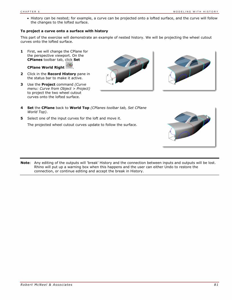
C H A P T E R 6 M O D E L I N G W I T H H I S T O R Y
Robert McNeel & Associates 81
History can be nested; for example, a curve can be projected onto a lofted surface, and the curve will follow the changes to the lofted surface.
To project a curve onto a surface with history
This part of the exercise will demonstrate an example of nested history. We will be projecting the wheel cutout curves onto the lofted surface.
1 First, we will change the CPlane for the perspective viewport. On the CPlanes toolbar tab, click Set
CPlane World Right .
2 Click in the Record History pane in the status bar to make it active.
3 Use the Project command (Curve menu: Curve from Object > Project) to project the two wheel cutout
curves onto the lofted surface.
4 Set the CPlane back to World Top (CPlanes toolbar tab, Set CPlane World Top).
5 Select one of the input curves for the loft and move it.
The projected wheel cutout curves update to follow the surface.
Note: Any editing of the outputs will 'break' History and the connection between inputs and outputs will be lost.
Rhino will put up a warning box when this happens and the user can either Undo to restore the
connection, or continue editing and accept the break in History.

C H A P T E R 6 M O D E L I N G W I T H H I S T O R Y
Robert McNeel & Associates 82
History enabled commands
Transforms Surfacing Solid Curve from object Annotation Point
Array
ArrayCrv
ArrayCrvOnSrf
ArrayPolar
ArraySrf
Bend (Copy option)
Copy
Orient (Copy option)
OrientCrvToEdge (Copy option)
OrientOnCrv (Copy option)
OrientOnSrf (Copy option)
Rotate (Copy option)
Scale (Copy option)
Mirror (Copy option)
Flow
FlowAlongSrf
ProjectToCPlane
RemapCPlane (Copy option)
Rotate (Copy option)
Rotate3D (Copy option)
Scale (Copy option)
Scale1D (Copy option)
Scale2D (Copy option)
ScaleByPlane (Copy option)
ScaleNU (Copy option)
SetPt
Shear
Stretch
Symmetry
Taper (Copy option)
Twist
EdgeSrf
ExtrudeCrv
ExtrudeCrvAlongCrv
ExtrudeCrvTapered
ExtrudeCrvToPoint
ExtrudeSrfToPoint
ExtrudeSrfAlongCrv
ExtrudeSrfTapered
Loft
NetworkSrf
OffsetSrf
Patch
PlanarSrf
RailRevolve
Revolve (Copy option)
Ribbon
Sweep1
Sweep2
TweenSurfaces
Pipe
Slab
ExtrudeSrf
ArcBlend
Blend
Crv2View
CSec
CrvThroughPolyline
CrvThroughPt
Helix (AroundCurve option)
Intersect
Offset
Project
Pull
Spiral (AroundCurve option)
TweenCurves
Dim
DimAligned
DimAngle
DimArea
DimCurveLength
DimDiameter
DimOrdinate
DimRadius
DimRotated
Hatch
Divide
History-related commands
History
HistoryPurge
SelObjectsWithHistory
SelChildren
SelParents
History toolbar
History Options
Inputs to a History-enabled command are called Parents in Rhino and the outputs are called Children.
Right-click the Record History pane to change the following options:
Always Record History
This option changes the default behavior so any eligible command will always record history. Use this option with caution. In addition to unnecessarily increasing the file size, it can lead to unexpected behavior. To clear history on particular objects or on all objects, use the HistoryPurge command.

C H A P T E R 6 M O D E L I N G W I T H H I S T O R Y
Robert McNeel & Associates 83
Update Children
Causes child objects to update each time the parent object changes. This increases the time it takes to update complex objects. For very complex edits on the parent objects, turn off updating, make the changes, and then
turn Update Children on so that the update happens only once.
Lock Children
This option sets child objects to a locked state. Since directly editing the child objects breaks the connection to the parent objects, locking the child objects prevents accidental editing. In addition, selecting child objects can be cumbersome if they are in the same location as the parent objects. Locked child objects still update when
the parent objects are edited.
History Break Warning
This option displays a warning if an operation breaks the connection of a child object to its parent objects. The Undo command will restore history.
Use the History command to control history recording, updating, locking, and warnings.
To change history options
1 Click on a curve to get the multi-select box.
If you edit the surface in any way, History for the object will break and Rhino will warn you about this.
2 Select the surface and drag it. Rhino will warn you that dragging broke
history. Click OK.
Make sure to Undo after getting a “broken History” warning to restore the connection between inputs and output.
3 Right-click in the Record History pane and check Lock Children.
This will make it impossible to edit a child in any way that will break history, but you can select it to change its object properties or layer,
etc.


Rober t McNeel & Assoc ia tes 85
7 Advanced surfacing techniques There are an infinite number of complex and tricky surfacing problems. In this chapter, we will look at several 'tricks' that help in getting certain types of surfaces built cleanly. The goal, apart from showing you a few specific techniques used in these examples, is to suggest ways in which the Rhino tools can be combined creatively to help solve surfacing problems.
In this chapter, you will learn to make soft domed button shapes, creased surfaces, and how to use curve-fairing techniques.
Dome-shaped buttons
The surfacing goal in this exercise is to create a dome on a shape like a cell
phone button where the top must conform to the general contour of the surrounding surface but maintain its own shape as well. There are a number of ways to approach this; we will look at three methods.
Exercise 20—Soft domed buttons
1 Open the model Button Domes.3dm.
The key to this exercise is defining a custom construction plane that represents the closest plane through the area of the surface that you want to match. Once you get the construction plane established, there is a variety of approaches available for building the surface.
There are several ways to define a construction plane. In this exercise, we will discuss four methods:
construction plane through three points, construction plane perpendicular to a curve, construction plane tangent to a surface, and fitting a plane to an object.
2 Use OneLayerOn to turn on the Surfaces to Match layer to see the surface that determines the cut of the
button.
To create a custom construction plane using three points method
1 Start the CPlane command with the
3Point option (View menu: Set CPlane > 3 Points).
2 In the Perspective viewport, using the Near object snap, pick three points on the edge of the trimmed hole.
The construction plane now goes through the three points. Notice the construction plane origin is at the
first point.
3 Rotate the Perspective viewport to see the grid aligned with the trimmed hole.

C H A P T E R 7 A D V A N C E D S U R F A C I N G T E C H N I Q U E S
Robert McNeel & Associates 86
To create a custom construction plane perpendicular to a curve
With a line normal to a surface and a construction plane perpendicular to that normal line, you can define a tangent construction plane at any given point on the surface
1 Start the CPlane command with the Previous option (Viewport title right-click menu: Set CPlane > Undo CPlane Change).
2 Use the Line command with the Normal option (Curve menu: Line > Normal to Surface) to draw a line
normal to the underlying surface at a point near the center of the trimmed hole.
Set the command-line option for IgnoreTrims=Yes so that the line can be drawn from a point inside the
trimmed hole in the surface.
3 Start the CPlane command with the Curve option (View menu: Set CPlane > Perpendicular to Curve).
4 Pick the normal.
5 Use the End object snap and pick the end of the normal where it intersects
the surface.
The construction plane is set perpendicular to the normal line.
To create a custom construction plane to a surface
This function sets the construction plane to match a surface. The placement is constrained so that the construction
plane is tangent to the surface at any given point on the surface. This works like the previous method without the need to make the normal line.
1 Start the CPlane command with the Previous option (Viewport title right-
click menu: Set CPlane > Undo CPlane Change).
2 Delete the Normal line.
3 Start the CPlane command (View menu: Set CPlane > Origin) with the Surface option.
4 Pick the surface.
5 For the CPlane origin, change the
IgnoreTrims option to Yes, then pick a point near the center of the hole.
6 For the X axis direction, pick a point in the direction of the long dimension
of the trim curve.
The construction plane is set tangent to the surface at the origin.

C H A P T E R 7 A D V A N C E D S U R F A C I N G T E C H N I Q U E S
Robert McNeel & Associates 87
To create a construction plane fit through points
Using the PlaneThroughPt command to create a surface through a sample of extracted point objects will generate a plane that best fits the points. The CPlane command with the Object option places a construction
plane with its origin on the center of the plane. This is a good choice in the case of the button in this file. There are several curves from which the points can be extracted—the edge of the button itself, or from the trimmed hole in the surrounding surface.
1 Start the CPlane command with the Previous option (Viewport title right-click menu: Set CPlane > Undo CPlane Change).
2 Turn on the Surfaces and the Curves layer. Make the Curves layer the
current layer.
3 Start the DupEdge command (Curve menu > Curve from objects > Duplicate edge) to duplicate the top edge of the button surface, press Enter.
4 Copy the duplicated curve vertically twice.
The vertical position of these curves will determine the shape of the
button.
5 Use the Divide command (Curve menu: Point Object>Divide curve by>Number of segments) to mark off the top copied curve with 50 points. Set the command line options to Split=No and GroupOutput=Yes
6 Use SelLast to select the points just created.
7 Use the PlaneThroughPt command (Surface menu: Plane > Through
Points) with the selected points.
8 Press the Delete key to delete the point objects that are still selected.
A rectangular plane is fit through the selected points.
9 Use the CPlane command with the Object option (View menu: Set CPlane > To Object) to align the construction plane with the plane.

C H A P T E R 7 A D V A N C E D S U R F A C I N G T E C H N I Q U E S
Robert McNeel & Associates 88
10 From the View menu, select Set CPlane, click Named CPlanes, then click the SaveAs icon to save and name the custom construction plane
Button Top.
This will allow you to restore this custom construction plane at any time.
11 Delete the surface you used to create the Button Top construction plane.
To loft the button
1 Set the Surfaces layer as the current layer.
2 Use Loft to make the button.
3 Select the top edge of the surface and the two copied curves.
4 After selecting the curves, click Point on the command line.
5 For the Loft endpoint, make sure the view that has the custom construction plane is the current view, then type 0 (zero) and press Enter.
The loft will end at a point in the middle of the plane, which is the origin of the construction plane.
6 In the Loft Options dialog, under Style, choose Loose, press OK.
With the Loose option, the control points of the input curves
become the control points of the resulting surface, as opposed to the Normal option, in which the lofted surface is interpolated through the curves.

C H A P T E R 7 A D V A N C E D S U R F A C I N G T E C H N I Q U E S
Robert McNeel & Associates 89
7 Turn on control points on the lofted surface.
8 Select the next ring of points out from the
center.
Select one point and use SelV or SelU to select the whole ring of points.
9 Use the SetPt command (Transform menu: Set XYZ Coordinates) to set the points to the same Z-elevation as the point in the center. Set the radio button in the dialog to Align to CPlane.
Remember, this elevation is relative to the current construction plane.
Note: You can use History when creating the loft, in which case the SetPt operation should be applied to the
topmost curve in the loft, not to the loft surface control points.
To use a patch surface to make the button
1 Use the DupEdge command to duplicate the top edge of the surface.
2 Move the duplicated curve in the World Z-direction a small amount.
3 Use Divide to mark off this curve with 50 points as before.
4 Use the PlaneThroughPt command with the selected points, and then
delete the points like the previous exercise.
5 Use the CPlane command with the Object option to set the construction plane to the planar surface.
6 Make a circle or ellipse centered on the origin of the custom construction plane.
7 Use the Patch command, selecting the top edge of the button and the ellipse or circle.
The surface is tangent to the edge and concave on the top.
The size and vertical position of the circle/ellipse will affect the shape of
the surface.
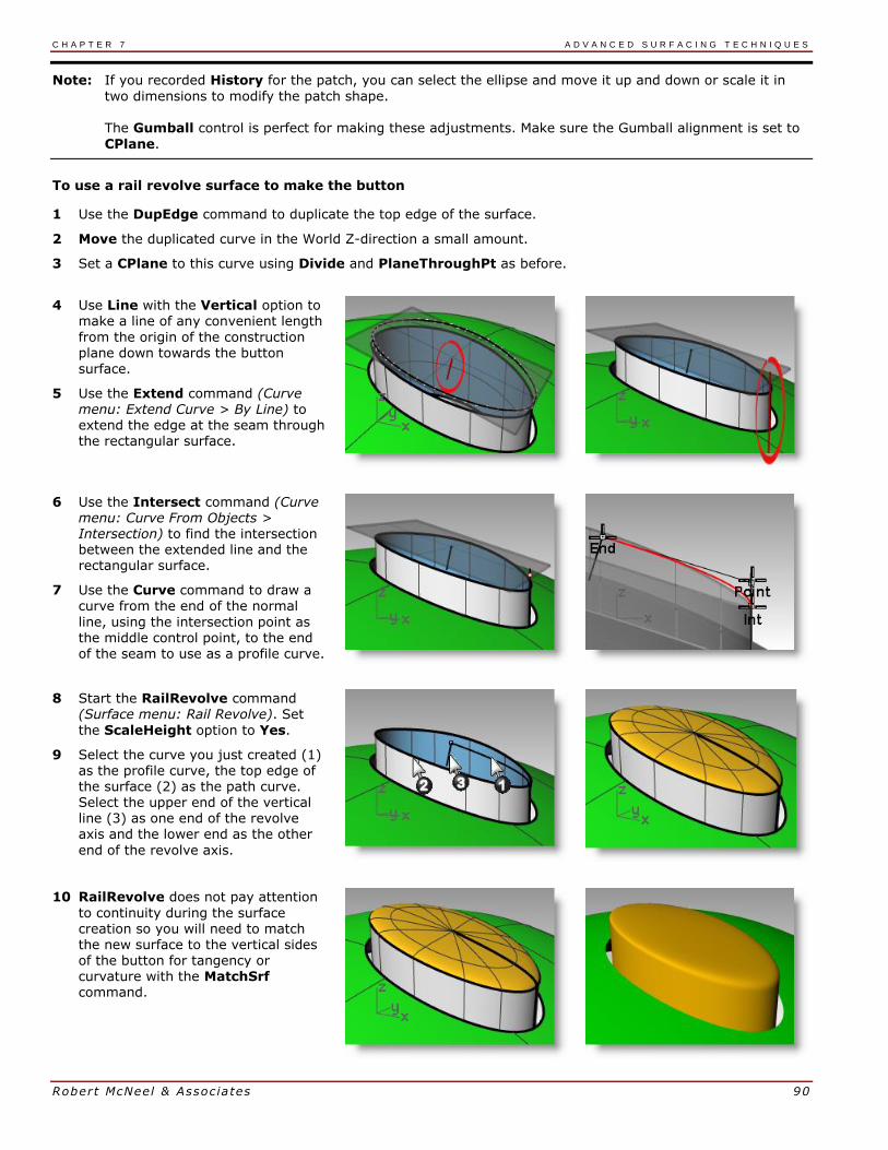
C H A P T E R 7 A D V A N C E D S U R F A C I N G T E C H N I Q U E S
Robert McNeel & Associates 90
Note: If you recorded History for the patch, you can select the ellipse and move it up and down or scale it in
two dimensions to modify the patch shape.
The Gumball control is perfect for making these adjustments. Make sure the Gumball alignment is set to
CPlane.
To use a rail revolve surface to make the button
1 Use the DupEdge command to duplicate the top edge of the surface.
2 Move the duplicated curve in the World Z-direction a small amount.
3 Set a CPlane to this curve using Divide and PlaneThroughPt as before.
4 Use Line with the Vertical option to make a line of any convenient length
from the origin of the construction plane down towards the button
surface.
5 Use the Extend command (Curve menu: Extend Curve > By Line) to extend the edge at the seam through the rectangular surface.
6 Use the Intersect command (Curve menu: Curve From Objects > Intersection) to find the intersection between the extended line and the rectangular surface.
7 Use the Curve command to draw a
curve from the end of the normal
line, using the intersection point as the middle control point, to the end of the seam to use as a profile curve.
8 Start the RailRevolve command (Surface menu: Rail Revolve). Set
the ScaleHeight option to Yes.
9 Select the curve you just created (1) as the profile curve, the top edge of the surface (2) as the path curve. Select the upper end of the vertical line (3) as one end of the revolve axis and the lower end as the other
end of the revolve axis.
10 RailRevolve does not pay attention
to continuity during the surface creation so you will need to match the new surface to the vertical sides of the button for tangency or curvature with the MatchSrf command.

C H A P T E R 7 A D V A N C E D S U R F A C I N G T E C H N I Q U E S
Robert McNeel & Associates 91
Creased surfaces
Often a surface needs to be built with a crease that may start at
a particular angle and change to another angle or diminish to zero. The crease in the car body in the image is an example of this. The following exercise covers two possible situations.
Exercise 21—Surfaces with a crease
The key to the following exercise is to get two surfaces that match with different continuity at each end. At one
end, we will match the surface with a 10-degree angle, and at the other end, we will match the surface with
tangency continuity. To accomplish this we will create a dummy surface at the correct angles and use this to match the lower edge of the upper surface. When the dummy surface is deleted or hidden, the crease appears between the two surfaces we want to keep.
1 Open the model Crease 01.3dm.
2 Turn on the Curve and Loft layers.
3 Make the Loft layer current.
4 Use the Loft command to make a surface from the three curves.
The Loft command remembers the settings across sessions. Make sure the Loft style is set to Normal and Do not simplify.
5 We are going to make a surface that
includes all the curves but has a crease along the middle curve.
Use the middle curve to Split the resulting surface into two pieces.
6 Use the ShrinkTrimmedSrf command (Surface menu: Surface Edit Tools > Shrink Trimmed Surface) on both
surfaces.
With a surface that results from a split at an isocurve, shrinking it will allow the edge to be an untrimmed edge because the trim corresponds to the natural
untrimmed surface edge.
By trimming with a curve used in the
loft, the curve is in effect an isocurve.
You can also use the Isocurve option in the Split command when the object to be split is a single surface.
7 Hide the lower surface and turn off the Curve layer.
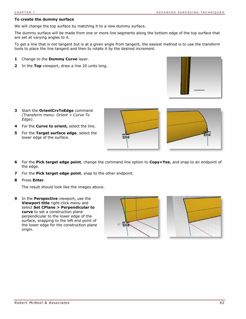
C H A P T E R 7 A D V A N C E D S U R F A C I N G T E C H N I Q U E S
Robert McNeel & Associates 92
To create the dummy surface
We will change the top surface by matching it to a new dummy surface.
The dummy surface will be made from one or more line segments along the bottom edge of the top surface that
are set at varying angles to it.
To get a line that is not tangent but is at a given angle from tangent, the easiest method is to use the transform tools to place the line tangent and then to rotate it by the desired increment.
1 Change to the Dummy Curve layer.
2 In the Top viewport, draw a line 20 units long.
3 Start the OrientCrvToEdge command (Transform menu: Orient > Curve To Edge).
4 For the Curve to orient, select the line.
5 For the Target surface edge, select the lower edge of the surface.
6 For the Pick target edge point, change the command line option to Copy=Yes, and snap to an endpoint of the edge.
7 For the Pick target edge point, snap to the other endpoint.
8 Press Enter.
The result should look like the images above.
9 In the Perspective viewport, use the Viewport title right-click menu and select Set CPlane > Perpendicular to
curve to set a construction plane perpendicular to the lower edge of the surface, snapping to the left end point of the lower edge for the construction plane origin.
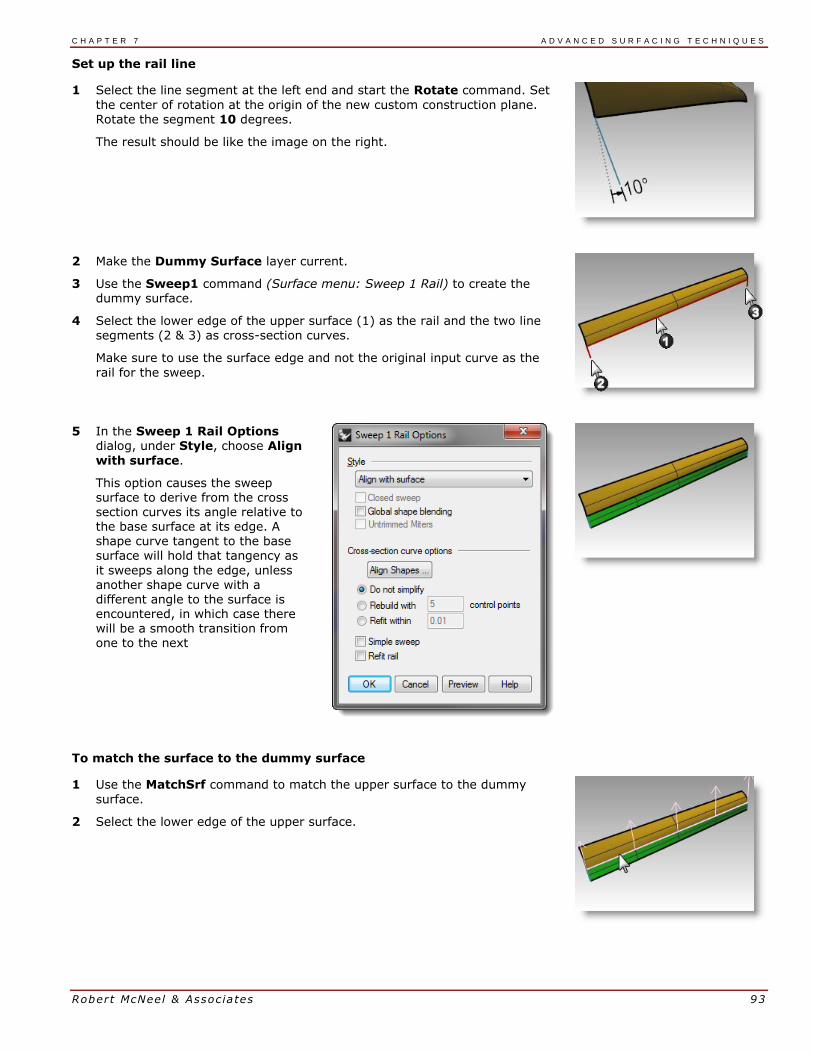
C H A P T E R 7 A D V A N C E D S U R F A C I N G T E C H N I Q U E S
Robert McNeel & Associates 93
Set up the rail line
1 Select the line segment at the left end and start the Rotate command. Set
the center of rotation at the origin of the new custom construction plane.
Rotate the segment 10 degrees.
The result should be like the image on the right.
2 Make the Dummy Surface layer current.
3 Use the Sweep1 command (Surface menu: Sweep 1 Rail) to create the dummy surface.
4 Select the lower edge of the upper surface (1) as the rail and the two line
segments (2 & 3) as cross-section curves.
Make sure to use the surface edge and not the original input curve as the
rail for the sweep.
5 In the Sweep 1 Rail Options dialog, under Style, choose Align
with surface.
This option causes the sweep surface to derive from the cross section curves its angle relative to the base surface at its edge. A shape curve tangent to the base
surface will hold that tangency as
it sweeps along the edge, unless another shape curve with a different angle to the surface is encountered, in which case there will be a smooth transition from one to the next
To match the surface to the dummy surface
1 Use the MatchSrf command to match the upper surface to the dummy
surface.
2 Select the lower edge of the upper surface.
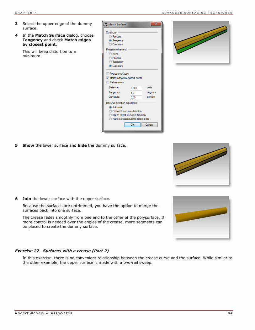
C H A P T E R 7 A D V A N C E D S U R F A C I N G T E C H N I Q U E S
Robert McNeel & Associates 94
3 Select the upper edge of the dummy surface.
4 In the Match Surface dialog, choose Tangency and check Match edges by closest point.
This will keep distortion to a minimum.
5 Show the lower surface and hide the dummy surface.
6 Join the lower surface with the upper surface.
Because the surfaces are untrimmed, you have the option to merge the surfaces back into one surface.
The crease fades smoothly from one end to the other of the polysurface. If more control is needed over the angles of the crease, more segments can be placed to create the dummy surface.
Exercise 22—Surfaces with a crease (Part 2)
In this exercise, there is no convenient relationship between the crease curve and the surface. While similar to the other example, the upper surface is made with a two-rail sweep.

C H A P T E R 7 A D V A N C E D S U R F A C I N G T E C H N I Q U E S
Robert McNeel & Associates 95
To create a crease with trimmed surfaces
1 Open the model Crease 02.3dm.
2 Use the Line command (Curve menu: Line > Single Line) to draw a single line anywhere in the top or perspective viewport.
We will use this line to make a dummy surface.
3 Use the OrientCrvToEdge command (Transform menu: Orient > Curve to Edge) to copy the curve for the dummy surface to the upper edge of the lower surface.
4 Place a line at each end of the edge and somewhere in the middle of the
edge.
5 Move each line segment by moving its upper end to the lower end of the same segment.
6 Use the CPlane command (View menu:
Set CPlane > Perpendicular to Curve) to set the construction plane to align with the line at the left of the surface.
7 Use the Rotate command (Transform menu: Rotate) to rotate the line 15 degrees as shown in the illustration on the right.

C H A P T E R 7 A D V A N C E D S U R F A C I N G T E C H N I Q U E S
Robert McNeel & Associates 96
8 Repeat these steps for the line in the middle of the surface.
To make the dummy surface
1 Use the Sweep1 command to create the dummy surface.
2 Select the upper edge of the lower surface as the rail and the three line segments as cross-section curves. Use the Align with surface style for
the sweep.
3 Hide the original surface.
4 Use the Sweep2 command to make the upper surface.
Choose the upper edge of the dummy surface as a rail (1) and the long curve at the top as the other rail (2).
Choose the curves at both ends as the cross-section curves (3) and (4).

C H A P T E R 7 A D V A N C E D S U R F A C I N G T E C H N I Q U E S
Robert McNeel & Associates 97
5 In the Sweep 2 Rails Options dialog, for the Rail continuity of
edge A, choose Tangency.
6 Delete the dummy surface.
7 Use Show or Show Selected (Edit menu>Visibility>Show selected) to show the original lower surface.
8 Join the lower surface with the
upper surface.
Curve fairing to control surface quality
Curves in Rhino can come from many sources, they can be:
Created in Rhino directly
Imported from digitized data
Imported from another application
Section curves generated from a mesh
It is important to understand that many of these curves need to be optimized for quality.
Fairing is a technique used to simplify curves while improving their curvature graphs and keeping their shape within tolerance. It is especially important to fair curves that are generated from digitized data, intersections,
extracted isocurves, or curves from two views.
Generally, curves that are single-span curves work better for this process. A single span curve is a curve that has one more control point than the degree. For examples a degree 3 curve with 4 control points, a degree 5 curve with 6 control points, or a degree 7 curve with 8 control points.
To analyze a lofted surface with curvature analysis
1 Open the model Fair Curves.3dm.
2 Select the curves and use the Loft command (Surface menu: Loft) with Style set to Normal and Cross-
section curve options set to Do not simplify to make a surface.
The surface is very complex. It has
many more isocurves than are needed to define the shape, because the knot structures of the curves are very different.
The surface also has compound curvature.

C H A P T E R 7 A D V A N C E D S U R F A C I N G T E C H N I Q U E S
Robert McNeel & Associates 98
3 Select the lofted surface and start the CurvatureAnalysis command (Analyze menu > Surface>Curvature analysis).
This creates a so-called “False color” display using the same type of analysis meshes as the Zebra command.
The amount of curvature is mapped to a range of colors allowing you to analyze for areas of abruptly changing curvature or flat spots.
Choose Mean from the Style drop down.
This style is useful for showing discontinuities in the curvature—flat spots and dents. The mean is between the two curvature circle values at each point, mapped to a color
value.
4 Push the AutoRange button.
5 Click the Adjust mesh button and adjust the Minimum initial grid quads to have at least 5000 minimum grid quads to ensure a smooth display of the color range.
Note the streaky and inconsistent colors on the surface. This indicates
abrupt changes in the surface.
6 Undo the loft.

C H A P T E R 7 A D V A N C E D S U R F A C I N G T E C H N I Q U E S
Robert McNeel & Associates 99
To rebuild the curves
1 Change to the Tangency Direction
layer.
2 Use the Line command (Curve menu: Line>Single Line,) with the Extension option, to make a line that maintains the tangency direction of an original curve from each end point and coming back towards the curve,
any length.
Make the lines long enough to cross one another.
3 Change to Rebuilt Curves layer, and Lock the Tangency Direction
layer
4 Use the Rebuild command (Edit menu: Rebuild) to rebuild the curve.
Although there is a Rebuild option in the Loft command, rebuilding the curves before lofting them gives you control over the degree of the curves as well as the number of control points.
5 In the Rebuild Curve dialog, change the Degree to 5 and the Point Count to 6 points. Uncheck Delete input, check Create new curve on
Current layer. Click the Preview button. Note how much the curves deviate from the originals.
This makes the curves into single-span curves. Single-span curves are Bézier curves. A single-span curve is a curve that has degree +1 control points. While this is not necessary to get high quality surfaces, it produces predictable results.
6 Lock the Original Curves layer. We need to see these curves but we do
not want to be able to select them.
7 Select one of the rebuilt curves, and turn on the Control points and Curvature graph.
8 Fair the curve by adjusting points until it matches the original curve
closely enough.
Start by moving the second point from each end of the rebuilt curve onto the tangent line. Use the Near object snap to drag along the tangent line.
9 Check the curvature graph to make sure the curve has smooth
transitions.
The curves are fair when the points are adjusted so the rebuilt curves match the original locked curves closely, with good graphs.
10 Fair the other curves the same way.

C H A P T E R 7 A D V A N C E D S U R F A C I N G T E C H N I Q U E S
Robert McNeel & Associates 100
Here are some things to keep in mind when adjusting the curves:
If you want to keep the curve tangent direction consistent with the original curves, make sure the second point from each curve stays on the green tangent direction line- only move these points with the Near
object snap pulling the point onto the line.
The DragMode command, set to ControlPolygon will constrain point dragging to the curve control polygon- you can use this tool to keep the tangent directions constant.
Where possible, when fairing a set of curves to be used as input to a single lofted surface, try to keep the control point arrangement on each curve similar to the neighboring curves. This will help keep the surface nicely aligned.
When control point adjustment becomes difficult due to the small movements needed, try using the Nudge
keys to nudge the points by small amounts. See Help for more information about Nudge.
You can also use the Gumball to move points. When fine-tuning with very small point movements needed, you can set GumballDragStrength to something less than 100% to allow larger mouse movements to make small changes in the point locations.
To use PointDeviation to visualize the deviation while you edit the curves
1 Make a Points layer and make it current.
2 Select all of the original curves and start the Divide command (Curve menu: Point Object>Divide Curve by>Number of Points). Set the Number of segments to 32 and GroupOutput=Yes.
3 Deselect all objects, and select the grouped points.
4 Start the PointDeviation command (Analyze menu: Surface>Point Set Deviation), and at the Select curves, surfaces, and polysurfs to test
prompt, select the, roughly faired, rebuilt curves.
5 When the Point/Surface Deviation dialog pops up, set the numbers as follows:
Good point = 0.1 Bad point = 0.5 Ignore = 1.0
The display shows the deviation between the points displayed on the original curves and the closest locations to these on the rebuilt curves.
6 Lock the Points and the Original Curves layers.
7 Continue to modify the rebuilt curves with the goal being that all points will turn blue, as good points.
Note: If you close the dialog, you lose the display and you need to
start over with PointDeviation.

C H A P T E R 7 A D V A N C E D S U R F A C I N G T E C H N I Q U E S
Robert McNeel & Associates 101
To make a surface with fair curves
1 Loft the new curves.
The shape and quality of the surface has very few isocurves but it is very close to the shape of the first surface.
2 Analyze the surface with CurvatureAnalysis.
Note the smooth transitions in the false color display, indicating smooth curvature transitions in the surface.


Rober t McNeel & Assoc ia tes 103
8 Use background bitmaps This exercise describes the steps in creating a case for a small, hand held product, using bitmaps as templates. In this exercise, we will focus on making curves from bitmap images and using fairing techniques on the curves before making the surfaces.
We will begin by taking scanned sketches and placing them in three different viewports. The three hand-drawn images need to be placed in their respective viewports and scaled appropriately so that they match each other.
You can align images more easily if they have been aligned and cropped so that they share the same length in pixels. It helps to darken and slightly reduce the contrast of images that have a lot of bright white in them. This
allows a greater range of colors to be seen against them when tracing them in Rhino.
Exercise 23—Handset
1 Open the model Handset.3dm.
2 From the Tools menu, click Toolbar Layout.
3 In the Rhino Options dialog, on the Toolbars page, check Background Bitmap to open the toolbar, and
then close the dialog.
Use the toolbar buttons for the next part of the exercise.
The toolbar can also be accessed by flying out the Background Bitmap toolbar from the Viewport Layout tab across the top.
4 It will make it easier in this exercise if you Split the Front Viewport horizontally and make the lower viewport the Bottom view. You can re-align the views like the illustration below.
5 In Rhino Options, on the View page, in the Viewport properties section, check Linked viewports.
This allows the viewports to stay aligned with each other when zooming and panning.
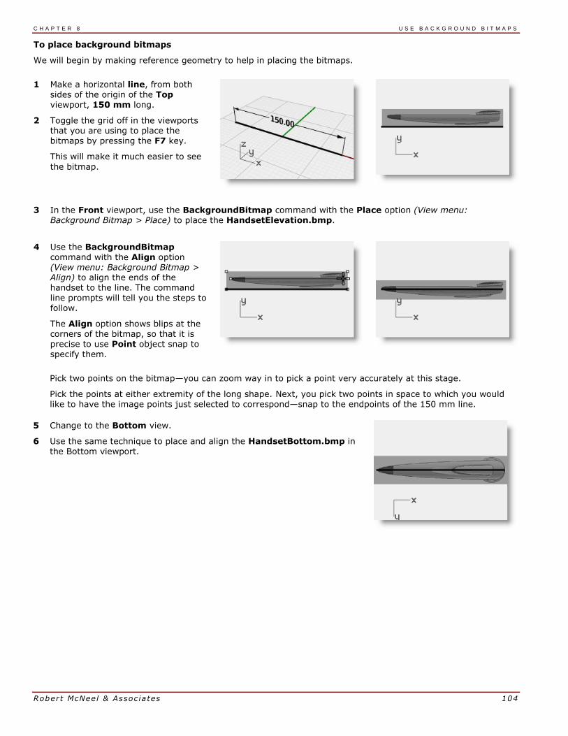
C H A P T E R 8 U S E B A C K G R O U N D B I T M A P S
Robert McNeel & Associates 104
To place background bitmaps
We will begin by making reference geometry to help in placing the bitmaps.
1 Make a horizontal line, from both sides of the origin of the Top viewport, 150 mm long.
2 Toggle the grid off in the viewports that you are using to place the bitmaps by pressing the F7 key.
This will make it much easier to see
the bitmap.
3 In the Front viewport, use the BackgroundBitmap command with the Place option (View menu: Background Bitmap > Place) to place the HandsetElevation.bmp.
4 Use the BackgroundBitmap command with the Align option (View menu: Background Bitmap > Align) to align the ends of the handset to the line. The command
line prompts will tell you the steps to follow.
The Align option shows blips at the corners of the bitmap, so that it is precise to use Point object snap to specify them.
Pick two points on the bitmap—you can zoom way in to pick a point very accurately at this stage.
Pick the points at either extremity of the long shape. Next, you pick two points in space to which you would like to have the image points just selected to correspond—snap to the endpoints of the 150 mm line.
5 Change to the Bottom view.
6 Use the same technique to place and align the HandsetBottom.bmp in the Bottom viewport.

C H A P T E R 8 U S E B A C K G R O U N D B I T M A P S
Robert McNeel & Associates 105
7 Repeat these steps for the Top viewport.
To build the case
The most useful tool for tracing freeform curves is a control point curve.
Place the fewest number of points that will accurately describe the curve. Do not fall into the trap of trying to be 100% accurate with every point placement. With some experience you will be able to place about the right number of points in about the right places and then point edit the curve into its final shape.
In this example, the 2-D curves can all be drawn quite accurately with a degree-3 curve using five or at most six control points.
Remember to pay attention to the placement of the second points of the curves to maintain tangency across the
pointed end of the object.
1 In the Front viewport, trace two curves to define the form of the case.
The front view curves describing the top and bottom edges of the case
should extend on the right past the
form in the background image.
2 In the Bottom viewport, trace one curve to define the form of the case.
Since the bottom view of the object is symmetrical, you can make one curve. Extend the curve past the background image approximately the same distance as you did with the curves in the front viewport.

C H A P T E R 8 U S E B A C K G R O U N D B I T M A P S
Robert McNeel & Associates 106
3 Draw the curve in the Front viewport that defines the parting line
separating the top and bottom halves
of the case.
This curve is the front view of the plan view’s edge curves. It should be extended to the right the same distance as the other edge curves.
4 Trim both bottom view and front
view form curves with a single cutting plane or use the SetPt command to set the points at the same plane.
5 In the Perspective viewport, select
the parting line curve and the outline curve that you created in the Bottom
viewport.
6 Use the Crv2View command (Curve menu: Curve From 2 Views) to create a curve based on the selected curves.
A 3-D curve is created.
7 Hide or Lock the two original curves.
Now there are three curves.
8 Turn on the control points for the curves.
Notice the number of control points
and the spacing. This is an example of curves that need to be faired before you can create a good surface from them.
9 Fair the curves, using the same technique as in the previous exercise.
10 Mirror the 3-D curve for the other side.
The macros ! Mirror 0 1,0,0 and ! Mirror 0 0,1,0 are very useful for
accomplishing this quickly if they are assigned to a command alias
and if the geometry is symmetrical about the x- or y-axis.

C H A P T E R 8 U S E B A C K G R O U N D B I T M A P S
Robert McNeel & Associates 107
11 Loft the faired curves with the Closed loft option checked.
Notice the quality of the surface and how few isocurves there are.
A closed loft will have a seam.
To build the case (alternate technique 1)
1 Undo until your back to step 7 of the previous part of the exercise.
2 Mirror the 3-D curve for the
other side.
3 Loft the curves, using the Rebuild option to 18 points.
The isocurves all true up and everything looks clean, but if you look at the tip, it falls away from the input curves.
The Rebuild option does not sample more in areas of high curvature but just divides the curves up evenly.
To fair the surface
1 Hide the background bitmaps and set the viewport to wireframe.
2 Turn on surface points.
3 In the top or bottom view, move points on one side of the surface in the y-direction to get the surface to match.
A few points moved should do it.
Now, how do we get the other side exactly the same?
4 Undo all the moves and instead of moving the points, select opposite
pairs of points and Scale1D in Y to move them symmetrically.
The base of the scale should be a middle point, use Ortho to keep the scale axis true to Y.

C H A P T E R 8 U S E B A C K G R O U N D B I T M A P S
Robert McNeel & Associates 108
5 Show the Organic toolbar and use the Expand Y and Compress Y nudge controls to do the same thing in small increments.
These buttons are macros of Scale1D using the origin as the scale origin.
6 Use similar techniques for adjusting points in the elevation view. Since the points in this view are not symmetrical in the z-axis, do one side at a time, moving rather than scaling the points.
Nudge keys or the Move in Z nudge controls in the Organic toolbar also
work.
To build the case using the CSec command (alternate technique 2)
The CSec command creates cross-section curves through profile curves.
1 Undo back to the four input curves.
2 Start the CSec command (Curve menu > Cross section profiles).
3 Select the curves in order as if lofting them, make sure the Closed option is Yes, press Enter when done.
4 For the Start cross-section line, in
Front viewport, pick a point on either side of the 4 curves.
5 For the End of cross-section line, use Ortho, and pick a point on the other side of the 4 curves.
6 Continue this process until you have 6-10 cross-section curves, evenly
spaced along the four curves
Make sure to add one section snapping to the endpoints at the open end of the set of curves.

C H A P T E R 8 U S E B A C K G R O U N D B I T M A P S
Robert McNeel & Associates 109
7 Window the section curves and the original long curves.
8 Start the NetworkSrf command (Surface menu > Curve Network) to
make the surface.


Rober t McNeel & Assoc ia tes 111
9 An approach to modeling A common question that users have when modeling, is “Where do I start?” In this section, we will discuss various approaches to the modeling process.
There are two things to consider before your begin modeling: if reflections, fluid flow, air flow, or the ability to edit using control points are important in the finished model, you will want to begin your models with geometry that consists of cubic (degree 3) or quintic (degree 5) curves. If these are not important, you can use a combination of linear (degree 1), quadratic (degree 2), cubic or quintic curves.
Start with simple shapes, the details can be added later. Begin by creating layers for the different parts. This will
help separate the parts for visualization, and help with matching the parts as you go.
We will review different products to try to determine which kind of surfaces are most important and some approaches to modeling the product.
Exercise 24—Cutout
This exercise shows an approach to making a cutout surface that blends
smoothly and seamlessly into an existing curved surface. The new surface has an arbitrary relationship to the existing surface so the general strategy can be used in other cases.
For this exercise, we have created additional models for each stage of the exercise. The models are for reference and include notes to explain the procedure for the steps in that stage of the exercise. There will be a note at each stage to indicate which model to open if needed.
1 Open the model Scoop.3dm.
2 Make the Cut-out Curves layer current, turn on the Original
Surface layer, and turn off the
Completed Scoop layer.
3 In the Top viewport, select the curves.
4 Start the Project command (Curve menu: Curve From Objects > Project).
5 Select the surface and press Enter.
The curves will be projected onto the surface.
6 Start the ExtendCrvOnSrf command
(Curve menu: Extend Curve > Curve
on Surface).
7 For the Curve to extend, select the outer curve on the surface.
8 Select the surface.
The ends of the curve are extended
to the edge of the surface.
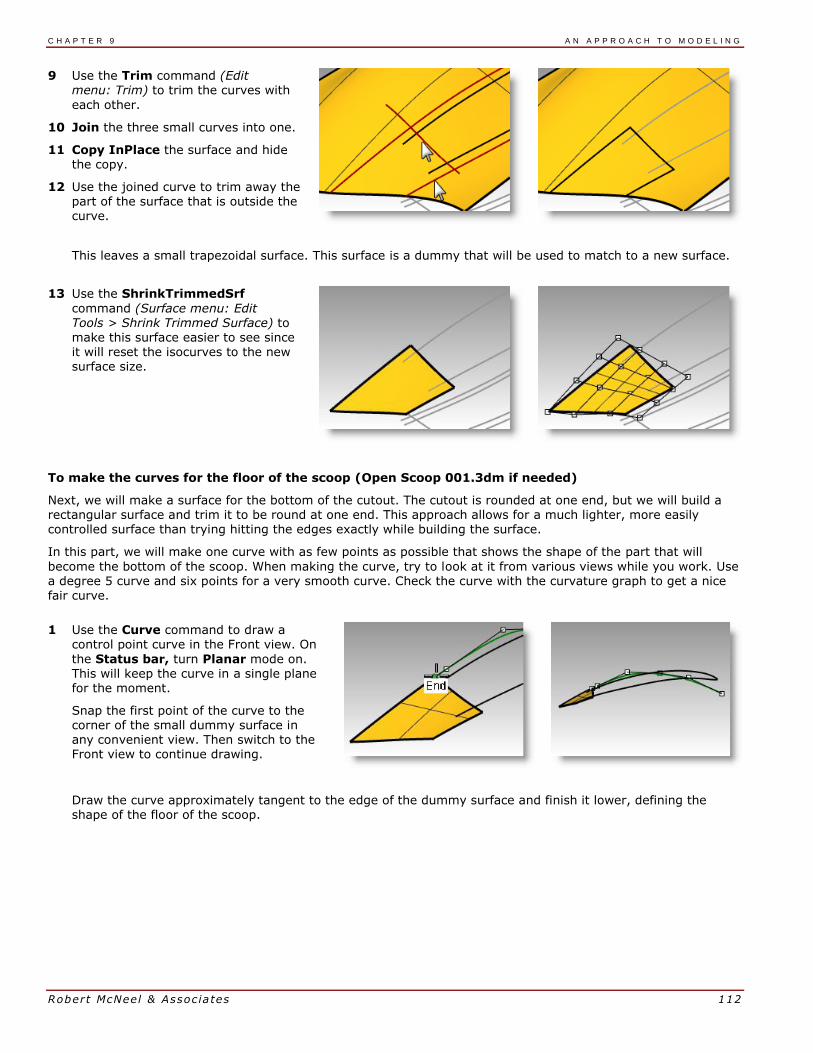
C H A P T E R 9 A N A P P R O A C H T O M O D E L I N G
Robert McNeel & Associates 112
9 Use the Trim command (Edit menu: Trim) to trim the curves with
each other.
10 Join the three small curves into one.
11 Copy InPlace the surface and hide the copy.
12 Use the joined curve to trim away the part of the surface that is outside the curve.
This leaves a small trapezoidal surface. This surface is a dummy that will be used to match to a new surface.
13 Use the ShrinkTrimmedSrf
command (Surface menu: Edit Tools > Shrink Trimmed Surface) to
make this surface easier to see since it will reset the isocurves to the new surface size.
To make the curves for the floor of the scoop (Open Scoop 001.3dm if needed)
Next, we will make a surface for the bottom of the cutout. The cutout is rounded at one end, but we will build a rectangular surface and trim it to be round at one end. This approach allows for a much lighter, more easily controlled surface than trying hitting the edges exactly while building the surface.
In this part, we will make one curve with as few points as possible that shows the shape of the part that will
become the bottom of the scoop. When making the curve, try to look at it from various views while you work. Use a degree 5 curve and six points for a very smooth curve. Check the curve with the curvature graph to get a nice fair curve.
1 Use the Curve command to draw a control point curve in the Front view. On
the Status bar, turn Planar mode on. This will keep the curve in a single plane for the moment.
Snap the first point of the curve to the corner of the small dummy surface in any convenient view. Then switch to the Front view to continue drawing.
Draw the curve approximately tangent to the edge of the dummy surface and finish it lower, defining the shape of the floor of the scoop.

C H A P T E R 9 A N A P P R O A C H T O M O D E L I N G
Robert McNeel & Associates 113
2 Adjust the curve with point editing to get the right shape in the Top view.
Make sure to move the points only in the y-direction (Ortho will help), so that the shape in the Front view will not be altered.
Make the curve approximate the outermost of the original curves and extend somewhat past the rounded end.
3 Use the Match command (Curve menu: Curve Edit Tools > Match) to match the curve with Curvature continuity to the edge of the dummy surface.
Edit the curve further if needed but be sure to use Match again if you have
moved any of the first three points in the curve.
4 Copy the curve to the other edge.
5 Adjust the curves by moving the control points until they look the way you want, and then Match the curve to the edge of the dummy surface.
If matching makes the curve distort too much add a knot and try again. Using
the EndBulge command and further point editing may be needed.
To create the floor surface of the scoop (Open Scoop 002.3dm if needed)
There are a few surfacing techniques that can be used to create the surface.
A 2-Rail Sweep would be one obvious choice, using the new curves as rails and the edge of the
dummy surface as the cross section. The advantage of this is that other cross-sections can be used to define the floor shape if desired.
Since the rails are G2 to the dummy
surface (Matched in the last sequence of steps), the surface will
be very close to G2 to the dummy surface when created.
The MatchSrf command could fix any discontinuity, if needed. This is a good way to go and you may wish to try it now.
2-Rail Sweep using the new curves as rails and the surface edge as the cross-section.
2-Rail Sweep using the new curves as rails and the surface edge as the cross-section with the simple sweep option checked.
Another approach is to make a lofted surface between the two curves. The surface will need adjustment to match to the dummy surface and will provide the opportunity to explore some options in the MatchSrf command so we will outline this method below.

C H A P T E R 9 A N A P P R O A C H T O M O D E L I N G
Robert McNeel & Associates 114
1 Use the Loft command (Surface menu: Loft) to create the surface
between the two curves.
Because the lofted surface is flat, there will be a slight gap at the edge of the dummy surface.
2 Use the MatchSrf command (Surface
menu: Surface Edit Tools > Match) to match the lofted surface to the edge of the dummy surface for curvature.
Use the Preview button to see how the match will look.
You may notice that the matched
surface pulls around quite drastically to be perpendicular to the target edge.
If so, change the Isocurve adjustment from Automatic to Preserve isocurve direction, and try the Preview again. The surface should
now match with much less distortion.
3 Use the Zebra command (Analyze menu: Surface > Zebra) to check the continuity of the two surfaces.
To make the sides of the cutout (Open Scoop 003.3dm if needed)
To make the sides of the cutout, we will extrude the projected outline with 10 degrees of draft and trim it with the lofted surface.
1 Select the outer projected curve.
2 Use the ExtrudeCrvTapered command (Surface menu: Extrude curve >Tapered) to extrude the outer projected curve. Change the DraftAngle to 10. Pull the surface until it fully intersects with the bottom
surface, but no more, and pick.
If you extrude the surface too far, you might get a polysurface instead
of a single surface.
If this happens try to extrude again, but do not pull so far.
If you cannot pull it far enough to penetrate the floor without making a polysurface, extrude it a short distance instead.

C H A P T E R 9 A N A P P R O A C H T O M O D E L I N G
Robert McNeel & Associates 115
3 Use the ExtendSrf command (Surface menu: Extend Surface) to extend it through the floor surface.
The extruded surface is a very dense surface.
4 Use the FitSrf command (Surface menu: Surface Edit Tools >Refit to Tolerance) to simplify the surface.
A Fitting tolerance of 0.001 with DeleteInput=Yes, ReTrim=Yes, UDegree=3, and VDegree=3 should work well.
To create the fillets
Now the surfaces are ready to be filleted.
1 Show the main surface and Hide the dummy surface.
2 Use the FilletSrf command (Surface menu: Fillet Surface) with a
Radius=5, Extend=No, and Trim=No to make the fillets between the bottom surface and the sides.
3 For the first surface to fillet, pick the bottom surface.
4 Pick the side surface near the same spot.
5 Repeat this for the side surface and the original surface.
The two fillets cross each other. We will trim them both back to their intersection points.
Where you pick matters.
Trimming the fillet surfaces (Open Scoop 004.3dm if needed)
Both of the fillet surfaces are tangent to the tapered side of the scoop. Where the fillets cross they are tangent to
each other.
If we trim the ends of the fillets to a plane, then the resulting trimmed edges will be tangent to each other. Trimming these surfaces will be helpful when creating the final surfaces that blend the fillets out between the
scoop and main surfaces.
To create the plane, first make circles with the AroundCurve option around one edge of the fillet surfaces, then make planar surfaces from the circles.
1 Select the fillets and use the Invert Hide button in the visibility toolbar
to isolate them.
2 Start the Circle command, and use the AroundCurve option. Set the Int object snap only.
The AroundCurve option forces the circle command to look for curves, including edge curves, to
draw the circle around.
3 Click on the upper edge of the lower surface and snap to the intersection point.

C H A P T E R 9 A N A P P R O A C H T O M O D E L I N G
Robert McNeel & Associates 116
4 Draw the circle out well past the width of the fillet surfaces.
5 Use the PlanarSrf command (Surface menu: Planar Curves) to create a circular surface at the intersection point.
6 Repeat these steps for the other intersection.
7 Trim the fillets to the surfaces.
Trimming the sides of the scoop
You can use the trimmed fillets to trim back the side surface of the scoop.
1 Use ShowSelected to show the tapered side surface.
2 Use the fillet surfaces as trimming objects to trim the excess from the side surface.
It is often much faster to trim with curves than to use surfaces, especially if the surfaces are tangent to the object to be trimmed, as is the case with fillets.
Duplicate the two edges that are in contact with the side surface to use
as trimming objects if you have a problem.
Trimming the main and floor surfaces (Open Scoop 005.3dm if needed)
The next task is to extend the edges of the fillets so that the main surface and the floor surface can be trimmed back. The inner, or lower, edge of the lower fillet will be extended off the end of the floor surface and the outer, or
upper, edge of the upper fillet will be extended off past the end of the opening of the scoop as well. The extended curves will be projected onto the respective surfaces and used to trim them.
1 In the Top view, use the Extend command with the Type=Smooth option to extend both bottom ends of the lower fillet edge past the front of
the floor surface.
2 Use these curves, still in the Top view, to Trim the outer edges from the floor surface.

C H A P T E R 9 A N A P P R O A C H T O M O D E L I N G
Robert McNeel & Associates 117
3 Use Extend to extend the outer edges of the upper fillet past the end
of the floor surface.
Note that in the Perspective view these extended curves are off in space at their outer ends.
4 ShowSelected the main surface if it is hidden.
5 Project the curves onto the main
surface from the Top view.
6 ShowSelected or turn on the layer for the original curves and Project the line segment onto the main
surface.
7 Trim the projected curves with one another so that they form a closed loop.
8 Use the closed curves to Trim a hole in the main surface.
Set up the curves to create the surfaces (Open Scoop 006.3dm if needed).
We are now nearly ready to create the surfaces. As you can see there are nice rectangular gaps in the surfaces, we just need to arrange the curves and edges surrounding the gaps for use in making a 2-Rail Sweep or a surface from a Curve Network. Because one end of each open rectangle is bounded by the two tangent fillet edges, we need to create a single curve there to use as input. We will duplicate the four edges and join them into two s-shaped curves. The other end of each rectangle is bounded by a portion of the end of the hole in the main surface. We will split up that long edge into segments that correspond exactly to the ends of the rectangular openings.
1 Use DupEdge to create curves at the trimmed edges of the fillets.
2 Join these four edges into two curves.
3 Use the SplitEdge command
(Analyze menu: Edge Tools > Split Edge) and the End object snap to split the straight edge on the trimmed hole in the main surface to the end points of the floor surface's edge.

C H A P T E R 9 A N A P P R O A C H T O M O D E L I N G
Robert McNeel & Associates 118
4 Use the SplitEdge command to split the long edges at the endpoints of the
fillet edges.
This will help NetworkSrf find a solution more quickly.
5 Use the Sweep2 command with Rail continuity=Tangency or the NetworkSrf command to create the last two surfaces.
The surfaces start with the s-shaped curves that you duplicated and end with a flat line at the split edges.
6 (Open Scoop 006.3dm if needed) Join the cutout surfaces and then trim a hole at the bottom.
7 Mirror and Trim to get the other scoop.
Extra cross section curves
Open Scoop 007.3dm, if needed.
Use Sweep2 or NetworkSrf to close the holes. Filling the larger of the two holes may benefit from extra cross section curves. To add cross-sections, use the Blend command to make tangent curves approximately one-third and two-thirds of the way along the edges of the opening.
Use these curves as additional input for a
network surface.
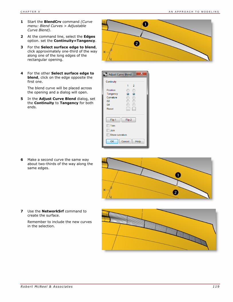
C H A P T E R 9 A N A P P R O A C H T O M O D E L I N G
Robert McNeel & Associates 119
1 Start the BlendCrv command (Curve menu: Blend Curves > Adjustable
Curve Blend).
2 At the command line, select the Edges option. set the Continuity=Tangency.
3 For the Select surface edge to blend, click approximately one-third of the way along one of the long edges of the rectangular opening.
4 For the other Select surface edge to blend, click on the edge opposite the first one.
The blend curve will be placed across
the opening and a dialog will open.
5 In the Adjust Curve Blend dialog, set the Continuity to Tangency for both ends.
6 Make a second curve the same way
about two-thirds of the way along the same edges.
7 Use the NetworkSrf command to create the surface.
Remember to include the new curves
in the selection.


Rober t McNeel & Assoc ia tes 121
10 Applying 2-D graphics Often you are asked to take an existing design from a 2-D graphics package and include it as part of a Rhino model.
In the following two exercises, we will move and position the graphic onto the model.
Exercise 25—Importing an Adobe Illustrator file
In this exercise, we will make a custom construction plane, import an Illustrator file, and place a logo on some surfaces.
1 Open the model Air Cleaner.3dm.
2 In Rhino Options, Modeling Aids, set the Construction planes to use Standard construction planes.
The following techniques will not work if the construction planes are set to use Universal construction planes.
To import a file
1 Start the Import command (File menu: Import).
2 Change the Files of type to Adobe Illustrator (*.ai), and choose the AirOne_Logo.ai to import.
3 In the AI Import Options dialog, click OK.
The logo curves appear at the origin of the Top
construction plane, are selected, and on the Default layer.
Tip: If curves are not planar, use the ProjectToCPlane command (Transform menu > Project to CPlane).
4 While the imported geometry is still selected, use the Group command to group the various curves together. This makes it much easier to select all of the curves and not leave any behind in the following transform steps.
5 Start the Layer command.
6 Turn off the Logo layer in the Layer panel.
7 Right-click on the Logo layer, then click Copy Objects to Layer to
make a copy of the logo on the Logo layer.
We will use this copy later for another part of the exercise.
8 Turn off all the layers except Default and Top Surface.
To create the custom construction plane
We need to set a construction plane to the flat surface. The CPlane command will allow us to do this but the X and Y directions of the new custom construction plane will be mapped to the u- and v-directions of the target
surface respectively. The Dir command will tell you how the u- and v-direction are pointing on the surface, and allow you to change the directions of each.

C H A P T E R 1 0 A P P L Y I N G 2 - D G R A P H I C S
Robert McNeel & Associates 122
1 Select the flat disc shaped surface, then from the Analyze menu, select Direction (Analyze menu:
Direction).
This displays the current surface normal direction and the U/V directions. It is important to know the u- and v-directions of the surface.
The white arrows show the surface normals. A cursor with a red and green arrow appears when you move
over the selected surface.
The red arrow indicates the U direction and the green arrow indicates the V direction.
2 At the command line, notice the options for changing the directions of the surface. You can click on these to change the surface directions. The cursor and surface normals will update accordingly.
When all changes are made, press Enter to accept.
The goal is to have the U and V as in the second image.
In this way, the new construction plane will map to the surface accordingly and the geometry can be mapped to the construction plane predictably.
3 In the Perspective viewport, use the CPlane command with the Object option (View menu: Set CPlane > To Object) or (Viewport title right-click menu: Set CPlane > To Object) to set the construction plane to the
surface.
The x- and y-axes are parallel to the u- and v-directions of the surface as you set them in the previous step.
4 You may want to save the new construction plane with the
NamedCPlane command (Viewport title right-click menu: Set CPlane > Named CPlanes) to make it easy to retrieve later step.
To map the logo curves to the new construction plane
The command we will use to move the logo to the flat disk shaped surface uses the position of the object relative to a construction plane.
1 Select the curves in the Top viewport. Make sure the Top viewport is active, then start the RemapCPlane command (Transform menu:
Orient > Remap To CPlane).
This command depends upon the active construction planes at each stage, so it is important to pick in the correct viewports.

C H A P T E R 1 0 A P P L Y I N G 2 - D G R A P H I C S
Robert McNeel & Associates 123
2 Click in the Perspective viewport with the custom CPlane.
You could use the Copy=Yes option in this command so that a copy is
remapped instead of the original.
The logo is positioned in the same relative position on the custom construction plane as it was in the active viewport.
3 Rotate, Move, or Scale the logo to a new position.
For an accurate view of the surface and the curves, you may want to use the Plan command in the Perspective viewport. This sets the view to a parallel projection looking straight on at the plane.
4 Use the ExtrudeCrv command (Solid menu: Extrude Planar Curve > Straight) with the BothSides option to make the text 3-D. The extrusion distance should be 1 mm.
5 Use the BooleanDifference command (Solid menu: Difference) to
recess the text into the surface.
Exercise 26—Flow the logo onto a freeform surface with history
In this part of the exercise, we will use the copy of the logo that is on the Logo layer and position it on the cutout surface. This surface is not flat so we will use a different transform tool, Flow along Surface, to move it and
bend it along the surface. Flow along Surface morphs objects from a source surface to a target surface. It uses the UV of the surfaces to determine how it flows. It is important that the source and target surfaces have the same relative UV direction.
To make the base surface
1 Start the Layer command and make the Cutout layer the current layer. Then, turn off all the layers except Cutout and Logo.
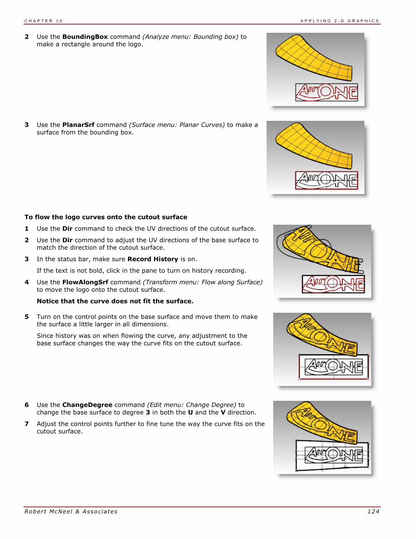
C H A P T E R 1 0 A P P L Y I N G 2 - D G R A P H I C S
Robert McNeel & Associates 124
2 Use the BoundingBox command (Analyze menu: Bounding box) to make a rectangle around the logo.
3 Use the PlanarSrf command (Surface menu: Planar Curves) to make a
surface from the bounding box.
To flow the logo curves onto the cutout surface
1 Use the Dir command to check the UV directions of the cutout surface.
2 Use the Dir command to adjust the UV directions of the base surface to match the direction of the cutout surface.
3 In the status bar, make sure Record History is on.
If the text is not bold, click in the pane to turn on history recording.
4 Use the FlowAlongSrf command (Transform menu: Flow along Surface)
to move the logo onto the cutout surface.
Notice that the curve does not fit the surface.
5 Turn on the control points on the base surface and move them to make the surface a little larger in all dimensions.
Since history was on when flowing the curve, any adjustment to the
base surface changes the way the curve fits on the cutout surface.
6 Use the ChangeDegree command (Edit menu: Change Degree) to
change the base surface to degree 3 in both the U and the V direction.
7 Adjust the control points further to fine tune the way the curve fits on the cutout surface.

C H A P T E R 1 0 A P P L Y I N G 2 - D G R A P H I C S
Robert McNeel & Associates 125
To raise the logo lettering and flow it onto the cutout surface
1 Use the ExtrudeCrv command with the BothSides option to make the
text 3-D. The extrusion distance should be 1 mm.
2 Use the FlowAlongSrf command to move the solid logo onto the cutout surface. Use the new base surface.
History is not needed this time, since all the needed adjustments were already done on the base surface.
3 Use the BooleanUnion
command to join the logo with the cutout surface.

C H A P T E R 1 0 A P P L Y I N G 2 - D G R A P H I C S
Robert McNeel & Associates 126
Make a model from a 2-D drawing
One of the more difficult modeling tasks in modeling is to interpret a set of 2-D
views into a 3-D model. Very often, the drawings are precise in some areas and inexact in areas where complex surface transitions must take place in three dimensions.
It is best to consult directly with the designer to clarify difficult areas, but this is not always possible. Usually there are discrepancies between the views.
If there is no physical model available as reference, some decisions must be made along the way about the best way to interpret the control drawing. For example, you will have to consider which view to consider the most accurate for a given feature.
In the following exercise, we will explore some strategies to create a blow-molded plastic bottle from a set of 2-D drawings. In this exercise, we have a control drawing showing three views of the bottle. It is roughly dimensioned, but we need to hold to the designer’s curves wherever possible.
We will only have time to finish the first stage of this model in class. We will complete the bottle surfaces, but the details will be left out. Included in the models folder is a finished bottle for your review.
Control drawing
Exercise 27—Making a detergent bottle
To group the parts
1 Open the model Detergent Bottle.3dm.
2 In the Top viewport, window select the objects that make the top view (lower left) including the dimensions of the 2-D drawing.
3 Use the Group command to group the selected objects (Edit menu: Groups > Group).
4 Repeat the previous steps to group the objects for the front view (upper
left) and the right view (upper right).
Each of the views is a separate group of objects.
To orient the Top view
1 Select the top view group.
2 Use the ChangeLayer command (Edit menu: Layers > Change Object
Layer) to change the layer to the 2D Template Top layer.
3 In the Top viewport, use the Move command to move the center of the circles to 0,0.

C H A P T E R 1 0 A P P L Y I N G 2 - D G R A P H I C S
Robert McNeel & Associates 127
To orient the Front view
1 Select the front view group.
2 Use the ChangeLayer command to change the layer to the 2D Template Front layer.
3 In the Top viewport, use the Move command to move the intersection of the centerline and the horizontal line at the bottom to 0,0.
4 While the front view group is still selected, start the RemapCPlane command (Transform menu: Orient > Remap to CPlane) in the Top viewport.
5 Click in the Front viewport.
The view is oriented in 3-D space.
To orient the Right view
1 In the Top or Perspective viewport, select the right view group.
2 Use the ChangeLayer command to change the layer to the 3D Template Right layer.
3 In the Top viewport, use the Move command to move the intersection of the centerline and the horizontal line at the bottom to 0,0.
4 Use RemapCPlane to map the right view curves to the Right construction plane.
The view is oriented in 3-D space.
Frequently 2-D curves for design control drawings will not be as carefully constructed as you like for making accurate geometry. Before building 3-D geometry from the 2-D curves, check the curves and correct any errors
that can be found.
To create the 3-D curves
The inset part of the bottle will be cut into the surface later. For the moment, we just need to build the outer surfaces. The fillets at the top and bottom indicated in the curves can be left out of the initial surface building and added in as a separate operation. We will need to extend or redraw the edge curves to bypass the fillets and meet at hard corners before making the surfaces.

C H A P T E R 1 0 A P P L Y I N G 2 - D G R A P H I C S
Robert McNeel & Associates 128
Several surfacing tools could be used to build the initial surfaces: A 2-Rail Sweep or a Surface from Network of Curves are the obvious choices.
Network surfaces do not pay any attention to the curve structure, only the shape. All curves are refit and the
resulting surface has its own point structure.
Other commands including the Sweep tools, lofting and edge surfaces do pay attention to the curve structure in at least one direction. In these cases, it often pays to use matched curves as cross sections. The choice of surfacing tools may well determine the way in which the actual input curves are created.
1 Select the groups you made in the previous step, use the Ungroup command (Edit menu: Groups > Ungroup) to ungroup them.
2 Select the curves from each 2-D template view that define the outer surface and Copy them to the 3D Curves layer.
Since the bottle is symmetrical on both sides of the X-axis, you will only need to copy the curves on one side. They will be mirrored later.
3 Use the OneLayerOn command (Edit menu: Layers > One Layer On) to set the 3D Curves layer.
4 Move the curve defining the top surface of the bottle to the same height as the top of the vertical curves.
Use SetPt or Move with the Vertical option in the Perspective view.
5 The vertical curves now can be extended past the fillet curves so that they meet the top and bottom curves exactly on the endpoints of these curves.
One way is to extend the vertical curves using Extend with Type = Smooth. Snap to the End or Quad points of the top curve and the base curve at the bottom.
Extending the curves in this way will add complexity to the curves. If it is important to keep the curves simple and well matched, it may be better instead to adjust the points on the existing curves to extend them.
6 Undo the Extend operation, and instead point edit the curves directly.
You can make a duplicate set of curves and edit one of each leaving the original in place as a template.
7 Mirror the base, top and side curve visible from the right view to the other side.
The result should be a set of 8 curves that define the surface.
Most of these curves are essentially the original curves from the 2-D drawings but rearranged in 3-D.

C H A P T E R 1 0 A P P L Y I N G 2 - D G R A P H I C S
Robert McNeel & Associates 129
8 Join the base curves and the top curves into a closed loop.
The curves are set up for a surface from a curve network or a two-rail sweep.
To make a surface for the bottle with a sweep
From the drawing these are the only curves we have available to define the shape, so we will use these curves directly to create the surface.
1 Change to the Surfaces layer.
2 Window select the curves, and try Sweep2 to make a surface then Shade the viewport.
Notice the shape gets severely out of control at the rounded side of the bottle.
3 Move this surface to the side for the moment.
While it is possible to rearrange or
add curves to make the Sweep2
work better, it is worth checking how a surface from a Curve Network will work with the same set of curves.
4 Select all of the curves, again, the use the NetworkSrf command to
create the surface.
The NetworkSrf command handles this set of curves much more gracefully.
On your own
Make the inset surface and the handle.
Fillet the edges where indicated in the 2-D drawing.
Included in the model directory is a finished bottle, Finished Detergent bottle.3dm, for
your review.


Rober t McNeel & Assoc ia tes 131
11 Surface analysis Rhino has several tools to help you visually evaluate surface quality. In this exercise, we will use curve and surface analysis tools to help build clean, simple surfaces with good continuity.
Some models require more attention to continuity, primarily, because it will show when manufactured. For example, a blow-molded bottle will not show slight inconsistencies in the surface, but a car panel will.
Exercise 28—Surface analysis
The file, Surface Analysis.3dm, has a set of curves you will recognize from the previous exercise. Our task in the current exercise is to make curves that can create cleaner, simpler surfaces with good continuity. We will
make use of the CurvatureGraph, Zebra, and CurvatureAnalysis to make sure we set things up for the best results. Lastly, we will compare the surface analysis results in this file with the surface analysis results in the previous exercise.
To evaluate the curves
First, let us look at the curvature graphs of the top and the bottom curves. These curves have a nice enough
shape, but there is room for improvement from a surfacing continuity perspective.
1 Select the top and bottom curves.
2 Start the CurvatureGraph command (Analyze menu: Curve > Curvature Graph On) and set the Display scale to a value of 120.
The graph tells us that both curves are tangent continuous but have curvature discontinuities in a couple of locations.
Assuming we want the surfaces we build from these curves to have curvature continuity throughout, we will be better off modifying these curves before
creating the surfaces.
If we decide ahead of time what the surface arrangement will be, that will help us understand how to draw clean new curves.
Building a surface that has consistent curvature as a single surface is good modeling practice. Looking at the bottom curve, we can see two areas that are good candidates for creating the surfaces, so we will start there. There is an area of high curvature at the front (1) and a relatively flat stretch in the
middle with a rapidly increasing curvature at the handle side (2). The top curve is smoother overall, but has similar corresponding regions of curvature.
By examining the current curves, we can identify two curves to build at the top and bottom. The white vertical curve intersects the top and bottom curves at the curvature discontinuity of the top curve, which is a modified circle, and on an abrupt change in curvature on the lower curve. This intersection is where we will start and end our modified curves.
To build the modified curves
1 Using the current curves as a reference, draw four new curves of degree five with six points.
The goal is to redraw the top and bottom curves in two parts each.
Keep in mind what you know about continuity, CurvatureGraph, tangent directions, and EndBulge.
Try to keep the control point locations even and progressive.

C H A P T E R 1 1 S U R F A C E A N A L Y S I S
Robert McNeel & Associates 132
2 Analyze your curves with the CurvatureGraph command.
Try to get the graph clean with minimal, abrupt changes, while at the same
time match the original curve shapes as closely as possible.
They cannot be exactly the same as the originals if they are to have better continuity, but it should be possible to get close.
To make the surfaces for the bottle from edge curves
There are four, single-span, curves that define each area for the surfaces. In this part of the exercise we will use the EdgeSrf command (Surface menu >
Edge curves) to create the surfaces. This command
is one that uses the input curve structure to create the surface. It works best if the curves on opposite sides of the rectangle match each other. The resulting surface will be simpler.
Since we have taken care to meet this criterion, all of the vertical curves are degree 3 with four points,
and the curves we just made are degree five with six points, the resulting surfaces will share this structure.
1 Select four curves that define one of the surfaces.
2 Start the EdgeSrf command (Surface menu >
Edge curves).
3 Repeat steps 1 and 2 for the other surface.
4 Check the surfaces with the Zebra command.
The zebra stripes have a nice even flow but the surfaces are clearly not tangent at the vertical edge.

C H A P T E R 1 1 S U R F A C E A N A L Y S I S
Robert McNeel & Associates 133
To match the surfaces for the bottle with MatchSrf
1 Use the MatchSrf command (Surface menu: Surface Edit Tools > Match) to match the surfaces for Curvature. Try matching in both directions, and with or
without Average surfaces set.
In this case, the results are good no matter how the match is made, but it is worth looking at the control points on the surfaces in each case.
Matching the larger surface to the smaller one, without Average, results in a more erratic control point arrangement on the larger surface than any other combination, particularly the second row from the top. Other considerations being equal, the best choice is the surface with the most regular, even control
point arrangement.
2 Check the surfaces with the Zebra command.
The zebra stripes have a nice even flow with no discontinuity at the common edge.
To match the surfaces for the bottle with Symmetry
In this section, we will make the other half of the bottle using the Symmetry command with Record History turned on. Symmetry mirrors curves and surfaces, makes the mirrored half tangent to the original, and with History recording active, when the original object is edited, the mirrored half updates to match the original.
1 Select the larger surface.
2 Use the Symmetry command (Transform menu: Symmetry) to mirror the surface across the x-axis. Make sure Record History is on.
3 For the Select curve end or surface edge, select the edge of the surface (1).
4 For the Start of symmetry plane, type 0 and press Enter.
5 For the End of symmetry plane, use Ortho to pick a point along the x-axis.

C H A P T E R 1 1 S U R F A C E A N A L Y S I S
Robert McNeel & Associates 134
6 Repeat this process for the other surface.
If you edit either original surface, the mirrored part will update to match.
7 Check the surfaces with the Zebra command.
The zebra stripes have a nice even flow with no discontinuity at the common edge.
To analyze the matched surfaces
At this point, we will use the Curvature Analysis tool to evaluate the matched surfaces. This can be useful in locating areas of extreme curvature, but may force the display to ignore more subtle changes. In any case, the
display on each of these simple surfaces should be very smooth and clean.
1 Hide all curves to get a good view of the transitions between surfaces.
2 Select all of the surfaces and turn on Curvature Analysis display (Analyze menu: Surface > Curvature Analysis).
Set the style to Gaussian, and click Auto Range. Make sure you have a fine analysis mesh for a good visual evaluation. Click back and forth
between Auto range and Max range.
Auto Range attempts to find a range of color that will ignore extremes in curvature, while Max Range will map the maximum curvature to red and the minimum to blue.
The numbers are for Curvature, which is, 1/radius.
The goal when matching is to maintain as even and gradual a curvature display as possible, while meeting the continuity requirements.
Notice the edges that have been matched appear to have a smooth color transition.

C H A P T E R 1 1 S U R F A C E A N A L Y S I S
Robert McNeel & Associates 135
To analyze and compare different surfacing techniques
Next, we will make another surface for comparison.
1 Copy the curves to one side.
2 Mirror and Join the top and base curves on the x-axis.
3 Mirror the vertical side curve on x-axis to make a set of curves suitable for a surface form a curve network.
4 Use NetworkSrf to make a surface from these curves. Select the new surface and Add it to the Curvature Analysis display.
The denser network surface (2) has a less clean appearance in
this display. The simple surfaces (1) still look cleaner at this point.
Since the color change is mapped across the entire range shown, it is important to remember that the Auto Range setting indicates a very narrow range of curvature and that the actual
differences may be small even though the color change is great.


Rober t McNeel & Assoc ia tes 137
12 Sculpting Designers can build a relatively undefined surface and then use a variety of transform and analysis tools to sculpt a surface in 3-D space in an intuitive and direct manner—design “as you go.”
Place curves approximately. The curves should be edited copies of a single original if possible.
This ensures that they will be compatible when lofted, and create the simplest, most easily edited surface.
Start with the big changes and then make the detailed changes.
Use the IncrementalSave command to make copies of the model as you progress.
In the following exercise, we have created four curves for you to use. They describe a very simple dashboard
from which to start your design. An added steering wheel, on a locked layer, is to help you get a sense of scale and positioning of any elements you might wish to add.
Tools to help in control point editing
Move Control Points by dragging, using the Move, Rotate, or Scale commands or other Transform commands.
Dragging, of course, is the most fluid and interactive way to edit the shape. However, there may be situations
where the construction plane constraint for point movement is less than optimal. Here are some tools that can help with control point editing:
Gumball
Gumball works very well with control points. It is convenient to be able to switch easily among the various gumball orientation modes. Opening the Gumball toolbar will help.
When Gumball orientation is set to Align to Object, the blue axis orients itself to the surface normal for a selected control point. By dragging the blue arrow, the control point moves in the local surface normal direction. The red axis aligns to the surface U direction. Make fine adjustments by setting the Gumball drag strength to something less than 100%.
DragMode
DragMode lets you override the current construction plane constraints in several ways.
Command-line options
World
This constrains dragging as if the CPlane were always World Top. This is rarely used.
CPlane
The default constraint in Rhino. Dragging takes place parallel to the active CPlane.

C H A P T E R 1 2 S C U L P T I N G
Robert McNeel & Associates 138
View
Dragging takes place parallel to the current viewport. This can be useful in some oblique views.
UVN
Dragged surface control points with Ortho on (Shift key) are constrained to the surface u- and v-directions and with the Ctrl key are constrained to the surface normal direction. Curve points are constrained to the curve tangent and with Ctrl to the curve normal direction. For this exercise, this is most useful drag mode.
ControlPolygon
This mode constrains dragged curve and surface control points to the control polygon. In the case of multiple selected points, each moves along its own control polygon. This is an excellent tool for keeping points well organized in rows and columns.
As with the Gumball, having the DragMode toolbar open makes it easy to switch among modes while point editing. Notice the cursor changes to reflect the current drag mode. In general, you will probably find it easier to switch the Gumball off when dragging points using the special drag mode options.
MoveUVN
This tool opens a dialog box that allows you to move control points in increments according to a user set scale. The point movement can be along the U, V, and N (Normal) directions. In addition, there are smoothing tools in this dialog. These are very useful for smoothing out bunched or irregular control points to achieve a more
regular grid.
Nudge
Use the arrow keys with Alt, Alt+Shift and Alt+Ctrl to move points in small increments. Note the settings in the
(Options > Modeling aids > Nudge page) allow you to set the Nudge constraints similarly to some of the DragMode settings mentioned above.
Tip: You can use the knowledge gained in the User Interface portion of this course to create macros that make it easy to swap among the nudge modes.
SetPt
This allows you to true up points or rows of points in one, two, or all three dimensions.
Use any or all of the above tools to manipulate the surface points individually and in groups. Keep in mind the point selection tools: SelU, SelV and others in the Select Points toolbar.
You will see that with a relatively sparse set of control points, as we have on this starting surface, the edits you make tend to be large ones that affect the shape broadly. It is likely that you run out of control quickly.
In this case, you will find that you need have more localized control to add smaller details. You can add control by increasing the density of the control points. There are two similar tools for this:
InsertKnot
Inserts one or more knots, and rows of control points. Surface points are rearranged so that the shape of the surface does not change. In other words, except in special cases, the new points are not added at the same location as the new knot.
InsertControlPoint
Allows you to place the row of points where you want them to be, however the mechanism for adding these points
does nothing to ensure that the shape of the surface stays the same. Generally, the shape will change.
Both InsertKnot and InsertControlPoint have advantages, but when you are making heavily curved and
sculpted surfaces, InsertKnot may be the safer choice since it does not change the shape of the surface.
Some considerations when inserting knots
Insert as few knots as you can to get the control you need. Add more later if needed. Keep the surface as simple as possible while getting the control you need.
Where possible, insert knots so that they are as evenly spaced as possible. Try to place them halfway between existing knots.

C H A P T E R 1 2 S C U L P T I N G
Robert McNeel & Associates 139
Command-line options
Automatic
Adds knots halfway between existing knots to maintain as uniform a structure as possible. It increases the
knot density of a curve or surface, and thus the control point density as well, while maintaining an even knot distribution, which makes point editing more predictable than with unevenly spaced knots. Be careful with this option, as it adds a knot between each pair of existing knots, so a surface can become very dense in structure very quickly.
MidPoints
Places markers halfway between the existing knots/knot lines that can act as guides for inserting knots midway between existing knots. Use the Point object snap to place new knots at these markers.
Note: It is easy to get to a point where there are too many control points and you simply lose control of the
shape. Therefore, it is a good idea, to use IncrementalSave before adding complexity to the object. This
will allow you to go back to a simpler model without starting over if things get out of hand.
Exercise 29—Dashboard
1 Open the model Dash.3dm.
2 Loft the four curves together with the Loose option from the dropdown list.
Using the Loose style creates the simplest possible geometry and is essential to creating a surface with this technique. The surface will not touch the interior curves of the loft
with this option, but it should be very smooth and clean looking.
3 Turn on the control points.
If you also turn on points for the input curves, you will see that the point
structure of the surface exactly matches that of the four curves.
4 Turn off the Curves layer.
You can do at this point to sculpt the shape. The most obvious one is simply to move the surface control points around, so let us start there.
As mentioned, Rhino has several powerful tools to help in control point editing.
To edit and sculpt the surface
1 Turn on the points for the surface, with Gumball off for the moment.
2 Window select the three control points that are just to the right of the steering column centerline.
3 Use the SetPt command (Transform
menu: Set XYZ Coordinates) to align the groups of points in the x direction in Top or Front snapping to the centerline.
Notice that when the points are selected, there is a red and a green line extending from the selected points- this indicates the positive u- and v-directions.

C H A P T E R 1 2 S C U L P T I N G
Robert McNeel & Associates 140
4 Use this information with the point selection tools NextU, NextV,
PrevU, or PrevV to shift the selection
to the left or right to the next row of points. SetPt these points to the corresponding edge, left and right, of the steering wheel.
5 Use Gumball to drag the lowest three points near the steering wheel down
to accent the shape.
The shape may not be symmetrical compared to the steering wheel.
6 Select the points nearest the top edge of the steering wheel and set them all to the same Z using SetPt.
7 Now, let us add some definition to the
dash in the area of the steering wheel. Set the DragMode to ControlPolygon, and drag three of the points up very close to their neighbors.
The shape of the surface changes only slightly. It is still very soft, and there are no more points available to continue to edit there.
8 Use the InsertKnot command (Edit menu: Control Points > Insert Knot)
to add a row of points in the V direction.
The surface currently has no interior knots so use the Automatic option once to add a single knot.
Now, with the extra points you can continue to slide points along the control polygon to sharpen up the surface in this area.
9 Use the IncrementalSave command (File menu: Incremental Save) before going on to the next step.
10 Another way to tweak the shape is to
set the point weight of some of the points on the surface. For example, select the three middle points that are at the apex of the now sharply curved area we have been editing. Start the Weight command (Edit menu: Control Points > Edit Weight).
Increase the weight of the points to 2.
Higher weight points, relative to neighboring points, tend to pull the surface toward them. Lower weight points cause the surface to fall away from the control points.

C H A P T E R 1 2 S C U L P T I N G
Robert McNeel & Associates 141
To add and manipulate knots
Try inserting knots in either direction, using the Midpoints=Yes setting to be able to snap to span midpoints. Insert some knows with Midpoint=No to insert knots close to existing ones to allow more local control.
1 Use the IncrementalSave command (File menu: Incremental Save) before going on to the next step.
2 Use InsertKnot, Midpoints=Yes, to insert some knots in the U direction. Snap to midpoints to keep knot spacing even.
Notice how the control point arrangement changes with each knot inserted. You may want to true up some rows of points in X using SetPt
to keep the rows and columns organized.
3 Explore different shapes and design ideas using all of the tools mentioned above.
4 Select some points that are out of alignment. Start the MoveUVN
command (Transform menu: MoveUVN). Use the Smooth sliders to
smooth some of the points that are out of alignment.
5 Move some points to the right of the steering wheel closer to it to make the shape more symmetrical about the steering wheel.
Where possible, try to keep the control point arrangement even and progressive. As you might expect, there tend to be more control points
in areas that have been edited and shaped the most.
6 Add some more knots in the area of the top of the steering wheel.
If you crowd a few knots in this area, you can pull out a localized feature that fades smoothly into the surrounding surface.
To make the offset surface
When you are satisfied with the overall shape of the surface, you can add details to make a more finished object.
The surface can be offset and trimmed as in the first illustration.
Best results are obtained when the surface has at least degree 3 in both directions. Check this with Object Properties.

C H A P T E R 1 2 S C U L P T I N G
Robert McNeel & Associates 142
Note: Offsetting surfaces generally results in a surface of one step lower in internal continuity. Surfaces that are
only G1 internally may result in surfaces that have G0 continuity; that is, they may have a kink in them. Although Rhino allows these surfaces, this can lead to problems downstream.
For this reason, if you intend to offset surfaces, it is best where possible to create the initial surface from degree 3 or higher curves. These surfaces have at least G2 continuity so that offsetting them will result in at least G1 continuous surfaces. Changing the degree of a surface that has been created from degree-2 curves to at least degree 3 in both directions is not sufficient to ensure a G2 surface. Simply changing the
degree after the fact does not improve internal continuity.
1 Change to the Cutting Curves layer.
2 Draw a curve that represents where you want to split the surface.
3 Use the Offset command (Curve menu: Offset Curve) to make a
duplicate of the curve offset by one-
half (0.50) inch.
4 Use the Trim command (Edit menu: Trim) to trim the surface between the curves.
5 Use the OffsetSrf command (Surface menu: Offset Surface) to offset the back surface by one-fourth (0.25) inch.
6 Delete the original surface.
7 Use the BlendSrf command (Surface menu: Blend Surface) to blend between the two surfaces. Set edge 1 to Curvature (G2) and edge 2 to Position (G0).
One of the things we are trying to
show here is a quick way to make a “tucked” upholstery type transition.
Adjust the BlendSrf sliders so the cross-section looks like the example on the left.

C H A P T E R 1 2 S C U L P T I N G
Robert McNeel & Associates 143
8 Add details if time allows.


Rober t McNeel & Assoc ia tes 145
13 Deformation tools Deformation tools allow you to deform meshes, lines, surfaces, polysurfaces, and solids without worrying about the integrity of the object.
Start the deformation commands from the Transform menu, or from the Deformation Tools toolbar:
Icon Command Description
FlowAlongSrf Morphs objects from a source surface to a target surface.
Splop Copies, rotates, scales, and wraps objects on a surface, like pottery sprigging or appliqué.
OrientOnSrf Moves or copies and rotates objects on a surface using the surface's normal direction for orientation.
Maelstrom Deforms objects in a spiral.
Stretch Scales selected areas of an object in one direction.
Twist Deforms objects by rotating them around an axis.
Bend Deforms objects by bending along a spine arc.
Taper Deforms objects toward or away from a specified axis.
Flow Re-aligns an object or group of objects from a base curve to a target curve.
CageEdit Deforms objects smoothly using one-, two-, and three-dimensional cages.
Cage Creates a box-shaped cage object to be used with the CageEdit command to deform other objects.
ReleaseFromCage Removes selected objects from the influence of a control object set up by the Cage or CageEdit command.
Deforming objects
Exercise 30—Using cage editing to deform an object
To deform an object with CageEdit
1 Open the model CageEdit_Mug.3dm.
2 Open the Cage toolbar.

C H A P T E R 1 3 D E F O R M A T I O N T O O L S
Robert McNeel & Associates 146
3 Start the CageEdit command (Transform menu: Cage Editing > Cage Edit or Cage toolbar) and select the mug as the captive object.
4 For the control object, choose BoundingBox and then World.
5 Specify four cage points and degree 3 in each direction.
The degree can be set up to degree 9. The point count must be greater than the degree value in each direction.
6 For the Region to edit, choose Global.
The deformation of captive objects will take place throughout 3-D space and will not end at the edges of the cage. This setting is important if
some of the captive objects are outside of the cage.
7 Move the control points on the top of the cage vertically to deform the mug.
Cage points can be moved, dragged, scaled, sheared, rotated, bent, etc.
To limit the region to edit
To deform the handle only, a cage object is needed around the just the handle.
1 Use ReleaseFromCage (Cage toolbar) the mug from the cage object. Delete the cage.
2 Start the Cage command and create a freestanding cage object.
3 Move the cage into place and Scale it before attaching it to the mug
4 Start the CageEdit command.
5 For the Select captive object, select the mug.
6 For the Select control object, select the pre-positioned cage object.
7 For the Region to edit, choose Local and set a Falloff distance to 5.
This tells Rhino that the distortion of the cage will affect only the region inside the cage, plus a smooth falloff effective over 5 units moving out from the cage itself.
8 Move the two right-most vertical rows of cage points slightly to the right
in the Front view to increase the size of the handle.

C H A P T E R 1 3 D E F O R M A T I O N T O O L S
Robert McNeel & Associates 147
To CageEdit with a surface from the object
While it is possible to use any curve or surface as a control object in CageEdit, there are many cases where the most intuitive solution is to use a curve or surface that is already part of the object.
The CageEdit command lets you select a surface, including a surface from the captive object, to use as control object.
1 Open the model Salad_Cage.3dm.
2 Select the salad fork and start CageEdit.
3 For the Control object, click on the top surface of the fork.
A copy of the surface is extracted from the object and turned into a
control object.
4 Accept the defaults for the
subsequent options.
5 When the control points are on, move the five points nearest the end vertically.
This gives the fork a little more bend to the front of the fork.
6 Undo.
To CageEdit with a curve from the object
A curve can also be used as a control object. In many cases, it makes sense to use a curve that already has the same basic shape as the object. You can draw such a curve or extract an isocurve from the object itself and use this as the control.
1 Re-open the model Salad_Cage.3dm without saving.
The red curve is an extracted isocurve from the bottom surface that has been extended slightly at each end.
2 Select the salad fork and start CageEdit.
3 Select the red curve as the Control object.
4 Edit the shape of the fork by point editing the Control object.

C H A P T E R 1 3 D E F O R M A T I O N T O O L S
Robert McNeel & Associates 148
Exercise 31—Using other deformation tools
To stretch an object
The Stretch command allows you to scale a selected area of an object in one direction.
1 Open the model StretchWrench.3dm.
2 Select the wrench.
3 Start the Stretch command (Transform menu: Stretch).
4 For the Start and End of axis, snap to the two locked points.
5 For the Point to stretch to, pull the
cursor to one side or another to
stretch or compress the wrench.
The section of the wrench that falls between the points that set the stretch axis is the part that is deformed. The object outside of this initial axis is moved, but not
deformed. The shape of working parts of the wrench at either end are not affected, but the overall object is made longer or shorter.
To place a small detail on an object
Here the goal is to place the small detail that is off to the side of the cup onto the cup handle. The detail is easy
enough to build in a flat, orthographic orientation but would be quite tedious to build accurately in place on a curved surface.
The OrientOnSrf command can place an object on an arbitrarily curved and oriented surface with good control over the placement and can optionally also deform the object to match the curvature of the target surface.
1 Open the model OrientOnSrf_detail.3dm.
2 Start OrientOnSrf, and select the detail object.
3 For the Base point, snap to the point marked 1.
This will be the point that is placed on the target surface.
4 For the Reference point, snap to the point marked 2.
This point and the line between it and the base point will be used to set
scaling and orientation on the target surface. The current CPlane Z direction will be mapped to the target surface normal.
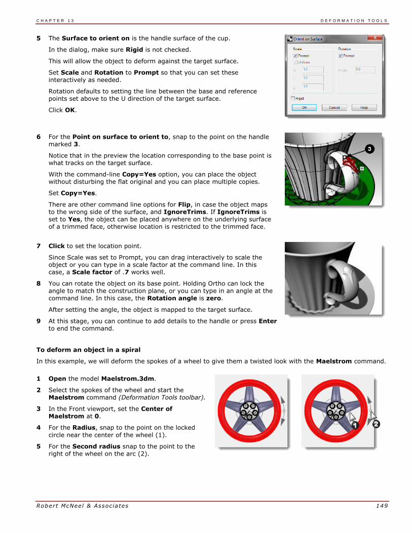
C H A P T E R 1 3 D E F O R M A T I O N T O O L S
Robert McNeel & Associates 149
5 The Surface to orient on is the handle surface of the cup.
In the dialog, make sure Rigid is not checked.
This will allow the object to deform against the target surface.
Set Scale and Rotation to Prompt so that you can set these interactively as needed.
Rotation defaults to setting the line between the base and reference points set above to the U direction of the target surface.
Click OK.
6 For the Point on surface to orient to, snap to the point on the handle marked 3.
Notice that in the preview the location corresponding to the base point is what tracks on the target surface.
With the command-line Copy=Yes option, you can place the object without disturbing the flat original and you can place multiple copies.
Set Copy=Yes.
There are other command line options for Flip, in case the object maps to the wrong side of the surface, and IgnoreTrims. If IgnoreTrims is set to Yes, the object can be placed anywhere on the underlying surface of a trimmed face, otherwise location is restricted to the trimmed face.
7 Click to set the location point.
Since Scale was set to Prompt, you can drag interactively to scale the object or you can type in a scale factor at the command line. In this case, a Scale factor of .7 works well.
8 You can rotate the object on its base point. Holding Ortho can lock the angle to match the construction plane, or you can type in an angle at the command line. In this case, the Rotation angle is zero.
After setting the angle, the object is mapped to the target surface.
9 At this stage, you can continue to add details to the handle or press Enter to end the command.
To deform an object in a spiral
In this example, we will deform the spokes of a wheel to give them a twisted look with the Maelstrom command.
1 Open the model Maelstrom.3dm.
2 Select the spokes of the wheel and start the
Maelstrom command (Deformation Tools toolbar).
3 In the Front viewport, set the Center of Maelstrom at 0.
4 For the Radius, snap to the point on the locked
circle near the center of the wheel (1).
5 For the Second radius snap to the point to the right of the wheel on the arc (2).

C H A P T E R 1 3 D E F O R M A T I O N T O O L S
Robert McNeel & Associates 150
6 For the Coil angle, drag the cursor around the circle about 15 degrees to deform the spokes into a
soft spiral shape.
To deform an object by flowing it along a curve
In this example, we will flow an object along a curve while recording history. This will allow us to do a secondary deformation of the original object and see the update on the flowed piece.
1 Open the model Flow & Twist.3dm.
2 On the Status bar, turn Record History on.
3 Right-click the Record History pane, and select the Update Children checkbox.
4 Select the polysurface and start the Flow command (Transform menu:
Flow Along Curve).
5 Set Copy=Yes, Rigid=No, Local=No, and Stretch=Yes.
6 For the Base curve select the straight line (through the center of the polysurface).
7 For the Target curve, select the circle.
A copy of the polysurface flows around the circle.
8 Select the original polysurface, and start the Twist command (Transform menu: Twist).
9 Twist the original polysurface 360 degrees, using the straight line as the twist axis.
The polysurface created with the Flow command and History updates to match the twisted polysurface.

Rober t McNeel & Assoc ia tes 151
14 Blocks There are two main advantages to using blocks in Rhino:
Identical objects can be edited or replaced at the same time.
Since many identical objects refer to one definition, files with many repeated objects can be smaller, sometimes much smaller, than files where each of those is its own independently defined object.
In Rhino, a block appears as a collection of objects. These can be simple 2-D or complex 3-D objects. A block can be composed of lines, polylines, freeform curves, surfaces, polysurfaces, solids, dimensions, text, and even other blocks. When a block contains other blocks, these are said to be nested. The level of nesting that may be used is
not limited.
Instances and definitions
Each block has a single definition. The definition is the set of objects that comprise the block. This definition is hidden from the user. Its purpose is to provide the definition for the instances of the block that appear in the model. There can be any number of instances of a block, but only one definition. Thus, when the user modifies a
block definition, all of the instances of that block will reflect the changes.
Defining blocks
Blocks can be defined using the Block command. This adds a new block definition and leaves one instance of the
block in place.
Block instances can be added by copying existing instances, or by using the Insert command. Insert allows you to choose from a list of existing block definitions, or to browse to an external file.
Note: There may be block definitions in a file for which no instances appear. Deleting an instance does nothing
to the definition.
Insertion points
Each block has an insertion point. This is a base location for the block as a whole and is in fact the point used when a block instance is added using the Insert command.
Embedded and linked blocks
When the definition of a block is saved in the Rhino file, the block is said to be embedded. If the block definition exists as a separate file, the block is linked. In the latter case, saved changes to the external file are what govern the appearance of the block instances in all of the files into which it is inserted.
Layers and blocks
Layers can be confusing when using blocks. It is important to keep in mind that any instance of a block will exist on some layer just like any Rhino object. Typically, this is the layer that is current when the instance is inserted, but the instance layer can be changed, just like any other type of object. However, each object in the block definition also exists on some layer, independent of the block instance as a whole. For example, two instances of the same block can be on different layers, but the objects comprising the block definition will be on the same
layers in each instance.
Turning on or off a layer containing an instance will show or hide the entire instance. Turning on or off layers of the objects contained in a block will show or hide that part in every instance of the block, regardless of what layer the instance is on.
Linked blocks' layers (reference layers) can be shown in the layer panel as normal layers, or displayed as special reference layers.
Here are some rules that are good to keep in mind when using blocks:
The layer that is current when the block instance is inserted is called the reference layer. The inserted instance resides on this layer.
The visibility of the entire block is controlled with the block reference layer.

C H A P T E R 1 4 B L O C K S
Robert McNeel & Associates 152
If you turn the block reference layer off, the entire block will not be visible, regards less of the layers to which the geometry is assigned.
Objects in the block that have properties assigned by parent; will have a unique behavior when grouped
together in a block.
Object properties of display color, plot color, and plot width can be assigned by parent.
Objects assigned by parent and grouped into a block have a chameleon-like property. They change to display the color and the plot weight of the block’s reference layer.
This powerful feature allows a block to look different, without creating a separate block.
The layer that is current when the block is made does not have any bearing on the block definition itself. The layers of the objects in the block definition, and the layer that is current when an instance is inserted
are important in how the block instances behave with respect to visibility.
Editing blocks
Block definitions are most easily edited using the BlockEdit command, or by double-clicking on a block instance. If the block is a linked block, editing will open the linked file in a new instance of Rhino and the current Rhino will
be suspended until that second Rhino is closed.
Exercise 32—Block basics
To make a block
1 Start a new model.
2 Draw a box and a sphere somewhere near the origin.
3 Select the two objects
4 Use the Block command (Edit menu: Blocks > Create Block Definition) to make a block.
5 For the Block Base Point, snap to a
corner of the box.
The point you select will become the insertion point for the block.
6 In the Block Definition Properties dialog Name field, type Test 1, press OK.
7 Use the Insert command (File menu: Insert) to insert the new block.
8 In the dropdown list at the top of the Insert dialog, select Test 1.
Make sure to insert as Block Instance and not as a Group or Individual Objects. Accept the defaults for Scale and Rotation.
9 Place the block in the Rhino scene.
Notice that the cursor follows the location that you set as the block base
point when the block was created. This is the insertion point.

C H A P T E R 1 4 B L O C K S
Robert McNeel & Associates 153
10 Select the block instance and make one or two more copies of this instance using the Copy command.
To redefine a block
1 Double-click one of the block instances.
This opens the Block Edit dialog,
returns the original geometry at the block location, and turns all of the other blocks to a dark shaded color. The sphere and box now
select individually.
2 Use FilletEdge to fillet the edges of the box, Move the sphere slightly, and add a Circle.
3 Click OK on the Block Edit dialog.
Notice the other instances of the block placed and copied earlier are now updated and look like the redefined block. Instead of a box and a sphere, the blocks have a filleted box, a moved sphere, and a circle.

C H A P T E R 1 4 B L O C K S
Robert McNeel & Associates 154
Exercise 33—Inserting files as blocks
The Insert command has options for insertion point, scale, and rotation. The block can be inserted as a block instance, a group, or individual objects.
To insert a block
1 Open the Blocks-mm.3dm model.
2 Make the Fasteners layer current.
3 Use the Insert command (File menu: Insert) to insert the FILH-M6-1.0-25.3dm model.
4 In the Insert dialog, choose Insert as Block Instance, and click OK.
5 In the Insert File Options dialog, choose Embed and link, click OK.
6 For the Insertion point, snap to the center of one of the holes in the cover.
7 Copy the cap screw around to all of
the other holes.
To change the block
1 Start the Block Manager command (Edit menu: Blocks > Block Manager).
2 Select the block definition for the cap screw that you inserted.
3 Click the Properties button.
4 In the Block Definition Name box, type Fastener.
5 Under File name, choose Browse, select RH-M6-1.0-25.3dm, and click Open.
6 In the Block Definition Properties dialog, click OK.
7 In the Block Manager, click Update.
The cap screws change to the round head cap screws and the color changes to match the layer color of the insertion layer.
Note: Even on a small file like this, the size difference can be significant. If
this file would have had the cap screws imported and then copied around, it would be 35-40 percent larger than it is with block instances. The use of blocks can help to reduce problems caused by
large file sizes.

Rober t McNeel & Assoc ia tes 155
15 Troubleshooting The troubleshooting tools are most often used for repairing files imported from other programs.
Some Rhino operations can make “bad objects” under certain circumstances. Bad objects may cause failure of commands, shade and render badly, or export incorrectly.
It is good practice to use the Check (Analyze menu: Diagnostics > Check) or SelBadObjects (Analyze menu: Diagnostics > Select Bad Objects) commands frequently during modeling. If errors can be caught right away the objects can often be fixed more easily than if the bad part is used to make other objects.
If the goal is to create a rendering or a polygon mesh object, some errors can safely be ignored so long as they do
not get in the way of building the model itself in later stages.
For objects that must be exported as NURBS to other applications for further engineering or manufacturing, it is best to eliminate as many errors as possible.
General strategy
The troubleshooting steps will be the same, whether or not the file was created in Rhino or another application. Over time, you will discover patterns of problems and develop procedures to fix them.
Although the techniques used vary greatly depending on the individual file, we will focus on a general strategy for repairing problem files
Start with a clean file
When possible, spending a little time in the originating application to export a “clean” file will save a great deal of cleanup work later. Unfortunately, this is not always an option.
Guidelines for Repairing Files
1 Open the file.
2 Hide or delete extra data.
Use the SelDup command (Edit menu: Select Objects > Duplicate Objects) to find duplicate entities and delete them or move them to a “duplicate” layer in case you need them later.
3 Hide curves and points.
Use the SelSrf command (Edit menu: Select Objects > Surfaces) to select all the surfaces or the SelPolysrf command (Edit menu: Select Objects > Polysurfaces) to select all the polysurfaces, Invert (Edit menu: Select Objects > Invert) the selection, and move the selected items to another layer and turn it off. This will
leave only surfaces or polysurfaces on the screen.
4 Check for bad surfaces.
The Check and SelBadObjects commands will determine if some of the surfaces in the model have problems in their data structures. Move these surfaces to a “bad surfaces” layer for later clean up.
If the bad object is a polysurface, use the ExtractBadSrf command to extract the bad surfaces from the original polysurface.
Then you can fix the bad surfaces and then use the Join command to reattach them to the good part of the
polysurface.
5 Shade the viewport and visually inspect the model.
Does it look like you expected it would? Are there obviously missing surfaces? Do surfaces extend beyond where they should? The trimming curves needed to fix them may be on the “duplicate” layer.
6 Look at the Absolute tolerance setting in the Document Properties dialog on the Units page.
Is it reasonable? Free-form surface modeling requires an intelligent compromise in modeling tolerance. Surface edges are fitted to neighboring surface edges within the specified modeling tolerance. The tighter
the tolerance, the more complex these surfaces become and system performance suffers. There is no point in fitting edges to a tight tolerance that is not supported by your down-stream manufacturing processes or by the precision of the input data.

C H A P T E R 1 5 T R O U B L E S H O O T I N G
Robert McNeel & Associates 156
7 Join (Edit menu: Join) the surfaces.
When joining, edges are joined if they fit within the specified modeling tolerance. If they are outside the tolerance, they are not joined. Joining does not alter the geometry. It only tags the edges as being close
enough to be treated as coincident, and then one edge is discarded.
Look at the results on the command line. Did you get as many polysurfaces as you thought you would? Sometimes there are double surfaces after importing an IGES file. Usually, one will be complete and the second one will be missing interior trims. When the Join happens, you have no control over which of the two surfaces it will select. If you suspect this has occurred, try joining two naked edges. If there is no nearby naked edge where one should be, Undo the Join, and select for duplicate surfaces. Delete the less complete surfaces and try the Join again.
8 Check for naked edges.
Naked edges are surface edges that are not joined to another surface. During the Join process, the two edges were farther apart than the specified modeling tolerance. This may be from sloppy initial modeling, a misleading tolerance setting in the imported IGES file, or duplicate surfaces. If there are too many naked edges showing when you run the ShowEdges command (Analyze menu: Edge Tools > Show Edges), consider undoing the Join and relaxing the absolute tolerance and try the Join again. It is likely that the original modeling was done to a more relaxed tolerance and then exported to a tighter tolerance.
Note: You cannot improve the tolerance fitting between surfaces without substantial remodeling.
9 Join naked edges or remodel.
The joining of naked edges can be a mixed blessing. It is a tradeoff and may cause problems down-stream. If your reason for joining the edges is for later import into a solid modeler as a solid, or a meshing operation
like making an STL file, using the JoinEdge command (Analyze menu: Edge Tools > Join 2 Naked Edges) will not generally cause any problems. If you will be cutting sections and most other “curve harvesting” operations, the sections will have gaps as they cross edges that were joined outside of tolerance. The gap to be spanned is displayed prior to joining. If the gap is less than twice your tolerance setting, you can proceed without worry. If the gap is too wide, consider editing or rebuilding the surfaces to reduce the gap. Join and JoinEdge do not alter the surface geometry. They only tag edges as being coincident within the specified tolerance.
10 Repair the bad surfaces.
It is best to repair one bad surface at a time, and Join them into the polysurface as you go. In order of least destructive method to most radical, the problems that caused them to fail Check can be repaired by the following:
Rebuild edges
Detach trim curves and re-trim
Rebuild surfaces (surfaces change shape)
Replace surfaces - harvest edges from surrounding surfaces, cut sections through bad surfaces and build replacement surfaces from the collected curves.
11 Check for bad objects.
Sometimes joining surfaces that pass check can result in a polysurface that fails check. Generally, this is
caused by tiny segments in the edge or trimming curves that are shorter than the modeling tolerance. Extract the adjoining surfaces, check them, use the MergeEdge command (Analyze menu: Edge Tools >
Merge Edge) to eliminate these tiny segments, and join them back in. You are finished when you have a closed polysurface that passes Check and has no naked edges. As you are joining and fixing surfaces, it is generally a good idea to run Check from time to time as you work.
12 Export.
Now that the model has been cleaned up and repaired, you can export it as IGES, Parasolid, or STEP for import into your application.

C H A P T E R 1 5 T R O U B L E S H O O T I N G
Robert McNeel & Associates 157
Exercise 34—Troubleshooting
To try these procedures
1 Open the model Check 01.3dm
This file has a bad object.
2 Find the bad object, fix it, retrim, and rejoin the surfaces.
3 Open the file Check 02.igs.
This file has several problems. It is representative of commonly found
problems with IGES files.
4 After repairing the bad object and trimming it, look for other objects that do not appear to be trimmed correctly.


Rober t McNeel & Assoc ia tes 159
16 Polygon meshes A mesh defines a shape using a set of point locations. A mesh knows the location of vertices, but does not know about anything in between the vertices.
Although Rhino is a NURBS modeler, some tools are included to create and edit polygon mesh objects.
We will explore different methods for creating and editing meshes for different purposes. Downstream requirements are the most important considerations when determining which technique to use for meshing. If the mesh is going to be used for rendering, you will use different mesh settings than you would use for a mesh that will be used for manufacturing (machining or prototyping).
Render meshes
When meshing for rendering, appearance and speed are the most important considerations. You should strive to
achieve a mesh with as few polygons as possible to get the look you require. The polygon count will affect performance, but too few polygons might not give you the quality you are after in the final rendering. Generally, if it looks good, then you have the right setting.
Meshes for manufacturing
Meshing for manufacturing is an entirely different situation. You should try to achieve the smallest deviation of the mesh from the NURBS surface. The mesh approximates the NURBS surface and deviation from the NURBS surface may be visible in the final manufactured part.
The original NURBS surface.
Meshing for manufacturing, if the mesh is not accurate enough, you will see visible polygon edges on
your final products.
Using the same meshing setting, the rendering system can hide polygon edges and visually "smooth" the mesh to show a smooth look.
Exercise 35—Meshing
1 Open the model Meshing.3dm.
2 Shade the Perspective viewport and inspect the curved edge between the surfaces.
A series of angular gaps allows the background color to show.
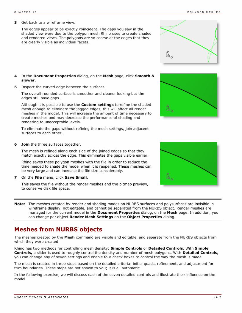
C H A P T E R 1 6 P O L Y G O N M E S H E S
Robert McNeel & Associates 160
3 Get back to a wireframe view.
The edges appear to be exactly coincident. The gaps you saw in the
shaded view were due to the polygon mesh Rhino uses to create shaded and rendered views. The polygons are so coarse at the edges that they are clearly visible as individual facets.
4 In the Document Properties dialog, on the Mesh page, click Smooth & slower.
5 Inspect the curved edge between the surfaces.
The overall rounded surface is smoother and cleaner looking but the
edges still have gaps.
Although it is possible to use the Custom settings to refine the shaded mesh enough to eliminate the jagged edges, this will affect all render meshes in the model. This will increase the amount of time necessary to create meshes and may decrease the performance of shading and rendering to unacceptable levels.
To eliminate the gaps without refining the mesh settings, join adjacent
surfaces to each other.
6 Join the three surfaces together.
The mesh is refined along each side of the joined edges so that they match exactly across the edge. This eliminates the gaps visible earlier.
Rhino saves these polygon meshes with the file in order to reduce the
time needed to shade the model when it is reopened. These meshes can be very large and can increase the file size considerably.
7 On the File menu, click Save Small.
This saves the file without the render meshes and the bitmap preview, to conserve disk file space.
Note: The meshes created by render and shading modes on NURBS surfaces and polysurfaces are invisible in wireframe display, not editable, and cannot be separated from the NURBS object. Render meshes are managed for the current model in the Document Properties dialog, on the Mesh page. In addition, you
can change per object Render Mesh Settings on the Object Properties dialog.
Meshes from NURBS objects
The meshes created by the Mesh command are visible and editable, and separate from the NURBS objects from which they were created.
Rhino has two methods for controlling mesh density: Simple Controls or Detailed Controls. With Simple Controls, a slider is used to roughly control the density and number of mesh polygons. With Detailed Controls, you can change any of seven settings and enable four check boxes to control the way the mesh is made.
The mesh is created in three steps based on the detailed criteria: initial quads, refinement, and adjustment for trim boundaries. These steps are not shown to you; it is all automatic.
In the following exercise, we will discuss each of the seven detailed controls and illustrate their influence on the model.

C H A P T E R 1 6 P O L Y G O N M E S H E S
Robert McNeel & Associates 161
Polygon Mesh Detailed Options
Density
Uses a formula to control how close the polygon edges are to the original surface. Values between 0 and 1. Larger values result in a mesh with a higher polygon count.
Maximum angle
The maximum angle between adjacent faces in the mesh. Smaller values result in slower meshing, more accurate meshes, and higher polygon count.
Maximum aspect ratio
The maximum ratio length to width of triangles in the initial grid quads.
Minimum edge length
Bigger values result in faster meshing, less accurate meshes and lower polygon count. Controls the minimum length of the sides of quads and triangles of the mesh.
Maximum edge length
Smaller values result in slower meshing and higher polygon count with more equally sized polygons. When Refine mesh is selected, polygons are refined until all polygon edges are shorter than this value. This is also approximately the maximum edge length of the quads in the initial mesh grid.
Maximum distance, edge to surface
Smaller values result in slower meshing, more accurate meshes, and higher polygon count. When Refine is selected, polygons are refined until the distance from a polygon edge midpoint to the NURBS surface is smaller than this value. This is also approximately the maximum distance from polygon edge midpoints to the NURBS surface in the initial mesh grid.
Minimum initial grid quads
Bigger values result in slower meshing, more accurate meshes, and higher polygon count with more evenly distributed polygons. This is the minimum number of quads in the mesh before any of the other refinements are applied. If you set a number for this and set all other values to 0, this will be the mesh returned.
To create a mesh using detailed controls
1 Select the object.
2 Start the Mesh command (Mesh menu: From NURBS Object).
The Polygon Mesh Options dialog appears.

C H A P T E R 1 6 P O L Y G O N M E S H E S
Robert McNeel & Associates 162
3 In the Polygon Mesh Options dialog, click Detailed Controls.
The Polygon Mesh Detailed Controls dialog appears. These settings are saved to the Windows Registry when
you exit Rhino.
4 In the Polygon Mesh Detailed Options dialog, set the following, if they are not already set: Density=0.5 Maximum angle=0.0
Maximum aspect ratio=0.0 Minimum edge length=0.0001 Maximum edge length=0.0 Maximum distance, edge to surface=0.0 Minimum initial grid quads=0 Check Refine.
Uncheck Jagged seams. Uncheck Simple planes. Check Pack Textures.
Click OK.
A mesh is created using the default settings.
5 Hide the original polysurface, change the viewport display mode to Rendered, and use the Flat Shade
display mode to view the output.
The Flat Shade display mode shows what the model would look like if it were output for prototyping or machining at this mesh density.
6 Undo the previous operation, repeat the Mesh command, and then make the following changes in the Polygon Mesh Detailed Controls dialog: Maximum angle=0.0 Maximum aspect ratio=2.0
Click OK.
Note the changes in polygon count, the shape of the mesh, and the quality of the flat-shaded mesh.
7 Undo the previous operation, repeat the Mesh command, and then make
the following changes in the Polygon Mesh Detailed Controls dialog: Minimum initial grid quads=16
Note the changes in polygon count, the shape of the mesh, and the quality of the flat-shaded mesh.
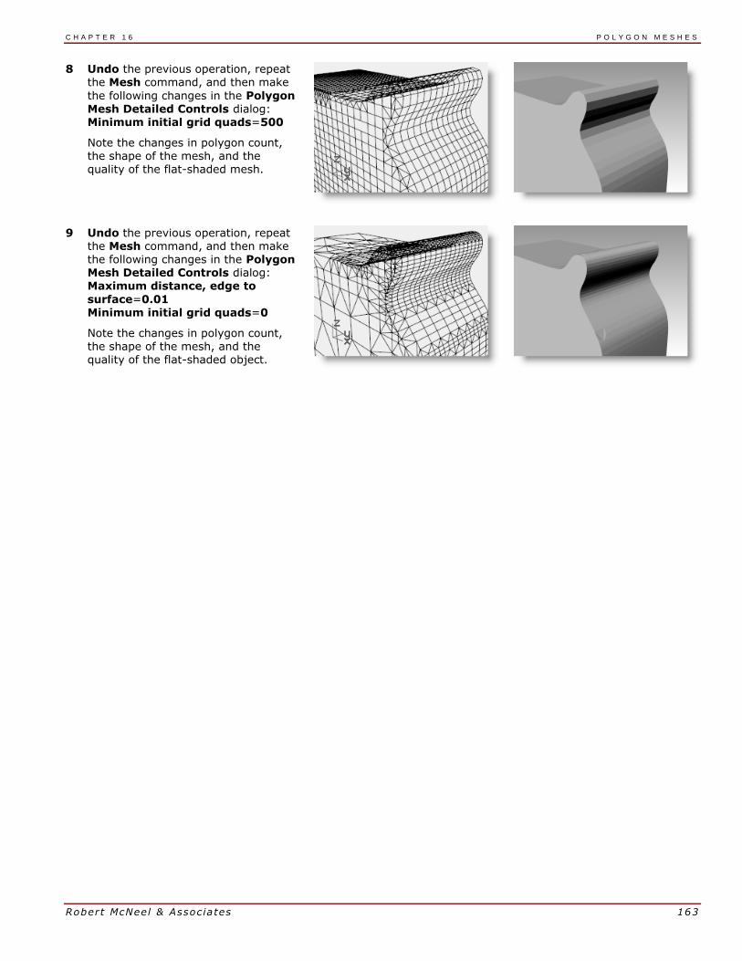
C H A P T E R 1 6 P O L Y G O N M E S H E S
Robert McNeel & Associates 163
8 Undo the previous operation, repeat the Mesh command, and then make
the following changes in the Polygon
Mesh Detailed Controls dialog: Minimum initial grid quads=500
Note the changes in polygon count, the shape of the mesh, and the quality of the flat-shaded mesh.
9 Undo the previous operation, repeat the Mesh command, and then make the following changes in the Polygon Mesh Detailed Controls dialog: Maximum distance, edge to
surface=0.01
Minimum initial grid quads=0
Note the changes in polygon count, the shape of the mesh, and the quality of the flat-shaded object.


PART IV: Rendering


Rober t McNeel & Assoc ia tes 167
17 Rendering With Rhino, creating design renderings of Rhino models is easy. Simply add materials, lights, and render.
There are several controls in the basic Rhino renderer that allows you to create some interesting special effects.
In the following exercise, we will render with and without isocurves, adjust colors, transparency, and ambient light to create images with special effects.
Exercise 36—Rhino rendering
1 Open the model Finished Detergent Bottle.3dm.
2 On the Render menu, click Current Renderer, and then click Rhino Render.
3 In the Document Properties dialog, on the Rhino Render page, scroll down to the Miscellaneous section and check Use lights on layers that are off.
4 Select the bottle and use the Properties command, on the Material page,
to assign it a Basic color of Light Gray. Set the Gloss Color to Light Blue (R=163, G=163, B=194) and the Gloss Finish to 60. Name the material Blue plastic.
5 Select the cap and use the Properties command, on the Material page, to assign it a Basic color of Tan (R=222, G=172, B=112). Set the Gloss Color to White and the Gloss Finish to 90. Name the material Tan plastic.
6 Render the Perspective viewport.
To render with isocurves displayed
1 Start the DocumentProperties command.
2 In the Document Properties dialog, on the Rhino Render page, scroll down to the Miscellaneous section and check Render surface edges and isocurves.
3 Render the Perspective viewport.
The wire color is the same as the layer color because the object's wire color is set to By Layer.

C H A P T E R 1 7 R E N D E R I N G
Robert McNeel & Associates 168
4 Use the Properties command, on the Object page, to change the Display Color to black, and then Render the Perspective viewport.
The objects are rendered with black isocurves.
To render a transparent material with isocurves displayed
1 Use the Properties command, on the Material page, to change Transparency to 70, and then Render the Perspective viewport.
The objects are rendered with black isocurves and the material is transparent.
2 Use the Properties command, on the Object page, to change the Display color to white, and then Render the Perspective viewport.
The objects are rendered with white isocurves and the material is transparent.
3 Experiment with these adjustments to get the desired effect.
4 Turn on the Lights layer and adjust the properties of the lights for more subtle changes.

C H A P T E R 1 7 R E N D E R I N G
Robert McNeel & Associates 169
Rendering properties
With Rhino’s Material Editor, you can assign any combination of color,
reflectivity, transparency, highlight, multiple bitmaps, and environments.
In the following exercise, we will add environment settings, add
materials and lights, create custom materials, edit materials, add decals to objects, and render a scene.
Exercise 37—Rendering a scene
To set up the rendering properties
The rendering properties include environment settings, render, and ambient light settings.
1 Open the model Mug.3dm.
2 From the Panels menu, click Environments and Ground Plane to open the panels we will use to set a background environment, and to add an infinite ground
plane to the scene.
This can also be accomplished by right-clicking on the Properties panel tab.
3 In the Environments panel, set the background to Environment and click [+] to add an environment.
4 In the Open dialog, double-click Environments, click Rhino Interior.renv, and then click Open.

C H A P T E R 1 7 R E N D E R I N G
Robert McNeel & Associates 170
5 In the Ground Plane panel, check On for Ground plane options.
The ground plane will automatically be set for the default material.
6 Render the Perspective viewport.
To assign materials to layers
1 In the Layers panel, select the Floss Blister layer, and click in its Material column.
2 From the Layer Material dialog, choose Thin Clear Plastic from the dropdown list, and click OK.
3 In the Layers panel, select the Floss Container and Toothpaste Tube layers, and click in the Material column got one of them.
4 From the Layer Material dialog, choose White Shiny from the dropdown list, and click OK.

C H A P T E R 1 7 R E N D E R I N G
Robert McNeel & Associates 171
Scene lighting
So far, we have used the default lighting in Rhino. This invisible light comes from over the viewer’s left shoulder.
It is enough to illuminate the model and to give you a starting point. The default light is on only if no other lights are on in the scene and it cannot be modified. In order to control the lighting, we are going to add our own lights.
To add lights
1 From the Render menu, click Create Spotlight.
2 Make a large spotlight that shines on the scene from the front and slightly above as shown on the right.
Use elevator mode, or turn on the
spotlight’s control points and drag them to move the light into position.
Spotlight, front view
Spotlight, right view
Spotlight, perspective view
3 Adjust the Properties of the light as shown: Shadow intensity=40 Spotlight hardness=50 Light intensity=50

C H A P T E R 1 7 R E N D E R I N G
Robert McNeel & Associates 172
4 Render the Perspective viewport.
This makes a nicer image, but two or three lights in a scene
improve the rendering. We are going to add another light to create highlights on the mug.
To add a second light
1 Select the first light.
2 In the Top viewport, Mirror the light across the vertical axis.
3 Adjust the Properties of the light as shown: Shadow intensity=60 Spotlight hardness=30 Light intensity=40
Spotlight, front view
4 Render the Perspective viewport.
To add a third light
1 From the Render menu, click Create Spotlight.
2 Make a large spotlight that shines on the scene from the below.
This light will be used to add a little light to the underside of the toothpaste tube and the floss packet.
3 Adjust the Properties of the light as shown: Shadow intensity=0 Spotlight hardness=25
Light intensity=20
Spotlight, front view

C H A P T E R 1 7 R E N D E R I N G
Robert McNeel & Associates 173
5 Render the Perspective viewport.
It is important to turn the shadow intensity to 0 so that the light will
penetrate through the ground plane.
To make a material from scratch and assign it to a layer
1 Open the Layers dialog.
2 In the Layers dialog, select the Mug layer, and click in the Material
column.
3 In the Layer Material dialog, click More Types.
4 In the Types dialog, click on Basic Material and then click OK.
5 Name the material Green Ceramic.
Set the following: Color to Green (R=21, G=210, B=180)
Gloss finish to 90 Gloss color to (R=198, G=247, B=255) Reflectivity to 30 Reflectivity color to (R=21, G=225, B=180)
6 Render the Perspective viewport.
Image and bump maps
Instead of simply using color for your material, you can use an image of a material. You can scan photographs and real objects like wallpaper and carpet, create patterns in a paint program, or use images from libraries of textures from other renderers, or other sources of bitmap images.
Image mapping uses bitmap images to add detail to the material. You can use images to alter many attributes of the material’s surface including its color pattern and apparent three-dimensional surface quality (bump). Procedural bumps add a random roughness or knurled quality to the surface.

C H A P T E R 1 7 R E N D E R I N G
Robert McNeel & Associates 174
To create a new material from an existing material
1 In the Materials panel, right-click White shiny, and then
click, Duplicate.
2 Name the duplicated material Toothpaste Cap.
3 In the Textures section, under Color, click (empty – click to assign).
4 In the Open dialog, double-click on Tube Bump.png.
5 In the Textures section, click on Tube Bump to see additional settings.
6 In the Mapping section, set the U Repeat to 8.
7 Assign the new material to the Toothpaste Cap layer or
assign it to the object. Adjust the mapping as necessary.
8 Render the Perspective viewport.
The cap has a grooved appearance. The repeat number determines how close together the grooves appear.
Decals
A decal is the method Rhino uses to apply an image bitmap to a specific area of an object.
The decal mapping type tells Rhino how to project the decal onto your object. The four mapping types, planar,
cylindrical, spherical, and UV, are described below.
Decal options
Planar
The planar mapping type is the most common mapping type. It is appropriate when mapping to flat or gently
curved objects.
Cylindrical
The cylindrical mapping type is useful for placing decals onto objects that curve in one direction, such as labels on wine bottles.
The cylindrical projection maps the bitmap onto the mapping cylinder with the bitmap’s vertical axis along the cylinder’s axis, and the horizontal axis around the cylinder, like a wine bottle label.
Spherical
The spherical mapping type is useful for placing images onto objects that curve in two directions. The spherical projection maps the bitmap onto the mapping sphere with the bitmap’s vertical axis (height), curving from pole to pole, and the horizontal axis curving around the equator.
Initially the mapping sphere’s equator is assumed to be parallel to the current construction plane, and the sphere’s axis is parallel to the construction plane z-axis. Later you can modify its orientation.
UV
UV mapping stretches the image to fit the whole surface. The U- and V-directions of the surface determine which direction the map is applied. There are no controls.
UV mapping works well for organic shapes, hair, skin, and plant structures.
On trimmed surfaces and polysurfaces, only parts of the image may appear in the rendering. UV mapping stretches the bitmap over the whole UV range of the surface. If some of that range has been trimmed away,
the corresponding parts of the bitmap will not be visible.

C H A P T E R 1 7 R E N D E R I N G
Robert McNeel & Associates 175
To map a decal with planar projection
1 Turn on the Decal reference planes
layer.
2 Select the toothpaste box.
3 In the Properties panel, on the Decals page, click Add
4 Select the Minty Green-Box Upper.jpg.
5 Click Open.
6 Click Planar and then OK.
7 Using object snaps, pick locations for the decal Location (1), the Width (2), and Height (3) direction of the decal.
These three points define the decal plane’s location and extents. The decal plane must lie on or behind the surface of the object. The decal
projects up from the decal plane. Portions of the surface that lie behind the decal plane will not show the decal.
After the decal is placed, you can click the control points on the decal control wireframe to move, rotate, or stretch the decal.
8 Press Enter or right-click to set the location.
Place more decals
1 Continue to place bitmaps on the sides, flaps, and ends of the box.
2 Use planar mapping to put the decals on the floss container and the toothpaste tube.
The magenta rectangles were created to assist with placement of the decals.
3 Render the Perspective viewport.
To map a decal with cylindrical projection
The circle of the mapping cylinder is initially parallel to the current construction plane, and the cylinder’s axis is parallel to the construction plane z-axis.
1 Select the mug.
2 Start the Properties command (Edit menu: Object Properties).
3 In the Properties panel, on the Decals page, click Add.
4 Select the Sailboat-002.tif.
5 In the Decal Mapping Style dialog, click Cylindrical.

C H A P T E R 1 7 R E N D E R I N G
Robert McNeel & Associates 176
6 Use the magenta circle for the Center of cylinder and a Radius or Diameter for the decal.
The controls then let you click the control points on the decal control wireframe to move, rotate, or stretch the decal cylinder.
7 Press Enter or right-click to set the location.
8 Render the Perspective viewport.
9 Turn on the toothbrush layers.
10 Adjust the materials settings and lighting as needed to get the desired results.