rheology and performance evaluation of polyoctenamer as asphalt rubber modifier in hot mix

Graduate Theses and Dissertations Iowa State University Capstones, Theses andDissertations

2013

Rheology and performance evaluation ofPolyoctenamer as Asphalt Rubber modifier in HotMix AsphaltKa Lai Nieve Ng PugaIowa State University

Follow this and additional works at: https://lib.dr.iastate.edu/etd

Part of the Civil Engineering Commons

This Thesis is brought to you for free and open access by the Iowa State University Capstones, Theses and Dissertations at Iowa State University DigitalRepository. It has been accepted for inclusion in Graduate Theses and Dissertations by an authorized administrator of Iowa State University DigitalRepository. For more information, please contact [email protected].

Recommended CitationNg Puga, Ka Lai Nieve, "Rheology and performance evaluation of Polyoctenamer as Asphalt Rubber modifier in Hot Mix Asphalt"(2013). Graduate Theses and Dissertations. 13279.https://lib.dr.iastate.edu/etd/13279

http://lib.dr.iastate.edu/?utm_source=lib.dr.iastate.edu%2Fetd%2F13279&utm_medium=PDF&utm_campaign=PDFCoverPages

http://lib.dr.iastate.edu/?utm_source=lib.dr.iastate.edu%2Fetd%2F13279&utm_medium=PDF&utm_campaign=PDFCoverPages

https://lib.dr.iastate.edu/etd?utm_source=lib.dr.iastate.edu%2Fetd%2F13279&utm_medium=PDF&utm_campaign=PDFCoverPages

https://lib.dr.iastate.edu/theses?utm_source=lib.dr.iastate.edu%2Fetd%2F13279&utm_medium=PDF&utm_campaign=PDFCoverPages

https://lib.dr.iastate.edu/theses?utm_source=lib.dr.iastate.edu%2Fetd%2F13279&utm_medium=PDF&utm_campaign=PDFCoverPages

https://lib.dr.iastate.edu/etd?utm_source=lib.dr.iastate.edu%2Fetd%2F13279&utm_medium=PDF&utm_campaign=PDFCoverPages

http://network.bepress.com/hgg/discipline/252?utm_source=lib.dr.iastate.edu%2Fetd%2F13279&utm_medium=PDF&utm_campaign=PDFCoverPages

https://lib.dr.iastate.edu/etd/13279?utm_source=lib.dr.iastate.edu%2Fetd%2F13279&utm_medium=PDF&utm_campaign=PDFCoverPages

mailto:[email protected]

Rheology and performance evaluation of Polyoctenamer

as Asphalt Rubber modifier in Hot Mix Asphalt

by

Ka Lai Nieve Ng Puga

A thesis submitted to the graduate faculty

in partial fulfillment of the requirements for the degree of

MASTER OF SCIENCE

Major: Civil Engineering (Civil Engineering Materials)

Program of Study Committee:

R. Christopher Williams, Major Professor

Vernon R. Schaefer

W. Robert Stephenson

Iowa State University

Ames, Iowa

2013

Copyright © Ka Lai Nieve Ng Puga, 2013. All rights reserved.

ii

TABLE OF CONTENTS

LIST OF TABLES ............................................................................................................. iv

LIST OF FIGURES ........................................................................................................... vi

ACKNOWLEDGEMENTS ............................................................................................. viii

ABSTRACT ....................................................................................................................... ix

CHAPTER 1. INTRODUCTION ...................................................................................... 1

Background ............................................................................................................. 1

Problem Statement .................................................................................................. 1

Objectives ............................................................................................................... 2

Methodology ........................................................................................................... 2

Hypothesis............................................................................................................... 3

Organization ............................................................................................................ 3

CHAPTER 2. LITERATURE REVIEW ........................................................................... 5

Asphalt cement........................................................................................................ 5

Ground Tire Rubber ................................................................................................ 7

Asphalt rubber mixtures and asphalt rubber binders ............................................ 12

Use of asphalt rubber in the United States ............................................... 14

Production of asphalt rubber mixtures and binders ................................. 17

Polyoctenamer (PO) .............................................................................................. 24

CHAPTER 3. EXPERIMENTAL PLAN AND TESTING METHODS......................... 28

Binders .................................................................................................................. 28

Density testing ........................................................................................... 29

Viscosity testing ........................................................................................ 31

Dynamic Shear Rheometer (DSR) ............................................................ 32

Mass Loss .................................................................................................. 35

Bending Beam Rheometer (BBR) .............................................................. 36

Binders Master Curves ............................................................................. 37

Mixtures ................................................................................................................ 39

Dynamic Modulus (E*) test ...................................................................... 42

Mixtures Master Curves ............................................................................ 44

Flow Number test ...................................................................................... 44

Tensile Strength Ratio ............................................................................... 45

CHAPTER 4. RESULTS AND DISCUSSION ............................................................... 47

Binders Testing Results ........................................................................................ 47

Densities .................................................................................................... 47

Viscosity .................................................................................................... 48

Dynamic Shear Rheometer (DSR) ............................................................ 56

Mass Loss .................................................................................................. 60

iii

Bending Beam Rheometer (BBR) .............................................................. 61

Asphalt Binders Master Curves ................................................................ 63

Mixes Performance Testing Results ..................................................................... 68

Dynamic Modulus (E*) ............................................................................. 68

Asphalt Rubber Mixtures Master Curves .................................................. 68

Flow Number (FN) .................................................................................... 73

Tensile Strength Ratio (TSR) .................................................................... 75

CHAPTER 5. CONCLUSIONS AND RECOMMENDATIONS ................................... 79

Binders .................................................................................................................. 79

Mixes..................................................................................................................... 81

REFERENCES ................................................................................................................. 83

APPENDIX A. DYNAMIC MODULUS TEST RESULTS ........................................... 89

APPENDIX B. FLOW NUMBER TEST RESULTS ...................................................... 97

APPENDIX C. TENSILE STRENGTH RATIO RESULTS .......................................... 98

iv

LIST OF TABLES

Table 1. Typical weight distribution of the various components of a tire ......................... 8

Table 2. Matrix of binders developed .............................................................................. 28

Table 3. Testing experimental plan for binder properties ................................................ 29

Table 4. Parameters used for frequency sweeps .............................................................. 37

Table 5. Aggregates Gradation ........................................................................................ 40

Table 6. Testing experimental plan for mixes performance ............................................ 42

Table 7. Asphalt rubber binders densities ........................................................................ 47

Table 8. Average viscosity of the asphalt rubber binders ................................................ 48

Table 9. Binder viscosities ANOVA table ....................................................................... 53

Table 10. Binder viscosity least square means differences due to binder type ............... 53

Table 11. Binder viscosities least square means due to testing temperature ................... 54

Table 12. Binder viscosities least square means due to testing rotational speed ............. 55

Table 13. High temperature continuous grading of binders ............................................ 57

Table 14. Intermediate temperature continuous grading of PAV aged binders ............... 59

Table 15. Summary of average percentage mass loss ..................................................... 60

Table 16. Low Temperature continuous grading of binders ............................................ 62

Table 17. Dynamic modulus ANOVA table .................................................................... 73

Table 18. Flow number ANOVA table ............................................................................ 74

Table 19. Flow number least square means differences .................................................. 75

Table 20. Tensile strength ratio ANOVA table ............................................................... 76

Table 21. Peak load ANOVA table ................................................................................. 77

Table A. 1. Dynamic modulus test results, E* AMB ...................................................... 89

Table A. 2. Dynamic modulus test results, E* AV .......................................................... 90

v

Table A. 3. Dynamic modulus test results, E* CRYO .................................................... 91

Table A. 4. Dynamic modulus test results, E* CV .......................................................... 92

Table A. 5. Dynamic modulus test results, φ AMB ......................................................... 93

Table A. 6. Dynamic modulus test results, φ AV ............................................................ 94

Table A. 7. Dynamic modulus test results, φ CRYO ....................................................... 95

Table A. 8. Dynamic modulus test results, φ CV ............................................................ 96

Table B. 1. Summary of flow number test results ........................................................... 97

Table C. 1. Tensile Strength Ratio (TSR) results ............................................................ 98

vi

LIST OF FIGURES

Figure 1. Chemical fractions of Asphalt (SARA fractions) (Lesueur, 2009) .................... 6

Figure 2. Cross section of a high-performance tire (Mark, 2005) ..................................... 8

Figure 3. Types of GTR (a) Ambient GTR (b) Cryogenic GTR ..................................... 10

Figure 4. Ambient scrap tire processing plant schematics (Reschner, 2006) .................. 11

Figure 5. Cryogenic scrap tire processing plant schematics (Reschner, 2006) ............... 12

Figure 6. Different asphalt rubber applications ............................................................... 13

Figure 7. Depiction of reaction stages of asphalt and rubber .......................................... 19

Figure 8. Example of on-site asphalt rubber blending plant ............................................ 21

Figure 9. Example of asphalt rubber reaction tank .......................................................... 22

Figure 10. Depiction of auger system inside a horizontal blending tank ........................ 22

Figure 11. Special asphalt rubber pump with special heat tracing and relief valve ........ 23

Figure 12. Synthesis of trans-polyoctenamer .................................................................. 25

Figure 13. Polyoctenamer pellets 80% crystalline ........................................................... 26

Figure 14. TA dynamic shear rheometer ......................................................................... 32

Figure 15. Rolling thin film oven .................................................................................... 34

Figure 16. Pressurized aging vessel ................................................................................. 35

Figure 17. Vacuum oven .................................................................................................. 35

Figure 18. Bending beam rheometer ................................................................................ 36

Figure 19. 0.45 power chart for 19.0 mm NMAS particle size distribution .................... 40

Figure 20. Universal testing machine (UTM-25) and data acquisition system ............... 43

Figure 21. Dynamic modulus testing setup ..................................................................... 43

Figure 22. Flow number sample before and after testing ................................................ 45

Figure 23. Two hour moisture conditioning .................................................................... 46

Figure 24. Indirect tensile strength test setup .................................................................. 46

vii

Figure 25. Average viscosities of AMB binder ............................................................... 50

Figure 26. Average viscosities of AV binder .................................................................. 50

Figure 27. Average viscosities of CRYO binder ............................................................. 51

Figure 28. Average viscosities of CV binder ................................................................... 51

Figure 29. Comparison of viscosities at a testing rotational speed of 20rpm .................. 52

Figure 30. Binder type least square means plot ............................................................... 54

Figure 31. Testing temperature least square means plot .................................................. 55

Figure 32. Testing speed least square means plot ............................................................ 55

Figure 33. Binder type * speed least square means plot .................................................. 56

Figure 34. High temperature continuous grading ............................................................ 58

Figure 35. Intermediate temperature continuous grading for PAV Aged binders ........... 60

Figure 36. Average percentage mass loss ........................................................................ 61

Figure 37. BBR low temperature continuous grading ..................................................... 63

Figure 38. Master curves of Unaged asphalt rubber binders ........................................... 65

Figure 39. Master curves of RTFO asphalt rubber binders ............................................. 66

Figure 40. Master curves of PAV Aged asphalt rubber binders ...................................... 67

Figure 41. Master curve of AMB Mix ............................................................................. 70

Figure 42. Master curve of AV Mix ................................................................................ 71

Figure 43. Master curve of CRYO Mix ........................................................................... 71

Figure 44. Master curve of CV Mix ................................................................................ 72

Figure 45. Comparison between master curves mixtures ................................................ 72

Figure 46. Average Flow Number ................................................................................... 74

Figure 47. Average Tensile Strength Ratios .................................................................... 76

Figure 48. Treatment least square means plot for peak load ........................................... 78

Figure 49. Indirect tensile strength specimens tested ...................................................... 78

viii

ACKNOWLEDGEMENTS

First, I would like to thank God for always blessing me in so many ways, and for

allowing me to reach one of my dearest goals. Second, I would like to thank my family

for all the support that they have given me, my mom, dad and specially my sisters for

always cheering me up in the moments I need it the most.

I also want to thank Dr. Williams, for allowing me to work with him, for always

mentoring and teaching me through my graduate studies. In addition, I would like to give

special thanks to Dr. Schaefer and Dr. Stephenson for not only being part of my POS

committee but for being such great professors, with them I not only learned a great deal

of things, but I enjoyed every class.

I want to give thanks to my laboratory graduate colleagues, Andy Cascione,

Ashley Buss, Oscar Echavarria and Jianhua Yu for the help they provided me throughout

this research. At least but not last, special thanks to my dearest friend and colleague

Joana Peralta, who not only helped me a great deal but provided me with very helpful

insights on this research.

ix

ABSTRACT

The high amount of scrap tires that are generated annually in the United States are

stored in stockpiles, landfills and dumps all over the United States. Tires are mostly

composed of rubber; and they can be recycled to obtain two types of ground tire rubber

(GTR), ambient and cryogenic. Tire recycling can help reduce the accumulations of

scrap tires, while the GTR can be used in many applications in different industries.

The asphalt industry has used GTR in highway pavement construction since the

1960’s. GTR can be blended with any conventional asphalt binder to produce asphalt

rubber binders, that due to the elastomeric properties of the GTR, will have better

performance at high and intermediate temperatures than conventional binders. However,

one of the challenges of asphalt rubber technology is its high viscosity, which increases

its mixing and compaction temperatures when compared to conventional asphalts.

The objective of this research is to characterize the effects of the binder additive

polyoctenamer (PO) on the rheological properties of laboratory-produced asphalt rubber

binders with a base asphalt of PG46-34 and two different types of ground tire rubber

(ambient and cryogenic); also, to see the effects of PO in the characterization of the

performance of asphalt rubber mixtures.

The laboratory-produced binders were evaluated following the Superpave binder

specification and testing procedures. Densities, viscosities, complex modulus (G*), mass

losses, creep stiffness were obtained from the binders. The statistical analysis performed

on the binders demonstrated that the addition of PO improves the viscosities of asphalt

rubber thereby obtaining a reduction in the estimated mixing and compaction

temperatures. The binder grading demonstrates that PO does not affect negatively the

x

final performance grading for high, intermediate and low temperature. Further, the

construction of the master curves showed that asphalt rubber binders with and without

PO have similar stiffness performance.

The performances for the dynamic modulus, flow number and indirect tensile

strength ratio test of the laboratory-produced mixtures with and without PO were not

statistically different. Accordingly, the mixes’ master curves showed no difference.

Overall, the addition of PO does not negatively affect the performance of asphalt rubber

mixes.

1

CHAPTER 1. INTRODUCTION

Background

The use of asphalt rubber binders to produce asphalt rubber mixtures is very

common in geographic areas where rutting performance is a problem. In general, one of

the difficulties of applying asphalt rubber technology is the high temperatures required

for mixing and compaction of the mentioned mixtures when compared with conventional

asphalt mixtures, due to the high viscosities encountered in asphalt rubber binders. The

high temperatures used to produce the asphalt rubber binders and mixes carries an

associated energy cost.

Therefore, the addition of chemical modifiers to asphalt rubber binders is used to

improve the rheological properties of these binders to help reduce the mixing and

compaction temperatures of their mixes and in turn reduce the energy cost of producing

these asphalt rubber mixes. However, whenever a modification of binders is made, a

comprehensive study on the real effects of the modifiers on the binder’s rheological

performance and on the mixes’ performance is needed.

Problem Statement

Asphalt rubber binder is known for having higher viscosities when compared to

conventional asphalt binders at a certain temperature. This causes the increase in mixing

and compacting temperatures of asphalt mixtures to obtain the desirable viscosity

required by the standard specifications to perform these activities.

It is believed that the addition of a binder additive like polyoctenamer (PO) will

help reduce the viscosity of asphalt rubber binder without negatively affecting its

2

rheological properties. Likewise, it is thought that PO will not affect the performance of

the asphalt rubber mixtures, but it will help decrease the mixing and compacting

temperatures generally used in the asphalt rubber technology.

Objectives

The objectives of this study are to determine if PO affects the rheological

properties of asphalt rubber binders produced with a base asphalt of PG46-34 and two

different types of ground tire rubber (ambient GTR and cryogenic GTR). Also it will be

determined if the performance of the asphalt rubber mixtures are influenced by the

addition of PO.

Methodology

The experimental plan carried out in this study uses four laboratory-produced

asphalt rubber binders following the procedure described in Chapter 3, and four

laboratory-produced asphalt rubber mixes with the mentioned binders following the

SuperPave mix design procedure.

The laboratory-produced binders were tested following the SuperPave

performance graded asphalt binder specifications and testing procedures. Some of the

tests performed to characterize the binders are density by means of a pycnometer test;

dynamic shear rheometer tests on unaged, rolling thin film oven (RTFO) aged and

pressurized aging vessel (PAV) aged materials to determine the performance grade; mass

loss determination on the RTFO aged materials; and bending beam rheometer tests on the

PAV aged materials. From the results of the dynamic shear rheometer, master curves for

unaged, RTFO and PAV aged materials were constructed.

3

The performance of the laboratory-produced asphalt rubber mixes were then

tested for their stiffness performance through the dynamic modulus testing, their rutting

characterization by means of the flow number test and their moisture-susceptibility

evaluated using the tensile strength ratio test. Master curves from the results of the

dynamic modulus test were built for the four types of asphalt rubber mixtures.

Hypothesis

The following are the hypothesis used to evaluate statistically the results of the

experimental plan presented in Chapter 3.

The addition of PO to asphalt rubber binders influences the viscosity of the binders.

The addition of PO to asphalt rubber binders reduces the compaction and mixing

temperatures of their mixes

The addition of PO to asphalt rubber mixes affects the high temperature performance

of the mixes.

The addition of PO to asphalt rubber mixes impacts the intermediate temperature

performance of the mixes.

The addition of PO influences to asphalt rubber mixes the low temperature

performance of the mixes

The addition of PO affects the rutting performance of asphalt rubber mixes.

The addition of PO has an effect in the tensile strength ratio of asphalt rubber mixes

Organization

This thesis is divided in five chapters, including this Chapter 1 which provides a

background on Asphalt Rubber, the problem statement, objectives, methodology and

hypotheses in this study. Chapter 2 presents a literature review on Asphalt Rubber and

PO. Chapter 3 describes the experimental plan and the properties of the materials, as

well as the testing procedures followed to perform the characterization of the asphalt

4

rubber binders and mixtures developed. In Chapter 4 the results obtained for each testing

are presented; and statistical analyses are performed and discussed accordingly. Finally,

Chapter 5 presents a summary of the findings, conclusions and recommendations for

further investigation on this topic.

5

CHAPTER 2. LITERATURE REVIEW

Asphalt cement

Asphalt is considered a bituminous material. It is a dark brown to black

cementitious material that can be found naturally or it can be produced through petroleum

(crude oils) distillation. The main producers of asphalt from crude oils in the world are

countries like Mexico, Venezuela, Canada and the Middle East. In the United States, the

main crude oil sources come from the Gulf Coast, Southwest, Rocky Mountain, West

Coast regions and the North side of Alaska (Roberts, 2009).

The distillation process of the crude petroleum consists in the separation of the

crude into various fractions that have different boiling ranges. The petroleum is heated in

a large furnace at temperatures about 650°F (343°C) and vaporized. The vapors are then

condensed in a distillation column where the lightest components rise and are cooled and

extracted as gasoline, naphtha, kerosene and light gas oil. The heavier fractions or

residues of this distillation are fed to a vacuum distillation unit and heavier gas oils are

obtained. The residue of this vacuum distillation is then known as steam refined asphalt

cement (Roberts, 2009).

The chemical composition of distilled asphalt consists of different fractions,

known as SARA fractions. SARA stands for saturates, aromatics, resins and asphaltenes.

The saturates of the asphalt represent around 5-15 weight percentage of the total amount

of the asphalt. The aromatics part, also known as naphtene aromatics, constitute together

with the asphaltenes most of the asphalt with around 30-45 weight percentage of the

asphalt. Resins are polar aromatics that can make up to 30-45 by weight percentage of

the asphalt, whereas the asphaltenes constitutes between 5 and 20 percent of asphalt.

6

Asphaltenes are known to be the insoluble part of asphalt in n-heptane, meanwhile

saturates, aromatics and resins are grouped together into Maltenes, and they represent the

soluble part of asphalt in n-heptane. Figure 1 presents a graphical depiction of the SARA

fractions in asphalt (Lesueur, 2009).

Figure 1. Chemical fractions of Asphalt (SARA fractions) (Lesueur, 2009)

Depending on the source of the crude-oil petroleum and the distillation process

techniques applied, the composition of the asphalt cement will vary, thus its intrinsic

properties will be different. The asphalt composition will affect its softening point,

viscosity, shear susceptibility and complex (stress-strain) modulus. The asphaltene

content will influence the softening point of the asphalt in a linear fashion; this means

that the softening point will increase as asphaltenes increase (Oyekunle, 2007).

Meanwhile, saturates and naphtene-aromatics have low softening points compared to

polar-aromatics and asphaltenes which have high softening points (Corbett, 1970).

Various methods have been developed to characterize the properties of asphalt

cements, the preferred method to characterize the asphalt cements today in the United

Asphalt

Asphaltenes

(n-heptane insoluble)

Asphaltenes

(toluene soluble)

Carbenes/Carboids

(toluene insoluble)

Carbenes

(CS2 soluble)

Carboids

(CS2 insoluble)

Maltenes

(n-heptane soluble)

Saturates

(n-heptane wash through alumina)

Aromatics

(toluene wash through alumina)

Resins

(pyridine wash through alumina)

7

States is the performance based grade method developed by the Strategic Highway

Research Program (SHRP) from 1987-1992 and better known as Superpave binder

specifications.

The asphalt cement properties are characterized through the performance of the

asphalt at high, intermediate and low temperatures under the Superpave binder

specifications. The performance at high temperatures are related to the rutting resistance

of the asphalt cement, the performance at intermediate temperatures are more related to

fatigue cracking and the low temperatures performance to thermal cracking. The

performance grade designation consists of a “PGXX-ZZ” designation, where “PG” stands

for performance grade, “XX” is a number that corresponds to the high temperature

performance grade and “ZZ” is the number related to the minimum low temperature

grade.

Ground Tire Rubber

The generation of scrap tires in the US in 2009 was estimated to be more than 300

million tires, which represents approximately one tire per person (Rubber Manufacturers

Association, 2009). Iowans generate around 3 million scrap tires annually according to

the Iowa Department of Natural Resources website in 2013.

Modern tires are made up of many different components (Figure 2). The main

components of tires are “vulcanized rubber, rubber filler, rubberized fabric, steel cord,

fillers like carbon black or silica gel, sulfur, zinc oxide, processing oil, fabric belts, steel

wire, reinforced rubber beads and many other additives”. Table 1 presents the typical

8

weight distribution of the components of a tire and it shows that tires are mostly

composed of rubbers (Unapumnuk, 2006).

Figure 2. Cross section of a high-performance tire (Mark, 2005)

Table 1. Typical weight distribution of the various components of a tire

Tire components Percentage

Natural rubber 15-19

Carbon black 24-28

Synthetic rubber 25-29

Steel cords 9-13

Textiles cords 9-13

Chemical additives 14-15

From Unapumnuk, (2005)

9

Rubber is a type of elastomer, and as any elastomer it can go under large elastic

deformations and return to its original shape. The ASTM D 6814 (2002) defines rubber

as a natural or synthetic elastomer that can be chemically cross-linked/vulcanized to

enhance its useful properties. Cross-linked rubber forms a strong three-dimensional

chemical network. Rubber will swell in the presence of a solvent, but it will not dissolve

and cannot be reprocessed by simply heating it (Hamed, 1992).

The amount of rubber that composes scrap tires makes them a potential source of

raw material for the rubber industry. Moreover, landfills and legislation are requiring

more economical and environmental friendly ways to dispose of scrap tires. There are

many technologies to recover the rubber from scrap tires. Some of the methods that these

technologies apply include retreading, reclaiming, grinding, pulverization, microwave

and ultrasonic processes, pyrolysis, and incineration. The recycled rubber is generally

known as ground tire rubber (GTR) (Isayev, 2005).

Two types of ground tire rubber can be obtained from scrap tire recycling. These

are ambient ground tire rubber (ambGTR) and cryogenic ground tire rubber (cryoGTR).

The processes from where these are obtained are different. Figure 3 shows the two types

of ground tire rubbers that can be obtained from processing scrap tires.

Ambient GTR is obtained by the grinding of the ground tire rubber at or above

ambient temperature, without the use of any cooling system to make the rubber brittle,

through either cracker mills or a granulator. If the ambient GTR is ground using the

granulator process, the rubber particles will tend to have a cut surface shape and rough

texture. Meanwhile, if the ambient GTR is ground using cracker mills, its particles will

10

be long and narrow in shape with a high surface area (Recycling Research Institute,

2006).

Figure 3. Types of GTR (a) Ambient GTR (b) Cryogenic GTR

Figure 4 shows the schematic of an ambient rubber processing plant, where the

tires are fed into a shredder, which will reduce the tire into two inches size chips. Then

the chips go into a granulator that makes them smaller than 3 /8 inches, at this stage most

of the steel and fiber that compose the tire are freed. The steel is then removed through

magnets and the fiber is shaken out or wind sifted. When the rubber is cleaner, it goes

through finer grinding processes depending on the size desired, most of the mesh sizes

range from 10 to 30. The usual equipment used to perform this fine grinding are:

secondary granulators, high speed rotary mills, extruders or screw presses and cracker

mills (Reshner, 2006).

Whereas, cryogenic GTR is obtained through a process where the scrap tire

rubber is frozen using liquid nitrogen or other frozen method to a temperature below the

glass transition temperature of the rubber to make it brittle like glass, and then the rubber

is put in a hammermill and reduced to the desired particle size (Reschner, 2006).

11

Figure 4. Ambient scrap tire processing plant schematics (Reschner, 2006)

Figure 5 represents the schematics of a cryogenic scrap tire processing plant, in

which the tires are first fed to a shredder, like the first shredder found for the ambient

scrap tire processing plant, reducing the tire rubber to two inch sized chips. These chips

are then cooled to very low temperatures, approximately -120°C through a funnel system

that has freezing elements like nitrogen. After being frozen, the rubber is then shattered

with a hammermill system, then the steel and fibers are removed through magnets,

aspiration and screening. Next, the rubber is dried and sieved into different particles

sizes. The rubber particles obtained from the cryogenic method are even in size and

smooth, with a low surface area. (Reschner, 2006).

12

Figure 5. Cryogenic scrap tire processing plant schematics (Reschner, 2006)

Ground tire rubbers are usually used as an asphalt binder modifier due to its

elastomeric properties which improves the performance of asphalt mixtures and at the

same time it contributes to the reduction of the accumulation of scrap tires in landfills.

Asphalt rubber mixtures and asphalt rubber binders

Asphalt rubber started to be used as a binder in chip seal and dense and open

graded asphalt concrete construction. The asphalt-rubber chip seal, or seal coat, is known

as “asphalt-rubber interlayer”, which is placed beneath an asphalt concrete overlay, and it

is intended to reduced reflection cracking in overlays. The hot-mix asphalt concrete

made with asphalt-rubber binder is known by “asphalt-rubber concrete” in dense-graded

mixes and “asphalt-rubber friction course” in open-graded mixes. (Shuler, 1986)

13

The early applications of asphalt rubber can be categorized as asphalt rubber

concrete (ARC), open graded friction courses, stress absorbing membranes (SAM’s),

stress absorbing membrane interlayers (SAMI’s), cape seals, three layer systems and

waterproof membranes (FHWA, 2008). Figure 6 illustrates some cross-sections of the

aforementioned applications of asphalt rubber technology.

Figure 6. Different asphalt rubber applications

(Adopted from ARTS)

Asphalt rubber mixtures are highly resistant to oxidation and cracking due to the

presence of the antioxidants of the carbon black in the rubber, high viscosities of asphalt

rubber binders help in the rutting resistance of the mixture, while the elastic properties of

rubber help to the resistance to reflective and thermal cracking of the pavement.

14

The production of asphalt rubber mixtures can be made through two processes.

These are the wet process and the dry process. In the first process the crumb rubber is

blended into the asphalt binder prior to the production of the mixes, whereas, in the

second process the rubber is added to the aggregates before mixing it with the asphalt

binder.

Use of asphalt rubber in the United States

Charles H. McDonald developed the wet process method in the mid-1960’s. He

developed commercial binder systems in conjunction with Atlos Rubber, Arizona

Deparment of Transportation (Arizona DOT), and Sahuaro Petroleum and Asphalt

Company. By mid-1970’s, Arizona Refining Company (ARCO) also developed an

asphalt rubber system. (Caltrans, 2002)

Arizona DOT carried several comprehensive researches on asphalt rubber

between the mid-1970’s and early 1980’s, where they established that the rubber type,

rubber gradations, rubber concentration, asphalt type, asphalt concentration, extender

oils, reaction times and temperatures influenced the properties of the asphalt rubber

binders (Caltrans, 2002). The common use of asphalt rubber binder during those years

was as chip seals. However, by the beginning of 1990’s one-inch thick asphalt-rubber

mix overlays were preferred over the chip seals because the overlays provided smoother

riding surface and produced less traffic noise. Both, the chip seals and the asphalt-rubber

overlays provided retardation on the reflection of fatigue cracking and thermal cracking.

California Department of Transportation (CalTrans) started evaluating asphalt

rubber as spray applications (chip seals, interlayers and cape seals) in 1970’s and as hot

15

mix asphalt (dense-graded, open-graded, and gap-graded) in 1980’s using the wet-

process. CalTrans has reported that the use of asphalt rubber mixtures usually exhibits

less distress, requires less maintenance and handles more deflections than regular dense-

graded asphalt concrete and at least forty cities in California have asphalt rubber

pavements (Caltrans, 2002).

Texas Department of Transportation (Texas DOT) also started using asphalt

rubber in these applications around the same years as Caltrans. The most used

application in Texas for asphalt rubber is in chip seals, since after many years of use of

the technology they have concluded that asphalt rubber chip seals improve the resistance

to fatigue cracking and raveling and at the same time the cost of placing if almost have of

the cost of repaving (Estakhri et al, 1992). Dense-graded asphalt rubber hot mixes by the

wet-process are also used by Texas DOT.

In 1979, Minnesota Department of Transportation constructed at least six asphalt

rubber projects using the wet-process. These projects involved one dense-grade overlay,

two SAM’s and three SAMI’s; however the results obtained for the SAM’s were not

encouraging, one was a disaster and the other a success. In the other projects the

improvement on the resistance to reflective cracking was not considered enough to

overcome the cost related to the technology.

In 1980’s Kansas Department of Transportation (Kansas DOT) built five projects

using asphalt rubber as interlayers, from those five projects only one presented better

performance than the control mixes in the reduction of reflective cracking, whereas the

others performed the same as the control mixes, thus Kansas DOT decided that the extra

cost involved in asphalt rubber interlayer did not justify its use.

16

Between 1989 and 1990, Florida Department of Transportation (Florida DOT)

constructed three asphalt-rubber demonstration projects using the Florida wet-process

technology; these projects were one-dense graded and two open-graded friction courses.

In 1990, Iowa Department of Transportation (Iowa DOT) started studying

laboratory asphalt rubber mixes through the wet-process. Between the years of 1991 and

1992, Iowa DOT constructed five projects using asphalt rubber binder in the pavements

as chip seals, surface overlays and intermediate layers; these projects were built in

Muscatine, Dubuque, Plymouth, and Black Hawk Counties. In 1992, Iowa DOT built

two asphalt rubber overlay test sections in Webster County. In all these test projects the

asphalt rubber pavements performance was better than conventional asphalt pavements in

rutting, fatigue cracking, reflective cracking and better winter maintenance.

The Federal Highway Administration started several research studies about

asphalt rubber in 1992, due to a federal government mandate to reduce the number of

used tire stockpiles in the Intermodal Surface Transportation Efficiency Act (ISTEA) in

1991. The first phase of these research studies was carried by the University of Florida,

where the common practices of that time were summarized and identification of research

needs for a second phase were also established. The second phase was developed by

Oregon State University in 1994 and concluded 1999, where guidelines for thickness

design and construction and quality control were established, as well as long-term

performance of mixes containing crumb rubber and the possibility of recycling mixes

containing crumb rubber. The Western Research Institute (WRI) carried an evaluation

study of asphalt rubber on the effect of the asphalt composition and time and temperature

of reaction. The National Cooperative Highway Research Program (NCHRP) in 1994

17

synthesized the state of practice of asphalt rubber including all processes containing

crumb rubber. However, before these studies were finalized the federal mandate on the

use of recycled tires in asphalt pavement was revoked by the National Highway System

(NHS) Designation act in 1995, but none the less the mentioned Act recommended in one

of its sections that further research and development of tests and specifications for use of

asphalt rubber in conformance with the SuperPave performance-based specifications

should be done (FHWA, 2008).

Production of asphalt rubber mixtures and binders

The use of rubber in hot mix asphalt (HMA) is intended to improve the

performance of HMA at high service temperatures by increasing it’s stiffness; also, to

modify its performance at intermediate temperatures by increasing its elastic properties,

thus improving its resistance to fatigue cracking.

Dry-process

A brief description of the dry process will be given in this section, since this

technology was not used in during the course of this research. In the dry process the

ground tire rubber is added to the aggregates in a 1-3 percentage by weight of aggregate.

The usual aggregate gradation used in this method is a gap-graded gradation so the rubber

particles can fit into the aggregate matrix. Coarse ground tire rubber of sizes about 2 mm

to 4 mm are generally use in the dry-process. The dry process was developed in 1960’s

by the Swedish Company, EnviroTire, and it was commercialize under the name of

PlusRide. A generic dry-process technology was then developed in the United States

around 1980’s and 1990’s where the amount of ground tire rubber does not exceed the

18

2% by weight of aggregates, and it was used in experimental pavement sections by states

like Florida, New York and Oregon (FHWA, 2008).

The Cold Regions Research and Engineering Laboratory (CRREL) of the U.S.

Army Corps of Engineers evaluated the ice-bonding characteristics of several asphalt

paving materials including the ones having rubber, like the PlusRide, as part of the

Strategic Highway Research Program. During this evaluation the CRREL developed a

new technology called the chunk rubber asphalt concrete, where a narrow gradation of

aggregates is used, between 4.5 mm and 12mm aggregate size, and larger maximum sizes

of crumb rubber than the ones used in PlusRide technology (Heitzman, 1992)

The asphalt rubber mixtures using the dry process can be produced by either batch

or drum-dryer plants. The mixtures should be produced at 149°C – 177°C (300°F –

350°F). Laydown temperatures should be at least 121°C (250°F) and continuous

compaction with the finishing roller is need until a temperature of at least 60°C (140°F) is

reached to avoid swelling of the rubber particles (FHWA, 2008).

Wet-process

The first technology to apply the wet process was developed by Charles H.

McDonald and was known as “McDonald process”. In the wet process, when the rubber

is blended with the asphalt at high temperatures a non-chemical interaction occurs. Some

components of the asphalt migrate due to diffusion into the rubber making it swell,

becoming a gel-like material. The components of the asphalt that causes swelling on the

rubber are the aromatic oils of the asphalt that form part of the maltenes fraction of the

asphalt composition (Figure 7) (Heitzman, 1992).

19

Figure 7. Depiction of reaction stages of asphalt and rubber

(RPA, 2011)

The state of Florida also developed the continuous blend using an 80 mesh for the

ground tire rubber in 1980’s. The differences between the McDonald’s method and

Florida’s methods are in the percentage of ground tire rubber used, 8-10% in the

Florida’s method, versus 15-26% for McDonald’s method; the size of the ground tire

particles; the lower temperatures at which the blend is performed and the shorter reaction

time in the Florida’s method.

The amount of swelling of the rubber will depend on the particle’s shape, surface

area, type and amount of the rubber, type of asphalt, type and amount of shear mixing,

blending temperature and time of interaction between the rubber and asphalt. The

swelling of the rubber will increase the viscosity of the asphalt binder (Rahman, 2004).

Typical blending temperatures for asphalt rubber range between 160°C-205°C

(320°F-400°F) for a minimum blending duration of 45 minutes. Higher temperatures

than the aforementioned can lead to rubber depolymerization affecting its physical

20

properties (Hicks and Epps, 2000). Also higher temperatures will lead to excess of fumes

and/or smoke (Hicks, 2002).

Addition of petroleum distillates or extender oils or other modifiers are added to

the blend to reduce the viscosity and facilitate spray applications and promote

workability.

Three categories of blending rubber and asphalt are the batch blending,

continuous blending and terminal blending. The batch blending consists of the addition

of the batches of rubber as it is mixed with the asphalt during the production of asphalt

rubber. Continuous blending refers to the application of the wet process in a continuous

production system developed by Florida in 1980’s has mentioned before, whereas

terminal blending is performed at the asphalt supply terminals using either the batch

method or the continuous blending, one of its advantages is being able to store the asphalt

rubber binder for extended periods of time, when compared to the other two methods

(Heitzman, 1992 and FHWA, 2008).

The typical mixing temperature ranges for asphalt rubber mixes are: 163-191°C

(325°F-375°F) for dense-graded asphalt rubber mixes and 135-163°C (275°F-325°F) for

open-graded asphalt rubber mixes (Roberts, 2009).

Some of the limitations that asphalt rubber mixtures have presented are raveling

and flushing, related to construction quality control; fatigue and reflection cracking when

the correct thickness as not had been used; and tackiness of the asphalt rubber (Hicks,

2002).

21

On-site blending is considered the most efficient and economical way of

combining ground tire rubber and asphalt. The on-site blending equipment must have the

right components to successfully measure the right amount of rubber and asphalt to

accommodate the needs of the in-site project (Figure 8 and Figure 9).

Figure 8. Example of on-site asphalt rubber blending plant

(CEI Enterprises, 2008)

Heated blending tanks are required to have agitation systems to keep the asphalt

rubber blend homogenized until it is pumped to the hot plant, since depending on the

specific gravity of the rubber and asphalt, the rubber particles can float on top of the tank

or settle to the bottom of it. Screw auger systems are the most efficient way of agitation

in horizontal blending tanks (Figure 10); these types of tanks are preferred due to the high

surface area of material that provides better agitation with the screw auger system (RPA,

2011).

22

Figure 9. Example of asphalt rubber reaction tank

(CEI Enterprises, 2008)

Figure 10. Depiction of auger system inside a horizontal blending tank

(RPA, 2011)

23

Asphalt rubber blending plants should consist of at least five main parts, being

these the ingredient indicators, liquid asphalt meters for measurement and proportioning,

crumb rubber hopper equipped with scales and meters, asphalt rubber binder blending

equipment, asphalt rubber binder storage with internal agitation system, temperature

control and metering heaters, heat exchangers, additive systems, mixing tank and asphalt

rubber reaction tank.

In order to start the asphalt rubber mix production, special heavy-duty pumps, like

the one showed in Figure 11 are attached from the asphalt rubber binder production

equipment to asphalt cement plants, like a drum plants. The placing of asphalt rubber

would vary depending on the application that it is being used for, but generally, its

laydown temperature should not be less than 121°C (250°F) and conventional laydown

machinery it is used and immediate rolling with a steel wheel roller is required. The use

of rubber tire rollers is prohibited, since the asphalt rubber tends to build up on the roller

tires (Way, 2011).

Figure 11. Special asphalt rubber pump with special heat tracing and relief valve

(Way, 2011)

24

Polyoctenamer (PO)

Polyoctenamer (PO) is a solid and opaque polymer, obtained from the

cyclooctene monomer that is synthesized from 1,3-butadiene via 1,5-cyclooctadiene. The

polymerization of the cyclootadiene is achieved through a metathesis reaction, producing

two types of macromolecules, linear and cyclic. The cyclic part of the macromolecules

has a crystalline structure that exhibits low viscosity above its melting point. The cyclic

part also contains a high amount of double bonds that can serve as cross-linking points

and makes a rubbery polymer (Burns, 2000).

The level of crystallinity of PO will depend upon the cis/trans ratio of double

bonds; this ratio is controlled by the polymerization conditions; thus the more trans-

contents, the higher the crystallinity. Two degrees of crystallinity are usually obtained,

one with a trans-content of 80% (cis-content of 20%), and the other with a trans-content

of 60% (cis-content of 40%). The melting point of the former is about 54°C (129°F) and

for the latter is about 30°C. PO is thermally stable to 271°C (520°F) (Burns, 2000).

The molecular formula of polyoctenamer is –(C4H7=C4H7)–n and its synthesis is

shown in Figure 12.

PO is used in the asphalt industry to improve the tackiness of asphalt rubber. Its

macrocyclic molecules when added to asphalt rubber will lower the initial viscosity

during the initial mixing operation due to its crosslinking of the sulfur associated with the

asphaltenes and maltenes in the asphalt and the sulfur in the surface of the ground tire

rubber.

25

Figure 12. Synthesis of trans-polyoctenamer

As the polymerization spreads it will prevent the sinking of the rubber particles by

increasing the viscosity. According to Rubber Asphalt Solutions, LLC (2010), this

polymer chemically bonds to the ground tire rubber of the asphalt during its blending, it

bounds chemically to the aggregate reducing the stripping of the mixtures and will

convert the thermoplastic asphalt to a thermoset polymer, that can help reduce cracking

26

and rutting. Other advantages claimed are easier, faster and more uniform mixing, faster

paving, a superior surface finish, application at low road-surface temperatures, long

service life, elimination of terminal blending and lower cost per mile.

The polyoctenamer is added in a dry particulate form to the molten asphalt

cement at a temperature of about 163°C (325° F), although higher temperatures are

allowed, the mixture being stirred or otherwise agitated until the polyoctenamer is

dissolved and thoroughly mixed. The crumb rubber can be added to the hot asphalt

cement with the polyoctenamer pellets (Figure 13) or after the polyoctenamer pellets

have been dispersed and before or after they have been melted and mixed. The

recommended dosage is 4.5% by weight of GTR (Burns, 2000).

Figure 13. Polyoctenamer pellets 80% crystalline

Many field trials were performed between the years of 1998 to 2003 throughout

Canada and United States. Field trials were located in states like Arizona, New Jersey,

Pennsylvania, Illinois, Ohio and Nebraska in United States; and in Ontario, Canada. All

these field trials are performing as expected (Burns, 2004). Most of this research has

27

been done to study asphalt rubber modified with polyoctenamer used stiff binders with

the following grades: PG58-28, PG64-22, PG70-28, PG76-28 and PG82-28.

28

CHAPTER 3. EXPERIMENTAL PLAN AND TESTING METHODS

Binders

Four types of binders were produced using a PG46-34 base asphalt binder from

Flint Hills Resources, LP; two types of ground tire rubber (GTR), ambient GTR provided

by Seneca Petroleum Company, Inc and cryogenic GTR from Lehigh Technologies, at

12% by weight of base asphalt and 4.5% of polyoctenamer (PO) by weight of GTR. The

laboratory produced binders were given identification names to differentiate them. AMB

stands for the asphalt rubber only containing AMBient GTR, whereas CRYO is the

asphalt rubber produced with CRYOgenic GTR. The AV is the Ambient GTR modified

with PO and CV is the Cryogenic GTR modified with PO. Table 2 presents a matrix with

the four types of binders developed and evaluated.

Table 2. Matrix of binders developed

Base Asphalt

PG46-34 Rubber Type PO

Binder ID 12%

Ambient GTR

12%

Cryogenic GTR 4.5% 0%

AMB

CRYO

AV

CV

The same procedure was used to produce the four types of binders. The following

procedure was followed in the laboratory production of the binders.

The base asphalt PG46-34 was preheated at 180°C.

The base asphalt PG46-34 was placed in the shear mixer and stirred at a

speed of 1000 rpm.

29

The percentage of GTR by weight of base asphalt was slowly added into

the heated asphalt; if the binder being prepared had PO, the amount of PO

by weight of GTR was added too.

After adding the GTR and PO, the speed of the shear mixer was increased

to 3000 rpm.

Because of the addition of GTR and PO a drop in the temperature

occurred, thus the blend duration began when the temperature reached

180°C again and then the blending was maintained for an additional hour

more; until then the blend was finished.

Samples for unaged binder DSR testing and RTFO testing were taken

right away after blending.

The four types of binders produced were then characterize and graded following

the SuperPave binder grading specifications. Table 3 summarizes the experimental plan

for characterizing the binders.

Table 3. Testing experimental plan for binder properties

Test Method

Binder

Type Density RV

DSR

Unaged

DSR

RTFO-

Aged

DSR

PAV-Aged BBR

Gap Gap Gap Temp °C.

1mm 1mm 2mm -24 -30

AMB XXX XX XX XX XX XX XX

CRYO XXX XX XX XX XX XX XX

AV XXX XX XX XX XX XX XX

CV XXX XX XX XX XX XX XX

*where “X” represents one sample and the number of X’s within each cell represents sample size.

Density testing

The density of a material is defined as its mass per its unit volume; the densities

are usually reported in units of kg/m3. The densities of the binders were determined

following the standard test method for density of semi-solid bituminous materials

30

(Pycnometer method) describe in ASTM D70-97. In the procedure calibrated

pycnometers are empty weighed with their stoppers, then completely filled with distilled

water at the testing temperature, in this case 25°C and reweighed, both weights are

recorded. Then, binder is poured into the pycnometer until filling three quarters of its

volume, taking care of not having binder sticking to the walls of the pycnometer. The

pycnometer is then allowed to cool down to the testing temperature (25°C) and when this

temperature is reached the partially filled pycnometer its weight is recorded. After this,

the partially filled pycnometer is then completely filled with distilled water at the testing

temperature and the new weight is taken. The densities of the binder are then calculated

using the following equation:

T

C ADensity W

B A D C

where:

A = weight of pycnometer with stopper,

B = weight of pycnometer completely filled with water,

C = weight of partially filled pycnometer with binder,

D = weight of completely filled pycnometer with binder and water,

WT = density of water at testing temperature, 997 kg/m3 at 25 °C.

The densities of the binders are required during the SuperPave mix design

procedure to properly determine the volumetrics properties of the mixes.

31

Viscosity testing

Viscosity is the resistance to flow of a liquid and it is usually defined as the ratio

between the applied shear stress and the rate of shear, and its unit of measurement is

Pascal second (Pa·s). The viscosities of the laboratory-produced asphalt rubber binders

were measured using a Brookfield Rotational Viscometer and with the help of a

temperature-controlled thermal cell to maintain the testing temperatures. The procedure

followed is the outlined in the standard method for viscosity determination of asphalt at

elevated temperatures using a rotational viscometer of ASTM D4402 (2002).

The measurement of the binders’ viscosities are automatically done by the

Brookfield Rotational Viscometer at the set rotational speeds and testing temperatures.

For this experiment the testing temperatures used were 180°C, 185°C and 190°C. Three

rotational speeds are usually used during this test; these are 10, 20 and 50 rpm. For each

testing temperature a waiting time of about fifteen minutes is necessary to reach

temperature equilibrium in the sample. When the viscosity has stabilized at each

rotational testing speed, three viscosity readings are taken within one minute apart from

each reading. At least three minutes of wait time is required when changing the

rotational speed to start taking the viscosity readings.

Two samples were tested per each asphalt rubber binder and each of the tested

samples weighted ten grams. Although a spindle number 27 is more common to be used

for conventional asphalt binders testing, when this spindle number was tried an error was

displayed in the Brookfield Rotational Viscometer, thus it was decided to change the

spindle number to a lower number. The spindle size utilized then during the testing of

the four types of asphalt rubber binders was a spindle number 21, and the change in

32

settings in the viscometer was made to take into account the new spindle number so a

proper viscosity readings were obtained.

Dynamic Shear Rheometer (DSR)

The four asphalt rubber binders were tested in a dynamic shear rheometer. Two

samples of unaged, RTFO aged and PAV aged materials were tested following the

standard method of test for determining the rheological properties of asphalt binder using

a dynamic shear rheometer (DSR) established in AASHTO T315 (2010) (Figure 14).

Figure 14. TA dynamic shear rheometer

The samples are prepared by pouring the asphalt rubber binders into silicone

molds with the appropriate geometry for the type of material to be tested. The geometry

of the samples of the unaged and RTFO aged materials is 25 mm in diameter, and the

geometry of the PAV aged materials is 8 mm in diameter. The gap established by the

standard to be used in the rheometer for sample testing is 1 mm for the unaged and RTFO

aged materials, and 2 mm for PAV aged materials.

33

The complex shear modulus (G*) and the phase angle (δ) of the samples are

measured in the DSR. G* is considered the total resistance of the binder to deformation

when sheared at a certain frequency and temperature. Two components make the

complex shear modulus, these are the storage modulus (G’) and the loss modulus (G”);

the first modulus is related to the elastic properties of the material, whereas, the second

modulus relates to the viscous properties of the material. The phase angle is then the

angle between the storage modulus (G’) and the resultant complex shear modulus (G*),

the higher the phase angle the more viscous-like the material will behave; likewise the

lower the phase angle the more elastic-like the material will behave.

The performance-graded asphalt binder specification uses the values of G* and δ

to determine the performance grade of the binders. The unaged and RTFO materials are

related to the performance of the binders at their maximum design temperature for

rutting. The criteria to grade the unaged materials is that G*/sin δ must be at least 1 kPa

at 10 rad/s frequency for the testing temperature, ranging from 46°C to 82°C. For the

RTFO aged materials, this criteria requires the G*/sinδ to be minimum 2.2 kPa at 10 rad/s

frequency for the same testing temperatures used for the unaged materials. Meanwhile,

PAV aged materials are tested at intermediate temperatures (between 40°C to 4°C) to

estimate their fatigue cracking performance, they must have a G* x sinδ maximum value

of 5000 kPa at the same testing frequency rate of 10 rad/s used for unaged and RTFO

aged testing.

The RTFO aged materials were obtained after the unaged asphalt rubber binders

went through the aging process of the Rolling Thin Film Oven (RTFO), which simulates

the aging of the binder at its early stages just after mixing and placement and before long-

34

term aging begins (Figure 15). The standard method that describes the test procedure

followed in this study is AASHTO T240 (2010), which establishes the aging temperature

to be 163°C (325°F) and the test duration of 85 minutes.

Figure 15. Rolling thin film oven

The PAV aged materials were procured from subjecting the RTFO aged materials

to an aging process in the Pressurized Aging Vessel (PAV), in Figure 16 at a temperature

of 100°C for 20 hours at a pressure of 2.1 MPa and degassed for 30 minutes in a vacuum

oven at 170°C (Figure 17). The PAV aging simulates the in-service long-term aging of

the binders for 8-12 years, and the standard practice followed in this study is outlined in

AASHTO R28 standard (2010).

35

Figure 16. Pressurized aging vessel

Figure 17. Vacuum oven

Mass Loss

After the asphalt rubber binders are subjected to short-term aging in the RTFO,

the original unaged weight of the binders is compared to the RTFO aged binders’ weight

to see if there is excessive mass loss or mass gain after the aging process. The

36

performance-graded asphalt binder specification established in AASHTO M320 (2010)

requires a maximum change in mass either positive or negative of one percent.

Bending Beam Rheometer (BBR)

The thermal cracking performance of the asphalt rubber at low temperatures were

evaluated according with the standard method of test for determining the flexural creep

stiffness of asphalt binder using the Bending Beam Rheometer (BBR), AASHTO T313

(2000) (Figure 18). The testing temperatures for the BBR test are ten degrees higher than

the performance grade at low temperatures; this is because the principle of time-

temperature superposition is applied for the test, allowing the test to be run in shorter

times at an elevated temperature rather the two hours that it would last if the test was run

at the low temperature performance grade.

Figure 18. Bending beam rheometer

37

Two specimens of each asphalt rubber binder per testing temperature were

prepared following the guidelines in the aforementioned standard. To determine the two

testing temperatures a trial test was performed using two extra samples of one of the

asphalt rubber binders; after the trial, the testing temperatures were determine to be minus

24°C and minus 30°C.

Two parameters are measured during the BBR testing; these are the creep

stiffness (S) in units of MPa and the m-value, which is the slope of the logarithm of the

stiffness curve and logarithm of the time. The total time duration of the test is 240

seconds, and the criteria to grade the asphalt is to look the values for the S and m-value at

60 seconds, where they need to be maximum 300 MPa and minimum 0.300, respectively.

Binders Master Curves

For the construction of binders master curves, frequency sweep tests in the DSR

are performed at different testing temperatures. The geometry of the samples used for the

three types of materials for each asphalt rubber binder (unaged, RTFO aged and PAV

aged) was 25 mm diameter samples and 1 mm gap. Six testing temperatures and thirty

one frequencies were used to test the asphalt rubber binders, their values are tabulated in

Table 4.

Table 4. Parameters used for frequency sweeps

Parameter Values

Testing

Temperature,

°C

20, 30, 46, 58, 70 and 82

Frequency,

Hz

0.1, 0.1259, 0.1585, 0.1995, 0.2512, 0.3162, 0.3981, 0.5012, 0.631, 0.7943

1, 1.259, 1.585, 1.995, 2.512, 3.162, 3.981, 5.012, 6.31, 7.943

10, 12.59, 15.85, 19.95, 25.12, 31.62, 39.81, 50.12, 63.1 ,79.43, 100

38

The time-temperature superposition principle was then used to construct the

master curves, by finding the appropriate shifting factors and use them to multiply the

testing frequencies to get the new shifted frequencies. The model used to obtain the

shifting factors was the Williams-Landel-Ferry (WLF) equation, described as follows:

1

2

logref

T

ref

C T Ta

C T T

where:

Ta = shift factor,

C1 and C2 = empirical constants related to the material,

T = Temperature in K,

Tref = Reference temperature in K.

The data is at first manually shifted to find the appropriate shifting factors for

each frequency that will allow the overlapping of the data. The WLF equation is then

fitted to those shift factors to obtain the empirical constants C1 and C2 and determine how

well the model fits the shifting factors obtained. The reference temperature selected to

construct the master curves for the asphalt rubber binders was 20°C.

The Christensen-Anderson-Marasteanu (CAM) model is the most widely accepted

to represent the time and temperature dependence of asphalt binders. The CAM model is

defined as follows:

* 1

wv v

cgG G

39

where:

*G = absolute value of complex modulus as a function of frequency , Pa,

Gg = glassy modulus ( log gG is considered fixed at 1E9 Pa),

, ,c v w = model fitting parameters.

After the data was shifted, the CAM model was used to get the model parameters

and see how well this model fitted the data.

Mixtures

A coarse-graded aggregate mix gradation with a 19mm nominal maximum

aggregate size was used to prepare the asphalt rubber mixtures; the gradation is presented

in Table 5. Five types of aggregates were used in the asphalt rubber mixtures: 3/4”

limestone, 3/8” limestone, quartzite, manufactured sand and natural sand. The limestone

aggregates were from Martin Marietta Aggregates, the quartzite and manufactured sand

were obtained from Manatts and the natural sand from Hallet Materials, all local

aggregates from Ames, Iowa. Hydrated lime from Voluntary Purchasing Groups, Inc.

was used to simulate the breakdown of limestone during handling and mixing in the field.

Figure 19 illustrates the 0.45 power chart of the 19.0 mm mix gradation used in this

study.

Blending of the binders was performed right before mixing was planned to be

executed. It was procured to blend enough binder to have enough of the same batch of

binder to prepare all the specimens for each mixture test.

40

Table 5. Aggregates Gradation

Aggregate 3/4" LS Quarzite 3/8" LS Man

Sand

Nat

Sand

Hydrated

Lime

% Used 25% 30% 12% 18% 14% 1%

Sieve^.45

U.S.

Sieve,

mm

%

Passing

%

Passing

%

Passing

%

Passing

%

Passing

%

Passing

5.11 37.5 100.0 100.0 100.0 100.0 100.0 100.0

4.26 25 100.0 100.0 100.0 100.0 100.0 100.0

3.76 19 100.0 100.0 100.0 100.0 100.0 100.0

3.12 12.5 36.3 99.6 100.0 100.0 100.0 100.0

2.75 9.5 15.8 84.3 99.8 100.0 100.0 100.0

2.02 4.75 1.6 14.8 70.7 94.4 97.9 100.0

1.47 2.36 0.8 2.9 19.4 63.6 87.2 100.0

1.08 1.18 0.7 2.0 7.9 37.5 72.0 100.0

0.79 0.6 0.6 1.7 5.9 19.7 43.1 100.0

0.58 0.3 0.6 1.4 5.3 8.7 12.6 100.0

0.43 0.15 0.5 1.1 4.9 4.5 1.5 99.0

0.31 0.075 0.5 0.8 4.5 3.5 0.7 98.0

Figure 19. 0.45 power chart for 19.0 mm NMAS particle size distribution

0

10

20

30

40

50

60

70

80

90

100

0 1 2 3 4 5 6

Per

cent

Pas

sing (

%)

Sieve Size^(0.45) (mm)

Restricted Zone

Control Point

Control Point

Restricted Zone

Blend

Equality Line

41

The mixing temperature was set to be 180°C and the compacting temperature was

165°C. These temperatures were selected based upon past experience since the results of

the testing of the binder viscosities did not yield reliable results, as it will be discussed in

Chapter 4. The temperatures chosen to mix and compact are consistent with field

practices when asphalt rubber is being produced (Roberts, 2009). The curing time was

changed from the usual two hours that is used as standard practice to three hours of

curing, due to the higher variability in the pre-trials for the Volumetric Mix Design.

The Volumetric Mix Design was performed in order to obtain the optimum binder

content for the mix gradation; samples were compacted at 4.0 ± 0.5 percent air void

content and tested. The optimum binder content was found to be 5.6 percent. With this

binder content, four different types of asphalt mixtures were mixed and compacted at 7.0

± 0.5 percent air void content. The SuperPave test procedures were followed to evaluate

the performance of the four mixes.

The experimental plan followed to evaluate the performance of the four different

asphalt rubber mixes is presented in Table 6. It should be noted that since the Dynamic

Modulus (E*) test is a non-destructive test, the same specimens are tested at the different

testing temperatures. Also, after the E* testing if finalized, the same specimens are used

for the Flow Number test, which is a destructive test.

42

Table 6. Testing experimental plan for mixes performance

Test

Mix

Type

Dynamic Modulus (E*) Flow

Number

Tensile Strength Ratio (TSR)

4°C 21°C 37°C 37°C Conditioned Unconditioned

AMB XXX XX XXX XX XXX XX XXX XX XXX XXX

CRYO XXX XX XXX XX XXX XX XXX XX XXX XXX

AV XXX XX XXX XX XXX XX XXX XX XXX XXX

CV XXX XX XXX XX XXX XX XXX XX XXX XXX

*where “X” represents one specimen and the number of X’s within each cell represents sample size.

Dynamic Modulus (E*) test

The dynamic modulus (E*) describes the frequency-stiffness relationship of the

asphalt mixtures. It is defined as the absolute ratio between the peak to peak stress

amplitude and the peak to peak strain amplitude from the application of sinusoidal loads

to the asphalt mixture. Along with the E*, another property that is also measured during

dynamic modulus testing is the phase angle (φ).

The Standard Method Test for determining Dynamic Modulus of Hot Mix

Asphalt (AASHTO TP 62, 2010) with some modifications was followed to test the E* of

the asphalt rubber mixes. The modifications made were as the ones reported by Li and

Williams (2012). The Dynamic Modulus testing was performed at three testing

temperatures (4°C, 21°C and 37°C) and for nine frequencies (25, 20, 10, 5, 2, 1, 0.5, 0.2

and 0.1 Hz) at each temperature with a Universal Testing Machine (UTM-25) shown in

Figure 20 and the stresses and strains responses were capture and digitally saved by a

data acquisition system.

43

Figure 20. Universal testing machine (UTM-25) and data acquisition system

Five samples (100 mm diameter by 150±2.5 mm height) for each mix type were

mixed and compacted at the mixing and compaction temperatures (180°C and 165°C,

respectively), the five samples had percent air voids ranging between 6.5 to 7.0 percent.

Figure 21 shows the setup for the dynamic modulus testing.

Figure 21. Dynamic modulus testing setup

44

Mixtures Master Curves

Similarly to the binder data obtained from the DSR, master curves can be built

from the data obtained from the dynamic modulus testing (E*) using the sigmoid function

described as follows:

log

log *1 rf

Ee

where:

*E = Dynamic modulus,

α, β, δ and γ = fitting parameters,

fr = reduced frequency.

The standard practice for developing dynamic modulus master curves for hot mix

asphalt described in AASHTO PP62 (2010) was followed to construct the asphalt rubber

mixtures master curves. The reference temperature was 21°C. The shifting factors were

calculated and the second-order polynomial equation was applied to fit the master curve.

Flow Number test

The unconfined flow number test also known as repeated load permanent

deformation (RLPD) simulates driving a heavy vehicle repeatedly over a pavement

structure. Two outputs are obtained from the flow number test, these are the number of

load cycles the pavement can tolerate before it flows and the permanent strain at which

this happens.

45

The Flow Number test was chosen to be run at a temperature of 37°C, because the

maximum annual average temperature (MAAT) for Central Iowa is 47.9°F (8.83°C) with

a standard deviation of 1.6°F (-16.9°C), which gives a MAAT design of 50.53°F

(10.3°C), that turns into an effective temperature of 37°C. The stress level used to

perform the test was 600 kPa (87 psi) with a contact stress of 30 kPa (4.4 psi). Figure 22

presents a sample before and after being tested for flow number.

Figure 22. Flow number sample before and after testing

Tensile Strength Ratio

The moisture susceptibility of the compacted asphalt rubber mixtures was

evaluated through the means of the standard method test for resistance of compacted hot

mix asphalt to moisture-induced damage AASHTO T283-07 (2010). Two subsets of

three specimens were tested for each asphalt rubber mixture, one subset moisture-

conditioned and the other not-conditioned. The geometry of the samples tested were 100

mm of diameter by 63.5 ± 2.5 mm thick. The moisture conditioning of the moisture-

46

conditioned subsets consisted on partially vacuum saturate the specimens to a saturation

degree between 70 and 80 percent, then the specimens were subjected to freezing

temperatures for not less than 16 hours, and then submerged in a water bath at 60°C for

24 hours. Both subsets, conditioned and not-conditioned were submerged in a water bath

at 25°C for two hours before being tested (Figure 23 and Figure 24).

Figure 23. Two hour moisture conditioning

Figure 24. Indirect tensile strength test setup

47

CHAPTER 4. RESULTS AND DISCUSSION

This chapter will present and discuss the results obtained from the testing that

were carried out according to the experimental plans presented in Chapter 3. The

following sections will report first the binder testing results, which include viscosity,

rheology, mass loss, thermal cracking and master curves of the four asphalt rubber

binders that are the subject of this study. The mix performance testing will be reported

later in this chapter, which includes dynamic modulus, master curves, flow number and

indirect tensile strength ratio.

Binders Testing Results

Densities

The densities of the asphalt rubber binders were determined by means of the

Pycnometer method described in the standard method ASTM D70-97 at 25°C. The

average densities obtained for each binder type are summarized in Table 7. The densities

obtained for the laboratory-produced asphalt rubber binders range from 1021 kg/m3 to

1030 kg/m3, these densities are higher than for conventional asphalts densities at 25°C,

which usually have a range between 1007 kg/m3 to 1017 kg/m

3. It appears that the

addition of PO to asphalt rubber binders increases the density of the binders.

Table 7. Asphalt rubber binders densities

Binder Type Density (kg/m3)

AMB 1021

AV 1028

CRYO 1029

CV 1030

48

Viscosity

The viscosities of the asphalt rubber binders prepared were evaluated by means of

the rotational viscometer using a Brookfield viscometer. The average viscosities for each

asphalt rubber binder at each testing temperature are summarized in Table 8.

Table 8. Average viscosity of the asphalt rubber binders

Average Viscosity, (Pa*s)

@ Velocity

Test Temp. (°C) Type of Binder 10 rpm 20 rpm 50 rpm

180 °C

AMB 0.621 0.540 0.480

AV 0.533 0.465 0.406

CRYO 0.688 0.527 0.390

CV 0.525 0.410 0.318

185 °C

AMB 0.613 0.544 0.449

AV 0.479 0.446 0.400

CRYO 0.579 0.483 0.396

CV 0.425 0.356 0.290

190 °C

AMB 0.608 0.529 0.427

AV 0.475 0.450 0.392

CRYO 0.625 0.490 0.363

CV 0.425 0.346 0.283

The standard practice to determine the viscosity of asphalt binders at different

temperatures is to benchmark their mixing and compaction temperatures. The typical

viscosity ranges are 0.17 ±0.02 Pa*s for the mixing temperature and 0.28±0.03Pa*s for

the compaction temperature for a set viscometer speed of 20 rpm. As Figures 19 to 21

show that these viscosities ranges were not reached for any of the four asphalt rubber

binders, even at a testing temperature of 190°C for a speed of 20 rpm. Therefore, the

decision to choose the mixing and compaction temperatures to be 180°C and 165°C was

made based upon previous experience.

49

The very high viscosities encountered for the four types of asphalt rubber binders

are due to the presence of the rubber particles in the binder. It should be noted that

rubber does not melt in asphalt; instead it is a particle in suspension in the binder.

Therefore it can be assumed that the particle effect of the rubber affects the readings of

the rotational viscometer, thus higher viscosities values will be obtained than what truly

is the viscosity of the binder without the particle effect of the rubber.

Even though the targeted viscosities were not obtained at the required speed to

determine the mixing and compaction temperatures, the trend followed by the viscosities

of the binders is consistent with what is expected to be the behavior of asphalt binders, at

higher temperatures and higher rotational speed the viscosities are lower.

Also, as seen in Figure 29, the ambient GTR binder had the highest viscosity

compared to the rest of the asphalt rubber binders; this phenomenon was expected since

the ambient GTR particles are bigger in size distribution than the cryogenic GTR.

It should be noted that the addition of PO to the asphalt rubber seemed to help

improve the viscosities of the asphalt rubber by reducing them; this was observed for

both types of rubber. Of the four asphalt rubber binders, the cryogenic GTR and PO

binder showed the less viscous behavior. Thus, it can be suspected that PO has greater

influence in reducing the viscosity of cryogenic GTR binders than ambient GTR binders.

The reduction on the viscosity of the asphalt rubber binders can be helpful in reducing the

mixing and compaction temperatures. However, to be able to reduce the mixing and

compaction temperatures, the reduction in viscosity must be significant enough to obtain

the ideal range of viscosities needed.

50

Figure 25. Average viscosities of AMB binder

Figure 26. Average viscosities of AV binder

0.000

0.100

0.200

0.300

0.400

0.500

0.600

0.700

0 20 40 60

Vis

cosi

ty (

Pa

*s)

Frequency (Speed, rpm)

180 °C

185 °C

190 °C

Mixing Limits Min

Mixing Limits Max

Compaction Limits Min

Compaction Limits Max

Log. (180 °C)

Log. (185 °C)

Log. (190 °C)

0.000

0.100

0.200

0.300

0.400

0.500

0.600

0.700

0 20 40 60

Vis

cosi

ty (

Pa

*s)


180 °C

185 °C

190 °C

Mixing Limits Min

Mixing Limits Max

Compaction Limits Min

Compaction Limits Max

Log. (180 °C)

Log. (185 °C)

Log. (190 °C)

51

Figure 27. Average viscosities of CRYO binder

Figure 28. Average viscosities of CV binder

0.000

0.100

0.200

0.300

0.400

0.500

0.600

0.700

0.800

0 20 40 60

Vis

cosi

ty (

Pa

*s)


180 °C

185 °C

190 °C

Mixing Limits Min

Mixing Limits Max

Compacting Limits Min

Compacting Limits Max

Log. (180 °C)

Log. (185 °C)

Log. (190 °C)

0.000

0.100

0.200

0.300

0.400

0.500

0.600

0.700

0 20 40 60

Vis

cosi

ty (

Pa

*s)


180 °C

185 °C

190 °C

Mixing Limits Min

Mixing Limits Max



Log. (180 °C)

Log. (185 °C)

Log. (190 °C)

52

Figure 29. Comparison of viscosities at a testing rotational speed of 20rpm

One must keep in mind that the viscosities reported have the particle effect of the

rubber, therefore a new method or better way to measure the true viscosity of the binder

should be implemented for asphalt rubber binders.

The statistical analysis performed to look at the effects on the viscosities of the

four asphalt rubber binders is summarized in Table 9. It was found that the differences

between binder types is statistically significant, thus a least square means comparison

was made, shown in Table 10. The results of the comparison between binder types are

that ambient GTR binder and cryogenic GTR binder had no statistical significant

difference in their viscosities, however, the two asphalt rubber binders with PO were

found to be different from each other and from their similar asphalt rubber binder without

PO.

0.100

1.000

170 175 180 185 190 195 200

Av

e. V

isco

sity

@ 2

0 r

pm

(P

a*

s)

Test Temp. (°C)

AMB

AV

CRYO

CV

Mixing Limits Min

Mixing Limits Max



Linear (AMB)

Linear (AV)

Linear (CRYO)

Linear (CV)

53

Table 9. Binder viscosities ANOVA table

Source DF

Sum of

Squares

Mean

Square F Ratio

Prob > F

Binder Type 3 263981.97 87994.0 62.8434 <.0001*

Temperature (°C) 2 24330.81 12165.4 8.6883 0.0006*

Speed (rpm) 2 334731.38 167365.7 119.5290 <.0001*

Binder Type*Temperature (°C) 6 5391.26 898.5 0.6417 0.6963

Binder Type*Speed (rpm) 6 35152.03 5858.7 4.1841 0.0018*

Temperature (°C)*Speed (rpm) 4 6279.09 1569.8 1.1211 0.3576

Error 48 67210.07 1400.2

C. Total 71 737076.61

*statistically significant at α<0.05

Table 10. Binder viscosity least square means differences due to binder type

Q α

2.66137 0.050

Level Least Sq Mean

AMB A 534.44444

CRYO A 504.44444

AV B 449.49074

CV C 375.27778

Levels not connected by same letter are significantly different.

To better understand the trends and relationships between the binder types, a least

square means plot is shown in Figure 30. From this plot one can observe that the

cryogenic GTR binder had the lowest mean average viscosity from the four types of

asphalt rubber binders, and that the mean average viscosities for the asphalt rubber

binders with PO were lower than the ones without PO. Thus it can be inferred that PO

will decrease the viscosity of asphalt rubber binders containing the PG46-34 base asphalt.

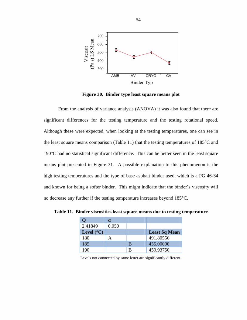
54

Figure 30. Binder type least square means plot

From the analysis of variance analysis (ANOVA) it was also found that there are

significant differences for the testing temperature and the testing rotational speed.

Although these were expected, when looking at the testing temperatures, one can see in

the least square means comparison (Table 11) that the testing temperatures of 185°C and

190°C had no statistical significant difference. This can be better seen in the least square

means plot presented in Figure 31. A possible explanation to this phenomenon is the

high testing temperatures and the type of base asphalt binder used, which is a PG 46-34

and known for being a softer binder. This might indicate that the binder’s viscosity will

no decrease any further if the testing temperature increases beyond 185°C.

Table 11. Binder viscosities least square means due to testing temperature

Q α

2.41849 0.050

Level (°C) Least Sq Mean

180 A 491.80556

185 B 455.00000

190 B 450.93750


55

Figure 31. Testing temperature least square means plot

Table 12 and Figure 32 present the least square means comparisons of the binder

viscosities due to testing rotational speed factor. It is observed that the viscosities for

each level of this factor are statistically different between them as expected. The higher

the testing rotational speed the lower the viscosity of the binder, due to the high shear

stresses at which the binder is being subjected.

Table 12. Binder viscosities least square means due to testing rotational speed

Q α

2.41849 0.050

Level (rpm) Least Sq Mean

10 A 549.65278

20 B 465.45139

50 C 382.63889


Figure 32. Testing speed least square means plot

56

The analysis of variance (ANOVA) table also shows that the interaction between

the binder type and the testing rotational speed is statistically significant. Figure 33

presents the least square means plot for this interaction. The slopes of the viscosities for

each type of binder at the testing rotational viscosities confirm that there is interaction

between these two factors, because none of the slopes are parallel.

Figure 33. Binder type * speed least square means plot

Dynamic Shear Rheometer (DSR)

Each of the four binders was tested at high and low temperatures in the Dynamic

Shear Rheometer. The rheological properties of unaged and RTFO aged samples of the

four binders were evaluated for high temperatures. Meanwhile, the rheological properties

of PAV aged samples were evaluated at low temperatures. From the results of the

rheological properties, continuous grading of the four binders can be performed.

High Temperatures

The results obtained from the DSR testing at high temperatures are presented in

Table 13. Results on the continuous grading for the base asphalt PG46-34 (presented

57

elsewhere) are also shown in aforementioned table as comparison on how ground tire

rubber (GTR) can increase the binder’s rheological properties at high temperatures.

From Table 13 it can be seen that unaged ambient GTR binder high continuous

grading is 0.6 degrees higher compared to the unaged cryogenic GTR binder. When

comparing the effect of PO on the unaged asphalt rubber blends, it can be seen that PO

will increase the continuous grading for both ambient and cryogenic GTR blends.

Table 13. High temperature continuous grading of binders

High Temperature

Continuous Grading, °C

Blend Type Unaged RTFO Aged

PG 46-34 50.9 53.0

Amb 66.7 67.0

AV 67.2 68.3

Cryo 66.1 66.7

CV 66.5 67.9

As for the RTFO aged material, it is expected that the resulting grading would be

higher than for the unaged material, this trend is observed for all the binders. However,

even though the binders with PO became stiffer after being RTFO aged, with respect to

their respective unaged binder, the magnitude of how much stiffer they got is higher than

the binders that did not have PO. These differences can be easily observed in Figure 34.

58

Figure 34. High temperature continuous grading

From Figure 34, it can also be observed how the two types of ground tire rubber

increased the performance grading on the high temperature of the base asphalt, an

increase in three grades, from being a PG46 to a PG64.

Intermediate Temperatures

The binders were tested in the dynamic shear rheometer (DSR) after being PAV

aged at 100°C, at intermediate temperatures as required by the AASHTO M320 standard

specification (2010) to be able to grade the binders. The results from the DSR are

tabulated in Table 14. Due to equipment constraints all the binders were tested just from

16°C until 7°C, most of the samples did not fail at 7°C, except for two samples. Thus,

the results were averaged and the failure temperatures for those samples that did not fail

at 7°C were estimated. Likewise for high temperatures, Table 14 also presents the

intermediate temperature grading for the PAV aged material of the base binder PG46-34

46 52 58 64 70

PG 46-34

Amb

AV

Cryo

CV

High Temperature, °C

Bin

der

Ty

pe

Unaged

RTFO Aged

59

reported elsewhere, so it can be observed how GTR affects the intermediate temperature

grading on the binders.

Table 14. Intermediate temperature continuous grading of PAV aged binders

Intermediate

Temperature


Blend Type PAV Aged

PG 46-34 9.0

Amb 5.7

AV 6.8

Cryo 6.4

CV 6.8

From Table 14, it can be seen how both GTRs improve the intermediate

temperature grading of the binders by lowering the continuous performance grade.

However, it seems that ambient GTR lowers the continuous grading a bit more than

cryogenic GTR does. When looking at the effects of PO on the asphalt rubber blends, it

is noticeable that it causes an increase on the intermediate continuous grading of the

binders, however it does not affect the final performance grading because all the binders

will have to be reported as being a 7°C PAV intermediate temperature grade. Figure 35

illustrates graphically the trends mentioned, it can also be observed how the GTR

increases by one grade the intermediate temperature performance of the base binder

PG46-34, that had an original PAV intermediate temperature grade of 10°C.

60

Figure 35. Intermediate temperature continuous grading for PAV Aged binders

Mass Loss

After performing the RTFO aging procedure, the mass loss of the four types of

binder was computed, and these are tabulated in Table 15. The percentage mass losses

obtained for the asphalt rubber binders with PO did not meet the specified mass loss

criteria of no more than one percent of mass loss in AASHTO M320 standard

specification for binder grading. The percentage mass loss of the base asphalt PG 46-34

reported elsewhere is presented as general reference.

Table 15. Summary of average percentage mass loss

Binder Type Average % Mass Loss

PG 46-34 0.43%

AMB 0.86%

AV 1.24%

CRYO 0.81%

CV 1.28%

1 4 7 10 13 16

PG 46-34

Amb

AV

Cryo

CV

Intermediate Temperature, °C

Bin

der

Ty

pe

PAV aged

61

From the results presented in Table 15, it can be thought that PO increases the

mass loss in the binders, this trend is observed in both types of GTR binders. Figure 36

illustrates graphically the mass loss percentage of the four types of RTFO aged asphalt

rubber binders. However, it is believe that the high percentage of mass loss for the four

types of binders is not completely due to the evaporation of the volatiles in the asphalt

rubber, but due to swelling of the rubber while in the RTFO oven. This swelling can

make the asphalt rubber film that coats the bottles during the test to be thicker and

somehow making the binder to overflow the bottles, and thus binder is spilled inside the

oven during the test. One can hypothesize that this swelling is increased when PO is

added, promoting more spillage of the binder during the testing.

Bending Beam Rheometer (BBR)

The results obtained from the Bending Beam Rheometer (BBR) testing are

summarized in Table 16. The continuous grading for low temperature of the base asphalt

PG 46-34 was reported elsewhere, and it is just presented as a general reference.

Figure 36. Average percentage mass loss

0.86%

1.24%

0.81%

1.28%

0.43%

0.00%

0.20%

0.40%

0.60%

0.80%

1.00%

1.20%

1.40%

1.60%

1.80%

Average % Mass Loss

% M

ass

Lo

ss

Mix Type

AMB

AV

CRYO

CV

PG 46-34

62

Table 16. Low Temperature continuous grading of binders

Low Temperature


Blend Type BBR results

PG 46-34 -36.2

Amb -38.9

AV -37.8

Cryo -37.3

CV -35.8

The two binders that contained PO graded lower when compared with their

respective type of binder but without PO. The resistance to thermal cracking is somehow

affected with the addition of PO to the asphalt rubber. However, the performance grade

for the four types of asphalt rubber binders was not affected, remaining a -34

performance grade for creep stiffness. It is known that when binders are polymer

modified the performance of the binder can improve on one side of the temperature (high

or low), but for the other temperature (low or high) the performance typically diminishes.

This situation was not observed for the binders in this study.

Figure 37 shows that the binder with ambient GTR had the better thermal

cracking temperature performance of the four binders, and the binder with cryogenic

GTR and PO had reduced thermal cracking temperature performance of the these binders.

63

Figure 37. BBR low temperature continuous grading

Asphalt Binders Master Curves

Frequency sweeps were performed for each type of asphalt rubber binder through

a DSR, the results obtained were used to construct the master curves of the unaged,

RTFO aged and PAV aged binders for the rheological property of the complex modulus

G*. These master curves were all developed using a reference temperature of 20°C and

are presented in Figures 36 through 38.

The four unaged asphalt rubber binders presented similar rheological performance

for their complex modulus (G*) at low, intermediate and high temperatures. However, it

is noticeable that the cryogenic GTR binder presents somewhat lower complex modulus

values compared to the other three asphalt rubber binders, this difference in stiffness is

more noticeable at high temperatures. In contrast, the cryogenic GTR and PO binder

behaves stiffer than its version without PO, the increase in stiffness can be due to the

addition of PO. However, this trend was not observed for the asphalt rubber with

-40 -34 -28

PG 46-34

Amb

AV

Cryo

CV

Low Temperature, °C

Bin

der

Ty

pe

BBR

64

ambient GTR, since the master curves of both binders, with and without PO are one over

the other. For RTFO aged materials, as expected the complex modulus for the four

asphalt rubber binders increased, meaning that the binders got stiffer due to aging. The

same trend observed for the unaged materials was observed for the RTFO aged materials,

being cryogenic GTR softer than the rest of the asphalt rubber binders, which will impact

negatively the performance of the binder for rutting resistance.

The trend observed in the unaged and RTFO aged materials, of the cryogenic

GTR binder, being softer than the rest of the asphalt rubber binder is observed as well for

the PAV aged materials. The complex modulus for the four asphalt rubber binders

increased as expected due to the PAV aging.

One possible explanation on why PO seems to affect only the stiffness of the

cryogenic asphalt rubber rather than both types of GTRs can be due to the difference in

size distributions of the rubbers; cryogenic GTR is a finer material than ambient GTR

which makes it easier for the PO to interact with it than with ambient GTR.

65

Figure 38. Master curves of Unaged asphalt rubber binders

1.E+0

1.E+1

1.E+2

1.E+3

1.E+4

1.E+5

1.E+6

1.E+7

1.E+8

1.E

-6

1.E

-5

1.E

-4

1.E

-3

1.E

-2

1.E

-1

1.E

+0

1.E

+1

1.E

+2

1.E

+3

Co

mp

lex M

od

ulu

s, G

* (

Pa

)

Frequency, Hz

AMB

AV

CRYO

CV

65

66

Figure 39. Master curves of RTFO asphalt rubber binders

1.E+0

1.E+1

1.E+2

1.E+3

1.E+4

1.E+5

1.E+6

1.E+7

1.E+8

1.E

-6

1.E

-5

1.E

-4

1.E

-3

1.E

-2

1.E

-1

1.E

+0

1.E

+1

1.E

+2

1.E

+3

Co

mp

lex M

od

ulu

s, G

* (

Pa

)

Frequency, Hz

AMB

AV

CRYO

CV

66

67

Figure 40. Master curves of PAV Aged asphalt rubber binders

1.E+0

1.E+1

1.E+2

1.E+3

1.E+4

1.E+5

1.E+6

1.E+7

1.E+8

1.E

-6

1.E

-5

1.E

-4

1.E

-3

1.E

-2

1.E

-1

1.E

+0

1.E

+1

1.E

+2

1.E

+3

Co

mp

lex M

od

ulu

s, G

* (

Pa

)

Frequency, Hz

AMB

AV

CRYO

CV

67

68

Mixes Performance Testing Results

Dynamic Modulus (E*)

The results of the dynamic modulus (E*) for the four asphalt rubber mixtures are

tabulated in Table A. 1 to Table A. 4 in Appendix A. From these results the master

curves for the four types of asphalt rubber mixtures were constructed and are presented

and discussed in the next section of this chapter.

The greyed values in the appendix tables were considered outliers and were not

taken into consideration to build the master curves of the four asphalt rubber mixtures.

The criteria used to determine if a value was considered to be an outlier, was to look up at

the coefficient of variation, if it was higher than twelve percent, then the smaller value

was not taken into consideration for the average used in the master curves construction.

This procedure was performed for the ambient GTR and PO mixture and the

cryogenic GTR mixture. Thereby coefficients of variations lower than twelve percent

were obtained by applying this method to the ambient GTR and PO mixture. However,

for the cryogenic GTR mixtures the two smaller values were ignored for the average used

to build its master curve, due to the high variability that these two values were

introducing to the average. It should be noted that the averages and coefficient of

variation reported in the appendix tables do take into consideration these values.

Asphalt Rubber Mixtures Master Curves

After taking care of the possible outliers in the data, the procedure described in

the standard practice AASTHO PP62 (2010) was followed to construct the master curves

of the asphalt rubber mixtures. The second-order polynomial equation described in

69

aforementioned standard practice was used to find the shifting factors to reduce the nine

frequencies of the test. A reference temperature of 21°C was used to build the master

curves, therefore the related frequencies of the temperatures 4°C and 37°C were shifted,

to the right and to the left, respectively, to obtain the master curves.

Figures 33 to 36 illustrate the data before and after being shifted for the four types

of asphalt rubber mixtures. For a better comparison Figure 45 presents the four master

curves together, from this figure it can be seen that the behavior of the four asphalt rubber

mixtures are very similar at low and intermediate temperatures, however it seems that for

high temperatures the ambient GTR mixtures performs a little bit better than the other

three asphalt rubber mixtures. To see if there is any statistically significant diference a

statistical analysis was performed for each testing temperature at a certain frequency.

This is, for the data at a testing temperature of 4°C which is located at the farther right

side of the master curves and that is related to high frequencies and low temperatures, the

analysis was performed at the 25 Hz frequency. As for the testing temperature of 21°C,

which is the reference temperature and which values are located in the middle of the

master curve, is related to the intermediate frequencies and temperatures, thus the data at

the frequency of 10 Hz was chosen. For the data at a testing temperature of 37°C, that is

located at the farther left side of the master curves belongs to the lower frequencies and

high temperatures, thus the lower testing frequency of 0.1 Hz was pick to be analyzed.

Table 17 presents the results obtained from the ANOVA analysis, which showed

that no significant difference was observed between the mix types at the determined

frequency and at that specific testing temperature. Thus, it can be inferred that the four

70

asphalt rubber mixtures will have a similar performance at low, intermediate and high

frequencies.

Figure 41. Master curve of AMB Mix

1.E+2

1.E+3

1.E+4

1.E+5

1.E

-3

1.E

-2

1.E

-1

1.E

+0

1.E

+1

1.E

+2

1.E

+3

1.E

+4

|E*

|, M

Pa

Frequency, Hz

4°C

4°C shifted

21°C

37°C

37°C shifted

Fit

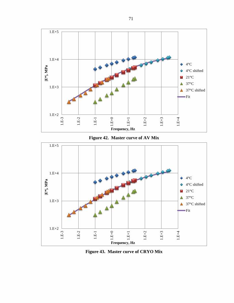
71

Figure 42. Master curve of AV Mix

Figure 43. Master curve of CRYO Mix

1.E+2

1.E+3

1.E+4

1.E+5

1.E

-3

1.E

-2

1.E

-1

1.E

+0

1.E

+1

1.E

+2

1.E

+3

1.E

+4

|E*

|, M

Pa

Frequency, Hz

4°C

4°C shifted

21°C

37°C

37°C shifted

Fit

1.E+2

1.E+3

1.E+4

1.E+5

1.E

-3

1.E

-2

1.E

-1

1.E

+0

1.E

+1

1.E

+2

1.E

+3

1.E

+4

|E*

|, M

Pa

Frequency, Hz

4°C

4°C shifted

21°C

37°C

37°C shifted

Fit

72

Figure 44. Master curve of CV Mix

Figure 45. Comparison between master curves mixtures

1.E+2

1.E+3

1.E+4

1.E+5

1.E

-3

1.E

-2

1.E

-1

1.E

+0

1.E

+1

1.E

+2

1.E

+3

1.E

+4

|E*

|, M

Pa

Frequency, Hz

4°C

4°C shifted

21°C

37°C

37°C shifted

Fit

1.E+2

1.E+3

1.E+4

1.E+5

1.E

-3

1.E

-2

1.E

-1

1.E

+0

1.E

+1

1.E

+2

1.E

+3

1.E

+4

|E*

|, M

Pa

Frequency, Hz

AMB

AVR

CRYO

CV

73

Table 17. Dynamic modulus ANOVA table

Dynamic modulus at 4°C for high frequency

Source DF Sum of Squares Mean Square F Ratio Prob > F

Mix Type 3 3167544 1055848 0.5074 0.6827

Error 16 33295947 2080997

C. Total 19 36463491

Dynamic modulus at 21°C for intermediate frequency


Mix Type 3 505744.4 168581 0.5969 0.6261

Error 16 4518515.6 282407

C. Total 19 5024260.0

Dynamic modulus at 37°C for low frequency


Mix Type 3 10397.106 3465.70 1.4216 0.2732

Error 16 39006.016 2437.88

C. Total 19 49403.122

Flow Number (FN)

After performing the dynamic modulus test, the same specimens were then tested

for flow number at a testing temperature of 37°C. The flow number test is an indicative

of the rutting performance of the asphalt mixes. The higher the flow number, the better

rutting performance the mix is supposed to have. The results obtained from the test are

presented in Appendix B. It should be noted that one outlier for each mix type was not

taken into consideration to obtain the average flow number of each mix; these values are

shown in gray in Table B. 1, and were not included in the statistical analysis performed.

Figure 46 shows the results obtained from the testing of the four asphalt rubber mixtures.

Cryogenic GTR mixture had the lowest flow number from all the asphalt rubber

mixtures, this result goes along with the results obtained from the DSR testing for at high

temperatures and from the binder master curve. Likewise the high flow number obtained

74

for the ambient GTR mixtures relates with the results from the binder testing, having

these higher stiffness when compared to cryogenic GTR mixtures.

Figure 46. Average Flow Number

A statistical analysis was performed in order to see if these differences between

flow numbers are statistically significant. Tables 17 and 18 summarize the statistics

performed for the flow number results and show that there is a significant difference

between the mix types due to the p-value of 0.0001, and that the mix types that are

different amongst them are the mixes containing ambient GTR and cryogenic GTR,

although no difference was found between the mixes with or without PO.

Table 18. Flow number ANOVA table


Mix Type 3 9133005 3044335 16.6908 0.0001*

Error 12 2188757 182396

C. Total 15 11321762


3607 3321

1805 2174

0

500

1000

1500

2000

2500

3000

3500

4000

4500

Average FN

Flo

w N

um

ber

Mix Type

Amb

AV

Cryo

CV

75

Table 19. Flow number least square means differences

q* Alpha

2.96880 0.05

Level Mean

AMB A 3607.25

AV A 3320.50

CV B 2173.75

CRYO B 1805.00


Tensile Strength Ratio (TSR)

The tensile strength ratio (TSR) of two sets of three samples each, one

conditioned and the other non-conditioned, for each asphalt rubber mixture were obtained

by means of the indirect tensile test. Figure 47 illustrates the results from the tensile

strength ratio. It should be noted that the four ratios were higher than 1.0, in normal

circumstances it is expected that the ratio of the conditioned versus non-conditioned

samples would give a ratio lower than 1.0, being 0.80 the lower accepted boundary for

reasonable performance, however this was not observed. Cryogenic GTR mixture

presented the highest ratio from the set of asphalt rubber mixtures to be tested. In

contrast with ambient GTR that had the lowest ratio from the mixtures tested, very much

similar to the cryogenic GTR and PO mixture.

76

Figure 47. Average Tensile Strength Ratios

A statistical analysis was performed to determine if the differences in tensile

strength ratio between mix types were significant, the ANOVA table is shown in Table

20, where it can be seen that the differences in tensile strength ratio are not statistically

significant since the p-value obtained from the statistical analysis of 0.5197 is very high

compared to the alpha value of 0.05 used in the statistical analysis.

Table 20. Tensile strength ratio ANOVA table


Mix Type 3 0.02608656 0.008696 0.8173 0.5197

Error 8 0.08511266 0.010639

C. Total 11 0.11119923

The peak loads of the specimens were also analyzed statistically to see if the was

a statistical significant difference between mixes and to see the effects of the treatment

(conditioned versus dry specimens) had any influence in the peak loads. Table 21

presents the results of the ANOVA analysis, from where it can be inferred that there is no

1.19 1.26

1.31

1.20

0.80

0.90

1.00

1.10

1.20

1.30

1.40

1.50

1.60

TSR Average

Ten

sile

Str

eng

th R

ati

o

Mix Type

Amb

AV

Cryo

CV

77

statistical difference amongst the mix types due to the high p-value of 0.3175; however,

the treatments (conditioned versus dry) presented a statistical significant difference, as

shown by the p-value obtained of less than 0.0001. The least square means plot in Figure

48 shows that the conditioned specimens presented higher mean average on the peak

load, than the dry (non-conditioned) specimens.

Table 21. Peak load ANOVA table

Source DF Sum of

Squares Mean Square F Ratio Prob > F

Mix Type 3 0.9537108 0.317904 1.2721 0.3175

Treatment 1 9.8880844 9.888084 39.5664 <.0001*

Mix Type*Treatment 3 0.3396968 0.113232 0.4531 0.7187

Error 16 3.998581 0.24991 6.3917

C. Total 23 15.180073


It is hypothesized that there is an interaction between the rubber and the base

asphalt when subjected to moisture conditioning; this can be due to the elastic properties

of the rubber that can make the mixes in general to withstand more strains without failing

and somehow when the rubber mixtures were subjected to moisture conditioning a

rejuvenator reaction occurred to the mixes. However, it seems that the addition of PO

does not influence this behavior, since no statistical differences were found between the

mixes.

78

Figure 48. Treatment least square means plot for peak load

It should be mentioned that none to almost no stripping was observed during the

inspection of the broken samples after the indirect tensile strength test, as it can be seen

from Figure 49. The light spots in the figure are broken aggregates, most of the samples

failed through the interface of the binder and the aggregates, but as said before no

stripping was observed.

Figure 49. Indirect tensile strength specimens tested

79

CHAPTER 5. CONCLUSIONS AND RECOMMENDATIONS

This research has determined how the addition of 4.5 percentage of

polyoctenamer (PO) by weight of ground tire rubber (GTR) influences the rheological

properties and performance of asphalt rubber binders laboratory-produced with a base

asphalt PG46-34 and two different ground tire rubbers at 12 percent by weight of asphalt,

ambient GTR and cryogenic GTR. Likewise, the performance of their respective asphalt

rubber mixtures, mixed and compacted in laboratory, was also evaluated. The aggregate

gradation and binder content of the laboratory-produced asphalt rubber mixtures were

kept the same throughout the course of this research.

Binders

The validation of the research hypothesis about the influence of the addition of

PO to asphalt rubber binders over their viscosity was corroborated. The viscosities of the

asphalt rubber binders containing PO were found statistically different from the asphalt

rubber binders without PO for alpha equals to 0.05. It was also found that the viscosities

of the two asphalt rubber binders with PO where statistically different between them,

whereas the viscosities of the two asphalt rubber binders without PO were not statistically

different between them.

Although the statistical analysis showed that the addition of PO will indeed

decrease the viscosity of the asphalt rubber binders, the amount of reduction in viscosity

was not enough to meet the criteria for the mixing and compaction viscosities ranges

established in the performance-graded asphalt binder specification (SuperPave).

However, it is believe that the high viscosity readings were due to the particle effect of

the rubbers during the viscosity testing, leading to higher viscosity values than those that

80

would be obtained if only the liquid part was tested. Thus, it is recommended to

reevaluate the viscosities of just the liquid part of the asphalt rubber binder to avoid

having the particle effects of the rubber influencing the viscosity readings, and to see if

the new viscosities meet the SuperPave binder specification criteria, and new mixing and

compaction temperatures can be determine.

The final performance grading for high temperature performance of the four types

of asphalt rubber binders were found to be the same for the high temperature, PG64, thus

it is concluded that the addition of PO will not affect the final grading for high

temperature of asphalt rubber binders. However, the predicted continuous grading of the

asphalt rubber binders without PO showed lower performance grading than the predicted

continuous grading of the asphalt rubber binders with PO, this difference being about half

degree for the unaged materials and one degree for the RTFO aged materials.

The low temperatures for the final performance grading for the PAV aged of the

four asphalt rubber binders in the DSR was determined to be 7°C. However, the

predicted continuous grading revealed that the low temperature for the PAV aged

materials of the asphalt rubber binder containing ambient GTR where around one degree

different, having the binder with PO the higher temperature. This means that the addition

of PO reduced the low temperature performance of the PAV aged materials by one

degree. While the difference between the asphalt rubber binders containing cryogenic

GTR was less than half degree, the same trend of the binder with PO diminishing the low

temperature performance was found.

The mass loss results for the asphalt rubber binders with PO were higher than the

criteria established in the performance-graded asphalt binder specification (more than 1.0

81

percent). This can be explained due to more swelling of the rubber particles during the

aging process. It is suspected that PO interacts in some way with the rubber promoting

more the swelling of the rubber particles, causing spillage of binder out of the RTFO

bottles during the aging process. It is recommended to try with less amount of binder per

bottle, instead of 35 grams, to confirm this hypothesis.

The final low temperature performance grading for the PAV aged materials in the

BBR was found to be a PG -34 for the four types of asphalt rubber binders. However, for

the continuous grading, the asphalt rubber binders without PO had better performance at

low temperatures than the binders with PO; the differences were about one degree of

temperature. Also, the asphalt rubber binders containing cryogenic GTR had lower

performance compared with the asphalt rubber binders having ambient GTR.

The master curves obtained from the results of the testing for the four asphalt

rubber binders showed that the behavior of the asphalt rubber binders is very similar

between them. Being the binders containing ambient GTR somewhat stiffer that the

binders with cryogenic GTR.

The binders study performed in this research did not include separation tests on

the laboratory-produced binders, it is recommended to evaluate in future research how

the addition of PO can influence over the stability of asphalt rubber binders.

Mixes

The results from the dynamic modulus testing were used to construct the mixtures

master curves. The statistical analysis performed to test the research hypothesis revealed

82

that the addition of the PO did not influence the low, intermediate and high temperatures

performance of the mixtures prepared with the four types of asphalt rubber binders.

The flow number test revealed that the rutting performances of the asphalt rubber

mixes were not different between the mixes with the same type of ground tire rubber.

Thus, statistically the performance of the asphalt rubber mixes containing PO is no

different from the mixes without it. However, the statistical analysis showed that the type

of ground tire rubber will influence the rutting performance; having the ambient GTR

mixes better rutting performance than the cryogenic GTR mixes.

The tensile strength ratio was found not to be different for the four types of

asphalt rubber mixes. Thus the addition of PO does not affect the moisture susceptibility

of asphalt rubber mixes.

This study did not include fatigue cracking performance testing of the asphalt

rubber mixes by means of the beam fatigue test; it is recommended that testing for fatigue

performance should be done in the future to evaluate the influence of PO over the

performance of the asphalt rubber mixtures.

It is also recommended to evaluate the fracture resistance of the asphalt rubber

mixes by means of the semi-circular bend geometry (SCB) test and study the influence of

PO over the asphalt rubber mixes at low temperatures.

83

REFERENCES

AASHTO. (2010). Designation M 320-10 Performance-Graded Asphalt Binder Standard

Specifications for Transportation Materials and Methods of Sampling and

Testing, 27th Ed. Washington, D.C.: American Association of State Highway and

Transportation Officials

AASHTO. (2010). Designation M 323-07 Superpave Volumetric Mix Design Standard




AASHTO. (2010). Designation PP 60-09 Preparation of Cylindrical Performance Test

specimens Using the Superpave Gyratory Compactor (SGC) Standard




AASHTO. (2010). Designation PP 62-10 Developing Dynamic Modulus Master Curves

for Hot Mix Asphalt (HMA) Standard Specifications for Transportation Materials

and Methods of Sampling and Testing, 27th Ed. Washington, D.C.: American

Association of State Highway and Transportation Officials

AASHTO. (2010). Designation R 28 Accelerated Aging of Asphalt Binder Using a

Pressurized Aging Vessel (PAV). Standard Specifications for Transportation

Materials and Methods of Sampling and Testing, 27th Ed. Washington, D.C.:

American Association of State Highway and Transportation Officials.

AASHTO. (2010). Designation R 30-02 (2006) Mixture Conditioning of Hot Mix Asphalt

(HMA) Standard Specifications for Transportation Materials and Methods of

Sampling and Testing, 27th Ed. Washington, D.C.: American Association of State

Highway and Transportation Officials

AASHTO. (2010). Designation R 35-09 Superpave Volumetric Design for Hot Mix

Asphalt Standard Specifications for Transportation Materials and Methods of

Sampling and Testing, 27th Ed. Washington, D.C.: American Association of State

Highway and Transportation Officials

AASHTO. (2010). Designation T 240 Standard Method of Test for Effect of Heat and Air

on a Moving Film of Asphalt Binder (Rolling Thin-Film Oven Test). Standard


Testing, 27th

Ed. Washington, D.C.: American Association of State Highway and

Transportation Officials.

AASHTO. (2010). Designation T 283-07 Resistance of Compacted Hot Mix Asphalt

(HMA) to Moisture Induced Damage. Standard Specifications for Transportation

84

Materials and Methods of Sampling and Testing, 27th Ed. Washington, D.C.:

American Association of State Highway and Transportation Officials

AASHTO. (2010). Designation T 313 Determining the Flexural Creep Stiffness of

Asphalt Binder Using the Bending Beam Rheometer (BBR). Standard


Testing, 27th

Ed. Washington, D.C.: American Association of State Highway and


AASHTO. (2010). Designation T 315 Standard Method of Test for Determining the

Rheological Properties of Asphalt Binder Using a Dynamic Shear Rheometer

(DSR). Standard Specifications for Transportation Materials and Methods for

Sampling and Testing, 27th

Ed. Washington D.C.: American Association of State

Highway and Transportation Officials.

AASHTO. (2010). Designation T 316 Standard Method of Test for Viscosity

Determination of Asphalt Binder Using Rotational Viscometer. Standard




AASHTO. (2010). Designation TP 62-07 Determining Dynamic Modulus of Hot Mix

Asphalt (HMA) Standard Specifications for Transportation Materials and Methods

of Sampling and Testing, 27th Ed. Washington, D.C.: American Association of

State Highway and Transportation Officials

Anderson, C. (1991). Evaluation of recycled rubber in asphalt concrete / by Chris

Anderson. Ames, Iowa: Ames, Iowa : Iowa Dept. of Transportation, Highway

Division, Office of Materials.

Anderson, C. (1992a). Evaluation of recycled rubber in asphalt concrete, Black Hawk

County / by Chris Anderson. Ames, Iowa: Ames, Iowa : Office of Materials,

Highway Division, Iowa Dept. of Transportation.

Anderson, C. (1992b). Evaluation of recycled rubber in asphalt concrete, Black Hawk

County construction report for Iowa Highway Research Board project HR-330B /

by Chris Anderson. Ames, Iowa: Ames, Iowa : Iowa Dept. of Transportation,

Highway Division.

Anderson, C. (1992c). Evaluation of recycled rubber in asphalt concrete, Dubuque

County construction report for Iowa Highway Research Board project HR-330C /

Chris Anderson. Ames, Iowa: Ames, Iowa : Iowa Dept. of Transportation,

Highway Division.

Anderson, C. (1992d). Evaluation of recycled rubber in asphalt concrete, Plymouth

County construction report for Iowa Highway Research Board project HR-330A /

85

Chris Anderson. Ames, Iowa: Ames, Iowa : Iowa Dept. of Transportation,

Highway Division.

Anderson, C. (1993). Asphalt rubber cement concrete, Webster County construction

report for Iowa Department of Transportation project HR-555 / by Chris

Anderson. Ames, Iowa: Ames, Iowa : Iowa Dept. of Transportation, Highway

Division.

Anderson, C. (1994). Production of asphalt rubber concrete by the dry process / by Chris

Anderson. Ames, Iowa: Ames, Iowa : Iowa Dept. of Transportation.

Asphalt Institute (2001). Performance graded asphalt binder specification and testing

Superpave Series No.1 (SP-1) Asphalt Institute. Third Edition. Lexington, KY

Asphalt Institute (2001). Superpave Mix Design. Superpave Series No.2 (SP-2) Third

Edition. Asphalt Institute. Lexington, KY

ASTM Standard D70 (1997). Standard Test Method For Specific Gravity And Density Of

Semi Solid Bituminous Materials (Pycnometer Method). ASTM International,

West Conshohocken, PA, 1997

ASTM Standard D4402 (2002). Standard Test Method for Viscosity Determination of

Asphalt at Elevated Temperatures Using a Rotational Viscometer. ASTM

International, West Conshohocken, PA, 2002

ASTM Standard D6814 (2002). Standard Test Method for Determination of Percent

Devulcanization of Crumb Rubber Based on Crosslink Density. ASTM

International, West Conshohocken, PA, 2002

Bahia, H.U., and R. Davies (1994). Effect of Crumb Rubber Modifiers (CRM) on

Performance-Related Properties of Asphalt Binders. Journal of the Association

of Asphalt Paving Technologies, Vol. 64, 1994

Bausano, J. and Williams R.C. (2010). Energy-based Approach for Determining Flow

Number. Journal of Testing and Evaluation, 2010, Vol.38(1), pp. 111-118

Bennert, T. (2001). Performance evaluation of TOR (TOR) using dry and wet mixing

processes in hot mix asphalt. Asphalt/Pavement Laboratory (RAPL). Rutgers

University. Piscataway, NJ.

Burns, B. (2000). Rubber-modified asphalt paving binder. EP 0994161 A2, filed Oct 13

1999, and issued Apr 19, 2000.

Burns, B. (2004). Modification of rubberized asphalt with polyoctenamer. Symposium,

Cheyenne, June 23-25 Wyoming, 2004.

86

Corbett, L. W. (1970). Relationship between composition and physical properties of

asphalt. Proceedings of American Association of Asphalt Paving Technologits,

Vol.39, pp. 481-491.

Epps, J.A. (1994). Uses of Recycled Rubber Tires in Highways. NCHRP Synthesis of

Highway.

Practice nº 198, Transportation Research Board, Washington, D.C., USA.

Estakhri, C. K. et al (1992). Use, Availability, and Cost-Effectiveness of Asphalt Rubber

in Texas. Transportation Research Record No. 1339, Transportation Research

Board, Washington, DC, 1992.

FHWA (1995). Crumb rubber modifier (CRM) in asphalt pavement summary of

practices in Arizona, California and Florida. Washington, D.C. Federal Highway

Administration.

FHWA (2008). User Guidelines for Byproduct and Secondary Use Materials in

Pavement Construction. FHWA-RD-97-148. Washington, D.C. Federal Highway

Administration.

Fontes, L. (2009). Optimização do desempenho de misturas betuminosas com betume

modificado com borracha para reabilitação de pavimentos. Escola de

Engenharia. Universidade do Minho.

Hamed, G.R. (1992). “Materials and Compounds” Engineering with Rubber - How to

Design Rubber Components (2nd edition), from Alan N. Gent, Hanser Publishers.

Heitzman, M. (1992). State of the practice: design and construction of asphalt paving

materials with crumb rubber modifier. Publication No. FHWA-SA-92-022, US

Dept. of Transportation, Federal Highway Administration

Heitzman, M. A. (1992). State of the practice : design and construction of asphalt

paving materials with crumb rubber modifier. Washington, D.C. U.S. Dept. of

Transportation, Federal Highway Administration, Office of Engineering, Office

of Technology Applications.

Hicks, R.G. (2002). Asphalt Rubber Design and Construction Guidelines. Volume I –

Design Guidelines. Northern California Asphalt Concrete Technology Center.

California Integrated Waste Management Board. January 2002

Hicks, R.G. and Epps, J.A. (2000). Quality control for asphalt rubber binders and mixes.

Rubber Pavement Association. Tempe, Arizona, USA

Ichniowski, T. (1993). Noises in the House over rubber in the road. Engineering News

Record. May 24, 1993. pp. 24,25.

87

Iowadnr.gov (2013). Tires. [online] Available at: http://www.iowadnr.gov/Environment/

LandStewardship/WasteManagement/Tires.aspx [Accessed: 24 Apr 2013].

Isayev, A.I. (2005). “Recycling of Rubbers” Science and Technology of Rubber (3rd

Edition). Elsevier.

Kandhal, P.S. (1993). Waste materials in hot-mix asphalt – An overview. Use of waste

materials in hot-mix asphalt. ASTM STP1193, H. Fred Waller, American Society

for Testing and Materials. Philadelphia, 1993.

Lesueur, D. (2009). The colloidal structure of bitumen: consequences on the rheology

and on the mechanisms of bitumen modification. Advances in Colloid and

Interface Science, 2009, vol.145(1), pp 42-82.

Li, Xinjun and Williams, R.C. (2012). A practical Dynamic Modulus Testing Protocol.

Journal of Testing and Evaluation, 2012, Vol.40(1), pp. 103002

Liu, S. (2013). Influence of Different Factors of Crumb Rubber on the Properties of

Crumb Rubber Modified Asphalt. Asian Journal of Chemistry, 25(3), 1583-1586.

Mark, James E.; Erman, Burak; Eirich, Frederick R. (2005). Science and Technology of

Rubber (3rd Edition). Elsevier.

McGennis, R. B. (1995). Evaluation of Physical Properties of Fine Crumb Rubber-

Modified Asphalt Binders. Transportation Research Board, 1995

NCHRP (2002). Report 465. Simple Performance Test for Superpave Mix Design.

Washington 2002

NCHRP (2003). Report 513. Simple Performance Tester for Superpave Mix Design:

First-Article Development and Evaluation. Washington 2003

NCHRP (2005). Report 547. Simple Performance Tests: Summary of Recommended

Methods and Database. Washington 2005

NICNAS (1999). Cyclooctene homopolymer. Full Public Report. National Industrial

Chemicals Notification and Assessment Scheme. October, 1999

Oyenkule, L.O. (2007). Influence of Chemical Composition on the Physical

Characteristics of Paving Asphalts. Petroleum Science and Technology,

Vol.25(11), pp. 1401-1414.

Peralta, E.J.F. (2009). Study of the interaction between Bitumen and Rubber. Escola de

Engenharia. Universidade do Minho

Rahman, M.M. (2004). Characterization of Dry Process Crumb Rubber Modified

Asphalt Mixtures. School of Civil Engineering, University of Nottingham

88

Recycling Research Institute (2006). Rubber Recycling. Scrap Tire News. Recycling

Research Institute. Leesburg, Virginia, USA

Reschner, K. (2006). Scrap Tire Recycling – A summary of Prevalent Disposal and

Recycling Methods. Berlin, Germany. 2006

Roberts, F. et al (2009). Hot mix asphalt materials, mixture design and construction.

Lanham, Md. Napa Educational Foundation

Robinette, C. and Williams, R.C. (2006). The effects of the testing history and

preparation method on the superpave simple performance test, Journal of the

Association of Asphalt Paving Technologist, Vol. 75, 297-317, 2006

Rubber Manufacturers Association (2009). Scrap tire markets in the United States. 9th

Biennial Report. May 2009

Rubberasphaltsolutions.com (2010) Rubber Asphalt Solutions LLC. [online] Available

at: http://rubberasphaltsolutions.com/reference.htm [Accessed: 15 Feb 2013].

Shuler, T. S. et al (1986). Investigation of materials and structural properties of

asphalt-rubber paving mixtures. Federal Highway Administration, Research,

Development, and Technology ; Springfield, Va.

Solaimanian, M. et al (2003). Evaluation of TOR Reactive Modified in Crumb Rubber

Asphalt. Pennsylvania Transportation Institute. University Park, PA

Unapumnuk, K. (2006). A study of the pyrolysis of tire derived fuels and an analysis of

derived chars and oils. Department of Civil and Environmental Engineering,

College of Engineering, Division of Research and Advanced Studies of the

University of Cincinnati.

Van Kirk, J. L. (1991). CalTrans Experience with Rubberized Asphalt Concrete.

Presented at the Technology Transfer Session of an Introduction to Rubberized

Asphalt Concrete, Topeka, Kansas, January 23, 1991.

Way, G. B. (2011). Asphalt Rubber Standard Practice Guide. Rubber Pavements

Association. Final Report October 17, 2011. First Edition.

89

APPENDIX A. DYNAMIC MODULUS TEST RESULTS

Table A. 1. Dynamic modulus test results, E* AMB

Dynamic Modulus, E* (MPa)

Temp Frequency AMB

Average COV °C Hz

Sample

1

Sample

2

Sample

3

Sample

4

Sample

5

4

25 12534 11544 13507 11219 11005 11961.8 8.72%

20 12076 11145 13080 10848 10618 11553.4 8.81%

10 10928 10044 11870 9782 9572 10439.2 9.12%

5 9804 9007 10702 8759 8611 9376.6 9.30%

2 8439 7740 9257 7505 7467 8081.6 9.46%

1 7472 6847 8235 6621 6685 7172.0 9.52%

0.5 6574 6018 7264 5795 5948 6319.8 9.56%

0.2 5520 5059 6133 4841 5070 5324.6 9.67%

0.1 4813 4454 5374 4224 4497 4672.4 9.52%

21

25 5344 5153 5940 4953 5171 5312.2 7.10%

20 5073 4895 5646 4625 4930 5033.8 7.52%

10 4283 4134 4774 3871 4188 4250.0 7.77%

5 3622 3488 4041 3235 3578 3592.8 8.13%

2 2863 2756 3210 2555 2865 2849.8 8.34%

1 2358 2266 2646 2095 2356 2344.2 8.52%

0.5 1970 1882 2199 1709 1963 1944.6 9.10%

0.2 1535 1451 1686 1313 1515 1500.0 9.03%

0.1 1281 1190 1373 1068 1243 1231.0 9.18%

37

25 2259 2159 2557 2005 2310 2258.0 9.02%

20 2125 2028 2400 1888 2188 2125.8 8.96%

10 1662 1584 1875 1472 1707 1660.0 9.01%

5 1336 1262 1504 1173 1367 1328.4 9.29%

2 952 910.3 1082 836.4 971.8 950.5 9.47%

1 687.7 675.1 801.5 613.4 688.2 693.2 9.81%

0.5 563.5 554.6 653.9 495.5 555.1 564.5 10.08%

0.2 416.1 415.9 485.1 360.7 404.6 416.5 10.71%

0.1 321 334.9 383.3 278.8 308.9 325.4 11.81%

90

Table A. 2. Dynamic modulus test results, E* AV


Temp Frequency AV Average COV

°C Hz Sample

1

Sample

2

Sample

3

Sample

4

Sample

5

4

25 11616.0 12876.0 11989.0 11393.0 8600.0 11294.8 14.25%

20 11195.0 12470.0 11542.0 10939.0 8266.0 10882.4 14.46%

10 10087.0 11319.0 10356.0 9816.0 7357.0 9787.0 15.04%

5 9020.0 10198.0 9257.0 8756.0 6546.0 8755.4 15.41%

2 7722.0 8808.0 7920.0 7494.0 5590.0 7506.8 15.74%

1 6810.0 7805.0 6991.0 6613.0 4934.0 6630.6 15.85%

0.5 5973.0 6854.0 6110.0 5805.0 4322.0 5812.8 15.91%

0.2 4984.0 5739.0 5123.0 4849.0 3632.0 4865.4 15.80%

0.1 4360.0 4970.0 4499.0 4224.0 3185.0 4247.6 15.47%

21

25 4921.0 5660.0 5308.0 4718.0 3832.0 4887.8 14.17%

20 4661.0 5343.0 5043.0 4487.0 3620.0 4630.8 14.16%

10 3910.0 4503.0 4246.0 3757.0 3019.0 3887.0 14.55%

5 3281.0 3798.0 3585.0 3161.0 2539.0 3272.8 14.69%

2 2578.0 2990.0 2823.0 2481.0 1980.0 2570.4 15.02%

1 2116.0 2461.0 2311.0 2020.0 1590.0 2099.6 15.83%

0.5 1747.0 2037.0 1913.0 1667.0 1329.0 1738.6 15.55%

0.2 1331.0 1566.0 1460.0 1267.0 1018.0 1328.4 15.70%

0.1 1088.0 1291.0 1180.0 1032.0 826.8 1083.6 16.05%

37

25 2001.0 2152.0 2144.0 1934.0 1681.0 1982.4 9.72%

20 1882.0 2013.0 2025.0 1822.0 1569.0 1862.2 9.95%

10 1467.0 1575.0 1571.0 1403.0 1199.0 1443.0 10.71%

5 1168.0 1255.0 1245.0 1107.0 948.0 1144.6 10.95%

2 827.6 893.4 881.0 782.1 663.8 809.6 11.46%

1 607.1 653.6 645.6 556.6 468.7 586.3 12.99%

0.5 492.4 539.6 525.8 455.9 391.1 481.0 12.42%

0.2 359.3 408.3 389.7 333.6 293.5 356.9 12.75%

0.1 277.2 335.2 305.7 259.5 235.6 282.6 13.79%

91

Table A. 3. Dynamic modulus test results, E* CRYO


Temp Frequency CRYO Average COV

°C Hz Sample

1

Sample

2

Sample

3

Sample

4

Sample

5

4

25 9457.0 8703.0 12935.0 12474.0 12621.0 11238.0 17.75%

20 9104.0 8332.0 12437.0 12015.0 12175.0 10812.6 17.92%

10 8103.0 7368.0 11229.0 10809.0 10953.0 9692.4 18.69%

5 7177.0 6499.0 10019.0 9673.0 9789.0 8631.4 19.22%

2 6064.0 5479.0 8595.0 8283.0 8375.0 7359.2 19.95%

1 5304.0 4781.0 7575.0 7309.0 7389.0 6471.6 20.41%

0.5 4601.0 4155.0 6623.0 6410.0 6469.0 5651.6 20.81%

0.2 3778.0 3436.0 5533.0 5375.0 5395.0 4703.4 21.47%

0.1 3258.0 2992.0 4847.0 4719.0 4685.0 4100.2 21.88%

21

25 3872.0 3797.0 5680.0 5580.0 5341.0 4854.0 19.35%

20 3689.0 3589.0 5383.0 5300.0 5067.0 4605.6 19.34%

10 3054.0 2970.0 4523.0 4472.0 4270.0 3857.8 20.18%

5 2528.0 2473.0 3797.0 3767.0 3595.0 3232.0 20.81%

2 1938.0 1897.0 2986.0 2958.0 2825.0 2520.8 21.99%

1 1534.0 1515.0 2439.0 2414.0 2294.0 2039.2 23.20%

0.5 1248.0 1246.0 2009.0 1984.0 1883.0 1674.0 23.46%

0.2 914.0 936.6 1525.0 1495.0 1411.0 1256.3 24.29%

0.1 714.0 749.1 1226.0 1198.0 1121.0 1001.6 24.94%

37

25 1569.0 1547.0 2415.0 2299.0 2213.0 2008.6 20.79%

20 1450.0 1431.0 2275.0 2161.0 2071.0 1877.6 21.60%

10 1096.0 1098.0 1785.0 1666.0 1593.0 1447.6 22.61%

5 839.6 876.7 1431.0 1306.0 1250.0 1140.7 23.36%

2 571.3 589.7 1027.0 915.3 869.4 794.5 25.64%

1 397.7 401.7 758.1 655.2 613.3 565.2 28.31%

0.5 322.0 331.9 622.9 524.1 491.8 458.5 28.25%

0.2 230.8 246.6 466.5 377.9 354.3 335.2 29.14%

0.1 181.1 193.2 371.9 290.4 275.0 262.3 29.73%

92

Table A. 4. Dynamic modulus test results, E* CV


Temp Frequency CV Average COV

°C Hz Sample

1

Sample

2

Sample

3

Sample

4

Sample

5

4

25 12803.0 12825.0 11565.0 12506.0 11004.0 12140.6 6.72%

20 12331.0 12313.0 11243.0 12038.0 10581.0 11701.2 6.55%

10 11107.0 11077.0 10150.0 10863.0 9490.0 10537.4 6.66%

5 9951.0 9909.0 9099.0 9735.0 8427.0 9424.2 6.94%

2 8536.0 8504.0 7788.0 8360.0 7153.0 8068.2 7.36%

1 7536.0 7524.0 6864.0 7394.0 6256.0 7114.8 7.77%

0.5 6606.0 6604.0 6009.0 6508.0 5435.0 6232.4 8.18%

0.2 5533.0 5556.0 5013.0 5492.0 4514.0 5221.6 8.70%

0.1 4825.0 4877.0 4375.0 4834.0 3944.0 4571.0 8.88%

21

25 5433.0 5382.0 4896.0 5393.0 4600.0 5140.8 7.28%

20 5132.0 5102.0 4645.0 5109.0 4358.0 4869.2 7.21%

10 4316.0 4285.0 3882.0 4302.0 3641.0 4085.2 7.53%

5 3638.0 3608.0 3250.0 3630.0 3046.0 3434.4 7.90%

2 2870.0 2823.0 2540.0 2863.0 2374.0 2694.0 8.35%

1 2359.0 2297.0 2065.0 2343.0 1930.0 2198.8 8.70%

0.5 1962.0 1880.0 1709.0 1940.0 1585.0 1815.2 8.95%

0.2 1513.0 1416.0 1305.0 1482.0 1198.0 1382.8 9.44%

0.1 1246.0 1133.0 1069.0 1205.0 960.7 1122.7 10.08%

37

25 2288.0 2249.0 1952.0 2069.0 1783.0 2068.2 10.14%

20 2128.0 2102.0 1834.0 1941.0 1659.0 1932.8 10.07%

10 1660.0 1623.0 1409.0 1506.0 1276.0 1494.8 10.53%

5 1328.0 1278.0 1120.0 1199.0 1008.0 1186.6 10.73%

2 943.4 892.3 788.5 852.3 711.6 837.6 10.79%

1 688.3 641.8 573.6 622.4 511.4 607.5 11.14%

0.5 561.5 514.6 469.0 507.7 426.6 495.9 10.24%

0.2 415.0 372.6 344.7 377.7 320.2 366.0 9.79%

0.1 322.8 286.3 267.9 300.4 257.5 287.0 9.05%

93

Table A. 5. Dynamic modulus test results, φ AMB

Phase Angle, φ (°)

Temp Frequency AMB Average COV

°C Hz Sample

1

Sample

2

Sample

3

Sample

4

Sample

5

4

25 11.92 11.96 11.81 12.67 11.06 11.9 4.81%

20 12.25 12.36 12.17 13.1 11.44 12.3 4.82%

10 13.44 13.42 13.3 14.3 12.46 13.4 4.88%

5 14.55 14.5 14.46 15.49 13.47 14.5 4.93%

2 16.03 15.93 15.91 16.98 14.84 15.9 4.76%

1 17.19 17.07 17.03 18.23 15.99 17.1 4.64%

0.5 18.37 18.22 18.16 19.49 17.09 18.3 4.67%

0.2 19.75 19.56 19.5 20.92 18.41 19.6 4.55%

0.1 20.69 20.49 20.36 21.84 19.28 20.5 4.45%

21

25 21.91 21.26 21.64 22.58 20.64 21.6 3.35%

20 22.16 21.67 21.95 23 20.81 21.9 3.62%

10 23.39 22.98 23.21 24.24 21.97 23.2 3.53%

5 24.18 23.92 23.94 25.15 22.55 23.9 3.88%

2 25.42 25.38 25.1 26.32 23.72 25.2 3.73%

1 26.39 26.22 25.9 27.22 24.49 26.0 3.82%

0.5 26.59 26.6 26.1 27.73 24.63 26.3 4.26%

0.2 26.96 27.13 26.39 27.78 24.96 26.6 3.99%

0.1 26.82 27.12 26.36 27.7 24.97 26.6 3.87%

37

25 27.79 27.16 26.82 28.14 25.91 27.2 3.21%

20 27.45 26.73 26.32 27.76 25.25 26.7 3.71%

10 28.44 27.42 26.73 28.42 25.87 27.4 4.05%

5 27.92 26.97 26.2 27.89 25.49 26.9 3.95%

2 29.65 28.8 27.31 29.36 27.16 28.5 4.07%

1 30.97 29.66 27.49 30.08 28.07 29.3 4.93%

0.5 29.65 27.84 25.93 28.6 27.11 27.8 5.09%

0.2 28.46 26.56 24.82 28.02 26.48 26.9 5.36%

0.1 27.64 25.78 23.54 27.42 25.94 26.1 6.30%

94

Table A. 6. Dynamic modulus test results, φ AV


Temp Frequency AV Average COV

°C Hz Sample

1

Sample

2

Sample

3

Sample

4

Sample

5

4

25 12.42 11.51 12.73 12.97 13.52 12.6 5.89%

20 12.87 11.94 13.19 13.29 13.89 13.0 5.49%

10 14.1 13.17 14.43 14.54 14.99 14.2 4.78%

5 15.28 14.34 15.58 15.69 15.94 15.4 4.04%

2 16.79 15.82 17.11 17.17 17.44 16.9 3.73%

1 18.01 16.97 18.27 18.27 18.64 18.0 3.52%

0.5 19.22 18.25 19.47 19.42 19.81 19.2 3.07%

0.2 20.62 19.67 20.77 20.72 21.15 20.6 2.67%

0.1 21.56 20.64 21.57 21.59 22.06 21.5 2.41%

21

25 22.47 20.99 22.31 23.32 23.12 22.4 4.08%

20 22.83 21.41 22.58 23.57 23.4 22.8 3.76%

10 24.17 22.73 23.78 24.87 24.7 24.1 3.56%

5 25 23.54 24.53 25.47 25.39 24.8 3.19%

2 26.48 24.93 25.77 26.73 26.87 26.2 3.08%

1 27.46 25.85 26.62 27.66 28.65 27.2 3.91%

0.5 27.72 26.17 26.81 27.82 28.07 27.3 2.93%

0.2 28.01 26.63 27.15 28.14 28.48 27.7 2.77%

0.1 28.1 26.61 27.2 28.06 28.62 27.7 2.89%

37

25 28.79 27.8 27.66 28.74 27.39 28.1 2.30%

20 28.39 27.52 27.12 28.4 27.38 27.8 2.14%

10 29.12 28.19 27.74 29.02 28.1 28.4 2.13%

5 28.52 27.71 27.24 28.37 27.43 27.9 2.04%

2 30.26 29.16 28.79 29.9 29.33 29.5 2.00%

1 30.92 30.05 29.38 30.47 30.21 30.2 1.88%

0.5 29.29 28.21 27.65 28.56 28.06 28.4 2.18%

0.2 28.2 26.93 26.67 27.38 26.64 27.2 2.40%

0.1 27.59 26.12 25.64 26.58 25.88 26.4 2.92%

95

Table A. 7. Dynamic modulus test results, φ CRYO


Temp Frequency CRYO Average COV

°C Hz Sample

1

Sample

2

Sample

3

Sample

4

Sample

5

4

25 10.94 14.95 12.15 12.74 12.44 12.6 11.54%

20 11.09 15.38 12.73 13.21 12.98 13.1 11.72%

10 11.81 16.64 14.04 14.56 14.25 14.3 12.05%

5 12.66 17.78 15.34 15.81 15.45 15.4 11.85%

2 14.04 19.28 16.94 17.41 17 16.9 11.09%

1 15.37 20.4 18.19 18.59 18.17 18.1 9.93%

0.5 16.76 21.41 19.41 19.78 19.4 19.4 8.62%

0.2 18.43 22.61 20.78 21.16 20.82 20.8 7.23%

0.1 19.15 23.27 21.58 21.94 21.75 21.5 6.93%

21

25 24.44 23.83 22.42 22.65 22.44 23.2 3.99%

20 24.95 23.81 22.63 22.84 22.55 23.4 4.38%

10 26.81 24.99 23.96 24.11 23.83 24.7 5.02%

5 28.14 25.66 24.73 24.85 24.43 25.6 5.91%

2 29.43 26.92 25.92 26.14 25.67 26.8 5.72%

1 30.4 28.11 26.83 26.97 26.66 27.8 5.63%

0.5 30.48 27.95 27.01 27.14 26.81 27.9 5.44%

0.2 30.71 27.86 27.18 27.51 27.24 28.1 5.28%

0.1 30.65 27.8 26.88 27.61 27.46 28.1 5.26%

37

25 31.47 27.67 27.8 28.32 27.75 28.6 5.68%

20 31.15 27.53 27.45 27.63 27.14 28.2 5.93%

10 31.63 27.88 27.91 28.1 27.79 28.7 5.80%

5 31.27 26.61 27.26 27.37 27.17 27.9 6.75%

2 32.59 28.8 28.46 28.95 28.84 29.5 5.83%

1 37.38 30.18 28.81 29.59 29.39 31.1 11.46%

0.5 32.26 27.97 27.15 27.9 27.72 28.6 7.24%

0.2 31.41 26.4 25.7 26.89 26.48 27.4 8.38%

0.1 31.09 26 25.08 25.94 25.71 26.8 9.14%

96

Table A. 8. Dynamic modulus test results, φ CV


Temp Frequency CV Average COV

°C Hz Sample

1

Sample

2

Sample

3

Sample

4

Sample

5

4

25 12.46 12.61 12.58 12.23 13.01 12.6 2.26%

20 12.84 13.05 13 12.7 13.52 13.0 2.39%

10 14.08 14.31 14.28 13.93 14.82 14.3 2.36%

5 15.25 15.54 15.47 15.11 16.09 15.5 2.43%

2 16.76 17.07 17.12 16.6 17.77 17.1 2.64%

1 17.92 18.28 18.35 17.78 19.13 18.3 2.88%

0.5 19.08 19.47 19.62 18.94 20.44 19.5 3.02%

0.2 20.43 20.82 21.09 20.3 21.91 20.9 3.07%

0.1 21.27 21.58 21.99 21.15 22.87 21.8 3.19%

21

25 22.28 22.73 23.03 22.22 23.32 22.7 2.09%

20 22.49 22.8 23.34 22.49 23.61 22.9 2.22%

10 23.75 24 24.71 23.73 24.97 24.2 2.36%

5 24.43 24.68 25.42 24.42 25.66 24.9 2.33%

2 25.67 26.01 26.79 25.72 27.06 26.3 2.43%

1 26.6 26.99 27.98 26.59 28.03 27.2 2.64%

0.5 26.79 27.23 28.04 26.73 28.28 27.4 2.60%

0.2 27.12 27.51 28.1 27.11 28.54 27.7 2.27%

0.1 26.96 27.42 27.93 27.12 28.53 27.6 2.32%

37

25 27.58 27.75 28.27 28.01 28.87 28.1 1.80%

20 27.19 27.18 28.13 27.75 28.56 27.8 2.16%

10 27.82 27.92 28.56 28.47 29.12 28.4 1.86%

5 27.35 27.44 27.69 27.75 28.33 27.7 1.38%

2 28.65 28.79 29.28 29.29 29.84 29.2 1.62%

1 29.52 29.3 29.9 29.53 30.49 29.7 1.57%

0.5 28.2 27.72 28.13 27.94 28.22 28.0 0.75%

0.2 27.17 26.69 26.7 26.74 26.57 26.8 0.86%

0.1 26.61 26.1 26.11 26.15 25.74 26.1 1.18%

97

APPENDIX B. FLOW NUMBER TEST RESULTS

Table B. 1. Summary of flow number test results

Strain Rate Flow Number

Mix Type Amb AV Cryo CV Amb AV Cryo CV

FN1 2.34E-06 2.80E-06 9.21E-06 1.53E-06 3681 3325 1489 2931

FN2 2.60E-06 1.87E-06 6.60E-06 2.60E-06 3724 3786 1474 1855

FN3 1.27E-06 2.94E-06 3.27E-06 4.80E-06 4089 3442 2195 1922

FN4 2.87E-06 3.07E-06 3.00E-06 2.14E-06 2416 2320 2062 2732

FN5 1.93E-06 3.54E-06 2.60E-06 3.20E-06 2935 2729 3567 2186

Average FN 2.43E-06 3.09E-06 2.96E-06 2.65E-06 3607 3321 1805 2174

COV 16% 10% 11% 20% 13% 13% 21% 18%

Note: Grayed numbers were considered outliers, thus they were not taken into

consideration for the computation of the average flow number reported here nor for the

coefficient of variation presented in this table.

98

APPENDIX C. TENSILE STRENGTH RATIO RESULTS

Table C. 1. Tensile Strength Ratio (TSR) results

Treatment Specimen # Maximum

Load, kN St, kPa

Tensile

Strength Ratio

D AMB 6.448 644.145 1.09

C AMB 7.004 700.495

D AMB 4.727 473.533 1.20

C AMB 5.700 569.362

D AMB 5.192 518.321 1.31

C AMB 6.814 680.459

D AV 5.308 531.763 1.24

C AV 6.576 658.517

D AV 4.981 499.659 1.18

C AV 5.913 591.876

D AV 5.027 501.796 1.35

C AV 6.792 679.328

D CRYO 5.760 573.197 1.16

C CRYO 6.668 666.228

D CRYO 5.427 541.158 1.40

C CRYO 7.582 757.946

D CRYO 5.232 521.442 1.37

C CRYO 7.139 714.184

D CV 5.641 561.999 1.24

C CV 7.021 698.501

D CV 5.912 589.336 1.11

C CV 6.586 654.849

D CV 5.244 520.546 1.24

C CV 6.509 644.675

rheology and performance evaluation of polyoctenamer as asphalt rubber modifier in hot mix

Documents