rhe Estimation of Decimal Reduction Times

J. C. LEWIS

Western Utilization Research Branch, Agricultural Research Service, United States Department of Agriculture,Albany, California

Received for publication March 20, 1956

The heat resistance of a batch of microorganismsexposed at a particular lethal temperature frequentlyis expressed by a parameter D (or Z) that denotes thetime in minutes required to reduce the number ofviable organisms present at any time by 90 per cent.Use of this parameter rests on the negative exponentialsurvival rule that is observed to hold at least approxi-mately; that is, on

N = No.l0-(tID) = No e-kt (1)

where No is the number of viable organisms at zerotime, N is the number surviving at time t (in minutes),and e is the base of natural logarithms (2.718...).The decimal reduction time D is related to the sur-vival-rate parameter k by

D = loge 10/k = 2.3026/k. (2)

N frequently is estimated by a binomial count; thatis, by the numbers of sterile and viable samples ingroups that are exposed for various periods at thelethal temperature. An estimate of N, i, can be cal-culated for a particular period by the relationship

N, = log. (ni/ri) (3)

where ni is the number of samples for the i'th periodthat are incubated and ri is the number that prove tobe sterile. Stumbo et al. (1950) justified the use of (3)by reference to the Halvorson-Ziegler formula for thedilution count, which is identical with (3). Both ap-plications rest on the Poisson probability distributionfor events that occur with low frequencies and thus (3)is valid for the small proportions of organisms thatsurvive a period of severe heating as well as for aconventional dilution count. Stumbo et al. suggestedthat values for D be calculated by (3) for each heatingperiod that achieved sterilization of some but not allof the samples, and averaged to give an estimate ofD, b... . At any given period

ti

logio No - log1o loge ()(4)2.3026 ti

(ni)

Then

funw = L. E Dij i=1

(5)

where j is the number of periods calculated. Thismethod of estimation may be called the "unweightedaverage D for individual times" method or, moresimply, the "unweighted average" method.D values calculated by this method were shown by

Reynolds and Lichtenstein (1952) to increase withincreasing periods of heating, and the effect was in-vestigated further by Pflug and Esselen (1954). Thiseffect appears to cast doubt on our understanding ofthe survival-time relationship in the exposure of bac-terial spores to lethal heat; thus, Reynolds and Licht-enstein suggested that the effect gives evidenceagainst an exponential survival relationship, and Pflugand Esselen referred in general terms to a discrepancybetween "quantitative counting" (plate counts?) andRv.

It is shown in this paper that the effect arises froma systematic bias in the unweighted average methodof estimation. Unbiased methods are illustrated forthe estimation of D values where binomial counts areused.

THE PROBABILITY DISTRIBUTION OFSTERILE SAMPLES

Let P be the probability that a particular samplewill be sterile; it will be related to the period of heating.The probability that a particular organism will sur-vive being II = N/No, the probability that it willnot survive in this sample is

(6)1 -N 1 -e-ktNo

by (1); therefore the probability that none of the Noorganisms will survive (which is the probability of asterile sample) is

(7)P= (1 - No) = (1 - e-kt)NoThen

loge P = No log6 (1 - e-k) (8)211

log. No - log. log6

on June 9, 2018 by guesthttp://aem

.asm.org/

Dow

nloaded from

J. C. LEWIS

0.o 019/ r kt

0.2 -06.-

/oqeA~-kf8 9 l0 ;1 12 13 14 :5 6 7

/

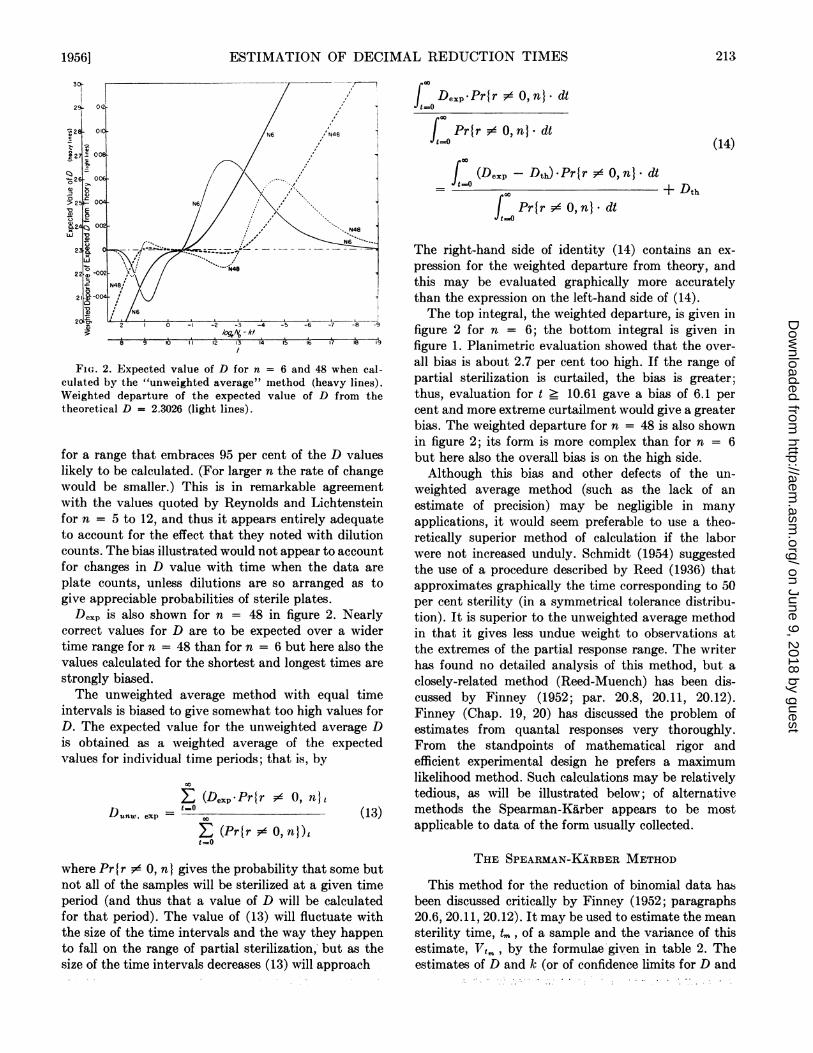
FIG. 1. Probability distribution curves for r = 0 to r = 6sterile samples in groups of six, where the probability P ofan individual sample being sterile is given by

log(- loge P) = loge No- kt, No ei k = 1.

and if e-kt is small, as it is when No is large comparedto N (by (1)),

loge P = -Noe-kt (9)

which is the approximation obtained by substituting- e-kt for x in the first term of the well-known series

2 3

log-(1+ x) = x - 2 + - < x < 1. (10)2 3

Ordinarily only the first term will be significant; aborderline example will be illustrated later (in footnote1 of Table 6). From (9) and (1)

p = e-Noe8kt -N

P=e =~-e (11Inasmuch as p = r/n is an estimate of P

= loge (n/r)

which is equation (3). Furthermore P = e- is theterm of the Poisson probability distribution for zerooccurrences where N is the expected or mean numberof occurrences (surviving organisms).The probability of obtaining r sterile samples in a

group of size n, is given by the general term of thebinomial probability distribution,

Pr{r} = pr(l _ p)n-r (12)r!(n - r

It is apparent that Pr {ri}, the probability of obtain-ing a particular value of r, will depend on ri, n, andthrough (11) on No, t, and k or D.

DEMONSTRATION OF BIAS IN THE UNWEIGHTEDAVERAGE METHOD

As an arbitrary example to illustrate the bias onemay take loge No = 10 (that is, No = e'° = 22,070)and k = 1 (that is, D = 2.3026). Variations in k in-volve only the units of the time scale, and variations

TABLE 1. Possible values of D of t = 13.20, NO = 00,k = 1, n = 6 (P = 0.96), and the weighted average

or expected value, De,pPr(rl Dr Prtrl -Dr

0.0000 0.00000.0011 2.932 0.00320.0204 2.787 0.05690.1957 2.597 0.5082

0.2172 0.5683

n-I

x(Pr r =- 0 = 2.616

Dep= n-I 0.21723 PrIrIr-1

* Calculated by (4).

in No (except to small values) involve only the dis-placement of the critical range of sterilization on thetime scale (figure 1). One might calculate P for variousvalues of t by (11) as a preliminary to calculatingPr{rJ by (12). More conveniently, one may take arbi-trary values of P and calculate the correspondingvalues of t and Pr{ r}. Tables of the latter have beenpublished (National Bureau of Standards, 1950;Harvard Computation Laboratory, 1955). The resultsof such a series of calculations for n = 6 are shown infigure 1. The asymmetrical character of all of thecurves may be noted.

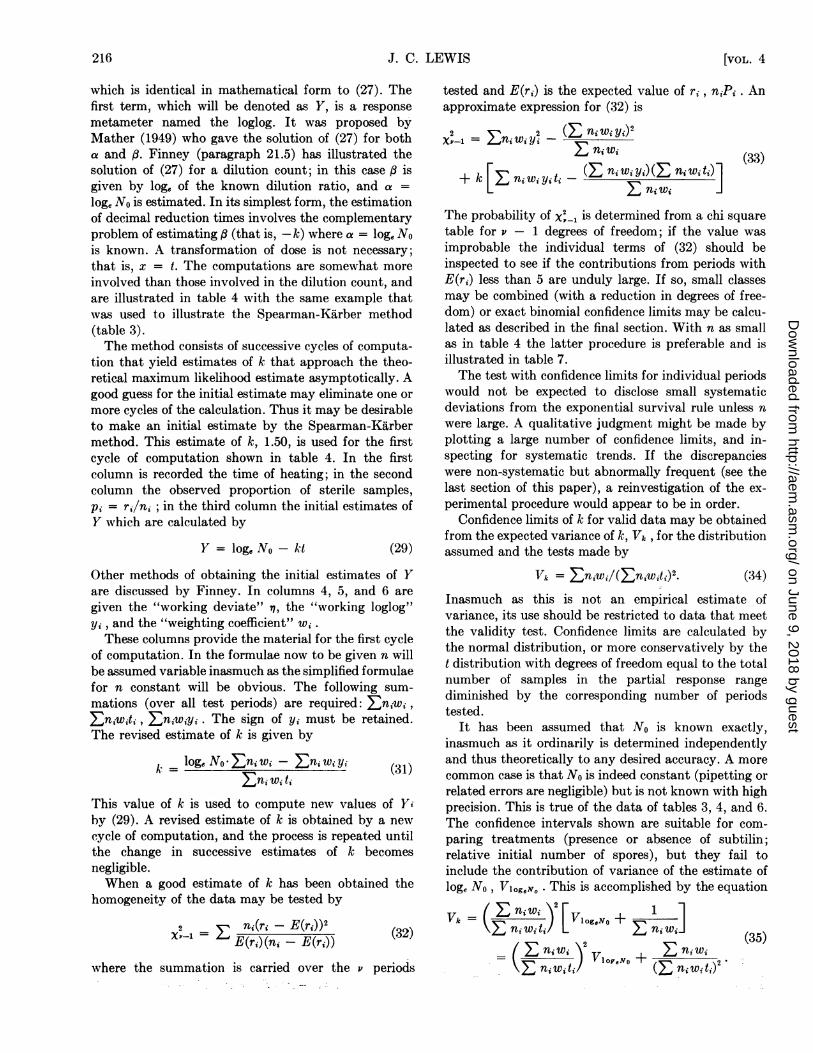
Consider the period t = 13.20. The probabilities ofobtaining 5 or 4 sterile tubes are appreciable; of ob-taining 3, 2, 1, or 0 are vanishingly small. The prob-ability of obtaining 6 sterile tubes is large, and if thishappens a value for D is not calculated. The expectedvalue for D, if one is calculated, is obtained asa weighted average as is illustrated in table 1. Valuesobtained in this way are plotted to give the expectedvalue of D as a function of the time of heating (figure2). For short periods of heating Dexp is less than thetheoretical D, Dth; for long periods Dexp is greaterthan Dth. Clearly this arises from rejecting observa-tions in which r = 0 or r = n. For short periods therejected observations are mostly r = 0; for long periods,mostly r = n.Because of the asymmetry of the curves of figure 1,

the 50 per cent sterility time (P = 0.50; t = 10 -loge (-loge 0.5) = 10.367) does not give an expectedD that is equal to Dth, 2.3026; instead Dexp = 2.298by the method of table 1, or 0.2 per cent lower than2.3026. By successive approximations, the time givingDexp = 2.3026 was found to be 10.610 (P = 0.581)for n = 6. The further t is from this time the greateris the departure of the expected D from the Dth . Forn = 6 the rate of change of Dexp with time approaches0.2 per minute, or 8.7 per cent of the theoretical value,and is approximately 0.12 (or 5.2 per cent) per minute

212 [VOL. 4

on June 9, 2018 by guesthttp://aem

.asm.org/

Dow

nloaded from

ESTIMATION OF DECIMAL REDUCTION TIMES

9/o0N - k28 9 c 12 13 14

t

Fi(. 2. Expected value of D for n

culated by the "unweighted average"Weighted departure of the expectedtheoretical D = 2.3026 (light lines).

= 6 and 48 when cal-method (heavy lines).value of D from the

for a range that embraces 95 per cent of the D valueslikely to be calculated. (For larger n the rate of changewould be smaller.) This is in remarkable agreementwith the values quoted by Reynolds and Lichtensteinfor n = 5 to 12, and thus it appears entirely adequateto account for the effect that they noted with dilutioncounts. The bias illustrated would not appear to accountfor changes in D value with time when the data are

plate counts, unless dilutions are so arranged as togive appreciable probabilities of sterile plates.

D0xp is also shown for n = 48 in figure 2. Nearlycorrect values for D are to be expected over a widertime range for n = 48 than for n = 6 but here also thevalues calculated for the shortest and longest times are

strongly biased.The unweighted average method with equal time

intervals is biased to give somewhat too high values forD. The expected value for the unweighted average Dis obtained as a weighted average of the expectedvalues for individual time periods; that is, by

2 (Dexp.PrIr - 0, itDunw exp = o (13)

E (Pr{r 0,n})nt=0

where Pr{ r 0, n} gives the probability that some butnot all of the samples will be sterilized at a given timeperiod (and thus that a value of D will be calculatedfor that period). The value of (13) will fluctuate withthe size of the time intervals and the way they happento fall on the range of partial sterilization; but as thesize of the time intervals decreases (13) will approach

fDexp.Prlr $O,n}. dt

f Prtr $ O,n). dt

IGoo

_ (Dexp -Dth) Pr{r $ O,n} * dt

f Pr{r $ O, n} * dt

(14)

+ Dth

The right-hand side of identity (14) contains an ex-pression for the weighted departure from theory, andthis may be evaluated graphically more accuratelythan the expression on the left-hand side of (14).The top integral, the weighted departure, is given in

figure 2 for n = 6; the bottom integral is given infigure 1. Planimetric evaluation showed that the over-all bias is about 2.7 per cent too high. If the range ofpartial sterilization is curtailed, the bias is greater;thus, evaluation for t _ 10.61 gave a bias of 6.1 percent and more extreme curtailment would give a greaterbias. The weighted departure for n = 48 is also shownin figure 2; its form is more complex than for n = 6but here also the overall bias is on the high side.Although this bias and other defects of the un-

weighted average method (such as the lack of anestimate of precision) may be negligible in manyapplications, it would seem preferable to use a theo-retically superior method of calculation if the laborwere not increased unduly. Schmidt (1954) suggestedthe use of a procedure described by Reed (1936) thatapproximates graphically the time corresponding to 50per cent sterility (in a symmetrical tolerance distribu-tion). It is superior to the unweighted average methodin that it gives less undue weight to observations atthe extremes of the partial response range. The writerhas found no detailed analysis of this method, but aclosely-related method (Reed-Muench) has been dis-cussed by Finney (1952; par. 20.8, 20.11, 20.12).Finney (Chap. 19, 20) has discussed the problem ofestimates from quantal responses very thoroughly.From the standpoints of mathematical rigor andefficient experimental design he prefers a maximumlikelihood method. Such calculations may be relativelytedious, as will be illustrated below; of alternativemethods the Spearman-Karber appears to be mostapplicable to data of the form usually collected.

THE SPEARMAN-KXRBER METHOD

This method for the reduction of binomial data hasbeen discussed critically by Finney (1952; paragraphs20.6, 20.11, 20.12). It may be used to estimate the meansterility time, t,, , of a sample and the variance of thisestimate, Vtm, by the formulae given in table 2. Theestimates of D and k (or of confidence limits for D and

1956] 213

on June 9, 2018 by guesthttp://aem

.asm.org/

Dow

nloaded from

J. C. LEWIS

TABLE 2. Formulae for the Spearman-Kdrber method;estimates of the mean sterility time, tm , and its

variance,* vimGeneral case:

tm 2 (4+1 + tiflr i r

vt^=~~ nj+nh1).( i(lPi-ti\ ti+ Pil/1-i

t;-l ti+l)2( ri(ni - ri)

Successive periods differ by equal time intervals, d:

d " rtm = tu + - - d Z -

2 i-..ni

V uP(P,( - Pi) U (ri(n,_-ri)

All periods involve an equal number of tests, n.

tm = 1 (ti+i+ t, (r,0 - ri)n \2 /

V,. 1- z I t-+ (P (1 -P))n ,..~ \ 2 /

Both d and n are constant:d d u

tm = tu + - --, r2 n i-l

(15)

TABLE 3. Estimation of survival rate constant k (ordecimal reduction time D) by the Spearman-

Kdrber methodSpores of Clostridium sp. PA 3679 in pea puree, No =

2.64 X 104, 120.1C., d = 0.5 minute throughout(data of O'Brien et al., 1956)

ti

(16)

(17)

(18)

(19)

5.56.06.57.07.58.08.59.09.510.010.511.0

(20)

(21)

Vgm = - 3 (Pi(1- Pi)) = 2 (r,(n - r) (22)n,-l n'(n - 1)

Summations are carried out in theory over all time periods;in practice, terms beyond a certain time, tu , have no effect.In formulae that do not involve Pi, tu may be any periodbeyond all those that give one or more viable samples. Pi isthe theoretical probability of a sample being sterile at ti,

and pi = i is an estimate of Pi . Better estimates of Pi , forni

use with the exact equations for Vt., may be calculated by(28) by means of a table of loglogs (Finney, 1952, AppendixTable XVI-see the next section) and k estimated by equation(25).The 95 per cent confidence limits for tm are taken as

tm 1 1.96(V,m), (23)

from the normal probability distribution as an approximationfor the distribution of tm .

* The variance is the square of the standard deviation. Thegeneral formula is not given by Finney but it may be obtainedfrom (15) by a conventional procedure described by Wilson(1952, p. 272).

k) are obtained by substituting t, (or the confidencelimits for t,,,) in

D = 2.3026 tm _ 4,tlog, No + 0.61 logio No + 0.265

andk =

log, No + 0.1tm

An example of the calculation is given in table 3.

(24)

,- /I.rt/ ni1

0/51/61/62/65/65/64/55/55/55/56/65/58.5

t i-6.514 4

= _ _ _

6 5= 3.133

ri/ni-ri)/fni(ni- 1)

05/1805/1808/1805/1805/1804/100

00000

8.5

ti-56.528 4180 100

= 0.1955

Y = log.-No - kt(by (29))

1.931.180.43

-0.32-1.07-1.82-2.57-3.32-4.07-4.82-5.57-6.32

P=c=SY(by (28))

.001

.039

.215

.483

.710

.850

.926

.964

.983

.992

.996

.998m P(1- P)

ti-0 n

0.1309 0.79335X4 6X4

= 0.0396

By (17)

tm= 4,+-d d ri/ni2

= 8.5 + 0.25 - 0.5 X 3.133

= 7.183

And by (18)

V = d2Z (ri(ni - r )/n.(ni - 1))

= 0.25 X 0.1955

= 0.0489

Then

1.96s = 1.96(V)i = 1.96 X .221

= 0.434and

tm = 7.183 4- 0.434

By (24)

D 2.303 (7.183 + 0.434)10.181 + 0.61

- 1.53 with confidence limits 1.44 to 1.63

By (2) or (25)

k = 1.50 (95% CL 1.42 to 1.60).

In the preceding calculations t. was taken as 8.5; a highervalue would have given the identical results.

Alternatively V maybe calculated by (18) with Pi estimatedby (28); this gives V = 0.0396 and k = 1.42 to 1.59.

Formulae (24) and (25) are taken from (4) and (2)(25) with log, N = log. (-log, Pm) = 0.61 corresponding to

Pm = 0.58. This value for Pm was obtained by esti-mating the bias of the Spearman-Karber method for

214 [VOL. 4

on June 9, 2018 by guesthttp://aem

.asm.org/

Dow

nloaded from

ESTIMATION OF DECIMAL REDUCTION TIMES

TABLE 4. Maximum likelihood estimation of k afterloglog transformation of response (data as in

table 8)

ti ri/-vi1i Yi w

5.5 0/5 1.9 -0.15 2.05 0.047 (i.e.,} X 0.056)

6.0 1/6 1.2 1.09 0.11 0.4136.5 1/6 0.4 -0.17 0.57 0.6467.0 2/6 -0.3 -0.41 0.11 0.5007.5 5/6 -1.1 0.49 -1.59 0.2818.0 5/6 -1.8 -0.10 -1.70 0.152

8.5 4/5-2.6-1.86 -0.74 0.060 (i.e., X 0.072)5

9.0 5/5-3.3 1.02 -4.32 0.030 (i.e., X 0.036)

9,.5 5/5 -4.1 1.01 -5.11 0.014 (i.e., 6 X 0.016)

10.0 5/5 -4.8 1.00 -5.80 0.007 (i.e., 6 X 0.008)10.5 6/6 -5.6 1.00 -6.60 0.004

11.0 5/5 -6.3 1.00 -7.30 0.002 (i.e., 6 X 0.002)

Z, witi wiy wi =2.156= 14.806 = -0.467

By (29), Yi = loge No -kti = 10.18 - 1.50 ti . One decimalplace in Yi ordinarily suffices.

The working deviate q is obtained from Y, and Pi ='i

by interpolation in Finney's Appendix Table XVII by meansof formulae 21.60, 21.61, and 21.62, p. 577. The working loglogyi is obtained by

y Y=-i 7. (30)

The weighting coefficient wi is obtained from Yi by inter-polation in Finney's Appendix Table XVII. When ni is notconstant it is convenient to adjust wi to a common basis

by multiplying wi by - , as has been done in the table withn

n = 6, and using n in the equation for variance (34).By (31),

(log. No): w - w, ys2; witi

10.18 X 2.156 + 0.467= 1.514

14.806

This estimate may be assumed not to differ sufficiently fromthe Spearman-Karber estimate to warrant another cycle ofcalculation. If it were thought to differ sufficiently anothercycle of calculations starting with Yi = 10.18 - 1.514 ti couldbe made, and in any event it would serve as a check on theprevious computation.

Conformity of the data to the binomial distribution shouldbe checked next. The number in each group, ni , is too smallto make the chi square test, (32) or (33), appropriate. A testby means of confidence limits for Y is illustrated in the firstparagraph of the last section of this paper. None of the con-fidence limits for k estimated in this manner for the individualtime periods are inconsistent with the loglog estimate of k;thus, there is no evidence of nonconformance to the binomialdistribution. The test can be made very rapidly inasmuch asit need be applied only to the most suspected periods; forexample, t = 6.0 and 8.5 in this table.

TABLE 4.-ContinuedAssuming No is known exactly, the theoretical variance

for k, by (34), is

Vk= =;w .50.00164.n(= uW ti)2 - 6(14.806)2

The 95% confidence limits are given by

k + 1.96 Vi = 1.52 4 0.08 = 1.44 to 1.60.

The significance of this estimate is discussed in the text, andincorporation of the variance of log, No is illustrated in thefirst footnote to table 6.

the limiting case of infinitesimally small equally spacedtime periods and the data of figure 1. Equation (17)then becomes

tm = tu - P dt.t=0

(26)

Planimetry of the integral, shown in figure 1, gave 4,, =10.61 and thus Pm = 0.58 by (11).

It is preferable that successive time periods be fairlyclose together, that the number of samples at eachperiod and the intervals between successive periods beconstant, and that the range of partial sterilization bebracketed completely. The requirement for a con-siderable number of test periods throughout the partialsterilization range implies that many tests will be madeat times that do not yield the most information. If theresponse range can be predicted well, the maximumlikelihood (loglog) method described below may allowenough saving in experimentation to compensate forthe more laborious computations.

MAXIMUM LIKELIHOOD ESTIMATION OF k AFTERLOGLOG TRANSFORMATION OF RESPONSE (THE

LOGLOG METHOD)Finney has discussed the general problem of com-

puting biological assays by estimating the parametersof "tolerance distributions," whether real or assumedbecause of the usefulness of the mathematical form,through transformations to provide a linear dependenceof a function of the response on a function of the dose.Thus

Y = a±+ox (27)

where Y is the transformed response (the "responsemetameter"), x is the transformed dose, (8 is theparameter of the tolerance distribution that is de-termined by the units of the dose scale, and a is theparameter that is determined by the position of thepartial response range on the dose scale.The tolerance distribution of samples of micro-

organisms that follow exponential survival whenexposed to heat is given by (11) which may be writtenas

log. (-log. P) = log. No- kt (28)

1956] 215

on June 9, 2018 by guesthttp://aem

.asm.org/

Dow

nloaded from

J. C. LEWIS

which is identical in mathematical form to (27). Thefirst term, which will be denoted as Y, is a responsemetameter named the loglog. It was proposed byMather (1949) who gave the solution of (27) for botha and Il. Finney (paragraph 21.5) has illustrated thesolution of (27) for a dilution count; in this case ,B isgiven by loge of the known dilution ratio, and a =

loge No is estimated. In its simplest form, the estimationof decimal reduction times involves the complementaryproblem of estimating # (that is, - k) where a = loge Nois known. A transformation of dose is not necessary;that is, x = t. The computations are somewhat moreinvolved than those involved in the dilution count, andare illustrated in table 4 with the same example thatwas used to illustrate the Spearman-Kairber method(table 3).The method consists of successive cycles of computa-

tion that yield estimates of k that approach the theo-retical maximum likelihood estimate asymptotically. Agood guess for the initial estimate may eliminate one ormore cycles of the calculation. Thus it may be desirableto make an initial estimate by the Spearman-Karbermethod. This estimate of k, 1.50, is used for the firstcycle of computation shown in table 4. In the firstcolumn is recorded the time of heating; in the secondcolumn the observed proportion of sterile samples,Pi = ri/n ; in the third column the initial estimates ofY which are calculated by

Y = log, No - kt (29)

Other methods of obtaining the initial estimates of Yare discussed by Finney. In columns 4, 5, and 6 aregiven the "working deviate" q, the "working loglog"yi, and the "weighting coefficient" w1.

These columns provide the material for the first cycleof computation. In the formulae now to be given n willbe assumed variable inasmuch as the simplified formulaefor n constant will be obvious. The following sum-mations (over all test periods) are required: Eniwi,EnXwiti, Eniwiyi. The sign of yi must be retained.The revised estimate of k is given by

k - log, No Enjwi- Eni wiyi (31)Eni wi ti

This value of k is used to compute new values of Yiby (29). A revised estimate of k is obtained by a newcycle of computation, and the process is repeated untilthe change in successive estimates of k becomesnegligible.When a good estimate of k has been obtained the

homogeneity of the data may be tested by

2 E 7ni(ri-E(rX2X1- = E(ri)(ni - E(ri)) (32)

where the summation is carried over the v periods

tested and E(ri) is the expected value of ri, n2Pi . Anapproximate expression for (32) is

X2-l = fliWi E-_(ni Wi yi)E niWi

+ k [ niiyi ti ( niwiyi)( niwiti)]~~~~Eniwi(33)

The probability of x'-, is determined from a chi squaretable for v - 1 degrees of freedom; if the value wasimprobable the individual terms of (32) should beinspected to see if the contributions from periods withE(ri) less than 5 are unduly large. If so, small classesmay be combined (with a reduction in degrees of free-dom) or exact binomial confidence limits may be calcu-lated as described in the final section. With n as smallas in table 4 the latter procedure is preferable and isillustrated in table 7.The test with confidence limits for individual periods

would not be expected to disclose small systematicdeviations from the exponential survival rule unless nwere large. A qualitative judgment might be made byplotting a large number of confidence limits, and in-specting for systematic trends. If the discrepancieswere non-systematic but abnormally frequent (see thelast section of this paper), a reinvestigation of the ex-perimental procedure would appear to be in order.

Confidence limits of k for valid data may be obtainedfrom the expected variance of k, Vk, for the distributionassumed and the tests made by

Vk = Eniwi/(Zniwiti)2. (34)

Inasmuch as this is not an empirical estimate ofvariance, its use should be restricted to data that meetthe validity test. Confidence limits are calculated bythe normal distribution, or more conservatively by thet distribution with degrees of freedom equal to the totalnumber of samples in the partial response rangediminished by the corresponding number of periodstested.

It has been assumed that No is known exactly,inasmuch as it ordinarily is determined independentlyand thus theoretically to any desired accuracy. A morecommon case is that No is indeed constant (pipetting orrelated errors are negligible) but is not known with highprecision. This is true of the data of tables 3, 4, and 6.The confidence intervals shown are suitable for com-paring treatments (presence or absence of subtilin;relative initial number of spores), but they fail toinclude the contribution of variance of the estimate ofloge No, Vlog6N0 . This is accomplished by the equation

Vk = (nw) [Vlog,,No + E (35)

=E(ni nwi 2 E niW i(35

*\E r Witi! (SV1OVNO+ 2tD

216 [VOL. 4

on June 9, 2018 by guesthttp://aem

.asm.org/

Dow

nloaded from

ESTIMATION OF DECIMAL REDUCTION TIMES

If both k and loge No must be estimated from thebinomial data (see Mather, 1949) the precision of theestimates will be greatly reduced.The loglog method of estimation of k with a single

time period gives a result identical with that given bythe unweighted average method. Thus k is obtaineddirectly from (31) by setting

y = Y = loglog p = loge loge (n/r). (36)

(Finney's Appendix Table XVI and National Bureauof Standards 1953, table 2, give this function.) Then

k loge No- y logeN0 - loge loge(n/r) (37)t t

which may be obtained by combining equations (4)and (2) of the unweighted average method. Thevariance for the loglog estimate, which would be equallyappropriate for the single period of the unweightedaverage method, is

Vk -2 (38)nwt2

It may be seen (by Finney's Appendix Table XVII or

in the figure given by Mather) that (38) will be minimalfor p equal to 0.20 approximately; that is, the estimatewill be most precise for this proportion of sterilesamples. It is the essential distinction between the twomethods that varying reliability of the data is takeninto account in the loglog calculation but not in the un-

weighted average calculation.Thus it becomes clear why use of the loglog method

can lead to far more efficient experimentation if the out-come can be predicted fairly well. Suppose that all ofthe tubes for the data of table 3 (and 4) had beenutilized at the period t = 6.5. The variance of theestimate of k would have been approximately

Eniw. = 6 X 2.16 =E nw 66 X 0.65

as great; that is, the confidence interval would havebeen less than six-tenths as wide. Put another way, theomission of periods t = 8.5 and longer would not havereduced the accuracy of the result appreciably. Theadvantage of reducing the number of dose levels inspeeding the computations will also be noted.Data that show a sharp cutoff have not been reducible

satisfactorily by the unweighted average method butthey present no problem to the loglog method. Considerthe arbitrary example shown in table 5. The data forcases I and II have been chosen as reasonably comingfrom the same population with the respective guessesof appropriate time periods. Not only are the resultsequally, readily, calculable but their reliabilities are

virtually identical.Similarly, data from curtailed response ranges offer

no difficulties for the loglog method. Such data give

biases in the unweighted average method, and theireffect on the Spearman-Karber method is not known.A more complicated situation arises where negative

exponential survival is not observed; that is, whereequation (1) does not hold. A common type of de-parture, illustrated by a sagging curve rather than a

Nlinear relationship of loge No vs. time, is given by a

population mixed with respect to resistance (k (or D)variable). This phenomenon has been discussed byRahn (1945, p. 19). It is demonstrated in a figure givenby O'Brien et al. (1956) for heat killing of Clostridiumsp. PA 3679 with various initial numbers of spores.Part of the original data have been treated by the vari-ous methods discussed in this paper with the resultsshown in table 6.Where exponential survival holds (the "controls" of

table 6) the agreement of the three methods is veryclose. Where exponential survival does not hold("subtilin present" of table 6) the agreement is verypoor for the lowest initial spore number. The confidencelimits calculated in the various ways shown also agreewell except with subtilin and the lowest initial sporenumber. Exact confidence limits for k calculated fromthe binomial probabilities (as outlined in the nextsection) for individual time periods agreed within the 5per cent level with the confidence limits shown in table6 in all cases.The overlapping of the confidence ranges of k for

various No in the controls and the failure to overlap inthe presence of subtilin demonstrates a departure fromexponential survival in the latter case but fails todemonstrate a departure in the former case.

It does not appear to be possible to make a sensitivetest for conformance to exponential survival by anymathematical device when only one inoculum level

TABLE 5. Loglog transformation for data with a sharpcutoff (arbitrary example; loge No = 5; n = 6)

r

Case I Case II

5 06 07 08 09 310 611 612 613 614 615 6

Case I: k = 0.599 Jh 0.080Case II: k -0.594 ± 0.079Combined data: k = 0. 0.597 4 0.057(95% confidence intervals)

19561 217

on June 9, 2018 by guesthttp://aem

.asm.org/

Dow

nloaded from

J. C. LEWIS

TABLE 6. Comparison of methods for calculating survival rate constants (extension of the data of tables S and 4)

Estimations of k with 95% Confidence IntervalsInitial Number of Spores Original Datat(No)* Unweighted SpamnKrbrLgo

averaget Spearran-Kirber Loglog

Controls2.64 X 101 0.5 (by 0.5) to 6 1.24 1.33 1.28

0, 0, 0, 0, 2, 5, 4, 6, 6, 5, 6, 6 (1.18-1.53)§ (1.09-1.47)6

(1.17-1.55)¶

2.64 X 103 3.5 (by 0.5) to 9 1.46 1.43 1.43

0, 0, 1, 0, 0, 3, 6, 5, 6, 6, 5, 5 (1.35-1.51)§ (1.34-1.52)6 5 6 5

(1.34-1.53)¶

2.64 X 106 5.5 (by 0.5) to 11 1.49 1.50 1.52

0, 1, 1, 2, 5, 5, 4, 5, 5, 5, 6, 5 (1.42-1.60)§ (1.44-1.60)5 6 5 6 5

(1.42-1.59)¶

Subtilin present2.64 X 101 0.4 (by 0.2) to 2.6 5.31 5.82 6.04

1, 4, 3, 6, 5, 6, 6, 6, 6, 6, 6, 6 4.75-7.54)§ (4.84-7.24)6

(4.92-7.14)¶

2.64 X 10 1.8 (by 0.2) to 4 3.12 3.09 3.18

0, 1, 1, 0, 3, 3, 4, 4, 5, 5, 6, 5 (2.88-3.33)§ (2.98-3.38)5 6 5 6 5 6 5

(2.92-3.29)1¶

2.64 X 104 2.8 (by 0.2) to 5 2.97 2.99 3.05

1, 0, 2, 1,3, 3, 5, 6, 5, 6, 6, 6 (2.83-3.16)§ (2.90-3.20)5 6 4 6

(2.86-3.13)T* For comparison of estimation methods and experimental treatments in this table, No has been assumed known exactly from

independent determinations. If absolute values for the confidence intervals were desired it would be necessary to introduce thevariance of log. No by (35). With low No the Poisson variance of No (which is equal to No) for equal volumes of the sample be-comes important for relative values of confidence intervals such as have been calculated here. Inserting the Poisson component

of variance of loge No, N in (35) gives

Iniw1 2t 1 1Vk =Kniwi4) (N + n ) (39)

For N = 26.4 in the control group

/15.2 2Vk =ji-)(0.038 + 0.066)

(40.5)which gives a confidence interval of :1:0.24 instead of the 40.19 shown in the table. The effect is much less marked in the othercases.

The accuracy of the approximation involved in equation (9) may be considered here. Retention of the second term of the ap-proximation; that is,

log. P =-No (ekl +

and calculation of the Spearman-KaLrber estimates of k with No = 26.4 gave values that differed from those shown in the tableby less than 0.5%.

218 [VOL. 4

on June 9, 2018 by guesthttp://aem

.asm.org/

Dow

nloaded from

ESTIMATION OF DECIMAL REDUCTION TIMES

TABLE 6.-Continuedt Note that the third code given below expresses the data given in table 3.

2.30261 By k = f: where bu.. is computed by (4) and (5). More simply, byfunwo

i41 clog. No-log, log.I )

§ Calculated as described in table 3, using ri and ni in (18).¶ Calculated as described in table 3, using (18) with Pi estimated by (28).

(40)

(No) is available. By far the best procedure is the use ofwidely-separated values of loge No .

CONFIDENCE LIMITS FOR BINOMIALLYDISTRIBUTED DATA

It is sometimes necessary to check in detail the basicassumption of a binomial distribution as well as theconformance to an assumed relationship of P to t. Fortests of exponential survival it is convenient to have theconfidence limits of Y = loge (- loge P) rather thanthe confidence limits of P. These are given for n < 16,a = 0.05 and 0.01, in table 7. An example of their usefollows: From the data of table 6, take the case ofNo = 2.64 X 103, subtilin present, t = 2 minutes,r/n = 6 (that is, one of six samples was sterile). Is thisresult consistent with the estimations of k shown intable 6? The confidence limits for Y, a = 0.05, are1.56, -0.61. Rewriting equation (29)

k loge No- Y (46)t

where j indicates one of the confidence limits. Then

7.88 - 1.56k____=_ = 3.16

2

7.88 + 0 _61+0.61=4.242

Similarly for a = 0.01

ki = 3.02, k2 = 4.46

By comparison with the confidence intervals of table 6it is seen that an estimation from this portion of thedata, representing a relatively short time of heating,does not depart from the estimations from all the datawith significance even at 5 per cent.

Confidence intervals have been calculated for thedata of Pflug and Esselen (1954), for which n = 48,because the bias in the unweighted average method ofcalculation that they used is inadequate to account forthe deviations that they found from predictions basedon exponentially decreasing survival. The nature of thediscrepancies become more clear if the probability thatan individual spore survives is plotted on a logarithmicscale against time of heating on a linear scale. This

probability, H, is given by the ratio of the final to theoriginal number of spores; by (1) and (9)

log. II = log. (N/No)= -kt = log. (-log. P) - log. No

= Y - loge No.

(47)

By substituting the confidence limits for Y in (47) the99 per cent confidence intervals for loge H shown asvertical bars in figure 3 were obtained. Those thatcorrespond to ri = 0 or ni are unbounded on top orbottom. The diagonal lines through log., H = 0 givepredicted values of log, II for loglog estimates of k.As Pflug and Esselen point out, the data deviate

markedly from expectation for exponential survival. Itis more pertinent, however, that the data also deviatemarkedly from expectation for a binomial distribution.Three discrepancies will be detailed. One may firstconsider the confidence intervals marked A correspond-ing to the times 0.0562 and 0.0599 and No = 120. Noreasonable course for log. II could pass near both ofthese intervals. On the reasonable assumption thatlog. II = -90.65t in this local region the probabilityof obtaining a value of r as low as that observed (0) att = 0.0562 and a value as high as that observed (45) att - 0.0569 would be infinitesimal, much less than 10s4.As a matter of fact, no reasonable course for log, Hcan be drawn through either one of these confidencelimits and the others for No = 120.Even more marked discrepancies are apparent

between sets of data for the various initial numbers.Attention is directed to the regions B and C that arebounded roughly by dotted lines. Region B has at least10 confidence intervals that are inconsistent with anyreasonable single-valued function for log. H; region Chas at least 7. If it be assumed that the initial concen-tration of spores was not known, marked changes in thedilution ratios (that is, to less than A instead ofibetween No = 120 and No = 104) would have to beassumed to reconcile region B.

It perhaps is idle to speculate further as to thenature of the extraneous factors that have given theseanomalous data; they point up the need for statisticalcontrol even with an experimental setup as apparently

2191956]

on June 9, 2018 by guesthttp://aem

.asm.org/

Dow

nloaded from

0) -4 eq em 1d Co5 co t- CC CC1 0 -. eq C) "4' Co Co

Lo@0@ @0 @0 @ @00 so- .4-0 e- 40 eC4 V- 8-

II . C C C - C - ~~~~ ~~ ~~ ~~~~~~C-C; Ci C - - C - C - C - C; C- C -

ae CD (4 tq 10-m@0 @o @o @o @o @0 .40 -- C~~~~~~~~~~~~.4.---0 lo- "II aCOq ".,to o 88 CM-4C01 10 a'ID-i II I, VIIC II II- II II Ico I II

Vi CiC~ 'I 119 ! 09 i Iq C OOl 0. .4 c q C C

50C cci- CC'(-- C 50CC 0- 94Ot- COO (4 '4L-o

@0 @0 0@0 @09 .4 C-V 4-4 cq cq 884,

eeq C4 P5C4 t so 0 MWe1a CC lo co

() @0 @00C)0C @0 v-o V.o-4 4- 4-- gi s#40 COOv; e(-C:8

V4-~.. - @ 0 @0 @0 @0a @0 @0 0Ca @0-@

@-40 @0 @0 @0 V44o .- .-4- socq e .. rs 88

II -0 0CC~~~44-4 CO 00 C (-C 5C 0 -- - -

"W sm gm~OC~0 CC) COO 5CC t

!I -Ci 150CC IC.4CC 09C- *C CC -C I

8o8 C>- Co @0 @0 @0 @0@40@0@0M

vo 0 @0 w40 s i- # eq u 8

II 5CC PC~ s-C .~IRC - - - -I2 OCo 04 ~~~~~~~4-~ 2CC 31 94 C ¶ o34

o c 3o- COC(-4 CC C CO- C00~ ~ ~ ro 501 tC s1~

@0 @0 C1@0 o-M s-- #14- tic- V4C 48t 8co M- aC r s-CC (01 @ 0V4C1 -

-. 4 :4 *iC : 0 CC COO COCo! 09Ci 'IR 0.4CC.: 50C C

88 s-~~~~~ -- ~~~~~o @0~c teo @0-

2 ~ ~ ~ ~ ~ ~ ~ ~C.I l! C

V-(C4C 0 OO

@0 @40 C4o- s-i ti c- c 8

II II II II IIC II I C

CiC 4 CO . rCo C

II~~~~~~9Ri -

w43C) Co 0C) 0C

tl~ ~ ~ o O C!- #4' S

@40 s-O #4 COl48

v-4~ ~ ~ II C

II - . - C

24 II

WCOO

80

CO

0

CO

0

0

2

2CO

0

0*0CO08

.002

0

.02

iC..*C)

COC.OCO20

'!C0

.Ieq.v1I VII -.

.MVII..AJISC ..

*0COO.COC0 .

.II.eq .

Vii . .

VII 01SC SC

C CC

2 0CC

2 CO0.0

2 22

02.0CO20

2 0122 SCC SCOC 0C CCCCO

-CC

2 20

.C 05CC

C 82CO

2 CCC.

20

2'

022

C 2

.COC CCCCO .C. COC,-. 2

CO~CO1 CO'- 8:8>~g . 4~

00

+2 )

VCO 01

V C,1~ ~~ C

0.-l0

2.4

00

2 OZC

2 S.C2 0

2CD

Vil Q10 4.

;3 0"I' 0 2

1.- 'a. gt 419 -.0C.) .r -.z 00f.)as M dC.)al 2 J.,- ask a "

to0 4) 0.q 0;Z4 M 00

220

0

H

2-.0

CC)SC)

-0

CO02-.

0

CO

CC)

SC).

.OC

0

SC) IICC)

.0

I:2C4.CC

2)

02).0

0

.. 0)

* .

CCCbC

.CC 2)

CCCoCC).C

SC) b12.2)

0

Co.

t,- 0II

Ci

.'CCC.

H-2)2)

2)02)

00

0202Co2)

2)0

-e0

on June 9, 2018 by guesthttp://aem

.asm.org/

Dow

nloaded from

ESTIMATION OF DECIMAL REDUCTION TIMES

simple as this onie. Certainily the data cannot be con-sidered to demonstrate a trend in D values calculatedby the unweighted average method that is greater thanthe inherent bias in this method.

It must be emphasized that the anomalies in thePflug and Esselen data are striking because fairly largenumbers of tests were run. These authors correctlypoint out that large numbers are required for narrowconfidence limits; they appear to assume that largenumbers guarantee high confidence. There is no reasonto assume that other experiments of this type done withfewer numbers are not subject to similar disturbances,in the absence of a demonstration of statistical control.The many pertinent biological factors are beyond thescope of this discussion.

ACKNOWLEDGMENTThe writer is indebted to Dr. T. A. Jeeves, formerly

of the Statistics Laboratory, University of California,for discussions of confidence limits for the binomialprobability distribution and for suggesting the methodof presentation of figure 3.

SUMMARYIn connectioin with the estimationi of deciimal re-

duction times (D values) for populations that decreaseexponentially with time ("logarithmic order of death"),the calculation of D for individual times of heating frombinomial data (dilution endpoint counts) gives anapparent dependence of D on time of heating. It is

Time In Minutes

FIG. 3. Exact binomial confidence limits (99 per cent)

for the data for Pflug and Esselen (1954). The diagonal linesrepresent the loglog estimates of k.

demonstrated that the apparent dependence arisesfrom the bias obtained by rejecting observations whereall samples show growth (short periods of heating) andwhere no samples show growth (long periods of heating).Preferred methods of calculation (Spearman-Kiarberand loglog methods) are illustrated.

REFERENCES

BENNETT, C. A., AND FRANKLIN, N. L. 1954 StatisticalAnalysis in Chemistr-y and the Chemical Induistry. JohnWiley & Sons, Inc., New York.

FINNEY, I). J. 1952 Statistical Method in Biological .Assay.Hafner Puiblishing Company, New York.

HARVARD UNIVERSITY, STAFF OF THE COMPUTATION LABORA-TORY 1955 Tables of the Cumulative Binomial Prob-ability Distribuition. Harvard University Press, Cam-bridge, Mass.

MATHER, K. 1949 The analysis of extinction time data inbioassay. Biometrics, 5, 127-143.

NATIONAL BUREAU OF STANDARDS 1950 Tables of the Bi-nomial Probability Distribution. Applied MIathematicsSeries, 6. U. S. Government Printing Office, Washington,D. C.

NATIONAL BUREAU OF STANDARDS 1953 Probability Tablesfor the Analysis of Extreme-Value Data. Applied Mathe-maties Series, 22. U. S. Government Printing Office,Washington, D. C.

O'BRIEN, R. T., TITUS, 1). S., D)EVLIN, K. A., STUMBO, C. R.,AND LEWIS, J. C. 1956 Antibiotics in food preserva-tion. II. Further studies on the influence of subtilinand nisin on the thermal resistance of food spoilage bac-teria. Food Technol. (in press).

PFLUG, I. J., AND ESSELEN, W. B. 1954 Observations onthe thermal resistance of putrefactive anaerobe No. 3679spores in the temperature range of 250-300 F. FoodResearch, 19, 92-97.

RAHN, 0. 1945 Injury and Death of Bacteria by ChemicalAgents. Biodynamica monographs, Biodynamica, Nor-mandy, Missouri.

REED, L. J. 1936 Statistical treatment of biological prob-lems in irradiation. In Duggar, B. M., Editor, Bio-logical Effects of Radiation, Vol. 1, p. 243. McGraw-HillBook Co., New York.

REYNOLDS, H., AND LICHTENSTEIN, H. 1952 Evaluation ofheat resistance data for bacterial spores. Bacteriol.Revs., 16, 126-135.

SCHMIDT, C. F. 1954 Thermal resistance of microorganisms.In Reddisch, G. F., Editor, Antiseptics, Disinfectants,Fulngicides, and Chemical and Physical Sterilization, p.732. Lea and Febiger, Philadelphia.

STUMBO, C. R., MURPHY, J. R., AND COCHRAN, J. 1950 Na-tire of thermal death time curves of PA 3679 and Clostri-dium botulinutm. Food Technol., 4, 321-26.

THOMPSON, C. M. 1941 Tables of percentage points of theincomplete beta-function. Biometrika, 32, 151-181.

WILSON, E. B. 1952 An Introduction to Scientific Research.McGraw-Hill Book Co., New York.

1956] 221

on June 9, 2018 by guesthttp://aem

.asm.org/

Dow

nloaded from