r.f.h. roijmans model-based optimization of drilling fluid

R.F.H. Roijmans

Model-based optimization

of drilling fluid density and

viscosity

Tec

hnis

che

Univ

ersi

teit

Del

ft

Model-based optimization of

drilling fluid density and viscosity

By

Roel F.H. Roijmans

in partial fulfilment of the requirements for the degree of

Master of Science

in Applied Earth Sciences with specialization Petroleum Engineering

at the Delft University of Technology,

to be defended publicly on Wednesday July 6, 2016 at 14:00 PM.

Supervisor: Prof. Dr. Ir. J.D. Jansen Thesis committee: Dr. P. Astrid Shell

Dr. J.J. Blange Shell Dr. W. Broere TU Delft Prof. Dr. P.L.J. Zitha TU Delft

This thesis is confidential and cannot be made public until January 6, 2017.

An electronic version of this thesis is available at http://repository.tudelft.nl/.

The work in this thesis was supported by Shell Global Solutions. Their cooperation is hereby gratefully acknowledged.

Abstract

Optimization of drilling fluid properties is an essential part of cost effective drilling operations and process safety. Currently fluid properties are measured and optimized manually by human engineers with different skills and experience which might lead to non-optimum drilling fluid properties that deteriorate its functionalities. Automated drilling fluid management is still at an early development stage. Several vendors are actively developing automated skids to measure drilling fluid properties in real time [1] [2], and several authors also have published scientific work on the use of the real-time measurement as a component of automated control systems that dose mud additives automatically to meet the mud specifications or setpoints defined by human engineers [3] [4]. During the well planning stage, the design process of mud specifications is carried out by engineers checking several scenarios using well planning software and their experience to come up with drilling fluid specifications. When hole cleaning and/or borehole stability conditions change during the actual drilling process that warrant updates or changes of drilling fluid properties, the specifications are updated in an ad-hoc manner, relying on the skills of human engineers. This thesis focusses on the development of a model-based optimization module for drilling fluid properties to help engineers in the planning and drilling phase to automatically derive drilling fluid specifications that meet the hole cleaning criteria, and satisfy the downhole pressure requirement and constraints set on the operating ranges of drilling parameters. The optimization framework will use proxy models derived from well hydraulics software that predicts cuttings concentration and downhole pressure as a function of the drilling fluid properties. Three objective functions for the optimization module are given as examples in this thesis. The first two objective functions deal with the hole cleaning criteria while the last one is a cost function that combines the cost of hole cleaning and downhole pressure management. The optimization module has been tested on a case study based on real field data. Given an objective function, multiple constraints, and proxy models, the module takes only a few seconds to find the optimum mud property values and drilling parameters such as flow rates, rotary speed and rate of penetration. A benchmark with the field data shows that the optimum drilling fluid properties and parameters result in significant improvement of the hole cleaning state while the downhole pressure requirement and constraints on the drilling parameters can still be satisfied. When a cost function is defined as a combination of hole cleaning and downhole pressure management, the module also gives a quantified benefit of the trade-off between maximizing hole cleaning and minimizing losses. Since this module can perform optimization very efficiently compared to the ad-hoc processes done by human engineers, this module may be of significant value for operating units to use in the planning and drilling phase and also in the future as an outer optimization loop for automatic drilling fluid control systems.

Table of Contents

Abstract ......................................................................................................................................................... i 1 Introduction .............................................................................................................................................. 1

1.1 Research scope ............................................................................................................................................................. 3 1.1.1 Problem statement ............................................................................................................................................... 3 1.1.2 Research question statement .............................................................................................................................. 3 1.1.3 Thesis outline ........................................................................................................................................................ 4

2 Well hydraulics kernel .............................................................................................................................. 5

2.1 First principles of the hydraulics kernel .................................................................................................................... 5 2.1.1 Downhole pressure .............................................................................................................................................. 5 2.1.2 Cuttings concentration ........................................................................................................................................ 6 2.1.3 Output parameters of interest ............................................................................................................................ 7

2.2 Identification of parameters of interest .................................................................................................................... 8 2.3 Sensitivity analysis of kernel ....................................................................................................................................... 9 2.4 Conclusions................................................................................................................................................................... 9

3 Proxy model derivation ............................................................................................................................ 11

3.1 Observed data ............................................................................................................................................................. 12 3.1.1 Equivalent circulating density at the bit .......................................................................................................... 12 3.1.2 Worst hole cleaning index ................................................................................................................................. 12 3.1.3 Total hole cleaning index .................................................................................................................................. 13 3.1.4 The algorithms .................................................................................................................................................... 13

3.2 Linear regression model ............................................................................................................................................ 13 3.3 Stepwise regression .................................................................................................................................................... 14 3.4 Summary of proxy model derivation ...................................................................................................................... 15 3.5 Accuracy of proxy models ........................................................................................................................................ 15

3.5.1 Criteria for fitting accuracy ............................................................................................................................... 15 3.5.2 Criteria for predictive capability ....................................................................................................................... 17 3.5.3 Statistical criteria ................................................................................................................................................. 18

3.6 Methods to improve proxy model quality .............................................................................................................. 19 3.6.1 Skewing ................................................................................................................................................................ 20 3.6.2 Larger design ....................................................................................................................................................... 21 3.6.3 Discussion ........................................................................................................................................................... 22

3.7 Conclusions and recommendations ........................................................................................................................ 22 4 Optimization modules ............................................................................................................................ 23

4.1 Inputs for numerical optimization .......................................................................................................................... 24 4.2 Analysis of objective function .................................................................................................................................. 25 4.3 Test case study ............................................................................................................................................................ 26 4.4 Optimization check ................................................................................................................................................... 28 4.5 Conclusions and recommendations ........................................................................................................................ 28

iv

5 Case studies & Cost functions ............................................................................................................... 29

5.1 Case study I ................................................................................................................................................................. 29 5.2 Case study II ............................................................................................................................................................... 31

5.2.1 Optimizing for viscosity only ........................................................................................................................... 32 5.2.2 Adding three parameters ................................................................................................................................... 33 5.2.3 Conclusions ......................................................................................................................................................... 34

5.3 Cost functions ............................................................................................................................................................ 34 5.4 Conclusions and recommendations ........................................................................................................................ 38

6 Conclusions and recommendations ....................................................................................................... 39

6.1 Conclusions................................................................................................................................................................. 39 6.2 Recommendations ..................................................................................................................................................... 40

Appendices ................................................................................................................................................ 39 A Rheology ............................................................................................................................................................................ 41 B Input hydraulics software ................................................................................................................................................ 45 C Values of input parameters .............................................................................................................................................. 47 D Extended range sensitivity .............................................................................................................................................. 51 E Design of experiments ..................................................................................................................................................... 53 F The p-value ......................................................................................................................................................................... 57 G Amount of observed data ............................................................................................................................................... 59 H Skewing .............................................................................................................................................................................. 61 I Analytical description of optimization problem ............................................................................................................ 65 Bibliography .............................................................................................................................................. 67 Glossary ..................................................................................................................................................... 69

List of Symbols ................................................................................................................................................................. 69 List of Acronyms .............................................................................................................................................................. 69

Acknowledgements .................................................................................................................................... 71

Chapter 1

1Introduction

Drilling automation is an active area within the oil and gas industry, driven by the need to improve well construction quality, safety and cost efficiency. Examples of automated drilling tools include the rotary steerable system [5] [6] and automatic controllers to eliminate torsional drill string vibrations [7]. The drilling fluid or mud system is also a vital component of every drilling operation and accounts for about 10% of total well costs. Drilling fluid management is a critical component of process safety and cost effective drilling operations, however automated drilling fluid management is still at an early development stage compared to the automation of drilling mechanics aspects. Drilling fluid management currently relies for a large degree on manual operations [8]. The main objective of this thesis is to develop an automatic, model-based optimization framework that can be used as a part of a pre-drill planning activity or in real-time drilling fluid management.

Motivation

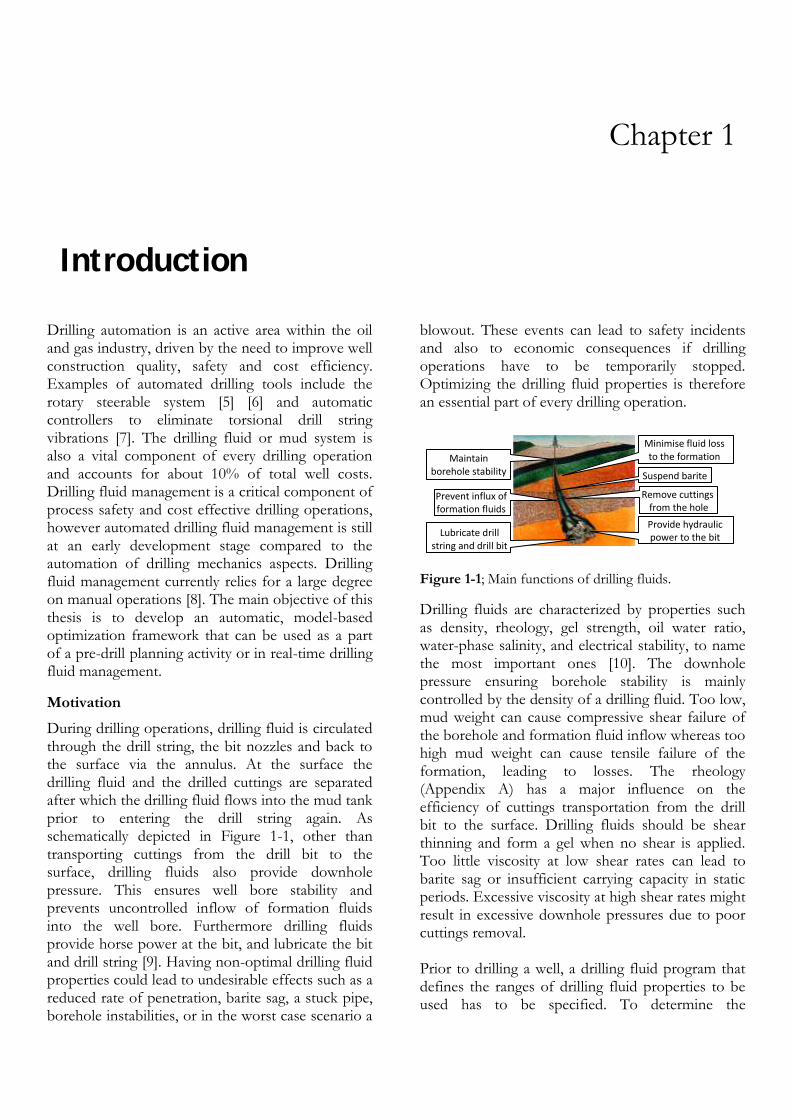
During drilling operations, drilling fluid is circulated through the drill string, the bit nozzles and back to the surface via the annulus. At the surface the drilling fluid and the drilled cuttings are separated after which the drilling fluid flows into the mud tank prior to entering the drill string again. As schematically depicted in Figure 1-1, other than transporting cuttings from the drill bit to the surface, drilling fluids also provide downhole pressure. This ensures well bore stability and prevents uncontrolled inflow of formation fluids into the well bore. Furthermore drilling fluids provide horse power at the bit, and lubricate the bit and drill string [9]. Having non-optimal drilling fluid properties could lead to undesirable effects such as a reduced rate of penetration, barite sag, a stuck pipe, borehole instabilities, or in the worst case scenario a

blowout. These events can lead to safety incidents and also to economic consequences if drilling operations have to be temporarily stopped. Optimizing the drilling fluid properties is therefore an essential part of every drilling operation.

Figure 1-1; Main functions of drilling fluids.

Drilling fluids are characterized by properties such as density, rheology, gel strength, oil water ratio, water-phase salinity, and electrical stability, to name the most important ones [10]. The downhole pressure ensuring borehole stability is mainly controlled by the density of a drilling fluid. Too low, mud weight can cause compressive shear failure of the borehole and formation fluid inflow whereas too high mud weight can cause tensile failure of the formation, leading to losses. The rheology (Appendix A) has a major influence on the efficiency of cuttings transportation from the drill bit to the surface. Drilling fluids should be shear thinning and form a gel when no shear is applied. Too little viscosity at low shear rates can lead to barite sag or insufficient carrying capacity in static periods. Excessive viscosity at high shear rates might result in excessive downhole pressures due to poor cuttings removal. Prior to drilling a well, a drilling fluid program that defines the ranges of drilling fluid properties to be used has to be specified. To determine the

Provide hydraulic power to the bit

Remove cuttings from the hole

Prevent influx of formation fluids

Maintain borehole stability

Lubricate drill string and drill bit

Minimise fluid loss to the formation

Suspend barite

2

appropriate ranges of drilling fluid properties, the cuttings concentration and pressure distribution along the entire wellbore are simulated using a well hydraulics software, or often referred to as the well hydraulics kernel. The cuttings concentration everywhere along the wellbore should be as low as possible and the simulated pressure distribution should fall within the expected fracture and pore pressure gradient. Those gradients are determined prior to the simulation by a borehole stability software [11]. This software uses knowledge gained from offset wells and data acquired with geological studies. The primary driver of this work is to automate and standardize the optimization process of drilling fluid properties, in order to improve hole cleaning and borehole stability during a well construction process. Currently, prior as well as during drilling, fluid properties are optimized manually by human engineers with different skills and experience which might lead to the implementation of non-optimal fluid properties. Other than drilling fluid properties, the well hydraulics kernel takes other operational parameters such as the drilling rate of penetration, rotary speed, and flow rate, and the wellbore geometry, and the measures of the drill string assembly as input parameters and outputs several indicators of hole cleaning along the wellbore such as cuttings bed height and concentration and the pressure distribution [12]. An engineer simulates various values of drilling fluid properties as proposed by A. Tutuncu et al [13] and J. Dudley et al [14]. Given these simulation scenarios, multiple curves for the cuttings concentration and for the pressure distribution are obtained. The drilling parameters and mud property values that produce the curve with the best hole cleaning while satisfying a pressure distribution that falls within the pore pressure and the fracture gradient, are considered as optimal parameters. These drilling fluid parameters are then proposed by the planning team to the well delivery team. Using this manual approach only a limited number of combinations can be tested because the kernel calculations take a lot of time due to the kernel its complex and non-linear nature. Finding the true optimal setpoints is therefore difficult.

While drilling the pore pressure and/or fracture gradient might be updated based on real-time data. Since the above described optimization procedure is a time consuming process, it cannot be repeated in a timely manner while drilling. Hence when relevant real-time data becomes available or when downhole conditions deviate from the expected pressure window, the drilling fluid properties are updated in an ad-hoc manner, largely based on the experience of an engineer. This lack of systematic and integrated drilling fluid management leads to costly events such as stuck pipe, drilling fluid losses that typically cost operations 2% to 4% of the total well cost to manage. The risk of hole cleaning and borehole stability events is very prominent in depleted reservoirs, where the window between the pore pressure and fracture gradient is narrow. The manual handling and measurement of mud properties also contributes to inefficiencies in drilling fluid management. In recent years, vendors have developed automated mud skids that can measure mud properties such as density and viscosity in real time [1] [2]. Real-time control concepts using real-time mud measurement data have also been demonstrated in the work of T. Schuit [3], L. van der Sluis [15], and R. Nafikov & S. Glomstad [4]. For implementation, these controllers have to be connected to an automated mixing system, an example of which is given in [16]. In the future, it is envisioned that the control loop and the real-time measurement data are connected to an outer model-based optimization loop that computes targets or setpoints of mud properties for the control systems automatically (Figure 1-2).

Figure 1-2; Closed loop control of mud properties, connected to an outer model-based optimization loop.

1.1 Research scope

Regulating the downhole pressure and transporting drilled cuttings are the most important functions of drilling fluids. These two functions are closely related to drilling fluid density and rheology, respectively. The focus of this thesis will therefore be on finding the optimal density and rheology properties to improve hole cleaning and maintain borehole stability.

1.1.1 Problem statement

The core challenge of this study is identified as: The drilling fluid properties resulting in optimal hole cleaning and borehole stability are currently determined manually instead of systematically. This challenge originates from the fact that the well hydraulics model is a black box to common users. The underlying first principle model of the well hydraulics kernel is a set of nonlinear partial differential equations that has to be solved numerically. One has to run multiple simulations and compare all outputs to decide on what one considers the optimal drilling fluid properties. In this study an automatic setpoint search algorithm is envisioned to systematically determine the optimal drilling fluid density and rheology that result in optimal hole cleaning at all times and simultaneously a downhole pressure between the pore pressure gradient and the fracture gradient. The problem statement can be summarized as

Here XJ is the overall objective function that can

be decomposed as:

Xii fJ Objective function i associated with

an output Xif of the kernel, for

example the hole cleaning index or the equivalent circulating density.

Xif Output i of interest of the well

hydraulics kernel such as hole cleaning index or equivalent circulating density, represented as unknown non-linear function of input variables of the kernel.

X Vector containing the values of all the kernel its input parameters.

U and L Superscripts denoting the upper and lower bound respectively.

1.1.2 Research question statement

The main research question for this study can now be formulated as: “Can a model-based optimization framework be used to find automatically optimal drilling fluid properties during the planning phase and potentially real-team drilling process and what improvements can be made with respect to the hole cleaning and borehole stability when the solution of this optimization framework is used instead of the drilling fluid properties once used in the field?” To investigate the feasibility of the proposed automatic setpoint search algorithm, four research objectives are set. The objectives are: 1. By using the hydraulics kernel, parametrize the

relationship between the outputs of the kernel

such as hole cleaning index and equivalent

circulating density and some of the input

parameters, denoted by the vector x, as xif .

These input parameters should include drilling

fluid density and viscosity, and this set might be

expanded as indicated in Objective 2.

2. Identify other operational input parameters that

have a significant influence on outputs of the

kernel.

3. Develop an optimization module which uses the

identified relationships xif , called proxy

General optimization framework

Maximize

XXXXX ni JJJJJ ......21

X

XXX

nn

ii

fJ

fJfJfJ

...

...2211

Subject to

XXXU

ii

L

i JJJ

XXXU

ii

L

i fff U

ii

L

i XXX

4

models, as objective functions and/or

constraints.

4. Test to automatic setpoint search algorithm on

several case studies based on real field data, and

quantify the improvements made.

By fulfilling those objectives we hope to show that

the optimal drilling fluid properties can be calculated

automatically in a more standardized and systematic

way as compared to current practice.

The workflow followed in this study is schematically

depicted in Figure 1-3. Firstly, a well hydraulics

kernel that predicts the down hole pressure and hole

cleaning should be available. Secondly, given the

advised parameter ranges of drilling fluid properties,

drilling parameter simulations following a systematic

experimental design procedure are run. Thirdly,

proxy models are derived to approximate the input-

output relationships given the simulation results.

Finally, numerical optimization techniques are used

to find the optimal drilling fluid properties given an

objective function, the proxy models, and

constraints.

Figure 1-3; The workflow of this study.

Throughout this thesis it will be assumed that the results generated by the hydraulics kernel are representing reality. That is, the responses as calculated by the kernel are in agreement with what one would measure in the field using a sensor. This thesis will not compare measured responses of sensors with responses as simulated by the hydraulics kernel in an attempt to validate or improve the hydraulics kernel [17].

1.1.3 Thesis outline

The structure of this thesis is as follows. In Chapter 2 the basic structure of the hydraulics kernel will be introduced. Then, together with previous work, a single dimensional sensitivity analysis will be the basis for deciding which parameters to include in the proxy models. In Chapter 3 the workflow of how to obtain a mathematical formulation for a proxy model is described in detail. Subsequent validation of a developed proxy model is done by checking its accuracy based on introduced and pre-set criteria. Chapter 4 focuses on finding the optimal drilling fluid properties. An optimization module will be developed containing an optimization algorithm and the developed proxy models as objection and/or constraint functions. Chapter 5 demonstrates the integrated work flow by discussing two case studies - one of them in relation with the input from borehole stability software. The improvements made when using setpoints as calculated by the developed algorithm instead of the setpoints actually used in the field are quantified. In an endeavour to value improvements made in hole cleaning and/or downhole pressure, lastly the concept of a cost function is introduced.

Hydraulics kernel

Suitable parameters & ranges

Proxy model

Optimal drilling fluid properties

ppp statictotal

gDp dfstatic

ccdfMDdf CTPD ,,,

Chapter 2

2Well hydraulics kernel

The goal of this work is to develop an optimization module with the objective of maximizing hole cleaning and/or minimizing pressure subject to hole cleaning, pressure, and other constraints. Shell has developed an in-house software, the Well Hydraulics kernel, which is a simulation tool for predicting the downhole pressure and various quantifications of hole cleaning capabilities. To simulate the downhole pressure and hole cleaning indicators as a function of depth, the kernel divides the spatial domain of the wellbore in O(103) grid cells and solves the Navier Stokes equation. The calculations performed by the kernel (typically one second per calculation) have been used by well engineers as a planning and real-time monitoring tool to optimize drilling parameters. In this chapter, the main principles of the hydraulics kernel will be introduced. Then a screening procedure is followed that selects which parameters might be of interest for the to-be-developed optimization module. In the last Section a sensitivity analysis is performed on the selected parameters.

2.1 First principles of the hydraulics kernel

The input data to the kernel covers both well design parameters as well as operational parameters. Well design parameters include among others the open hole diameter, the casing inner diameter, the true vertical depth and the measures of the drill string. Operational parameters include among others cuttings density, cuttings size, flow rate, rate of penetration and drilling fluid properties. An extended list of the input parameters, explaining 95% of the observed pressure variations [18], is

presented in Appendix B. The primary outputs of the kernel are pressure and cuttings concentration, both simulated as a function of depth. The kernel also calculates several quantities related to those two. These include the frictional and static pressure, the equivalent circulating density, the suspended cuttings concentration, the bed height, the open flow area, and the hole cleaning index. In the following two Sub-sections the first principle model of the downhole pressure and the cuttings concentration will be given.

2.1.1 Downhole pressure

A direct measure of the downhole pressure can be done by a pressure while drilling (PWD) sensor. These sensors are typically only installed as a part of a bottom hole assembly in high value wells due to their high cost, and those measurements are limited to a single sensor close to the bit. Therefore, it is useful to have a downhole pressure prediction tool. Analytically the downhole pressure is defined as

2-1

Here, the total pressure ptotal [Pa] is the pressure profile one could measure using a pressure gauge, the static pressure pstatic [Pa] is the pressure observed without any fluid flow, and the pressure ∆p [Pa] is the frictional pressure drop caused by fluid motion. The static pressure is given by

2-2

where ρdf [kg/m3] is the density of the drilling fluid, g [m/s2] the gravitational acceleration, and D [m] the true vertical depth. The density is not constant but it varies with depth. In the kernel it depends on several variables

2-3

6

dfc

cc

VV

VC

22

y

v

x

v aa

dz

dp

y

v

yx

v

x

totalaa

)()(

turlam pKpKp 11 1

12

32

12 dd

vKK

dd

Dp

apv

ypDM

lam

82.1

12

3

12

18.082.082.1

4dddd

QDKP

pvdfDM

tur

2

1

2

2

4

dd

Qva

where DDM [m] is the measured depth, P [Pa] the external pressure exerted on the fluid, T [K] the temperature of the fluid, ρc [kg/m3] the density of the cuttings present in the borehole, and Cc [-] the concentration of the cuttings. Then the cuttings concentration depends on rotary speed, rate of penetration, well geometry and flow rate. The annular frictional pressure drop is a linear combination of a laminar and a turbulent part

2-4

which are respectively given by [19]

2-5

2-6

where K1 is a constant between 0 and 1, and K2, K3, and K4 are other constants, µpv [deg] and µyp [deg] are the plastic viscosity and the yield point respectively, d1 [m] and d2 [m] are the inner and outer diameter of the annulus respectively, and va [m/s] the axial annular velocity which is related to the flow rate Q [m3/s] via

2-7

To simulate the total pressure ptotal the kernel solves the Navies Stokes equation. For a fully developed laminar flow of an incompressible fluid in an annulus of arbitrary, constant cross sectional area, and in the absence of inertia forces, the Navier Stokes equation describing the velocity field in the axial z-direction reduces to [20] [21]

2-8

where µ [Pa.s] is the viscosity of the yield-power-law drilling fluid described by the Herschel Bulkley model (Appendix A), and the shear rate γ [s-1] is in this case given by

2-9

To simulate the pressure profile as accurately as possible, relationships between and/or corrections for the drill string its eccentricity and wall roughness are also included in the kernel. Since pressure measurements are limited to a single sensor close to the bit, one of the key outputs of the kernel is the total pressure at the bit.

2.1.2 Cuttings concentration

During drilling, cuttings are constantly produced and brought back to the surface. The resulting cuttings concentration in the annulus is defined as

2-10

where Vc [m3] is the volume occupied by cuttings in

a certain annular reference volume and Vdf [m3] is

the remaining annular volume which is occupied by drilling fluid. If a cuttings bed is present in the well, Vc will not only include the volume of suspended cuttings, but also the volume of the bed. A complete description of the hydraulics kernel regarding the calculation of the cuttings concentration will not be given here, but instead some basic ideas related to hole cleaning will qualitatively be described.

Cross sectional velocity profile

The velocity profiles of configurations having a non-zero eccentricity show the so called ‘fast lane’ in the part of the annulus where the space between the drill string and the casing wall is maximum and a reduced velocity on the opposite site. The profile below was derived by as obtained by Azouz et al using a finite difference method.

Figure 2-1; 3-D cross sectional velocity profile of a yield-power-law fluid in a 50% eccentric annulus without a cuttings bed [21].

In addition, they show that the presence of a cuttings bed limits the cross sectional area where drilling fluid can flow.

Bed height

The stress at the interface between the bed and the free flowing liquid equilibrates at a critical stress. If

18

2

cdfc

s

gdv

c

open

HCA

ADI

min

gD

p

gD

DpD df

totalEC

the stress exerted at the interface is increased by an increase of the flow rate, the cuttings bed starts to erode. Due to the erosion of the cuttings bed the open flow area increases and the shear stress exerted at the surface of the cuttings bed drops until it equals the critical stress again. Vice versa, if the stress is lowered, suspended particles will settle and the area open for flow decreases until once again the stress equals the critical value. This determines the bed height as simulated by the kernel.

Slip velocity

The settling or slip velocity vs [m/s] of spherical particles in a Newtonian fluid is described by the Stokes law which follows by equating the drag force to the gravitational force

2-11

where dc [m] is the diameter of the cutting. This equation demonstrates the basic dependencies of the slip velocity, but the equations implemented in the kernel are more elaborated to account for the shear rate dependent viscosity of a drilling fluid and for its ability to suspend cuttings at low shear rates. It is noted that in horizontal wells the slip velocity is directed perpendicular to the drilling fluid velocity. This makes the goal of achieving good hole cleaning harder in horizontal wells compared to vertical wells.

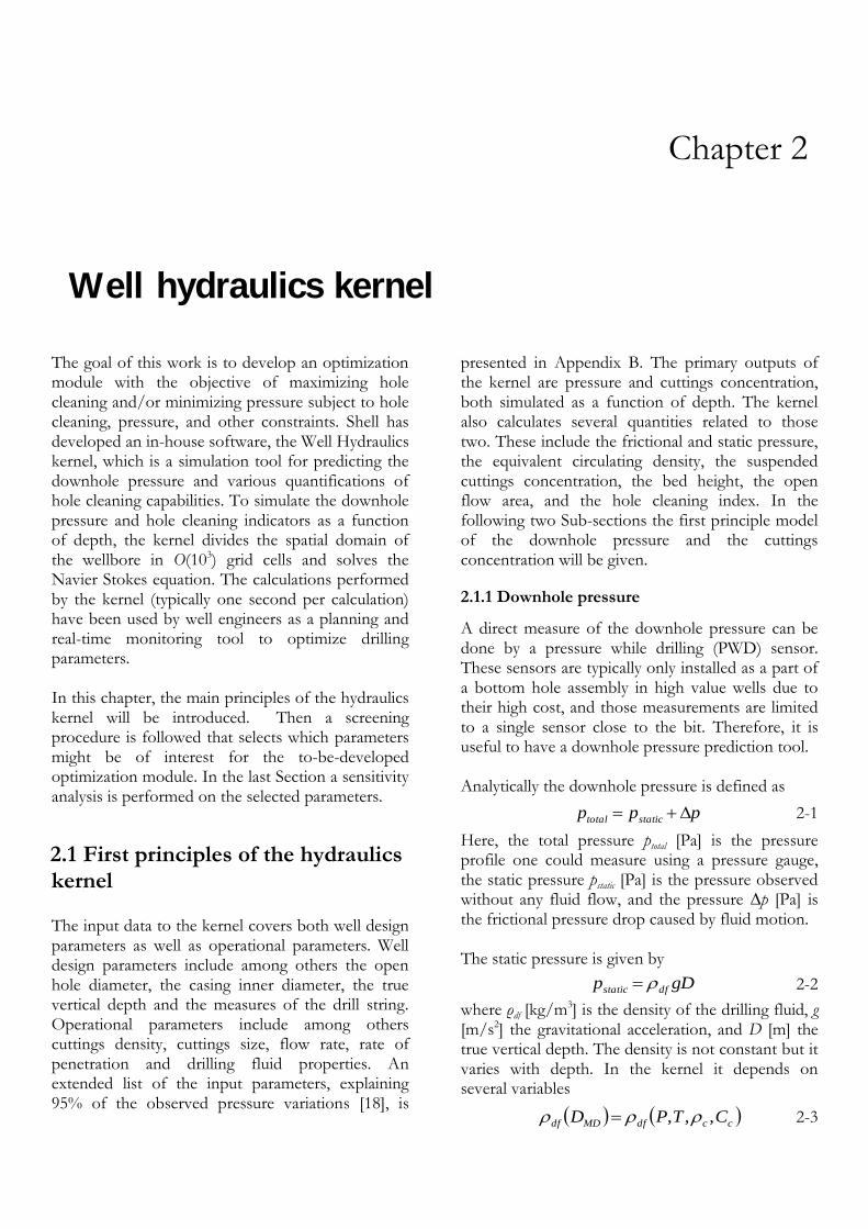
Drill string rotation

Drill string rotation is often required in horizontal wells to achieve proper hole cleaning [22]. As is schematically indicated in Figure 2-2 the cuttings are stirred up by pipe rotation into the high velocity fluid and are subsequently moved up the hole.

Figure 2-2; Cross sectional area of a horizontal well showing the cuttings bed with and without drill string rotation. Areas of low (green) and high (red) velocity do exist [22].

It has been shown that the cuttings concentration depends on multiple factors in a non-linear fashion.

In the kernel other relationships are also included to approximate the cuttings concentration along the entire wellbore as accurately as possible via numerical simulation. Nevertheless, the above description already gives a comprehensive overview of how hole cleaning relates to factors such as cuttings density, rotary speed, flow rate and mud properties.

2.1.3 Output parameters of interest

The to-be-developed optimization module will make use of two outputs of the kernel, i.e., the equivalent circulating density and the hole cleaning index. The equivalent circulating density ρEC [kg/m3] is directly related to the total pressure ptotal and defined as

2-12

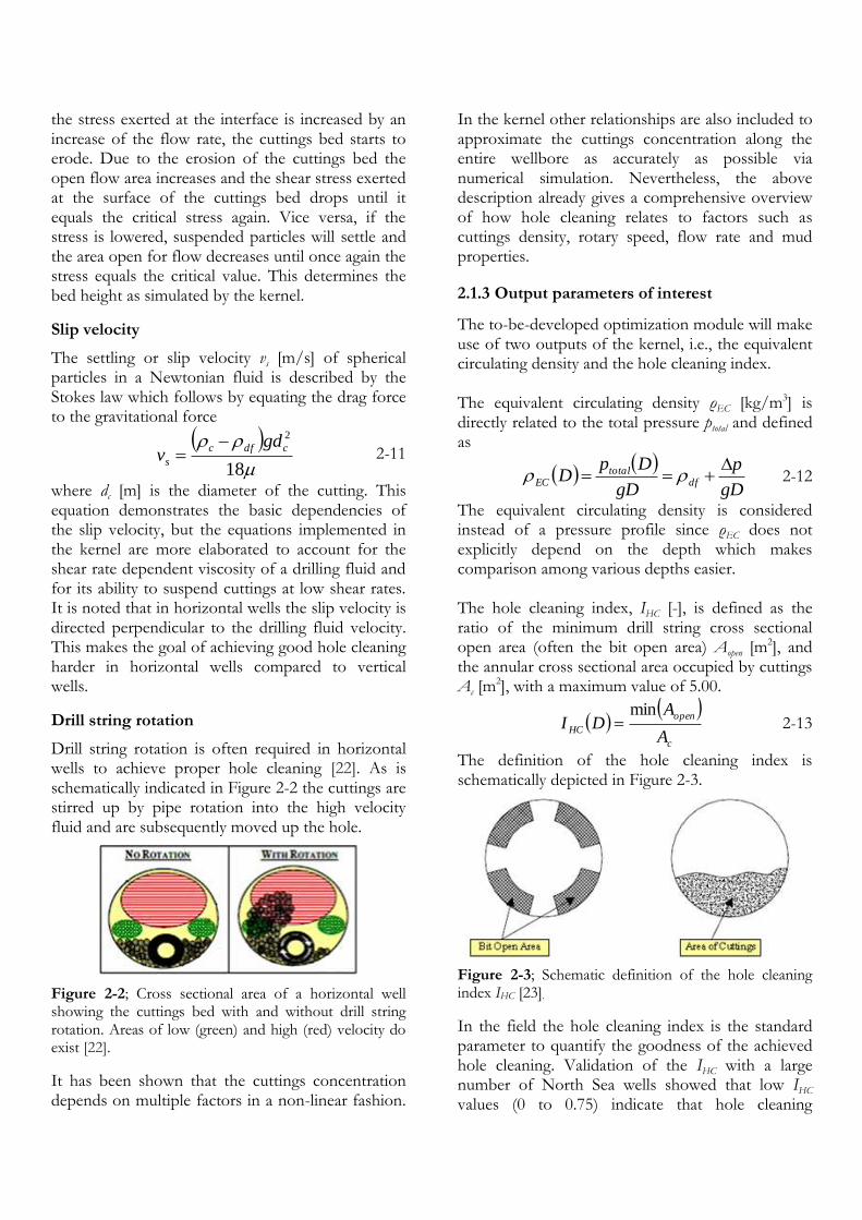
The equivalent circulating density is considered instead of a pressure profile since ρEC does not explicitly depend on the depth which makes comparison among various depths easier. The hole cleaning index, IHC [-], is defined as the ratio of the minimum drill string cross sectional open area (often the bit open area) Aopen [m2], and the annular cross sectional area occupied by cuttings Ac [m

2], with a maximum value of 5.00.

2-13

The definition of the hole cleaning index is schematically depicted in Figure 2-3.

Figure 2-3; Schematic definition of the hole cleaning index IHC [23].

In the field the hole cleaning index is the standard parameter to quantify the goodness of the achieved hole cleaning. Validation of the IHC with a large number of North Sea wells showed that low IHC values (0 to 0.75) indicate that hole cleaning

8

problems are likely and proper hole cleaning procedures should be followed. Intermediate risk exists when the IHC is in the range of 0.75 to 1.25. Larger IHC’s, i.e. IHC > 1.50, correspond to low risk and good hole cleaning [23].

As an example, Figure 2-4 shows a typical equivalent circulating density and hole cleaning index profile for a certain set of input parameters as simulated by the hydraulics kernel.

Figure 2-4; Typical a) equivalent circulation density profile and b) hole cleaning index profile.

2.2 Identification of parameters of interest

The models of the IHC and ρEC as in the hydraulics kernel will later be used in the optimization module. Due to the complexity of these non-linear models resulting in a calculation time of over one second per simulation, proxy models will be created. These proxy models have to capture the input/output

relationships as in the kernel as accurately as possible. To construct meaningful proxy models the inputs significantly contributing to the downhole pressure and hole cleaning have to be identified out of the multi-dimensional input space of the kernel. The mud properties should at least be part of the identified sub-set because the envisioned optimization module calculates the optimal mud properties in the sense that they satisfy the problem statement as given in Chapter 1. Other operational parameters that significantly influence the equivalent circulating density and/or hole cleaning index might also be included in the proxy model and hence later be optimized as well. The drill string dimensions and the borehole geometry are taken as fixed in this study and will not be included in the proxy models. Theis et al [18] performed a statistical analysis on the hydraulics kernel and found that 95% of the variation observed in the pressure profile can be explained by the input parameters presented in Appendix B. Also they found that the following six operational parameters (out of 12 included in Appendix B) have always, so independent of the well design, a significant influence on the pressure profile: the flowrate, the rate of penetration, the cuttings density, the drilling fluid density, and the drilling fluid viscosity parameters k [N/m2.sn] (consistency factor) and n [-] (flow index). A similar study for the hole cleaning index has not yet been performed before. However, based on the physical description given in Section 2.1 it is likely that those six parameters also have a significant influence on hole cleaning, together with the drilling fluid viscosity parameter τ0 [N/m2] (yield stress) and the rotary speed of the drill string vrot [rad/s]. Based on this screening experiment it is decided to develop a code with a functionality to include the aforementioned operational parameters in a proxy model, except the cuttings density. This parameter is not included since it cannot be controlled and optimized, but is rather a consequence of the encountered geology. In addition the code allows the description of the viscosity profile using the Herschel Bulkley parameters k, n, and τ0 as well as the parameters µpv, µyp, and µr6. Preference is given to the latter set, since those are the parameters used in the field. The complete list of selected parameters

1080 1100 1120 1140 1160 1180

0

1000

2000

3000

4000

5000

6000

Equivalent circulating density EC

[kg/m3]

Mea

sure

d d

epth

DM

D [

m]

An equivalent circulating density profile

a)

0 1 2 3 4 5

0

1000

2000

3000

4000

5000

Hole cleaning index IHC

[-]

Mea

sure

d d

epth

DM

D [

m]

A hole cleaning index profile

b)

which can be included as input variables in the proxy models is as follows:

Flow rate Q [m3/s]

Rate of penetration Rp [m/s]

Rotary speed vrot [rad/s]

Drilling fluid density ρdf [kg/m3]

Drilling fluid viscosity o µpv [deg], µyp [deg] and µr6 [deg] or o k [N/m2.sn], n [-] and τ0 [N/m2].

Hence, the number of parameters included in a proxy model, Npar [-], is at most seven. All input parameters not included in this list are assumed to be constant throughout this study, unless specified otherwise.

2.3 Sensitivity analysis of kernel

The behaviour and sensitivity of the kernel its output on the selected parameters can be visualized by varying them one by one over a certain range. For this purpose, each individual input parameter is varied by ±20% around its nominal value and the simulated equivalent circulating density at the bit and average hole cleaning index as simulated along the borehole are plotted in Figure 2-5.

From this one dimensional sensitivity analysis two important features are observed. As expected based on the screening, all parameters plotted do have a significant influence on the output. Secondly, all responses of the kernel within the chosen parameter ranges are smooth and contain a limited amount of curvature. This latter observation gives a first indication that a relatively simple formulation might be sufficient to accurately describe the hole cleaning index and the equivalent circulating density as functions of all these inputs. However, it should be kept in mind that this one dimensional view on the system provides only limited insight since simultaneous variations of multiple parameters might not simply lead to the linear combination of both individual variations due to possible interactions among the parameters. More complex behaviour might be introduced when multiple parameters are varied simultaneously. It is noted that a ±20% variation of the mud weight is, based on mud reports [24] [25], relatively high and will not frequently be required in the field. On the other hand, the variation in the rotary speed of the drill string can easily reach 20%.

Figure 2-5; Visualization of the behavior and sensitivity of a) the equivalent circulating density at the bit and b) the average hole cleaning index on applying a ±20% variation on one input parameter at a time.

Varying the parameter values over a larger range for example 50% does show less smooth behaviour as is shown in Appendix D. This demonstrates already the non-linear character of the kernel. A more complex proxy model would be required to approximate the kernel its behaviour over more extended ranges.

2.4 Conclusions

In this work the hydraulics kernel is used as the foundation for developing the envisioned automatic optimization module. This module will make use of the simulated pressure profile and cuttings concentration profile via two related quantities, namely the equivalent circulating density and the hole cleaning index. The most significant input

80 85 90 95 100 105 110 115 1202.9

2.95

3

3.05

3.1

3.15

3.2

Parameter variation [%]

Aver

age

ho

le c

lean

ing

ind

ex I

HC

,ave

[-]

b)

80 85 90 95 100 105 110 115 1201375

1380

1385

1390

1395

1400

1405

Parameter variation [%]Equiv

alen

t ci

rcula

tin

g d

ensi

ty a

t b

it

EC

,bit [

kg/

m3]

80 85 90 95 100 105 110 115 120

1100

1200

1300

1400

1500

1600

1700

a)

80 85 90 95 100 105 110 115 1201100

1200

1300

1400

1500

1600

1700


Equiv

ale

nt

circula

ting d

ensity a

t th

e b

it

EC

,bit [

kg/m

3]

Flow rate Q

Rate of penetration Rp

Rotatry speed vrot

Mud weight df (right axis)

Plastic viscosity pv

Yield point yp

Low shear yield point r6

80 85 90 95 100 105 110 115 1201100

1200

1300

1400

1500

1600

1700


Equiv

ale

nt

circula

ting d

ensity a

t th

e b

it

EC

,bit [

kg/m

3]

Flow rate Q


Rotatry speed vrot

Mud weight df (right axis)


Yield point yp


10

variables for these quantities are identified, and a one dimensional sensitivity analysis of them within a restricted range showed smooth relations having limited curvature. This gives a first indication that a

relatively simple formulation might be sufficient to accurately capture the input/output structure of the kernel. Finding this formulation is the topic of Chapter 3.

Chapter 3

3Proxy model derivation

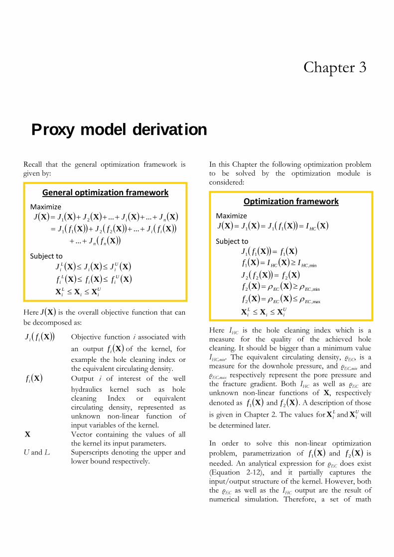
Recall that the general optimization framework is given by:

Here XJ is the overall objective function that can

be decomposed as:

Xii fJ Objective function i associated with

an output Xif of the kernel, for

example the hole cleaning index or the equivalent circulating density.

Xif Output i of interest of the well

hydraulics kernel such as hole cleaning Index or equivalent circulating density, represented as unknown non-linear function of input variables of the kernel.

X Vector containing the values of all the kernel its input parameters.

U and L Superscripts denoting the upper and lower bound respectively.

In this Chapter the following optimization problem to be solved by the optimization module is considered:

Here IHC is the hole cleaning index which is a measure for the quality of the achieved hole cleaning. It should be bigger than a minimum value IHC,min. The equivalent circulating density, ρEC, is a measure for the downhole pressure, and ρEC,min and ρEC,max respectively represent the pore pressure and the fracture gradient. Both IHC as well as ρEC are unknown non-linear functions of X, respectively

denoted as X1f and X2f . A description of those

is given in Chapter 2. The values for L

iX and U

iX will

be determined later. In order to solve this non-linear optimization

problem, parametrization of X1f and X2f is

needed. An analytical expression for ρEC does exist (Equation 2-12), and it partially captures the input/output structure of the kernel. However, both the ρEC as well as the IHC output are the result of numerical simulation. Therefore, a set of math

General optimization framework

Maximize

XXXXX ni JJJJJ ......21

X

XXX

nn

ii

fJ

fJfJfJ

...

...2211

Subject to

XXXU

ii

L

i JJJ

XXXU

ii

L

i fff U

ii

L

i XXX

Optimization framework

Maximize

XXXX HCIfJJJ 111

Subject to

XX 111 ffJ

min,1 HCHC IIf XX

XX 222 ffJ

min,2 ECECf XX

max,2 ECECf XX

U

ii

L

i XXX

12

parLHD NN 20

parNHCHC xxxffII ,...,ˆˆˆ

2111 x

parNECEC xxxff ,...,ˆˆˆ

2122 x

LHD

parparparpar

LHD

LHD

LHD

N

N

i

NNN

N

j

i

jj

N

Ni

xxxx

xxx

xx

xxxx

21

1

2

1

2

11

2

1

1

1

xM

functions is needed that accurately approximates 1f

and 2f , denoted as 1f and 2f . These functions will

be called proxy models and will later serve as objective functions and/or constraints in the optimization module.

3.1 Observed data

The proxy models

3-1

3-2

are built based on (Xi, ρEC,i) and (Xi, IHC,i) data points simulated by the hydraulics kernel by running it NLHD times. These two acquired data sets are called the observed data. The vector x = (x1, x2,… xNpar) is (a subset of) the selected parameter set as derived in Section 2.2, and ρEC,i and IHC,i are scalar values calculated from the ρEC,i vectors and IHC,i vectors, which is primary output of the kernel. For every run, different values of (x1, x2,… xNpar) will be used, while the remaining input parameters will be kept constant. The scenarios to be run are represented by the matrix Mx as:

3-3

Each parameter range xj covers a set of real values between a predefined minimum and maximum. We use latin hypercube design as a method to sample a multi-dimensional space of interest within certain ranges [26]. Latin hypercube design is an experimental design technique that increases the amount of information contained per sample by maximizing the minimum distance among all samples included. This limits the amount of samples needed to get a description accurate enough to use as a base for a proxy model. More details on the latin hypercube design technique can be found in Appendix E. It is noted that an infinite amount of latin hypercube designs exist to sample a given

space. Therefore, every time a design is made, it will be different and result in a unique set of xi vectors. The number of simulation runs needs to be high enough to be able to approximate the original

functions x1f and x2f adequately. For a latin

hypercube design the size of the observed data set, NLHD, has to be at least 20 times the number parameters Npar included in the proxy model, that is:

3-4

The validity of this statement is given in Sub-section 3.5.2. Based on the two acquired data sets, a variety of proxy models can be built. The models considered in this study are

The equivalent circulating density at the bit

The hole cleaning index at the most critical point along the well bore, that is, the worst hole cleaning index encountered

The total hole cleaning index The justification of using these proxy models will be given in the following three Sub-sections. The algorithm to actually calculate the observed data as required to build these proxy models is given in Sub-section 3.1.4.

3.1.1 Equivalent circulating density at the bit

It is sufficient to only build a proxy for the equivalent circulating density at the bit, ρEC,bit = ρEC(D = Dbit) because the cased sections of a well are less vulnerable to too low or too high pressures compared to the open hole section. In addition, ρEC varies relatively slowly with depth (Equation 2-12).

3.1.2 Worst hole cleaning index

Hole cleaning index values below IHC,min = 1.5 mean that there is increased likelihood of drill pipe sticking problems due to cuttings compaction behind the drill bit when pulling out of hole. Ideally one wants to have IHC > 1.5 along the entire well. Maximizing the hole cleaning index explicitly over the entire length of the well would require the same amount of functions to be simultaneously maximized as there are grid cells in the along hole direction. This is not practical since it would result in an equal amount of objective functions as input for the optimization module.

Ry rβ

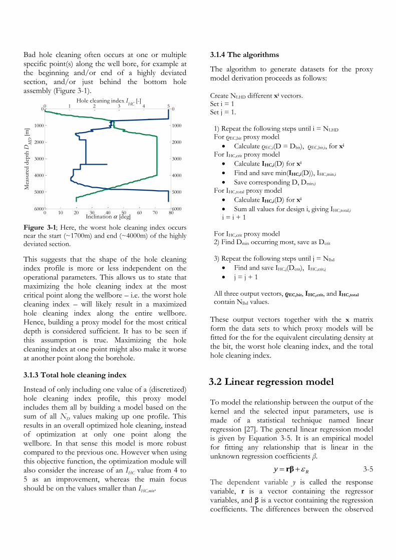
Bad hole cleaning often occurs at one or multiple specific point(s) along the well bore, for example at the beginning and/or end of a highly deviated section, and/or just behind the bottom hole assembly (Figure 3-1).

Figure 3-1; Here, the worst hole cleaning index occurs near the start (~1700m) and end (~4000m) of the highly deviated section.

This suggests that the shape of the hole cleaning index profile is more or less independent on the operational parameters. This allows us to state that maximizing the hole cleaning index at the most critical point along the wellbore – i.e. the worst hole cleaning index – will likely result in a maximized hole cleaning index along the entire wellbore. Hence, building a proxy model for the most critical depth is considered sufficient. It has to be seen if this assumption is true. Maximizing the hole cleaning index at one point might also make it worse at another point along the borehole.

3.1.3 Total hole cleaning index

Instead of only including one value of a (discretized) hole cleaning index profile, this proxy model includes them all by building a model based on the sum of all ND values making up one profile. This results in an overall optimized hole cleaning, instead of optimization at only one point along the wellbore. In that sense this model is more robust compared to the previous one. However when using this objective function, the optimization module will also consider the increase of an IHC value from 4 to 5 as an improvement, whereas the main focus should be on the values smaller than IHC,min.

3.1.4 The algorithms

The algorithm to generate datasets for the proxy model derivation proceeds as follows: Create NLHD different xi vectors. Set i = 1 Set j = 1. 1) Repeat the following steps until i = NLHD For ρEC,bit proxy model

Calculate ρEC,i(D = Dbit), ρEC,bit,i, for xi For IHC,crit proxy model

Calculate IHC,i(D) for xi

Find and save min(IHC,i(D)), IHC,min,i

Save corresponding D, Dmin,i For IHC,total proxy model

Calculate IHC,i(D) for xi

Sum all values for design i, giving IHC,total,i i = i + 1

For IHC,crit proxy model 2) Find Dmin occurring most, save as Dcrit

3) Repeat the following steps until j = Nlhd

Find and save IHC,j(Dcrit), IHC,crit,j

j = j + 1

All three output vectors, ρEC,bit, IHC,crit, and IHC,total contain Nlhd values.

These output vectors together with the x matrix form the data sets to which proxy models will be fitted for the for the equivalent circulating density at the bit, the worst hole cleaning index, and the total hole cleaning index.

3.2 Linear regression model

To model the relationship between the output of the kernel and the selected input parameters, use is made of a statistical technique named linear regression [27]. The general linear regression model is given by Equation 3-5. It is an empirical model for fitting any relationship that is linear in the unknown regression coefficients β.

3-5

The dependent variable y is called the response variable, r is a vector containing the regressor variables, and β is a vector containing the regression coefficients. The differences between the observed

0 10 20 30 40 50 60 70 80

0

1000

2000

3000

4000

5000

6000

Inclination [deg]

Mea

sure

d d

epth

DM

D [

m]

0 1 2 3 4 50

1000

2000

3000

4000

5000

6000


[-]

14

2

1,110ˆ xxy

parpar parpar N

j

jjj

jk

N

j

N

k

kjkj

N

j

jj xxxxy1

2

,

1

1 1

,

1

0ˆ

2

22,2

2

11,1212,122110 xxxxxxy

y-values, yi, and the predicted y-values, ŷi, are the residuals εR. Those are variations in the observed data left unexplained by the linear regression model. This equation includes the important class of polynomial regression models. For example, the second-order polynomial for one parameter, x,

3-6

and the second-order polynomial for two parameters, x1 and x2,

3-7

are linear regression models containing two and five regression variables respectively. The regression variables in the latter equation are two linear, one interaction and two quadratic combinations of the parameters included in the two-dimensional x-vector. All second-order polynomial regression models are covered by

3-8

This equation, or higher order polynomial regression models are widely used in situations where the response is curvilinear, as even complex non-linear relationships can be adequately modeled by polynomials within limited operating ranges. For two or more parameters the regression function is usually called a response surface. They are generally only valid over the range of the parameters contained in the observed data. It is known from the one dimensional sensitivity analysis (Section 2.3) that both the equivalent circulating density as well as the hole cleaning index data show limited curvilinear behavior, which suggests that a second-order polynomial regression model as given by Equation 3-8 may be sufficient to accurately describe them. In Section 3.5 proof will be given why a higher order polynomial regression model is not required. In this study, the response variable ŷ is either ρEC,bit, IHC,crit, or IHC,total, and the x-vector contains Npar of the selected parameter. The values of the regression coefficients β are calculated using stepwise regression.

3.3 Stepwise regression

Fitting a response surface as given by Equation 3-8 can easily lead to over-fitting due to the relatively

large amount of regression coefficients present in the model. In addition, some of the terms included might be insignificant because they show limited or no correlation with the observed data. To prevent the inclusion of unnecessary terms in the proxy model, the stepwise regression algorithm [27] is incorporated in the developed code. This algorithm fits the proxy model to the data by including only a selected subset of the regressor variables, and it proceeds as follows.

1. The algorithm fits an initial proxy model to the observed data using the least squares method. The user can define the regression variables contained in this model. The intercept is always included.

The addition or removal of a subsequent regression variable to or from the proxy model is based on the calculations of p-values (Appendix F). A p-value is scalar value between 0 and 1 quantifying the probability that a regression variable has no correlation with the response variable.

2. Calculate a p-value for all terms not in the current model. If one or multiple terms have a p-value smaller than the pre-set entrance criteria, reject the null hypothesis, add the term with the smallest p-value to the proxy model (this significantly improves the model) and repeat this step. Otherwise, go to step 3.

Rejecting the null hypothesis is like saying that there is a relationship between two phenomena, meaning changes in the regressor variable are related to changes in the response variable. The pre-set entrance criteria is set at 0.05.

3. Calculate a p-value for all terms present in the model. If one or multiple terms have a p-value larger than the pre-set exit criteria, the null hypothesis is accepted, the term with the largest p-value is removed from the proxy model (which does not significantly increase the residual square sum), and go back to step 2. Otherwise, the algorithm stops.

The pre-set exit criteria is set at 0.10. The values of the regression coefficients in the resulting proxy model depend on the model initially fitted to the data. This means that it is not unlikely that a different proxy model will be found when the fitting procedure is repeated on the same data, but now using a different initial model. Both models will be equally accurate in describing their response

variable within the selected subspace. For the sake of consistency, the initial models used in this study will contain all regressor coefficients.

3.4 Summary of proxy model derivation

To build a proxy model, the multi-dimensional parameter space of interest is sampled using a latin hypercube design. Sampling is performed by running simulations resulting in a series of input/output data for the equivalent circulating density and the hole cleaning index. The developed regression models are subsequently fitted to the observed data using stepwise regression. This approach allows for

parametrization of the functions X1f and X2f

over a certain subspace. It has to be evaluated if this parametrization is sufficiently accurate. Therefor the proxy model has to meet several criteria. Those will be introduced in the next Section based on a case study.

3.5 Accuracy of proxy models

The workflow of the developed Matlab code to check a proxy model for its accuracy is demonstrated based on a test case study using real well data. Proxy models are built for ρEC,bit, IHC,crit, and IHC,total based on 161 samples taken from the subspace of flow rate Q, mud weight ρdf, plastic viscosity µpv, and yield point µyp, varied over a range of ±20% with respect to their nominal values as indicated in Table 3-1.

Table 3-1; The subspace used in this case study spans four dimensions ranging ±20% around the nominal parameter values.

Parameter Minimum

value Nominal

value Maximum

value

Q [lit/min] 760 950 1140

ρdf [kg/m3] 992 1240 1488

µpv [deg] 20 25 30

µyp [deg] 13.6 17 20.4

For each of the 161 samples the kernel simulates an equivalent circulating density profile, ρEC, and a hole cleaning index profile, IHC. Those are respectively presented in Figure 3-2 a and b.

Figure 3-2; Plotted for the 161 samples taken from the kernel are the simulated a) equivalent circulating density profiles and b) hole cleaning index profiles.

Based on Figure 3-2b the IHC,crit proxy model is built for the measured depth of 4303m. Among all profiles the hole cleaning index has its lowest value most frequently at this depth, i.e. 101 times. In the following, the constructed proxy models are presented. Their accuracies will be evaluated by introducing multiple criteria. To check those criteria, the code quantifies how well the proxy model fits the data. Secondly it evaluates the predictive capability of the proxy model within the considered subspace, and thirdly it checks two principle assumptions of regression. The last Sub-section discusses approaches for further improvement.

3.5.1 Criteria for fitting accuracy

According to Equation 3-8 building the proxy models considered in this Chapter requires the determination of 15 regression coefficients. Their

1000 1100 1200 1300 1400 1500 1600 1700

0

1000

2000

3000

4000

5000

6000

Equivalent circulating density EC

[kg/m3]

Mea

sure

d d

epth

DM

D [

m]

EC

profiles for all samples

0 1 2 3 4 5

0

1000

2000

3000

4000

5000


[-]

Mea

sure

d d

epth

DM

D [

m]

IHC

profiles for all samples

16

values are summarized in the Table 3-2. It is noted that these values are not unique. Making a new latin hypercube design of equal size over the same subspace and repeating the fit will result in different values for these regressor coefficients. However, both models are built on data taken from the same subspace, and will describe this subspace with the same accuracy.

Table 3-2; The values of the regression coefficients for the proxy models built over the subspace as indicated in Table 3-1. Between brackets the regression variable belonging to the regression coefficient.

Regression coefficient

ρEC,bit(x) IHC,crit(x) IHC,total(x)

ß0 (intercept) 180.9 6.037 1608

ß1 (Q) -1.555*104 -608.6 -5.539*104

ß2 (ρdf) 0.8862 -5.587*10-3 -0.6785

ß3 (µpv) 3.384 0 -5.567

ß4 (µyp) 3.927 0.2286 13.92

ß12 (Q*ρdf) 7.391 0.3658 36.13

ß13 (Q*µpv) -67.66 -2.360 0

ß14 (Q*µyp) -96.00 -14.84 -1380

ß23 (ρdf*µpv) -7.959*10-4 0 2.410*10-3

ß24 (ρdf*µyp) -1.088*10-3 -1.328*10-4 -1.223*10-2

ß34 (µpv*µyp) 1.899*10-2 0 -9.543*10-2

ß11 (Q*Q) 4.247*105 1.819*104 1.461*106

ß22 (ρdf*ρdf) 2.015*10-5 1.280*10-6 1.751*10-4

ß33 (µpv*µpv) 0 9.493*10-4 0.1180

ß44 (µyp*µyp) 3.346*10-2 4.356*10-3 0.6122

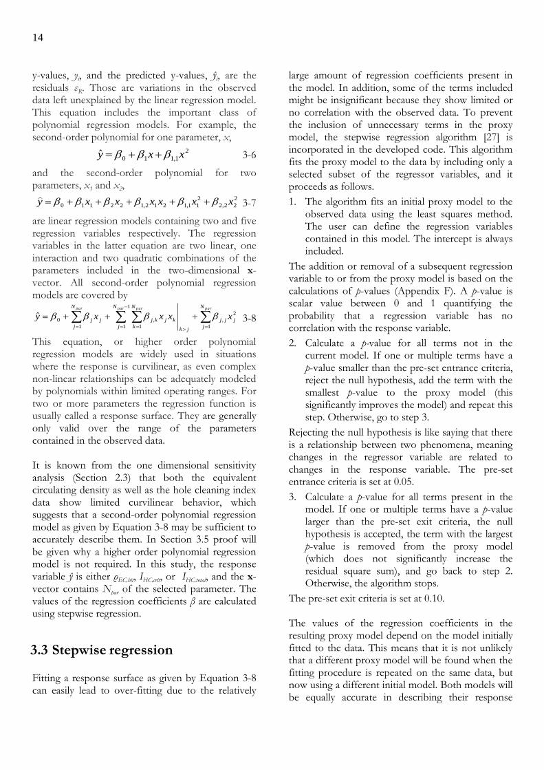
If a regression coefficient equals zero, the stepwise regression algorithm excluded the corresponding regression variable from the proxy model. Just as the values of the regression coefficients, also the regression variables excluded from the proxy model are not identical for every design. For this test case study more regression variables are included in the proxy model than required to fit the observed data set. To keep flexibility for covering a wide range of well configurations with the general formula for a proxy model as given by Equation 3-8, it is decided not to narrow this general form of the proxy model. The multi-dimensional fits made in this study are visualized by plotting the observed responses yi versus the reconstructed responses ŷi. For a perfect model, all points should fall on the line y=x. The plots corresponding to the models presented in Table 3-2 are shown in Figure 3-3.

Figure 3-3; Observed versus reconstructed plots for a) the equivalent circulating density at the bit, b) the worst hole cleaning index, and c) the total hole cleaning index. The red solid line is y=x and serves as a guide to the eye.

By visual inspection of the plots it is observed that a good match is achieved between the observed data as simulated by the kernel, and the reconstructed data as calculated by the proxy model. The fitting

1100 1200 1300 1400 1500 1600 17001100

1200

1300

1400

1500

1600

1700

Observed EC,bit

[kg/m3]

Rec

on

stru

cted

E

C,b

it [

kg/

m3]

Stepwise Regression Model - all

a)

0.8 1 1.2 1.4 1.6 1.8 2 2.2 2.4 2.60.8

1

1.2

1.4

1.6

1.8

2

2.2

2.4

Observed IHC,crit

[-]

Rec

on

stru

cted

IH

C,cri

t [-]


b)

1000 1050 1100 1150 1200 12501000

1050

1100

1150

1200

1250

Observed IHC,total

[-]

Rec

on

stru

cted

IH

C,tot

al [

-]


c)

LHD

LHD

N

i

i

N

i

ii

rec

y

yy

1

1

ˆ

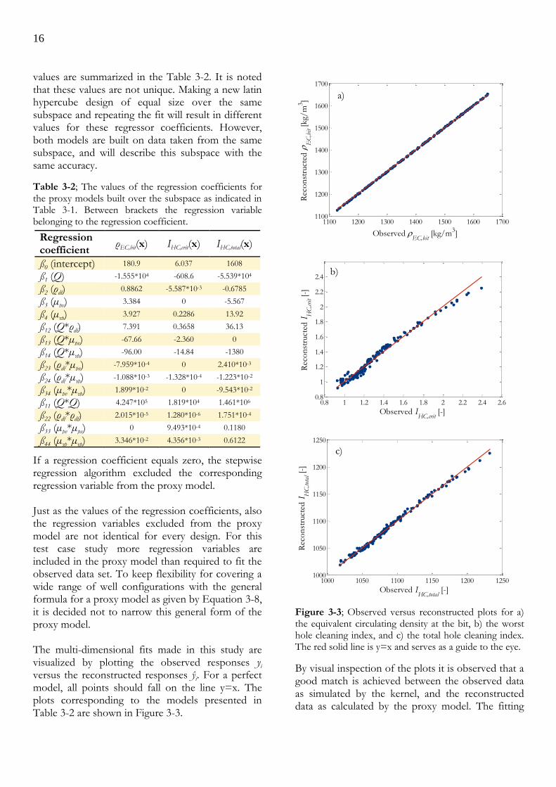
accuracy, δrec, is quantified as the quotient of the absolute residual sum and the observed sum

3-9

For a proxy model to be accepted as fitting the observed data sufficiently accurate, δrec should be smaller than the simulation accuracy of the kernel. Here, the maximum allowed δrec, named δmax, for a proxy model built on (Xi, ρEC,i) and (Xi, IHC,i) data points is set at 1% and 5% respectively. This is to say that it is assumed that the kernel simulates with these accuracies. For the fits presented in Figure 3-3 a, b and c, δrec respectively equals 5.5*10-4, 0.025 and 0.0023. Thus, all three models are accepted based on the criteria for fitting accuracy.

3.5.2 Criteria for predictive capability

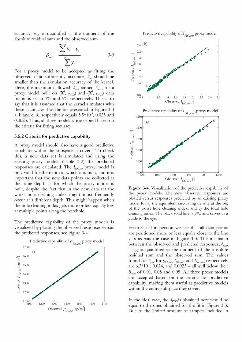
A proxy model should also have a good predictive capability within the subspace it covers. To check this, a new data set is simulated and using the existing proxy models (Table 3-2) the predicted responses are calculated. The IHC,crit proxy model is only valid for the depth at which it is built, and it is important that the new data points are collected at the same depth as for which the proxy model is built, despite the fact that in the new data set the worst hole cleaning index might most frequently occur at a different depth. This might happen when the hole cleaning index gets more or less equally low at multiple points along the borehole. The predictive capability of the proxy models is visualized by plotting the observed responses versus the predicted responses, see Figure 3-4.

Figure 3-4; Visualization of the predictive capability of the proxy models. The new observed responses are plotted versus responses predicted by an existing proxy model for a) the equivalent circulating density at the bit, b) the worst hole cleaning index, and c) the total hole cleaning index. The black solid line is y=x and serves as a guide to the eye.

From visual inspection we see that all data points are positioned more or less equally close to the line y=x as was the case in Figure 3-3. The mismatch between the observed and predicted responses, δpred, is again quantified as the quotient of the absolute residual sum and the observed sum. The values found for δpred for ρEC,bit, IHC,crit, and IHC,total respectively are 6.3*10-4, 0.024, and 0.0023 – all well below their

𝛿max of 0.01, 0.05 and 0.05. All three proxy models are accepted based on the criteria for predictive capability, making them useful as predictive models within the entire subspace they cover.

In the ideal case, the δpred’s obtained here would be equal to the ones obtained for the fit in Figure 3-3. Due to the limited amount of samples included in

1100 1200 1300 1400 1500 1600 17001100

1200

1300

1400

1500

1600

1700

Observed EC,bit

[kg/m3]

Pre

dic

ted

E

C,b

it [

kg/

m3]

Predictive capability of EC,bit

proxy model


a)

0.8 1 1.2 1.4 1.6 1.8 2 2.2 2.4 2.60.8

1

1.2

1.4

1.6

1.8

2

2.2

2.4

Observed IHC,crit

[-]

Pre

dic

ted

IH

C,cri

t [-]

Predictive capability of IHC,crit

proxy model

b)

1000 1050 1100 1150 1200 12501000

1050

1100

1150

1200

1250

Observed IHC,total

[-]

Pre

dic

ted

IH

C,tot

al [

-]

Predictive capability of IHC,total

proxy model


c)

18

1rec

pred

the design, on average a slight increase of the δpred’s can be expected. Here increases of 14.5%, -3.7%, and 0.9% are found respectively, by using

3-10

Those values disclose information about how well the proxy models capture the input/output relationship as in the kernel, but they do contain a relatively large uncertainty. To quantify it, the process of making a latin hypercube design, fitting the data and checking the predictive capability is repeated 100 times. This gives an improved view on these ∆’s, and hence on the accuracy of the proxy models. The results are presented in Table 3-3. Here

rec , pred , and are the averages of the 100

repetitions and rec , pred , and the

corresponding standard deviations.

Table 3-3; Quantification of the proxy models their predictive capability.

Proxy model rec ± rec pred ± pred ±

ρEC,bit (5.6±0.5)*10-4 (6.3±0.5)*10-4 (13±11)%

IHC,crit (2.5±0.3)*10-2 (2.8±0.3)*10-2 (12±11)%

IHC,total (2.4±0.3)*10-3 (2.7±0.2)*10-3 (12±10)%

Comparing rec with the corresponding pred shows

indeed three times an increase, quantified by . The amount of pairs of data included in the

experimental design has a large effect on . In

Appendix G, is plotted as a function of NLHD for

all three proxy models. First a sharp drop of is

observed, and for NLHD < 20Npar is in the order of tens of percentages. For NLHD > 20Npar the drop

is much less sharp and is in the order of percentages. Therefore NLHD should at least be 20 times the amount of parameters included in the proxy model. It is noted that improvements on the proxy model are obtained when increasing NLHD above 20Npar, however they are relatively small. In addition, they come at a cost of a relatively long simulation time, but might still be valuable.

3.5.3 Statistical criteria

Two principle assumptions of linear regression are [27]:

The residuals of the fit are normally distributed.

The variance in the response variable is constant.

If any of those two criteria is violated, the proxy model obtained might not be as representative as required. Hence before accepting a proxy model as sufficiently accurate, the model should as well be checked against those criteria. The distribution of the residuals is visualized by sorting them in bins, and by fitting a normal distribution to the resulting histogram (Figure 3-5).

-4 -3 -2 -1 0 1 2 3 40

5

10

15

20

Sorted EC,bit

residuals [kg/m3]

Fre

quen

cy [

-]a)

-0.1 -0.05 0 0.05 0.1 0.150

2

4

6

8

10

12

14

16

Sorted IHC,crit

residuals [-]

Fre

quen

cy [

-]

b)

Figure 3-5; Histograms of sorted residuals for a) the equivalent circulating density at the bit, b) the worst hole cleaning index, and c) the total hole cleaning index. The red line is a normal distribution fitted to the histogram using the least square method.

Based on those histograms one would not expect inaccurate proxy models, since all histograms can be reasonably described with a normal distribution. This confirms that the code building the proxy model suffices the principle assumption of linear regression that the residuals are normally distributed.

To check the variance in the response variable, the reconstructed responses are plotted versus the residuals (Figure 3-6). In case of constant variance, no structure should be visible in the scatter plot.

Figure 3-6; Scatter plots of reconstructed responses versus the residuals for a) the equivalent circulating density at the bit, b) the worst hole cleaning index, and c) the total hole cleaning index.

The residual plot for ρEC,bit does not show any structure, meaning the variance is constant. This confirms the accuracy of this proxy model. The residual plots for IHC,crit and IHC,total do show structure, meaning not all behaviour present in the observed data is covered by the corresponding proxy model. Despite this structure, the corresponding ∆’s are still well below ∆max as demonstrated in Sub-section 3.5.2. In the next Section two approaches will be discussed to further improve both proxy models.

3.6 Methods to improve proxy model quality

To further improve the proxy models for the hole cleaning index, two measures might be taken:

-8 -6 -4 -2 0 2 4 6 80

2

4

6

8

10

12

14

Sorted IHC,total

residuals [-]

Fre

quen

cy [

-]

c)

1100 1200 1300 1400 1500 1600 1700-8

-6

-4

-2

0

2

4

Reconstructed EC,bit

[kg/m3]

Residual plot for EC,bit

Res

idual

R [

-]

a)

0.8 1 1.2 1.4 1.6 1.8 2 2.2 2.4

-0.2

-0.1

0

0.1

0.2

0.3

Reconstructed IHC,crit

[-]

Residual plot for IHC,crit

Res

idual

R [

-]

b)

1000 1050 1100 1150 1200 1250-20

-15

-10

-5

0

5

10

15

20

Reconstructed IHC,total

[-]

Residual plot for IHC,total

Res

idual

R [

-]

c)

20

Mitigate the strongly skewed distribution of hole cleaning index values.

Increase the size of the design.

The advantages of both approaches are discussed in the following two Sub-sections.

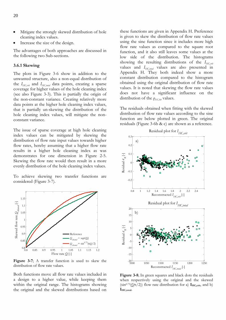
3.6.1 Skewing

The plots in Figure 3-6 show in addition to the unwanted structure, also a non-equal distribution of the IHC,crit and IHC,total data points, creating a sparse coverage for higher values of the hole cleaning index (see also Figure 3-3). This is partially the origin of the non-constant variance. Creating relatively more data points at the higher hole cleaning index values, that is partially un-skewing the distribution of the hole cleaning index values, will mitigate the non-constant variance. The issue of sparse coverage at high hole cleaning index values can be mitigated by skewing the distribution of flow rate input values towards higher flow rates, hereby assuming that a higher flow rate results in a higher hole cleaning index as was demonstrates for one dimension in Figure 2-5. Skewing the flow rate would then result in a more evenly distribution of the hole cleaning index values. To achieve skewing two transfer functions are considered (Figure 3-7).

Figure 3-7; A transfer function is used to skew the distribution of flow rate values.

Both functions move all flow rate values included in a design to a higher value, while keeping them within the original range. The histograms showing the original and the skewed distributions based on

these functions are given in Appendix H. Preference is given to skew the distribution of flow rate values using the sine function since it includes more high flow rate values as compared to the square root function, and it also still leaves some values at the low side of the distribution. The histograms showing the resulting distributions of the IHC,crit values and IHC,total values are also presented in Appendix H. They both indeed show a more constant distribution compared to the histogram obtained using the original distribution of flow rate values. It is noted that skewing the flow rate values does not have a significant influence on the distribution of the ρEC,bit values. The residuals obtained when fitting with the skewed distribution of flow rate values according to the sine function are below plotted in green. The original residuals (Figure 3-6b & c) are shown as a reference.

Figure 3-8; In green squares and black dots the residuals when respectively using the original and the skewed (sin0.75(Qπ/2)) flow rate distribution for a) IHC,crit, and b) IHC,total.

0.8 0.85 0.9 0.95 1 1.05 1.1 1.15 1.20.8

0.85

0.9

0.95

1

1.05

1.1

1.15

Flow rate Q [-]

Skew

ed f

low

rat

e Q

skew

ed [

-]

Reference

Qskewed

= sqrt(Q)

Qskewed

= sin0.75(Q/2)

0.8 1 1.2 1.4 1.6 1.8 2 2.2 2.4

-0.2

-0.1

0

0.1

0.2

0.3


[-]


Res

idual

R [

-]

1000 1050 1100 1150 1200 1250-20

-15

-10

-5

0

5

10

15

20


[-]


Res

idual

R [

-]

1,

skewpred

pred

skew

The plots proof that a more evenly distribution of hole cleaning index values does indeed mitigate non-constant variance among the residuals. Hence, skewing the distribution of flow rate values is a way to improve the proxy model, assuming it contains the flow rate as one of its parameters. Especially for the higher values of IHC,crit and IHC,total the variance becomes more constant. To quantify the improvement made in both models, the process of making a latin hypercube design, skewing the distribution of flow rate values, fitting the data, and checking the predictive capability is repeated 100 times. The values found here for δpred, will be called δpred,skew. Those are compared to the values found for δpred, when using the original flow rate distribution (Table 3-3), via

3-11

The results are presented in Table 3-4. Here pred ,

skewpred, , skew are the averages of the 100

repetitions and pred , skewpred, , and skew , the

corresponding standard deviations.

Table 3-4; Quantifying the effect of skewing the distribution of flow rate values. The values in the second column are taken from Table 3-3.

Proxy model

pred ±

pred

skewpred, ±

skewpred,

skew ±

skew

IHC,crit (2.8±0.3)*10-2 (2.4±0.3)*10-2 (19±16)%

IHC,total (2.7±0.2)*10-3 (2.4±0.3)*10-3 (12±13)%

Comparing pred with skewpred, shows indeed an

improvement for the IHC,crit and for the IHC,total proxy model. On average an improvement of 19% and 12% is respectively made.

3.6.2 Larger design

A second measure possibly improving the proxy models is the inclusion of more pairs of data in the latin hypercube design as shown in Appendix G. However, when sufficient data is already included in the initial design, including even more data will no longer improve the proxy model. Below the reconstructed versus residuals plots obtained when using a design of NLHD = 200Npar = 800 are presented. As a reference the reconstructed versus

residuals plots of Figure 3-6 are included, where NLHD = 4Npar + 1 = 161.

Figure 3-9; In orange squares and black dots the residuals when respectively using the original (NLHD = 161) and the enlarged (NLHD = 800) design for a) ρEC,bit, b) IHC,crit, and c) IHC,total. No skewing is applied.

1100 1200 1300 1400 1500 1600 1700-8

-6

-4

-2

0

2

4

Reconstructed EC,bit

[kg/m3]

Residual plot for EC,bit

Res

idual

R [

-]

0.8 1 1.2 1.4 1.6 1.8 2 2.2 2.4

-0.2

-0.1

0

0.1

0.2

0.3


[-]


Res

idual

R [

-]

1000 1050 1100 1150 1200 1250-20

-15

-10

-5

0

5

10

15

20


[-]


Res

idual

R [

-]

22

1arg,

arg elpred

pred

el

There is no significant difference observed between the residual plots using NLHD = 161 and NLHD = 800. To quantify the difference in accuracy of both proxy models, the process of making a latin hypercube design with NLHD = 800, fitting the data, and checking the predictive capability is repeated 100 times. The values found here for δpred, will be called δpred,large. Those are compared to the values found for δpred, when using the smaller design (Table 3-3), via

3-12

The results are presented in Table 3-5. Here pred ,

elpred arg, , el arg are the averages of the 100

repetitions and pred , elpred arg, , and el arg ,

the corresponding standard deviations.

Table 3-5; Quantifying the effect of enlarging the design. The values in the second column are taken from Table 3-3.

Proxy model

pred ±

pred

elpred arg, ±

elpred arg,

el arg ±

el arg

ρEC,bit (6.3±0.5)*10-4 (6.0±0.2)*10-4 (5±8)%

IHC,crit (2.8±0.3)*10-2 (2.7±0.1)*10-2 (5±9)%

IHC,total (2.7±0.2)*10-3 (2.55±0.09)*10-3 (5±9)%

Comparing pred with the corresponding elpred arg,

shows indeed in all three cases a slight decrease,

quantified by el arg . This confirms an improvement

of the proxy model - be it a small one - is made by using more samples. Taking into account the additional simulation time required, one might judge this improvement too expensive.

3.6.3 Discussion

Two approaches worth considering improving a proxy model were presented in this Section. The approach of enlarging the design comes at a cost since it requires running more simulations. The improvements which can still be made depend on the amount of data points already included in the initial design. On the other hand, the skewing approach is free and does not require additional simulation time. The introduced skewing procedure takes away a significant amount of the non-constant

variance observed in the residual plots for IHC,crit and IHC,total proxy model, thereby increasing the predictive capability. In Chapter 4 and Chapter 5, all proxy models will be built using a sufficient amount of data points and a skewed distribution of the flow rate values. Skewing will be done according to the sine function as introduced in Figure 3-7.

3.7 Conclusions and recommendations

A workflow to obtain expressions for the proxy

models x1f and x2f has been identified. Using

this workflow the input/output structure of the hydraulics kernel can accurately be captured within a given subspace. Second-order polynomial regression models proved to be adequate for this purpose, meaning higher order regressor variables were not required. To achieve sufficient accuracy a minimum number of samples should be taken from the kernel, at least twenty times the number of parameters included in the proxy model. When the flow rate is included as one of the parameters in a proxy model for the hole cleaning index, it is advised to skew the distribution of the flow rate values, since this significantly improves the proxy model. One of the limitations of the proxy models is that they cannot be accurately built over large ranges and simultaneously include a large amount of parameters. After constructing a proxy model one should always check its predictive capability and the variance in the residuals before accepting the model as an accurate representation of a subspace of the kernel. Being able to build an accurate proxy model now opens the opportunity to predict optimal mud properties and other operational parameters included in the models, by using the developed proxy models as objective functions and/or constraints in the optimization module. This will be the topic of Chapter 4.

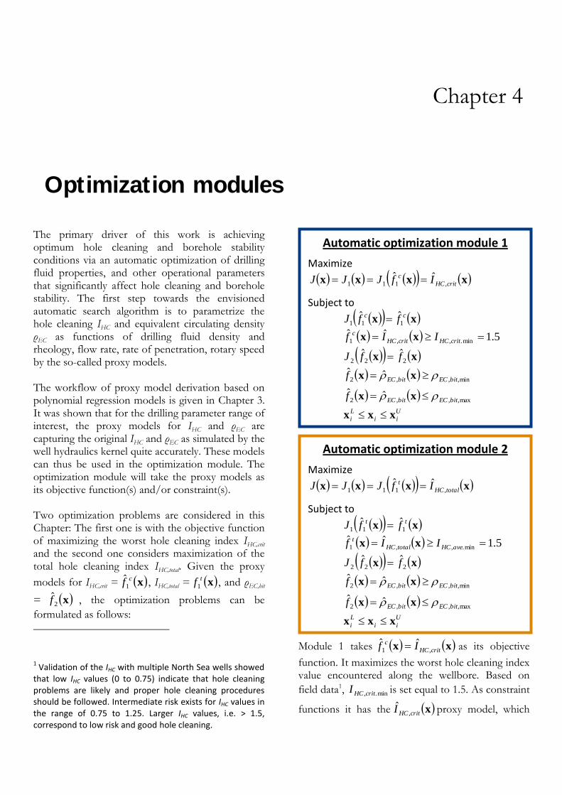
Chapter 4

4Optimization modules

The primary driver of this work is achieving optimum hole cleaning and borehole stability conditions via an automatic optimization of drilling fluid properties, and other operational parameters that significantly affect hole cleaning and borehole stability. The first step towards the envisioned automatic search algorithm is to parametrize the hole cleaning IHC and equivalent circulating density ρEC as functions of drilling fluid density and rheology, flow rate, rate of penetration, rotary speed by the so-called proxy models. The workflow of proxy model derivation based on polynomial regression models is given in Chapter 3. It was shown that for the drilling parameter range of interest, the proxy models for IHC and ρEC are capturing the original IHC and ρEC as simulated by the well hydraulics kernel quite accurately. These models can thus be used in the optimization module. The optimization module will take the proxy models as its objective function(s) and/or constraint(s). Two optimization problems are considered in this Chapter: The first one is with the objective function of maximizing the worst hole cleaning index IHC,crit and the second one considers maximization of the total hole cleaning index IHC,total. Given the proxy

models for IHC,crit = xcf1ˆ , IHC,total = xtf1 , and ρEC,bit

= x2f , the optimization problems can be

formulated as follows: 1

1 Validation of the IHC with multiple North Sea wells showed

that low IHC values (0 to 0.75) indicate that hole cleaning problems are likely and proper hole cleaning procedures should be followed. Intermediate risk exists for IHC values in the range of 0.75 to 1.25. Larger IHC values, i.e. > 1.5, correspond to low risk and good hole cleaning.

Module 1 takes xx critHC

c If ,1ˆˆ as its objective

function. It maximizes the worst hole cleaning index value encountered along the wellbore. Based on

field data1, min.,critHCI is set equal to 1.5. As constraint

functions it has the xcritHCI ,ˆ proxy model, which

Automatic optimization module 1

Maximize

xxxx critHC

c IfJJJ ,111ˆˆ

Subject to

xx cc ffJ 111ˆˆ

5.1ˆˆmin.,,1 critHCcritHC

c IIf xx

xx 222ˆˆ ffJ

min,,,2ˆˆ

bitECbitECf xx

max,,,2ˆˆ

bitECbitECf xx

U

ii

L

i xxx


Maximize

xxxx totalHC

t IfJJJ ,111ˆˆ

Subject to

xxtt ffJ 111ˆˆ

5.1ˆˆmin.,,1 aveHCtotalHC

t IIf xx

xx 222ˆˆ ffJ

min,,,2ˆˆ

bitECbitECf xx

max,,,2ˆˆ

bitECbitECf xx

U

ii

L

i xxx

24

12 parNN

0x

D

totalHC

aveHCN

II

,

,

should be bigger than min.,critHCI , and the xbitEC ,

proxy model which should be bigger than the pore pressure and smaller than the fracture gradient

respectively represented by min,,bitEC and max,,bitEC .

Module 2 takes xx totalHC

t If ,1ˆˆ as its objective

function. It maximizes the sum of all ND hole cleaning index values, with ND the number of grid cells in which the spatial domain of the wellbore is subdivided. As constraint functions it has the

xbitEC , proxy model, which should again fall

within min,,bitEC and max,,bitEC , and the xtotalHCI ,ˆ

proxy model, which should be larger than min.,aveHCI .

The average hole cleaning index aveHCI , is defined as

4-1

Ideally one wants to obtain a hole cleaning index profile bigger than 1.5 for all depth points ND. This optimization module is solving the whole profile instead of every depth point, so a constraint is set on the average hole cleaning index as 1.5. The solution to an optimization problem is the critical point of the so-called Lagrangian function L(x,λ) [28]. This critical point is calculated by equating the gradient of the Lagrangian function to zero. For details about this analytical formulation of the optimization problem see Appendix I. Due to the non-linear constraints both optimization problems cannot be solved analytically. Hence both optimization problems will be solved numerically.

4.1 Inputs for numerical optimization

The optimization problems given in the introduction of this Chapter are non-linear, constrained optimization problems. To solve them, the Matlab optimization function fmincon will be used with the sequential quadratic programming algorithm. This steepest descent method is one of the most effective algorithms to solve non-linear constrained optimization problems [29]. The method can only minimize an objective function. A maximization problem is dealt with by multiplying the objective function by -1. The inputs to the

function fmincon, used by the sequential quadratic programming algorithm, are:

An objective function describing a dependent parameter ŷ as a function of independent vector x.

A lower bound xL and an upper bound xU so that the solution xopt is found in the range xL ≤ xopt ≤ xU.

The non-linear constraints it has to adhere to.

An initial point x0 in the range xL ≤ x0 ≤ xU from where the algorithm starts its search.

It is shown in Chapter 3 that the proxy models form a precise description of the kernel within the entire space they cover. There is no reason to limit our search for xopt to a subspace of the space covered by the proxy model. Neither it is justifiable to expand our search for xopt over a space bigger than the space covered by the proxy model, since it is only valid within the space it is build. Hence, the lower bound xL and the upper bound xU will in both optimization modules be set equal to the ones used to build the proxy models. The algorithm finds its way to xopt by moving in the way of the steepest descent. If the initial point x0 is not chosen close enough to xopt, the optimization algorithm might end up in a local minimum, instead of the global minimum. To prevent this, multiple initial points should be given to the algorithm and at the end the best solution should be selected. In this study, the nominal x vector is taken as an initial points, just as all vectors x that can be made by combining values from the xL and xU vector, for example, [QU ρdf,U µpv,L µyp,L µr6,U]. The number of initial points is given by

4-2

After also having defined suitable values for IHC,min, ρEC,bit,min, and ρEC,bit,max, the function fmincon is set to solve the optimization problem. In case it cannot find a solution satisfying all three constraints, it repeats the optimization process without the constraint on the hole cleaning index. Due to the efficiency of the sequential quadratic programming algorithm, the optimization modules constructed are fast. The calculation time to arrive at the solution xopt is in the order of seconds.

4.2 Analysis of objective function

The objective functions themselves contain only one extreme point due to their quadratic nature. This can easily be shown by equating all partial derivatives of Equation 3-8 to zero. The resulting system of equations has one solution. Next to a minimum, the extreme point xE of the objective function can also be a maximum or, most probably, a saddle point. It can also be located outside the considered space, that is xE < xL or xE > xU. Hence the optimization algorithm will most likely not end up in the extreme point of the objective function. Multiple local extreme points are added to the optimization problem by the imposed constraints in the form of xL, xU, and the three constraint functions. It is more likely that the optimization algorithm ends up in one of these points. As an illustration of where extreme points are located, consider the objective function IHC,crit(Q,µpv) = ß0 + ß1Q + ß2µpv + ß12Qρdf + ß11Q

2 + ß22µpv2, which

is a two-dimensional form of Equation 3-8, with regression coefficients ß0 = 6.99*10-1, ß1 = -1.55*102 s/m3, ß2 = 7.71*10-2 deg-1, ß12 = -4.23 s/m3.deg-1, ß11 = 1.05*104 s2/m6, and ß22 = 0deg-2. The function has a saddle point and is plotted in Figure 4-1. The red box indicates the domain where data is taken from the kernel and hence the domain where the proxy model is valid.

Figure 4-1; As an example, the objective function IHC,crit(Q,µpv) with its extreme point located at (Q ; µpv) = (1.83*10-2 ; 5.41*101). The red square indicates the range of interest.

The vector xopt can only be found within or on the edge the domain enclosed by the red line. The

amount of points where the optimization algorithm might end up is further limited because the objective function itself is smooth and does not contain any maxima within the domain of interest. This domain might be further restricted by the constraints imposed on the equivalent circulating density. The ρEC,bit objective function corresponding to the IHC,crit objective function as presented in Figure 4-1 is shown in Figure 4-2. The function is only plotted over the domain that is enclosed by the red box. The four curves superimposed on the plotted surface represent various fracking gradients. The red, yellow, green, and blue curve respectively corresponds to a value for ρEC,bit,max of 1270, 1280, 1290, and 1300kg/m3.

Figure 4-2; Depending on the constraint value for ρEC,bit,max, xopt can be found within a certain domain.

The solution xopt has to be found in the parameter space resulting in ρEC,bit ≤ ρEC,bit,max. The higher the value for ρEC,bit,max, the larger the corresponding domain. For values a bit lower than 1270kg/m3 a solution to the optimization problem can no longer be found. For values slightly higher than 1300kg/m3 the solution can be found within the entire domain. In Figure 4-3 the same objective function is shown as in Figure 4-1, but only the part enclosed by the red box. The constraint as might be set by ρEC,bit,max is also included.

0.01 0.015 0.02 0.02510

15

20

25

30

35

40

45

Flow rate Q [m3/s]

Objective function IHC,crit

Pla

stic

vis

cosi

ty

pv [

deg

]

1

1.5

2

2.5

3

3.5

4

0.014

0.016

0.018

20

25

30

1260

1280

1300

1320


[deg]

Objective function EC,bit

Flow rate Q [m3/s]

1270

1275

1280

1285

1290

1295

1300

26

Figure 4-3; The solution xopt can only be found below the ρEC,bit,max constraint.

Looking at the shape of this objective function with the imposed constraint directly reveals where the optimization module will end up given a pore pressure and a fracture gradient. Assuming that the pore pressure gradient is located below the here considered ρEC,bit range, and knowing that this objective function slightly increases for the maximum value of Q, shows that if a solution is found, it will be found for the minimum value of the plastic viscosity. Due to the nature of the hydraulics kernel, and the type of constraints imposed, the optimal solution will often partially be found at the boundary of the domain of interest. The analysis presented in this Section applies as well for optimization problems containing higher dimensional objective functions, but within only two dimensions it can nicely be visualized.

4.3 Test case study

Continuing the test case study of Section 3.5, here the results obtained via both optimization modules are presented.

Module 1 and module 2 take respectively xcf1ˆ =

IHC,crit(x) and xtf1

ˆ = IHC,total(x) as their objective

function, as given in Table 3-2. As mentioned in Chapter 3, these proxy models are not unique in the sense that different values for the regressor coefficients will be found using a new data set. Still, each model describes the same subspace with a high accuracy. For both modules the solution xopt has to

be found within the range xL ≤ xopt ≤ xU, where xL and xU are as given in Table 3-1. The non-linear constraint functions are made up of the three proxy models (see again Table 3-2), and the three scalar values which equal in this test case study:

ρEC,bit,min = 1240kg/m3

ρEC,bit,max = 1380kg/m3

IHC,min = 1.5

According to Equation 3-8, 17 different initial points x0 will be used by both optimization algorithms to reduce the change of ending up in a local minimum. The calculated optimal parameter values, together with their upper and lower bounds as a reference, are presented in Table 4-1.

Table 4-1; Optimized parameter values obtained using optimization module 1 and 2. The lower and upper bounds are shown for reference.

Parameter xopt,1

(module 1)

xopt,2 (module 2)

Lower bound

Upper bound

Q [lit/min] 1140 1140 760 1140

ρdf [kg/m3] 1238 1221 992 1488

µpv [deg] 20 30 20 30

µyp [deg] 13.6 13.6 13.6 20.4

Both optimization modules find the same optimal value for the flow rate Q and the yield point µyp. For the mud weight µdf there is a slight difference. Optimization module 1 and 2 find the optimal value for the plastic viscosity µpv at the very low and very high end of the range covered. In addition, the optimum values for flow rate and yield point are also found at the edge of the covered space. Apparently the subspace in which xopt can be found is not only bounded by the non-linear constraint functions, but also partially by xL and xU, see also Figure 4-1. Having these optimum values for the parameters, it is interesting to see the resulting response variables, the two hole cleaning index profiles, and the two downhole total pressure profiles. In the tables below the responses of the three proxy models are summarized for xopt,1 and xopt,2. The average hole cleaning index IHC,ave is also included. A comparison between the responses of the proxy models and the simulated responses of the kernel is made. To quantify the accuracy of the proxy model in the optimal points, δpred is also included in the tables.

0.014

0.016

0.018

20

25

30

0.5

1

1.5

2


[deg]

Objective function IHC,crit

Flow rate Q [m3/s]

0.9

1

1.1

1.2

1.3

1.4

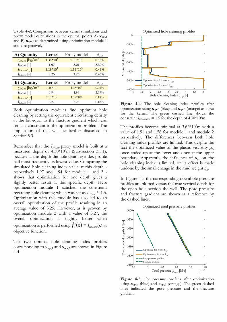
Table 4-2; Comparison between kernel simulations and proxy model calculations in the optimal points A) xopt,1 and B) xopt,2 as determined using optimization module 1 and 2 respectively.

A) Quantity Kernel Proxy model δpred ρEC,bit [kg/m3] 1.38*10

3 1.38*10

3 0.16%

IHC,crit [-] 1.97 2.01 2.30%

IHC,total [-] 1.16*103 1.16*10

3 0.46%

IHC,ave [-] 3.25 3.26 0.46%

B) Quantity Kernel Proxy model δpred ρEC,bit [kg/m3] 1.38*103 1.38*103 0.06%

IHC,crit [-] 1.94 1.99 2.39%

IHC,total [-] 1.17*103 1.17*103 0.18%

IHC,ave [-] 3.27 3.28 0.18%

Both optimization modules find optimum hole cleaning by setting the equivalent circulating density at the bit equal to the fracture gradient which was set as a constraint to the optimization problem. The implication of this will be further discussed in Section 5.3. Remember that the IHC,crit proxy model is built at a measured depth of 4.30*103m (Sub-section 3.5.1), because at this depth the hole cleaning index profile had most frequently its lowest value. Comparing the simulated hole cleaning index value at this depth - respectively 1.97 and 1.94 for module 1 and 2 - shows that optimization for one depth gives a slightly better result at this specific depth. Here optimization module 1 satisfied the constraint regarding hole cleaning which was set as IHCcrit ≥ 1.5. Optimization with this module has also led to an overall optimization of the profile resulting in an average value of 3.25. However, as is proven by optimization module 2 with a value of 3.27, the overall optimization is slightly better when

optimization is performed using xtf1

ˆ = IHC,total(x) as

objective function. The two optimal hole cleaning index profiles corresponding to xopt,1 and xopt,2 are shown in Figure 4-4.

Figure 4-4; The hole cleaning index profiles after optimization using xopt,1 (blue) and xopt,2 (orange) as input for the kernel. The green dashed line shows the constraint IHC,crit,min = 1.5 for the depth of 4.30*103m.

The profiles become minimal at 3.62*103m with a value of 1.51 and 1.58 for module 1 and module 2 respectively. The differences between both hole cleaning index profiles are limited. This despite the fact the optimized value of the plastic viscosity µpv once ended up at the lower and once at the upper boundary. Apparently the influence of µpv on the hole cleaning index is limited, or its effect is made undone by the small change in the mud weight ρdf. In Figure 4-5 the corresponding downhole pressure profiles are plotted versus the true vertical depth for the open hole section the well. The pore pressure and fracture gradient are shown as a reference by the dashed lines.

Figure 4-5; The pressure profiles after optimization using xopt,1 (blue) and xopt,2 (orange). The green dashed lines indicated the pore pressure and the fracture gradient.

1 1.5 2 2.5 3 3.5 4 4.5 5-6000

-5000

-4000

-3000

-2000

-1000

0

Hole Cleaning Index IHC

[-]

Mea

sure

d d

epth

[m

]

Optimized hole cleaning profiles

Optimization for worst IHC

Optimization for total IHC

3.8 4 4.2 4.4 4.6 4.8

x 104

-3450

-3400

-3350

-3300

-3250

-3200

-3150

Total pressure ptotal

[kPa]

Tru

e ver

tica

l d

epth

D [

m]

Optimized total pressure profiles

Optimized for worst IHC

Optimization for total IHC

Pore pressure gradient

Fracture gradient

28

As imposed by two constraints, after optimization the downhole pressure falls between the pore pressure and the fracture gradient. It is located close to the fracture gradient since this leads to the best hole cleaning. In case one prefers keeping a larger safety margin, one can lower the ρEC,bit,max value and repeat the optimization. This is further discussed in Section 5.3. The workflows of the optimization modules have been demonstrated in this Section based on a test case study. The differences between the hole cleaning index profiles as simulated for xopt,1 and xopt,2 turned out to be very limited, despite the different value calculated for the optimum plastic viscosity.

4.4 Optimization check

To check the optimization algorithm, an exhaustive search is performed. It should be ensured that the vector x which is identified by the optimization modules as xopt does indeed contain the optimal parameter values. For each parameter optimized, a vector with the values xL : dx : xU is constructed, with dx the step size. To get a fair check, dx should not be too big, on the other hand, to prevent issues with matrix multiplications in Matlab, it should neither be too small. In the optimization algorithm dx is as in the following table.

Table 4-3; Step sizes used per parameter during exhaustive search.

Parameter xi Unit Step size dx

Flow rate Q lit/min 20

Rate of penetration Rp m/h 1

Rotary speed vrot rpm 2

Mud weight ρdf kg/m3 10

Plastic viscosity µpv deg 1

Yield point µyp deg 1

6 rpm Fann reading µr6 deg 1

For the test case study discussed in the previous Section, this comes down to 6.4*104 possible combinations of parameter values. The developed

proxy models can calculate the corresponding vectors ρEC,bit, IHC,crit and IHC,total via three matrix multiplications within the order of seconds. The non-linear constraints are subsequently imposed on the resulting data set by removing the ρEC,bit, IHC,crit and IHC,total values from the vectors when the corresponding parameter combination results either in ρEC,bit > ρEC,bit,max or in ρEC,bit < ρEC,bit,min. Subsequently for module 1 and module 2 the optimal parameters xopt,exh are found by respectively selecting the highest IHC,crit or IHC,total value from the remaining values. In case that xopt,exh differs less than dx from the vector found by the optimization module xopt is accepted. If the difference is higher than dx it is likely that not sufficient points have been included in the latin hypercube design. Increasing the observed data set often results in the elimination of this issue.


The workflow for building accurate proxy models together with the optimization procedure described in this Chapter creates the envisioned automatic set point search algorithm. Two optimization modules with different objective functions are introduced in this Chapter. Based on the test study case, both optimization modules give more or less equally good hole cleaning, and satisfy the three non-linear constraints. The solution found by numerical optimization is crosschecked with an exhaustive search to confirm that the function fmincon has indeed found the optimal solution. This algorithm can be used as a standardized way and systematic planning tool prior to drilling a well to efficiently find optimum values subjected to multiple constraints, which is difficult to do by hand. Also when real-time data leads to an update of the pore pressure and/or the fracture gradient, the algorithm allows for a quick recalculation of the optimum values.

xx 111ˆˆ ffJ

xx 222ˆˆ ffJ

Chapter 5

5Case studies & Cost functions

The main driver of this work is optimizing hole cleaning and borehole stability. For this purpose two automatic setpoint search algorithms have been developed. The improvements that could have been made by using one of these algorithms are quantified by evaluating two case studies based on real field data. The first case study will be coupled to a borehole stability analysis. Firstly the hole cleaning index and equivalent circulating density profile will be simulated using the parameter values as used in the field. Secondly the developed search algorithm will find the optimal values given among others the parameter ranges as in the drilling fluid program as constraints. In the following it is assumed that all parameter values within these ranges are equally expensive. However, in the field one will probably face higher costs when for example increasing the flow rate by 100 litres per minute. In this case the pumps would wear faster and consume more energy. This would make it worth considering if an improvement of the hole cleaning by increasing the flow rate is indeed worth the investment one has to make regarding the additional pump costs. The topic of valuating certain settings for the operational parameters is beyond the scope of this thesis. Section 5.3 will reconsider the optimization modules as introduced in Chapter 4, leading to

5-1

5-2

As stated previously, the downhole pressure should fall between the pore pressure and the fracture gradient. However, preferably the downhole pressure is located in the middle, and shifted more towards the pore pressure gradient. This makes that

setting the downhole pressure equal to the pore pressure or fracture gradient with the intention to increase hole cleaning comes at a cost. An improvement of the hole cleaning should therefore be related to how much further the downhole pressure approaches one of the gradients. All proxy models used in this Chapter to calculate the optimal drilling fluid properties are checked against and accepted based on the criteria introduced in Section 3.5.

5.1 Case study I

Recall that prior to running the optimization module constraints have to be set for the equivalent circulating density in terms of the minimum required and maximum allowed equivalent circulating density. The maximum allowable equivalent circulating density equals the fracture gradient and is predicted based on leak of tests, and on knowledge gained from offset wells. The minimum downhole pressure is reached in the static period, and is determined by the density of the drilling fluid. Borehole stability (BHS) software is used to predict the minimum mud weight required to drill a well (section) to ensure borehole stability and prevent inflow of formation fluids at all times – also in static periods when the downhole pressure is considerably lower compared to when flowing. The envisioned workflow for the developed optimization module in combination with this BHS software is further elaborated on in this Section based on a first case study.

30

Workflow of borehole stability software

The workflow for borehole stability analysis using the BHS software is first to build a BHS model based on input data known from measurements and/or estimates. This data comprises formation strength and stresses, in-situ pressures, and well bore geometry. Then the BHS model is calibrated with offset well observations. Once properly calibrated, it is used to predict the minimal mud weight requirement. Potential in real-time acquired data might later lead to an update of the model. In some cases, there would be sufficient information from the offset wells (e.g. comparable inclination/azimuth, etc.) to deduce the minimum mud weight required for the planned well. This would be deemed sufficient and BHS modelling may not be needed. In cases where the planned well would have a different inclination than any of the offset wells - or in the absence of relevant offset wells - it is needed to run BHS calculations to check for the minimum mud weight requirement.

Well description

The well considered here – Well I – is an S type production well in the North Sea targeting the Rotliegend sandstone formation at a true vertical depth of 3985m. The Ieper clay is located at a depth D of 1000m to 1515m, and is drilled with a 12¼’’ bit [25]. The targeted mud properties as stated in the drilling fluid program are presented in Table 5-1.

Table 5-1; Targeted drilling fluid properties as taken from the drilling fluid program [25].

Parameter Lower bound

Upper bound

Mud weight ρdf [sg] 1.35 1.42

Plastic viscosity µpv [deg] As low as possible

Yield point µyp [deg] 23.4 32.8

6 rpm Fann reading µr6 [deg] 9.4 14

For the parameters which can be included in the proxy model, the input parameter values of the field are summarized in Table 5-2. For the remaining values, including the well trajectory, see Appendix C.

Table 5-2; Average field values of the mud properties and of the other operational parameters which can be included in the proxy models.

Parameter Field value

Mud weight ρdf [sg] 1.42

Plastic viscosity µpv [deg] 24

Yield point µyp [deg] 33

6 rpm Fann reading µr6 [deg] 10

Flow rate Q [lit/min] 3000

Rate of penetration Rp [m/h] 12

Rotary speed vrot [rpm] 160

As required, the parameter values as used in the field do fall within the ranges stated in the drilling fluid program. Leak of test data to determine ρEC,bit,max is not available for this well. Based on the field values the kernel calculates an equivalent circulating density at the bit of 1475kg/m3 for a depth D = 1450m. This value is therefore assumed as the fracture gradient, that is ρEC,bit,max = 1475kg/m3. A BHS model was not build for this well prior to drilling and minimal mud weight predictions were most likely based on experience gained from previous wells drilled in the area.

Building a post-drill borehole stability model

A BHS model is build for part of the Ieper clay formation and it is subsequently calibrated/history matched with the observation made while drilling. The procedure explained here is comparable to the one that is followed when calibrating with offset wells [30]. The input data for the BHS model built here contains both data taken from Well II as well as data from offset wells. The expected pore pressures and the minimum and maximum horizontal stress are taken from data acquired in Well II. The formation strength in terms of the friction angle and cohesion is respectively determined based on cuttings area measurements and available compressional sonic logs from offset wells [14]. Based on this, the so called base case is simulated as depicted in Figure 5-1. To match the base case with the limited instability that was observed in the field at 1.42sg mud weight, a small adaption is required of the minimum horizontal stress to 1.48*105 Pa/10m. It is noted that matching the BHS model to observations, there are different parameters that could be varied - stresses, pore pressure, and formation strength. Those parameters should be varied within acceptable/realistic uncertainty ranges.

Figure 5-1; Building a BHS model for the Ieper clay encountered while drilling well II [30].

Given this profile for the required minimum mud weight, one can go ahead and decide on the minimum mud weight - i.e. ρEC,bit,min - required to drill this section. It is unpractical and expensive to vary the mud weight every 50 meter or so. One has to drill this section choosing an at most slowly varying mud weight. A trade-off has to be made between preventing borehole instability and using an as low as possible mud weight to prevent fracking. Here it was decided to take ρEC,bit,min = 1420kg/m3. To prevent the borehole instability occurring at a depth of 1360m, one should increase the mud weight to 1.48sg, resulting in an equivalent circulating density at the bit of 1535kg/m3, and in ρEC,bit,min = 1480kg/m3. Both are above the fracture pressure. A minor borehole instability is considered less risky compared to having an equivalent circulating density above the fracture gradient. Therefore, the increase of the mud weight from 1.42 to 1.48sg is not an option here. One has to balance limiting borehole instabilities versus approaches the fracture gradient.

Optimization module

The developed optimization module could now be run using the above derived constraints for the equivalent circulating density. However, simulations of the hole cleaning index profile using the parameter values of Table 5-2 demonstrated that no hole cleaning issues are to be expected - the simulated hole cleaning index equals maximum (5) for depths of up to 1450meters. For this well section, the parameter values as used in the field are already optimal in the sense that they give a maximum hole cleaning index, while having an equivalent circulating density between the pore

pressure and the fracture gradient. In section 5.3 the assumption that all pressures between the pore pressure and fracture gradient are equally desirable is rejected. This allows running a new optimization module which for this case study would result in an optimization of the down hole pressure only. The next case study does shows hole cleaning issues. They are mitigated by using the developed setpoint search algorithm.

5.2 Case study II

The well considered, Well II, is an S type production well with a measured depth of 5845m. The exact geometry of the well is presented in Appendix C. The drilling fluid program specifies the constraints for the drilling fluid properties, see Table 5-3.

Table 5-3; Targeted ranges of the drilling fluid properties as taken from the drilling fluid program [24].

Parameter Lower bound

Upper bound

Mud weight ρdf [sg] 1.24 1.24

Plastic viscosity µpv [deg] As low as possible


6 rpm Fann reading µr6 [deg] 7.5 11.2

The average field values of the mud properties and other operational parameters which can be included in the proxy models are summarized in Table 5-4. The variations observed while drilling are also mentioned. The values of all other, fixed input parameters are given in Appendix C.

Table 5-4; Average field values of mud properties and other operational parameters which can be included in the proxy models. The lowest and highest value as observed while drilling are mentioned.

Parameter Field value average low high

Mud weight ρdf [sg] 1.24 1.24 1.24

Plastic viscosity µpv [deg] 25 23 27

Yield point µyp [deg] 17 17 17

6 rpm Fann reading µr6 [deg] 11 10 11

Flow rate Q [lit/min] 950 950 950

Rate of penetration Rp [m/h] 17.5 15 20

Rotary speed vrot [rpm] 65 50 80

As required, the parameter values as used in the field do fall within the ranges mentioned in this table. Given the average values, the kernel simulates an

1 1.1 1.2 1.3 1.4 1.5 1.6

1100

1150

1200

1250

1300

1350

1400

1450

1500

Drilling fluid density df

[sg]

Dep

th D

[m

]

Borehole stability analysis

Base case

BHS model match with observation

Field df

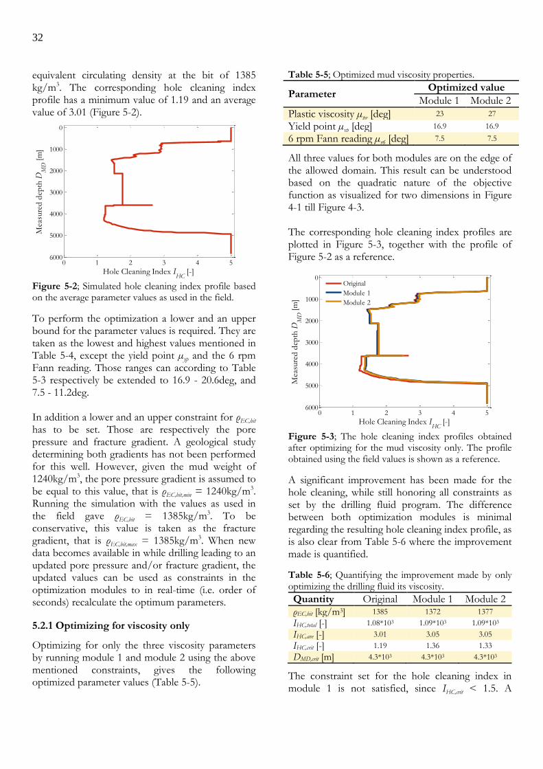
32

equivalent circulating density at the bit of 1385 kg/m3. The corresponding hole cleaning index profile has a minimum value of 1.19 and an average value of 3.01 (Figure 5-2).

Figure 5-2; Simulated hole cleaning index profile based on the average parameter values as used in the field.

To perform the optimization a lower and an upper bound for the parameter values is required. They are taken as the lowest and highest values mentioned in Table 5-4, except the yield point µyp and the 6 rpm Fann reading. Those ranges can according to Table 5-3 respectively be extended to 16.9 - 20.6deg, and 7.5 - 11.2deg. In addition a lower and an upper constraint for ρEC,bit has to be set. Those are respectively the pore pressure and fracture gradient. A geological study determining both gradients has not been performed for this well. However, given the mud weight of 1240kg/m3, the pore pressure gradient is assumed to be equal to this value, that is ρEC,bit,min = 1240kg/m3. Running the simulation with the values as used in the field gave ρEC,bit = 1385kg/m3. To be conservative, this value is taken as the fracture gradient, that is ρEC,bit,max = 1385kg/m3. When new data becomes available in while drilling leading to an updated pore pressure and/or fracture gradient, the updated values can be used as constraints in the optimization modules to in real-time (i.e. order of seconds) recalculate the optimum parameters.

5.2.1 Optimizing for viscosity only

Optimizing for only the three viscosity parameters by running module 1 and module 2 using the above mentioned constraints, gives the following optimized parameter values (Table 5-5).

Table 5-5; Optimized mud viscosity properties.

Parameter Optimized value

Module 1 Module 2

Plastic viscosity µpv [deg] 23 27



All three values for both modules are on the edge of the allowed domain. This result can be understood based on the quadratic nature of the objective function as visualized for two dimensions in Figure 4-1 till Figure 4-3. The corresponding hole cleaning index profiles are plotted in Figure 5-3, together with the profile of Figure 5-2 as a reference.

Figure 5-3; The hole cleaning index profiles obtained after optimizing for the mud viscosity only. The profile obtained using the field values is shown as a reference.

A significant improvement has been made for the hole cleaning, while still honoring all constraints as set by the drilling fluid program. The difference between both optimization modules is minimal regarding the resulting hole cleaning index profile, as is also clear from Table 5-6 where the improvement made is quantified.

Table 5-6; Quantifying the improvement made by only optimizing the drilling fluid its viscosity.

Quantity Original Module 1 Module 2 ρEC,bit [kg/m3] 1385 1372 1377

IHC,total [-] 1.08*103 1.09*103 1.09*103

IHC,ave [-] 3.01 3.05 3.05

IHC,crit [-] 1.19 1.36 1.33

DMD,crit [m] 4.3*103 4.3*103 4.3*103

The constraint set for the hole cleaning index in module 1 is not satisfied, since IHC,crit < 1.5. A

0 1 2 3 4 5

0

1000

2000

3000

4000

5000

6000


[-]

Mea

sure

d d

epth

DM

D [

m]

0 1 2 3 4 5

0

1000

2000

3000

4000

5000

6000


[-]

Mea

sure

d d

epth

DM

D [

m]

Original

Module 1

Module 2

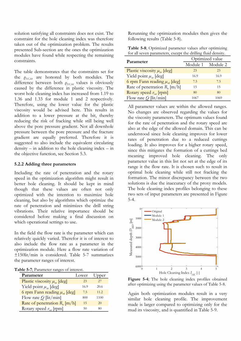
solution satisfying all constraints does not exist. The constraint for the hole cleaning index was therefore taken out of the optimization problem. The results presented Sub-section are the ones the optimization modules have found while respecting the remaining constraints. The table demonstrates that the constraints set for the ρEC,bit are honored by both modules. The difference between both ρEC,bit values is obviously caused by the difference in plastic viscosity. The worst hole cleaning index has increased from 1.19 to 1.36 and 1.33 for module 1 and 2 respectively. Therefore, using the lower value for the plastic viscosity would be advised here. This results in addition to a lower pressure at the bit, thereby reducing the risk of fracking while still being well above the pore pressure gradient. Not all downhole pressure between the pore pressure and the fracture gradient are equally preferred. Therefore it is suggested to also include the equivalent circulating density – in addition to the hole cleaning index – in the objective function, see Section 5.3.

5.2.2 Adding three parameters

Including the rate of penetration and the rotary speed in the optimization algorithm might result in better hole cleaning. It should be kept in mind though that these values are often not only optimized with the intention to maximize hole cleaning, but also by algorithms which optimize the rate of penetration and minimizes the drill string vibrations. Their relative importance should be considered before making a final discussion on which operational settings to use. In the field the flow rate is the parameter which can relatively quickly varied. Therefor it is of interest to also include the flow rate as a parameter in the optimization module. Here a flow rate variation of ±150lit/min is considered. Table 5-7 summarizes the parameter ranges of interest.

Table 5-7; Parameter ranges of interest.

Parameter Lower Upper




Flow rate Q [lit/min] 800 1100

Rate of penetration Rp [m/h] 15 20

Rotary speed vrot [rpm] 50 80

Rerunning the optimization modules then gives the following results (Table 5-8).

Table 5-8; Optimized parameter values after optimizing for all seven parameters, except the drilling fluid density.


Module 1 Module 2




Rate of penetration Rp [m/h] 15 15

Rotary speed vrot [rpm] 80 80

Flow rate Q [lit/min] 1067 1069

All parameter values are within the allowed ranges. No changes are observed regarding the values for the viscosity parameters. The optimum values found for the rate of penetration and the rotary speed are also at the edge of the allowed domain. This can be understood since hole cleaning improves for lower rates of penetration due to a reduced cuttings loading. It also improves for a higher rotary speed, since this mitigates the formation of a cuttings bed meaning improved hole cleaning. The only parameter value in this list not set at the edge of its range it the flow rate. It is chosen such to result in optimal hole cleaning while still not fracking the formation. The minor discrepancy between the two solutions is due the inaccuracy of the proxy models. The hole cleaning index profiles belonging to these two sets of input parameters are presented in Figure 5-4.

Figure 5-4; The hole cleaning index profiles obtained after optimizing using the parameter values of Table 5-8.

Again both optimization modules result in a very similar hole cleaning profile. The improvement made is larger compared to optimizing only for the mud its viscosity, and is quantified in Table 5-9.

0 1 2 3 4 5

0

1000

2000

3000

4000

5000

6000


[-]

Mea

sure

d d

epth

DM

D [

m]

Original

Module 1

Module 2

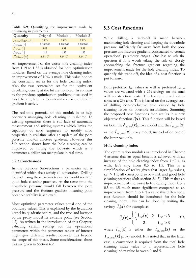
34

32

32ˆ3

4~

1

HC

HCHC

I

IIJ

xx

Table 5-9; Quantifying the improvement made by optimizing six parameters.

Quantity Original Module 1 Module 2 ρEC,bit [kg/m3] 1385 1385 1385

IHC,total [-] 1.08*103 1.18*103 1.18*103

IHC,ave [-] 3.01 3.31 3.31

IHC,crit [-] 1.19 1.55 1.55

DMD,crit [m] 4.3*103 3.6*103 3.6*103

An improvement of the worst hole cleaning index from 1.19 to 1.55 is obtained for both optimization modules. Based on the average hole cleaning index, an improvement of 10% is made. This value honors the constraint set in for the hole cleaning index. Also the two constraints set for the equivalent circulating density at the bit are honored. In contrast to the previous optimization problems discussed in this Chapter, here the constraint set for the fracture gradient is active. The real-time potential of this module is to help operators managing hole cleaning in real-time. In existing operations there is still lack of automatic measurement and mixing systems which limits the capability of mud engineers to modify mud properties in real-time after an update of the pore pressure and/or fracture gradient. However this Sub-section shows how the hole cleaning can be improved by tuning the flowrate which is a parameter a driller can manipulate in real-time.

5.2.3 Conclusions

In the previous Sub-sections a parameter set is identified which does satisfy all constraints. Drilling the well using these parameter values would result in good hole cleaning practices. At the same time the downhole pressure would fall between the pore pressure and the fracture gradient meaning good borehole stability is achieved. Most optimized parameter values equal one of the boundary values. This is explained by the hydraulics kernel its quadratic nature, and the type and location of the proxy model its extreme point (see Section 4.2). As written in the introduction of this Chapter, valuating certain settings for the operational parameters within the parameter ranges of interest might give different results, however this beyond the scope of this thesis. Some considerations about this are given in Section 6.2.

5.3 Cost functions

While drilling a trade-off is made between maximizing hole cleaning and keeping the downhole pressure sufficiently far away from both the pore pressure and fracture gradient, constrained to certain operational parameter ranges. One has to ask the question if it is worth taking the risk of closely approaching the fracture gradient regarding the improvement made for the hole cleaning index. To quantify this trade-off, the idea of a cost function is put forward. Both preferred IHC values as well as preferred ρEC,bit values are valuated with a 2% savings on the total well construction costs. The least preferred values come at a 2% cost. This is based on the average cost of drilling non-productive time caused by hole cleaning issues or borehole instabilities. Summing the proposed cost functions then results in a new

objective function xJ . This function will be based

on both the xbitEC , proxy model and the xcritHCI ,ˆ

or the xtotalHCI ,ˆ proxy model, instead of on one of

the latter two only.

Hole cleaning index

The optimization modules as introduced in Chapter 4 assume that an equal benefit is achieved with an increase of the hole cleaning index from 3 till 4, as with, let’s say, from 0.5 to 1.5. This is a simplification of reality given that larger IHC values, i.e. > 1.5, all correspond to low risk and good hole cleaning practices (Sub-section 2.1.3). This makes an improvement of the worst hole cleaning index from 0.5 to 1.5 much more significant compared to an improvement from 3 to 4. To value this difference a cost function should be introduced for the hole cleaning index. This can be done by writing the

savings x1

~J for example as

5-3

where xHCI is either the xcritHCI ,ˆ or the

xtotalHCI ,ˆ proxy model. It is noted that in the latter

case, a conversion is required from the total hole cleaning index value to a representative hole cleaning index value between 0 and 5.

min,,max,,

min,,,

,

ˆˆ

bitECbitEC

bitECbitECN

bitEC

xx

2-

ˆ3.51

1+4/1ˆ2sin

,

,

2x

xx

N

bitEC

N

bitECJ

242.2ˆ59.1exp1

07.4~11

xxx

HCIJJ

xxx 21 JJJ tot

The non-differentiable function of Equation 5-3 can be approximate by

5-4

This function will be part of the new objective function. The above two equations are graphically shown in Figure 5-5.

Figure 5-5; Cost function for the hole cleaning index IHC.

The graph for x1

~J shows that a hole cleaning index

of zero comes at a loss of 2% compared to the ‘base case’, when an hole cleaning index of 1.5 is achieved. For a hole cleaning index of zero, two percent more time is required to deliver the well due to required additional circulating time. For improvements of the hole cleaning index above 3 savings of 2% are made, meaning no additional value is created by increasing the hole cleaning index from 3 to 5.

Equivalent circulating density

The optimization modules as introduced in Chapter 4 also assume an equal cost of having a downhole pressure anywhere between the pore pressure and the fracture gradient. The optimization module ended up a few times at the fracture gradient (see for example Table 4-2 and Table 5-9). In the field one wants to refrain from approaching this gradient. Neither one wants to approach the pore pressure gradient. The equivalent circulating density at the bit should preferably be located as far away from both gradients as possible, while being shifted more towards the pore pressure gradient. To value this difference a cost function should also be introduced

for the equivalent circulating density. This can be

done by writing the savings x2J for example as

5-5

where N

bitEC , is the normalized proxy model for the

equivalent circulating density at the bit, defined as

5-6

Equation 5-5 is graphically shown in Figure 5-6.

Figure 5-6; Cost function for the normalized equivalent

circulating density at the bit N

bitEC , .

It shows that a money loss of 2% is associated with the downhole pressure when ρEC,bit is too low or too high. Ideally the downhole pressure is located

around N

bitEC , = 0.37, which saves 2% of time.

New objective function

Having identified a cost function for both the hole

cleaning index, x1J , as well as for the equivalent

circulating density, x2J , the total savings xtotJ

are now calculated as a function of the xHCI and

the xbitEC , proxy model via

5-7

This expression is the new objective function. Based on the proxy model for the worst hole

cleaning index, xcritHCI ,ˆ , the complete optimization

problem to be solved can now be stated as:

0 1 2 3 4 5

-2

-1.5

-1

-0.5

0

0.5

1

1.5

2


[-]

Sav

ings

J1 [

%]

J1

J1

~

0 0.2 0.4 0.6 0.8 1

-2

-1.5

-1

-0.5

0

0.5

1

1.5

2

Normalized equivalent circulating density at bit NEC,bit

[-]

Sav

ings

J2 [

%]

36

The functions for xcritHCI ,ˆ and xbitEC , are again

as given by Equation 3-8. In the optimization problem discussed in Sub-section 5.2.2 a worst hole cleaning index of 1.55 was found, and the equivalent circulating density at the bit equaled the chosen fracture gradient of 1385kg/m3. Here a less conservative fracture gradient of 1485kg/m3 it is assumed. Then, repeating this optimization problem with the

objective function as given by Equation 5-7 gives

%4.1xtotJ . The corresponding optimal

operational parameters are given in Table 5-10.

Table 5-10; Optimized parameter values when using the new objective function.


Plastic viscosity µpv [deg] 23

Yield point µyp [deg] 16.9

6 rpm Fann reading µr6 [deg] 7.5

Rate of penetration Rp [m/h] 15

Rotary speed vrot [rpm] 80

Flow rate [lit/min] 1100

Compared to the optimized values found in Table 5-8 only the flow rate has increased to its maximum value, resulting in ρEC,bit = 1388kg/m3, in an optimized IHC,crit value of 2.12, and in a worst hole cleaning index along the optimized profile of 1.58. This result can now quantified and reflected upon based on the introduced cost functions.

Visualization of the new objective function

The optimization problem solved above can be visualized by running optimization module 1 multiple times, by imposing each time a different downhole pressure falling between the pore pressure and the fracture gradient. Here this is done 8 times, and in that way 8 optimal hole cleaning index profiles are obtained. Below the optimized IHC,crit is

plotted versus N

bitEC , . The range covered by N

bitEC ,

corresponds with the range that can be reached with the current parameter ranges of interest (Table 5-7).

Figure 5-7; Optimized IHC,crit as a function of N

bitEC , .

The red dots are the data points, and the dashed line connects them.

In combination with the cost functions, this graph gives the objective function dealt with by optimization module 3. Figure 5-8 plots J1(x), J2(x), and the new objective function Jtot(x).

Figure 5-8; Visualization of the objective function dealt with by optimization module 3.

0.48 0.5 0.52 0.54 0.56 0.58 0.61

1.2

1.4

1.6

1.8

2


[-]

Op

tim

ized

IH

C,cri

t [-]

0.48 0.5 0.52 0.54 0.56 0.58 0.6-1

-0.5

0

0.5

1

1.5

2


[-]

Sav

ings

J [

%]

J1 [%]

J2 [%]

Jtot

[%]


Maximize

xx

xxx

bitECcritHC

c

tot

JIJ

fJfJJ

,2,1

2211

ˆˆ

ˆˆ

Subject to

242.2ˆ59.1exp1

07.4

,

1

x

x

critHCIJ

5.1ˆˆmin.,,1 xxx critHCcritHC

c IIf

2-

ˆ3.51

1+4/1ˆ2sin

,

,

2x

xx

N

bitEC

N

bitECJ

min,,,2ˆˆ

bitECbitECf xx

max,,,2ˆˆ

bitECbitECf xx

U

ii

L

i xxx

Based on the introduced cost functions, these three graphs indeed visualize that the improvements made on the hole cleaning index are valuable enough to compensate the reduction in savings made by increasing ρEC,bit all the way up to the maximum value that can be reached while still honoring the given parameter ranges.

Other representatives of the hole cleaning index

The hole cleaning index can also be represented by for example the average hole cleaning index by using

the xtotalHCI ,ˆ proxy model in optimization module 3

instead of the xcritHCI ,ˆ proxy model. One could

also consider the worst hole cleaning index encountered along an optimized profile. This approach is shortly presented below based on the same data as used in Figure 5-7. For this purpose, the worst hole cleaning index encountered along the 8 optimized hole cleaning

index profiles is below plotted versus N

bitEC , .

Figure 5-9; The worst hole cleaning index encountered along the optimized hole cleaning index profile as a

function of N

bitEC , .

It is noted that this optimization approach does require the curve plotted above, since no proxy model for the worst hole cleaning index of the optimized profile exists to directly use as an objective function. This in contrast to the case when one uses the optimized IHC,crit or the optimized IHC,total as a representative for the hole cleaning index, for which in both cases a proxy model does exist.

In combination with the cost functions, the graph of Figure 5-9 gives a different objective function. In Figure 5-10 J1(x), J2(x), and Jtot(x) are plotted.

Figure 5-10; The result expressed in profit of optimizing for the combined effect of hole cleaning and downhole pressure.

The improvements made on the hole cleaning index are not sufficient to compensate the reduction in savings made by increasing ρEC,bit all the way up to the maximum value that can be reached while still honoring the given parameter ranges. There is a balance between improving the hole cleaning index and approaching the pore pressure or fracture gradient. Based on the criteria set here, the well is best drilled using a parameter combination resulting in ρEC,bit = 0.54, resulting in savings of +1%.

Conclusions

The results obtained here depend on the cost functions applied, the representative of the hole cleaning index selected, the parameter ranges of interest chosen, and the pore pressure and fracture gradient assumed. Still they probably lead to a more realistic view on what the optimum mud properties and operational parameters would be in a real field situation compared to not applying a cost function at all. Future research should be done to quantify the expected costs related to in- or decreasing the hole cleaning index at the expense of approaching or moving away from the pore pressure/fracture gradient.

0.48 0.5 0.52 0.54 0.56 0.58 0.61

1.1

1.2

1.3

1.4

1.5

1.6


[-]

Wo

rst

IH

C a

lon

g o

pti

miz

ed p

rofi

le [

-]

0.48 0.5 0.52 0.54 0.56 0.58 0.6-1

-0.5

0

0.5

1

1.5

2


[-]

Sav

ings

J [

%]

J1 [%]

J2 [%]

Jtot

[%]

38


The envisioned workflow for the developed optimization module in combination with the borehole stability software is introduced. The added value of the developed optimization module became clear based on a case study. It is shown that significant improvements could have been made regarding hole cleaning when using the parameter values as determined by the developed optimization module, while still honouring the constraints as given by the drilling fluid program. This can potentially lead to faster delivery of a well, thereby saving costs.

To obtain a more realistic view on the added value of maximizing hole cleaning, the idea of a cost function is put forward. For both the hole cleaning index as well as the equivalent circulating density a mathematical formulation of what a cost function for both these quantities might look like in a real field situation is introduced. Both cost functions significantly influence the values found for the optimum operational parameters, and should hence be chosen with care. Future research is required to derive cost functions applicable to a to-be-drilled well. Those can subsequently combined with the here developed optimization module to find the optimal mud specifications and operational parameters.

Chapter 6

6Conclusions and recommendations

6.1 Conclusions

In this thesis, the design and implementation of an algorithm to automatically find drilling fluid properties and optimal operational settings given certain constraints has been considered. The mitigation of non-optimal drilling fluid properties and/or operational settings is of great practical interest because they might lead to borehole instabilities and to a reduced hole cleaning efficiency, resulting in increased safety risks and costly drilling non-productive time. The objective of this thesis (as stated in Chapter 1) is the development of an optimization module, based on an existing hydraulics kernel, that systematically derives the optimal drilling fluid properties and operational settings, in the sense that they maximize the hole cleaning index while maintaining borehole stability. The developed tool could help engineers plan their drilling fluid programs more scientifically, i.e., compared to the current practice. A set of optimization modules is devised that requires users to only define the ranges of interest for the input parameters to be optimized, and fixed parameters such as the well geometry, and the pore pressure and fracture gradient. The procedure will:

automatically derive proxy models for the hole cleaning index and the equivalent circulating density that are used in an optimization framework;

check the derived models for their accuracy based on four proposed criteria;

run the selected optimization module giving the optimum mud properties and/or operational parameters as an output.

Second-order polynomial regression models proved to be adequate as a basis for the proxy models since they capture the input/output structure of the hydraulics kernel sufficiently within a given subspace. Three optimization modules are considered is this work taking as objective function:

The worst hole cleaning index encountered along a profile.

The summed hole cleaning index profile.

A cost function containing both the hole cleaning index as well as the equivalent circulating density.

An exhaustive search approach was added to each optimization module to ensure that the optimal parameter values found by the sequential quadratic programming algorithm are indeed optimal. The speed of each optimization module (in the order of seconds) would allow users to recalculate the optimum operational parameters in real-time after a potential update of the borehole stability model or fracture gradient. It should be kept in mind though that the hydraulics kernel is a static model not taking into account cuttings which built up in the past. The differences between the optimum values computed using the first two objective functions, i.e., maximizing the worst hole cleaning index and maximizing the summed hole cleaning index turned out to be very limited in the case study investigated in this thesis, making both objective functions equally valid. Implementation of these optimization

40

modules on the case study demonstrated the potential of the module, since a significant improvement of 10% was made while still being confined to the parameters ranges as used in the field. To prevent small increases in the hole cleaning index at the expense of a significant step towards the pore pressure or fracture gradient, the concept of a cost function, depending on hole cleaning as well as on downhole pressure, is introduced. Depending on the shapes of cost functions included, the results obtained might significantly differ from the results obtained using an optimization module without cost functions. The proper selection of cost functions is therefore key in realizing a suitable advice on the optimal mud properties and/or operational parameters. In this work examples of what cost functions might look like have been given.

6.2 Recommendations

In this final Section, recommendations for future research and implementation purposes are given. In the scope of the workflow to derive proxy models, as introduced in Chapter 3, a second-order polynomial regression model proved to be adequate based on the introduced criteria. However, the regression coefficients determined and regression variables included in the model turned out to be different for every fit. While this did not significantly affect the accurate description of the kernel outputs, the Lagrangian of each model is different, potentially leading to a different optimum. Additional weighting of the data points on which the proxy model is built or averaging multiple models might mitigate the variation among the Lagrangians. Optimization of the drilling fluid properties has been done based on the hydraulics kernel only, meaning the resulting properties are optimum in the sense that they optimize the equivalent circulating density and/or the hole cleaning index. Compared to the field, the optimization problem considered here is subject to a limited set of constraints. In the field multiple other considerations are made and

limitations exist. It is recommended to formulate as many of them as possible in the form of a cost function, to mitigate the risks of implementing non-optimal drilling fluid properties. Those formulations should then be included as constraints in the optimization module as well. For example, in the field

a higher flow rate is more expensive, since the pumps wear more quickly. Or in general, the valuation of the parameter values within the selected ranges is taken into account;

one also wants to deliver a well as quickly as possible. Therefore, the rate of penetration is not simply set as low as possible as advised by the optimization modules;

the rotary speed of the drill string is not set as high as possible as advised by the optimization module, since next to maximizing hole cleaning, also drill string vibrations are mitigated;

the cuttings concentration built up in the past is taken into account. This is not done by the optimization module since it is a static calculation.

Regarding the outputs of the optimization module, the concept of a cost function as objective function was already put forward. To obtain a more solid advice on the optimum drilling fluid properties, it is recommended to for each well to be drilled to carefully quantify the cost of improving the hole cleaning index in terms of the associated change in the equivalent circulating density. To be able to implement the optimum mud properties as advised by the optimization module in the field, an accurate control of the mud properties is needed. It is therefore recommended to connect the optimization module to a real-time control system, which takes the setpoints as computed by the module as an input, and makes use of real-time mud measurement data and an automatic mud mixing system (Figure 1-2). Further gains could be made by improving the quality pore pressure and fracture gradient prediction. If costs allow, it is recommended to acquire input data for the borehole stability software more frequently.

41

nk 0

e

Appendix A

Rheology

This Appendix discusses the rheological properties of drilling fluids, the factors that influence these properties and the impact they have with respect to performing work during the drilling operation. Rheology is the science of deformation and flow of matter, and it is primarily concerned with the relationship between the shear stress τ experienced by a surface and the shear rate γ of the fluid exerting the shear stress. The shear stress is the force per unit area in N/m2 acting parallel to a surface. It is by definition perpendicular to the normal stress. The shear rate is the velocity change per unit distance in s-1. For drilling fluids the relation between shear stress and shear rate is given by the Herschel Bulkley model

A-1

Here τ0 [N/m2] is the yield stress, k [N/m2.sn] the consistency factor, and n [-] the flow index. For τ0 = 0, and n = 1 this equation describes the shear rate versus shear stress behaviour of a Newtonian fluid. The flow index n is in essence a measure of how non-Newtonian the fluid is. For a shear thinning fluid it is between 0 and 1, and for a shear thickening fluid it is bigger than one. The yield stress τ0 represents the shear stress τ required to overcome internal forces and to initiate fluid flow.

Viscosity

The effective viscosity µe of a fluid is a fluid its viscosity under specific conditions. These conditions include shear rate, pressure and temperature. For a constant pressure and temperature, the viscosity is defined as

A-2

Drilling fluids are shear thinning, meaning their viscosity decreases for increasing shear. In contrast to Newtonian fluids, their viscosity cannot be characterized by a single coefficient for a given temperature. The rheology of a drilling fluid has a major influence on the efficiency of cuttings transportation from the drill bit to the surface. Drilling fluids require low viscosities at high shear rates to release the cuttings on the shakers and to minimize frictional pressure losses at the bit, medium viscosities at medium shear rates to transport cuttings, and high viscosities at low shear rates to suspend cuttings and to prevent fluid loss. This is schematically depicted in

Figure A-1.

Figure A-1; Viscosity requirements of drilling fluids [22].

42

703.1

5114.0

300600 pv

6003002 yp

Gel strength

To suspend cuttings and weighting agent in the static period, drilling fluids form a gel when no shear is applied, and then become fluid again when shear is applied. Gelation should not be any stronger than needed to perform these functions. Gelation occurs due to linking of charged particles and/or polymers forming a rigid matrix. The gel formation should stop after a couple of minutes to prevent excessive gel strengths. Those are called non-progressive gels. This in contrast to progressive gels, which keep on increasing in strength as time continues. When coming from the factory, the mud is non-progressive. While drilling clay might be added to the mud when drilling a shale formation. This makes the drilling fluid more progressive. Correct removal of cuttings at the surface is essential to ensure that the mud remains non-progressive. A common way of breaking gels is to turn on the pumps. For high gel strengths this might lead to bursting the formation. In the case progressive gels one better uses mechanical power (turn the drill string) instead of hydraulic power (start up the pump).

Field measurements

In the field the viscosity is mostly measured offline using a Fann viscometer (Figure A-2).

Figure A-2; The Fann viscometer [3].

A mud sample is placed in the cup. The rotor spins at one of the six available rotary speeds, that is at 3, 6, 100, 200, 300 or 600 rotations per minute. Due to the fixed geometry of the viscometer the rotary speed ω is related to the shear rate via

A-3

The application of a shear rate on the fluid makes the bob deflect a certain angle θ indicated on the deflection dial. For the Fann viscometer this angle is related to the shear stress via

A-4

In this way six points, θ3, θ6, ect., on the shear stress curve are obtained. Fitting the data points with the Herschel Bulkley model gives the complete viscosity profile. In the field the mud viscosity is characterized by three parameters, the plastic viscosity, µpv, the yield point, µyp, and the 6rpm Fann reading µr6. Those are related to the Fann readings via

A-5

A-6

43

66 rA-7

In drilling fluid programs these three quantities are reported in standard oilfield units as lb/100ft2 instead of in degrees. The conversion factor from degrees to lb/100ft2 is 1.0678. Viscometer readings in degrees are often used as the shear stress in lb/100ft2 without this conversion since the difference is small. The plastic viscosity is a function of particle loading and should be controlled as low as possible. Any increase in the total surface area of solids exposed will be reflected in an increased plastic viscosity. The plastic viscosity is mainly affected by the size and shape of the solids and the solids concentration. An increase of the latter one can be verified by a density measurement. In the field one often targets a plastic viscosity as low as possible. The yield point is a measure for the attractive forces between particles in a fluid. These forces originate from electrical charges located on the particle surfaces. It is a measurement of the carrying capacity of the fluid under flowing conditions. The closer the particles move together the higher the yield point. A lot of particles which do not interact still give a yield point of zero, which means a Newtonian fluid.

45

Appendix B

BInput hydraulics software

The Hydraulics kernel has multiple inputs, but not all of them are of equally importance when it comes to the influence they have on the simulated profile pressure in a well. Theis et al identified that 95% of the variations observed in the simulated pressure profile can already be explained by variations in 19 well design and 12 operational parameters only [18]. See the list and Figure B-1 below: Well design parameters (19 in total):

Well Survey (direction) (4 parameters)

o Vertical depth

o Build length

o Hold length

o Hold angle

Well design properties (5 parameters)

o Open hole diameter

o Casing inner diameter

o Casing shoe depth

o Formation temperature gradient

o Formation surface temperature

Drill string properties (10 parameters)

o Bit total flow area

o Length of drill pipe single

o Length of drill pipe tooljoint

o Outer diameter of pipe body

o Inner diameter of pipe body

o Outer diameter of pipe tooljoint

o Inner diameter of pipe tooljoint

o Length of bottom hole assembly

o Outer diameter of bottom hole assembly

o Inner diameter of bottom hole assembly

Operational parameters (12 in total):

Fluid properties (7 parameters)

o Mud density

o Mud reference temperature

o Low gravity solids %

o Low gravity solids density

o Herschel-Bulkley 𝜏𝑦

o Herschel-Bulkley 𝑘

o Herschel-Bulkley 𝑛

Operational conditions (5 parameters)

46

o Flow rate

o Rate of penetration

o String rotary speed

o Cuttings density

o Cuttings size

Figure B-1; Schematic explanation of the parameters listed above. Note the following abbreviations: OD - outer diameter; ID - inner diameter; BHA - bottom hole assembly [18].

47

Appendix C

CValues of input parameters

The improvements that could have been made by applying the developed automatic setpoint search algorithm are quantified in Chapter 5 based on two case studies. The values of all the fixed input parameters required by the kernel are summarized below for both case studies.

Case study I

The well trajectory is presented in Figure C-1. The well contains a 23’’, 12¼’’, 8½’’, and 6’’ hole section, which are respectively cased off by a 20’’ casing, a 9⅝’’ casing, a 7’’ liner, and a 3½’’ liner. Further geometry features are not provided here, neither are the dimensions of the drill string included. Figure C-2 shows the temperature profile along the well.

Figure C-1; The well trajectory.

Figure C-2; The temperature profile.

0 500 1000 1500 2000 2500

0

500

1000

1500

2000

2500

3000

3500

4000

Outstep [m]

Tru

e ver

tica

l d

epth

D [

m]

Well trajectory Case study II

260 280 300 320 340 360 380 400 420

0

1000

2000

3000

4000

5000

Temperature T [K]

Mea

sure

d d

epth

DM

D [

m]

Temperature profile Case study II

48

Table C-1 includes the values of the remaining fixed input parameters. The average values of the parameters which can be included in a proxy model are for completeness also included in this Appendix (Table C-2).

Table C-1; Values of all fixed input parameters as required by the kernel except borehole geometry, drill string geometry and temperature profile.

Parameter Value

Weight on bit [N] 12000

Cuttings density [kg/m3] 2600

Cuttings diameter [m] 6.35*10-3

Cuttings bed porosity [%] 37

Hole measured depth [m] 4778

Bit measured depth [m] 4778

hydrInput.reamerPresent [-] 0

hydrInput.aqPct [-] 25

hydrInput.oilType [-] 201

hydrInput.loDen [kg/m3] 2650

hydrInput.hiDen [kg/m3] 4200

hydrInput.loDenPct [%] 0

hydrInput.mudRefTemp [K] 323.15

hydrInput.mudRefPres [Pa] 101353

hydrInput.brine.Nacl [%] 10

hydrInput.brine.KCl [%] 0

hydrInput.brine.CaCl2 [%] 0

hydrInput.brine.ZnCl2 [%] 0

hydrInput.brine.NaBr [%] 0

hydrInput.brine.KBr [%] 0

hydrInput.brine.CaBr2 [%] 0

hydrInput.brine.ZnBr2 [%] 0

hydrInput.surfaceBackPressure [Pa] 101325

hydrInput.drillStringRestriction [-] 0

hydrInput.epsilon [-] 0

hydrInput.cuttingsEnabled [-] 1

hydrInput.oldLamLookUp [-] 0

Table C-2; The average values of the operational parameters which can be included in a proxy model. The Fann readings from which µpv, µyp, and µr6 are calculated are included.

Parameter Value


Rate of penetration [m/h] 12

Rotary speed of drill string [rpm] 160

Mud weight [kg/m3] 1420

Plastic viscosity [deg] 24

Yield point [deg] 33

6rpm Fann reading [deg] 10

Fann reading θ600 [deg] 81






49

Case study II

The well trajectory is presented in Figure C-3. The well contains a 23’’, 17½’’, 12¼’’, 8½’’, and 6’’ hole section, which are respectively cased off by a 18⅝’’ casing, a 13⅜’’ casing, a 9⅝’’ casing, a 7’’ liner, and a 5’’ liner. Details

are summarized in Table C-3. The dimensions of the drill strings used to drilled the separate well sections are not included in this thesis. Figure C-4 shows the temperature profile along the well.

Figure C-3; The well trajectory.

Table C-3; Geometry of the well.

Section Measured depth DMD [m] True vertical depth D [m]

23’’ 652 617

17½’’ 1362 1116

12¼’’ 3739 1933

8½’’ 5546 3122

6’’ 5846 3405

Figure C-4; The temperature profile.

Table C-4 includes the values of the remaining fixed input parameters. The average values of the parameters which can be included in a proxy model are for completeness also included in this Appendix (Table C-5). The Fann readings from which the plastic viscosity, µpv, the yield point, µyp, and the 6rpm Fann reading, µr6, are calculated are also mentioned.

01000

20003000

4000 -2000

0

2000

4000

0

1000

2000

3000

4000

y-coordinate [m]

Well trajectory Case study I

x-coordinate [m]

Tru

e ver

tica

l d

epth

D [

m]

260 280 300 320 340 360 380 400 420

0

1000

2000

3000

4000

5000

6000

Temperature T [K]

Mea

sure

d d

epth

DM

D [

m]

Temperature profile Case study I

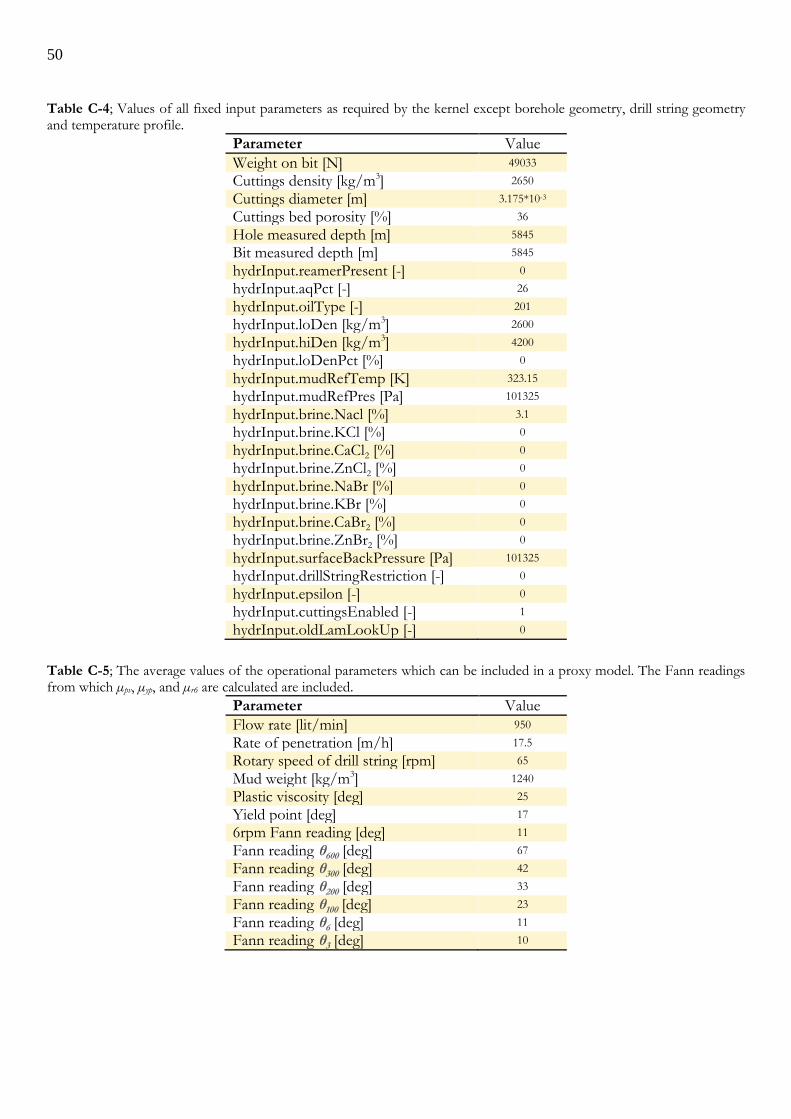
50

Table C-4; Values of all fixed input parameters as required by the kernel except borehole geometry, drill string geometry and temperature profile.

Parameter Value

Weight on bit [N] 49033

Cuttings density [kg/m3] 2650

Cuttings diameter [m] 3.175*10-3

Cuttings bed porosity [%] 36

Hole measured depth [m] 5845

Bit measured depth [m] 5845

hydrInput.reamerPresent [-] 0

hydrInput.aqPct [-] 26

hydrInput.oilType [-] 201

hydrInput.loDen [kg/m3] 2600

hydrInput.hiDen [kg/m3] 4200

hydrInput.loDenPct [%] 0

hydrInput.mudRefTemp [K] 323.15

hydrInput.mudRefPres [Pa] 101325

hydrInput.brine.Nacl [%] 3.1

hydrInput.brine.KCl [%] 0

hydrInput.brine.CaCl2 [%] 0

hydrInput.brine.ZnCl2 [%] 0

hydrInput.brine.NaBr [%] 0

hydrInput.brine.KBr [%] 0

hydrInput.brine.CaBr2 [%] 0

hydrInput.brine.ZnBr2 [%] 0

hydrInput.surfaceBackPressure [Pa] 101325

hydrInput.drillStringRestriction [-] 0

hydrInput.epsilon [-] 0

hydrInput.cuttingsEnabled [-] 1

hydrInput.oldLamLookUp [-] 0

Table C-5; The average values of the operational parameters which can be included in a proxy model. The Fann readings from which µpv, µyp, and µr6 are calculated are included.

Parameter Value


Rate of penetration [m/h] 17.5

Rotary speed of drill string [rpm] 65

Mud weight [kg/m3] 1240

Plastic viscosity [deg] 25

Yield point [deg] 17

6rpm Fann reading [deg] 11







51

Appendix D

DExtended range sensitivity

The behaviour and sensitivity of the kernel its output on the selected input parameters was investigated by varying those parameters one by one over a range of 20%. The simulated equivalent circulating density and average hole cleaning index were plotted in Figure 2-5, and it was observed that all responses were smooth. In contrast to 20%, here the parameter values are varied over a larger range of 50%. The simulated equivalent circulating density and average hole cleaning index are plotted in Figure D-1.

Figure D-1; Visualization of the behavior and sensitivity of a) the equivalent circulating density at the bit and b) the average hole cleaning index on applying a 50% variation on one input parameter at a time.

The responses demonstrate – albeit only in one dimension – the non-linear behaviour of the kernel. They are significantly less smooth compared to the responses plotted in Figure 2-5. Accurately describing this behaviour with a proxy model would require a more complex formulation, and the linear regression model as introduced by Equation 3-8 would not suffice. Considering the variation of multiple parameters simultaneously could introduce even stronger non-linear behaviours in the response variables due to possible interactions among the parameters. The analysis presented in this Appendix proves that a suitable range for all dimensions has to be chosen when building a proxy model based on a given equation.

50 100 150

1360

1370

1380

1390

1400

1410

1420

1430

Parameter variation [%]Equiv

alen

t ci

rcula

tin

g d

ensi

ty a

t b

it

EC

,bit [

kg/

m3]

50 100 150

900

1000

1100

1200

1300

1400

1500

1600

1700

1800

1900

a)50 100 150

2.9

2.95

3

3.05

3.1

3.15

3.2


Aver

age

ho

le c

lean

ing

ind

ex I

HC

,ave

[-]

50 100 150

2.5

3

3.5

4

b)80 85 90 95 100 105 110 115 120

1100

1200

1300

1400

1500

1600

1700


Equiv

ale

nt

circula

ting d

ensity a

t th

e b

it

EC

,bit [

kg/m

3]

Flow rate Q (right axis)


Rotatry speed vrot

Mud weight df


Yield point yp


80 85 90 95 100 105 110 115 1201100

1200

1300

1400

1500

1600

1700


Equiv

ale

nt

circula

ting d

ensity a

t th

e b

it

EC

,bit [

kg/m

3]

Flow rate Q (right axis)


Rotatry speed vrot

Mud weight df


Yield point yp


53

k

levelsFFD nN

Appendix E

EDesign of experiments

In this thesis proxy models are fitted to a subspace of the hydraulics kernel. This subspace is defined by the input parameters of interest, the corresponding ranges of interest, and the output parameters of interest (Section 2.1 and 2.2). Within this subspace data has to be collected from the kernel to which subsequently a proxy model can be fitted. Proxy models should be created as accurately and quickly as possible, meaning one should carefully consider in which data points to sample the output. Various techniques – or design of experiments – exist to sample a k-dimensional space.

Full factorial design

Full factorial design includes all possible states of the system. The number of sample taken, NFFD, is given by

E-1

where k is the number of input parameters, and nlevels the number of levels included in the design. Including five parameters in the proxy model, while calculating the output for ten levels (i.e. values) of each input parameter results in NFFD = 105. Since the simulation time of kernel is over one second per calculation, this design technique takes a lot of time. More efficient designs are the random design and the latin hypercube design.

Random design

In a random design the data points are distributed randomly throughout the k-dimensional space. This creates areas of dense and areas of sparse coverage. This is unwanted, since a proxy models might become inaccurate in areas of sparse coverage. In addition, relatively dense coverage reduces the amount of information contained per sample and is hence an unnecessary cost. As an example consider a 2-dimensional random design consisting of NRD = 100 samples. A graphical representation of it is shown in Figure E-1. Both parameters can take values between 0 and 1.

Figure E-1; Two dimensional random design consisting of 100 samples. Both parameters vary between zero and one.

0 0.2 0.4 0.6 0.8 10

0.2

0.4

0.6

0.8

1

Parameter 1 [-]

Par

amet

er 2

[-]

Random design

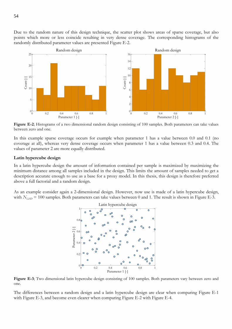
54

Due to the random nature of this design technique, the scatter plot shows areas of sparse coverage, but also points which more or less coincide resulting in very dense coverage. The corresponding histograms of the randomly distributed parameter values are presented Figure E-2.

Figure E-2; Histograms of a two dimensional random design consisting of 100 samples. Both parameters can take values between zero and one.

In this example sparse coverage occurs for example when parameter 1 has a value between 0.0 and 0.1 (no coverage at all), whereas very dense coverage occurs when parameter 1 has a value between 0.3 and 0.4. The values of parameter 2 are more equally distributed.

Latin hypercube design

In a latin hypercube design the amount of information contained per sample is maximized by maximizing the minimum distance among all samples included in the design. This limits the amount of samples needed to get a description accurate enough to use as a base for a proxy model. In this thesis, this design is therefore preferred above a full factorial and a random design. As an example consider again a 2-dimensional design. However, now use is made of a latin hypercube design, with NLHD = 100 samples. Both parameters can take values between 0 and 1. The result is shown in Figure E-3.

Figure E-3; Two dimensional latin hypercube design consisting of 100 samples. Both parameters vary between zero and one.

The differences between a random design and a latin hypercube design are clear when comparing Figure E-1 with Figure E-3, and become even clearer when comparing Figure E-2 with Figure E-4.

0 0.2 0.4 0.6 0.8 10

5

10

15

20

25

Parameter 1 [-]

Co

un

t [-

]

Random design

0 0.2 0.4 0.6 0.8 10

2

4

6

8

10

12

14

16

Parameter 2 [-]

Co

un

t [-

]

Random design

0 0.2 0.4 0.6 0.8 10

0.2

0.4

0.6

0.8

1

Parameter 1 [-]

Par

amet

er 2

[-]


55

Figure E-4; Histograms of a two dimensional latin hypercube design consisting of 100 samples. Both parameters can take values between zero and one.

The above histograms show an equal distribution of the parameter values over the entire multi-dimensional space covered by the parameters. This maximizes the amount of information contained per sample, thereby reducing the amount of samples needed to obtain an accurate representation of the kernel. This makes the latin hypercube design a suitable candidate for sampling the hydraulics kernel.

0 0.2 0.4 0.6 0.8 10

2

4

6

8

10

12

Parameter 1 [-]

Co

un

t [-

]Latin hypercube design

0 0.2 0.4 0.6 0.8 10

2

4

6

8

10

12

Parameter 2 [-]

Co

un

t [-

]


57

1

0

1212

0

1212

21

21

21

1

21

1

1

,,

dttt

dttt

xF

x

x

2

2

11

22

2

1

21

21

21

1

1

1

2,

2B

1,,

xxxf

1

0

11 1,B dtttyxyx

1121 pp

22 pN

Appendix F

FThe p-value

In Matlab, a p-value for a certain term is calculated using the F-distribution which is given by [27]

F-1

for real x ≥ 0. Here B is the beta function given by

F-2

and the number of degrees of freedom ν1 and ν2 are respectively given by

F-3

F-4

where N is the number of data points, and p1 and p2 are the amount of regression coefficients included in the more restricted model 1 and the less restricted model 2 respectively. For a few combinations of ν1 and ν2 the probability density function of the F-distribution is plotted below

Figure F-1; Probability density function for several combinations of ν 1 and ν 2.

The corresponding cumulative distribution function is given by

F-5

0 0.5 1 1.5 2 2.5 30

0.5

1

1.5

2

x

f(x

,1,

2)

F-distribution

1 = 1,

2 = 1

1 = 2,

2 = 1

1 = 5,

2 = 2

1 = 10,

2 = 1

1 = 50,

2 = 50

58

1

ˆ

ˆ

1

2

2,

1

2

1,

1

2

N

i

ii

N

i

ii

stat

yy

yy

F

21,,1value_ xFp

Here, x is the so called F-statistic of the problem which approaches 1 in the limit that x goes to infinity. The F-statistic is given by

F-6

where yi are the observed y-values by the kernel simulation, ŷi,1 and ŷi,2 the y-values as predicted by model 1 and model 2 respectively. Hence, the calculation of an F-statistic requires fitting with both models. Fitting is performed using the least square method which minimizes the residual square sum by varying the regression coefficients of the model. The p-value of a certain term is now be calculated via

F-7

To conclude, for step 2 this means that if the p-value of certain term is the smallest of all calculated p-values, the corresponding regressor is included in the proxy model, provided that it is smaller than the entrance criteria of 0.05. For step 3 this means that if the p-value of certain term is the biggest of all calculated p-values, the corresponding regressor is removed from the proxy model, provided that it is bigger than the exit criteria of 0.10.

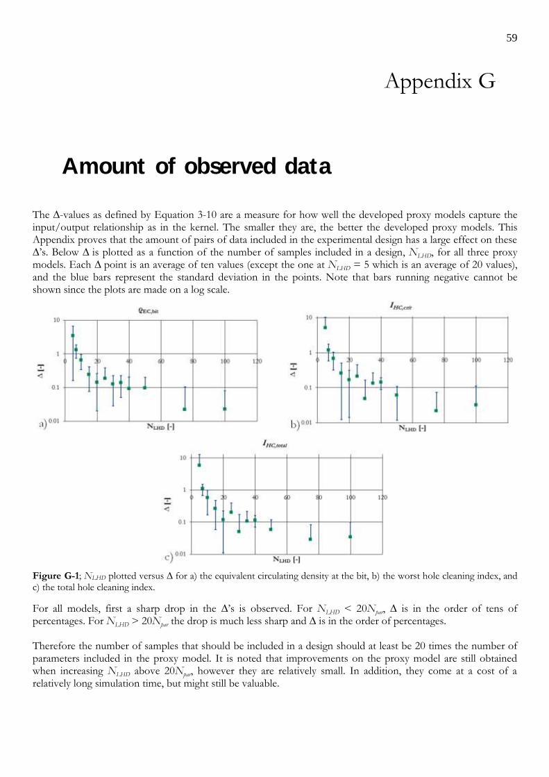
59

Appendix G

GAmount of observed data

The ∆-values as defined by Equation 3-10 are a measure for how well the developed proxy models capture the input/output relationship as in the kernel. The smaller they are, the better the developed proxy models. This Appendix proves that the amount of pairs of data included in the experimental design has a large effect on these ∆’s. Below ∆ is plotted as a function of the number of samples included in a design, NLHD, for all three proxy models. Each ∆ point is an average of ten values (except the one at NLHD = 5 which is an average of 20 values), and the blue bars represent the standard deviation in the points. Note that bars running negative cannot be shown since the plots are made on a log scale.

Figure G-1; NLHD plotted versus ∆ for a) the equivalent circulating density at the bit, b) the worst hole cleaning index, and c) the total hole cleaning index.

For all models, first a sharp drop in the ∆’s is observed. For NLHD < 20Npar, ∆ is in the order of tens of percentages. For NLHD > 20Npar the drop is much less sharp and ∆ is in the order of percentages. Therefore the number of samples that should be included in a design should at least be 20 times the number of parameters included in the proxy model. It is noted that improvements on the proxy model are still obtained when increasing NLHD above 20Npar, however they are relatively small. In addition, they come at a cost of a relatively long simulation time, but might still be valuable.

61

Appendix H

HSkewing

The issue of sparse coverage at high hole cleaning index values can partially be mitigated by skewing the distribution of flow rate input values towards higher flow rates, leading to more evenly distributed hole cleaning index values. To achieve skewing two transfer functions were introduced (Figure 3-7), redistributing the flow rate values within the covered range. The original distribution and the two skewed distributions are shown in the histograms below.

Figure H-1; a) The original flow rate distribution as created by the latin hyper cube design, b) The skewed flow rate distribution according to Qskewed = Q0.5, and c) The skewed flow rate distribution according to Qskewed = sin0.75(Qπ/2).

Preference is given to the sine function since it includes more high flow rate values as compared to the square root function. The resulting distributions of the values contained in the IHC,crit and IHC,total vector are shown in Figure H-2 and Figure H-3 respectively.

750 800 850 900 950 1000 1050 1100 11500

2

4

6

8

10

Flow rate [lit/min]

Fre

quen

cy [

-]

750 800 850 900 950 1000 1050 1100 11500

2

4

6

8

10

12

14

Flow rate [lit/min]

Fre

quen

cy [

-]

750 800 850 900 950 1000 1050 1100 11500

5

10

15

20

25

30

35

Flow rate [lit/min]

Fre

quen

cy [

-]

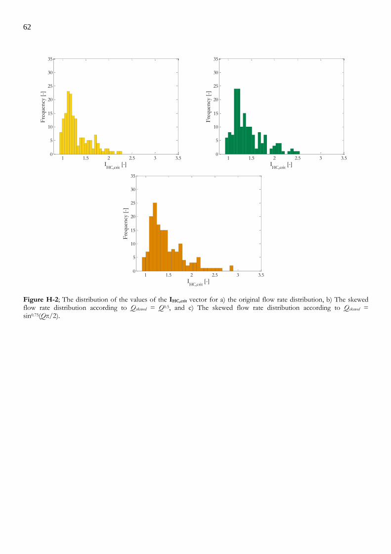
62

Figure H-2; The distribution of the values of the IHC,crit vector for a) the original flow rate distribution, b) The skewed flow rate distribution according to Qskewed = Q0.5, and c) The skewed flow rate distribution according to Qskewed = sin0.75(Qπ/2).

1 1.5 2 2.5 3 3.50

5

10

15

20

25

30

35

IHC,crit

[-]

Fre

quen

cy [

-]

1 1.5 2 2.5 3 3.50

5

10

15

20

25

30

35

IHC,crit

[-]

Fre

quen

cy [

-]

1 1.5 2 2.5 3 3.50

5

10

15

20

25

30

35

IHC,crit

[-]

Fre

quen

cy [

-]

63

Figure H-3; The distribution of the values of the IHC,total vector for a) the original flow rate distribution, b) The skewed flow rate distribution according to Qskewed = Q0.5, and c) The skewed flow rate distribution according to Qskewed = sin0.75(Qπ/2).

These Figures confirm that skewing the flow rate distribution results in a more evenly coverage, for both IHC,crit and IHC,total. Especially the coverage at the high end side of the distribution has improved. This has a positive effect on the residuals when making a fit, as was proven by Figure 3-8.

1000 1050 1100 1150 1200 1250 13000

5

10

15

20

25

IHC,total

[-]

Fre

quen

cy [

-]

1000 1050 1100 1150 1200 1250 13000

5

10

15

20

25

IHC,total

[-]

Fre

quen

cy [

-]

1000 1050 1100 1150 1200 1250 13000

5

10

15

20

25

IHC,total

[-]

Fre

quen

cy [

-]

65

0

x

x

x

xz

critHCHC

bitECbitEC

bitECbitEC

II ,min,

,min,,

max,,,

62015141295

19615131184

18614131073

17612111062

16698761

6,

,

,

,

,

,

2

2

2

2

2

ryppvdf

yprpvdf

pvrypdf

dfryppv

ryppvdf

rcritHC

ypcritHC

pvcritHC

dfcritHC

critHC

critHC

Q

Q

Q

Q

Q

I

I

I

I

QI

I

x

x

x

x

x

x

0

xz

λxJxλxL z

Ty,

Appendix I

IAnalytical description of optimization

problem

The solution to an optimization problem is the critical point of the so-called Lagrangian function L(x,λ) [28]. This critical point is calculated by equating the gradient of the Lagrangian function to the zero vector:

I-1

where ŷ is the objective function which has to be optimized by tuning the independent variables contained in the vector x. Further, J(x) is the Jacobian matrix of z(x), z(x) is the vector containing constraint functions, and λ is a vector with the same amount Lagrange multipliers as there are constraint functions. This equation is only valid for the active constraint functions. If a constraint is not active the concerning function will be smaller than zero. In this study the objective functions considered are IHC,crit(x) and IHC,total(x), the vector x contains (a selection of) the selected parameters as given in Section 2.2, and the optimization is constrained by three inequalities:

I-2

The functions included in these constraints are according to the general formulation as given by Equation 3-8, with their regression coefficients ß calculated via stepwise regression. They are non-linear functions, meaning the inequalities are non-linear too. For example, taking x = [Q ρdf µpv µyp µr6] we can write the gradient of the objective function ŷ(x) = IHC,crit(x) as

I-3

which is a vector of five linear functions.

66

6

,

66

,

,

,

,

r

critHC

r

EC

r

EC

yp

critHC

yp

EC

yp

EC

pv

critHC

pv

EC

pv

EC

df

critHC

df

EC

df

EC

critHCECEC

T

I

I

I

I

Q

I

QQ

xxx

xxx

xxx

xxx

xxx

xJ z

0

x

x

x

xx

xx

xx

xx

xx

λxL

critHCcritHC

bitECbitEC

bitECbitEC

r

EC

r

critHC

yp

EC

yp

critHC

pv

EC

pv

critHC

df

EC

df

critHC

ECcritHC

II

I

I

I

I

QQ

I

,min,,

,min,,

max,,,

5

6

4

6

,

54

,

54

,

54

,

54

,

,

Further, the Jacobian matrix of z(x) is given by

I-4

Then, substitution of the above three expressions in Equation I-1 with λ = [λ1 λ2 λ3]T results in

I-5

where λ4 = 1 - λ3 and λ5 = λ1 – λ2. Again, this equation is only valid for the active constraint functions. This is the mathematical formulation of the optimization problem which should be solved for the vector x by optimization module 1. A similar formulation can be given for the optimization problem which should solved by optimization

module 2. As shown by Equation I-3 the objective function alone, so without constraints, would have resulted a linear set of equations, solvable analytically. Due to the addition of non-linear constraints both optimization problems are non-linear, and cannot be solved analytically via Gauss Jordan elimination. Hence both optimization modules will make use of numerical techniques.

67

Bibliography

[1] “BaraLogix™ Real-Time & Automation Services,” Halliburton, [Online]. Available: http://www.halliburton.com/en-US/ps/baroid/real-time-services/baralogix.page.

[2] B. Bloys, N. Davis, B. Smolen, L. Bailey, O. Houwen, P. Reid, J. Sherwood, L. Fraser and M. Hodder, “Designing and Managing Drilling Fluid,” Oilfield Review, pp. 33-43, April 1994.

[3] T. Schuit, “Thesis: Control of drilling fluid properties; Density and Viscosity,” Shell, Rijswijk, 2015.

[4] R. Nafikov and M. Glomstad, “Automatic Mud Mixing,” in SPE-163473-MS, Amsterdam, 2013.

[5] J. Matheus, M. Ignova and P. Hornblower, “A Hybrid Approach to Closed-loop Directional Drilling Control using Rotary Steerable Systems,” Elsevier, vol. 45, no. 8, pp. 84-89, 2012.

[6] H. Melgares, W. Grace, F. Gonzalez, C. Alric, J. Palacio and G. Akinniranye, “Remote Automated Directional Drilling Through Rotary Steerable Systems,” in SPE-119761-MS, Amsterdam, 2009.

[7] T. Vromen, N. v. d. Wouw, A. Doris, P. Astrid and H. Nijmeijer, “Observer-based output-feedback control to eliminate torsional drillstring vibrations,” Proceedings of the IEEE Conference on Decision and Control, pp. 872-877, Febr 2015.

[8] W. Aldred, J. Bourque, M. Mannering, C. Chapman, B. d. Castel, R. Hansen, G. Downton, R. Harmer, I. Falconer, F. Florence, E. G. Zurita, C. Nieto, R. Stauder and M. Zamora, “Drilling Automation,” Oilfield Review, vol. 24, no. 2, pp. 18-27, 2012.

[9] Drilling Fluids Engineering Manual - Chapter 5, M-I, 1998.

[10] Wells Distance Learning Package, Volume 1, Section 4, Part 1, The Hague, The Netherlands: Shell International Exploration and Production B.V., 2005.

[11] A. Chan, “The STABOR User Companion,” Shell International Exploration and Production Inc., Houston, 2010.

[12] J. Wentink, “WellHydraulics NextGeneration Verification and Acceptance Report,” Shell Global Solutions International B.V., Rijswijk, 2014.

[13] J. Dudley, J. Nicholson, J.C.Woodhouse, M. Albrecht, S. Zeilinger, E. v. Oort and A. Tutuncu, “Borehole stability analysis prospect princess, Offshore Gulf of Mexico,” Shell Technology EP, Houston, 2000.

[14] A. Tutuncu, J. Nicholson, S. Zeilinger, E. V. Oort and Q. Sharif, “Borehole Stability Analysis Prospect Auger, Offshore Gulf of Mexico,” Shell Technology EP, Houston, 2001.

[15] L. van der Sluis, “Thesis: Design of an automatic drilling fluid measurement setup and closed loop pH control,” Shell, Rijswijk, 2012.

[16] J. Gunnerod, S. Serra, M. Palacios-Ticas and O. Kvarne, “Highly automated drilling fluids system improves HSE and efficiency, reduces personnel needs,” Drilling Contractor, vol. Jan/Febr, pp. 73-77, 2009.

[17] J.-D. Jansen, O. Bosgra and P. v. d. Hof, “Model-based control of multiphase flow in subsurface oil reserviors,” Journal of Process Control, vol. 18, pp. 846-855, 2008.

[18] W. Theis and J. Wentink, “Experimental Design to define sensitivity requirements for mud sensors,” Shell Global Solutions International, B.V., Rijswijk, 2015.

[19] Wells Distance Learning Package, Volume 2, Section 7, Part 1, The Hague, The Netherlands: Shell International Exploration and Production B.V., 2008.

[20] B. v. d. Brule and S. v. d. Marck, “Flow of generalised Newtonian fluids in conduits of arbitrary cross sectional shapes,” Goup Research Report, SIEP, 1994.

68

[21] I. Azouz, S. Shirazi, A. Pilehvari and J. Azar, “Numerical Simulation of Laminar Flow of Yield-Power_Law Fluids in Conduits of Arbitrary Cross-Section,” Journal of Fluids Engineering, vol. 115, pp. 710-716, 1993.

[22] SEPCO, “Hole cleaning best practices quick guide,” Shell EP, 2003.

[23] Wells Workbench Hydraulics manual, Shell International Ltd., 2015.

[24] N. Elshout, T. Barkmann, R. Mahrous, J. de Bruijn and S. Haan, “Mud Program Case Study II,” Baroid Drilling Fluids Design & Services Program, 2015.

[25] M. Westink, P. Rijnen and S. Roggeband, “Mud Program for Case Study I,” Baroid Drilling Fluids Design & Services Program, 2012.

[26] D. C. Montgomery, Design and Analysis of Experiments, John Wiley & Sons, Inc., 2001.

[27] D. Montgomery, E. Peck and G. Vining, Introduction to linear regression analysis, New York: John wiley & sons, Inc, 2001.

[28] M. T. Heath, Scientific Computing, New York: McGraw-Hill, 2005.

[29] J. Nocedal and S. Wright, Numerical Optimization, 2000.

[30] K. Valencia, “Post-drill BHS analysis Case Study I,” Shell, 2015.

69

Glossary

List of Symbols

D True vertical depth [m]

DMD Measured depth [m]

Q Flowrate [m3/s]

IHC Hole cleaning index [-]

NLHD Number of samples included in a Latin Hypercube Design [-]

Rp Rate of penetration [m/s]

vrot Rotary speed of drill string [rad/s]

µpv Plastic viscosity [deg]

µr6 6rpm Fann reading [deg]

µyp Yield point [deg]

ρdf Density of drilling fluid [kg/m3]

ρEC Equivalent circulating density [kg/m3]

ρEC,min Minimum ρEC [kg/m3]

ρEC,max Maximum ρEC [kg/m3]

List of Acronyms

ECD Equivalent Circulating Density

HCI Hole Cleaning Index

MD Measured Depth

PV Plastic Viscosity

TVD True Vertical Depth

YP Yield Point

71

Acknowledgements

The last nine months have passed very quickly. In this period I’ve learned a lot, but also had a lot of fun. Despite that this is my thesis - I don’t feel like I did all the work alone, so that’s why I would like to thank a couple of people. First of all I would like to thank my supervisor Patricia and my mentor Jan-Jette for giving me the opportunity to do this project in the first place. Patricia I really appreciate your support, constructive feedback and guidance throughout my entire internship. You made it possible that I could bring my work to a higher level. Jan-Jette, thanks as well for your technical support and feedback, but also for showing me the bigger picture of what it is like to do research and development in world leading company. Jan-Dirk, Jesper and Winfried, thanks for sharing your technical knowledge with me. The optimization methods, the hydraulics software, and the statistical methods formed the basis of my project. Your input was very valuable. Next to my colleagues, also thanks to my friends and family. Especially the last two months of my internship have been pretty hectic. Thanks for having a barbecue together and for bringing by some nice pastries. Mom and dad, thanks for your endless confidence. Lastly Meutia, thanks for your love and support. Thanks for making me feel good again when things were not going as I had in mind, but also for celebrating the successes we already had together in the last months!

r.f.h. roijmans model-based optimization of drilling fluid

Documents