reynolds transport theorem and continuity equationfluids/posting/lecture_notes/rt… · reynolds...

Reynolds Transport Theorem and Continuity Equation

9. 30. 2016

Hyunse Yoon, Ph.D.

Associate Research ScientistIIHR-Hydroscience & Engineering

The relationship between the time rate of 𝐵𝐵 for a system and that for the control volume is given by

𝐷𝐷𝐵𝐵sys𝐷𝐷𝐷𝐷

Time rate ofchange of B

within a system

=𝑑𝑑𝐵𝐵CV𝑑𝑑𝐷𝐷

Time rate ofchagne of Bwithin CV

+ �̇𝐵𝐵outOutflux of Bthrough CS

− �̇𝐵𝐵inInflux of Bthrough CS

For an arbitrary fixed CV,

𝐵𝐵CV = �CV𝛽𝛽𝛽𝛽𝑑𝑑𝛽𝛽

�̇�𝐵out = �CSout

𝛽𝛽𝛽𝛽𝛽𝛽 ⋅ 𝑛𝑛 𝑑𝑑𝑑𝑑

�̇�𝐵in = −�CSin

𝛽𝛽𝛽𝛽𝛽𝛽 ⋅ 𝑛𝑛𝑑𝑑𝑑𝑑

or,


=𝑑𝑑𝑑𝑑𝐷𝐷�CV𝛽𝛽𝛽𝛽𝑑𝑑𝛽𝛽 + �

CS𝛽𝛽𝛽𝛽𝛽𝛽 ⋅ 𝑛𝑛𝑑𝑑𝑑𝑑

RTT for Arbitrary Fixed CV

9/28/2016 2

Control volume (CV) and system for flow through an arbitrary, fixed control volume

𝐸𝐸 𝑒𝑒

Uniform Flow Across Discrete CS

9/28/2016 3

At the ith outlet,

�̇�𝐵out,𝑖𝑖 = �CSout,𝑖𝑖

𝛽𝛽𝛽𝛽𝛽𝛽𝑖𝑖 ⋅ 𝑛𝑛𝑖𝑖𝑑𝑑𝑑𝑑 = 𝛽𝛽𝑖𝑖𝛽𝛽𝑖𝑖𝛽𝛽𝑖𝑖𝑑𝑑𝑖𝑖

At the jth inlet,

�̇�𝐵in,𝑗𝑗 = �CSin,𝑗𝑗

𝛽𝛽𝛽𝛽𝛽𝛽𝑗𝑗 ⋅ 𝑛𝑛𝑗𝑗𝑑𝑑𝑑𝑑 = 𝛽𝛽𝑗𝑗𝛽𝛽𝑗𝑗𝛽𝛽𝑗𝑗𝑑𝑑𝑗𝑗

where, 𝛽𝛽 = 𝛽𝛽 .

Thus, the surface integrals for the flux terms in RTT can be replaced with simple summations at the inlets and outlets,


= �CV

𝜕𝜕𝜕𝜕𝐷𝐷

𝛽𝛽𝛽𝛽 𝑑𝑑𝛽𝛽 + �𝑖𝑖

𝛽𝛽𝑖𝑖𝛽𝛽𝑖𝑖𝛽𝛽𝑖𝑖𝑑𝑑𝑖𝑖 out −�𝑗𝑗

𝛽𝛽𝑗𝑗𝛽𝛽𝑗𝑗𝛽𝛽𝑗𝑗𝑑𝑑𝑗𝑗 in

or𝐷𝐷𝐵𝐵sys𝐷𝐷𝐷𝐷

= �CV

𝜕𝜕𝜕𝜕𝐷𝐷

𝛽𝛽𝛽𝛽 𝑑𝑑𝛽𝛽 + �𝑖𝑖

𝛽𝛽𝑖𝑖�̇�𝑚𝑖𝑖 out −�𝑗𝑗

𝛽𝛽𝑗𝑗�̇�𝑚𝑗𝑗 in

where, , �̇�𝑚 = 𝛽𝛽𝛽𝛽𝑑𝑑 = 𝛽𝛽𝜌𝜌, and 𝜌𝜌 = 𝛽𝛽𝑑𝑑

Typical control volume with more than one inlet and outlet.

Leibniz Integral Rule

9/28/2016 4

Leibnitz theorem allows differentiation of an integral of which limits of integration are functions of the variable (the time 𝐷𝐷 for our case) with which you need to differentiate. For 1D,

𝑑𝑑𝑑𝑑𝐷𝐷�𝑎𝑎(𝑡𝑡)

𝑏𝑏 𝑡𝑡𝑓𝑓 𝑥𝑥, 𝐷𝐷 𝑑𝑑𝑥𝑥 = �

𝑎𝑎 𝑡𝑡

𝑏𝑏 𝑡𝑡 𝜕𝜕𝑓𝑓𝜕𝜕𝐷𝐷𝑑𝑑𝑥𝑥 + 𝑓𝑓 𝑏𝑏 𝐷𝐷 , 𝐷𝐷 ⋅ 𝑏𝑏′ 𝐷𝐷 − 𝑓𝑓 𝑎𝑎 𝐷𝐷 , 𝐷𝐷 ⋅ 𝑎𝑎′ 𝐷𝐷

As a special case, if 𝑎𝑎 𝐷𝐷 and 𝑏𝑏 𝐷𝐷 are fixed values, e.g., constants 𝑥𝑥0 and 𝑥𝑥1, respectively,

𝑑𝑑𝑑𝑑𝐷𝐷�𝑥𝑥0

𝑥𝑥1𝑓𝑓 𝑥𝑥, 𝐷𝐷 𝑑𝑑𝑥𝑥 = �

𝑥𝑥0

𝑥𝑥1 𝜕𝜕𝑓𝑓𝜕𝜕𝐷𝐷 𝑑𝑑𝑥𝑥

Thus, for a fixed CV the RTT can also be written as

∴𝐷𝐷𝐵𝐵sys𝐷𝐷𝐷𝐷 = �

CV

𝜕𝜕𝜕𝜕𝐷𝐷 𝛽𝛽𝛽𝛽 𝑑𝑑𝛽𝛽 + �


Steady Effects

9/28/2016 5

For a steady flow,𝜕𝜕𝜕𝜕𝐷𝐷

≡ 0

Thus, the RTT can be simplified as

𝐷𝐷𝐵𝐵sys𝐷𝐷𝐷𝐷 = �

CV


CS𝛽𝛽𝛽𝛽𝛽𝛽 ⋅ 𝑛𝑛𝑑𝑑𝑑𝑑 = �


Which indicate that for steady flows the amount of 𝐵𝐵 within the CV does not change with time. If the flow is uniform across discrete CS’s,


𝑖𝑖



Gauss’s Theorem

9/28/2016 6

Suppose 𝛽𝛽 is a volume in 3D space and has a piecewise smooth boundary 𝑆𝑆. If 𝐹𝐹 is a continuously differentiable vector field defined on a neighborhood of 𝛽𝛽, then

�𝑆𝑆𝐹𝐹 ⋅ 𝑛𝑛𝑑𝑑𝑆𝑆 = �

𝑉𝑉𝛻𝛻 ⋅ 𝐹𝐹 𝑑𝑑𝛽𝛽

This equation is also known as the ‘Divergence theorem.’ Thus, the two integral terms in the RTT for a fixed CV can be combined into a single volume integral such that,


CV

𝜕𝜕𝜕𝜕𝐷𝐷 𝛽𝛽𝛽𝛽 + 𝛻𝛻 ⋅ 𝛽𝛽𝛽𝛽𝛽𝛽 𝑑𝑑𝛽𝛽

This form of RTT will be used in Chapter 6 Differential Analysis.

Moving CV

57:020 Fluids Mechanics Fall2016 7

• For most fluids problems, the CV may be considered as a fixed volume. There are, however, situations for which the analysis is simplified if the CV is allowed to move (or deform).

• We consider a CV that moves with a constant velocity VCV without changes in its shape, size, and orientation with time.

RTT for Moving CV – Contd.


𝐷𝐷𝐵𝐵sys𝐷𝐷𝐷𝐷 =

𝑑𝑑𝑑𝑑𝐷𝐷�CV

𝛽𝛽𝛽𝛽𝑑𝑑𝛽𝛽 + �CS𝛽𝛽𝛽𝛽𝛽𝛽𝑟𝑟 ⋅ 𝑛𝑛𝑑𝑑𝑑𝑑

CV and system as seen by an observer moving with the CV. Note that, in this figure, the relative velocity is denoted by 𝐖𝐖instead of 𝛽𝛽𝑟𝑟.

• For a moving (but not deforming) CV, the only difference that needs to be considered is that fact that relative to the moving CV the fluid velocity observed is the relative velocity 𝛽𝛽𝑟𝑟 = 𝛽𝛽 − 𝛽𝛽CV, not the absolute velocity 𝛽𝛽. (Note, 𝐖𝐖 is used to denote 𝛽𝛽𝑟𝑟 in out text book.)

• Thus, the RTT for a moving CV with constant velocity is given by

RTT for Moving and Deforming CV

*Ref) Fluid Mechanics by Frank M. White, McGraw Hill

𝑑𝑑𝐵𝐵sys𝑑𝑑𝐷𝐷


𝐶𝐶𝑆𝑆𝛽𝛽𝛽𝛽 𝑽𝑽𝒓𝒓 ⋅ �𝒏𝒏 𝑑𝑑𝑑𝑑

∗

𝑽𝑽𝑟𝑟 = 𝑽𝑽(𝒙𝒙, 𝐷𝐷) − 𝑽𝑽𝑆𝑆(𝒙𝒙, 𝐷𝐷)• 𝛽𝛽𝑆𝑆(𝑥𝑥, 𝐷𝐷): Velocity of CS• 𝛽𝛽(𝑥𝑥, 𝐷𝐷): Fluid velocity in the coordinate

system in which the 𝛽𝛽𝑠𝑠 is observed• 𝛽𝛽𝑟𝑟: Relative velocity of fluid seen by an

observer riding on the CV

The most general case where both CV and CS change their shape and location with time


Example 1

9/28/2016 10

�̇�𝐵out = �𝐶𝐶𝑆𝑆out

𝛽𝛽𝑏𝑏𝛽𝛽 ⋅ �𝒏𝒏𝑑𝑑𝑑𝑑 (4.16)

For momentum 𝐵𝐵 = 𝑚𝑚𝛽𝛽, the intensive parameter 𝑏𝑏 or 𝛽𝛽 = ⁄𝐵𝐵 𝑚𝑚 = 𝛽𝛽. Thus, for CSout = 𝑑𝑑𝐵𝐵 of unit depth,

�̇�𝐵out = �𝐴𝐴𝐴𝐴𝛽𝛽𝛽𝛽 𝛽𝛽 ⋅ �𝒏𝒏𝑑𝑑𝑑𝑑

where, 𝛽𝛽 = 1510

𝑦𝑦�̂�𝒊 for 0 ≤ 𝑦𝑦 ≤ 10 and 𝛽𝛽 = 15�̂�𝒊 for 10 ≤ 𝑦𝑦 ≤ 20 and 𝛽𝛽 = 0.00238 slugs/ft3. Thus,

�̇�𝐵out = �0

10𝛽𝛽

1510𝑦𝑦�̂�𝒊

1510𝑦𝑦�̂�𝒊 ⋅ �̂�𝒊 1 𝑑𝑑𝑦𝑦 + �

10

20𝛽𝛽 15�̂�𝒊 15�̂�𝒊 ⋅ �̂�𝒊 1 𝑑𝑑𝑦𝑦

= 𝛽𝛽�̂�𝒊 �0

10 1510𝑦𝑦

2

𝑑𝑑𝑦𝑦 + �10

2015 2𝑑𝑑𝑦𝑦 = 0.00238 �̂�𝒊 �

225100 ⋅

𝑦𝑦3

30

10

+ �225𝑦𝑦10

20= 7.14�̂�𝒊 ⁄slug ⋅ ft s2

= 7.14�̂�𝒊 lbf

Example 2


Given:• Water flow (𝛽𝛽 = constant)• 𝐷𝐷1 = 10 cm; 𝐷𝐷2 = 15 cm• 𝛽𝛽1 = 10 cm/s• Steady flow

Find: 𝛽𝛽2 to satisfy the mass conservation?

RTT for fixed CV:𝐷𝐷𝐵𝐵sys𝐷𝐷𝐷𝐷 = �

CV



For the mass conservation , 𝐵𝐵 = 𝑚𝑚 and 𝛽𝛽 = 1,

∴𝐷𝐷𝑚𝑚sys

𝐷𝐷𝐷𝐷 = 0 = �CV

𝜕𝜕𝛽𝛽𝜕𝜕𝐷𝐷 𝑑𝑑𝛽𝛽 + �

CS𝛽𝛽𝛽𝛽 ⋅ 𝑛𝑛𝑑𝑑𝑑𝑑

Steady flow

Example 2 – Contd.


Also, since the flow is uniform across discrete CS,

𝐷𝐷𝐵𝐵𝑠𝑠𝑠𝑠𝑠𝑠𝐷𝐷𝐷𝐷

= �𝑖𝑖



with 𝐵𝐵 = 𝑚𝑚 and 𝛽𝛽 = 1 for one outlet and one inlet,

0 = 𝑚𝑚2 − 𝑚𝑚1or

𝛽𝛽1𝛽𝛽1𝑑𝑑1 = 𝛽𝛽2𝛽𝛽2𝑑𝑑2Since 𝛽𝛽1 = 𝛽𝛽2,

𝛽𝛽1𝑑𝑑1 = 𝛽𝛽2𝑑𝑑2Thus,

𝛽𝛽2 =𝑑𝑑1𝑑𝑑2

𝛽𝛽1 =𝐷𝐷1𝐷𝐷2

2

𝛽𝛽1 =10 cm15 cm

2

10 = 4.4 cm/s

Example 3


Given:• 𝐷𝐷1 = 5 cm; 𝐷𝐷2 = 7 cm• 𝛽𝛽1 = 3 m/s• 𝜌𝜌3 = 𝛽𝛽3𝑑𝑑3 = 0.01 m3/s• ℎ = constant (i.e., steady flow)• 𝛽𝛽1 = 𝛽𝛽2 = 𝛽𝛽3 = 𝛽𝛽 for water (incompressible)

Find: 𝛽𝛽2 to satisfy the mass conservation ?

RTT for a steady and uniform flow across discrete CS:

0 = �𝑖𝑖

�̇�𝑚𝑖𝑖 out −�𝑗𝑗

�̇�𝑚𝑗𝑗 in

where, �̇�𝑚 = 𝛽𝛽𝜌𝜌 = 𝛽𝛽𝛽𝛽𝑑𝑑. With one outlet and two inlets,

0 = 𝛽𝛽𝛽𝛽2𝑑𝑑2 − 𝛽𝛽𝛽𝛽1𝑑𝑑1 − 𝛽𝛽𝜌𝜌3By solving for 𝛽𝛽2,

𝛽𝛽2 =𝛽𝛽1𝑑𝑑1 + 𝜌𝜌3

𝑑𝑑2=

3 𝜋𝜋 0.05 2/4 + (0.01)𝜋𝜋 0.07 2/4

= 4.13 m/s

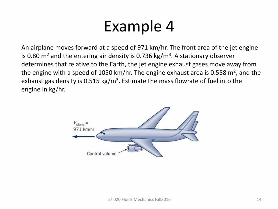
Example 4


An airplane moves forward at a speed of 971 km/hr. The front area of the jet engine is 0.80 m2 and the entering air density is 0.736 kg/m3. A stationary observer determines that relative to the Earth, the jet engine exhaust gases move away from the engine with a speed of 1050 km/hr. The engine exhaust area is 0.558 m2, and the exhaust gas density is 0.515 kg/m3. Estimate the mass flowrate of fuel into the engine in kg/hr.





CS𝛽𝛽𝛽𝛽𝛽𝛽𝑟𝑟 ⋅ 𝑛𝑛𝑑𝑑𝑑𝑑

Assuming 1D flow,−�̇�𝑚fuel − 𝛽𝛽1𝑑𝑑1𝛽𝛽𝑟𝑟1 + 𝛽𝛽2𝑑𝑑2𝛽𝛽𝑟𝑟2 = 0

or�̇�𝑚fuel = 𝛽𝛽2𝑑𝑑2𝛽𝛽𝑟𝑟2 − 𝛽𝛽1𝑑𝑑1𝛽𝛽𝑟𝑟1

Since𝛽𝛽𝑟𝑟1 = 𝛽𝛽1 − 𝛽𝛽plane = 0 − −971 = 971 ⁄km hr

𝛽𝛽𝑟𝑟2 = 𝛽𝛽2 − 𝛽𝛽plane = 1050 − −971 = 2021 ⁄km hrThus,

�̇�𝑚fuel= 0.515 0.558 2021 1000 ⁄m km− 0.515 0.558 2021 1000 ⁄m km = 580,800 − 571,700= 9100 ⁄kg hr

Continuity Equation (Ch. 5.1)


RTT with 𝐵𝐵 = mass and 𝛽𝛽 = 1,

0 =𝐷𝐷𝑚𝑚sys

𝐷𝐷𝐷𝐷mass conservatoin

=𝑑𝑑𝑑𝑑𝐷𝐷�CV𝛽𝛽𝑑𝑑𝛽𝛽 + �

CS𝛽𝛽𝛽𝛽 ⋅ �𝒏𝒏𝑑𝑑𝑑𝑑

or

�CS𝛽𝛽𝛽𝛽 ⋅ �𝒏𝒏𝑑𝑑𝑑𝑑

Net rate of outflowof mass across CS

= −𝑑𝑑𝑑𝑑𝐷𝐷�CV

𝛽𝛽𝑑𝑑𝛽𝛽

Rate of decrease ofmass within CV

Note: Incompressible fluid (𝛽𝛽 = constant)

�𝐶𝐶𝑆𝑆𝛽𝛽 ⋅ �𝒏𝒏𝑑𝑑𝑑𝑑 = −

𝑑𝑑𝑑𝑑𝐷𝐷�𝐶𝐶𝑉𝑉

𝑑𝑑𝛽𝛽 (Conservation of volume)

Simplifications


1. Steady flow

�CS𝛽𝛽𝛽𝛽 ⋅ �𝒏𝒏𝑑𝑑𝑑𝑑 = 0

2. If 𝛽𝛽 = constant over discrete CS’s (i.e., one-dimensional flow)

�CS𝛽𝛽𝛽𝛽 ⋅ �𝒏𝒏𝑑𝑑𝑑𝑑 = �

out

𝛽𝛽𝛽𝛽𝑑𝑑 −�in

𝛽𝛽𝛽𝛽𝑑𝑑

3. Steady one-dimensional flow in a conduit

𝛽𝛽𝛽𝛽𝑑𝑑 out − 𝛽𝛽𝛽𝛽𝑑𝑑 in = 0

or

𝛽𝛽2𝛽𝛽2𝑑𝑑2 − 𝛽𝛽1𝛽𝛽1𝑑𝑑1 = 0

For 𝛽𝛽 = constant

𝛽𝛽1𝑑𝑑1 = 𝛽𝛽2𝑑𝑑2 (or 𝜌𝜌1 = 𝜌𝜌2)

Some useful definitions


• Mass flux (or mass flow rate) �̇�𝑚 = �𝐴𝐴𝛽𝛽𝛽𝛽 ⋅ 𝑑𝑑𝑑𝑑 = 𝛽𝛽𝛽𝛽𝑑𝑑 for uniform flow

• Volume flux (flow rate) 𝜌𝜌 = �𝐴𝐴𝛽𝛽 ⋅ 𝑑𝑑𝑑𝑑 = 𝛽𝛽𝑑𝑑 for uniform flow

• Average velocity �̅�𝑑 =𝜌𝜌𝑑𝑑 =

1𝑑𝑑�𝐴𝐴

𝛽𝛽 ⋅ 𝑑𝑑𝑑𝑑

• Average density �̅�𝛽 =1𝑑𝑑�𝐴𝐴

𝛽𝛽𝑑𝑑𝑑𝑑

Note: �̇�𝑚 ≠ �̅�𝛽𝜌𝜌 unless 𝛽𝛽 = constant

Note: 𝑑𝑑𝑑𝑑 = �𝒏𝒏𝑑𝑑𝑑𝑑

Example 5


Estimate the time required to fill with water a cone-shaped container 5 ft hightand 5 ft across at the top if the filling rate is 20 gal/min.

0 =𝑑𝑑𝑑𝑑𝐷𝐷�CV

𝛽𝛽𝑑𝑑𝛽𝛽 + �CS𝛽𝛽𝛽𝛽 ⋅ �𝒏𝒏𝑑𝑑𝑑𝑑

Apply the RTT for conservation of mass, i.e., 𝛽𝛽 = 1

For incompressible fluid (i.e., 𝛽𝛽 = constant) and one inlet,

0 =𝑑𝑑𝑑𝑑𝐷𝐷�CV

𝑑𝑑𝛽𝛽

=𝑉𝑉(𝑡𝑡)

− 𝛽𝛽𝑑𝑑 in=𝑄𝑄



Volume of the cone at time t,

𝛽𝛽 𝐷𝐷 =𝜋𝜋𝐷𝐷2

12ℎ 𝐷𝐷

Flow rate at the inlet,

𝜌𝜌 = 20galmin

�231in3

gal1,728

in3

ft3= 2.674 ft3/min

The continuity eq. becomes

or𝑑𝑑ℎ𝑑𝑑𝐷𝐷 =

12𝜌𝜌𝜋𝜋𝐷𝐷2 (1)

0 =𝑑𝑑𝑑𝑑𝐷𝐷

𝜋𝜋𝐷𝐷2

12⋅ ℎ − 𝜌𝜌



ℎ 𝐷𝐷 = �0

𝑡𝑡 12𝜌𝜌𝜋𝜋𝐷𝐷2

𝑑𝑑𝐷𝐷 =12𝜌𝜌 ⋅ 𝐷𝐷𝜋𝜋𝐷𝐷2

Solve the 1st order ODE for ℎ(𝐷𝐷),

Thus, the time for ℎ = 5 ft is

𝐷𝐷 =𝜋𝜋𝐷𝐷2ℎ12𝜌𝜌 =

𝜋𝜋 5 ft 2(5 ft)(12)(2.674 ft3/min) = 12.2 min

reynolds transport theorem and continuity equationfluids/posting/lecture_notes/rt… · reynolds...

Documents