revision of the numerical model for the lower hutt groundw… of the numeric… · revision of the...
TRANSCRIPT

Revision of the numerical modelfor the Lower Hutt groundwaterzone
APRIL 2003

APRIL 2003
Revision of the numericalmodel for the Lower Huttgroundwater zone
Prepared for:Greater Wellington – The Regional Council
?phrea tosG R O U N D W A T E R C O N S U L T I N G

Contents1. Introduction...............................................................................................................1
2. Previous modelling .................................................................................................2
3. Data sources.............................................................................................................33.1 Geological data...........................................................................................................33.2 Harbour bathymetry...................................................................................................43.3 Groundwater levels ....................................................................................................43.4 River stage data .........................................................................................................53.5 Groundwater usage...................................................................................................5
4. Hydrogeology...........................................................................................................54.1 The Lower Hutt groundwater zone (LHGZ) ...........................................................54.2 Hydrostratigraphy.......................................................................................................64.2.1 Taita alluvium..............................................................................................................64.2.2 Petone marine beds and melling peat....................................................................74.2.3 Waiwhetu artesian gravels .......................................................................................74.2.4 Wilford shell bed.........................................................................................................94.2.5 Moera gravels .............................................................................................................94.2.6 Deep strata..................................................................................................................94.2.7 Greywacke ................................................................................................................104.3 Hydraulic properties.................................................................................................104.3.1 Taita alluvium............................................................................................................104.3.2 Petone marine beds/melling peat..........................................................................114.3.3 Upper Waiwhetu gravels .........................................................................................114.3.4 Lower Waiwhetu aquifer .........................................................................................124.3.5 Wilford shell beds.....................................................................................................134.3.6 Moera basal gravels ................................................................................................134.3.7 Deep strata................................................................................................................134.3.8 Greywacke ................................................................................................................144.4 Recharge...................................................................................................................144.4.1 River recharge ..........................................................................................................144.4.2 Rainfall recharge ......................................................................................................154.5 Groundwater flows and aquifer discharge ...........................................................16
5. Numerical model design ......................................................................................175.1 Model code................................................................................................................175.2 Finite difference grid design...................................................................................175.3 Model boundaries ....................................................................................................195.4 River simulation........................................................................................................195.4.1 River bed elevation..................................................................................................195.4.2 River stage ................................................................................................................21

5.4.3 River bed conductance ...........................................................................................215.4.4 River spreadsheet....................................................................................................225.4.5 Hutt River south of KGB and Waiwhetu Stream.................................................225.5 Discharge simulation...............................................................................................23
6. Model calibration ...................................................................................................236.1 Procedure..................................................................................................................236.2 Steady state calibration...........................................................................................246.2.1 Input parameters ......................................................................................................256.2.2 Steady state model calibration results..................................................................266.2.3 Steady state calibration verification.......................................................................276.2.4 Steady state model sensitivity analysis................................................................286.3 Transient flow calibration........................................................................................306.3.1 1996-1997 transient calibration.............................................................................306.3.2 14-year calibration...................................................................................................336.3.3 2000-2001 calibration..............................................................................................34
7. Summary and Conclusions ................................................................................35
References.............................................................................................................................37
REVISION OF THE NUMERICAL MODEL FOR THE LOWER HUTT GROUNDWATER ZONE
WELLINGTON REGIONAL COUNCIL, RESOURCE INVESTIGATIONS DEPARTMENT, TECHNICAL REPORT
1
1. IntroductionThe Lower Hutt – Port Nicholson sedimentary basin (Figure 1) contains aregionally important groundwater resource which supplies up to 40% of thewater demand for the greater Wellington region. The basin contains severalconfined artesian, semi-confined and unconfined gravel aquifer units whichcollectively constitute a layered aquifer system known as the Lower HuttGroundwater Zone (LHGZ). Currently, major municipal abstraction takesplace only from the most productive Upper Waiwhetu Artesian Gravels at anaverage rate of approximately 60 ML/day but peaking at 100 ML/day duringthe summer months. Management of the groundwater resource is reliant upona robust evaluation of the sustainable yield in conjunction with a strategicgroundwater level and water quality monitoring system to ensure that salinecoastal waters do not invade the aquifers.
Given increasing abstraction demands on the Lower Hutt Groundwater Zone,there is a need to review the safe yields for groundwater system, and to reviewmanagement safeguards to minimise the risk of saline water intrusion.
Recent advances in the geological and hydrogeological understanding of thegroundwater system prompted the Wellington Regional Council to revise theexisting numerical model (HAM1) built some eight years ago (Reynolds,1993). To avoid inherent limitations of the old model, which focussed onlyupon the Waiwhetu Artesian Gravels and was limited by poor definition of thesystem recharge and discharge mechanisms, construction of an entirely newmodel has been required (HAM2).
The HAM2 has a less complex the spatial zonation of hydraulic properties thanthe previous model, and a more detailed layer structure based upon revisedgeological interpretation of the sedimentary sequence. The model boundarieshave been re-designed allowing aquifer discharge processes to be moreappropriately modelled, and the simulation of recharge through the Hutt Riverbed has been refined. These changes have resulted in an improved calibrationwhich has undergone sensitivity and uncertainty analysis using the automatedparameter estimation routine, PEST (Watermark Computing, 1998).
The objectives of re-building the Hutt Aquifer Model can be summarised asfollows:
• Facilitate the re-assessment and refinement of the sustainable and safeyield of the Waiwhetu Aquifer with greater confidence.
• Enable an assessment of the feasibility and advantages of abstractinggroundwater from lower stratigraphic levels in the Waiwhetu Aquiferthereby increasing the overall safe yield from this aquifer.
• Enable a preliminary safe yield for the Moera Aquifer to be made,together with an effects assessment on the overlying Waiwhetu Aquifer.

REVISION OF THE NUMERICAL MODEL FOR THE LOWER HUTT GROUNDWATER ZONE
WELLINGTON REGIONAL COUNCIL, RESOURCE INVESTIGATIONS DEPARTMENT, TECHNICAL REPORT
2
• Provide an improved understanding of river recharge processes and animproved understanding of the effects of abstraction on groundwaterlevels under various river recharge conditions.
• Contribute towards the process of reviewing the minimum allowableWaiwhetu Aquifer water level at the Petone foreshore.
• Provide a basis for review of the WRC monitoring network.
• This report documents the rebuilding and calibration of the new model -HAM2.
2. Previous modelling
Prior to the current re-build, the most recent version of the Hutt Aquifer Model- HAM1 was based upon an earlier finite difference model developed byReynolds (1993) and later transferred to a more convenient model platform(Visual Modflow) by Pattle Delamore Partners Ltd (1999). This model wasable to simulate a reasonable regional groundwater balance and provide anacceptable transient calibration for the Waiwhetu aquifer. However, it had anumber of inadequacies which had an important bearing on the accuracy of themodel and its predictive capability. These were:
• River – aquifer relationships were not simulated with sufficient accuracyor sensitivity. Bed losses from the Hutt River control the availability ofrecharge to the Waiwhetu and Moera aquifers. The current modelassumed that the river bed conductance was constant regardless of theriver stage, whereas in reality the wetted area for infiltration is highlydependent upon stage.
• The coarse model grid and layer structure inhibited the accurate simulationof local vertical and horizontal flow gradients (ie around wells, rivers anddischarge zones)
• The model was vertically divided somewhat coarsely into an over-simplified layered system, with one layer representing each aquifer unit(i.e. one layer each for the unconfined, Waiwhetu and Moera). It has sincebeen recognised that that the two confined aquifers are internally highlystratified and exhibit vertical variations in hydraulic conductivity andgroundwater head. The current model also assumed fully penetratingwells, whereas all major abstractions occur from only the top portion ofthe Waiwhetu gravels.
• On the basis of recent research, the discharge from the Waiwhetu andMoera aquifers as leakage into Wellington harbour was not appropriatelyrepresented.
• The Moera aquifer was largely ignored and no attempt was made tocalibrate the model for this aquifer.

REVISION OF THE NUMERICAL MODEL FOR THE LOWER HUTT GROUNDWATER ZONE
WELLINGTON REGIONAL COUNCIL, RESOURCE INVESTIGATIONS DEPARTMENT, TECHNICAL REPORT
3
3. Data sources
3.1 Geological data
Re-interpretation of existing and new bore log data, combined with an analysisof the depositional environment of the Lower Hutt valley, have been used torevise the geometry of the LHGZ and characterise the constituenthydrogeological units.
A large number of logs relating to bores drilled over the past century areavailable are stored within a database compiled by the WRC and IGNS. Thedatabase has recently been reviewed and updated (L. Brown, pers comm.).
In the course of the current modeling task, geological logs for bores greaterthan 35m depth were re-examined and interpreted on the basis of the presentunderstanding of the Lower Hutt – Port Nicholson depositional environment.These logs (numbering 30), and the revised interpretations, are contained inAppendix 1. Additional data from some 130 shallower bores stored in thedatabase having depths of between 10m and 35m were used to supplement thedeeper logs and define the three-dimensional nature of the shallower geologicalunits.
Together, additional bore data and the re-interpreted bore logs were used to re-define the geometry of the various hydrogeological units in the LHGZ. Spatialdata defining the top/base boundaries of each unit were then derived byextrapolating the bore data and relying on the anticipated depositionalconfiguration of the sedimentary sequence. Although there is a reasonablespread of bore data throughout the LHGZ, most of the deeper bores are locatedin the Lower Hutt City/Petone area. However, in the upper catchment area,there is sufficient bore data to adequately define the geometry of the shallowunconfined gravels.
The recently drilled Moera Gravel Investigation Bore 6386 (Brown and Jones,2000) was used to supplement the interpretation of the hydrostratigraphy forthe Lower Hutt Groundwater Zone on the basis of detailed geological andgeophysical logging, pump testing and chemical analysis of groundwater andvarious levels in the succession. This bore was drilled to a depth of 151.3m inLower Hutt. Although this bore represents just one geospatial point, theinformation derived from it has aided the re-interpretation other deep boreswhich has in turn aided the revision of the hydrostratigraphic sequence anddepositional characteristics of the LHGZ.
Definition of offshore geology has relied on marine geophysical data (Davyand Wood, 1992; Wood and Davy, 1993; Harding 2000) in conjunction withthe revised depositional model for the basin (L. Brown, pers. comm.). TheSomes Island bores have also been used to locally define the depth andelevation of the base of the Petone Marine Beds. This information has beenused to approximate the offshore geometry and thickness of the varioushydrostratigraphical units used in the model.

REVISION OF THE NUMERICAL MODEL FOR THE LOWER HUTT GROUNDWATER ZONE
WELLINGTON REGIONAL COUNCIL, RESOURCE INVESTIGATIONS DEPARTMENT, TECHNICAL REPORT
4
3.2 Harbour bathymetry
Harbour bathymetry was derived from the 1:200,000 New ZealandOceanographic Institute Chart ‘Cook Straight Bathymetry’ (1996). The datawere used to define the base of the model fixed head cells over the harbour.
3.3 Groundwater levels
The WRC hold a large volume of continuously and intermittently recordedgroundwater level data relating to numerous monitoring sites in the LHGZstored in the Council’s TIDEDA database. The site locations are shown inFigure 2 and details of the bore depths and the available monitoring record arecontained in Table 1.
Table 1: Groundwater level recording sites
Monitoring Bore Depth and aquifer Length ofRecord
McEwan Park
Somes Island
Hutt Recreation Ground
Randwick Reserve
Petone Centennial Museum PCM
Port Road
Bell Park
Hutt Valley Mem Tech Coll HVMTC
Mitchell Park
Taita Intermediate
IBM1
26.2 Upper Waiwhetu
21.2 Upper Waiwhetu (?)
23.5 Upper Waiwhetu
24.4 Upper Waiwhetu
26.2 Upper Waiwhetu
28.7 Upper Waiwhetu
23.2 Upper Waiwhetu
29.6 Upper Waiwhetu
51.8 (?) upper Waiwhetu
14.6 Upper Waiwhetu
114.6 Moera Gravels
1971 – present
1969 – present
1967 – present
1975 – present
1968 – May 1996
1970 – June 1997
1975 – Dec 1995
1968 – June 1996
1968 – present
1968 – present
1992 – present
The monitoring sites listed in Table 1 were used for model calibration. Most ofthe sites are influenced by tidal effects which have been removed frommonitoring data used for steady state model calibration. For transient modelcalibration, 30-day or 10-day mean water levels were used thereby averagingout the tidal effects.
The Somes Island bore has periodically experienced leakage due to damage atthe wellhead. As a consequence, parts of the monitoring record for this bore areunreliable. Periods when the bore was leaking are easily recognisable from thebore hydrograph when noticeably lower pressures were recorded. Large leaksare known to have occurred in the following periods:
1/11/71 – 20/12/711/1/75 – 29/4/931/7/97 – 10/2/98
These periods have been omitted from the model calibration dataset.

REVISION OF THE NUMERICAL MODEL FOR THE LOWER HUTT GROUNDWATER ZONE
WELLINGTON REGIONAL COUNCIL, RESOURCE INVESTIGATIONS DEPARTMENT, TECHNICAL REPORT
5
The Somes Island monitoring site also appears to exhibit random erraticfluctuations in levels which are not associated with leakage of the wellhead.Nearby spring vents through which the artesian aquifers discharge may explainthis phenomenon. Leakage may not occur at a consistent rate from the springsbut rather be characterised by irregular flow and periodic ‘blow-outs’ whichmay be reflected in the aquifer pressures recorded at the nearby Somes Islandmonitoring site. Further discussion on the aquifer discharge mechanisms iscontained in Section 4.5.
3.4 River stage data
Continuous monitoring of river stage at Taita Gorge (site no. 29808) wasacquired from the Council’s TIDEDA database and averaged over the requiredstress period interval for transient flow modelling. The data were then used tocalculate river stage and river width in the model cells between Taita Gorgeand Kennedy Good Bridge (KGB). The methodology is described in Section5.5.
3.5 Groundwater usage
Groundwater usage data from the WRC production wells at the Waterloo andGear Island wellfields, and from industrial bores, was sourced from theCouncil’s WELREC database. At the time of this study, the WELRECdatabase contained data only up to August, 1998. Figure 3 shows the locationsof current major groundwater users in the LHGZ.
4. Hydrogeology
4.1 The Lower Hutt groundwater zone (LHGZ)
A sedimentary basin bounded by low permeability greywacke basement rocksoccupies the Lower Hutt Valley continuing offshore beneath Port Nicholson.The basin contains a sequence of alluvial and marine sediments of severalhundred metres in thickness. Collectively, the numerous gravel aquifersoccurring within this sequence constitute the Lower Hutt Groundwater Zone(LHGZ). The basin structure within greywacke basement is a fault–angledepression formed as a result of downthrow on the eastern side of theWellington Fault zone. The depth to basement, and the folding/faultdislocation of the basement rock, determines the total thickness and attitude ofinfilling sediment. The greatest depth to basement occurs on the western sideof the valley adjacent to the fault which defines the western margin of the basin
Aquifers have been formed by the thick accumulations of alluvial gravelsdeposited by the Hutt River. These are separated by beds of fine grainedmarine sediments which form low permeability confining layers extendingacross much of the basin but petering out north of the Kennedy Good Bridgearea where the aquifers become unconfined. The LHGZ therefore consists of amulti-layered aquifer system containing a series of confined artesian andunconfined aquifers.

REVISION OF THE NUMERICAL MODEL FOR THE LOWER HUTT GROUNDWATER ZONE
WELLINGTON REGIONAL COUNCIL, RESOURCE INVESTIGATIONS DEPARTMENT, TECHNICAL REPORT
6
4.2 Hydrostratigraphy
The principal hydrostratigraphic units within the Lower Hutt – Port Nicholsonsedimentary basin have been formally described by Stevens (1956) and aresummarised in Table 2.
Table 2: Hydrostratigraphic units of the Lower Hutt groundwater zone
Stratigraphic Unit Hydrogeological Unit
Taita Alluvium Unconfined and semi-unconfined aquifers
Melling Peat and Petone Marine Beds Aquitard
Waiwhetu Artesian Gravels – Upper and LowerConfined aquifers separated by interstadialaquitard. Unconfined in north and harbourentrance
Wilford Shell Bed Aquitard
Moera Gravels Confined Aquifer, semi-confined in north
Deeper glacial/interglacial deposits Confined aquifer/aquitard sequence
4.2.1 Taita alluvium
The postglacial Taita Alluvium deposits were defined by Stevens (1956) toinclude all postglacial fluvial deposits filling the Hutt Valley downstream ofTaita Gorge. These deposits form the present day surface of the valley. Thealluvium consists mainly of buried river channel and fan gravel deposits, butthe sequence also includes flood and over bank deposits of sand, silt and clay.The near surface gravels constitute an unconfined aquifer whilst deeper layersin the alluvium exhibit semi-unconfined and confined conditions due to thestratified nature of the deposits.
Inland of the Lower Hutt CBD and north of Kennedy Good Bridge, the TaitaAlluvium is a composite gravel, sand and silt deposit underlying a floodplainsurface conformable with the present day river bed gravels. Groundwater levelsin this area are generally between 3 and 10m depth but are locally influencedby river stage and tidal fluctuations. From Lower Hutt City to the coast, theTaita Alluvium overlies, is interbedded with, and underlies contemporaneouspostglacial Petone Marine Beds and Melling Peat.
Brown and Jones (2000) subdivided the Taita Alluvium into units relevant tothe Hutt Valley hydrogeology which has been carried through to the presentstudy during re-interpretation of bore logs. The depositional relationship of theTaita Alluvium to the Petone Marine Beds and Melling Peat identifies atransgressional (T3), progradational (T2: 6500 - 4000 year BP) andprogradational (T1: 4000 year BP to present day) subdivision of the TaitaAlluvium. This distinction is based on depth, sediment colour and stratigraphicrelationship to units with ages constrained by established geological historyand radiocarbon dating (e.g. Melling Peat and Petone Marine Beds). T3 wasdeposited during the postglacial period of rising sea level from about 14 000 to6500 years BP. The Hutt River was adjusting to the shortening of its courseimposed by the sea transgressing over the land, by entrenching into the lastglaciation floodplain surface, and reworking and spreading the derived material

REVISION OF THE NUMERICAL MODEL FOR THE LOWER HUTT GROUNDWATER ZONE
WELLINGTON REGIONAL COUNCIL, RESOURCE INVESTIGATIONS DEPARTMENT, TECHNICAL REPORT
7
downstream of Taita Gorge and across the Hutt Valley floodplain surface.Down valley from Melling and Waterloo, T3 underlies the Petone Marine Bedsas deposition occurred prior to the rising sea transgressing over the land surfaceand reaching the maximum distance inland 6500 years ago. The progradationalTaita Alluvium deposits (T2) represent former Hutt River courses andfloodplains, associated with the coast being built out into the harbour duringthe relatively stable sea level period of the last 6500 years. The progradationalTaita Alluvium deposits can be divided into two units on the basis of the 4000year BP Melling Peat. The peat and wood layer is interbedded with the TaitaAlluvium. T2 underlies Melling Peat and T1 overlies it in the form of nearsurface gravel channel deposits extending almost to the coast. Both T1 and T2are water bearing and hydraulically connected to the Hutt River, withgroundwater outflows from these units forming springs on the valley floor andin the harbour.
4.2.2 Petone marine beds and melling peat
The Petone Marine Beds form an extensive confining strata or aquitardoverlying the Waiwhetu Gravels and are predominantly fine-grained silt, sandand coarse sand deposits which commonly contain shell and wood fragments.There are also occasional shelly gravel or gravel and sand strata. Thesedeposits accumulated as the sea transgressed over the land during thepostglacial rise in sea level. The coast prograded at its present position oncesea level stabilized around 6500 years BP. The most conspicuous surfaceexpression of the Petone Marine Beds are the beach ridges which occur to thewest of the Hutt River from the Petone foreshore inland as far as Alicetown(Stirling 1992). The Petone Marine Beds are generally 10-20 m thick at thesouthern (or harbour) end of the Hutt Valley, and thin inland forming a wedgeshape deposit. The Petone Marine Beds extend inland as far as Melling Bridgein the west, Waterloo in the centre, and Gracefield in the eastern Lower HuttValley. They are also thicker towards the western side of the valley, probablyas a result of the greater subsidence associated with movement on theWellington Fault. Re-interpretation of seismic reflection surveys carried outby Davy and Wood (1993) by Harding (2000) showed that in the north-easternquadrant of the harbour, the Petone Marine Beds are considerably thinner andinterpreted to be 10-12m thick. Beneath the rest of the inner harbour, themarine beds were estimated to be up to 30m thick.
4.2.3 Waiwhetu artesian gravels
Waiwhetu Artesian Gravels underlie either Petone Marine Beds or TaitaAlluvium and represent the principal aquifer in the LHGZ. Water supply wellsin the Lower Hutt and Petone areas abstract from the uppermost WaiwhetuArtesian Gravels at depths of between 20 and 40 m.
The Waiwhetu Artesian Gravels accumulated in a braided fluviatileenvironment during the last glaciation and extend from Taita Gorge to theharbour entrance area. Onshore, the formation attains a maximum thickness ofabout 55m on the western side of the Hutt Valley, but elsewhere it is typicallybetween 30m and 50m thick. Beneath the harbour, the gravels are thicker inthe north and west, and shallower in the south and east as a result of

REVISION OF THE NUMERICAL MODEL FOR THE LOWER HUTT GROUNDWATER ZONE
WELLINGTON REGIONAL COUNCIL, RESOURCE INVESTIGATIONS DEPARTMENT, TECHNICAL REPORT
8
concentrated deposition in the deeper part of the basin along the WellingtonFault. Geophysical interpretations (Davy and Wood, 1993; Harding, 2000)suggest that the gravels are around 20m thick on the eastern side of theharbour, thickening to as much as 70m alongside the fault in the west.Evidence for prominent palaeochannels from seismic surveys indicates that theriver has historically remained close to the Wellington Fault depositing a largethickness of gravels in this area. However, the river appears to have latershifted to the east of Somes Island as shown by the presence of a majorpalaeochannel towards the top of the gravels. This channel, representing apossible preferential flow path in the aquifer, is overlain by considerablythinner Petone Marine Beds and could be an important conduit for thedischarge of groundwater into the harbour.
The materials comprising this hydrostratigraphical unit are highly variable.Gravel clasts are the predominant lithological component, but there are alsosandy gravel, silty gravel, gravelly sand and sand beds. Sand deposits withinthe Waiwhetu Gravels intersected by some wells are as much as 10m thick.The highly permeable upper gravels are characteristically separated bydiscontinuous lenses of silt, peat and clay of limited lateral extent. However,detailed logging of the recent WRC6386 bore (Brown and Jones 2000) and there-interpretation of other bore logs have identified a laterally persistent aquitardwithin the Waiwhetu Artesian Gravels effectively dividing the unit into twodistinct parts – the Upper Waiwhetu Aquifer and the Lower Waiwhetu Aquifer.
The intra-Waiwhetu aquitard occurs at a depth interval of 46.3 to 54.0m in theWRC6386 bore and consists of sand, silt and clay with interbeddedcarbonaceous material. The unit is recognisable in all other deep borestypically being up to 10m thick and occurring at a depth range of 40 to 70m.The aquitard is probably associated with deposition during a period of warmerclimate (interstadial) coincident with the last interglacial about 30 – 40,000years ago. It appears to have a significant effect on groundwater flow in theaquifer as shown by differing chemical and isotopic signatures of groundwaterabove and below the aquitard (Brown and Jones 2000). Small increases inanions and cations are evident in the Lower Waiwhetu Gravels together with aslight increase in conductivity and pH. Tritium dating of groundwater from theUpper Waiwhetu Gravels indicates an age of < 2.5 years (42.3 m), whilstgroundwater below the aquitard has been dated at 45 years (66.4 m).
The Lower Waiwhetu Artesian Gravels are not rust or black stained like theUpper Waiwhetu Gravels and the matrix is composed of a gritty clay, silt andsand. The down hole neutron log for WRC 6386 shows higher silt and sandcontent compared with the Upper Waiwhetu Gravels. The groundwater levelin the lower gravels is also about 0.5 m higher than above the aquitard.
No deep test bores have been drilled inland of Lower Hutt City. As a resulthere is no direct knowledge of the Waiwhetu Artesian Aquifer characteristicsin this area.

REVISION OF THE NUMERICAL MODEL FOR THE LOWER HUTT GROUNDWATER ZONE
WELLINGTON REGIONAL COUNCIL, RESOURCE INVESTIGATIONS DEPARTMENT, TECHNICAL REPORT
9
4.2.4 Wilford shell bed
The Wilford Shell Bed underlies the Lower Waiwhetu Gravels and comprisespredominantly silt, clay and sand deposits containing shells and minor peatysilts. The unit represents an aquitard separating the Lower Waiwhetu Gravelsfrom the underlying Moera Gravels. The aquitard is regarded to be thickerbeneath Port Nicholson and in the Petone Foreshore area where it attainsapproximately 25m. The depth and thickness of the unit decreases up-valley.
The Wilford Shell Bed was deposited during the high sea levels associated withthe last interglacial period (Kaihihu). In the Hutt Valley, the geographicdistribution of the 12 drillholes penetrating the Wilford Shell Bed is restricted,but the inland extension appears to be at about Knights Road in Lower Hutt.An estuary tidal channel depositional environment is indicated by the shellspresent within these deposits and associated interglacial peat, peaty sand, siltand clay (coastal swamp/estuary palaeo-environment) occur inland as far asMitchell Park. There are thin water bearing sand and gravel layers within theWilford Shell Bed.
4.2.5 Moera gravels
The Moera Gravels are poorly sorted weathered brown gravels associated withriver deposition during the penultimate (Waimea) glaciation and are underlainby a marine aquitard layer and a considerable thickness of older alluvial andmarine deposits. Toward Taita Gorge, the Moera Gravels appear to lie directlyon greywacke basement.
The unit has a thickness of approximately 25m in the Petone/Lower Hutt areaand constitutes a deep artesian aquifer extending beneath Port Nicholson.North of Lower Hutt, the Wilford Shell Beds thin and disappear providing avertical hydraulic continuity between the Moera gravels and the higherWaiwhetu Gravels and Taita Alluvium. Recharge to the deeper aquifers occursin this area.
Only 10 bores (including 4 water supply wells) penetrate Moera Gravels atapproximately 100m depth in the Petone area. However, no wells are presentlyabstracting groundwater from this unit.
Artesian pressures within the Moera Gravels are higher than in the overlyingWaiwhetu aquifers. However, due to the relatively high clay content in theweathered gravels, the hydraulic conductivity is low and recent dating of thegroundwater (Brown and Jones, 2000) has revealed a mean residence time of >60 years and a slightly older residence time at the base of the unit (> 70 years).Groundwater chemistry shows a slight increase in cations and anions comparedwith the overlying Waiwhetu Artesian Aquifer with conductivity increasingslightly with depth.
4.2.6 Deep strata
Beneath the Moera Gravels, a thick succession of ancient alluvial and marinesediments lie on greywacke basement. These sediments thicken southwardsfrom Taita Gorge and occupy the deeper central parts of the Lower Hutt – Port
REVISION OF THE NUMERICAL MODEL FOR THE LOWER HUTT GROUNDWATER ZONE
WELLINGTON REGIONAL COUNCIL, RESOURCE INVESTIGATIONS DEPARTMENT, TECHNICAL REPORT
10
Nicholson Basin. Groundwater chemistry in the deeper gravel zones shows anincrease in total major cations and anions, conductivity, bicarbonate, totalhardness and temperature with depth. This information infers a limited ornegligible groundwater throughflow in the deeper strata.
WRC 6386 was drilled below the base of the Moera Basal Gravels to a totaldepth of 151.3m within a sequence of silty brown-grey gravels and thin silt-rich aquitards units. Prior to the drilling of WRC 6386, only three boreholes(Gear Meat Company - WRC 151; Wellington Meat Export Company wellUWA 2 – WRC 1085; and Parkside Road, Seaview - WRC 1086) had beendrilled and logged to provide lithological information on strata underlying theMoera Gravels. In these bores, Begg and Mazengarb (1996) differentiated asequence of temperate interglacial and cold glacial climate deposits based onpollen assemblages identified by Mildenhall (1995). The glacial/interglacialsequence covers two glacial and three interglacial climate events withdeposition extending back to the Ararata Interglacial (oxygen isotope (OI)climatic stage OI11) of Pillans (1990). In the deepest testbore (WRC 151),stratum immediately overlying greywacke basement can be tentativelycorrelated with oxygen isotope stages back as far as OI13.
4.2.7 Greywacke
The LHGZ is bounded by low-permeability greywacke basement rocks. Thedepth to basement and the folding and fault dislocation of the basement rockhas controlled the total thickness and attitude of infilling sediment. There are48 wells located on the floor of the Lower Hutt Valley that penetrategreywacke. However, only four bores intersect the greywacke basement in thedeeper part of the basin within the confined aquifer zone.
Bore WRC 151 at Petone, just to the east of the Wellington Fault, is located inthe deepest part of the onshore basin and intersects greywacke at 299m.Offshore, the basin is regarded to be considerably deeper adjacent to the faultwith the infilling sediment sequence thinning to the east and to the north.Along the Petone foreshore and in the vicinity of the Somes Island, there isevidence to suggest a complex warping and faulting of the basement.Greywacke outcrops on Somes Island appear to represent part of a fault-bounded horst structure extending to the north beneath the Lower Hutt Valley.Uplift and erosion on the horst may have caused the deeper part of theQuaternary sediment sequence to be truncated.
4.3 Hydraulic properties
4.3.1 Taita alluvium
The Taita Alluvium ranges in thickness from 0 to 16m, thickening towardsTaita Gorge. However, since only one reliable pumping test has beenperformed in the shallow gravels, the hydraulic properties of the TaitaAlluvium are poorly characterised. The pumping test was carried out in ashallow bore at Avalon Studios (R27:732004) and provided a range oftransmissivity values from 2,700 to 52,700 m2 /day, with an average of 4,500

REVISION OF THE NUMERICAL MODEL FOR THE LOWER HUTT GROUNDWATER ZONE
WELLINGTON REGIONAL COUNCIL, RESOURCE INVESTIGATIONS DEPARTMENT, TECHNICAL REPORT
11
m2/day. The test results demonstrate the highly heterogeneous nature of theTaita Alluvium.
4.3.2 Petone marine beds/melling peat
The confined and artesian conditions encountered in Upper Waiwhetu Aquiferdemonstrate that the confining Petone Marine Beds and Melling Peat have alow hydraulic conductivity and are laterally persistent. The beds arepredominantly fine-grained silt, sand and coarse sand deposits commonlycontaining shell and wood fragments or shell beds. Measurements fromvarious construction site investigations provide a horizontal hydraulicconductivity range of 10 to 1x10⁻⁴ m/day (WRC, 1995). Vertical hydraulicconductivity is expected to be several orders of magnitude due to the stratifiednature of the marine beds and the presence of laterally persistent silt layers.
4.3.3 Upper Waiwhetu gravels
The Upper Waiwhetu Gravels above the interstadial aquitard have beenextensively tested during the course of resource investigations over the past 70years or so. The gravels exhibit a wide range of hydraulic properties due tothe rapid fluviatile depositional environment which accumulated laterally andvertically variable sediments. This variability is reflected by the range oftransmissivity values derived from pump testing.
The WRC (1995) have reviewed and re-interpreted existing pump test data forthe Upper Waiwhetu aquifer, the most significant large-scale tests being:
• Wellington Meat Export Company (1933)• Gear Island (1957 and 1967)• Hutt Park (1974)• Gear Island (1991)• Waterloo (1993)
A further pumping test at a rate of 50 ML/day was carried out in the WaterlooWellfield in November 1995 (Butcher, 1996).
Due to difficulties in the interpretation of the early data (Wellington Meat1933, Gear Island, 1957/67 and Hutt Park 1974), only the latest three tests havebeen used up to derive an average transmissivity and storativity for the UpperWaiwhetu Aquifer in the Gear Island and Waterloo Wellfield areas.
Each of the tests resulted in the calculation of a wide range of hydraulicproperty values for each of the monitoring bores. However, given theheterogeneous nature of the aquifer, the calculation of a transmissivity valuefor a particular observation bore may not be representative of the aquifertransmissivity at that point. This is because the analytical theory underlyingthe test interpretation assumes a homogeneous aquifer and radial flowconditions around the pumping bores.
Table 3 presents a summary of hydraulic properties for the Upper WaiwhetuAquifer derived from the three major pumping tests. Geometric mean values

REVISION OF THE NUMERICAL MODEL FOR THE LOWER HUTT GROUNDWATER ZONE
WELLINGTON REGIONAL COUNCIL, RESOURCE INVESTIGATIONS DEPARTMENT, TECHNICAL REPORT
12
for transmissivity and storage coefficient have been calculated for allobservation data and for bores in the immediate vicinity of the wellfield. Thelatter provide an estimate of local hydraulic properties for the aquifer, whilstthe mean of all the observation bores provides an estimate of the averageregional aquifer properties. More emphasis has been placed on the Waterlootests since the earlier Gear Island test was of a short duration (24 hours) andmay as a consequence underestimate the aquifer transmissivity.
Table 3: Average hydraulic properties for the Upper Waiwhetu aquifer derivedfrom pumping tests
Pumping Test
Transmissivitym2/day
(geometricmean)
Storage coefficient(geometric mean)
Gear Island 1991 (24 hours) Bores within 500m of pumping All observation data
Waterloo 1993 (40 hours) Wellfield bores All observation data
Waterloo 1995 (108 hours) Wellfield bores All observation data
23,40022,000
34,90028,000
38,90027,980
1 x 10⁻³
8 x 10⁻⁴
9 x 10⁻⁴
7 x 10⁻⁴
3 x 10⁻⁴
5 x 10⁻⁴
The Waterloo pumping tests suggest that the average aquifer transmissivity forthe Upper Waiwhetu Aquifer is approximately 28,000 m2 /day, locallyincreasing to between 35,000 and 40,000 around the Waterloo Wellfield.
The tests indicate a range in the confined storage coefficient for this aquifer ofbetween 3x10⁻⁴ and 1x10⁻³
.
4.3.4 Lower Waiwhetu aquifer
Since there have been no pumping tests within the Lower Waiwhetu Aquifer,its hydraulic properties are unknown. However, it has been possible to derive aqualitative assessment of the hydraulic conductivity nature of this aquifer usingevidence provided by lithological description and water chemistry. Bothsuggest that the Lower Waiwhetu Aquifer has a significantly lowergroundwater throughflow and correspondingly lower hydraulic conductivity incomparison to the Upper Waiwhetu Aquifer.
The Lower Waiwhetu Aquifer has a higher silt and sand content whencompared with the Upper Waiwhetu gravels suggestive of a lower hydraulicconductivity. In addition, tritium analyses of groundwater from above andbelow the interstadial aquitard provides contrasting ages and flow rates for thetwo aquifers. Groundwater from the Upper Waiwhetu Aquifer is dated at < 2.5years old, whilst groundwater below the interstadial aquitard has a 45 yearmean residence time (Brown and Jones 2000). There is also a small increase in

REVISION OF THE NUMERICAL MODEL FOR THE LOWER HUTT GROUNDWATER ZONE
WELLINGTON REGIONAL COUNCIL, RESOURCE INVESTIGATIONS DEPARTMENT, TECHNICAL REPORT
13
total anions and cations accompanied by a slight increase in conductivity andpH in the Lower Waiwhetu Aquifer.
4.3.5 Wilford shell beds
The Wilford Shell Beds represent an aquitard unit comprising silt, clay andsand deposits. The hydraulic conductivity for this unit is regarded to be similarto the Petone Marine Beds/Melling Peat as it shares comparable lithologicaland depositional characteristics. An average horizontal hydraulic conductivityof between 0.1 and 0.01 m/day has been estimated for the Wilford Shell Bedson the basis of lithology, with the vertical hydraulic conductivity being anorder of magnitude lower due to the occurrence of clay and silt layering.
4.3.6 Moera basal gravels
No reliable hydraulic property data were available to characterise the hydraulicproperties of the Moera Aquifer until Hughes (WRC, 1998) carried out a free-flowing test on bore UWA3 (WRC 320) at a rate of 16 L/sec. Analysis of thetest provided a transmissivity of value of 1,100 – 1,200 m ²/day and a storagecoefficient of 2 x10⁻⁴. More recently, borehole WRC 6386 was screened in theMoera Aquifer between 106.25 and 115.25 m depth and test pumped over aseven-day period at a mean discharge rate of 39.8 L/sec. Unlike the previousflow test, the pumping test was able to stress the aquifer and provide a morerobust determination of the hydraulic properties for the Moera Aquifer.Analysis of the test provided a transmissivity range of 2,100 to 2,600 m²/day,and a storage coefficient in the range of 4 – 8 x 10 -5.
4.3.7 Deep strata
There is minimal information on which to base an assessment of the hydraulicproperties of the deep strata below the Moera Gravels. Short-duration pumpingfor the purpose of water sampling in borehole WRC 6386 from strata below thebase of the Moera Gravels has provided data from which an approximatetransmissivity can be derived. The highest yielding zone below the MoeraGravels attained a discharge rate of 100 L/min (144 m3/day) and a drawdownof 2.8m after 5 hours pumping. Using the Jacob equation, and by assumingtypical confined aquifer variables, the specific capacity for a confined aquifercan be approximated by the following equation (Driscoll,1987):
Q/s = T / 2000where:Q = yield of well, in US gpms = drawdown in well, in feetT = transmissivity, in gpd/ft
Using the recorded specific capacity, an approximate transmissivity for thesilty gravels of 70 m2/day has been derived using the above equation. This issignificantly lower than the overlying Moera Gravels. Since this is the highestyielding zone within the top of the deeper strata encountered in WRC 6386,and since the groundwater chemistry becomes rapidly mineralised withincreasing depth, the deep strata are likely to have a horizontal hydraulicconductivity at least an order of magnitude lower than 70m2/day. The vertical

REVISION OF THE NUMERICAL MODEL FOR THE LOWER HUTT GROUNDWATER ZONE
WELLINGTON REGIONAL COUNCIL, RESOURCE INVESTIGATIONS DEPARTMENT, TECHNICAL REPORT
14
hydraulic conductivity is regarded to be several orders of magnitude lower dueto the silt layering within numerous aquitard zones. Consequently, the deeperstrata have been regarded to be hydraulically isolated from the highergroundwater environment for modelling purposes.
4.3.8 Greywacke
The greywacke basement rocks have an extremely low primary permeabilitywith localised secondary permeability developed along fracture zones and injoint systems. However, many of the larger fracture systems are clay-filled andhence overall the greywacke basement has been assumed to be impermeable.
4.4 Recharge
The Taita Alluvium, Waiwhetu and Moera aquifers receive recharge sourcedfrom leakage through the bed of the Hutt River in the upper part of the LHGZcatchment where the aquifers become unconfined (between Taita Gorge andKennedy Good Bridge). The river has a complex recharge-dischargerelationship with the shallow unconfined Taita Alluvium aquifer, but generallylooses water to underlying aquifers in the area between Taita Gorge andBoulcott/Kennedy Good Bridge. This area is termed the ‘recharge zone’.Between Boulcott and the coastline in the area where the Waiwhetu aquifersare confined, the river is tidal and generally gains groundwater.
A large proportion of the river bed losses in the recharge zone remains in thehighly permeable Taita Alluvium and flows southwards to the coast, or returnsto the river in the lower reaches. Of the total amount of river bed leakage, onlya small percentage reaches the deeper aquifers. The Upper Waiwhetu Aquiferreceives vertically infiltrating water transmitted through the overlying TaitaAlluvium which is in hydraulic continuity with the river bed. Aquifers belowthe Upper Waiwhetu Aquifer exhibit a relatively small throughflow because ofsignificantly lower hydraulic conductivities (reducing with increasing depthand compaction) and lower hydraulic gradients. The recharge dynamics are,however, regarded to be strongly influenced by the abstraction regime.
Direct rainfall infiltration and infiltration of hillslope runoff also contributerecharge to the Taita Alluvium.
4.4.1 River recharge
Quantification of river recharge by the WRC (1995) has relied upon a limitedamount of concurrent flow gaugings, mostly under low flow conditions whenflow measurements are more easily undertaken and when the measurementerrors are small. There are very few concurrent flow gaugings coincident withmean or high flow conditions.
In the LHGZ, the river section between Kennedy Good Bridge and Taita Gorgeis in hydraulic connection with the Taita Alluvium, Waiwhetu Gravels andMoera Gravels due to the absence of continuous impermeable strata.Significant river losses occur in this section of the river where the deeperaquifers are unconfined. Further losses may occur downstream but will not

REVISION OF THE NUMERICAL MODEL FOR THE LOWER HUTT GROUNDWATER ZONE
WELLINGTON REGIONAL COUNCIL, RESOURCE INVESTIGATIONS DEPARTMENT, TECHNICAL REPORT
15
contribute recharge to the Waiwhetu or deeper aquifers due to the interveningconfining Petone Marine Beds.
Historical concurrent flow gaugings have been carried out mostly under verylow flow conditions using WRC river gauging stations at Taita Gorge (29809),Kennedy Good Bridge (29824), and downstream at Boulcott (29811) for theperiod 1939 - 1993. The mean monthly flows at Taita Gorge range fromapproximately 12 to 36 m3/sec whereas all of the concurrent gauging prior to1995 were taken during flows of between 2.3 and 5.7 m3/sec. During the 1995pumping test, Butcher (1996) carried out five concurrent gaugings duringNovember for flows at Taita Gorge of between 11 and 30 m3/sec. The 1995readings provide the only direct quantification of river losses under normalflow conditions to date.
Figure 4 shows the relationship between flow at Taita Gorge and flow atKennedy Good Bridge using all of the Taita Gorge – Kennedy Good Bridgeconcurrent gauging data. The trend line in Figure 4 is highly dependent uponthe 1995 gauging data which lie on the same straight-line trend as the earlierlow-flow data. Regression analysis of the data in Figure 6 provides thefollowing equation which relates flow at Taita Gorge to Flow at Kennedy-Good Bridge:
Kennedy-Good Bridge = 0.974(Taita Gorge) – 912 L/sec
The relationship is similar to that derived by WRC (1995) using the low flowdata only.
Using this relationship and assuming that the straight-line trend can beextrapolated to higher flows, river losses between Taita Gorge and KennedyGood Bridge during average river flow conditions range from approximately100,000 to 160,000 m3/day but do not exceed 80,000 – 85,000 m3 /day underlow flow conditions (for flows of less than 6 m3/sec). The reduction in lossesduring low flows is assumed to be related to the reduced wetted perimeter ofthe river bed (reduced river bed conductance) and the reduced vertical headgradient between the river and underlying aquifer. The broad, flat nature of thechannel profile means that a small change in stage of only half a metre or sowill produce a large change in the wetted channel perimeter and river bedconductance.
4.4.2 Rainfall recharge
Infiltration of rainfall is a secondary source of recharge to the Taita Alluviumand is of minor significance to the deeper Waiwhetu and Moera aquifers.Reynolds (1993) produced a simple soil moisture model to estimate theaverage monthly rainfall recharge. The model is based on the followingassumption:
Recharge = Rainfall - Actual Evapotranspiration - Soil MoistureDeficit

REVISION OF THE NUMERICAL MODEL FOR THE LOWER HUTT GROUNDWATER ZONE
WELLINGTON REGIONAL COUNCIL, RESOURCE INVESTIGATIONS DEPARTMENT, TECHNICAL REPORT
16
Mean monthly recharge values calculated for the Lower Hutt Catchment areshown in Table 4.
Table 4: Estimated rainfall recharge to the Lower Hutt groundwater zone(Reynolds, 1993)
MonthMean
Rechargemm
JanFebMarAprMayJunJul
AugSepOctNovDec
Annual Mean
1883658
11713513810873724145
833
Since much of the Lower Hutt – Petone is built-up, a high proportion of theland area is now impermeable and stormwater is diverted to the sea or the river.As a consequence, the actual recharge will be significantly lower than the soilmoisture balance estimate and it is estimated that only approximately 40% ofthe catchment is open to rainfall recharge.
4.5 Groundwater flows and aquifer discharge
Groundwater flow in the various aquifers occupying the groundwater basinoccurs down-valley to the foreshore, continuing offshore to the southern edgeof the harbour (Figure 5). Throughout the confined zone, hydraulic gradientsare always upwards and discharge from the aquifers occurs through diffusevertical leakage through aquitard layers into overlying aquifers and into thesea. Discharge from the Upper Waiwhetu Aquifer is also known to occur atdiscrete points as submarine springs where the aquitard layer is thin and hasbeen breached. Harding (2000) has identified a number of areas where springdischarges have been identified and measured. The locations of these areas areshown in Figure 6. Many submarine springs occur near basement outcrops,possibly as a result of a seismic decoupling of the unconsolidated sedimentscaused by the different shaking velocities between the basement rocks and thesediments. There are also spring depressions in the harbour floor which arenot associated with the basement contact and which appear to occur in areaswhere the aquitard layer (Petone Marine Beds) is thin or has been breached byhigh artesian pressures and/or liquefaction during seismic activity.
The principal spring discharge zones identified by Harding (op. cit.) are asshown in Figure 6 and are as follows (zone numbers refer to Figure 6):
• off the Hutt River mouth (zone 1)
REVISION OF THE NUMERICAL MODEL FOR THE LOWER HUTT GROUNDWATER ZONE
WELLINGTON REGIONAL COUNCIL, RESOURCE INVESTIGATIONS DEPARTMENT, TECHNICAL REPORT
17
• off Seaview (zone 4)• off the northern tip of Somes island (zone 5)• Falcon Shoals and harbour entrance (zones 7 and 8)
Depressions previously considered to be a major source of artesian leakagefrom the Upper Waiwhetu Aquifer on the south side of Somes Island werefound to exhibit no signs of submarine discharge (Harding, 2000).
The Somes Island monitoring bore lies close to a submarine discharge zone(zone 5, Figure 6) and the monitoring record form this bore may be influencedby the springs. The Somes Island bore periodically experiences largefluctuations in water level and changes in tidal response which could beexplained by accumulations of silt in the spring depressions and intermittent‘blow-outs’ or changes in discharge rate caused by a build-up of artesianpressures, tidal scour or seismic activity.
5. Numerical model design
5.1 Model code
The USGS finite difference numerical model code MODFLOW (McDonaldand Harbaugh, 1988) has been used to re-model the Lower Hutt GroundwaterZone. The ‘Visual Modflow’ graphical interface (Waterloo Hydrogeologic,2000) was used to assist with the processing and analysis of model input andoutput data.
5.2 Finite difference grid design
MODFLOW uses a finite difference solution method which requires the use ofa rectilinear, block-centred spatial grid and one or more layers. The new Huttaquifer model grid covers an area of 19500m x 7200m and is considerablylarger than the previous model domain incorporating much of Port Nicholson,extending southwards to Falcon Shoals at the harbour entrance. To avoidnumerical errors, the grid has been aligned with the principal groundwater flowvector parallel to the valley walls (NE-SW). A variable grid size ranging from1300m at the model boundaries and condensing down to 250m in the areaaround the Hutt River and over the unconfined aquifer area has been employed(Figure 7).
The new model has a different layer structure to the previous Hutt aquifermodel (Reynolds, 1993). Since Visual Modflow does not support an implicitquasi 3-D representation of aquitard units using the MODFLOW VCONTterm, the aquitard units have been explicitly modelled as separate layers. Thisadds an unavoidable increased complexity to the model but has the advantageof enabling the storage effects of the aquitard layers to be incorporated.Consequently, the new model has seven layers based upon thehydrostratigraphical divisions discussed in Section 4.2.
One of the most significant changes in the new model is the splitting of theWaiwhetu Gravels into upper and lower members, the incorporation of the

REVISION OF THE NUMERICAL MODEL FOR THE LOWER HUTT GROUNDWATER ZONE
WELLINGTON REGIONAL COUNCIL, RESOURCE INVESTIGATIONS DEPARTMENT, TECHNICAL REPORT
18
interstadial aquitard, and the simulation of abstraction from only the uppermember. Although the existence of the interstadial aquitard is based onrelatively few deep bores, the inferred depositional environment for this unit(Section 4.2.3) suggests that it is relatively widespread but may be eroded orvery thin in some places. The distinct difference in hydraulic conductivitybetween the upper and lower Waiwhetu gravels, and the absence of abstractionfrom the Lower Waiwhetu Aquifer, means that such uncertainty has minorimplications in terms of the simulation of the Upper Waiwhetu Aquifer. Theaquitard will however exert some control on the system response to abstractionscenarios in the Lower Waiwhetu Aquifer.
Table 5 summarises the model layers and the MODLFOW layer types assignedto each of them. Some of the layers (e.g. layers 2, 4 and 6) represent more thanone hydrostratigraphic unit because the aquitard units represented by theselayers do not extend into the unconfined aquifer area north of Kennedy GoodBridge. In the unconfined area, the layers have been assigned propertiesconsistent with the overlying or underlying aquifer units. Layer Type 3 allowsthe cells in a particular layer to switch between confined or unconfineddepending upon whether the modelled head lies above or below the elevationof the layer top. For instance, in the unconfined area, Layer 2 may becomeunconfined but will remain confined when the overlying Taita Alluvium ispartially saturated. Layers deeper than Layer 2 however maintain confinedaquifer conditions at all times.
Table 5: Model layers
Model Layers MODFLOW Layer Type
Layer 1: Taita Alluvium
Layer 2: Petone Marine Beds – UpperWaiwhetu Gravels
Layer 3: Upper Waiwhetu Gravels
Layer 4: Interstadial deposits – UpperWaiwhetu Gravels
Layer 5: Lower Waiwhetu Gravels
Layer 6: Wilford Shell Beds – MoeraGravels
Layer 7: Moera Gravels
Type 1 – Unconfined
Type 3 – Confined/Unconfined, variable S/T
Type 0 – Confined, constant S/T
Type 0 – Confined, constant S/T
Type 0 – Confined, constant S/T
Type 0 – Confined, constant S/T
Type 0 – Confined, constant S/T
The model layer elevations were derived from bore logs contained in therevised geological database (Section 3.1) and imported into Visual Modflow asx, y, z coordinate files. The spatial data for each layer boundary was thencontoured externally using surfer and carefully edited in areas where noobservation points occur to ensure the generated surfaces maintainedconsistency with the conceptual geological model. This entailed insertingartificial data points to control the contouring process. The Surfer ‘.grd’ fileswere then imported into Visual MODFLOW.

REVISION OF THE NUMERICAL MODEL FOR THE LOWER HUTT GROUNDWATER ZONE
WELLINGTON REGIONAL COUNCIL, RESOURCE INVESTIGATIONS DEPARTMENT, TECHNICAL REPORT
19
5.3 Model boundaries
Maintaining consistency with the conceptual hydrogeological model, thefollowing model boundaries have been assigned:
western boundary coincident with the Wellington Fault
eastern boundary coincident with the junction between the unconsolidatedalluvial and marine sediments and the basementgreywacke which plunges towards the Wellington Fault.
northern boundary at Taita Gorge where the sediments thin and areconstricted within the gorge. Minimal throughflowoccurs at this boundary since the gravels become verythin.
southern boundary the estimated southern extent of the aquifers within thebasin coinciding approximately with the southernboundary of Port Nicholson and the harbour entrancearound Falcon Shoals.
The model boundaries and model domain showing the finite difference grid areshown in Figure 7. No-flow conditions have been assigned to all boundaries.In the unconfined aquifer zone, the base of the model coincides with thegreywacke basement contact, but to the south as the basin deepens rapidly, thebase of the model coincides approximately with the base of the Moera Gravels,which has been assumed to have a relatively constant thickness of 25-30m.
5.4 River simulation
The Hutt River above Kennedy Good Bridge (KGB) is a criticalhydrogeological control since recharge to the aquifers within Lower HuttGroundwater Zone occurs principally via flow losses to groundwater from thissection of river.
Previous models of the groundwater system did not take into account theeffects of significant changes in river bed conductance associated with therelationship between channel width and river stage. The current model hasattempted to incorporate this relationship to simulate temporally variableleakage rates through the bed of the Hutt River north of Kennedy Good Bridge.
5.4.1 River bed elevation
River bed levels and channel profiles measured at approximately 100mintervals down the entire length of the river are available for 1987, 1993 and1998 (Hutt River Gravel Analysis Study, WRC1998). Table 6 shows the riverbed elevations taken from cross sections coinciding with approximately withthe centre point of each river cell (identified by model row number). Therecharging segment of the river is represented by twenty-three 250m2 modelcells.

REVISION OF THE NUMERICAL MODEL FOR THE LOWER HUTT GROUNDWATER ZONE
WELLINGTON REGIONAL COUNCIL, RESOURCE INVESTIGATIONS DEPARTMENT, TECHNICAL REPORT
20
Table 6: River cell data – bed loss reach from Taita Gorge to KGB as used in thetransient flow model
River crosssection umber1200 = Taita
Gorge
ModelRow
Minimumbed elevation
1998m RL
Mean bedlevel
changes(mm)
1987 - 1998
1200
1200
1170
1130
1110
1090
1050
1030
1000
980
950
930
910
880
850
830
810
790
770
760
720
690
640
1
2
3
4
5
6
7
8
9
10
11
12
13
14
15
16
17
18
19
20
21
22
23
23.63
23.63
22.4
22.14
21.2
20.9
18.7
17.3
16.9
16.6
15.5
14.6
13.8
12.6
12.3
10.7
10
8.9
9
9.02
6.6
6.7
6
-603
-603
-466
-205
69
-425
-486
-386
-350
-177
10
-96
-57
-135
87
112
577
247
834
752
234
513
805
Table 6 shows that the bed elevation of the Hutt River between Taita Gorgeand KGB has experienced changes of up to about 0.8m over the past decade.Progradation of the bed has occurred towards KGB in response to reductions ingravel extractions whilst at Taita Gorge the bed has experienced a gradualreduction in level of approximately 0.6m over the same period. This complexshifting of bed levels has not been taken into account in the model for the long-term transient calibration, rather the Taita Gorge monitoring recorded has beencorrected for changes in bed level at Taita Gorge (using the methodologydescribed below). The long-term recession in river stage in response to thereduction in bed level as shown by Figure 8 has important implications on thelong-term transient model calibration (Section 5.4.2).

REVISION OF THE NUMERICAL MODEL FOR THE LOWER HUTT GROUNDWATER ZONE
WELLINGTON REGIONAL COUNCIL, RESOURCE INVESTIGATIONS DEPARTMENT, TECHNICAL REPORT
21
5.4.2 River stage
The development of a relationship between the measured Taita Gorge stageand the stage at each cross-section has been an important requirement of thenew model. The model relies upon the calculation of a river stage at eachcross-section location (Table 6) using the continuous river stage monitoringrecord for Taita Gorge (29809). The WRC have, on the basis of intermittentflow measurements made at various localities down the river, modelled theTaita Gorge stage – cross section stage relationships. These are listed inAppendix 2.
Since the Taita Gorge stage record has shifted in response to the declining bedelevation at this location (Figure 8), the stage monitoring data used for long-term transient calibrations have been normalised to 1998 bed level conditions.During a model calibration run spanning several years, a significant error indownstream river stage calculations will occur if the bed elevation at TaitaGorge be assumed to be constant. This is because river cell stage in the modelis referenced to a datum (mean sea level) and not the river bed. An alternativeand more accurate approach would have been to calculate the change the riverbed levels and the corresponding change in stage for each river cell during thetransient simulation. However, this has not proved possible because therelationships are complex and there are insufficient data for river bed changesto adopt such an approach.
Presently, the relationship between the Taita Gorge stage and downstreamlocations is known for 1998 bed level conditions (Appendix 2). Suchrelationships have not been developed for earlier periods. Therefore, the riverbed elevations in the model have been held constant during transientsimulations (1998 conditions) and the gauging data for Taita Gorge has been‘normalised’ to the 1998 bed level at this site. For instance, if the bed level atTaita Gorge was 0.6m higher than it is now (ie 1987 levels), the measuredTaita Gorge river stage has been reduced by this amount to compensate for thelower bed level set in the model. In this way, the model will allow the correctamount of water into the underlying aquifer using the correct vertical headgradients.
5.4.3 River bed conductance
River bed conductance is a parameter used by MODFLOW which is calculatedusing the length of a reach (L) in each river cell, the width of the river (W) inthe cell, the thickness of a river bed (M), and the hydraulic conductivity of theriver bed material (K). The streambed conductance, C, is expressed as:
C = K L W / M
The river width (W) is dependent upon river stage and can vary enormously inresponse to a relatively small change in river stage resulting in a large changein the river bed conductance. To account for this in the model, the profilescorresponding to each river cell (Table 6) were used to derive a relationshipbetween stage and width (channel wetted perimeter). The relationship isdifferent for each profile due to changes in channel geometry. Therefore eachriver cell between Taita Gorge and KGB has a unique stage – width

REVISION OF THE NUMERICAL MODEL FOR THE LOWER HUTT GROUNDWATER ZONE
WELLINGTON REGIONAL COUNCIL, RESOURCE INVESTIGATIONS DEPARTMENT, TECHNICAL REPORT
22
relationship. The relationships, contained in Appendix 3, are based upon 1998channel profiles derived from the Hutt River Gravel Analysis Study(WRC1998). Comparison of the profiles with those of 1987 and 1993 showsthere to be a relatively small change in channel geometry and therefore therelationships developed for 1998 are considered to be valid for the preceding10 years or so.
5.4.4 River spreadsheet
To calculate the set of unique river bed elevation, river stage and river bedconductance values for each individual river cell between Taita Gorge andKGB for transient flow modelling, a spreadsheet was constructed to performthe following calculations for each model stress period:
• correct the Taita Gorge record for bed level changes if necessary• calculate the river stage for each river cell based on the corrected Taita
Gorge record (Appendix 2)• calculate the channel width based on the river stage in the cell (Appendix
3)• calculate the river bed conductance• format the data for each river cell for importing to Visual Modflow
5.4.5 Hutt River south of KGB and Waiwhetu Stream
To the south of Kennedy Good Bridge (KGB) the Waiwhetu and Moeraaquifers become confined and the river interacts only with the Taita Alluvium.South of Boulcott, flow losses and gains become difficult to evaluate becausethe Hutt River becomes tidal. It is likely that there is a significant return ofgroundwater to the Hutt River from the unconfined aquifer (Reynolds, 1993)but a complex discharge-recharge relationship associated with tidal cycles andstage conditions is anticipated near to the river.
Since there are no groundwater level monitoring sites and river loss/gainmeasurements for the Taita Alluvium south of Boulcott, the model cannot becalibrated in this area. The modelling has focussed on the simulation ofrecharge to the aquifers in the unconfined zone north of KGB, the accuraterepresentation of the confined aquifers and discharge processes. Provided thatgeneral head and gradient conditions in the Taita Alluvium are reasonablyrepresented, errors in river losses will not affect the deeper confined aquifersystem.
In the absence of an adequate understanding of the interaction betweengroundwater and the river in the confined aquifer zone, and the likelycomplexity of the relationship, the river has been simplistically represented inthe model using drain cells south of KGB to the river mouth. MODFLOW'sDrain Package removes water from the aquifer at a rate proportional to thedifference between the head in the aquifer and the elevation of the drain. TheDrain Package assumes that the drain has no effect if the head in the aquiferfalls below the fixed head of the drain and only enables water to be removedfrom the model. The elevation of the drain cells used in the model have beentaken from the 1998 bed levels contained in the Hutt River Gravel Analysis

REVISION OF THE NUMERICAL MODEL FOR THE LOWER HUTT GROUNDWATER ZONE
WELLINGTON REGIONAL COUNCIL, RESOURCE INVESTIGATIONS DEPARTMENT, TECHNICAL REPORT
23
Study (WRC1998) consistent with the bed levels used for the river cells northof KGB. Drain bed conductance values (cf stream bed conductance) wereestimated during calibration.
The Waiwhetu Stream has also been treated as a drain as it is regarded to be aspring-fed stream. Reynolds (1993) also modelled this stream as a drain usingbed levels estimated by the WRC Rivers Department plans and topographicalmaps. The drain levels and bed conductance values used by Reynolds weretransferred to the new model.
5.5 Discharge simulation
Discharge from the confined aquifers takes place through vertical upwardsleakage into the harbour over a broad area, although discharges are also locallymanifest as discrete submarine springs (Section 4.5). The individual springshave not been simulated since their locations and relative dischargecharacteristics are not completely understood. The model handles aquiferdischarge as diffuse leakage principally in areas where the confining beds arethin and where a number of submarine springs have been identified (Harding,2000). Such areas occur in the NE part of the harbour between the Hutt Rivermouth and Somes Island, along the eastern edge of the harbour, and near to theharbour entrance. Unlike the previous model, the new simulation does notcontain any ‘holes’ in the confining beds to facilitate aquifer discharge.
6. Model calibration
6.1 Procedure
The steady state and transient flow calibration process has been carried out infour stages; these are as follows
• initial estimation of parameters and manual (forward) steady-statecalibration
• calibration testing using a second calibration data set• assessment of parameter uncertainty through sensitivity analysis• transient flow calibration (in three stages)
In accordance with standard modelling procedure, the new model was firstsubject to a steady-state calibration process whereby the modelled heads werefitted to a set of assumed steady-state groundwater levels through manipulatingmodel input parameters to achieve a satisfactory match. The calibrationprocess also assessed the predicted water balance for the groundwater systemagainst the model water balance to ensure that the simulation was reasonablyapproximating the conceptual model.
An aquifer is assumed to be in steady-state when the groundwater system is inequilibrium when the stresses and head conditions do not significantly changewith time. In reality, this condition rarely occurs and some stable periodduring which quasi steady-state conditions are observed was chosen for

REVISION OF THE NUMERICAL MODEL FOR THE LOWER HUTT GROUNDWATER ZONE
WELLINGTON REGIONAL COUNCIL, RESOURCE INVESTIGATIONS DEPARTMENT, TECHNICAL REPORT
24
calibration. The calibrated steady state model was then checked by testinganother set of steady-state data.
The following observation data sets were chosen for steady-state calibration:
• 1993 pump test period• 1995 pump test period
The steady-state groundwater flow model was constructed using a reasonabledata set of initial parameters based on the known hydraulic properties of theformations (Section 4.3), and approximate water balance estimates. The inputparameters (hydraulic conductivity, recharge, river bed conductance) were thenadjusted within the constraints of the established range of values until the fitbetween model-generated and observed groundwater heads was minimised anda realistic water balance achieved (by minimising the mean square error). Amanual sensitivity analysis was then carried out on the steady state calibratedmodel to assess the degree of certainty with which the parameters had beenestimated.
Following steady-sate calibration, the model was then run in transient mode fora representative 12 month period (June1996- May1997) and then checkedagainst a 14-year monitoring record for the period 1984 to1998 to confirm thecapability of the model to accurately simulate the long-term behaviour of thesystem under variable stress conditions. The latter simulation was chosen tocommence in 1984 since prior to this there was a major difference in theabstraction regime in the Waiwhetu Artesian Aquifer. The municipal supplywellfield was located at Gear Island (Figure 3) until 1981 and a large numberof industrial abstractions existed in the foreshore area prior to the mid 1980’s.The municipal abstraction wellfield has since moved inland to Waterloo andmost of the large industrial users have gone. Since there are known gaps anderrors in the abstraction database (WELREC) prior to 1984, the long-termcalibration has not included this period.
The transient calibration has partly relied upon the model-independentparameter estimator – PEST (Watermark Computing, 1998) to optimisehydraulic conductivity zone values. PEST is based on the Gauss-Marquardt-Levenberg non-linear least squares algorithm. Hydraulic conductivity valueswere subsequently assessed in terms of sensitivity, uncertainty, covariance andcorrelation from the PEST run. During the PEST run, storage coefficient valueswere held constant and adjusted manually following optimisation of hydraulicconductivity.
A final transient calibration check was subsequently carried out usingmonitoring data collected during the 2000 – 2001 drought period when extremeand prolonged low-flow conditions were experienced in the Hutt River andwhen the aquifer was under severe stress.
6.2 Steady state calibration
Steady state model calibration was initially performed using the groundwaterlevel and abstraction data recorded towards the end of the 1993 pumping test.

REVISION OF THE NUMERICAL MODEL FOR THE LOWER HUTT GROUNDWATER ZONE
WELLINGTON REGIONAL COUNCIL, RESOURCE INVESTIGATIONS DEPARTMENT, TECHNICAL REPORT
25
The data represent assumed quasi steady-state conditions and were used byReynolds (1993) to test the steady state calibration of the earlier model.During this test, the Waterloo Wellfield was abstracting at a constant rate of36,000 m3/day and the Buick Street wells (Figure 3) had a constant output of6,000 m3/day.
The semi-recovered aquifer condition prior to the 1993 test was used byReynolds to calibrate the earlier model before testing the calibration using thedata towards the end of the pumping test. During a recovery period, only theBuick Street wells were pumping. However, it is questionable whether the pre-test groundwater heads represent fully recovered conditions; it is probable thatthey do not. As a consequence, this data has not been used to calibrate the newmodel.
6.2.1 Input parameters
Hydraulic conductivity
Table 7 lists the hydraulic conductivity values used in the steady-state model,based largely upon the established range of values discussed in Section 4.3.Values for vertical hydraulic conductivity (kz) were derived through thecalibration process with each layer having a constant value except for thoselayers containing aquitards. The latter have hydraulic conductivity valuesassigned on the basis of where the aquitard layer is present. Approximatetransmissivity values have been calculated using the average layer thickness.
Table 7: Steady state calibrated hydraulic conductivity values
Confined Zone Unconfined ZoneLayer
#
Hydrostratigraphic
Unit kx,y
m/d
kz
m/d
approx
T m2/d
kx,y
m/d
kz
m/d
approx
T m2/d
1
2
3
4
5
6
7
Taita Alluvium
Petone Marine Beds/Melling Peat
Upper Waiwhetu Gravels
Interstadial Aquitard/UC Gravels
Lower Waiwhetu Gravels
Wilford Shell Beds/UC Gravels
Moeara Gravels
2600
0.1
1120
0.1
600
0.1
80
0.5
0.002
0.1
0.002
0.5
0.002
0.1
20000
28000
10000
2500
2600
1300
1300
1300
600
80
80
0.14
0.14
0.14
0.14
0.5
0.1
0.1
20000
35000
35000
30000
10000
2500
2500
Recharge
River recharge in the unconfined aquifer zone has been based upon the riverstage at Taita Gorge from which the stage in each model cell was calculatedusing the methodology described in Section 5.4.4. The river bed conductancevalue assigned to each cell has assumed a river bed vertical hydraulicconductivity of 10 m/day and a bed thickness of 10m. Table 8 lists the bedconductance values and calculated stage for each model river cell in theunconfined aquifer zone.

REVISION OF THE NUMERICAL MODEL FOR THE LOWER HUTT GROUNDWATER ZONE
WELLINGTON REGIONAL COUNCIL, RESOURCE INVESTIGATIONS DEPARTMENT, TECHNICAL REPORT
26
Table 8: River stage and bed conductance values used in steady state modelcalibration
River Cell(row
number)
CalculatedRiver Stage
River BedConductance
m2/day1234567891011121314151617181920212223
24.0524.0523.2922.5
22.0121.0919.4517.9617.6216.8415.8214.5814.2713.4812.8411.5910.5310.129.539.38.317.476.26
1560015600156001820015600150001620015000175001700013000130001300015600150009000650078001000012000104001690010000
Recharge from rainfall infiltration was conservatively estimated at 300mm/yearfor the entire model domain north of the foreshore, but increased to1000mm/year along the contact between the valley fill alluvium and thegreywacke along the eastern side of the unconfined zone to represent hillsloperunoff recharge. The model is however insensitive to this parameter.
Fixed heads
Layer 1 in the harbour area has a base elevation coincident with the sea floor.The model cells in this area for the top layer were assigned a fixed headcondition of 0m RL to represent the body of water above the Petone MarineBeds which line the harbour floor.
6.2.2 Steady state model calibration results
A number of model runs were performed in order to match the observedgroundwater heads for the initial steady state calibration involving a trial anderror process of adjusting input parameters. Table 9 show the results at the endof this process and Figure 9 is a plot of the same data showing the calibrationstatistics. The root mean square error for the observation data was 0.13m withthe largest residual being 0.29m at the Taita Intermediate observation site.

REVISION OF THE NUMERICAL MODEL FOR THE LOWER HUTT GROUNDWATER ZONE
WELLINGTON REGIONAL COUNCIL, RESOURCE INVESTIGATIONS DEPARTMENT, TECHNICAL REPORT
27
Table 9: Groundwater levels at end November 1993 pumping test used for steadystate model calibration
Monitoring BoreObserved Groundwater
level m RL(corrected for tidal effects)
Modelled Levelm, RL
Residualm
McEwan Park
Somes Island
Hutt Recreation Ground
Randwick Reserve
Petone Centennial Museum
Port Road
Bell Park
Hutt Valley Mem Tech CollMitchell Park
Taita Intermediate
3.82
3.61
4.19
4.15
3.78
3.73
4.15
3.98
5.68
8.7
3.84
3.49
4.32
4.2
3.74
3.81
4.31
4.07
5.62
8.99
0.02
0.12
0.13
0.05
0.04
0.08
0.16
0.09
0.06
0.29
The good initial steady state calibration confirms the integrity of the revisedconceptual groundwater model and the rationalisation of recharge anddischarge processes, together with changes in the model boundaries and layerdefinition.
The water balance for the steady sate calibration is shown in Table 10.
Table 10: Steady state water balance (1993 Waterloo pump test conditions)
Flow Component Inflow m3/day Outflow m3/day
Constant head (Harbour outflow)
Drains (Hutt River + Waiwhetu Stream)
Rainfall recharge
River losses above KGB (Net)
Pumping wells
Balance
28,048
119,271
147,319
28,829
76,490
42,000
147,319
6.2.3 Steady state calibration verification
The steady state calibration was subsequently tested using a second set ofobservation data relating to the November 1995 Waterloo pump test (Butcher,1996). The test had a duration of 4.5 days at a discharge rate of 49.25 ML perday. Quasi-steady state groundwater level conditions were observed towardsthe end of the test. Table 11 and Figure 10 show the water balance and headresiduals respectively for the steady state model verification to 1995 pump testconditions. A reasonable good fit is evident using the same aquifer parametersas the 1993 steady state calibration but using river stage and river bedconductance values based upon the measured Taita Gorge stage during the1995 test.

REVISION OF THE NUMERICAL MODEL FOR THE LOWER HUTT GROUNDWATER ZONE
WELLINGTON REGIONAL COUNCIL, RESOURCE INVESTIGATIONS DEPARTMENT, TECHNICAL REPORT
28
Table 11: Steady state water balance (1995 pump test conditions)
Flow Component Inflow m3/day Outflow m3/day
Constant head (Harbour outflow)
Drains (Hutt River + Waiwhetu Stream)
Rainfall recharge
River losses above KGB (Net)
Pumping wells
Balance
28,785
141,967
170,752
28,476
92,276
50,000
170,752
During the pumping test period, flow losses from the Hutt River were gaugedat between 67,000 and 190,000 with a mean of 130,000 m3/day (Butcher,1996).
Table 12 shows an internal flow analysis for the aquifer system for the 1995calibration using the Zone Budget capability of Visual Modflow to provide anunderstanding of the recharge to each of the aquifer units and the dischargeinto the harbour.
Table 12: Steady state calibration – flow analysis
Flow Component m3/day
Throughflow in Taita Alluvium south of KGB
Total recharge to confined aquifers
Recharge to confined Upper Waiwhetu Aquifer
Recharge to confined Lower Waiwhetu Aquifer
Recharge to confined Moera Gravel Aquifer
Leakage from Upper Waiwhetu Aquifer to harbour
67,830
94,800
77,200
14,500
3,100
30,000
Table 12 shows reasonable agreement with the throughflow (recharge)estimates for the various aquifers made by the WRC (1995, Table 6.16) exceptthat the modelled throughflow for the Upper Waiwhetu is significantly higher(77,200 vs 42,000 m3/day). However, the throughflow in each of the aquifersis influenced by the abstraction regime and the associated change in flowgradients.
6.2.4 Steady state model sensitivity analysis
A manual sensitivity analysis has been carried out on the steady state model toevaluate the degree of uncertainty inherent in the estimation of the principalmodel parameters and stresses during the calibration process. The recognitionof parameter sensitivity has enabled the identification of those parameterswhich have been optimised with a reasonable degree of certainty. Thereliability of the water flux estimations and the predictive capability of themodel hinges on such sensitivity interrogation. Use of the parameterestimation model, PEST, has also been used to assess the correlation and

REVISION OF THE NUMERICAL MODEL FOR THE LOWER HUTT GROUNDWATER ZONE
WELLINGTON REGIONAL COUNCIL, RESOURCE INVESTIGATIONS DEPARTMENT, TECHNICAL REPORT
29
sensitivity of the hydraulic properties assigned to each hydrostratigraphic unitunder transient flow conditions.
Hydraulic conductivity (horizontal and vertical) and river bed leakage north ofKennedy Good Bridge are the dominant parameters to which the model is mostsensitive. These parameters are however strongly correlated and a uniquesolution can be achieved only through observance of the estimated waterbalance for the system and the range of hydraulic conductivity values derivedfrom test pumping investigations.
The model boundaries are defined with a high degree of certainty and thereforea sensitivity analysis for them has not been necessary.
Manual sensitive analysis has consequently been performed on the parameterslisted in Table 13 and graphically reported in Figure 11.
Table 13: Sensitivity analysis parameters
Sensitivity Parameter
rainfall recharge
river bed conductance
kz for the unconfined recharge zone
kx,y for the unconfined zone
kz for the Petone Marine Beds/Melling Peat
kz for the Upper Waiwhetu Confined Aquifer
kx,y for the Upper Waiwhetu Confined Aquifer
kz = vertical hydraulic conductivity; kx,y horizontal hydraulicconductivity in x and y dimensions
The sensitivity analysis involved systematically changing each parameter inturn from the calibrated value by a factor of 0.1, 0.5, 0.75, 1.25, 1.5 and 10.The observed sensitivity of the model to these parameters is shown in Figure11, expressed in terms of the mean of the square root from the sum of thesquared differences between the calculated and observed heads (RMS). Alarge change in the modelled heads resulting from the minor change in aparameter value demonstrates that the model is highly sensitive to thatparameter and the calibrated value is likely to be more accurate dependingupon its correlation to other parameters.
Figure 11 shows that the heads in the Upper Waiwhetu Aquifer are particularlysensitive to the vertical hydraulic conductivity of the Petone Marine Beds,being most sensitive to a decrease in magnitude. This is because this parametereffectively controls the amount of water allowed to flow vertically upwardsand discharge into the harbour from the confined aquifers. Conversely, themodel appears to be relatively insensitive to small changes in the hydraulicconductivity (vertical and horizontal) for the confined Upper WaiwhetuAquifer. Within the unconfined aquifer zone, a higher sensitivity is observedfor both vertical and horizontal hydraulic conductivity because these

REVISION OF THE NUMERICAL MODEL FOR THE LOWER HUTT GROUNDWATER ZONE
WELLINGTON REGIONAL COUNCIL, RESOURCE INVESTIGATIONS DEPARTMENT, TECHNICAL REPORT
30
parameters control the transmittal of water from the river downwards to theunderlying confined aquifers.
The river bed conductance has a relatively small impact on the groundwaterheads in the Upper Waiwhetu Aquifer because the hydraulic properties of theunderlying unconfined gravels control the downwards flow of recharge to theconfined aquifers. Water which is not able to percolate to deeper levelsremains in the Taita Alluvium, or is returned to the river. The river bedconductance value has therefore been estimated on the basis of the amount ofwater released into the model using the concurrent river gauging data as aguideline (Section 4.4).
The model is also insensitive to rainfall recharge which appears to have littlebearing on groundwater head in the Upper Waiwhetu Aquifer. Increasing therainfall recharge by a factor of ten has the effect of raising the RMS by only0.4m. Much of the rainfall recharge in the model is applied to the upper modellayer (Taita Alluvium) over the confined aquifer zone and therefore has noinfluence on the artesian heads unless it is increased greatly over theunconfined zone.
6.3 Transient flow calibration
The objective of undertaking a transient model calibration was to provideverification and confidence that the steady-state model is able to accuratelysimulate the groundwater system under a wide range of boundary andabstraction stress conditions. This has been achieved using a three-step processby first matching the modelled heads to observed heads for a representative 12-month period (1996-97) and undertaking further interrogation of the transientcalibration using the model-independent parameter estimator – PEST(Watermark Computing, 1998) to assess parameter uncertainty and optimisethe hydraulic parameter values. The transient calibration was then testedagainst a 14 year historical monitoring data set (1984 – 98) and against another12-month dataset (2000-2001) to test the model calibration during a severedrought scenario.
6.3.1 1996-1997 transient calibration
The monitoring period June 1996 to May 1997 period was chosen from thelong-term groundwater level record for preliminary transient flow calibrationbeing an apparent ‘average’ year in terms of river stage and groundwater levelconditions. Transient stresses applied to the model were river recharge basedon the stage record for Taita Gorge, abstraction (derived from the WELRECdatabase) and rainfall recharge. River bed conductance as a function ofchannel width (Section 5.4.4), and river stage were the time-dependentvariables controlling river recharge. The river stage at Taita Gorge was notcorrected for bed level variations as these were regarded to be negligible overthe 12-month calibration window.
The 12-month calibration used a 10-day stress period over which abstractionrate, river stage and groundwater levels at observation sites were averaged.Each stress period had ten time steps with a time step multiplier of 1.2.

REVISION OF THE NUMERICAL MODEL FOR THE LOWER HUTT GROUNDWATER ZONE
WELLINGTON REGIONAL COUNCIL, RESOURCE INVESTIGATIONS DEPARTMENT, TECHNICAL REPORT
31
Figure 12 shows the total groundwater abstraction and the observation boredata (dashed lines) for the calibration period.
The process of transient calibration involved assigning storage properties to thehydrostratigraphic units within the established envelope of values derived fromtest pumping. Since the storage properties of the Upper Waiwhetu Aquifer areknown to a reasonable degree of certainty, and the model is relativelyinsensitive to river bed conductance, hydraulic conductivity is the most criticaland sensitive model parameter. Therefore, the transient calibration hasinvolved optimisation and further sensitivity analysis of hydraulic conductivityusing the non-linear automated parameter estimator – PEST (WatermarkComputing, 1998).
PEST was run using the calibrated transient model with the five adjustableparameters listed in Table 14 . The ky values for parameters 1 and 4 were tiedto the kx values. The optimum objective function (or sum of the squaredweighted residuals of groundwater heads) was achieved after 14 optimisationiterations and 163 model calls. The run time for optimisation wasapproximately 8 hours. The optimised parameters and their compositesensitivity is shown in Table 14.
Table 14: Transient model parameter optimisation - hydraulic conductivity
95% confidencelimitsParameter
# ZoneOptimised
valuem/day
Compositesensitivity
lower upper
1
2
3
4
5
kx,y Upper Waiwhetu confined
kz Petone Marine Beds – N foreshore
kz Petone Marine Beds – harbour
kx,y Upper Waiwhetu unconfined
kz Upper Waiwhetu unconfined
1200
0.002
0.002
1350
0.14
0.17
0.085
0.16
0.2
0.2
1047
0.0013
0.0013
1290
0.13
1213
0.0024
0.0017
1462
0.16
The composite sensitivity (unitless) is a measure of the sensitivity of all modeloutputs to a particular parameter. If a parameter has a low compositesensitivity, it will be poorly estimated. Table 14 shows that the verticalhydraulic conductivity (kz) for the Petone Marine Beds north of the foreshore isrelatively insensitive and this parameter has dominated the objective functionduring the estimation process. This means that this parameter may not havebeen estimated well but the 95% confidence interval is small. Comparisonwith the kz for the same unit in the harbour zone shows that both zones can beassigned the same value. The composite sensitivities for the remainingadjustable parameters are relatively high and this is reflected by the small 95%confidence intervals. These parameters will consequently be estimatedreasonably well depending upon the level of correlation with other parameters.
PEST produces a parameter covariance matrix from which a correlationcoefficient matrix is calculated. The correlation coefficient matrix shows thedegree of cross-correlation between elements in the matrix and is shown inTable 15.

REVISION OF THE NUMERICAL MODEL FOR THE LOWER HUTT GROUNDWATER ZONE
WELLINGTON REGIONAL COUNCIL, RESOURCE INVESTIGATIONS DEPARTMENT, TECHNICAL REPORT
32
Table 15: Correlation coefficient matrix
Parameter 1 2 3 4 5
1 1 0.04 0.83 0.04 0.53
2 0.04 1 -0.35 0.3 0.62
3 0.83 -0.35 1 0.05 0.32
4 0.04 0.3 0.05 1 -0.17
5 0.53 0.62 0.32 -0.17 1
The diagonal elements of the correlation coefficient matrix are always unity.The off-diagonal elements always lie between 1 and –1 and the closer the off-diagonal element is to 1 or –1 the more highly correlated are the parameterscorresponding to the row and column numbers (listed in Table 14). Ifparameters are well correlated they can be varied in harmony with little effecton the model calibration and, as a consequence, there will be a high degree ofuncertainty associated with their estimation. Such parameter non-uniquenesscan be overcome by fixing one of the correlated parameters to within a knownrange on the basis of prior information.
The correlation coefficient matrix shows that parameter 3 (kz Petone MarineBeds – harbour zone) shows a high correlation with parameter 1 (kx,y UpperWaiwhetu confined). However, prior information available for the latterparameter was used to restrict its range during the optimisation process andtherefore the optimisation of parameter 3 could be more confidently assigned.A less strong correlation exists between parameters 5 and 1 and parameters 5and 2. Again, since parameter 1 has been restricted using prior information,parameter 5 will have less uncertainty associated with it.
Specific storage and specific yield values used for the calibration lie in themiddle of the range obtained from test pumping investigations and are shownin Table 16 (it should be noted that specific storage = storagecoefficient/aquifer thickness). The plots show a good visual fit between thetwo datasets for all monitoring bores within the Upper Waiwhetu Aquifer andfor the IBM1 bore within the Moera Gravel Aquifer.
Table 16: Calibrated storage properties
Hydrostratigraphic Unit Specific storage, S s Specific yield, S y
Taita Alluvium and Upper Waiwhetu Aquifers
Lower Waiwhetu Aquifer
Moera gravel Aquifer
Aquitard units
7 x 10⁻⁵
1 x 10⁻⁵
1 x 10⁻⁵
1 x 10⁻⁶
0.2
0.15
0.15
0.15
Figure 12 shows the simulated and observed hydrographs for each of theobservation sites using the optimised model. Also shown are the abstraction,river leakage and recharge rates to the Upper Waiwhetu Aquifer. The river

REVISION OF THE NUMERICAL MODEL FOR THE LOWER HUTT GROUNDWATER ZONE
WELLINGTON REGIONAL COUNCIL, RESOURCE INVESTIGATIONS DEPARTMENT, TECHNICAL REPORT
33
leakage rate is highly variable and controlled by river stage and thegroundwater level in the Taita Alluvium. During the 12 month calibrationperiod, net river leakage rates ranged from approximately 100,000 to 170,000m3/day (as 10-day averages) although actual daily rates may have beensignificantly more or less than this average. The flow to the Upper WaiwhetuAquifer remained relatively constant at between 80,000 and 90,000 m3/day andappears to be influenced by abstraction rate, i.e. higher abstraction rates inducemore recharge to the aquifer.
Figures 13 and 14 provide further detailed information to demonstrate that thenew methodology used to simulate the river (Section 5.4) leads to an improvedand reasonable representation of river losses. Figure 13 shows the net riverlosses for representative river cells between Taita Gorge and KGB. The rivercell in model row 2 is located at the northern boundary of the model (TaitaGorge), whilst row 23 is the southernmost river cell at KGB. Significantlygreater losses of between 5,000 and 15,000 m3/day per 250m2 cell occurbetween rows 1 and 5 in the upper 1 – 1.5km reach below Taita Gorge.Between river rows 6 and 20 (3.5km river section), losses per cell are lowerand relatively constant at between 3,000 and 7,000 m3/day per cell. Below row20, the river begins to gain flows back from the aquifer in the confined-unconfined transition zone. The pattern of river losses and river gains shownin Figure 13 is generally consistent with the conceptual hydrogeological model.
Figure 14 shows the flow at Taita Gorge, as input to the model as a river stagebut converted to a flow using the appropriate rating curve, plotted against thesimulated net flow losses (red squares). Also shown are the concurrent gaugingdata (as represented in Figure 4) to check the calibration of the model (bluecircles). The simulated flow losses show a good agreement with the gaugingdata for the 1996-97 transient calibration and also for the extended transient1984-98 calibration (Section 6.3.2).
The model indicates that at flows of greater than approximately 20,000 L/sec(20 cumecs), there is a marked change in the relationship between bed loss andriver flow. Beyond this flow rate, losses tend to reach a plateau at around1,500 – 2,000 L/sec (approx. 130,000 – 170,000 m3/day). However, theaccuracy of this observation cannot be verified in the absence of concurrentgauging data at flow rates of greater than 20,000 L/sec.
6.3.2 14-year calibration
The calibrated transient model was used to simulate historical water leveltrends and recharge fluxes during a 14 year period commencing on 1/1/84. Thesimulation was divided into 30-day stress periods over which system stressesand monitoring data were averaged. Groundwater monitoring data,uncorrected for tidal effects, were also averaged over the stress period. Theuse of 30-day average water levels effectively removes the diurnal tidalfluctuations form the record. Corrections were however performed on theTaita Gorge stage record to compensate for the reduction bed levels over thesimulation period using the methodology described in Section 5.4.2.

REVISION OF THE NUMERICAL MODEL FOR THE LOWER HUTT GROUNDWATER ZONE
WELLINGTON REGIONAL COUNCIL, RESOURCE INVESTIGATIONS DEPARTMENT, TECHNICAL REPORT
34
Figure 15 shows the modelled and observed hydrographs for the calibration. Agood visual fit between the data is apparent for all monitoring in terms of short-and long-term trends in groundwater level. The Somes Island observed recordis unreliable prior to early 1993 (3200 days) due to leakage at the wellhead.After this, the model closely matches the monitoring record for this bore.
The recharge to the Upper Waiwhetu Aquifer is also shown on Figure 15showing a relatively consistent 30-day average recharge rate of 80,000 m3 /day,but increasing to approximately 90-100,000m3/day in response to increasedabstraction rates occurring at about 3700 days (early 1994) . Seasonaldecreases in river leakage rate have a notable effect on groundwater levels asshown by the particularly dry period during the summer of 1994/95 (4100days) which produced a marked depression in groundwater levels which in turninduced greater recharge into the Upper Waiwhetu Aquifer. Within thecalibration window, using 30-day averages, abstraction rates did not exceedrecharge rates to the aquifer. However, this assessment may not hold should asmaller stress period length be considered.
6.3.3 2000-2001 calibration
Following the initial transient calibration procedure, calibration checking wasperformed against the 2000-2001 summer drought period during which riverflows were the lowest on record (1 in 40 year six-monthly low flow rate) andthe aquifer system was under unusual stress.
Figure 16 shows the model calibration for the 2000-2001 year which was rununder 10-day stress periods. Water levels for observation bores and productiondata for the principal abstraction wells (Waterloo Wellfield and Gear Island)were derived from WRC records. Adjustments were made to the river bedconductance value since, under such extreme stress, the river cells were notsupplying sufficient water to the Waiwhetu Gravels. The previous modelcalibration proved to be relatively insensitive to river bed conductance, but itbecame evident during the calibration checking process that the accuracy ofthis parameter is important when vertical hydraulic gradients between the riverbed and the underlying aquifer are accentuated during dry periods.
River bed conductance values were subsequently increased by a factor of 2.4 inorder to achieve a good calibration (Figure 16). No other parameters werealtered. Following re-calibration, the 14 year calibration run was checked. Aslightly better match between observed and modelled data is evident as shownin Figure 17, particularly during low-flow periods when the model previouslytended to over-predict drawdown as a result of insufficient recharge.
The water balance for the calibration, also shown on Figures 16 and 17, showsan increase in river losses which still fall within the range of values obtainedfrom concurrent river gauging data (100 – 200 ML/day). During the 200-2001drought period, recharge to the confined Upper Waiwhetu Aquifer fluctuatedbetween 80 and 100 ML/day, being dependent upon the abstraction rate fromthe Waterloo Wellfield. As extreme low flow conditions in the Hutt Rivercontinued through the summer months, it appeared that water was sourced both

REVISION OF THE NUMERICAL MODEL FOR THE LOWER HUTT GROUNDWATER ZONE
WELLINGTON REGIONAL COUNCIL, RESOURCE INVESTIGATIONS DEPARTMENT, TECHNICAL REPORT
35
from river leakage and from storage release. The latter is shown by a gradualrecession in water level in observation bores (Figure 16).
The re-calibrated model (called HAM Version 2.1) has been adopted forscenario modelling.
7. Summary and Conclusions
The Lower Hutt Groundwater Zone contains a regionally important waterresource which is being exploited from bores located in the Upper WaiwhetuAquifer at a rate approaching the maximum sustainable capacity of the system.
All aquifers are at risk of sea water intrusion should over-abstraction occur,and it is therefore important to quantify the available resource whilstsafeguarding it from the risks of salinisation.
A number of numerical groundwater flow models have been produced for theLower Hutt Groundwater Zone to help assess the characteristics of the systemand predict safe abstraction volumes. Whilst recent models have progressedsome way towards achieving this objective, they possessed limitations in termsof being capable of appropriately simulating recharge and discharge processes.
The conceptual hydrogeological model for the Lower Hutt Groundwater Zonehas been refined during the course of the present study on the basis of re-evaluation of existing geological information, the drilling of a deep explorationbore, and new investigations regarding offshore aquifer discharge mechanisms.
The revised conceptual model has provided the basis for the construction a newHutt Aquifer Model (HAM2). The model has a revised boundary and layerdesign, and an improved method of simulating river recharge. Recharge ratesfrom the river bed to the underlying aquifers have been correlated with riverstage using a temporally variable bed conductivity and calibrated againstmeasured bed losses. Discharge from the confined aquifers has been simulatedto reflect current understanding of sub-harbour aquifer seepage and spring flowcharacteristics.
The principal aquifer unit – the Waiwhetu Artesian Gravels, has been dividedinto two distinct units on the basis evidence from recent drilling, a re-evaluation of pre-existing bore logs, and groundwater chemistry. The UpperWaiwhetu Aquifer contains all current major abstraction bores and isconsiderably more productive than the Lower Waiwhetu Aquifer which liesbeneath an intervening, laterally persistent, aquitard.
The parameter zonation within the HAM2 has been simplified to avoid theunjustified transmissivity zonation adopted in previous models. This hasresulted in an improved steady-state and transient model calibration for theWaiwhetu and Moera aquifers.
Model calibration has been carried out using a combination of manual andautomated methods to optimise input parameters and assess parameter

REVISION OF THE NUMERICAL MODEL FOR THE LOWER HUTT GROUNDWATER ZONE
WELLINGTON REGIONAL COUNCIL, RESOURCE INVESTIGATIONS DEPARTMENT, TECHNICAL REPORT
36
uncertainty and sensitivity. Since critical input parameters and water balancecomponents (storage coefficient, transmissivity, river losses) have beenevaluated through field measurement, there is a reasonable degree ofconfidence associated with the calibration.
Model calibration indicates that the recharge to the Upper Waiwhetu Aquifernormally lies in the range of 80,000 to 100,000 m3 /day. Increased abstractionrates appear to induce more recharge to the aquifer from the river. The short-term maximum recharge rate appears to be approximately 95-100,000 m3/dayunder an abstraction regime of approximately 80,000 m3/day, but is dependentupon concurrent and antecedent river stage conditions.
Further interrogation of the model is required through simulation of variousabstraction and river stage scenarios to provide a comprehensive re-evaluationof the resource.

REVISION OF THE NUMERICAL MODEL FOR THE LOWER HUTT GROUNDWATER ZONE
WELLINGTON REGIONAL COUNCIL, RESOURCE INVESTIGATIONS DEPARTMENT, TECHNICAL REPORT
37
References
Begg, J.G. and Mazengarb, C. 1996. Geology of the Wellington Area. Institute ofGeological and Nuclear Sciences, Geological Map 22.
Brown, L.J. and Jones, A. 2000. Moera Gravel investigation bores WRC well number6386 – Marsden Street, Lower Hutt. WRC/RINV-T-00/30. Wellington RegionalCouncil.
Butcher, G.M. 1996. Report on the pump test carried out on the Waterloo Wellfield,Lower Hutt, November 1995. Prepared for the Hydrological Services Group,Wellington Regional Council.
Davy, B. and Wood, R. 1993. Seismic reflection surveying in Wellington Harbour.prepared for Wellington City Council. Report 553904.
Donaldson, I.G. and Campbell, D.G. 1977. Groundwaters of the Hutt Valley – PortNicholson alluvial basin. DSIR information series No. 124. 78pp.
Driscoll, F.G. 1987. Groundwater and Wells. Johnson Division, Minnesota. 2nd Ed.1089pp.
Harding, S.J. 2000. The characteristics of the Waiwhetu Artesian Aquifer beneathWellington Harbour including the spatial distribution and causes of submarinedischarge. MSc thesis, Victoria University of Wellington.
McDonald, M.G. and Harbaugh, A.W. 1984. A m odular three-dimensional finitedifference groundwater flow model: US Geological Survey Open-File Report 83-875,528pp.
Mildenhall, D.C. 1999. Pleistocene palynology of the Petone and Seaview drillholes,Petone, Lower Hutt valley, North Island, New Zealand. Journal of the Royal Society ofNew Zealand. 25(2): 207-262.
Pillans, 1990. Late Quaternary marine terraces, South Taranaki – Wanganui. NewZealand Geological Survey miscellaneous map 18, 1:100,000. DSIR Wellington.
Reynolds, T.I. 1993. Computer modeling of groundwater and evaluation of scenariosfor pumping from the Waiwhetu Aquifer, Lower Hutt Basin. Volume 1. WellingtonRegional Council, Technical Report WRC/CI-G-93/45
Stevens, G.R. 1956. The stratigraphy of the Hutt Valley, New Zealand. New ZealandJournal of Science and Technology B38: 201-235.
Stirling, M.W. 1992. Late Holocene beach ridges displaced by the Wellington Fault onthe Lower Hutt area, New Zealand. New Zealand Journal of Geology and Geophysics35: 447 – 435.
Tonkin and Taylor, 1992. Water Supply Development Study Phase 1, Volume 4. HuttAquifer modeling. Prepared for Wellington Regional Council.

REVISION OF THE NUMERICAL MODEL FOR THE LOWER HUTT GROUNDWATER ZONE
WELLINGTON REGIONAL COUNCIL, RESOURCE INVESTIGATIONS DEPARTMENT, TECHNICAL REPORT
38
Wood, R. and Davy, B. 1992. Interpretation of geophysical data collected inWellington Harbour. Wellington Regional Council, Report No.1992/78.
WRC, 1995. Hydrology of the Hutt Catchment. Volume 2: Groundwater. WellingtonRegional Council, Hydrological Services Group. Technical Report WRD/CI-T-95/38.
WRC, 1998. Moera aquifer investigation. Wellington Regional Council, ResourcesInvestigation Department. Technical Report WRC/RINV-T-98/13. 34pp
WRC, 1998. Hutt River gravel analysis 1987-1998. Phase Five: OngoingManagement. Hutt River Floodplain Management Plan, Wellington Regional Council.Technical Report WRC/FPSA-T-98/27.

REVISION OF THE NUMERICAL MODEL FOR THE LOWER HUTT GROUNDWATER ZONE
WELLINGTON REGIONAL COUNCIL, RESOURCE INVESTIGATIONS DEPARTMENT, TECHNICAL REPORT
39
Figure 1 : Location map

REVISION OF THE NUMERICAL MODEL FOR THE LOWER HUTT GROUNDWATER ZONE
WELLINGTON REGIONAL COUNCIL, RESOURCE INVESTIGATIONS DEPARTMENT, TECHNICAL REPORT
40
Figure 2 : Groundwater level monitoring sites

REVISION OF THE NUMERICAL MODEL FOR THE LOWER HUTT GROUNDWATER ZONE
WELLINGTON REGIONAL COUNCIL, RESOURCE INVESTIGATIONS DEPARTMENT, TECHNICAL REPORT
41
Figure 3 : Abstraction sites

REVISION OF THE NUMERICAL MODEL FOR THE LOWER HUTT GROUNDWATER ZONE
WELLINGTON REGIONAL COUNCIL, RESOURCE INVESTIGATIONS DEPARTMENT, TECHNICAL REPORT
42
y = 0.974x - 911.59R2 = 0.9915
0
2000
4000
6000
8000
10000
12000
14000
16000
18000
20000
22000
24000
26000
28000
30000
HUTT AT TAITA GORGE (L/s)
Figure 4 : Relationship between flow at Taita Gorge and flow at Kennedy GoodBridge

REVISION OF THE NUMERICAL MODEL FOR THE LOWER HUTT GROUNDWATER ZONE
WELLINGTON REGIONAL COUNCIL, RESOURCE INVESTIGATIONS DEPARTMENT, TECHNICAL REPORT
43
Figure 5 : Groundwater head pattern – upper Waiwhetu aquifer

REVISION OF THE NUMERICAL MODEL FOR THE LOWER HUTT GROUNDWATER ZONE
WELLINGTON REGIONAL COUNCIL, RESOURCE INVESTIGATIONS DEPARTMENT, TECHNICAL REPORT
44
The red regions represent areas that exhibited signs of present day artesianleakage. The green regions represent other areas investigated by Hardingbecause they contained sea floor depressions but were found to have no signsof artesian leakage. The pink triangle show those locations that have beenidentified in the past as having artesian leakage, but were not investigated byHarding because there were no sea floor depressions present on which to baseinvestigations. The blue dots represent areas around Barrett’s Reef whereSCUBA divers have noted disturbance in the water that fits the description ofartesian leakage, but were not investigated because Harding considered theleakage unlikely to be related to the Waiwhetu Artesian Aquifer. The dark reddot represents a suspected submarine spring discharge as detected by NIWAusing side scan sonar during an unrelated study in 1987. Bathymetric contourlines are shown in blue at 5m intervals.
Figure 6 : Location map of identified submarine spring discharge zonesin Wellington Harbour (from Harding, 2000).

REVISION OF THE NUMERICAL MODEL FOR THE LOWER HUTT GROUNDWATER ZONE
WELLINGTON REGIONAL COUNCIL, RESOURCE INVESTIGATIONS DEPARTMENT, TECHNICAL REPORT
45
Figure 7 : Model grid
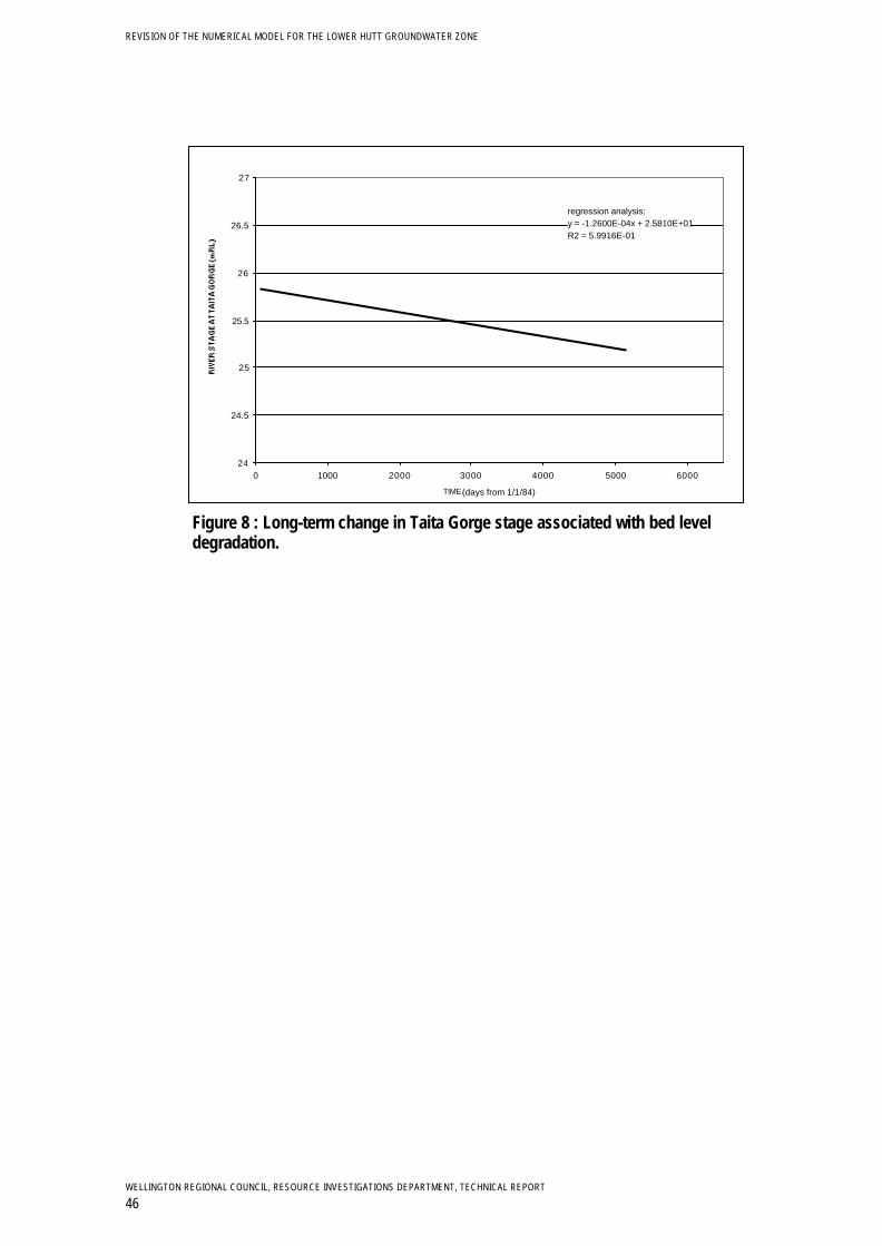
REVISION OF THE NUMERICAL MODEL FOR THE LOWER HUTT GROUNDWATER ZONE
WELLINGTON REGIONAL COUNCIL, RESOURCE INVESTIGATIONS DEPARTMENT, TECHNICAL REPORT
46
regression analysis:y = -1.2600E-04x + 2.5810E+01R2 = 5.9916E-01
24
24.5
25
25.5
26
26.5
27
0 1000 2000 3000 4000 5000 6000
TIME (days from 1/1/84)
Figure 8 : Long-term change in Taita Gorge stage associated with bed leveldegradation.

REVISION OF THE NUMERICAL MODEL FOR THE LOWER HUTT GROUNDWATER ZONE
WELLINGTON REGIONAL COUNCIL, RESOURCE INVESTIGATIONS DEPARTMENT, TECHNICAL REPORT
47
Num.Points : 10
Mean Error : 0.05951333 (meters)
Mean Absolute : 0.1045442 (meters)
Standard Error of the Estimate : 0.03797196 (meters)
Root mean squared : 0.1285249 (meters)
Normalized RMS : 2.525048 ( % )
2
3
4
5
6
7
8
9
10
11
12
2 3 4 5 6 7 8 9 10 11 12
OBSERVED HEAD (m)
Figure 9 : Steady state calibration: 1993 Waterloo pumping test

REVISION OF THE NUMERICAL MODEL FOR THE LOWER HUTT GROUNDWATER ZONE
WELLINGTON REGIONAL COUNCIL, RESOURCE INVESTIGATIONS DEPARTMENT, TECHNICAL REPORT
48
Num.Points : 10Mean Error : 0.2958776 (meters)Mean Absolute : 0.3077586 (meters)Standard Error of the Estimate : 0.05292115 (meters)Root mean squared : 0.3357817 (meters)Normalized RMS : 5.263037 ( % )
2
3
4
5
6
7
8
9
10
11
12
2 3 4 5 6 7 8 9 10 11 12
OBSERVED HEAD (m)
Figure 10: Steady state calibration: 1995 Waterloo pumping test

REVISIO
N O
F THE N
UM
ERIC
AL MO
DEL FO
R TH
E LOW
ER H
UTT G
RO
UN
DW
ATER ZO
NE
WELLIN
GTO
N R
EGIO
NAL C
OU
NC
IL RESO
UR
CE IN
VESTIGATIO
NS D
EPARTM
ENT TEC
HN
ICAL R
EPOR
T
49
Rainfall Recharge
0
0.1
0.2
0.3
0.4
0.5
10 1.5 1.25 1 0.75 0.5 0.1
Parameter adjustment factor
Cha
nge
in R
MS
(m
)
River Bed Conductance
0
0.1
0.2
0.3
0.4
0.5
10 1.5 1.25 1 0.75 0.5 0.1
Parameter adjustment factor
Cha
nge
in R
MS
(m
)
5.3
K (vertical) Unconfined Zone
-0.1
0
0.1
0.2
0.3
0.4
0.5
0.6
10 1.5 1.25 1 0.75 0.5 0.1
Parameter adjustment factor
Cha
nge
in R
MS
(m
)
K (horizontal) Unconfined Zone
-0.5
0
0.5
1
1.5
2
2.5
3
10 1.5 1.25 1 0.75 0.5 0.1
Parameter adjustment factorC
hang
e in
RM
S (
m)
3.4

WELLIN
GTO
N R
EGIO
NAL C
OU
NC
IL RESO
UR
CE IN
VESTIGATIO
NS D
EPARTM
ENT TEC
HN
ICAL R
EPOR
T
50
REVISIO
N O
F THE N
UM
ERIC
AL MO
DEL FO
R TH
E LOW
ER H
UTT G
RO
UN
DW
ATER ZO
NE
K (horizontal) Upper Waiwhetu Confined Zone
-0.5
0
0.5
1
1.5
2
2.5
10 1.5 1.25 1 0.75 0.5 0.1
Parameter adjustment factor
Cha
nge
in R
MS
(m
)
K (vertical) Upper Waiwhetu Confined Zone
0
0.1
0.2
0.3
0.4
0.5
10 1.5 1.25 1 0.75 0.5 0.1
Parameter adjustment factor
Cha
nge
in R
MS
(m
)
K (vertical) Petone Marine Beds
-0.5
0
0.5
1
1.5
2
2.5
10 1.5 1.25 1 0.75 0.5 0.1
Parameter adjustment factor
Cha
nge
in R
MS
(m)
Figure 11 : Steady state model sensitivity analysis

REVISION OF THE NUMERICAL MODEL FOR THE LOWER HUTT GROUNDWATER ZONE
WELLINGTON REGIONAL COUNCIL, RESOURCE INVESTIGATIONS DEPARTMENT, TECHNICAL REPORT
51
1
2
3
4
5
6
7
8
9
10
11
0 50 100 150 200 250 300 350 400TIME (days from 1/6/96)
Mitchell Pk mod
Mitchell Pk obs
McEwan Pk mod
McEwan Pk obs
Taita Int mod
Taita Int obs
IBM1 mod
IBM1 obs
0
20000
40000
60000
80000
100000
120000
140000
160000
180000
0 50 100 150 200 250 300 350 400TIME (days from 1/6/96)
River leakage
Abstraction
Flow to UpperWaiwhetu Aquifer
m3/day
0
1
2
3
4
5
6
7
8
0 50 100 150 200 250 300 350 400TIME (days from 1/6/96)
Somes mod
Somes obs
Hutt Rec mod
Hutt Rec obs
Figure 12 : Transient calibration June 1996 – June 1997 (10-day stress periods)

REVISION OF THE NUMERICAL MODEL FOR THE LOWER HUTT GROUNDWATER ZONE
WELLINGTON REGIONAL COUNCIL, RESOURCE INVESTIGATIONS DEPARTMENT, TECHNICAL REPORT
52
-5000
-3000
-1000
1000
3000
5000
7000
9000
11000
13000
15000
0 50 100 150 200 250 300 350 400
DAYS FROM 1/6/96
Row 2
Row 8
Row 13
Row 19
Row 23
Figure 13 : Simulated river bed losses at selected model rows.

REVISION OF THE NUMERICAL MODEL FOR THE LOWER HUTT GROUNDWATER ZONE
WELLINGTON REGIONAL COUNCIL, RESOURCE INVESTIGATIONS DEPARTMENT, TECHNICAL REPORT
53
Figure 14 : Model calibration – simulated river bed losses vs flow at Taita Gorge
0
500
1000
1500
2000
2500
3000
3500
4000
0 10000 20000 30000 40000 50000 60000 70000 80000
FLOW RATE - HUTT AT TAITA GORGE (L/sec)
simulated loss
observed loss
1996-97 Calibration
0
500
1000
1500
2000
2500
3000
3500
4000
0 10000 20000 30000 40000 50000 60000 70000 80000 90000
FLOW RATE - HUTT AT TAITA GORGE (L/sec)
observed loss
Simulated loss
1984-98 Calibration

REVISION OF THE NUMERICAL MODEL FOR THE LOWER HUTT GROUNDWATER ZONE
WELLINGTON REGIONAL COUNCIL, RESOURCE INVESTIGATIONS DEPARTMENT, TECHNICAL REPORT
54
Figure 15 : Transient model calibration – 14 year period (1984-1998).
0
1
2
3
4
5
6
7
8
9
10
0 500 1000 1500 2000 2500 3000 3500 4000 4500 5000 5500
Taita Int Mod
Taita Int Obs
Mitchell Pk Mod
Mitchell Pk Obs
McEwan Pk Mod
McEwan Pk Obs
DAYS (from 1/1/84)
0
20000
40000
60000
80000
100000
120000
140000
160000
180000
0 500 1000 1500 2000 2500 3000 3500 4000 4500 5000 5500
River loss
Abstraction
Recharge toUpper Waiwhetu
m3/day
DAYS (from 1/1/84)
0
1
2
3
4
5
6
7
8
9
10
0 500 1000 1500 2000 2500 3000 3500 4000 4500 5000 5500
Somes Mod
Somes Obs
Randwick Mod
Randwick obs
DAYS (from 1/1/84)

REVISION OF THE NUMERICAL MODEL FOR THE LOWER HUTT GROUNDWATER ZONE
WELLINGTON REGIONAL COUNCIL, RESOURCE INVESTIGATIONS DEPARTMENT, TECHNICAL REPORT
55
Figure 16 : Transient calibration verification
0
1
2
3
4
5
6
7
8
9
10
11
0 50 100 150 200 250 300 350 400
DAYS (from 1/6/00)
Taita Mod
Mitch Mod
McEwan Mod
Taita Obs
Mitch Obs
McEwan Obs
0
50000
100000
150000
200000
250000
0 50 100 150 200 250 300 350 400
DAYS (from 1/6/00)
24.6
24.8
25
25.2
25.4
25.6
25.8
26
Net River Leakage
Abstraction
Recharge to UWA
River stage

REVISION OF THE NUMERICAL MODEL FOR THE LOWER HUTT GROUNDWATER ZONE
WELLINGTON REGIONAL COUNCIL, RESOURCE INVESTIGATIONS DEPARTMENT, TECHNICAL REPORT
56
Figure 17 : HAM2 2000-2001 recalibration: 14 year run (1983-1998)

WELLIN
GTO
N R
EGIO
NAL C
OU
NC
IL RESO
UR
CE IN
VESTIGATIO
NS D
EPARTM
ENT TEC
HN
ICAL R
EPOR
T
57
REVISIO
N O
F THE N
UM
ERIC
AL MO
DEL FO
R TH
E LOW
ER H
UTT G
RO
UN
DW
ATER ZO
NE
Appendix One – Reinterpretation of deep bore logs
Coding of stratigraphic and aquifer units –
Fill fRecent fluvial rTaita 1 1Taita 2 2Taita 3 3Taita undifferentiated tMelling peat mPetone pWaiwhetu hInterstadial aDeep Waiwhetu wWilford lMoera oOI 7 7OI 8 8OI 9 9OI 10 10OI 11 11OI 12 12OI 13 13Greywacke gColluvium c

WELLIN
GTO
N R
EGIO
NAL C
OU
NC
IL RESO
UR
CE IN
VESTIGATIO
NS D
EPARTM
ENT TEC
HN
ICAL R
EPOR
T
58 REVISIO
N O
F THE N
UM
ERIC
AL MO
DEL FO
R TH
E LOW
ER H
UTT G
RO
UN
DW
ATER ZO
NE
Wells used to revise the Hutt Aquifer model:
Sequence No. Easting Northing Collar RL Depth from Depth to RL Depthfrom
RL Depth to Unit
124 2667060 5996350 2.1 0 0.7 2.1 1.4 f0.7 27.7 1.4 -25.6 p27.7 30.8 -25.6 -28.7 330.8 45.1 -28.7 -43 h
Sequence No. Easting Northing Collar RL Depth from Depth to RL Depthfrom
RL Depth to Unit
141 2670124 5994942 1.5 0 0.5 1.5 1 r0.5 1.5 1 0 p1.5 10.1 0 -8.6 110.1 15.2 -8.6 -13.7 p15.2 18.3 -13.7 -16.8 318.3 30.2 -16.8 -28.7 h30.2 32.2 -28.7 -30.7 a32.2 41.5 -30.7 -40 w41.5 47.2 -40 -45.7 l
Sequence No. Easting Northing Collar RL Depth from Depth to RL Depthfrom
RL Depth to Unit
142 2668820 5996640 1.5 0 4.6 1.5 -3.1 14.6 12.8 -3.1 -11.3 212.8 20.1 -11.3 -18.6 p20.1 21.6 -18.6 -20.1 321.6 43.6 -20.1 -42.1 h43.6 47.6 -42.1 -46.1 a47.6 66.5 -43.1 -65 w66.5 83.8 -65 -82.3 l83.8 114.6 -82.3 -113.1 o114.6 128 -113.1 -126.5 7

WELLIN
GTO
N R
EGIO
NAL C
OU
NC
IL RESO
UR
CE IN
VESTIGATIO
NS D
EPARTM
ENT TEC
HN
ICAL R
EPOR
T
59
REVISIO
N O
F THE N
UM
ERIC
AL MO
DEL FO
R TH
E LOW
ER H
UTT G
RO
UN
DW
ATER ZO
NE
Sequence No. Easting Northing Collar RL Depth from Depth to RL Depthfrom
RL Depth to Unit
151 2666910 5996110 2.4 0 0.9 2.4 1.5 f0.9 4 1.5 -1.6 l4 28 -1.6 -25.6 p28 32.3 -25.6 -29.9 332.3 52.1 -29.9 -49.7 h52.1 53.9 -49.7 -51.5 a53.9 82.8 -51.5 -80.4 w82.8 106.1 -80.4 -103.7 l106.1 135.2 -103.7 -132.8 o135.2 143.9 -132.8 -141.5 7143.9 151.3 -141.5 -148.9 8151.3 183.8 -148.9 -181.4 9183.8 204.5 -181.4 -202.1 10204.5 216.7 -202.1 -214.3 11216.7 239.3 -214.3 -236.9 12239.3 299 -236.9 -296.6 13299 311.2 -296.6 -308.8 g
Sequence No. Easting Northing Collar RL Depth from Depth to RL Depthfrom
RL Depth to Unit
319 2666880 5996170 2.7 0 2.7 2.7 0 p2.7 4 0 -1.3 l4 23.8 -1.3 -21.1 p23.8 30.5 -21.1 -27.8 330.5 49.4 -27.8 -46.7 h49.4 52.9 -46.7 -50.2 a52.9 84.1 -50.2 -81.7 w84.1 104.9 -81.7 -102.2 l104.9 114.6 -102.2 -111.9 o

WELLIN
GTO
N R
EGIO
NAL C
OU
NC
IL RESO
UR
CE IN
VESTIGATIO
NS D
EPARTM
ENT TEC
HN
ICAL R
EPOR
T
60 REVISIO
N O
F THE N
UM
ERIC
AL MO
DEL FO
R TH
E LOW
ER H
UTT G
RO
UN
DW
ATER ZO
NE
Sequence No. Easting Northing Collar RL Depth from Depth to RL Depthfrom
RL Depth to Unit
320 2666820 5996220 2.6 0 0.9 2.6 1.7 f0.9 25.6 1.7 -23 p25.6 28.7 -23 -26.1 328.7 53.7 -26.1 -51.1 h53.7 61.9 -51.1 -59.3 a61.9 82.9 -59.3 -80.3 w82.9 103.9 -80.3 -101.3 l103.9 114.6 -101.3 112 o
Sequence No. Easting Northing Collar RL Depth from Depth to RL Depthfrom
RL Depth to Unit
1085 2668350 5997000 1.4 0 0.3 1.4 1.1 f0.3 5.2 1.1 -3.8 l5.2 22.9 -3.8 -21.5 p22.9 23.5 -21.5 -22.1 323.5 50.6 -22.1 -49.2 h50.6 53.3 -49.2 -51.9 a53.3 73.2 -51.9 -71.8 w73.2 90.5 -71.8 -89.1 l90.5 116.7 -89.1 -115.3 o116.7 124.1 -115.3 -122.7 7124.1 134.1 -122.7 -132.7 8
Sequence No. Easting Northing Collar RL Depth from Depth to RL Depthfrom
RL Depth to Unit
1086 2669835 5994960 1.8 0 1.8 1.8 0 f1.8 5.8 0 -4 l5.8 21 -4 -19.2 p21 23.3 -19.2 -21.5 323.3 41.8 -21.5 -40 h41.8 42.4 -40 -40.6 a42.4 48.8 -40.6 -47 w

WELLIN
GTO
N R
EGIO
NAL C
OU
NC
IL RESO
UR
CE IN
VESTIGATIO
NS D
EPARTM
ENT TEC
HN
ICAL R
EPOR
T
61
REVISIO
N O
F THE N
UM
ERIC
AL MO
DEL FO
R TH
E LOW
ER H
UTT G
RO
UN
DW
ATER ZO
NE
48.8 65.2 -47 -63.4 l65.2 73.2 -63.4 -71.4 o73.2 83.5 -71.4 -81.7 783.5 123.7 -81.7 -121.9 8123.7 130.1 -121.9 -128.3 9130.1 151.9 -128.3 -150.1 10151.9 156.4 -150.1 -154.6 11156.4 175.3 -154.6 -173.5 12175.3 181.4 -173.5 -179.6 g
Sequence No. Easting Northing Collar RL Depth from Depth to RL Depthfrom
RL Depth to Unit
1116 2671620 5998530 9 0 1.4 9 7.6 r1.4 3 7.6 6 l3 7 6 2 27 15.2 2 -6.2 315.2 38.7 -6.2 -29.7 h38.7 45.4 -29.7 -36.4 a45.4 51.8 -36.4 -42.8 w
Sequence No. Easting Northing Collar RL Depth from Depth to RL Depthfrom
RL Depth to Unit
1129 2669950 5994840 1.8 0 0.9 1.8 0.9 f0.9 1.8 0.9 0 r1.8 5.2 0 -3.4 l5.2 18.5 -3.4 -16.7 p18.5 19.2 -16.7 -17.4 319.2 45.1 -17.4 -43.3 a45.1 45.7 -43.3 -43.9 h

WELLIN
GTO
N R
EGIO
NAL C
OU
NC
IL RESO
UR
CE IN
VESTIGATIO
NS D
EPARTM
ENT TEC
HN
ICAL R
EPOR
T
62 REVISIO
N O
F THE N
UM
ERIC
AL MO
DEL FO
R TH
E LOW
ER H
UTT G
RO
UN
DW
ATER ZO
NE
Sequence No. Easting Northing Collar RL Depth from Depth to RL Depthfrom
RL Depth to Unit
1139 2670425 5994650 2.6 0 1.8 2.6 0.8 f1.8 18.7 0.8 -16.1 p18.7 21.3 -16.1 -18.7 321.3 38.4 -18.7 -35.8 h38.4 40.2 -35.8 -37.6 a
Sequence No. Easting Northing Collar RL Depth from Depth to RL Depthfrom
RL Depth to Unit
1149 2670040 5995500 1.9 0 1.8 1.9 0.1 p1.8 4.6 0.1 -2.7 l4.6 6.1 -2.7 -4.2 m6.1 14.9 -4.2 -13 p14.9 18.3 -13 -16.4 318.3 41.2 -16.4 -39.3 h41.2 44.4 -39.3 -42.5 a44.4 48.8 -42.5 -46.9 w48.8 61.6 -46.9 -59.7 l61.6 73.6 -59.7 -71.7 o
Sequence No. Easting Northing Collar RL Depth from Depth to RL Depthfrom
RL Depth to Unit
1176 2671010 5997510 6.3 0 0.6 6.3 5.7 f0.6 2 5.7 4.3 r2 7 4.3 -0.7 27 7.2 -0.7 -0.9 p7.2 30 -0.9 -23.7 330 43.2 -23.7 -36.9 h43.2 48.7 -36.9 -42.3 a48.7 61 -42.3 -54.7 w61 65.2 -54.7 -58.9 l

WELLIN
GTO
N R
EGIO
NAL C
OU
NC
IL RESO
UR
CE IN
VESTIGATIO
NS D
EPARTM
ENT TEC
HN
ICAL R
EPOR
T
63
REVISIO
N O
F THE N
UM
ERIC
AL MO
DEL FO
R TH
E LOW
ER H
UTT G
RO
UN
DW
ATER ZO
NE
Sequence No. Easting Northing Collar RL Depth from Depth to RL Depthfrom
RL Depth to Unit
1177 2669960 5997750 4.5 0 1 4.5 3.5 f1 4.9 3.5 -0.4 l4.9 7.9 -0.4 -3.4 m7.9 9.8 -3.4 -5.3 29.8 11 -5.3 -6.5 p11 17.5 -6.5 -13 317.5 42 -13 -37.5 h
Sequence No. Easting Northing Collar RL Depth from Depth to RL Depthfrom
RL Depth to Unit
1223 2666435 5996255 2.3 0 0.8 2.3 1.5 f0.8 12.2 1.5 -9.9 p12.2 25.8 -9.9 -23.5 325.8 48.9 -23.5 -46.6 h
Sequence No. Easting Northing Collar RL Depth from Depth to RL Depthfrom
RL Depth to Unit
1224 2666375 5996235 0.5 0 9.4 0.5 -8.9 p9.4 14.9 -8.9 -14.4 314.9 40 -14.4 -39.5 h40 43 -39.5 -42.5 a43 79.3 -42.5 -78.8 w79.3 107.6 -78.8 -107.1 l107.6 112.4 -107.1 -111.9 o112.4 117 -111.9 -116.5 7117 118.4 -116.5 -117.9 g

WELLIN
GTO
N R
EGIO
NAL C
OU
NC
IL RESO
UR
CE IN
VESTIGATIO
NS D
EPARTM
ENT TEC
HN
ICAL R
EPOR
T
64 REVISIO
N O
F THE N
UM
ERIC
AL MO
DEL FO
R TH
E LOW
ER H
UTT G
RO
UN
DW
ATER ZO
NE
Sequence No. Easting Northing Collar RL Depth from Depth to RL Depthfrom
RL Depth to Unit
1238 2667750 5996330 3.5 0 1.2 3.5 2.3 f1.2 5.7 2.3 -2.2 l5.7 28.3 -2.2 -24.8 p28.3 29.9 -24.8 -26.4 329.9 48.2 -26.4 -44.7 h
Sequence No. Easting Northing Collar RL Depth from Depth to RL Depthfrom
RL Depth to Unit
1239 2667720 5996340 3.5 0 2.4 3.5 1.1 l2.4 6.1 1.1 -2.6 26.1 29 -2.6 -25.5 p29 30.2 -25.5 -26.7 330.2 48.8 -26.7 -45.3 h
Sequence No. Easting Northing Collar RL Depth from Depth to RL Depthfrom
RL Depth to Unit
1242 2668040 5997000 1.7 0 2.1 1.7 -0.4 f2.1 6.4 -0.4 -4.7 26.4 25 -4.7 -23.3 p25 26.2 -23.3 -24.5 326.2 49.4 -24.5 -47.7 h49.4 52.9 -47.7 -51.2 a52.9 64.9 -51.2 -63.2 w64.9 67.1 -63.2 -65.4 l
Sequence No. Easting Northing Collar RL Depth from Depth to RL Depthfrom
RL Depth to Unit
1265 2667000 5996210 2.4 0 4 2.4 -1.6 l4 23.5 -1.6 -21.1 p23.5 30 -21.1 -27.6 330 48.3 -27.6 -45.9 h

WELLIN
GTO
N R
EGIO
NAL C
OU
NC
IL RESO
UR
CE IN
VESTIGATIO
NS D
EPARTM
ENT TEC
HN
ICAL R
EPOR
T
65
REVISIO
N O
F THE N
UM
ERIC
AL MO
DEL FO
R TH
E LOW
ER H
UTT G
RO
UN
DW
ATER ZO
NE
Sequence No. Easting Northing Collar RL Depth from Depth to RL Depthfrom
RL Depth to Unit
4004 2669080 5995500 1.9 0 9.1 1.9 -7.2 r9.1 24.4 -7.2 -22.5 p24.4 28.7 -22.5 -26.8 328.7 38.1 -26.8 -36.2 h38.1 48.5 -36.2 -46.6 a
Sequence No. Easting Northing Collar RL Depth from Depth to RL Depthfrom
RL Depth to Unit
4005 2669140 5995450 1.6 0 1.3 1.6 0.3 r1.3 4.3 0.3 -2.7 l4.3 17.7 -2.7 -16.1 217.7 21.3 -16.1 -19.7 p21.3 31.1 -19.7 -29.5 331.1 38.7 -29.5 -37.1 h38.7 40.4 -37.1 -38.8 a
Sequence No. Easting Northing Collar RL Depth from Depth to RL Depthfrom
RL Depth to Unit
4057 2670375 5997610 6 0 0.7 6 5.3 f0.7 4.6 5.3 1.4 l4.6 11.6 1.4 -5.6 211.6 17.4 -5.6 -11.4 p17.4 17.7 -11.4 -11.7 317.7 38.5 -11.7 -32.5 h
Sequence No. Easting Northing Collar RL Depth from Depth to RL Depthfrom
RL Depth to Unit
4063 2669964 5997776 4.5 0 0.5 4.5 4 f0.5 5.1 4 -0.6 l5.1 8.9 -0.6 -4.4 28.9 9.8 -4.4 -5.3 p9.8 17.8 -5.3 -13.3 317.8 39.8 -13.3 -35.3 h

WELLIN
GTO
N R
EGIO
NAL C
OU
NC
IL RESO
UR
CE IN
VESTIGATIO
NS D
EPARTM
ENT TEC
HN
ICAL R
EPOR
T
66 REVISIO
N O
F THE N
UM
ERIC
AL MO
DEL FO
R TH
E LOW
ER H
UTT G
RO
UN
DW
ATER ZO
NE
Sequence No. Easting Northing Collar RL Depth from Depth to RL Depthfrom
RL Depth to Unit
6097 2671110 5997640 6.5 0 2 6.5 4.5 r2 14.9 4.5 -8.4 p14.9 27.4 -8.4 -20.9 327.4 38.7 -20.9 -32.2 h38.7 46.9 -32.2 -40.4 a46.9 46.9 -40.4 -40.4 w
Sequence No. Easting Northing Collar RL Depth from Depth to RL Depthfrom
RL Depth to Unit
6111 2666350 5996560 3.6 0 4.3 3.6 -0.7 f4.3 16.5 -0.7 -12.9 c16.5 61 -12.9 -57.4 g
Sequence No. Easting Northing Collar RL Depth from Depth to RL Depthfrom
RL Depth to Unit
6169 2669110 5995460 1.9 0 9.1 1.9 -7.2 r9.1 18.9 -7.2 -17 p18.9 25.3 -17 -23.4 325.3 39.5 -23.4 -37.6 h39.5 42.3 -37.6 -40.4 a
Sequence No. Easting Northing Collar RL Depth from Depth to RL Depthfrom
RL Depth to Unit
6170 2669170 5995440 1.4 0 1.8 1.4 -0.4 r1.8 4.8 -0.4 -3.4 l4.8 18.3 -3.4 -16.9 p18.3 25 -16.9 -23.6 325 38.1 -23.6 -36.7 h

WELLIN
GTO
N R
EGIO
NAL C
OU
NC
IL RESO
UR
CE IN
VESTIGATIO
NS D
EPARTM
ENT TEC
HN
ICAL R
EPOR
T
67
REVISIO
N O
F THE N
UM
ERIC
AL MO
DEL FO
R TH
E LOW
ER H
UTT G
RO
UN
DW
ATER ZO
NE
Sequence No. Easting Northing Collar RL Depth from Depth to RL Depthfrom
RL Depth to Unit
6171 2669200 5995430 1.5 0 9.1 1.5 -7.6 r9.1 18 -7.6 -16.5 p18 24.7 -16.5 -23.2 324.7 38.4 -23.2 -36.9 h38.4 44.2 -36.9 -42.7 a
Sequence No. Easting Northing Collar RL Depth from Depth to RL Depthfrom
RL Depth to Unit
6386 2669150 5997750 4.9 0 1.8 4.9 3.1 f1.8 4.5 3.1 0.4 l4.5 4.5 0.4 0.4 m4.5 8.8 0.4 -3.9 28.8 18.9 -3.9 -14 p18.9 23.5 -14 -18.6 323.5 46.3 -18.6 -41.4 h46.3 54 -41.4 -49.1 a54 73.5 -49.1 -68.6 w73.5 102.3 -68.6 -97.4 l102.3 125.4 -97.4 -120.5 o125.4 128.3 -120.5 -123.4 7128.3 145.4 -123.4 -140.5 8145.4 148.5 -140.5 -143.6 9148.5 151.3 -143.6 -146.4 10
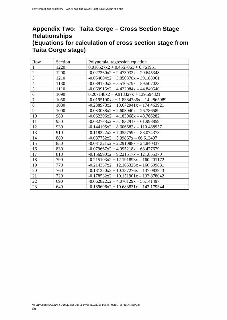
REVISION OF THE NUMERICAL MODEL FOR THE LOWER HUTT GROUNDWATER ZONE
WELLINGTON REGIONAL COUNCIL, RESOURCE INVESTIGATIONS DEPARTMENT, TECHNICAL REPORT
68
Appendix Two: Taita Gorge – Cross Section StageRelationships(Equations for calculation of cross section stage fromTaita Gorge stage)
Row Section Polynomial regression equation1 1220 0.010527x2 + 0.455706x + 6.7619512 1200 -0.027360x2 + 2.473033x – 20.6453483 1210 -0.054004x2 + 3.850378x – 39.1889614 1130 -0.089150x2 + 5.510579x – 59.5070235 1110 -0.069915x2 + 4.422984x – 44.8495406 1090 0.207148x2 – 9.918327x + 139.5943217 1050 -0.0195190x2 + 1.8384786x – 14.28659898 1030 -0.238973x2 + 13.672941x – 174.4639219 1000 -0.033038x2 + 2.603040x – 26.78658910 980 -0.062306x2 + 4.183068x – 48.76628211 950 -0.082783x2 + 5.183291x – 61.99885912 930 -0.144105x2 + 8.606582x – 110.48895713 910 -0.118322x2 + 7.055759x – 88.07437314 880 -0.087752x2 + 5.39867x – 66.61249715 850 -0.031321x2 + 2.291088x – 24.84033716 830 -0.079667x2 + 4.995218x – 63.47767917 810 -0.156990x2 + 9.221517x – 121.85537018 790 -0.215103x2 + 12.191893x – 160.20117219 770 -0.214337x2 + 12.165325x – 160.60983120 760 -0.181220x2 + 10.387276x – 137.08394321 720 -0.178532x2 + 10.151901x – 133.87804222 690 -0.062822x2 + 4.076129x – 55.14149723 640 -0.189696x2 + 10.683831x – 142.179344

REVISION OF THE NUMERICAL MODEL FOR THE LOWER HUTT GROUNDWATER ZONE
WELLINGTON REGIONAL COUNCIL, RESOURCE INVESTIGATIONS DEPARTMENT, TECHNICAL REPORT
69
Appendix Three: Stage – Wetted PerimeterRelationships for River Model Cells
Model Row 1X Section 1220
Model Row 2X Section 1200
Model Row 3X Section 1170
y = -0.875758x4 + 95.065346x3 - 3866.112179x2 + 69815.211927x - 472310.906934R2 = 0.978107
0
10
20
30
40
50
60
70
80
24 25 26 27 28 29 30stage (m amsl)
wet
ted
oerim
eter
(m)
1998
y = -0.6459207x4 + 67.9735043x3 - 2678.5502914x2 + 46849.8207848x - 306870.2740093R2 = 0.9853526
0
10
20
30
40
50
60
70
80
90
23 24 25 26 27 28 29
stage (m amsl)
wet
ted
perim
eter
(m)
1998

REVISION OF THE NUMERICAL MODEL FOR THE LOWER HUTT GROUNDWATER ZONE
WELLINGTON REGIONAL COUNCIL, RESOURCE INVESTIGATIONS DEPARTMENT, TECHNICAL REPORT
70
Model Row 4X Section 1130
Model Row 5X Section 1110
Model Row 6X Section 1090
y = -0.5891026x4 + 60.9983489x3 - 2365.7122232x2 + 40734.0586587x - 262702.5277095R2 = 0.9885477
0
10
20
30
40
50
60
70
80
90
20 22 24 26 28 30stage (m amsl)
wet
ted
perim
eter
(m)
1998
y = -0.51474x4 + 51.94414x3 - 1961.14286x2 + 32843.88488x - 205860.13039R2 = 0.99375
0
20
40
60
80
100
120
140
20 22 24 26 28 30stage (m amsl)
wet
ted
perim
eter
(m)
1998
y = -0.23015x4 + 23.82911x3 - 922.67074x2 + 15849.79229x - 101899.15974R2 = 0.99325
0
20
40
60
80
100
120
140
160
180
20 22 24 26 28 30stage (m amsl)
wet
ted
perim
eter
(m)
1998

REVISION OF THE NUMERICAL MODEL FOR THE LOWER HUTT GROUNDWATER ZONE
WELLINGTON REGIONAL COUNCIL, RESOURCE INVESTIGATIONS DEPARTMENT, TECHNICAL REPORT
71
Model Row 7X Section 1050
Model Row 8X Section 1030
Model Row 9X Section 1000
y = -0.380570x4 + 37.395653x3 - 1373.850250x2 + 22380.827873x - 136398.292825R2 = 0.990931
0
20
40
60
80
100
120
140
160
180
20 21 22 23 24 25 26 27 28stage (m amsl)
wet
ted
perim
eter
(m)
1998
y = -0.941783x4 + 83.411959x3 - 2763.435766x2 + 40598.754877x - 223146.547154R2 = 0.996474
0
20
40
60
80
100
120
20 21 22 23 24 25stage (m amsl)
wet
ted
perim
eter
(m)
1998
y = 0.113122x4 - 9.207351x3 + 276.116238x2 - 3588.549178x + 16976.404203R2 = 0.9691720
20
40
60
80
100
120
140
160
180
200
20 21 22 23 24 25 26stage m amsl
wet
ted
perim
eter
m
1998

REVISION OF THE NUMERICAL MODEL FOR THE LOWER HUTT GROUNDWATER ZONE
WELLINGTON REGIONAL COUNCIL, RESOURCE INVESTIGATIONS DEPARTMENT, TECHNICAL REPORT
72
Model Row 10X Section 980
Model Row 11X Section 950
Model Row 12X Section 930
y = -0.161785x4 + 14.049694x3 - 453.442447x2 + 6461.149321x - 34279.043502R2 = 0.998230
0
20
40
60
80
100
120
140
160
180
200
20 21 22 23 24 25 26stage m amsl
wet
ted
perim
eter
m
1998
y = 0.463869x4 - 32.560218x3 + 845.917832x2 - 9599.255633x + 39976.377040R2 = 0.979744
0
20
40
60
80
100
120
140
16 17 18 19 20 21 22stage m amsl
wet
ted
perim
eter
m
1998
y = -8.8095x2 + 337.26x - 3100.4R2 = 0.9945
0
20
40
60
80
100
120
140
15.5 16 16.5 17 17.5 18 18.5 19 19.5stage mamsl
wet
ted
perim
eter
, m
1998

REVISION OF THE NUMERICAL MODEL FOR THE LOWER HUTT GROUNDWATER ZONE
WELLINGTON REGIONAL COUNCIL, RESOURCE INVESTIGATIONS DEPARTMENT, TECHNICAL REPORT
73
Model Row 13X Section 910
Model Row 14X Section 880
Model Row 15X Section 850
y = 1.324009x4 - 87.797980x3 + 2172.428904x2 - 23748.248640x + 96745.363636R2 = 0.983116
0
20
40
60
80
100
120
140
13 14 15 16 17 18 19 20stage, mamsl
wet
ted
perim
eter
, m
1998
y = -1.006993x4 + 68.068376x3 - 1720.032634x2 + 19270.943279x - 80742.090909R2 = 0.986837
0
20
40
60
80
100
120
140
13 14 15 16 17 18 19 20stage, mamsl
wet
ted
perim
eter
, m
1998
y = 0.135198x4 - 7.569542x3 + 153.672494x2 - 1304.597125x + 3785.692308R2 = 0.994358
0
20
40
60
80
100
120
140
160
12 13 14 15 16 17 18
stage, m amsl
wet
ted
perim
eter
, m
1998

REVISION OF THE NUMERICAL MODEL FOR THE LOWER HUTT GROUNDWATER ZONE
WELLINGTON REGIONAL COUNCIL, RESOURCE INVESTIGATIONS DEPARTMENT, TECHNICAL REPORT
74
Model Row 16X Section 830
Model Row 17X Section 810
Model Row 18X Section 790
y = -1.082751x4 + 67.163559x3 - 1554.171037x2 + 15931.163073x - 61019.510489R2 = 0.995231
0
50
100
150
200
250
12 13 14 15 16 17 18 19stage, mamsl
wet
ted
perim
eter
, m
1998
y = 0.046560x4 - 1.949423x3 + 28.144953x2 - 118.409981x - 179.272165R2 = 0.988516
0
50
100
150
200
250
10 11 12 13 14 15 16 17stage, mamsl
wet
ted
perim
eter
, m
1998
y = -0.069930x4 + 4.644911x3 - 106.262238x2 + 1050.272339x - 3817.144522R2 = 0.987700
0
20
40
60
80
100
120
140
160
180
8 9 10 11 12 13 14 15 16stage, mamsl
wet
ted
perim
eter
, m
1998

REVISION OF THE NUMERICAL MODEL FOR THE LOWER HUTT GROUNDWATER ZONE
WELLINGTON REGIONAL COUNCIL, RESOURCE INVESTIGATIONS DEPARTMENT, TECHNICAL REPORT
75
Model Row 19X Section 770
Model Row 20X Section 760
Model Row 21X Section 720
y = 0.069579x5 - 3.736646x4 + 77.960484x3 - 788.343924x2 + 3876.601108x - 7458.591185R2 = 0.966064
0
20
40
60
80
100
120
7 8 9 10 11 12 13 14
stage, mamsl
wet
ted
perim
eter
, m
1998
y = -0.523927x4 + 24.017962x3 - 405.699541x 2 + 3031.885443x - 8483.354645R2 = 0.993710
0
50
100
150
200
250
300
8 9 10 11 12 13 14 15 16
stage, mamsl
wet
ted
perim
eter
, m
1998
y = 1.286713x4 - 56.385392x3 + 916.205128x2 - 6511.651904x + 17083.863636R2 = 0.991900
0
20
40
60
80
100
120
140
7 8 9 10 11 12 13stage, mamsl
wet
ted
perim
eter
, m
1998
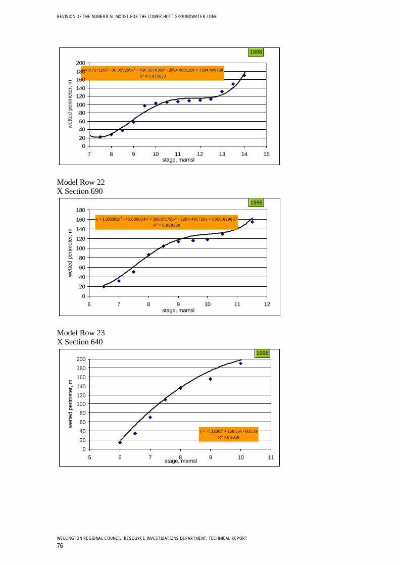
REVISION OF THE NUMERICAL MODEL FOR THE LOWER HUTT GROUNDWATER ZONE
WELLINGTON REGIONAL COUNCIL, RESOURCE INVESTIGATIONS DEPARTMENT, TECHNICAL REPORT
76
Model Row 22X Section 690
Model Row 23X Section 640
y = 0.727120x4 - 30.055265x3 + 456.367030x2 - 2994.083118x + 7184.409768R2 = 0.975633
020
4060
80100
120140
160180
200
7 8 9 10 11 12 13 14 15stage, mamsl
wet
ted
perim
eter
, m
1998
y = 1.305361x4 - 45.830614x3 + 590.871795x2 - 3284.495726x + 6658.829837R2 = 0.989389
0
20
40
60
80
100
120
140
160
180
6 7 8 9 10 11 12stage, mamsl
wet
ted
perim
eter
, m
1998
y = -7.1286x2 + 158.56x - 685.39R2 = 0.9858
0
20
40
60
80
100
120
140
160
180
200
5 6 7 8 9 10 11stage, mamsl
wet
ted
perim
eter
, m
1998