review on linear algebra essentials dr.ilkay - metu

AE 483 Automatic Control Systems II

METU, Department of Aerospace Engineering

1

REVIEW ON LINEAR ALGEBRA ESSENTIALS

Dr.Ilkay Yavrucuk

VECTOR SPACES

Def: A vector space V is a set of objects, called vectors, for which operations of vector

addition and scalar multiplication are defined.

e.g.

R1 is a vector space “line”

R2 is the usual “x-y plane”

R3 is the “3-D space”

In a vector space the following has to be satisfied (for x and y being vectors,

c1 and

c2 being

scalars):

1) x+y = y+x

2) x+(y+z) = (x+y)+z

3) There is a unique “zero vector” that satisfies x+0 = x, for all x

4) For each x there is a unique vector –x such that x+(-x) = 0

5) 1x = x

6)

(c1c2)x c1(c2x)

7)

c(x y) cx cy

8)

(c1 c2)x c1x c2x

e.g.

V Rn is a vector space

Def: A subspace of a vector space is a non-empty subset that satisfies two requirements:

1) if we add two vectors in the subspace, their sum x+y remains in the subspace;

2) if we multiply any vector x in the subspace by any scalar c, the multiplication cx

is still in the subspace.

Def: Let V be a vector space and .

1) are linearly dependent if there is a set of scalars

with at least one non-zero scalar, for which

(1)



2

,

We say is a linear combination of vectors . For a set of vectors to

be linearly dependent one of them must be a linear combination of the others.

2) If the only solution for eqn.(1) is

→ are linearly independent.

3) Def: is called a basis for V if for every there is a unique

choice of scalars , for which

This implies that are independent.

Def: If such a basis exists, then V is called a finite dimensional, otherwise it is

infinite dimensional.

If V is a vector space with a basis , then every basis for V will contain

exactly m vectors. The number “m” is called the dimension of V.

MATRICES AND LINEAR SYSTEMS

Def: Matrices are rectangular arrays of real or complex numbers; in general matrix of order

has a form:

A matrix of order “n” is shorthand for square matrix of order.

Def:

1) Let A and B be of order , then the sum of A and B is the matrix C = A+B of

order ,

2) Let be a scalar. Then the scalar multiplication is of order and

3) Let and , then the product is such that



3

4) Let . The transpose has the order such that

Some properties of square matrices:

1) A+B = B+A

2) (A+B)+C = A+(B+C)

3) A(B+C) = AB+AC

4) A(BC) = (AB)C

5)

6)

Def: A zero matrix of order has all its entries equal to zero, and is denoted by

or simply O.

For any , A+O = O+A = A.

Def: The identity matrix of order n is defined by

,

, for all , .

For all matrices and , AI = A, IB = B.

Def: Let A be a square matrix of order n. If there is a square matrix B of order n, for which

AB = BA = I, then we say A is invertible. It can be shown that matrix B is unique, but might

not always exist. It is denoted as . So, the matrix A is called invertible if exists.

Remark: If A and B are invertible, then

Def: A matrix A is called symmetric if . The matrix A is skew-symmetric if

. All symmetric and skew-symmetric matrices are also square.

Def: Let matrix A be of order . The row-rank of A is the number of linearly

independent rows. The column-rank of A is the number of linearly independent columns.

Theorem: Let be a square matrix with elements from R and let the vector space be

. Then following are equivalent statements:

1) Ax = b has a unique solution for any



4

2) Ax = 0 has a unique solution x = 0

3) exists

4)

5) full rank

Def: The nullspace of a matrix A consists of all vectors x such that Ax = 0 and . It is

denotes by N(A). The nullspace is a subspace.

DETERMINANTS

Def: The determinant of matrix A is a combination of row i and the cofactors of row i:

The cofactor is the determinant of :

.

is formed by deleting row i and column j of A.

Some Properties of Determinants:

1) det(tA) = tdet(A)

2) det(I) = 1

3) If two rows are equal, det(A) = 0

4) Elementary matrix operations do not change determinants

5) If A has a zero row, det(A) = 0

6) If is a triangular matrix,

7) If det(A) = 0, then A is called singular matrix.

8) det(A∙B) = det(A) ∙det(B)

9)

EIGENVALUES AND EIGENVECTORS

Def: The number , complex or real, is an eigenvalue of the square matrix A if there is a

vector , such that



5

The vector x is called an eigenvector corresponding to the eigenvalue .

Example:

Consider the following initial value problem:

This is an initial value problem. The unknown are specified at time t = 0, and not at both

points of the interval.

In a matrix form the system can be written as:

, ,

.

Where u is the unknown vector, - its initial value, A – coefficient matrix.

In this notation, the system becomes a vector equation

Note that it is a first-order linear equation with constant coefficients; the matrix A is time

independent.

Rewrite this equation in a scalar form:

The solution is:

Thus the initial condition and the equation are both satisfied.

for , the system is unstable;

for , the system is stable;

for , the system is neutrally stable.

If is a complex number, ,



6

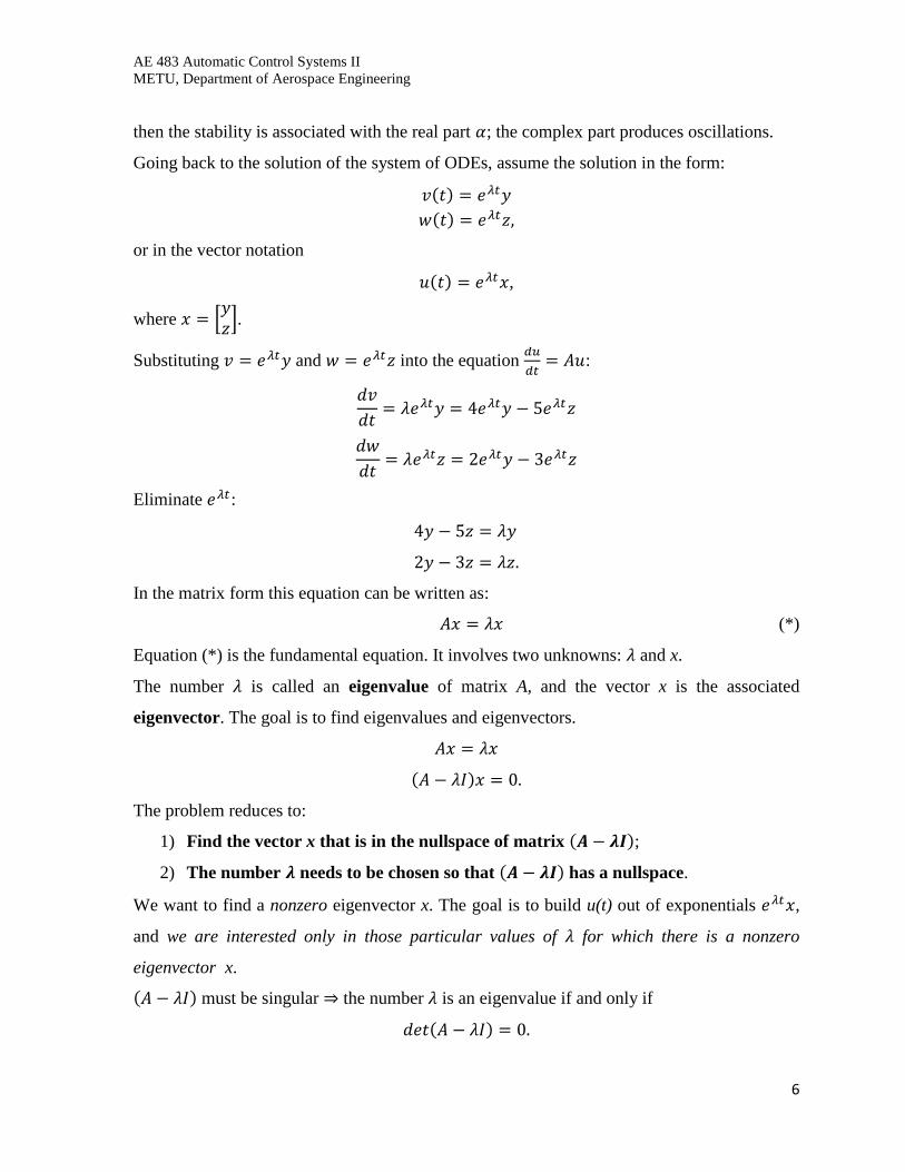
then the stability is associated with the real part ; the complex part produces oscillations.

Going back to the solution of the system of ODEs, assume the solution in the form:

or in the vector notation

,

where .

Substituting and into the equation

:

Eliminate :

In the matrix form this equation can be written as:

(*)

Equation (*) is the fundamental equation. It involves two unknowns: and x.

The number is called an eigenvalue of matrix A, and the vector x is the associated

eigenvector. The goal is to find eigenvalues and eigenvectors.

The problem reduces to:

1) Find the vector x that is in the nullspace of matrix ;

2) The number needs to be chosen so that has a nullspace.

We want to find a nonzero eigenvector x. The goal is to build u(t) out of exponentials ,

and we are interested only in those particular values of for which there is a nonzero

eigenvector x.

must be singular the number is an eigenvalue if and only if



7

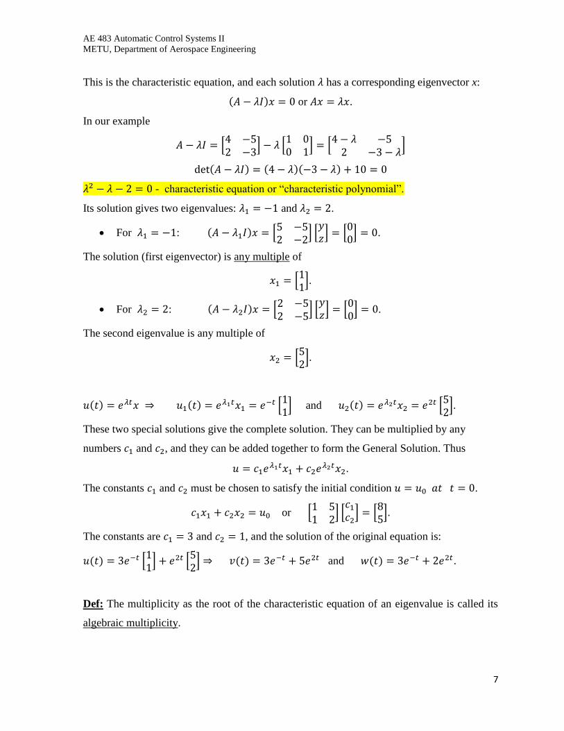
This is the characteristic equation, and each solution has a corresponding eigenvector x:

or .

In our example

- characteristic equation or “characteristic polynomial”.

Its solution gives two eigenvalues: and .

For :

.

The solution (first eigenvector) is any multiple of

.

For :

.

The second eigenvalue is any multiple of

.

and

.

These two special solutions give the complete solution. They can be multiplied by any

numbers and , and they can be added together to form the General Solution. Thus

.

The constants and must be chosen to satisfy the initial condition .

or

.

The constants are and , and the solution of the original equation is:

and .

Def: The multiplicity as the root of the characteristic equation of an eigenvalue is called its

algebraic multiplicity.



8

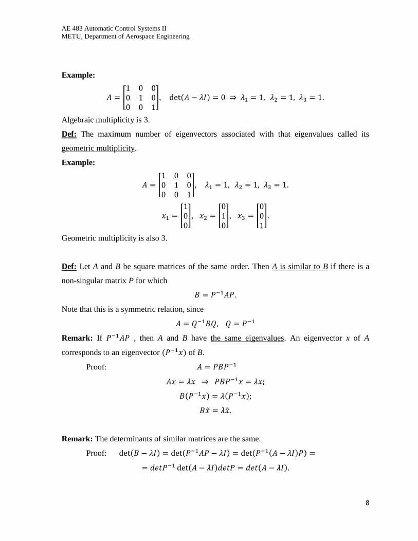
Example:

, .

Algebraic multiplicity is 3.

Def: The maximum number of eigenvectors associated with that eigenvalues called its

geometric multiplicity.

Example:

, .

,

,

.

Geometric multiplicity is also 3.

Def: Let A and B be square matrices of the same order. Then A is similar to B if there is a

non-singular matrix P for which

.

Note that this is a symmetric relation, since

Remark: If , then A and B have the same eigenvalues. An eigenvector x of A

corresponds to an eigenvector of B.

Proof:

Remark: The determinants of similar matrices are the same.

Proof:



9

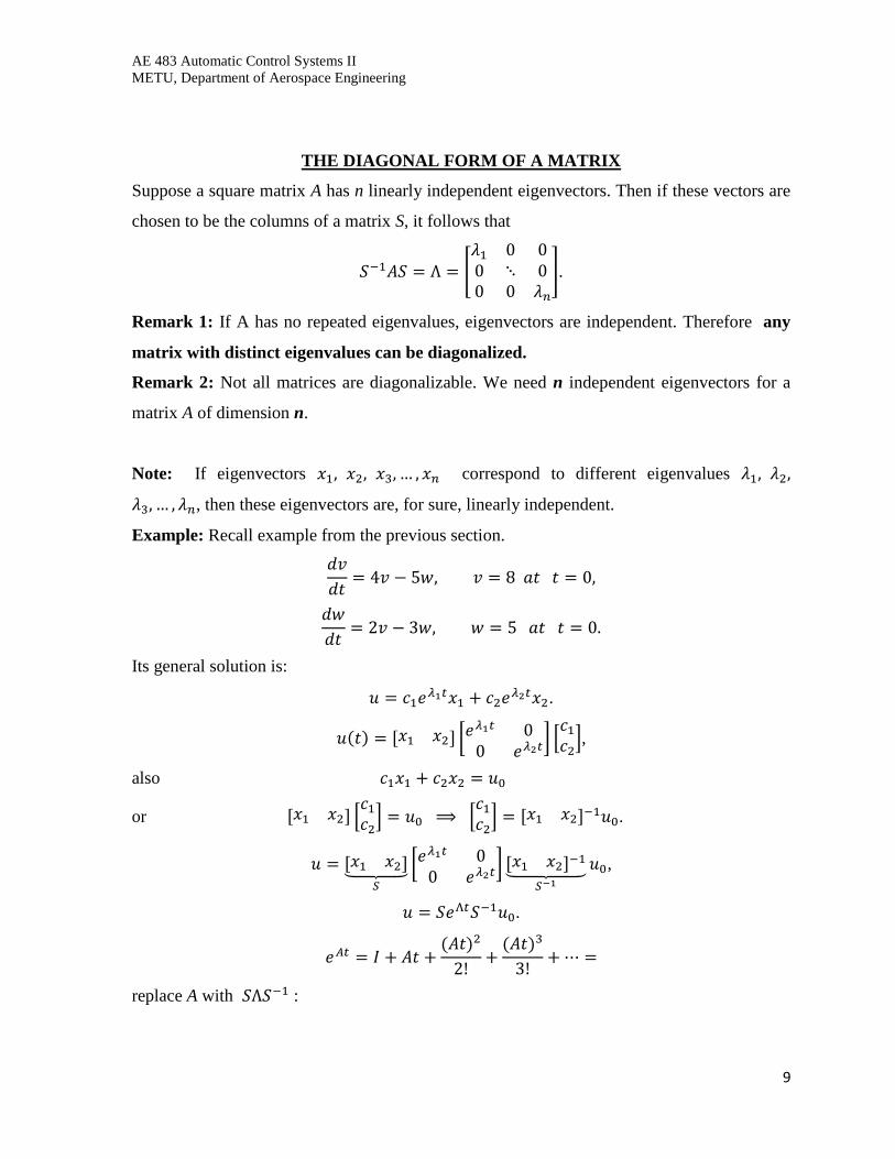
THE DIAGONAL FORM OF A MATRIX

Suppose a square matrix A has n linearly independent eigenvectors. Then if these vectors are

chosen to be the columns of a matrix S, it follows that

.

Remark 1: If A has no repeated eigenvalues, eigenvectors are independent. Therefore any

matrix with distinct eigenvalues can be diagonalized.

Remark 2: Not all matrices are diagonalizable. We need n independent eigenvectors for a

matrix A of dimension n.

Note: If eigenvectors correspond to different eigenvalues

, then these eigenvectors are, for sure, linearly independent.

Example: Recall example from the previous section.

Its general solution is:

.

,

also

or

.

,

.

replace A with :



10

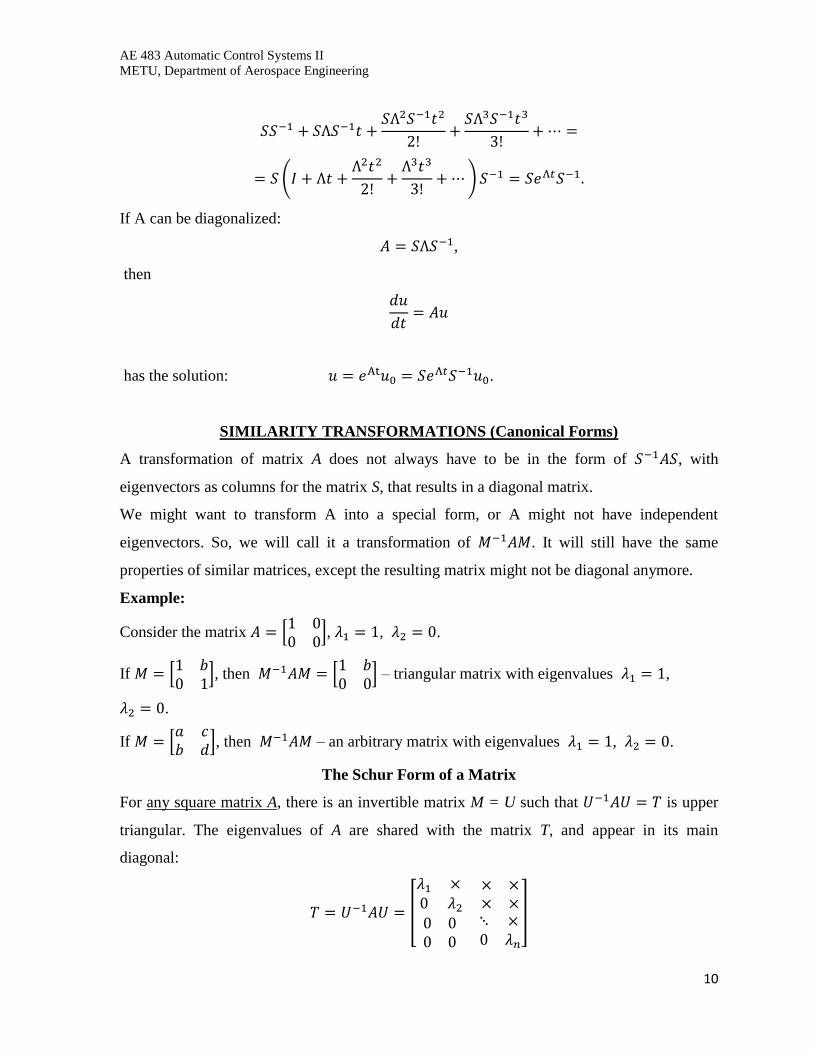
If A can be diagonalized:

,

then

has the solution: .

SIMILARITY TRANSFORMATIONS (Canonical Forms)

A transformation of matrix A does not always have to be in the form of , with

eigenvectors as columns for the matrix S, that results in a diagonal matrix.

We might want to transform A into a special form, or A might not have independent

eigenvectors. So, we will call it a transformation of . It will still have the same

properties of similar matrices, except the resulting matrix might not be diagonal anymore.

Example:

Consider the matrix

, , .

If

, then

– triangular matrix with eigenvalues ,

.

If

, then – an arbitrary matrix with eigenvalues , .

The Schur Form of a Matrix

For any square matrix A, there is an invertible matrix M = U such that is upper

triangular. The eigenvalues of A are shared with the matrix T, and appear in its main

diagonal:



11

* There is no easy way to find T for U, but the Schur form is used in many theoretical proofs.

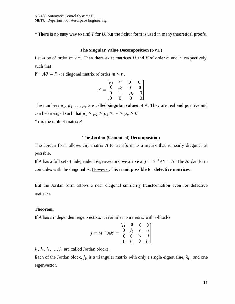
The Singular Value Decomposition (SVD)

Let A be of order . Then there exist matrices U and V of order m and n, respectively,

such that

- is diagonal matrix of order ,

The numbers , , …, are called singular values of A. They are real and positive and

can be arranged such that .

* r is the rank of matrix A.

The Jordan (Canonical) Decomposition

The Jordan form allows any matrix A to transform to a matrix that is nearly diagonal as

possible.

If A has a full set of independent eigenvectors, we arrive at . The Jordan form

coincides with the diagonal . However, this is not possible for defective matrices.

But the Jordan form allows a near diagonal similarity transformation even for defective

matrices.

Theorem:

If A has s independent eigenvectors, it is similar to a matrix with s-blocks:

, , , …, are called Jordan blocks.

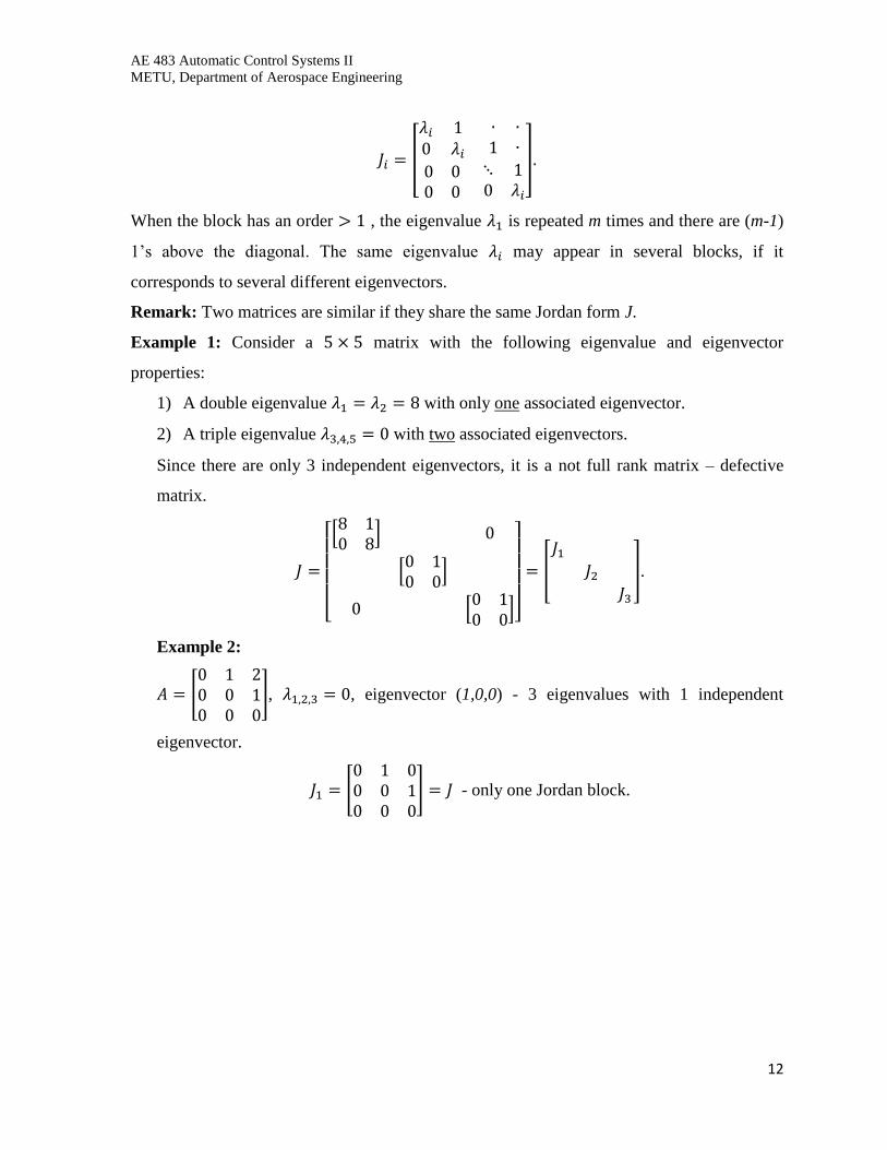
Each of the Jordan block, , is a triangular matrix with only a single eigenvalue, , and one

eigenvector,



12

When the block has an order , the eigenvalue is repeated m times and there are (m-1)

1’s above the diagonal. The same eigenvalue may appear in several blocks, if it

corresponds to several different eigenvectors.

Remark: Two matrices are similar if they share the same Jordan form J.

Example 1: Consider a matrix with the following eigenvalue and eigenvector

properties:

1) A double eigenvalue with only one associated eigenvector.

2) A triple eigenvalue with two associated eigenvectors.

Since there are only 3 independent eigenvectors, it is a not full rank matrix – defective

matrix.

.

Example 2:

, , eigenvector (1,0,0) - 3 eigenvalues with 1 independent

eigenvector.

- only one Jordan block.

review on linear algebra essentials dr.ilkay - metu

Documents