review of the washington state visibility protection state ... · pdf filereview of the...

Review of the Washington State Visibility Protection State Implementation Plan

~ Final Report ~

November 2002

02-02-012

Cover Photo: Little Annapurna peak reflected in Perfection Lake, Alpine Lakes Wilderness, Wenatchee National Forest. Photo courtesy of Gary Paull, U.S. Forest Service, Mt. Baker-Snoqualmie National Forest.

Review of the Washington State Visibility Protection State Implementation Plan

~ Final Report ~

Prepared By: Washington State Department of Ecology

Air Quality Program

November 2002 02-02-012

The Department of Ecology is an equal opportunity agency and does not discriminate on the basis of race, creed, color, disability, age, religion, national origin, sex, marital status,

disabled veteran’s status, Vietnam Era veteran’s status, or sexual orientation.

If you have special accommodation needs or require this document in alternative format, please contact Judy Beitel at (360) 407-6878 (voice) or 1-800-833-6388 (TTY

only).

Table of Contents

Page ACKNOWLEDGEMENTS ......................................................................... 1 EXECUTIVE SUMMARY .......................................................................... 2 INTRODUCTION ........................................................................................ 8 1.0 REVIEW OF MONITORING DATA FROM IMPROVE MONITORING SITES .............................................................................................11

1.1 Introduction..............................................................................................................11 1.2 Methodology............................................................................................................13 1.3 Reconstructed Mass at Mt. Rainier and Alpine Lakes.............................................18 1.4 Reconstructed Light Extinction at Mt. Rainier and Alpine Lakes...........................32 1.5 Long-term Mass and Light Extinction Trends at Mt. Rainier .................................46 1.6 Light Extinction Conditions and Trends at Other Mandatory Class I Federal Areas in the Pacific Northwest ................................................................................56 1.7 Conclusions………..………………………………………………………………60

2.0 REVIEW OF EMISSIONS DATA ................................................................62

2.1 Scope of the Emissions Inventory............................................................................62 2.2 Emissions Inventory Discussion ..............................................................................63 2.3 Conclusions..............................................................................................................70 2.4 County and Emission Zone Trends..........................................................................78

3.0 TRAJECTORY ANALYSIS............................................................................82

3.1 Introduction..............................................................................................................82 3.2 Methodology............................................................................................................83 3.3 Discussion of Trajectory Results .............................................................................84

4.0 SUMMARY OF SIP REVIEW REQUIREMENTS ..............................98

4.1 Requirement 1 – The Progress Achieved in Remedying Existing Impairment of Visibility in any Mandatory Class I Federal Area ..........................98 4.2 Requirement 2 – The Ability of the Long-term Strategy to Prevent Future Impairment of Visibility in any Mandatory Class I Federal Area ........................100 4.3 Requirement 3 - Any Change in Visibility since the Last Report ........................106 4.4 Requirement 4 - Additional Measures, Including the Need for SIP Revisions, that may Be Necessary to Assure Reasonable Progress Toward the National Visibility Goal.......................................................................................................106 4.5 Requirement 5 - The Progress Achieved in Implementing BART and Meeting

Other Schedules Set Forth in the Long-term Strategy..........................................107

4.6 Requirement 6 – The Impact of Any Exemption from BART .............................107 4.7 The Need for BART to Remedy Existing Visibility Impairment of Any

Integral Vista Listed in the Plan Since the Last Report ........................................107

5.0 CONSULTATION WITH FEDERAL LAND MANAGERS ............109 5.1 Response to USFS Comments ...............................................................................109 5.2 Response to NPS comments……………………………………………………..110 6.0 SUMMARY OF THE REGIONAL HAZE RULE AND PROGRESS TOWARDS DEVELOPING A REGIONAL HAZE SIP .............. 112

6.1 Overview…………………………………………………………………………112 6.2 Technical Activities Related to Regional Haze SIP Development………………115

7.0 RECOMMENDATIONS ................................................................................117 7.1 Recommendations on the Need to Revise the Phase I Visibility SIP……………117 7.2 Recommendations on Other Measures and Activities…………………………...117 APPENDICES

Appendix A –2002 Visibility SIP Progress Review Work Plan and the SIP Review Requirements Appendix B – Emission inventory details and methodology Appendix C – Federal Land Manager comments on Washington State’s Draft Visibility SIP Review Appendix D – Summary of the Northwest Regional Modeling Center Demonstration

Project Appendix E – Summary of the BPA Cumulative Impact Study

http://www.ecy.wa.gov/programs/air/pdfs/visSIPappendices.pdf

Acknowledgements

Ecology wishes to thank the Air Quality Group at the University of California at Davis for producing the IMPROVE data and the U.S. Forest Service, US Department of Agriculture and the National Park Service,

US Department of the Interior for funding the IMPROVE monitoring sites used in this report.

Ecology also acknowledges the following individuals who contributed to the development, preparation and review of this document.

USDI – National Park Service

Brian Mitchell Barbara Samora

USDA – Forest Service Bob Bachman

Janice Peterson US Environmental Protection Agency

Steve Body Mahbubul Islam

Washington State Department of Natural Resources Roger Autry Mark Gray

Washington State Department of Ecology Judy Beitel

Clint Bowman Michael Boyer

Mary Burg Tapas Das

Bruce Estus Elena Guilfoil Alan Newman Sandra Newton Sally Otterson

Myron Saikewicz Robert Saunders Doug Schneider

Dick Stender Frank Van Haren

Executive Summary Federal regulations and the visibility portion of Washington’s State Implementation Plan (SIP) require a formal assessment of the Visibility Protection Program every three years to determine if reasonable progress has been made and will continue to be made towards the national visibility goal. If progress cannot be demonstrated additional measures necessary to assure reasonable progress, including revisions to the SIP, must be identified. This report presents the State’s findings with respect to reasonable progress. This review was conducted in consultation with the Federal Land Manager (FLM) and is being made available to the public and the U.S. Environmental Protection Agency (EPA) to meet requirements of the federal Clean Air Act and the Washington State Visibility SIP. The national visibility goal was established in 1977 by Congress and declared: “Congress hereby declares as a national goal the prevention of any future, and the remedying of any existing impairment of visibility in mandatory Class I federal areas in which impairment results from manmade pollution” Federal strategy for visibility protection called for a two phased effort. Phase I was designed to deal with visibility impairment in mandatory Class I federal areas that is easily attributable to distinct plumes from large stationary sources and groups of stationary sources (often called “plume blight”). The control strategies in the current Washington State Visibility SIP target these kinds of sources and prescribed burning. Phase II regulations are designed to deal with visibility impairment resulting from regional haze, the wide spread impairment of visibility from the combined emissions of all sources including mobile, area, small stationary and large stationary sources. Development of phase II visibility protection regulations was forestalled until the scientific and technical limitations to understanding regional haze were overcome. EPA in consultation with states, FLMs and other stakeholders developed and promulgated the regional haze regulation in July 1999. Submission dates for regional haze SIPs are tied to PM2.5 designations, which are expected to occur by the end of 2004. Washington State anticipates the completion and submission of its first regional haze SIP will occur between 2006 and 2008. We have included a section summarizing progress to date towards developing a regional haze SIP (see section 6). The current Washington State Visibility SIP is a phase I visibility SIP. This review concerns itself mainly with those sources targeted by current control strategies. Although prescribed forestry burning is not considered a stationary source, Washington’s phase I Visibility SIP addressed this source because of the significant attributable contribution to visibility impacts from prescribed burn plumes. Control strategies in the current phase I Visibility SIP focus on three areas: 1) Smoke Management. Improved management of smoke from prescribed burning of

forest slash was the primary mechanism to improve visibility in Washington State. The Smoke Management Plan (SMP) has been revised three times to address and

Visibility SIP Review – Final Report 2

enhance protection of visibility from this source while allowing flexibility to conduct forest health burning in eastern Washington.

2) New Source Review. Visibility protection requirements were added to the state’s New Source Review (NSR) program, which requires new and modified stationary sources to mitigate any modeled impacts to visibility in mandatory Class I federal areas prior to approval of construction.

3) Best Available Retrofit Technology. A regulation to address visibility impacts from a specific subset of existing stationary sources was developed. Best Available Retrofit Technology (BART) requires control strategies on an existing stationary source to which visibility impairment in a mandatory Class I area can be reasonably attributed.

In addition to these visibility specific control strategies, the Visibility SIP relies on other ongoing air quality programs to provide improvement to visibility as a secondary benefit. The heart of a progress assessment is the analysis of mandatory Class I federal area aerosol monitoring data, source emissions data, and modeling analysis to identify geographic regions that contribute visibility impairing emissions to mandatory Class I federal areas. Major highlights of this analysis are: � Visibility impairing emissions from phase I targeted sources decreased significantly

between 1985 and 1996 (22% reduction). Phase I targeted emissions are projected to decrease another 31% by the year 2018. The total decrease in phase I targeted emissions from 1985 through 2018 is 46%. Much of the projected decrease is due to the required SO2 and NOx controls on the Centralia Power Plant.

� Between 1985 and 1996 the decrease in regional haze emissions (Phase II emissions - which include all types of sources – area, mobile, small stationary and large stationary sources) has been small but detectable (3%). From 1996 to 2018, a significant decrease (16%) is projected for regional haze emissions, most of it due to the controls on the Centralia Power Plant and mobile sources.

� Individual county emissions were analyzed and all counties except Pend Oreille projected a decrease in visibility impairing emissions. The increase in Pend Oreille county emissions was less than 1%.

� Three geographic emission zones were delineated to represent areas where emissions could reasonably be expected to affect one or more mandatory Class I federal areas. Each emission zone showed significant projected regional haze emissions decrease from 1996 to 2018, ranging from 16% to 23% decrease. � The emission zone representative of Mt. Rainier showed a projected emission

decrease through 2018 at a rate that would lead to natural conditions by the year 2064, if that rate were to continue. However, actual emission levels after the year 2018 were not estimated at this time, and it is unknown if this rate will continue without additional strategies.

� An important caveat is that an assumption is made that there is a 1:1 relationship between emissions reduced and light extinction reduced (visibility improved). This is a conservative assumption because under normal Pacific Northwest conditions pollutant species cause more light extinction then their unadjusted dry masses would allow. Therefore, reducing emissions should actually cause more


reduction in light extinction then a 1:1 ratio. Nonetheless, it is important to note that air quality levels resulting from the projected emission reductions were not modeled.

� There is an increase projected in emissions from prescribed burning to protect forest health in eastern Washington. However, this increase is not enough to overcome the net decrease expected from all emissions combined.

� Aerosol monitoring data were analyzed at two Washington sites – Mt. Rainier National Park and Alpine Lakes Wilderness. � Trends in reconstructed light extinction for the best case, average and worst case

days showed a statistically significant decreasing trend (improving visibility) at Mt. Rainier for the period 1989 to 1999.

� However, closer examination of recent trends (1995 - 1999) indicates that there is no statistically significant trend in either direction for this more recent period.

� Not enough years meet minimum data completeness to determine a trend at Alpine Lakes.

� No data existed to make a trends determination about the other 6 mandatory Class I federal areas of Washington, as monitoring was only recently established.

� At both monitoring sites most of the worst case days occur in summer; most of the best case days occur in winter.

� A closer look at individual pollutant species contributing to light extinction indicates that all species except soil showed a statistically significant decreasing trend at Mt. Rainier. However, the decrease in nitrate may be due to a monitoring protocol change made in 1996.

� In all cases at both sites reconstructed light extinction is dominated by sulfate followed by organic carbon.

� At Mt. Rainier, reconstructed light extinction levels range from 17.04 Mm-1 for the best case days (natural conditions are estimated at 13.14 Mm-1) to 69.25 Mm-1 for the worst case days.

� At Alpine Lakes reconstructed light extinction levels range from 18.45 Mm-1 for the best case days (natural conditions are estimated at 13.00 Mm-1) to 61.48 Mm-1 for the worst case days.

� Using the method prescribed by the regional haze rule, the trend in visibility at Mt. Rainier is estimated to be improving for the period 1989 - 1999 at a rate that would lead to natural conditions by the year 2064, if that rate were to continue. Actual visibility levels after the year 1999 cannot be predicted at this time, although it is assumed visibility will continue to improve because of the projected emission reductions through the year 2018. It is unknown whether this improving trend will continue after 2018.

� Trajectory analysis indicates there are definite seasonal patterns of air masses bringing pollutants to the two monitoring sites – Mt. Rainier and Alpine Lakes.

� There are also definite trajectory patterns on the worst case visibility days that indicate trajectories for both sites spend a large fraction of time over the populated areas of the Puget Sound. This fact may have air management implications on the Puget Sound region should additional control strategies be deemed necessary in the future.


� Two other mandatory Class I area aerosol monitoring sites outside of Washington State were analyzed for comparison purposes only. The two sites were Three Sisters Wilderness in Oregon and Glacier National Park in Montana. � Light extinction levels at these sites were similar to those in Washington,

although individual pollutant species contribution to light extinction was different from that seen at the Washington sites. Organic carbon dominated light extinction at Glacier National Park and at Three Sisters Wilderness sulfate, organic carbon and nitrate contributed to light extinction nearly equally.

� There was a statistically significant increasing trend in light extinction (worsening visibility) at Three Sisters Wilderness. Most of the increase was due to organic carbon.

� There was no statistically significant trend at Glacier National Park. Recommendations on the Need to Revise the SIP With the exception of a proposal to remove SIP review requirement 7 (see section 4.7 for a discussion), Ecology does not recommend any other revisions to the phase I Visibility SIP for the following reasons: 1. Proposed revisions to the current phase I Visibility SIP, based on recommendations

resulting from the 1997 review, have been recently recommended for approval by EPA, withstanding public comment, (See Federal Register/Volume 67, No. 205, Wednesday, 10/23/02, Proposed Rules, pg. 65077 – 65080). These revisions will result in significant additional protections for visibility by making the current Smoke Management Plan and the Centralia Power Plant RACT order federally enforceable.

2. Other work recommended by the 1997 review has been completed or is ongoing. This work has resulted in improvements to the emission inventory, modeling and monitoring. Additional improvements are ongoing or planned.

3. Current control strategies (BART, NSR, RACT, BACT, SMP and NAAQS) and national programs to reduce emissions from mobile sources, will reduce emissions or prevent future emissions that affect visibility. The goal of the visibility program is to make reasonable progress towards reaching natural conditions in mandatory Class I federal areas. We believe emission reductions resulting from these programs constitutes progress towards that goal.

4. A significant improving visibility trend was shown for Mt. Rainier for the period 1989 – 1999 (although more recent data did not show a trend in either direction).

5. Significant emission reductions from phase I targeted sources have occurred. 6. Significant emission reductions from phase I targeted sources are projected through

2018. 7. Regional haze (phase II) emissions are projected to decrease significantly through

2018. This decrease is enough to ensure reasonable progress towards the national visibility goal during the period 2000 through 2018, although emission levels after 2018 are an unknown.

8. If more emission reductions are needed in the future to maintain progress towards the visibility goal after 2018, the implementation of a regional haze SIP will address sources that are not currently targeted by the phase I Visibility SIP, such as mobile,


small stationary and area sources. Ecology will complete and submit a regional haze SIP during the 2006 to 2008 time period.

Recommendations on Other Measures and Activities The following measures and activities will improve the visibility protection program, provide a margin of safety and lead to a better understanding of haze and its effects. Implementing these measures will also help assure that in the future we continue to have an efficient, equitable and successful visibility protection program. These recommendations have significant resource implications and can only be implemented if adequate funding above and beyond current funding levels is made available. The following measures and activities are listed in descending order of priority. 1. The PSD/NSR rules require air regulatory agencies to conduct cumulative effects

analysis as part of the permit process. To date our capability to conduct cumulative effects analysis has been lacking. It is recommended that Ecology participate in developing a proposal and schedule for developing modeling capabilities to conduct cumulative effects analysis. The proposal and work involved should be a collaborative effort involving resources and expertise of the federal land manager, local air agencies, other air regulatory agencies in neighboring states, EPA, industry and Ecology. Parallel but more critical to developing technical capabilities, is the need to understand and clarify the policy and regulatory implications of cumulative effects analysis. Therefore, it is necessary that a regional policy on the use and implications of cumulative effects analysis be developed prior to the technical capabilities.

The Bonneville Power Administration recently completed a cumulative impact study of the effect of several proposed power generating facilities. Much was learned about the technical shortcomings of our ability to conduct such a study. This study could serve as a starting point for discussions. Please see Appendix E for a summary of the study.

2. Continue to support and participate in the WRAP to develop control strategies for the regional haze SIP.

3. Continue to support and participate in the Northwest Regional Modeling Center and their work in developing modeling and emission inventory capabilities for the purpose of understanding the causes and effects of haze in the Pacific Northwest.

4. The Reasonably Available Control Technology program (RACT) is designed to reduce emissions of existing stationary sources. The program allows for reducing emissions for the purpose of mitigating effects to visibility. The RACT for the Centralia Power Plant is an example of how successful this program can be for protecting and improving visibility. However, with the notable exception of the RACT for Centralia, this program has been underutilized for visibility protection. Depending on resource availability and the results of cumulative effects analysis, it is recommended that more resources be dedicated to conducting RACT analysis for all eligible sources that have been shown to impact visibility.

5. Work with EPA and the federal land manager to enhance the IMPROVE monitoring network in Washington state. The current basic network provides 24-hour average


aerosol sampling and analysis on a 1 in 3 day schedule. Additional measurement parameters such as continuous high time resolution measurements of meteorology, light scatter, light absorption and various pollutant species, would greatly increase our ability to understand the formation of haze and its effects on visibility. Additional monitoring locations to the basic network should also be considered to help us understand the transport of haze.


Introduction Purpose of the Review Federal regulations and the visibility portion of Washington’s State Implementation Plan (SIP) require a formal assessment of the Visibility Protection Program to determine if reasonable progress has been made and will continue to be made towards the national visibility goal. In 1977 Congress declared as a national visibility goal “the prevention of any future, and the remedying of any existing impairment of visibility in mandatory Class I federal areas in which impairment results from manmade pollution.” Background The federal strategy for visibility protection called for a two phased effort. Phase I was designed to deal with visibility impairment in mandatory Class I federal areas that is easily attributable to distinct plumes from large stationary sources or groups of stationary sources (often called “plume blight”). The control strategies found in the current Washington State Visibility SIP target these kinds of sources and prescribed burning. Although prescribed forestry burning is not considered a stationary source, Washington’s phase I Visibility SIP addressed this source because of the significant attributable contribution to impacts from prescribed burn plumes. Phase II regulations are designed to deal with visibility impairment resulting from regional haze, the wide spread impairment of visibility from the combined emissions of all sources including mobile, area, small stationary sources and urban plumes. Development of phase II visibility protection regulations was forestalled until the scientific and technical limitations to understanding regional haze were overcome. The Washington State Department of Ecology (Ecology) submitted to the U.S. Environmental Protection Agency (EPA) revisions to the SIP for purpose of phase I visibility protection (Visibility SIP) in March 1985. EPA formally approved the Visibility SIP on May 4, 1987. Control strategies in the current phase I Visibility SIP focus on three areas: 1) Smoke Management. Improved management of smoke from prescribed burning of

forest slash was the primary mechanism to improve visibility in Washington State. The Smoke Management Plan (SMP) has been revised three times to address and enhance protection of visibility from this source while allowing flexibility to conduct forest health burning in eastern Washington.

2) New Source Review. Visibility protection requirements were added to the state’s New Source Review (NSR) program, which requires new and modified stationary sources to mitigate any modeled impacts to visibility in mandatory Class I federal areas prior to approval of construction.

3) Best Available Retrofit Technology. A regulation to address visibility impacts from a specific subset of existing stationary sources was developed. Best Available Retrofit Technology (BART) requires control strategies on any existing stationary source to which visibility impairment in a mandatory Class I area can be reasonably attributed.

In addition to these visibility specific control strategies, the Visibility SIP relies on other ongoing air quality programs to provide secondary benefits to visibility. These programs


include Reasonably Available Control Technology, Best Available Control Technology, local and state programs to meet the National Ambient Air Quality Standards and national air quality programs to reduce emissions from mobile sources. In accordance with federal regulations, the Visibility SIP called for a formal review of progress every three years from the date of adoption by EPA. The first review of the Visibility SIP was completed in April of 1997 (see Review of the Washington State Visibility Protection State Implementation Plan – Final Report, April 1997, Ecology publication No. 97-206). The review recommended several revisions to the Visibility SIP. Revisions based on the 1997 SIP review were submitted to EPA in September 1999. Major revisions include incorporating the updated Smoke Management Plan and the RACT order for the Centralia coal fired power plant. EPA recently recommended for approval most of the proposed revisions except BART and NSR as these rules are undergoing further revision by the State, (See Federal Register/Volume 67, No. 205, Wednesday, 10/23/02, Proposed Rules, pg. 65077 – 65080). A second review was conducted in 1999. The 1999 Visibility SIP review did not recommend any additional revisions to the SIP. Reasons for not recommending revisions was that significant progress had been made in reducing light extinction and significant reductions of visibility impairing emissions had occurred and were anticipated to continue (see Review of the Washington State Visibility Protection State Implementation Plan – Final Report, July 1999, Ecology publication No. 99-206). This document constitutes the third periodic review. EPA in consultation with states, the Federal Land Managers (agencies responsible for the management of national parks and wilderness areas) and other stakeholders developed and promulgated the regional haze rule in July 1999. Washington State anticipates completion and submission of its first regional haze SIP will occur between 2006 and 2008. Process and Scope of the Review This review report is the result of consultation with stakeholders during the Visibility SIP review process. Ecology began the consultation process in the winter of 2001/2002 by forming a work group of staff from Ecology, FLMs, EPA and state land managers. A series of meetings and discussions took place over a three-month period that tapped the expertise in each of these agencies and culminated in the development of a SIP review work plan. The work plan spelled out the specifics of how the evaluation for each SIP review requirement would be conducted. The work plan and SIP review requirements can be found in Appendix A. In addition to consultation before and during the SIP review process, Ecology prepared and distributed to the FLMs a Federal Land Manager Review Draft and asked the FLM to prepare written comments. Although these agencies were consulted in the process and contributed to the development of the final report, all views, opinions, conclusions


and recommendations are solely those of the Washington State Department of Ecology, unless otherwise noted. This report is divided into seven sections plus appendices. The first three sections present and discuss results from the technical analysis that was conducted to form the foundation for the assessment of reasonable progress (as required for SIP review requirements 1 through 4). Section 4 summarizes our conclusions with respect to the SIP review requirements. Section 5 is a discussion of Ecology’s consultation with the FLM and our response to their comments on the draft SIP Review Report. Section 6 summarizes the regional haze rule and progress towards developing a regional haze SIP. And lastly, section 7 discusses recommendations resulting from this Visibility SIP review.


1.0 REVIEW OF MONITORING DATA FROM IMPROVE MONITORING SITES 1.1 Introduction Background Interagency Monitoring of Protected Visual Environments (IMPROVE) monitoring is conducted across the nation at several visually important Class I and Class II areas. The IMPROVE monitoring network, monitoring methodology and data analysis methodology has been developed over several years by a consortium of scientists from the EPA, FLMs, states groups and academia. The IMPROVE protocol for visibility monitoring and analysis represents the current state of the art in visibility monitoring science and is routinely used by those interested in visibility conditions throughout the United States. IMPROVE visibility monitoring is being conducted at several locations in Washington State, however only two Class I area sites have a sufficiently long, uninterrupted, year round monitoring record to be useful for this review. Mt. Rainier National Park IMPROVE monitoring has been conducted on a year-round basis since the spring of 1988. IMPROVE monitoring at Alpine Lakes Wilderness has been conducted on a year-round basis since the fall of 1994. IMPROVE aerosol data from Mt. Rainier National Park (near Ashford) and Alpine Lakes Wilderness (at Snoqualmie Pass) are used for all analysis with respect to progress made in Washington, unless otherwise noted. Note: Four additional Class I area IMPROVE sites have recently been established, but to date no data from these sites is available for analysis. Therefore, analysis is limited to Mt. Rainier and Alpine Lakes. For additional details on the expanded IMPROVE network, please see section 6.2. It should be noted that data completeness for the Alpine Lakes site is significantly low. Essentially, only two years of data from the historical data set meet the completeness criteria outlined in the “Draft Guidance for Tracking Progress Under the Regional Haze Rule”, (USEPA). That criteria is no less than 75% per year, 50% for any season and no more than 10 consecutive missing days in any season. Even after eligible data substitutions were made only the years 1997 and 1998 met the completeness criteria. Only those two years will be used in the analysis for Alpine Lakes. In addition to the Mt. Rainier and Alpine Lakes sites, IMPROVE data from nearby out-of-state mandatory Class I federal areas were analyzed. This data is used for comparison purposes only. These sites are: � Glacier National Park in Montana (Class I area site) � Three Sisters Wilderness in Oregon (Class I area site). This site actually represents

three mandatory Class I federal areas in Oregon: Mt. Jefferson, Mt. Washington and Three Sisters Wilderness.

Monitoring and data analysis protocol used for these sites is the same as that used for Mt. Rainier and Alpine Lakes. Figure 1.1 shows the locations of the four monitoring sites


analyzed for this review. Table 1.1 lists site location coordinates and elevations. All sites meet the IMPROVE monitoring siting criteria as contained in “IMPROVE Particulate Monitoring Network Procedures for Site Selection” (UC Davis). This document can be accessed at the NPS Visibility Monitoring website (http://www2.nature.nps.gov/ard/vis/vishp.html). For a closer look at local terrain of the sites, it is recommended that the reader visit the Topozone website (http://www.topozone.com/). In the “Get a Map” section, click on “decimal degrees” and enter the coordinates. Figure 1.1 Locations of IMPROVE monitoring sites used in this report Table 1.1 Location coordinates and elevations of IMPROVE sites used in this report Station

Code Start date Longitude

(decimal degrees)

Latitude (decimal degrees)

Elevation (meters)

Mt. Rainier MORA1 3/2/88 -122.1225 46.7579 427 Alpine Lakes SNPA1 7/3/93 -121.4277 47.4203 1160 Glacier GLAC1 3/2/88 -113.9966 48.5104 979 Three Sisters THSI1 7/24/93 -122.0432 44.291 885


http://www2.nature.nps.gov/ard/vis/vishp.html)

Purpose The purpose of this data analysis section is to characterize current annual and seasonal levels of visibility at the two long-term Washington State IMPROVE sites, compare visibility at the two sites, identify those pollutants that have a negative effect on visibility at these sites and define the long-term trends in visibility. This analysis, along with the emissions analyses presented in section 2, forms the technical foundation upon which Ecology has based its conclusions with respect to reasonable progress. Fine (PM2.5) and coarse (PM10) particulate mass are measured directly at both sites. Fine mass is also reconstructed using speciated chemical data. The fine mass species used for this analysis are sulfate, nitrate, organic carbon, elemental carbon, and soil. In addition, non-speciated coarse mass is reported. These species, which are responsible for light extinction, are measured at visibility monitoring sites across the nation. The individual species masses are summed to obtain reconstructed total mass (RTM) and reconstructed fine mass (RFM). Light extinction is the ability of particles and gases in the atmosphere to absorb and scatter light. Because light extinction is dominated by the effects of particles, light extinction by gasses is not routinely measured. Light extinction can be measured directly using continuous monitors or it can be reconstructed from twice weekly, 24-hour averaged speciated chemical data. Reconstructed light extinction is the sum of the light extinction coefficient of each species mentioned above multiplied by the ambient mass concentration of each species. Some species are hygroscopic (sulfate and nitrate), meaning that their ability to scatter light is dependent on how much moisture is present in the air. These two hygroscopic species are multiplied by a factor derived from site specific average monthly relative humidity before they are summed with the other species. Coarse mass (PM10 – PM2.5) is also measured at the sites and is combined with the reconstructed fine mass species to determine total reconstructed light extinction. Presented in this section of the Review Report are the results of the reconstruction of fine mass and light extinction to determine which particulate species are negatively affecting visibility. Section 1.2 describes the methods used to determine the aerosol mass, relative humidity factors, and reconstructed light extinction. Sections 1.3 and 1.4 present and discuss the results of aerosol mass and light extinction analysis. Section 1.5 discusses long-term trends in light extinction. Section 1.6 presents light extinction conditions and trends from two nearby mandatory Class I federal areas outside Washington State. 1.2 Methodology Sample collection and analysis The speciated chemical data used for this report was collected using the IMPROVE-protocol method, outlined in the Cooperative Institute for Research in the Atmosphere


(CIRA) report “Spatial and Seasonal Patterns and Temporal Variability of Haze and its Constituents in the United States: Report III”, Malm et al, May 2000. This method is summarized in Table 1.2. The IMPROVE-protocol sampling schedule is a 24-hr sample every Wednesday and Saturday, (note: sampling schedule was recently changed to 1 sample every 3 days). Table 1.2 Summary of Sampling and Analyses Techniques used in the IMPROVE-protocol method.

Module Filter Media Analyses A Teflon Gravimetric analysis for mass < 2.5 �m diameter

Laser Integrating Plate Method for optical absorption Particle Induced X-ray Emission for elements Na to Pb Proton Elastic Scattering for H

B Nylon (denuded) Ion Chromatography for NO3 and SO4 C Quartz Thermal Optical Reflectance for organic and elemental

carbon D Teflon Gravimetric analysis for mass < 10 �m diameter

Calculating Reconstructed Fine Mass (RFM) and Reconstructed Total Mass (RTM) The IMPROVE-protocol method measures fine particulate species by the methods described in the citation above (Malm et al). The speciated chemical data can be used to reconstruct fine and total mass. The species categories used for this analysis are sulfate, nitrate, organic carbon, elemental carbon, soil and non-speciated coarse mass. The fine mass species can be summed and compared to measured PM2.5 concentrations to see to what extent they account for fine particulate mass. The species mass concentration is denoted by [ ], and the abbreviations used are those used by the IMPROVE-method. Ecology has adopted the RFM and RTM method used by the CIRA and summarized below. Sulfate is calculated from elemental sulfur, under the assumption that all sulfur is from sulfate and all sulfate is from ammonium sulfate by the equation:

[Sulfate] = 4.125 [S] Nitrate is calculated from the nitrate ion, assuming that the denuder efficiency is close to 100% and all nitrate is from ammonium nitrate.

[Nitrate] = 1.29 [NO3] Organic carbon is calculated from the organic carbon peaks in the analysis method, assuming that the average organic molecule is 70% carbon. [Organic carbon] = 1.4 x ([O1] + [O2] + [O3] + [O4] + [OP])


Elemental carbon (also referred to as light-absorbing carbon) is calculated from the elemental carbon peaks in the analysis method, assuming all high temperature carbon is elemental and subtracting out the pyrolized carbon component. [Elemental carbon] = [E1] + [E2] + [E3] – [OP] Soil is estimated by summing the elements associated with soil, plus oxygen for the normal oxides (Al2O3, SiO2, CaO, K2O, FeO, Fe2O3, TiO2). This assumes that [Soil K] = 0.6[Fe], FeO and Fe2O3 are equally abundant, and a factor of 1.16 is used for MgO, Na2O, H2O, and CO2.

[Soil] = 2.2 [Al] + 2.49 [Si] + 1.63 [Ca] + 2.42 [Fe] + 1.94 [Ti] Once the individual species mass have been determined, they are summed to get reconstructed fine mass (RFM). RFM = [sulfate]+[nitrate]+[organic carbon]+[elemental carbon]+[soil] To calculate reconstructed total mass (RTM), coarse mass (CM) is calculated by subtracting the fine mass measurement (PM2.5) from the total mass measurement (PM10) and then summing it with the previously calculated RFM.

[CM] = [PM10] – [PM2.5] RTM = CM + RFM Calculating f(RH) As stated in the introduction to this section, some species are hygroscopic, therefore their light extinction abilities are dependent on relative humidity (RH). The Tang RH correction factor, f(RH), is used in the equation for calculating reconstructed light extinction. USEPA has developed a set of monthly average f(RH) factors for all monitoring locations in the nation and reported these factors in “Draft Guidance for Tracking Progress Under the Regional Haze Rule”, USEPA, September 27 2001. Table 1.3 lists the monthly f(RH) factors for sites used in this review. Seasonal average f(RH) are also listed in table 1.3. Seasons are defined as: � Summer, 6/1 – 8/31 � Fall, 9/1 – 11/30 � Winter, 12/1 – 2/28 � Spring, 3/1 – 5/31


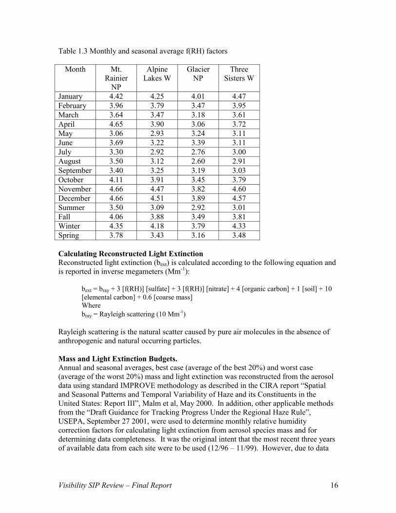
Table 1.3 Monthly and seasonal average f(RH) factors

Month Mt. Rainier

NP

Alpine Lakes W

Glacier NP

Three Sisters W

January 4.42 4.25 4.01 4.47 February 3.96 3.79 3.47 3.95 March 3.64 3.47 3.18 3.61 April 4.65 3.90 3.06 3.72 May 3.06 2.93 3.24 3.11 June 3.69 3.22 3.39 3.11 July 3.30 2.92 2.76 3.00 August 3.50 3.12 2.60 2.91 September 3.40 3.25 3.19 3.03 October 4.11 3.91 3.45 3.79 November 4.66 4.47 3.82 4.60 December 4.66 4.51 3.89 4.57 Summer 3.50 3.09 2.92 3.01 Fall 4.06 3.88 3.49 3.81 Winter 4.35 4.18 3.79 4.33 Spring 3.78 3.43 3.16 3.48 Calculating Reconstructed Light Extinction Reconstructed light extinction (bext) is calculated according to the following equation and is reported in inverse megameters (Mm-1):

bext = bray + 3 [f(RH)] [sulfate] + 3 [f(RH)] [nitrate] + 4 [organic carbon] + 1 [soil] + 10 [elemental carbon] + 0.6 [coarse mass] Where bray = Rayleigh scattering (10 Mm-1)

Rayleigh scattering is the natural scatter caused by pure air molecules in the absence of anthropogenic and natural occurring particles. Mass and Light Extinction Budgets. Annual and seasonal averages, best case (average of the best 20%) and worst case (average of the worst 20%) mass and light extinction was reconstructed from the aerosol data using standard IMPROVE methodology as described in the CIRA report “Spatial and Seasonal Patterns and Temporal Variability of Haze and its Constituents in the United States: Report III”, Malm et al, May 2000. In addition, other applicable methods from the “Draft Guidance for Tracking Progress Under the Regional Haze Rule”, USEPA, September 27 2001, were used to determine monthly relative humidity correction factors for calculating light extinction from aerosol species mass and for determining data completeness. It was the original intent that the most recent three years of available data from each site were to be used (12/96 – 11/99). However, due to data


completeness problems at Alpine Lakes, only the period 12/96 – 11/98 was used for that site. This fact should be taken into account when comparing the two sites. Determining Best Case/Average/Worst Case Visibility Days Data is presented in two formats: (1) annual and seasonal averages, and (2) the type of visibility day. Methods for determining type of visibility day were taken from the report “Draft Guidance for Tracking Progress Under the Regional Haze Rule”, USEPA, September 27 2001. The type of visibility day is defined as best case (average of the best 20% of measured days per year), average case (average of all measured days per year) and worst case (average of the worst 20% of measured days per year). Mass and Light Extinction Trends The light extinction data were analyzed to determine if trends existed and if these trends were statistically significant. Trend significance was determined using the Theil method as reported in “Visibility in Mandatory Federal Class I Areas (1994-1998): A Report to Congress", USEPA, November 2001. Those trends with a 5% or less cumulative probability of being a random event were considered statistically significant. Only sites with at least five consecutive years of data were used for trend analysis. Sites meeting this requirement are: Mt. Rainier National Park - Washington, Glacier National Park – Montana, and Three Sisters Wilderness – Oregon. Note: In 1996 there was a change made in the monitoring protocol for nitrate. This protocol change may result in a false decreasing trend in nitrate when comparing pre- and post-protocol change data. IMPROVE recommended replacing all nitrate data with an average value based on post-protocol change data. Ecology decided to include a trends analysis with and without the nitrate data included. Tables in section 1.5 and 1.6 present both total and non-nitrate total trends. Estimating Natural Visibility for Mandatory Class I Federal Areas and Tracking Progress under the Regional Haze Rule As part of the progress demonstrations that will be needed for future regional haze SIP reviews it will be necessary to track progress towards reaching natural visibility conditions in mandatory Class I federal areas. Estimates of natural visibility levels for each Class I area have been made by USEPA and are reported in “Draft Guidance for Estimating Natural Visibility Conditions Under the Regional Haze Rule”, USEPA, September 27, 2001. In this report we will present an example case of tracking progress towards natural visibility for Mt. Rainier National Park using methods prescribed in the two draft guidance documents referenced above.


1.3 Reconstructed Mass at Mt. Rainier and Alpine Lakes As described in section 1.2, reconstructed fine mass (RFM, PM2.5 and less) was calculated from measured species concentrations. Figure 1.2 and 1.3 show that reconstructed fine mass correlates well with measured PM2.5 concentrations at both the Class I area sites in Washington. The annual average measured PM2.5 concentration is 4.47 ug/m3 at Mt. Rainier and 4.27 ug/m3 at Alpine Lakes. Annual average RFM is 3.98 ug/m3 at Mt. Rainier and 3.65 ug/m3 at Alpine Lakes. Please note that due to data completeness problems at Alpine Lakes only two of the last three years of available data were used for that site. This fact should be taken into account when comparing these two sites. Figure 1.2. Comparison of reconstructed fine mass (RFM) to measured PM2.5 at Mt. Rainier (12/1/96 – 11/30/99)

y = 1.0615x + 0.2373R2 = 0.8723

0.0

4.0

8.0

12.0

16.0

20.0

0.0 2.0 4.0 6.0 8.0 10.0 12.0 14.0 16.0 18.0

RFM (ug/m3)

mea

sure

d PM

2.5

(ug/

m3 )

Figure 1.3. Comparison of reconstructed fine mass (RFM) to measured PM2.5 at Alpine Lakes (12/1/96 – 11/30/98)

y = 1.1267x - 0.0061R2 = 0.923

0.0

5.0

10.0

15.0

20.0

25.0

0.0 5.0 10.0 15.0 20.0 25.0

RFM (ug/m3)

mea

sure

d PM

M2.

5 (u

g/m

3 )


Reconstructed total mass (PM10 and less) concentrations range from 2.86 ug/m3 for the best case days to 12.01 ug/m3 for the worst case days at Mt. Rainier, and 2.10 ug/m3 to 11.77 ug/m3 at Alpine Lakes. In most cases the contribution to annual average RTM is dominated by coarse mass, while organic carbon dominates the fine mass portion followed by sulfate. This is true for best case, average, and worst case days. There is some seasonal variation in the relative contribution to RTM by individual species, although in most cases the largest contributor is coarse mass followed by organic carbon. The exception to this is spring at Alpine Lakes where sulfate is a larger percentage of RTM than organic carbon, but coarse mass is still the largest contributor. Figures 1.4 - 1.21 show annual and seasonal RTM for the best case, average and worst case at the two sites.


Figure 1.4. Mt. Rainier annual and seasonal average RTM for the best case days (12/1/96 – 11/30/99)

0.02.04.06.08.0

10.012.014.0

ug/m

3

CMElem CarbSoilOrg CarbNitrateSulfate

CM 1.95 2.65 3.11 1.97 0.83Elem Carb 0.06 0.04 0.05 0.07 0.04Soil 0.05 0.03 0.08 0.04 0.06Org Carb 0.56 0.55 0.61 0.56 0.53Nitrate 0.04 0.05 0.03 0.04 0.05Sulfate 0.20 0.40 0.16 0.16 0.30

annual summer fall winter spring

Figure 1.5. Mt. Rainier annual average species contribution to RTM for the best case days (12/1/96 – 11/30/99)


Sulfate7%

Nitrate1%

Org Carb20%

Soil2%

Elem Carb2%

CM68%

Figure 1.6. Mt. Rainier seasonal average species contribution to RTM for the best case days (12/1/96 – 11/30/99)

Summer Fall Sulfate

4%Nitrate

1%Org Carb

15%

Soil2%Elem Carb

1%

CM77%

Sulfate11%

Nitrate1%

Org Carb15%

Soil1%Elem Carb

1%

CM71%

Winter Spring

Sulfate6%

Nitrate2%

Org Carb20%

Soil1%

Elem Carb3%CM

68%

Sulfate17%

Nitrate3%

Org Carb29%

Soil3%

Elem Carb2%

CM46%


Figure 1.7. Mt. Rainier annual and seasonal average RTM for all days (12/1/96 – 11/30/99)

0.0

2.0

4.0

6.0

8.0

10.0

12.0

14.0

ug/m

3




Figure 1.8. Mt. Rainier annual average species contribution to RTM for all days (12/1/96 – 11/30/99)

Sulfate17%

Nitrate2%

Org Carb30%

Soil3%

Elem Carb4%

CM44%


Figure 1.9. Mt. Rainier seasonal average species contribution to RTM for all days (12/1/96 – 11/30/99) Summer Fall

Sulfate14%

Nitrate2%

Org Carb33%

Soil3%

Elem Carb5%

CM43%

CM

Sulfate23%

Nitrate2%

Org Carb27%

Soil3%

Elem Carb4%

41%

Winter Spring

Sulfate7%

Nitrate3%

Org Carb27%

Soil1%

Elem Carb4%

CM58%

Sulfate20%

Nitrate3%

Org Carb28%Soil

5%

Elem Carb4%

CM40%


Figure 1.10. Mt. Rainier annual and seasonal average RTM for the worst case days (12/1/96 – 11/30/99)

0.02.04.06.08.0

10.012.014.0

ug/m

3




Figure 1.11. Mt. Rainier annual average species contribution to RTM for the worst case days (12/1/96 – 11/30/99)


Sulfate24%

Nitrate3%

Org Carb31%

Soil5%

Elem Carb5%

CM32%

Figure 1.12. Mt. Rainier seasonal average species contribution to RTM for the worst case days (12/1/96 – 11/30/99) Summer Fall Sulfate

23%

Nitrate3%

Org Carb35%

Soil4%

Elem Carb6%

CM29%

Sulfate28%

Nitrate2%

Org Carb30%

Soil3%

em Carb4%

CM33%

El Winter Spring

Sulfate13%

Nitrate8%

Org Carb35%

Soil2%

Elem Carb5%

CM37%

Sulfate21%

Nitrate3%

Org Carb29%Soil

10%

Elem Carb5%

CM32%


Figure 1.13. Alpine Lakes annual and seasonal average RTM for the best case days (12/1/96 – 11/30/98)

0.02.04.06.08.0

10.012.014.0

ug/m

3




Figure 1.14. Alpine Lakes annual average species contribution to RTM for the best case days (12/1/96 – 11/30/98)


Sulfate15%

Nitrate4%

Org Carb21%

Soil3%

Elem Carb6%

CM51%

Figure 1.15. Alpine Lakes seasonal average species contribution to RTM for the best case days (12/1/96 – 11/30/98) Summer Fall

Sulfate13%

Nitrate2%Org Carb

8%Soil0%Elem Carb

4%CM73%

Sulfate16%

Nitrate4%

Org Carb30%

Soil6%

Elem Carb5%

CM39%

Winter Spring

Sulfate11%

Nitrate4%

Org Carb17%

Soil1%

Elem Carb5%

CM62%

Sulfate

27%

Nitrate7%

Org Carb28%

Soil6%

Elem Carb9%

CM23%


Figure 1.16. Alpine Lakes annual and seasonal average RTM for all days (12/1/96 – 11/30/98)

0.0

2.0

4.0

6.0

8.0

10.0

12.0

14.0

ug/m

3




Figure 1.17. Alpine Lakes annual average species contribution to RTM for all days (12/1/96 – 11/30/98)


Sulfate18%

Nitrate5%

Org Carb25%

Soil6%

Elem Carb5%

CM41%

Figure 1.18. Alpine Lakes seasonal average species contribution to RTM for all days (12/1/96 – 11/30/98) Summer Fall Sulfate

15%

Nitrate5%

Org Carb34%Soil

6%

Elem Carb6%

CM34%

Sulfate23%

Nitrate4%

Org Carb26%Soil

4%

Elem Carb5%

CM38%

Winter Spring

Sulfate11%

Nitrate7%

Org Carb19%

Soil2%

Elem Carb5%

CM56%

Sulfate21%

Nitrate5%

Org Carb18%

Soil10%

Elem Carb4%

CM42%


Figure 1.19. Alpine Lakes annual and seasonal average RTM for the worst case days (12/1/96 – 11/30/98)

0.0

5.0

10.0

15.0

ug/m

3




Figure 1.20. Alpine Lakes annual average species contribution to RTM for the worst case days (12/1/96 – 11/30/98)


Sulfate20%

Nitrate5%

Org Carb28%Soil

9%

Elem Carb5%

CM33%

Figure 1.21. Alpine Lakes seasonal average species contribution to RTM for the worst case days (12/1/96 – 11/30/98) Summer Fall Sulfate

16%

Nitrate6%

Org Carb37%

Soil6%

Elem Carb7%

CM28%

Sulfate26%

Nitrate4%

Org Carb30%

Soil5%

Elem Carb5%

CM30%

Winter Spring

Sulfate14%

Nitrate15%

Org Carb32%

Soil3%

Elem Carb5%

CM31%

Sulfate19%

Nitrate3%

Org Carb15%

Soil18%

Elem Carb3%

CM42%


1.4 Reconstructed Light Extinction at Mt. Rainier and Alpine lakes Annual average reconstructed light extinction levels range from 17.04 Mm-1 for the best case days to 69.25 Mm-1 for the worst case days at Mt. Rainier. Natural conditions at Mt. Rainier are estimated to be 13.14 Mm-1. At Alpine Lakes reconstructed light extinction levels range from 18.45 Mm-1 for the best case days to 61.48 Mm-1 for the worst case days. Natural conditions at Alpine Lakes are estimated to be 13.00 Mm-1. (Note: estimates of natural conditions were taken from “Draft Guidance for Estimating Natural Visibility Conditions Under the Regional Haze Rule”, USEPA, September 27, 2001) In all cases at both sites the annual average reconstructed light extinction is dominated by sulfate followed by organic carbon. On a seasonal basis there is significant variation in relative contribution to light extinction from individual pollutant species. For instance, sulfate varies from contributing 34% of worst case winter days to 57% of worst case summer days at Mt. Rainier. Another example is that in most cases there is a pronounced nitrate increase for winter worst case days. Figures 1.22 – 1.39 show annual and seasonal reconstructed light extinction for the best case, average and worst case days at the two sites. Figures 1.40 and 1.41 show the seasonal distribution of occurrence of worst and best case days. Most of the worst case days occur in summer while most of the best case days occur in winter.


Figure 1.22. Mt. Rainier average annual and seasonal bext for the best case days (12/1/96 – 11/30/99)

0

10

20

30

40

50

60

70

80

Ligh

t ext

inct

ion

(Mm

-1)

CMElem CarbSoilOrg CarbNitrateSulfaterayleigh

CM 1.17 1.59 1.87 1.19 0.50Elem Carb 0.63 0.35 0.58 0.74 0.45Soil 0.05 0.03 0.08 0.04 0.06Org Carb 2.25 2.19 2.46 2.25 2.12Nitrate 0.52 0.55 0.38 0.56 0.51Sulfate 2.42 4.11 2.09 2.03 3.31rayleigh 10.00 10.00 10.00 10.00 10.00


Figure 1.23. Mt. Rainier annual average species contribution to non-rayleigh bext for the best case days (12/1/96 – 11/30/99)

Sulfate34%

Nitrate7%Org Carb

32%

Soil1%

Elem Carb9%

CM17%


Figure 1.24. Mt. Rainier seasonal average species contribution to non-rayleigh bext for the best case days (12/1/96 – 11/30/99) Summer Fall

Sulfate47%

Nitrate6%

Org Carb25%

Soil0%

Elem Carb4%

CM18% Sulfate

28%

Nitrate5%

Org Carb33%

Soil1%

Elem Carb8%

CM25%

Winter Spring

Sulfate48%

Nitrate7%

Org Carb31%

Soil1%

Elem Carb6%

CM7%

11%

Sulfate30%

Nitrate8%

Org Carb33%

Soil1%

Elem Carb

CM17%


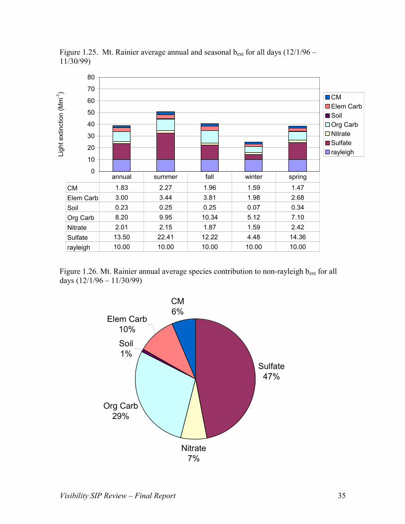
Figure 1.25. Mt. Rainier average annual and seasonal bext for all days (12/1/96 – 11/30/99)

0

10

20

30

40

50

60

70

80

Ligh

t ext

inct

ion

(Mm

-1)




Figure 1.26. Mt. Rainier annual average species contribution to non-rayleigh bext for all days (12/1/96 – 11/30/99)

Sulfate47%

Nitrate7%

Org Carb29%

Soil1%

Elem Carb10%

CM6%


Figure 1.27. Mt. Rainier seasonal average species contribution to non-rayleigh bext for all days (12/1/96 – 11/30/99) Summer Fall

Sulfate40%

Nitrate6%

Org Carb34%

Soil1%

Elem Carb13%

CM6%

Sulfate54%

Nitrate5%

Org Carb25%

Soil1%

Elem Carb9%

CM6%

Winter Spring

Sulfate51%

Nitrate9%

Org Carb25%

Soil1%

Elem Carb9%

CM5%

Sulfate30%

Nitrate11%

Org Carb35%

Soil0%

Elem Carb13%

CM11%


Figure 1.28. Mt. Rainier average annual and seasonal bext for the worst case days (12/1/96 – 11/30/99)

0

10

20

30

40

50

60

70

80

Ligh

t ext

inct

ion

(Mm

-1)




Figure 1.29. Mt. Rainier annual average species contribution to non-rayleigh bext for the worst case days (12/1/96 – 11/30/99)

Sulfate52%

Nitrate7%

Org Carb26%

Soil1%

Elem Carb10%

CM4%


Figure 1.30. Mt. Rainier seasonal average species contribution to non-rayleigh bext for the worst case days (12/1/96 – 11/30/99) Summer Fall

Sulfate48%

Nitrate7%

Org Carb29%

Soil1%

Elem Carb11%

CM4%

24

Sulfate57%

Nitrate5%

Org Carb%

Soil1%

Elem Carb9%

CM4%

Winter Spring 29

Sulfate34%

Nitrate22%

Org Carb%

Soil0%

Elem Carb10%

CM5%

Sulfate53%

Nitrate8%

Org Carb24%

Soil2%

Elem Carb9%

CM4%


Figure 1.31. Alpine Lakes average annual and seasonal bext for the best case days (12/1/96 – 11/30/98)

0

10

20

30

40

50

60

70

80

Ligh

t ext

inct

ion

(Mm

-1)




Figure 1.32. Alpine Lakes annual average species contribution to non-rayleigh bext for the best case days (12/1/96 – 11/30/98)

Sulfate43%

Nitrate12%

Org Carb21%

Soil1%

Elem Carb14%

CM9%


Figure 1.33. Alpine Lakes seasonal average species contribution to non-rayleigh bext for the best case days (12/1/96 – 11/30/98) Summer Fall

Sulfate43%

Nitrate10%

Org Carb28%

Soil1%

Elem Carb12%

CM6%

Sulfate48%

Nitrate6%

Org Carb12%

Soil0%

Elem Carb15%

CM19%

Winter Spring

Sulfate48%

Nitrate11%

Org Carb19%

Soil1%

Elem Carb16%

CM5%

Sulfate41%

Nitrate15%

Org Carb19%

Soil0%

em Carb14%

CM11%

El


Figure 1.34. Alpine Lakes average annual and seasonal bext for all days (12/1/96 – 11/30/98)

0

10

20

30

40

50

60

70

80

Ligh

t ext

inct

ion

(Mm

-1)




Figure 1.35. Alpine Lakes annual average species contribution to non-rayleigh bext for all days (12/1/96 – 11/30/98)

Sulfate44%

Nitrate13%

Org Carb24%

Soil1%

Elem Carb12%

CM6%


Figure 1.36. Alpine Lakes seasonal average species contribution to non-rayleigh bext for all days (12/1/96 – 11/30/98) Summer Fall

Sulfate38%

Nitrate13%

Org Carb30%

Soil1%

Elem Carb14%

CM4%

Sulfate51%

Nitrate8%

Org Carb24%

Soil1%

Elem Carb11%

CM5%

Winter Spring El

Sulfate37%

Nitrate22%

Org Carb20%

Soil0%

em Carb12%

CM9%

Sulfate51%

Nitrate12%

Org Carb18%

Soil2%

Elem Carb11%

CM6%


Figure 1.37 Alpine Lakes average annual and seasonal bext for the worst case days (12/1/96 – 11/30/98)

0

10

20

30

40

50

60

70

80

Ligh

t ext

inct

ion

(Mm

-1)




Figure 1.38. Alpine Lakes annual average species contribution to non-rayleigh bext for the worst case days (12/1/96 – 11/30/98)


Sulfate46%

Nitrate12%

Org Carb25%

Soil2%

Elem Carb11%

CM4%

Figure 1.39. Alpine Lakes seasonal average species contribution to non-rayleigh bext for the worst case days (12/1/96 – 11/30/98) Summer Fall 26

Sulfate51%

Nitrate7%

Org Carb%

Soil1%

Elem Carb11%

CM4%

Sulfate35%

Nitrate14%

Org Carb32%

Soil1%

Elem Carb14%

CM4%

Winter Spring 22

Sulfate31%

Nitrate36%

Org Carb%

Soil0%

Elem Carb8%

CM3%

Sulfate52%

Nitrate10%

Org Carb17%

Soil5%

Elem Carb9%

CM7%


Figure 1.40. Seasonal occurrence of best case and worst case days at Mt. Rainier (12/1/96 – 11/30/99)

0

5

10

15

20

25

30

35

summer fall winter spring

num

ber o

f occ

urre

nces

Best DaysWorst Days

Figure 1.41. Seasonal occurrence of best case and worst case days at Alpine Lakes (12/1/96 – 11/30/98)

0

2

4

6

8

10

12

14

16

summer fall winter spring

num

ber o

f occ

urre

nces

Best DaysWorst Days


1.5 Long-term Mass and Light Extinction Trends at Mt. Rainier One of the main purposes of Visibility SIP review is determining whether progress has been made in remedying existing visibility impairment in mandatory Class I federal areas. Two requirements of the review relate to assessing long-term progress: � Requirement 1. Assess the progress achieved in remedying existing impairment

in any Class I area. This is essentially an assessment and documentation of progress made to date since adoption of the SIP (1986) and its long-term strategy. This assessment is made using visibility aerosol monitoring data from Mt. Rainier only, as it is the only site with enough years of data to meet statistical analysis requirements. Data from the period 12/88 to 11/99 is used for this assessment. Source emission data is also be used to assess progress to date and is covered in section 2 of this report. In the absence of a formal federal definition of “reasonable progress” under the phase I visibility program, we have defined our own for the purpose of this Review. Any statistically significant decrease in light extinction is considered reasonable progress. Additional aerosol trends analysis for other out-of-state mandatory Class I federal areas was also conducted and is presented in section 1.6. Out-of-state sites are Glacier National Park – Montana, and Three Sisters Wilderness – Oregon. These sites are included here for comparison purposes only, and were not used to determine progress for Washington State.

� Requirement 3. Assess any change in visibility since the last report.

This is an assessment of progress made since the last review report and is a subset of the data period covered under requirement 1. Because the period of available data between the last Review Report and this one is only two years, which would not support a statistically valid analysis of trends, we have taken the liberty to use the last five years of data to examine the most recent trends as a surrogate for any changes since the last review. We will continue to do this for future reviews until the regional haze SIP takes effect. Under the regional haze SIP, reviews will be required every five years rather than every three, and changes since the last Review can be supported by statistically valid analysis.

As described in section 1.2, the Theil method was used for determining statistical significance of any trends in the data. Only those trends having a 5% or less cumulative probability of being a random event were considered statistically significant. Although no formal measurable goal or standard exists under the phase I visibility regulation, the regional haze rule explicitly defined a goal of reaching natural visibility conditions by the year 2064. The regional haze rule further defines how to measure progress towards the goal at five-year intervals. Essentially best case days must be preserved (not worsen) and worst case days must improve at a rate equal to a linear glide


path from baseline to natural. The baseline is defined as the average of the five annual averages of the years 2000 – 2004. At the end of this section we will present an example case of tracking progress towards the natural conditions goal using the methods prescribed under the regional haze rule. Trends at Mt. Rainier In this section we examine and present long-term (11 years) and recent (5 years) trends at Mt. Rainier for reconstructed total mass and reconstructed light extinction. For worst case days we will take a closer look at trends in the individual pollutant species that make up total mass and light extinction. Note: In 1996 there was a change made in the monitoring protocol for nitrate. This protocol change may result in a false decreasing nitrate trend when comparing pre- and post-protocol change data. IMPROVE recommended to replacing all nitrate data with an average value based on post-protocol change data. Ecology decided to include a trends analysis with and without the nitrate data included. The following tables present both total and non-nitrate total trends. With the exception of reconstructed total mass on best case days, all categories showed a statistically significant decreasing trend (see tables 1.4 and 1.5). The largest decrease was for worst case days. The slightly positive trend for mass on the best case days was not statistically significant. A closer look at individual pollutant species on the worst case days reveals that each species except for soil showed a statistically significant decreasing trend (see table 1.6). For mass the largest decrease was in coarse mass followed by organic carbon. For light extinction the largest decrease was in organic carbon followed by elemental carbon. There was no trend either way for soil mass or soil light extinction. Table 1.4. Annual trends in total reconstructed mass and light extinction at Mt. Rainier (1988 – 1999). Average mass

change per year (ug/m3)

Statistically significant?

Average light extinction change per year (Mm-1)


Best case days + 0.04 No - 0.30 Yes All days - 0.32 Yes - 1.21 Yes Worst case days - 1.02 Yes - 1.89 Yes Table 1.5 Annual trends in non-nitrate reconstructed mass and light extinction at Mt. Rainier (1988 – 1999) Average non-

NO3 mass change per


Average non-NO3 light extinction



year (ug/m3) change per year (Mm-1)

Best case days + 0.04 No - 0.31 Yes All days - 0.31 Yes - 1.15 Yes Worst case days - 0.99 Yes - 1.58 Yes Table 1.6 Worst case days annual trends in reconstructed mass and light extinction for each pollutant species at Mt. Rainier (1988 – 1999). Average mass

change per year (ug/m3)




Sulfate - 0.04 Yes - 0.25 Yes Nitrate * - 0.03 Yes - 0.31 Yes Organic carbon - 0.15 Yes - 0.60 Yes Soil 0 No trend 0 No trend Elemental Carbon - 0.04 Yes - 0.39 Yes Coarse mass - 0.75 Yes - 0.33 Yes * see note above on nitrate protocol change Figures 1.42 – 1.49 present this data graphically.


Figure 1.42 Mt. Rainier RTM trends for the best case days

0.0

5.0

10.0

15.0

20.0

25.0

89 91 92 93 94 95 96 97 98 99year

ug/m

3


no statistically significant trend

Figure 1.43 Mt. Rainier bext trends for the best case days

0

10

20

30

40

50

60

70

80

90

100

89 91 92 93 94 95 96 97 98 99year

light

ext

inct

ion

(Mm

-1)


statistically significant decreasing trend from 1989 - 1999 (-0.30 Mm-1/year)


Figure 1.44 Mt. Rainier RTM trends for all days

0.0

5.0

10.0

15.0

20.0

25.0

89 91 92 93 94 95 96 97 98 99

year

ug/m

3


statistically significant decreasing trend from 1989 - 1999 (-0.32 ug/m3)

Figure 1.45 Mt. Rainier bext trends for all days

0

10

20

30

40

50

60

70

80

90

100

89 91 92 93 94 95 96 97 98 99

year

light

ext

inct

ion

(Mm

-1)


statistically significant decreasing trend from 1989 - 1999 (-1.21 Mm-1)


Figure 1.46 Mt. Rainier RTM trends for the worst case days

0.0

5.0

10.0

15.0

20.0

25.0

89 91 92 93 94 95 96 97 98 99

year

ug/m

3


statistically significant decreasing trend from 1989 - 1999 (-1.02 ug/m3/year)

Figure 1.47 Mt. Rainier bext trends for the worst case days

0

10

20

30

40

50

60

70

80

90

100

89 91 92 93 94 95 96 97 98 99year

Ligh

t ext

inct

ion

(Mm

-1)


statistically significant decreasing trend from 1989 thru 1999 (-1.89 Mm-1/year)


Figure 1.48 Mt. Rainier RTM pollutant species trends for the worst case days

0.0

2.0

4.0

6.0

8.0

10.0

12.0

89 91 92 93 94 95 96 97 98 99

year

ug/m

3

SulfateNitrateOrg CarbSoilElem CarbCM

Figure 1.49 Mt. Rainier bext pollutant species trends for the worst case days

0

5

10

15

20

25

30

35

40

89 91 92 93 94 95 96 97 98 99

year

light

ext

inct

ion

(Mm

-1)



Change in Visibility since the Last Progress Review Report Because the period of available data between the last Review Report and this one is only two years, which would not support a statistically valid analysis of trends, we have taken the liberty to use the last five years of data to examine the most recent trends as a surrogate for any changes since the last review. Trends at Mt. Rainier for the period 1995 – 1999 were examined and are presented below in table 1.7. Recent trend analysis is limited to worst case light extinction only. Due to data completeness problems at Alpine Lakes, no trend analysis was made for that site. Although average change per year was positive for total light extinction, non-NO3 light extinction, sulfate and organic carbon, no statistically significant trend was detected. Average change per year was negative for nitrate, elemental carbon and coarse mass, but again, no statistically significant trend was detected. There was no trend for soil. Table 1.7 Recent trends in worst case light extinction (1995 – 1999) Average light

extinction change per year (Mm-1)


Total bext +1.21 No Non-NO3 bext +1.50 No Sulfate +1.07 No Nitrate * -0.29 No Organic Carbon +0.72 No Soil 0 No trend Elemental Carbon -0.05 No Coarse Mass -0.24 No * see note above on nitrate protocol change


Tracking Progress under the Regional Haze Rule As mentioned earlier, the regional haze rule has prescribed the establishment of reasonable progress goals for each mandatory Class I federal area and a method for tracking progress towards those goals using light extinction data from IMPROVE monitoring sites. The concept is to establish a current baseline period and determine how much improvement needs to be made in five-year intervals to reach natural visibility levels by the year 2064 (5 year rate of uniform progress). The baseline period is defined as the average of the annual averages for the twenty percent best and worst visibility days for the period 1/1/2000 through 12/31/2004. The goal is to preserve the best case days (not get any worse than the best case baseline) and improve the worst case days to natural conditions over a 64 year period. Although the goal for best case days is to merely maintain current baseline conditions, our analysis below addresses how we are progressing towards estimated natural conditions for best case days. Tracking reasonable progress requires calculation of light extinction in deciviews (dv) rather than inverse magameters (Mm-1). Deciviews are a logarithmic scale of inverse megameters, with rayleigh scatter set to zero. The use of deciviews makes visibility changes in different parts of the country comparable, so that in essence similar changes in deciviews correspond to equally perceptible visibility changes. A one deciview change in visibility is equally perceptible by a viewer whether the current conditions are near pristine or severely degraded and is believed to be more linearly related to barely noticeable changes in visibility near the maximum visual range than other indicators. Deciviews are calculated from inverse megameters by the following equation: dv = 10ln[Bext/10Mm-1] For this analysis we do not have the data from the prescribed 2000 – 2004 baseline period and instead have used the five most recent years of available data as our baseline (1995 – 1999). Estimates of natural conditions were taken from the “Draft Guidance for Estimating Natural Visibility Conditions Under the Regional Haze Rule”, USEPA, September 27, 2001. That guidance recognizes that these estimates may be refined in future years as our understanding of natural conditions improves. Table 1.8 lists the baseline, natural, and rate of progress used for this exercise. Figures 1.53 and 1.54 present this information graphically. Table 1.8 Baseline and natural visibility conditions for Mt. Rainier, rate of progress needed to reach natural conditions in 64 years, and actual rate of progress made. Baseline

Conditions for 1995 – 1999 (dv)

Estimated natural conditions (dv)

Required 5 year rate of uniform progress (dv/5yr)

Actual 5 year rate of progress for 1989 – 1999 (dv/5yr)

Best case days 5.28 2.73 - 0.20 -1.78 Worst case days 19.00 7.85 - 0.87 - 1.91 As can be seen from the tables and graphs the actual rate of progress over the period assessed is significantly better than required. The rate of progress on the best case days is


more than eight times better than required to reach natural conditions in 64 years. The rate of progress on the worst case days is more than twice that required. However, no predictive modeling was performed to determine if this rate of change will continue in future years. Figure 1.53 Tracking progress under the regional haze rule for best case days at Mt. Rainier

0.0

5.0

10.0

15.0

20.0

25.0

30.0

year

Haz

e In

dex

(dv)

Deciview 6.87 7.15 7.54 7.62 6.13 4.86 5.85 5.40 4.83 5.451989 1991 1992 1993 1994 1995 1996 1997 1998 1999

'89 - '94 avg = 7.06 Dv '95 - '99 avg = 5.28 Dv

Actual 5yr avg change = -1.78 DvRequired 5yr urp = -0.20 Dv

actual rate of progress is better than urp

using '95 - '89 as baseline and natural best case = 2.73 Dv

[(5.28-2.73)/64]5=0.20

Figure 1.54 Tracking progress under the regional haze rule for worst case days at Mt. Rainier

0.0

5.0

10.0

15.0

20.0

25.0

30.0

year

Haz

e In

dex

(dv)

Deciview 21.86 21.29 20.74 20.26 20.39 18.61 18.73 18.60 19.73 19.321989 1991 1992 1993 1994 1995 1996 1997 1998 1999

'89 - '94 avg = 20.91 Dv '95 - '99 avg = 19.00 Dv

Actual 5yr avg change = -1.91 DvRequired 5yr urp = -0.87

actual rate of progress is better than urp

using '95 - '99 as base line and natural worst case = 7.85 Dv[(19.00-7.85)/64]5=0.87 Dv


1.6 Light Extinction Conditions and Trends at Other Mandatory Class I Federal Areas in the Pacific Northwest For the purpose of comparing visibility at Washington State mandatory Class I federal areas, visibility was assessed at two other nearby but out of state mandatory Class I federal areas of the Pacific Northwest. Methods used for this analysis were the same as applied to the sites described in previous sections. Visibility Conditions at other Mandatory Class I Federal Areas Table 1.9 lists the sites and various visibility conditions. Light extinction levels are somewhat similar to Washington’s mandatory Class I federal areas, although Three Sisters Wilderness has a somewhat higher best case average than the other sites. Mt. Rainier has the highest worst case light extinction. The sites are dissimilar in the relative contribution to worst case light extinction by individual pollutant species. The two Washington sites are clearly dominated by sulfate followed by organic carbon, whereas Glacier National Park is dominated by organic carbon followed by sulfate. Three Sisters Wilderness is interesting in that sulfate, organic carbon and nitrate contribute nearly equal to worst case light extinction. Table 1.9 Visibility conditions at other Pacific Northwest Class I monitoring sites compared to Mt. Rainier and Alpine Lakes for the period 12/1/96 – 11/30/99 Best case

average (Mm-1)

All days average (Mm-1) *

Worst case average (Mm-1)

Pollutant species contributing the most to worst case bext

Glacier National Park - MT

22.02 40.11 (natural = 16.58)

66.52 OC (35%) SO4 (26%) CM (18%)

Three Sisters Wilderness - OR

29.89 42.52 (natural = 16.79)

64.58 SO4 (29%) OC (28%) NO3 (26%)

Mt. Rainier National Park - WA

17.04 38.77 (natural = 16.97)

69.25 SO4 (52%) OC (26%) EC (10%)

Alpine Lakes Wilderness - WA**

18.45 36.23 (natural = 16.79)

61.48 SO4 (46%) OC (25%) NO3 (12%)

* Estimates for average natural levels taken from “Draft Guidance for Estimating Natural Visibility Conditions Under the Regional Haze Rule”, USEPA, September 27, 2001 ** Alpine Lakes period of assessment is 12/96 – 11/98 Light Extinction Trends at Other Mandatory Class I Federal Areas Table 1.10 presents the average change in light extinction for Glacier National Park and Three Sister Wilderness. There is a statistically significant increasing trend at Three


Sisters Wilderness for total light extinction and for light extinction due to organic carbon. There is a slight decreasing trend in nitrate that is statistically significant. There were no statistically significant trends at Glacier National Park. Trends are also presented graphically in figures 1.55 – 1.58. Table 1.10 Annual trends in worst case light extinction at Glacier National Park and Three Sisters Wilderness.

Glacier National Park (1989 – 1999)

Three Sisters Wilderness (1995 – 1999)





Total bext + 0.68 No + 1.17 Yes

Non-NO3 bext +0.94 No +1.57 Yes

Sulfate - 0.10 No - 0.06 No

Nitrate - 0.26 No - 0.40 Yes

Organic Carbon

- 0.10 No + 1.32 Yes

Soil + 0.16 No + 0.01 No

Elemental Carbon

- 0.18 No + 0.11 No

Coarse mass + 1.16 No +0.19 No


Figure 1.55 Trends in annual reconstructed light extinction for the worst case days at Glacier National Park

0

10

20

30

40

50

60

70

80

90

100

89 90 91 92 93 94 95 96 97 98 99year

light

ext

inct

ion

(Mm

-1) CM

Elem CarbSoilOrg CarbNitrateSulfaterayleigh

no statistically significant trend

Figure 1.56 Trends in individual pollutant species for the worst case days at Glacier National Park

0

5

10

15

20

25

30

89 90 91 92 93 94 95 96 97 98 99year

light

ext

inct

ion

(Mm

-1)



Figure 1.57 Trends in annual reconstructed light extinction for the worst case days at Three Sisters Wilderness

0

10

20

30

40

50

60

70

80

90

100

95 96 97 98 99year

light

ext

inct

ion

(Mm

-1) CM

Elem CarbSoilOrg CarbNitrateSulfaterayleigh

statistically significant increasing trend from 1995 thru 1999 (+1.17 Mm-1/yr)

Figure 1.58 Trends in individual pollutant species for the worst case days at Three Sisters Wilderness

0

2

4

6

8

10

12

14

16

18

20

95 96 97 98 99year

light

ext

inct

ion

(Mm

-1)



1.7 Conclusions The following is a brief summary of conclusions with respect to aerosol mass and light extinction analysis conducted for this review report. � In most cases at the two aerosol monitoring sites analyzed (Mt. Rainier National Park

and Alpine Lakes Wilderness) non-speciated coarse mass dominates the total mass (PM10) while organic carbon dominates the fine mass (PM2.5), followed by sulfate.

� Worst case total mass (average of the worst 20% days) is 12.01 ug/m3 at Mt. Rainier and 11.77 ug/m3 at Alpine Lakes.

� Worst case fine mass is 8.21 ug/m3 for Mt. Rainier and 7.88 ug/m3 at Alpine Lakes. � In all cases at both sites reconstructed light extinction is dominated by sulfate

followed by organic carbon. � At Mt. Rainier, reconstructed light extinction levels range from 17.04 Mm-1 for the

best case days (natural conditions are estimated at 13.14 Mm-1) to 69.25 Mm-1 for the worst case days.

� At Alpine Lakes reconstructed light extinction levels range from 18.45 Mm-1 for the best case days (natural conditions are estimated at 13.00 Mm-1) to 61.48 Mm-1 for the worst case days.

� Most of the worst case days occur in summer and most of the best case days occur in winter at both sites.

� Trends in reconstructed light extinction for the best case, average and worst case days showed a statistically significant decreasing trend (improving visibility) at Mt. Rainier for the period 1989 to 1999. There were not enough years meeting minimum data completeness to determine a trend at Alpine Lakes.

� However, closer examination of recent trends (1995 - 1999) indicates that there is no statistically significant trend in either direction at Mt. Rainier for the more recent period.

� A closer look at individual pollutant species contributing to light extinction indicates that all species except soil showed a statistically significant decreasing trend at Mt. Rainier.

� Using the method prescribed in the regional haze rule, the trend in visibility at Mt. Rainier is estimated to be improving for the period 1989 - 1999 at a rate that would lead to natural conditions by the year 2064 if that rate were to continue. However, actual visibility levels after the year 1999 cannot be predicted.

� Two other Class I area aerosol monitoring sites outside of Washington State were analyzed. Light extinction levels were similar to those in Washington, although individual pollutant species contribution to light extinction was different from that seen at the Washington sites. Organic carbon dominated light extinction at Glacier National Park and at Three Sisters Wilderness sulfate, organic carbon and nitrate contributed to light extinction nearly equally.


References for Section 1.0 UC Davis, “IMPROVE Particulate Monitoring Network Procedures for Site Selection”, Crocker Nuclear Laboratory, University of California, Davis, CA, February 24, 1999 USEPA, “Draft Guidance for Tracking Progress Under the Regional Haze Rule”, Office of Air Quality Planning and Standards, Research Triangle Park, NC, September 27, 2001 Malm et al, “Spatial and Seasonal Patterns and Temporal Variability of Haze and its Constituents in the United States: Report III”, CIRA, CSU, May 2000. USEPA, “Visibility in Mandatory Federal Class I Areas (1994-1998): A Report to Congress", Office of Air Quality Planning and Standards, Research Triangle Park, NC, November 2001 USEPA, “Draft Guidance for Estimating Natural Visibility Conditions Under the Regional Haze Rule”, Office of Air Quality Planning and Standards, Research Triangle Park, NC, September 27, 2001


2.0 REVIEW OF EMISSIONS DATA Air quality control programs, both non-visibility and visibility-specific programs, have been responsible for reducing emissions or preventing the increase of emissions which affect visibility. An analysis of emissions data was made to help address Visibility SIP review requirements, particularly requirements: 1) progress achieved in remedying existing visibility impairment in any Class I area, 2) ability of the long-term strategy to prevent future visibility impairment in any Class I area, and 4) need for additional measures to assure reasonable further progress toward remedying existing and preventing future impairment. 2.1 Scope of the Emissions Inventory In 1999 a statewide emissions inventory was constructed to support a review of the Visibility SIP. Major sources of the following visibility impairing pollutants were addressed: primary particulate matter (PM10 and PM2.5), sulfur dioxide (SO2), nitrogen oxides (NOx), volatile organic compounds (VOC), and ammonia (NH3). Estimates of emissions were made by county and month for the years 1985, 1996 and 2010. 1985 was the base year of the original Visibility SIP; 1996 was the year of the most current emissions inventory, and 2010 was a future projection. For this SIP review, 1985 and 1996 were retained as the original base year and the year of the most current emissions inventory, respectively. The projection year was changed to 2018 in an effort to align the SIP review effort with requirements of the upcoming regional haze SIP. Several source categories in the emissions inventory were updated and additional source categories were added (please see Appendix B for a detailed list of updates and added categories). A more comprehensive update of the emissions inventory will be done for the upcoming regional haze SIP. Sources and pollutants included in the inventory are shown in Table 2.1. New sources added for this review, and sources which were updated are shown in italics.


Table 2.1: Sources and Pollutants Inventoried Source Category Pollutants Onroad Mobile Sources SO2, NOx, PM10/PM2.5, VOC, CO, NH3 Road Dust, Paved and Unpaved PM10/PM2.5 Nonroad Mobile Sources (nonroad equipment and vehicles, aircraft, marine vessels)

SO2, NOx, PM10/PM2.5, VOC, CO, NH3

Nonroad Mobile Sources (locomotives) SO2, NOx, PM10/PM2.5, VOC, CO Prescribed Burning SO2, NOx, PM10/PM2.5, VOC, CO Agricultural Field Burning SO2, NOx, PM10/PM2.5, VOC, CO Solvent Usage (architectural coatings and consumer/commercial solvents)

VOC

Point Sources SO2, NOx, PM10/PM2.5, VOC, CO Wood stoves/Fireplaces SO2, NOx, PM10/PM2.5, VOC, CO Agricultural Dust (tilling and windblown) PM10/PM2.5 Livestock NH3 Fertilizer Application NH3 Biogenics VOC, NOx Soils NH3

2.2 Emissions Inventory Discussion A discussion of findings and trends for each major source category of emissions follows. Figure 2.5 through Figure 2.12 and Table 2.4 through Table 2.6 show the emissions and trends. Short discussions on spatial and temporal distribution of emissions are also included. More detailed documentation on the inventory may be found in Appendix B. 2.2.1 Phase I Sources Phase I of visibility regulations required states to develop visibility protection SIPs that addressed visibility impairment that was easily attributable to certain types of sources that contributed to this impairment (mostly major stationary sources and prescribed burning). Washington’s approved Phase I Visibility SIP developed long-term strategies that addressed emissions from major stationary sources and prescribed burning. Therefore, it is important to examine this subset of all visibility impairing emission sources to determine if reasonable progress has been made and will continue to be made under the Phase I Visibility SIP. Point Sources Point sources contribute to all visibility-impairing pollutants and are major contributors to the particulate, NOx, and particularly the SO2 inventories. Between 1985 and 1996, significant decreases were observed in all pollutants except NOx, which showed a modest decrease. Much of the decrease in SO2 emissions can be attributed to the closure of


Asarco, and to a lesser extent, by the cessation of the rotary cement kiln operations of Columbia Cement (now Tilbury Cement). Other differences are more difficult to assess. A word of caution is appropriate concerning the comparability of 1985 and 1996 emissions estimates for individual sources. Differences may reflect decreased operation or improvements in controlling emissions, or changes in calculation method or updated emission factors. During the ten-year interval, air quality issues put increasing emphasis on emissions estimations. Only a careful, source-specific analysis can distinguish reasons for differences between the two inventory years. Between 1996 and 2018, emissions of SO2 show a marked decrease, while particulate emissions show a modest increase. Other pollutants show only minor changes. The primary source of the SO2 decrease is the Centralia Power Plant, which is now meeting emissions limits of 10,000 tons per year of SO2 and 16,000 tons per year of NOx as part of a regulatory order establishing Reasonably Available Control Technology (RACT). These emission limits represent an 87% (68,000 tpy) reduction in SO2 and a 14% (2,600 tpy) reduction in NOx from 1996 levels. This is a major reduction in emissions. Other changes in emissions between 1996 and 2018 can be attributed to expected closures of several major industrial facilities, and current and projected new source permitting, primarily in the area of gas turbines for power generation and gas compressors. It is estimated that power needs may increase by an average of 120 megawatts per year from 2002 to 2018. Based on current permits, this will result in fairly small emissions increases (increases are: PM = 43 tpy, NOx = 30 tpy, SO2 = 14 tpy, VOC = 32 tpy and CO = 19 tpy). Prescribed Burning Prescribed burning is a fairly significant source of particulate matter. As a result of the 1991 Washington Clean Air Act, a two-phase emissions reduction goal was set for prescribed burning. The first target was a 20% reduction by 1994; the second target was a 50% reduction by 2000. Both targets were met. Large decreases in emissions were observed between 1985 and 1996. Between 1996 and 2018, emissions are predicted to increase slightly above the 50% reduction target level. The increase is due to future plans by the US Forest Service to increase burning in eastern Washington for forest health. Compliance with the Endangered Species Act has resulted in less tree cutting, and virtually no clear cutting on Forest Service land, resulting in decreased burning in the past several years. The decrease in burning has led to buildups of material that may pose a threat to forest health due to increased wildfire and disease risk. Plans to alleviate the risk by increasing prescribed burning are being discussed. Increased prescribed burning will be dependent on public reaction, funding, and weather conditions. No increase is projected for western Washington or on state or private lands.


2.2.2 Other Emission Sources (Regional Haze Sources) The focus of the phase I Visibility SIP is on point sources and prescribed burning; however, it is recognized that other sources affect visibility. To better understand these sources and to prepare for upcoming development of a regional haze SIP, other sources of visibility-impairing emissions were assessed. Agricultural Field Burning Agricultural field burning is a fairly significant source of particulate matter. Estimates of emissions from agricultural field burning were not available for 1985, and so were assumed the same as 1996. Estimates focused on current and future conditions. In a 1999 agreement among Ecology, the state Department of Agriculture and the Washington Association of Wheat Growers, wheat growers committed to reduce field burning by at least half by 2006. The anticipated reductions are reflected in the 2018 estimates. Residential Wood stoves and Fireplaces Residential wood combustion is the largest source of particulate matter from non-dust related sources. It also contributes significantly to the VOC inventory. Wood stove emissions show an increase from 1985 through 2018, due to increases in population and wood burning habits. Several factors work to lessen the effect of increased wood burning activity. Advances in stove efficiency and emissions control technology have in part offset emissions increases. While wood stove curtailment programs are designed to dramatically decrease activity during periods of air stagnation for health reasons they also lessen effects of visibility impairment due to wood combustion. In addition, future fuel costs and wood availability will affect emissions. Onroad Mobile Sources Onroad mobile sources contribute to all visibility-impairing pollutants and are major contributors to the NOx, VOC, CO and NH3 inventories. Between 1985 and 1996, the benefits of a series of federal and state control programs enacted in the 1970s, 80s and early 90s were seen. NOx, VOC and CO emissions all decreased. Much larger decreases in all of the criteria pollutants are predicted between 1996 and 2018 due to three new federal control programs: Tier 2 Motor Vehicle Emissions Standards, the National Low Sulfur Gasoline Program, and the 2007 Diesel Rule addressing heavy duty engine standards and diesel fuel sulfur content. Attainment and maintenance planning areas have emissions budgets (caps) which also serve to limit or prevent growth in mobile source emissions. With the projected decreases onroad is still an important source, but no longer the dominant source of NOx and anthropogenic VOC in the overall inventory. Increases in NH3 are projected from 1985 through 2018. Nonroad Mobile Sources Nonroad mobile sources are all mobile sources not generally operated on public roadways (e.g. ships, locomotives, aircraft, construction equipment, lawnmowers). Nonroad sources are significant contributors to all visibility-impairing pollutants except NH3. Emissions from nonroad sources increased between 1985 and 1996. Three tiers of federal emissions standards are being phased in from 1996 through 2008. The standards


address NOx, VOC and particulates. A significant decrease in VOC is projected between 1996 and 2018. A more modest decrease is projected for NOx, and there is virtually no change in particulates. Because nonroad controls have not been as stringent as onroad controls, nonroad sources have become an increasingly large portion of the overall mobile source inventory. Future federal control program proposals may include lowering diesel fuel sulfur content from 3000 ppm to 15 ppm. This would result in decreases in particulate, NOx and SO2 emissions. Solvent Usage Use of solvents produces VOC emissions. Solvent sources inventoried included only architectural surface coating and commercial/consumer product use. Future inventories may expand this inventory to include other solvent sources such as solvent cleaning and industrial surface coating. The sources inventoried for this SIP review did not contribute a large amount of VOC. Between 1985 and 1996 emissions increased due to increased activity level resulting from increased population. Maximum achievable control technology (MACT) standards were promulgated for both architectural coatings and commercial/consumer products in 1998. Reductions of 20% from 1990 levels were expected. The MACT standards resulted in offsetting most of the emissions increase expected between 1996 and 2018. Agricultural Ammonia Sources Agricultural ammonia sources include fertilizer application and livestock waste operations. Agricultural sources are the largest sources of NH3 in the inventory. Little information was readily available on either past or future activity levels. So the 1996 emissions levels were used for both the 1985 and 2018 inventories. Fugitive Dust Sources Fugitive dust sources include dust from paved and unpaved roads, agricultural tilling, and windblown dust from agricultural fields. With current inventory methods, dust sources completely dominate the PM10 inventory. Yet coarse mass accounts for very little of the light extinction measured at Class I monitoring sites. Though not so dominant, dust emissions are also very significant contributors to the PM2.5 inventory. The generation of dust emissions and their effect on visibility impairment are not easily inventoried. Dust emissions are highly variable, and depend on a variety of factors including meteorology, surface silt loading, and vegetative cover. More information is needed on transport and deposition characteristics of dust as well. Better characterization of dust emissions is a topic of ongoing research within the EPA, Western Regional Air Partnership (WRAP) and other organizations. Natural Sources


Natural sources include VOC, NOx and NH3 emissions from vegetation (biogenics) and soils. No changes were estimated from 1985 through 2018. The inventory is based on 1996 emissions calculations. 2.2.3 Spatial Distribution The mixture and proximity of sources to individual mandatory Class I federal areas affect visibility impairment. Source impacts on visibility impairment are addressed through modeling. Models typically require information on source locations, as well as temporal and chemical characteristics of emissions. Figure 2.1 and Figure 2.2 show general differences in emissions and sources in eastern and western Washington. Note that in Figure 2.2 CO emissions are divided by 10 so that they could be displayed on the graph with other pollutants.


Figure 2.1: Eastern and western Washington 1996 emissions: PM and NH3

0

50000

100000

150000

200000

250000

PM10 dust PM2.5 dust PM10 other PM2.5 other NH3

tons

/yea

r

east west

Figure2.2: Eastern and western Washington 1996 emissions: NOx, SO2, VOC, CO

0

100000

200000

300000

400000

500000

600000

700000

NOx SO2 VOC CO / 10

tons

/yea

r

east west


2.2.4 Temporal Distribution Some emissions sources operate on a fairly constant temporal basis (e.g. most industrial sources); others can vary according to season (e.g. wood stove use, biogenics), and still others may vary widely within a season on a day-to-day basis (prescribed and agricultural field burning). Seasonal, daily and hourly variations affect the impact emissions sources have on visibility impairment. Examples of seasonal variation are shown in Figure 2.3 and Figure 2.4. Figure 2.3: Seasonal variation in statewide PM2.5 emissions, 1996

PM2.5 emissions, fall

All Mobile

Outdoor Burning

Point Sources

Wood Stoves

PM2.5 emissions, spring

All Mobile

Outdoor Burning

Wood Stoves

Point Sources

PM2.5 emissions, summer

All Mobile

Outdoor Burning

Point Sources

Wood Stoves

PM2.5 emissions, winter

All MobileOutdoor Burning

Wood Stoves

Point Sources

Figure 2.4: Seasonal variation in statewide VOC emissions, 1996

VOC emissions, summer

Natural Sources

Onroad

Nonroad

Other

VOC emissions, w inter

Natural Sources

Nonroad

OtherOnroad

Wood Stoves

2.3 Conclusions


The analysis of emissions data is one tool to address Visibility SIP requirements of assessing: 1) progress achieved in remedying visibility impairment, 2) ability of the long-term strategy to prevent future impairment, and 3) the need for additional measures to assure continued progress in remedying current and preventing future impairment. The focus of the phase I Visibility SIP is on point sources and prescribed burning. This SIP review focuses on these sources, but also looks at a more comprehensive set of emissions sources. Conclusions are presented for both the Phase I sources, and for all sources inventoried for this review. The conclusions are based strictly on emissions inventory. As more regional air quality modeling is performed, better assessments of the effects of emissions on visibility impairment in mandatory Class I federal areas can be made. 2.3.1 Phase I Sources Between 1985 and 1996 the combined emissions from point sources and prescribed burning for each pollutant decreased (see Figure 2.13). During the timeframe between 1996 and 2018, PM, VOC and CO are expected to increase, while NOx and SO2 emissions are expected to decrease. Looking at the longer timeframe between 1985 and 2018, all pollutant emissions are projected to decrease. Point source closures, new emission limits for the Centralia Power Plant, and decreased prescribed burning activity all contribute to overall phase I emissions decreases. It is concluded that progress has been made and will continue to be made in reducing emissions from sources that the phase I control strategies target. Emissions from the projected increase in prescribed burning activity and anticipated new point sources will not overtake emission decreases made to Phase I sources in the past seventeen years. Table 2.2 Percent Change in Emissions, Phase I Sources timeframe PM10 PM2.5 SO2 NOx VOC CO 1985-1996 -54 -55 -14 -7 -38 -521996-2018 24 31 -59 -4 6 31985-2018 -43 -41 -65 -11 -35 -51 2.3.2 All Emissions Sources (Regional Haze Sources) Between 1985 and 1996 the combined emissions from all sources for each pollutant except PM and NH3 decreased. From 1996 to 2018 and from 1985 to 2018, all pollutant emissions are predicted to decrease except NH3 and PM10 (see Figure 2.14). If dust sources of PM are removed, PM10 also decreases. While the emissions of most of the visibility-impairing pollutants decrease from the present into the future, some sources show increasing trends for at least one pollutant. PM2.5 emissions from nonroad mobile, point sources, prescribed burning, wood stoves and road dust all have increasing trends in the future. SO2 and CO emissions are


predicted to increase from nonroad sources. VOC emissions from wood stoves and NH3 emissions from onroad sources are predicted to increase. All of these sources will be addressed further through the upcoming regional haze SIP. Table 2.3 Percent Change in Emissions, All Emissions Sources (Regional Haze sources)

timeframe PM10 PM2.5 PM10

(w/o dust)PM2.5

(w/o dust) SO2 NOx VOC CO NH3 1985-1996 -2 -8 -17 -15 -10 -5 -1 -9 61996-2018 4 1 2 0 -45 -39 -9 -28 101985-2018 2 -7 -16 -14 -51 -42 -10 -35 16


Table 2.4: 1985 Emissions Estimates in Tons Major Category PM10 PM25 SO2 NOx VOC CO NH3

Agricultural Field Burning 12,647 12,072 nd nd 7,473 73,583 ndAgricultural Fugitive Dust 90,304 18,332 0 0 0 0 0Area Source Solvents 0 0 0 0 23,851 0 0Fertilizer Application 0 0 0 0 0 0 11,548Livestock Wastes 0 0 0 0 0 0 12,088Natural Sources 0 0 0 21,447 636,008 0 1,350Nonroad Mobile Sources 11,956 11,024 23,719 148,506 80,579 523,384 360Onroad Mobile Sources 5,993 4,665 8,869 240,638 238,329 2,690,347 2,317Point Sources 24,787 18,370 139,716 57,290 30,514 343,749 ndPrescribed Burning 15,636 14,335 170 4,528 8,232 126,785 ndRoad Dust 168,606 24,461 0 0 0 0 0Woodstoves and Fireplaces 28,030 27,350 360 2,494 69,838 210,364 nd total all sources 357,959 130,609 172,833 474,902 1,094,824 3,968,212 27,663 total Phase I sources 40,423 32,705 139,886 61,818 38,746 470,534 ndnd = no data Table 2.5: 1996 Emissions Estimates in Tons Major Category PM10 PM25 SO2 NOx VOC CO NH3

Agricultural Field Burning 12,647 12,072 nd nd 7,473 73,583 ndAgricultural Fugitive Dust 90,304 18,332 0 0 0 0 0Area Source Solvents 0 0 0 0 31,031 0 0Fertilizer Application 0 0 0 0 0 0 11,548Livestock Wastes 0 0 0 0 0 0 12,744Natural Sources 0 0 0 21,447 636,008 0 1,350Nonroad Mobile Sources 12,781 11,784 28,268 159,811 115,181 726,604 421Onroad Mobile Sources 6,298 5,553 5,141 208,291 193,243 2,347,829 3,329Point Sources 12,587 9,379 120,811 55,624 20,711 174,414 ndPrescribed Burning 5,957 5,487 66 1,760 3,171 49,293 ndRoad Dust 178,325 26,244 0 0 0 0 0Woodstoves and Fireplaces 31,603 30,739 460 2,936 76,618 234,986 nd total all sources 350,502 119,590 154,746 449,869 1,083,436 3,606,709 29,392 total Phase I sources 18,544 14,866 120,877 57,384 23,882 223,707 ndnd = no data Table 2.6: 2018 Emissions Estimates in Tons Major Category PM10 PM25 SO2 NOx VOC CO NH3

Agricultural Field Burning 6,324 6,036 nd nd 3,737 36,791 ndAgricultural Fugitive Dust 90,304 18,332 0 0 0 0 0Area Source Solvents 0 0 0 0 33,402 0 0Fertilizer Application 0 0 0 0 0 0 11,548Livestock Wastes 0 0 0 0 0 0 12,744Natural Sources 0 0 0 21,447 636,008 0 1,350Nonroad Mobile Sources 12,813 11,805 33,672 138,648 68,154 949,093 599Onroad Mobile Sources 2,100 2,002 663 52,462 64,857 1,071,566 5,946Point Sources 13,876 11,160 49,220 52,508 20,881 156,168 ndPrescribed Burning 9,082 8,282 98 2,614 4,410 73,191 ndRoad Dust 190,373 27,831 0 0 0 0 0Woodstoves and Fireplaces 39,093 35,807 751 5,688 156,438 299,584 nd total all sources 363,964 121,256 84,404 273,367 987,885 2,586,394 32,187 total Phase I sources 22,957 19,442 49,318 55,122 25,291 229,359 ndnd = no data


Figure 2.5: Trends in PM10 emissions by source category (excludes dust sources)

0

5000

10000

15000

20000

25000

30000

35000

40000

45000

Agricultural FieldBurning

Nonroad MobileSources

Onroad MobileSources

Point Sources PrescribedBurning

Woodstovesand Fireplaces

tons

/yea

r

1985 1996 2018

Figure 2.6: Trends in PM2.5 emissions by source category (excludes dust sources)

0

5000

10000

15000

20000

25000

30000

35000

40000

AgriculturalField Burning





tons

/yea

r

1985 1996 2018


Figure 2.7: Trends in dust emissions by source category, PM10 and PM2.5

0

20000

40000

60000

80000

100000

120000

140000

160000

180000

200000

PM10: AgriculturalFugitive Dust

PM10: Road Dust PM2.5: AgriculturalFugitive Dust

PM2.5: Road Dust

tons

/yea

r

1985 1996 2018

Figure 2.8: Trends in SO2 emissions by source category

0

20000

40000

60000

80000

100000

120000

140000

160000



Other Point Sources

tons

/yea

r

1985 1996 2018


Figure 2.9: Trends in NOx emissions by source category

0

50000

100000

150000

200000

250000

300000

Natural Sources Nonroad MobileSources


Other Point Sources

tons

/yea

r

1985 1996 2018

Figure 2.10: Trends in VOC emissions by source category

0

100000

200000

300000

400000

500000

600000

700000

NaturalSources

Area SourceSolvents

NonroadMobile

Sources


Other Point Sources Woodstovesand

Fireplaces

tons

/yea

r

1985 1996 2018


Figure 2.11: Trends in NH3 emissions by source category

0

2000

4000

6000

8000

10000

12000

14000

FertilizerApplication

Livestock Wastes Natural Sources Nonroad MobileSources


tons

/yea

r

1985 1996 2018

Figure 2.12: Trends in CO emissions by source category

0

500000

1000000

1500000

2000000

2500000

3000000

AgriculturalField Burning





tons

/yea

r

1985 1996 2018


Figure 2.13: Trends in phase I target source emissions (excluding CO)

0

50000

100000

150000

200000

250000

300000

1985 1996 2018

tons

/yea

r

PM (coarse)PM2.5 SO2 NOx VOC

Figure 2.14: Trends in the total of all visibility impairing emissions (excluding CO)

0

500000

1000000

1500000

2000000

2500000

1985 1996 2018

tons

/yea

r

PM (coarse)PM2.5 NH3 SO2 NOx VOC


2.4 County and Emission Zone Trends Purpose Although it is useful to understand emission trends on a broad geographical scale as presented in the preceding sections, it is also useful to understand trends on scales more representative of individual or geographical groups of mandatory Class I federal areas. For this purpose, we took a closer look at emission trends at the county level and also grouped counties into geographical emission zones in which it may be reasonable to anticipate them to affect mandatory Class I federal areas in the zone. The concept is that if any particular counties or groups of counties in an emission zone show increasing emissions in the future, we would take a closer look at the types of emissions, types of sources, and relative location with respect to mandatory Class I federal areas to see if we can reasonably anticipate whether these emissions will affect visibility. This may have implications on how we would manage emissions in these counties or zones to prevent future impairment of visibility in the affected mandatory Class I federal area. For this assessment we limited our scrutiny to emission projections from 1996 to 2018. We included all visibility impairing emissions from the inventory, but did not include carbon monoxide as it does not affect visibility. We included all source categories in the inventory, not just phase I types. We looked at each of the 39 counties in Washington State. We further grouped them into 3 geographical zones consisting of counties within 100 km of the centroid of: 1) mandatory Class I federal areas in the northern Cascades, 2) mandatory Class I federal areas in the southern Cascades and, 3) the one Class I area on the Olympic Peninsula (Olympic National Park). Counties that had at least half their area within 100 km of the centroid of any Class I area in each of these zones were included in the respective zone. Therefore, several counties ended up in more then one emission zone. In addition, Snohomish, King, Pierce and Thurston counties were included in the Olympic Peninsula zone because high-density emission areas in those counties were within 100 km of Olympic National Park. Table 2.7 lists the counties and mandatory Class I federal areas in each zone.


Table 2.7 Counties and mandatory Class I federal areas in the emission zones.

Northern Cascade Zone Southern Cascade Zone Olympic Peninsula Zone Mandatory Class I federal areas

Counties Mandatory Class I federal areas

Counties Mandatory Class I federal areas

Counties

-North Cascades NP -Pasayten W -Glacier Peak W -Alpine Lakes W

-Whatcom -Skagit -Snohomish -King -Pierce -Kittitas -Chelan -Okanogan

-Mt. Rainier NP -Goat Rocks W -Mt. Adams W

-King -Pierce -Thurston -Lewis -Cowlitz -Skamania -Klickitat -Yakima -Kittitas

-Olympic NP -San Juan -Island -Kitsap -Mason -Grays Harbor -Jefferson -Clallam -Snohomish -King -Pierce -Thurston

Projected Trends for Counties and Emission Zones Projected emission changes between 1996 and 2018 show a decrease in visibility impairing emissions in every county except Pend Oreille which showed a slight increase of 0.6%. The decrease in emissions ranged from 1.7% in Skamania County to 51.6% in Lewis County (mostly attributable to controls being installed on the coal-fired power plant near Centralia). Seventeen counties showed a decrease ranging from 1.7 to 10 percent, 15 counties showed a decrease ranging from 10 to 20 percent and six counties showed a decrease greater than 20 percent. The emission zones showed significant decreases in visibility impairing emissions. The northern Cascades zone showed a 15.9% decrease, the southern Cascades zone showed a 23.2% decrease and the Olympic Peninsula zone showed a 19.0% decrease in emissions. Table 2.8 lists the emission changes for each county and emission zone.


Table 2.8 Projected emission changes for counties and emission zones for the period 1996 to 2018. +1 to -10% change -10 to -20% change Greater than -20%

change Emission Zone change

county Percent change

county Percent change

County Percent change

Zone Percent change

Adams -10.0 Kitsap -18.1 Lewis -51.6 N. Cascades -15.9

Spokane -9.8 Snohomish -17.6 Clark -25.4 S. Cascades -23.2

Asotin -9.5 Clallam -16.9 Island -24.2 Olym Penins -19.0

Wahkiakum -9.3 Columbia -16.7 King -22.4 Lincoln -9.0 Benton -15.1 Cowlitz -21.7 Yakima -8.9 GraysHarbor -14.7 Pierce -20.4 Grant -8.2 Thurston -13.7 Franklin -8.2 Whitman -13.6 Klickitat -6.5 Mason -13.1 Jefferson -6.5 Pacific -12.8 Chelan -6.5 Douglas -11.4 Garfield -3.2 Whatcom -11.4 Stevens -3.0 Walla Walla -11.4 San Juan -2.7 Kittitas -11.2 Ferry -2.2 Skagit -11.0 Okanogan -1.9 Skamania -1.7 Pend Oreille +0.6 Comparing Projected Emission Reductions with Light Extinction Reductions Needed to Reach Natural Conditions by the Year 2064 Our analysis of tracking progress under the Regional Haze Rule presented in section 1.5 indicates that a decrease in light extinction of 0.174 dv/yr (0.870 dv over 5 years) is needed to stay on the linear glide path to natural conditions by the year 2064. This equates to a light extinction level of 15.87 dv by the year 2018 or a 16% reduction in light extinction between 2000 and 2018. Using this same period (2000 to 2018) for the projected emission trend (assuming a straight line from 1996 to 2018), the amount of emission reductions for the period 2000 to 2018 for the emission zone affecting Mt. Rainier is 19.0%. The projected amount of reduction in emissions for the southern Cascade emission zone is greater than the amount of light extinction reduction required for that period to stay on the linear glide path to natural conditions by 2064 for Mt. Rainier, if that rate were to continue. However, actual emission levels after the year 2018 were not estimated, and it is unknown if this rate will continue without additional control strategies. An important caveat about the above analysis is an assumption is made that there is a 1:1 relationship between emissions reduced and light extinction reduced (visibility improved). This is a conservative assumption because under normal Pacific Northwest


conditions pollutant species cause more light extinction then their unadjusted dry masses would allow. Therefore, reducing emissions should actually cause more reduction in light extinction then a 1:1 ratio. Nonetheless, it is important to note that air quality levels resulting from the projected emission reductions were not modeled.


3.0 TRAJECTORY ANALYSIS The Penn State - NCAR mesoscale model MM5 has been used to produce forecasts of meteorological variables for a domain covering most of the Pacific Northwest twice each day for the past several years, first at a 27 km grid spacing and, more recently, as a triply-nested grid of 36, 12, and 4 km spacing. Since April 1997 Ecology has been receiving trajectories based on the three-dimensional wind fields produced by MM5 on the 12 km domain. Each trajectory is 12 hours long and terminates at approximately 150 meters above a monitoring site for ozone, visibility, or one of the IMPROVE sites in Washington and Oregon. Trajectories are also computed for three locations in British Columbia. The trajectories terminate at 03Z and 15Z (7 o'clock A.M. and P.M. pacific standard time) and are based on the wind fields computed between 180 and 900 minutes after model initialization. These times were picked as a compromise between avoiding model spinup problems at the beginning of each model run and the loss of accuracy that would be encountered by using a later period. These times also permit segregating the trajectories into day and night categories for later analysis. This analysis of the trajectories focuses on locating probable source contribution areas for two long-term IMPROVE monitoring sites used for this Visibility SIP review (Snoqualmie Pass at Alpine Lakes Wilderness and Paradise at Mount Rainier National Park). The period of record is now sufficiently long to permit some conclusions not only about seasonal and annual trends, but also for periods when the sites have their best and worst visibility. 3.1 Introduction It had been the desire of several atmospheric scientists in the Pacific Northwest to have access to routinely generated wind, temperature, and moisture fields of high spatial and temporal resolution. These data were expected to have far reaching impacts on operational forecasts, academic research, and regulatory environmental decisions. Accordingly, in 1992 local, state, and federal agencies and members of the academic community formed a consortium with the express purpose to develop such a modeling capability. During 1995 the first real-time mesoscale modeling was on-line producing two forecasts each day on a 27 km grid. These forecasts, along with some special studies that explored the model accuracy at higher resolutions for some special cases, led to the present modeling system of a triply nested grid. The initial conditions for each model run are defined by NCEP (National Center for Environmental Prediction) model output (generally the meso-ETA) as are the outer domain boundary conditions during the model run. The trajectory program is based on Nelson Seaman's routines as first coded up by Fang-Ching Chien, NCAR, in December of 1994. It uses the three dimensional structure of the wind fields to compute back trajectories which end at approximately 150 m above


the ground at the selected location. The trajectory program is scheduled to execute after the successful completion of every MM5 run and the results are emailed to Ecology. During the seven years that the real-time mesoscale modeling has been running, the domain has been changed to accommodate various user requirements and to make use of increasing computing capabilities. Accordingly, the model grid coordinates of specific geographic locations have also changed. The conversion from geographical coordinates, latitude-longitude, to grid coordinates and back requires familiarity with map projections. Quality assurance checks done as part of this review found minor discrepancies in calculating the grid coordinates of sites which produced spatial errors of as much as one grid square of the outer domain (36 km) for trajectories generated before 2000. Discussion with others indicated that there is no sure way of adjusting the trajectory positions. As previous experiments have shown that trajectory characteristics are only moderately sensitive to location, there has been no further attempt to modify the spatial location of the trajectories. Therefore, the apparent endpoints of the trajectories as deduced by the convergent pattern of lines may not lie at the geographical location of the site on the map overlay in the figures. 3.2 Methodology As compared to a complete three-dimensional dispersion modeling study, the study of trajectories permits only limited conclusions. Briefly, the trajectory analysis will delimit areas that contribute to the observed concentration at a limited set of monitoring sites. With high certainty it can also outline areas that can make little or no significant contribution to the observed air quality at a monitoring site. Trajectories have been computed beginning in April of 1997 for six sites, beginning in August of 1997 for an additional nineteen sites, and since February 1998 for fifteen more sites. This analysis focuses on trajectories terminating at Snoqualmie Pass and Mount Rainier for specific worst and best case visibility days during 1997, 1998, and 1999. It also examines the seasonal distribution of areas whose emissions are expected to contribute to the air quality at these two sites. The depiction of individual trajectories is relatively straightforward; however, the display of the aggregated seasonal patterns introduces problems quite unrelated to the calculation of individual trajectories. Initially, it was thought that merely summing the time that a parcel following a trajectory stayed close to the earth's surface and keeping track of that sum by geographical position (the same square bins used to define the 12 km domain in MM5) would produce the desired result. However, like the spokes of a wheel, the converging trajectories over the areas close to the monitoring site overestimated the impact in those areas. If one imagines that the trajectories have an effective width which is proportional to the distance from their endpoint, it is easy to see that the width of trajectories as they approach the site will be small compared with bin size. In fact, the trajectories in bins adjacent to the monitor site will still be considerably smaller than the linear dimensions of the bin. Conversely, the


width of the area of influence represented by the trajectory will be much wider than one bin at points well away from the monitoring site. Clearly, some form of weighting as a function of distance is required. Since the typical horizontal dispersion coefficient is proportional to the travel distance to the 0.9th power, that seems an obvious choice for the weighting factor. It also may be argued that parcels located at heights greater than some value would be unlikely to pick up either surface-based or stack emissions and should not be counted. Accordingly, those segments of trajectories greater than about 500 m (model height of sigma less than or equal to 0.86) above the surface are ignored. This height was picked to be generally representative of all conditions, day-night, winter-summer, over mountainous terrain, and over water. One more transformation proved necessary. There is a sufficiently large variation in the total counts (weighted minutes) across the domain, that taking the natural logarithm was necessary to smooth out the pattern so that significant trends can be displayed without eliminating minor but potentially important paths. 3.3 Discussion of Trajectory Results Examination of Figures 3.1 through 3.4 for Paradise and Figures 3.5 through 3.8 for Snoqualmie Pass shows that certain trends are conspicuous in the seasonal trajectory plots. It is unlikely that emissions from either Okanogan or Chelan counties contribute much during the year. This tendency is stronger for Paradise than it is for Snoqualmie Pass. As might be expected for a transitional season the spring trajectories show patterns that are seen in both summer (the flow around the Olympics) and winter (the flow coming down the Willamette River in Oregon). Spring also is characterized by many trajectories arriving from the Pacific and a few coming from as far away as Spokane in the east. Snoqualmie Pass receives more trajectories from the east during spring than Paradise. Also Snoqualmie Pass is more likely affected by emissions coming down the Georgia Strait and across the populated Puget Sound than Paradise. The trajectories of summer are dramatically unlike any other season in being dominated by northerly winds coming down the coast and sweeping around the Olympic massif. Other trajectories that are seen much less frequently, come in from the Pacific, down the Willamette, and in from eastern Washington. Although the summer trajectories differ from those of the other seasons, the trajectories arriving at Snoqualmie Pass have a similar geographic distribution as those arriving at Paradise. Aside from the termination point there is little to distinguish the two patterns. By autumn there is an abrupt about-face with trajectories coming down the Willamette River and up through western Washington dominating the pattern. There is still a bit of the summer pattern around the Olympics and an increase in trajectories arriving from eastern Washington. There are more trajectories arriving from the Pacific than during the summer. Trajectories arriving at Snoqualmie Pass from the south do not cross over the


Cascades as those arriving at Paradise do. The most reasonable explanation for this observation is a function of elevation relative to the surrounding terrain. Paradise (and the IMPROVE monitoring site at Tahoma Woods) is more exposed to trajectories arriving from the south than Snoqualmie Pass, which is protected by the bulk of the Cascades. During winter there is little flow coming from the north. The dominant pattern shows trajectories that come down the Willamette or enter southwestern Washington after crossing northwestern Oregon. A significant number of trajectories enter Washington and Oregon in a broad swath from the Pacific. There are a somewhat greater number of trajectories arriving at Snoqualmie Pass from the northern Puget Sound then arrive at Paradise. Again there is a lower number of trajectories crossing over the southern Cascades and reaching Snoqualmie Pass. Both locations receive trajectories from eastern Washington although the pattern at Snoqualmie Pass is much broader than that for Paradise. The implications of this seasonal shift in patterns is that emissions from the Puget Sound area should influence visibility at both Mount Rainier and Snoqualmie Pass during the summer. As might be expected of a major cut in a mountain range, Snoqualmie Pass receives a greater contribution from eastern Washington than Mount Rainier does. During winter more trajectories arrive from western Oregon at both the Snoqualmie Pass and Mt. Rainier sites. The expected contribution from the most heavily populated areas of Puget Sound is much less although the South Sound area is a frequent contributor. A significant number of trajectories arrive at Snoqualmie Pass from eastern Washington. In the three years since the last review of the Visibility SIP, the availability of additional IMPROVE data has made possible the classification of additional “best” and “worst” days. Therefore there is now higher confidence that areas of contribution on the worst days may be identified. Comparison of the figures of the best, Figures 3.10 and 3.12, and worst days, Figures 3.9 and 3.11, shows that for both sites the trajectories on the worst days spend a large fraction of time over the populated areas of Puget Sound. The 12-hour long trajectories on the worst days are noticeably shorter than any of the seasonal or the best day trajectories. The best days are characterized by higher wind speeds coming from the west or southwest.


Figure 3.1 Spring trajectories to Paradise


Figure 3.2 Summer trajectories to Paradise


Figure 3.3 Autumn trajectories to Paradise


Figure 3.4 Winter trajectories to Paradise


Figure 3.5 Spring trajectories to Snoqualmie Pass


Figure 3.6 Summer trajectories to Snoqualmie Pass


Figure 3.7 Autumn trajectories to Snoqualmie Pass


Figure 3.8 Winter trajectories to Snoqualmie Pass


Figure 3.9 Worst pentile trajectories to Paradise


Figure 3.10 Best pentile trajectories to Paradise


Figure 3.11 Worst pentile trajectories to Snoqualmie Pass


Figure 3.12 Best pentile trajectories to Snoqualmie Pass


4.0 SUMMARY OF THE SIP REVIEW REQUIREMENTS The analysis presented in the preceding sections forms the technical foundation necessary to perform the evaluations needed to answer and report on the questions of reasonable progress inherent in the Visibility SIP review requirements. The following is a brief discussion of Ecology’s conclusions with respect to each one of these SIP review requirements. Note: In absence of a formal federal definition of reasonable progress under phase I visibility protection programs, Ecology defines reasonable progress as any statistically significant decrease in light extinction or any decrease or projected decrease in visibility impairing emissions. 4.1 Requirement 1 – The progress achieved in remedying existing impairment of visibility in any mandatory Class I federal area The primary mechanism for assessing progress made in remedying existing impairment is the analysis of long-term IMPROVE aerosol monitoring data and source emission data. A detailed discussion of these data can be found in sections 1 and 2. A summary of progress achieved follows. Assessment of Progress Using IMPROVE Aerosol Monitoring Data Ecology concludes that the long-term (1989 - 1999) decreasing trend in light extinction at Mt. Rainier represents significant progress in remedying existing visibility impairment at Mt. Rainier National Park. However, a point of concern is that there was no statistically significant trend for the most recent 5 year period (1995 – 1999). The analysis of aerosol mass and light extinction trends at Mt. Rainier for the period 1988 – 1999 indicates that there is a statistically significant decreasing trend for each type of day (best case, average and worst case) except best case mass. For best case mass there was no statistically significant trend in either direction. Analysis of individual pollutant species indicated that all species except soil showed statistically significant decrease in mass and light extinction. Another assessment of progress employed methods prescribed under the regional haze rule. This assessment indicated that the rate of decrease in light extinction at Mt. Rainier for the period 1989 – 1999 is better than that required to reach natural conditions by 2064, if that trend were to continue. Because of low data completeness at the Alpine Lakes monitoring site, we were not able to make a trend determination. There are six other mandatory Class I federal areas in Washington State that did not have IMPROVE monitoring prior to 2000. In fact, none of the data from these sites was


available for this review. Future reviews will make use of this data, as it becomes available. A minimum of five years of data will be needed to make trend determinations. For additional details on the expanded IMPROVE network please see section 6.2. Although progress was determined to have occurred at Mt. Rainier, lack of data representative of other seven mandatory Class I federal areas prevented us from making a determination about all Class I federal areas of the state. It should be noted however that emission reductions occurred (and were projected) in zones that may reasonably be anticipated to affect these other mandatory Class I federal areas. Assessment of Progress Using Emission Data from Phase I Targeted Sources Ecology concludes that reduction in phase I emissions represents significant progress in remedying existing visibility impairment from sources targeted by control strategies in the current Visibility SIP. Phase I of the federal visibility regulations required states to develop visibility protection SIP’s that address visibility impairment that is easily attributable to sources that contribute to this impairment (mostly major stationary sources and plumes from prescribed burning). Washington’s current phase I Visibility SIP contains control strategies that target emissions from major stationary sources and prescribed burning. A detailed discussion of this analysis can be found in section 2. For the period analyzed (1985 – 1996), the net change in pollutants inventoried for phase I targeted sources showed significant decreases. For the 1985 to 1996 period the combined reductions in phase I source emissions is 21%. Progress in Reducing Regional Haze Emissions (Phase II Sources) While federal phase I visibility rules do not require this phase I Visibility SIP review to assess progress in remedying impairment from regional haze, it is of interest to look at these sources as we begin the process of developing a regional haze visibility protection SIP. Regional haze or phase II sources are all sources that emit visibility-impairing pollutants. This includes phase I targeted sources (major stationary sources and prescribed burning) plus mobile, small point and area sources. Analysis of regional haze sources for the period 1985 – 1996 shows a small but detectable decrease of 3% in the combined total emissions. Assessment of Other Areas of Progress Achieved Smoke Management Plan - As a result of the 1991 Washington Clean Air Act, the Washington Department of Natural Resources (WDNR) in consultation with Ecology, developed goals of reducing emissions from prescribed forestry burning. Figure 4.1 shows that significant progress has been made in reducing these emissions. Both the 20% and 50% reduction goals were met several years before the target years of 1994 and 2000 respectively.


Figure 4.1 Progress in reducing PM10 emissions from prescribed forestry burning in Washington State (Source: WDNR)

4.2 Requirement 2 – The ability of the long-term strategy to prevent future impairment of visibility in any mandatory Class I federal area The primary mechanism for assessing the ability of the long-term strategy to prevent impairment is source emission projections. A detailed discussion of this analysis can be found in section 2. In addition to making emission projections, the successful implementation of other air quality control programs demonstrates the ability to prevent future impairment. Emission projections and other air quality control programs are summarized below. Assessment of the Ability to Prevent Future Impairment Using Emission Data Projections for Phase I Targeted Sources Ecology concludes that projected phase I emission decreases demonstrates the ability to prevent future impairment from phase I targeted sources. Phase I of the federal visibility regulations required states to develop visibility protection SIP’s that address visibility impairment that is easily attributable a specific type of


impairment and sources that contribute to this impairment (mostly major stationary sources and prescribed burning). Washington’s current phase I Visibility SIP contains control strategies that target emissions from major stationary sources and prescribed burning. Ecology made projections of phase I targeted source emissions to the year 2018. Although there are projected increases in individual pollutants such as PM10, PM2.5 and VOC, the net change in total emissions from 1996 to 2018 is a 31% decrease. Much of the projected net decrease can be attributed to the SO2 and NOx controls installed on the Centralia Power Plant. The impact of the expected increase in emissions from forest health burning should be mitigated by the Smoke Management Plan which is designed to avoid impacts to mandatory Class I federal areas. However, because of the risk of impacts resulting from prescribed burning, Ecology is committed to tracking and assessing the actual impact from this source. Also worth noting, the combined reduction for all phase I targeted source emissions between 1985 and 2018 is 46%. Regional Haze Emission Projections (Phase II Sources) As discussed in section 4.1, assessing the impact of sources of regional haze (phase II sources) is not required under current federal regulations, though it is of interest to look at these sources in light of the upcoming regional haze SIP. As shown in section 2 the net projected change in emissions from regional haze sources for the period 1996 to 2018 is a 16% reduction. The net projected change in regional haze emissions for the 1985 to 2018 period is an 19% reduction. The expected reduction in emissions from the Centralia Power Plant and projected reduction in mobile source emissions account for most of the overall reduction. We also assessed emission projections on a county level and other geographical emission zones representative of areas where it is reasonable to anticipate that emissions from these areas could impact one or more mandatory Class I federal areas. For the period 1996 to 2018, all counties with the exception of Pend Oreille, showed a projected net decrease in visibility-impairing emissions. The projected increase in Pend Oreille County emissions was very small, only 0.6%. The emission zones also showed significant emission decrease. The northern Cascade zone showed a 16% decrease, the southern Cascade zone showed a 23% decrease and the Olympic Peninsula zone showed a 19% decrease. It is notable that the decrease in the southern Cascade zone for the period 2000 - 2018 is greater than the rate of decrease required to stay on the linear glide path to natural conditions for Mt. Rainier by 2064, if that rate were to continue. However, actual emission levels after the year 2018 were not estimated, and it is unknown if this rate will continue without additional strategies. Ecology concludes that significant progress in reducing future emissions from regional haze sources will occur.


Other Air Quality Programs Expected to Prevent Future Impairment The following is a discussion of other air quality programs that are expected to decrease emissions or prevent the increase of emissions that affect visibility. RACT for Centralia - The National Park Service conducted a visibility study in 1990 and concluded that the Centralia Power Plant in Lewis County may be causing or contributing to impairment in Mt. Rainier National Park and other mandatory Class I federal areas. The Plant Owners submitted to Southwest Clean Air Agency (SWCAA) a RACT analysis to comply with the requirements of state law. The regulatory order that SWCAA issued was considered inadequate by the National Park Service and others. The Regulatory order allowed the NPS, USFS, Ecology and others to negotiate with the Plant Owners for additional controls. Through a year long process of negotiation, the NPS, USFS, EPA, Ecology, SWCAA and owners of the plant agreed to emission controls that would eliminate the visibility impairment suspected to be caused by the plant. These controls and the schedule of compliance were made part of a revised regulatory order to establish RACT emission limits (SWAPCA 97-2057R1). The RACT order calls for the design, purchase, installation and operation of all SO2 controls by December 31, 2002. The scrubber system for one unit met its compliance deadline and since January 1, 2002 has been emitting SO2 below its 5,000 ton per year limit. The equipment for the other unit is installed and will be operational before the compliance date. The NOx controls are also being installed and are on schedule to be operating by their compliance dates. In addition, this RACT regulatory order was made part of a proposed revision to the SIP and submitted to EPA in September of 1999. EPA recently proposed approval of the revision, withstanding public comment. Should the revision be formally approved, the RACT order will become federally enforceable. Smoke Management Plan - Although emissions from forest health burning in eastern Washington are expected to increase in the future, strict application of the Smoke Management Plan will assure that impacts to visibility in mandatory Class I federal areas are prevented. In addition, reduction of emissions from other types of prescribed forestry burning will help prevent future impacts to visibility. However, because of the size of the expected increase in forest health burning and the difficulty in forecasting and controlling smoke from forest health burning (typically under-story burning), Ecology is committed to carefully tracking this source’s impact on visibility in mandatory Class I federal areas. PSD/NSR - The Prevention of Significant Deterioration (PSD) program is treated as a component of the state’s New Source Review (NSR) program. Both the state and the federal PSD program require the installation of Best Available Control Technology on all new and modified sources in Washington. The PSD program and the non-attainment area NSR component of the state program require visibility impact evaluations of new and increased emissions on the mandatory Class I federal areas. The new or increased emissions from new and modified major stationary sources are reviewed against the visibility impact criteria in federal regulation and the guidance provided by the federal


land managers in the “Federal Land Managers Air Quality Related Values Work Group: Phase I Report”, December, 2000, (USFS, NPS and USFWS). In Washington, Ecology issues PSD approvals in accordance with a delegation agreement with EPA. The local air quality agencies along with 2 Ecology regions, Industrial Section and Nuclear Waste Program issue minor NSR and non-attainment area orders of approval. Ecology and the local air pollution control agencies issue Air Operating Permits to all major sources. These permits are compendia of the emission limitations and other enforceable requirements in orders of approval, PSDs, state and federal air quality laws and regulations. RACT - Ecology’s scheduled review of Reasonably Available Control Technology (RACT) is another program that assists in reducing the impacts to visibility from existing sources. This program requires Ecology to develop RACT based emission limitations for categories and individual sources. Washington State’s RACT program considers impacts to visibility as an air quality element when developing RACT for a source. The RACT emission limits for the Centralia Power Plant serve as an example of the benefits to visibility that can be realized by application of this program. Ecology intended to continue its RACT review of other sources in the state, however, the reductions in agency resources over the past 3 years has reduced our ability to effectively implement this program. A full copy of the current RACT list and schedule can be found at Ecology’s web site at www.wa.gov/ecology/air/racthome.html. The schedule anticipated that much of the emission reductions and implementation of RACT would come through the issuance of new and revised New Source Performance Standards, Emission Guidelines, and Maximum Achievable Control Technology requirements by EPA. Ecology and the local air pollution control agencies will adopt those requirements into state and local agency regulations. Many emission reductions have occurred through these types of regulations. NAAQS – No non-attainment areas are anticipated under the new PM2.5 and Ozone standards. Under an attainment status, no specific emission reduction programs would be required. However, the local air authorities with responsibility for air quality in the Seattle and Portland/Vancouver areas have developed or are developing programs designed to provide a margin of safety intended to prevent violations of the standards. These programs seek to assure that emissions will remain low enough to provide this margin of safety and thus can be characterized as preventing future visibility impairment. Several other areas of the state are in non-attainment or maintenance plan status for CO and PM10. Spokane and Yakima are maintenance plan areas for PM10. Spokane is also non-attainment for CO and Yakima is maintenance for CO. The Wallula area is currently in non-attainment for PM10. Programs to bring these areas into attainment or to prevent returning to non-attainment status (maintenance plan areas) will require emission reductions or programs to prevent emission growth. While CO does not cause visibility impairment, other pollutants commonly emitted with CO do cause visibility impairment.


http://www.wa.gov/ecology/air/racthome.html

Control and reduction of CO emissions will result in collateral reduction in these emissions. National Mobile Emission Reductions Programs - There are very significant federal regulatory programs that are in final federal rules and are being implemented by the automotive and oil industries. These requirements address all of the most significant mobile sources except off-road diesel engines: � Light duty vehicles (passenger cars and light trucks) � Low-sulfur gasoline � Heavy duty diesel vehicles (large trucks and buses) � Low-sulfur diesel fuel � Non-road diesel (construction, agricultural and other equipment) Low-sulfur gasoline From 2004 to 2007, the nation's refiners and importers of gasoline must reduce the levels of sulfur in gasoline to in a series of three steps. Sulfur in gasoline in the northwest has averaged around 450 ppm. In 2005, sulfur levels must be capped at 300 parts per million (ppm) and the annual corporate average sulfur level cannot exceed 120 ppm. In 2005, the annual corporate average drops further to 90 ppm with a cap of 300 ppm still. Finally, in 2006, refiners must meet a 30 ppm average sulfur level with a maximum cap of 80 ppm. Certain small refiners in parts of the Western U.S. will be allowed to meet a 150 ppm refinery average and a 300 ppm cap through 2006 but will have to meet the 30 ppm average/80 ppm cap by 2007. This one year delayed implementation may affect some areas in eastern Washington. Sulfur reductions should have an important effect on visibility starting in 2005 in Washington. Average sulfur levels in Washington will be reduced by 93%, slightly higher than the national average because Washington had higher sulfur levels to begin with than the national averages that EPA typically cites. Passenger vehicles and light duty trucks The new tailpipe standards are set at an average standard of 0.07 grams per mile for nitrogen oxides for all classes of passenger vehicles beginning in 2004. This includes all light-duty trucks, as well as the largest SUVs. Vehicles weighing less than 6000 pounds will be phased-in to this standard between 2004 and 2007. For the heaviest light-duty trucks, the program provides a three step approach to reducing emissions. First, in 2004, we will implement standards not to exceed 0.6 grams per mile (gpm)--a more than 60 percent reduction from current standards. Second, to ensure further progress, these vehicles are required to achieve an interim standard of 0.2 gpm to be phased-in between 2004-2007, an 80 percent reduction from current standards. Third, in the final step, half of these vehicles will meet the 0.07 standard in 2008, and the remaining will comply in 2009. Vehicles weighing between 8,500 and 10,000 pounds will have the option to take advantage of additional flexibilities during the 2004 to 2008 interim period Over the coming decade, these measures will cut smog-causing pollution from passenger cars by 77 percent and light trucks by 95 percent. These reductions in NOX and VOCs are enabled by the low-sulfur gasoline which will improve the performance of vehicles catalytic converters. The combined fuel and tailpipe standard program significantly


reduces three visibility impairing compounds – sulfur, NOX and VOCs (measured as organic carbon). Heavy duty diesel vehicles In October 2000, EPA issued a final rule for the first phase of its two-part strategy to significantly reduce harmful diesel emissions from heavy-duty trucks and buses. In the first phase, EPA is finalizing new diesel engine standards beginning in 2004 for all diesel vehicles over 8,500 pounds. Diesel trucks will be more than 40 percent cleaner than today's models. This rule also affected heavy duty gasoline trucks which will be 78% cleaner than today’s models. The second phase of the program will require cleaner diesel fuels and even cleaner engines, and will reduce air pollution from trucks and buses by another 90 percent. EPA expects to issue the final rule, to take effect in 2006-2007, for the second phase of the program by the end of this year. Low-sulfur diesel fuel As with gasoline vehicles, the device catalysts and particulate traps needed to clean up diesel engines need low-sulfur fuel, EPA is reducing the level of sulfur in highway diesel fuel by 97 percent by mid-2006. Non-road diesel Nonroad diesel engines dominate the large nonroad engine market. They currently contribute about 20 percent of NOx emissions and 36 percent of PM emissions from mobile sources. Examples of applications falling into this category include agricultural equipment such as tractors, construction equipment such as backhoes, material handling equipment such as heavy forklifts, and utility equipment such as generators and pumps.

In 1994, EPA issued the first set of emission standards ("Tier 1") for all nonroad diesel engines greater than 37 kilowatts (50 horsepower), except those used in locomotives, marine vessels, and underground mining equipment. The Tier 1 standards were phased in for different engine sizes between 1996 and 2000, reducing NOx emissions from these engines by 30 percent.

In October 1998, EPA adopted even more stringent emission standards for NOx, HC, and PM from new nonroad diesel engines. This program includes the first set of standards for nonroad diesel engines less than 37 kW (phasing in between 1999 and 2000), including marine propulsion and auxiliary engines in this size range. It also phases in more stringent "Tier 2" emission standards from 2001 to 2006 for all engine sizes and adds yet more stringent "Tier 3" standards for engines between 37 and 560 kW (50 and 750 hp) from 2006 to 2008. These standards will further reduce nonroad diesel engine emissions by 60 percent for NOx and 40 percent for PM from Tier 1 emission levels. Reasonably Attributable BART – The State’s reasonably attributable Best Available Retrofit Technology (BART) program is designed to address visibility impacts from a specific subset of existing stationary facilities. BART requires emission controls on any


existing stationary facility to which visibility impairment in a mandatory Class I federal area can be reasonably attributed. Attribution can be made in a number of ways, such as monitoring and modeling or as simple a technique as visual observation of the source’s plume impacting a mandatory Class I federal area. The program applies to any source that came into operation between August 7, 1962 and August 7, 1977 and that has the potential (not actual emissions) to emit 250 tons/year or more of any air contaminant. Ecology has begun to develop a list of sources that are eligible to be in the BART pool. The information currently available does not include the date the source came into operation nor its potential emission levels. To determine the date each source came into operation and each source’s potential emissions is a more difficult task than originally anticipated. Regional Haze SIP - EPA in consultation with the states, the Federal Land Managers and other stakeholders developed the regional haze rule over the last several years (phase II of visibility protection rules). The rule was published in the Federal Register on July 1, 1999. The new regional haze rule will require a substantial revision to Washington’s visibility SIP. The fundamental difference will be the need to monitor, analyze and plan for achieving reasonable progress in visibility improvement, considering all sources of visibility-impairing pollutants, not just phase I targeted sources. The rule will require Ecology to work with the FLM to determine levels of natural visibility for each mandatory Class I federal area, determine the existing levels of visibility, and develop a plan to reduce levels from existing to natural by the year 2064. Control strategies resulting from the regional haze SIP will assure incremental progress towards reaching the visibility goal. More detailed discussion of the regional haze rule and progress in developing the SIP can be found in section 6. A recent federal court ruling has vacated the BART provisions of the regional haze rule. What this will ultimately mean with respect to emission reduction programs for BART sources still needs to be determined. 4.3 Requirement 3 – Any change in visibility since the last report In section 1 we reported on changes in visibility since the last review report and concluded that a no statistically significant trend occurred for the most recent period of 1995 - 1999. Because there appears to be no trend in the recent period it will be important to keep a watchful eye on trends as new data becomes available for analysis. 4.4 Requirement 4 – Additional measures, including the need for SIP revisions, that may be necessary to assure reasonable progress toward the national visibility goal If reasonable progress has not been made or is not anticipated in the future, then the State is required to develop additional measures, including SIP revisions, to assure reasonable progress. This review has demonstrated that significant progress with respect to sources


targeted under phase I and the regional haze rule has been made and is projected to continue through our target year of 2018. Ecology concludes that no additional measures are needed at this time. 4.5 Requirement 5 – The progress achieved in implementing BART and meeting other schedules set forth in the long-term strategy No formal BART determinations have been made in the last 3 years, nor have any FLMs identified visibility problems in mandatory Class I areas that could be attributable to a single source or group of candidate BART sources. The Centralia Power Plant in Lewis County had been a candidate for BART. As discussed in section 4.2, a consortium of regulatory agencies, including the NPS, USFS, EPA, Ecology, SWCAA, and the owners of the plant negotiated an emission control target and strategy to mitigate visibility impacts to mandatory Class I federal areas, specifically Mt. Rainier National Park. In the evaluation of the proposed emission controls during the setting of the Reasonably Available Control Technology (RACT) order, the proposed controls were evaluated and found to be equal to or better than controls that would have been required through the BART process for coal fired power plants. The RACT order did not determine or declare that the RACT controls represent BART for the plant, but as one of the findings noted that the controls meet or exceed the criteria for BART established by EPA for coal fired power plants. These controls and the schedule of compliance for installing the controls are part of the RACT Regulatory Order SWAPCA 97 – 2057R1. Controls are to be completely installed and operating by December 31, 2002. This RACT order was proposed as part of the revisions to Washington’s Visibility SIP. The proposed revision was submitted to EPA in September of 1999 and EPA recently proposed approval of the revision (See Federal Register/Volume 67, No. 205, Wednesday, 10/23/02, Proposed Rules, pg. 65077 – 65080). Final approval of the revision will make the RACT order and controls federally enforceable. 4.6 Requirement 6 - The impact of any exemption from BART No exemptions from BART have been granted. 4.7 Requirement 7 - The need for BART to remedy existing visibility impairment of any integral vista listed in the plan since last report The Federal Land Managers (FLM) did not formally list any integral vistas since the last report nor did it finalize its original proposed list by the federal deadline of December 31, 1985. Both FLMs (USDI Assistant Secretary for Fish, Wildlife and Parks for the National Park Service and USDA Forest Service), citing similar reasons, decided that formal publication of a list of integral vistas was unnecessary since the Clean Air Act already authorized the FLMs to work with states and private interests to resolve air quality issues related to Parks and Wilderness Areas (see the discussion of this issue in the 1997 SIP Review “Review of the Washington State Visibility Protection Plan – Final


Report”, Ecology Publication No. 97-206). Therefore, the proposed list of integral vistas in the original Visibility SIP was not subject to this federal requirement. Because the proposed list was never finalized and after consultation with the FLMs, removal of the list was proposed as a revision to Washington State’s Visibility SIP. The revision was submitted to EPA in September 1999 and EPA recently proposed approval of the revision (See Federal Register/Volume 67, No. 205, Wednesday, 10/23/02, Proposed Rules, pg. 65077 – 65080). Should the revision be formally approved, Ecology will propose that requirement 7 also be removed from the SIP.


5.0 CONSULTATION WITH FEDERAL LAND MANAGERS States are required by federal law to consult with the Federal Land Managers (FLM) during the Visibility SIP progress review process. FLMs for the Washington State mandatory Class I federal are the US Department of the Interior, Assistant Secretary of Fish, Wildlife and Parks, National Park Service (NPS) and the US Department of Agriculture, Forest Service (USFS). Ecology began the consultation process in the fall of 2001 by forming a work group of staff from Ecology, FLMs, EPA and state land managers. A series of meetings and discussions took place over a four month period that tapped the expertise in each of these agencies and culminated in the development of a SIP review work plan. The work plan spelled out the specifics on how the evaluation required for each SIP review requirement would be conducted. This work plan can be found in Appendix A. In addition to consultation before and during the SIP review process, Ecology prepared and distributed to the FLM a Federal Land Manager Review Draft on July 19, 2002 and asked the FLM to comment by September 20, 2002. The complete text of FLM comments can be found in Appendix C. These comments resulted in several changes to the Review Report and are incorporated into this Final Report. A summary of the FLM comments and our response is presented below. 5.1 Response to USFS comments Pages 1 – 2 comment on developing cumulative effects analysis (CEA) capabilities. Ecology made a commitment to developing a work plan and schedule for developing CEA modeling capabilities (see section 7.2). Parallel, but more critical to developing modeling capabilities, is development of a regional policy on using CEA results. EPA region 10 and region 10 states (AK, ID, OR and WA) will be working to understand and clarify the policy and regulatory implications of CEA. Once these implications are understood and a policy is in place, work on developing a modeling system for the region can commence. Additionally, as highlighted in section 7.2, development of CEA capabilities or any other recommendation resulting from this Review, is dependent on acquiring resources to develop and implement these recommendations. Furthermore, our ability to develop these capabilities may be impacted by the elimination of our visibility program, which was recently proposed as part of the agency’s budget proposal to Governor Locke. Final outcome of the state’s budget process will be known by spring of 2003. Page 2 comment on nitrate sampling protocol change. The recommendation from IMPROVE with respect to using pre- and post-protocol change nitrate data is to replace all nitrate data with an average value based on post-protocol change data. We have added to section 1.5 and 1.6 analysis of trends with out nitrate data. These “non-nitrate” trends did not change any conclusions with respect to


trend significance, but the slopes of the trends did change. Please see the revised trend tables in section 1.5 and 1.6 for a comparison of “non-nitrate” trends and total trends. Page 2 comment on accuracy of calculations for Three Sisters Wilderness. Calculations for Three Sisters Wilderness aerosol mass and light extinction were rechecked. No errors were found. Page 2 comment on using calendar quarter versus seasonal quarter IMPROVE monitoring data. Comment noted. Ecology feels that seasonal quarters are more representative of seasonally driven changes in intra-year aerosol mass and light extinction data. We have not yet decided whether we will switch to calendar quarters, but quite frankly are puzzled that a change to calendar year quarters was driven more by convenience in data management than a desire to have truly accurate intra-year comparisons. 5.2 Response to NPS Comments Page 1 comment on providing information about the recently established class I area IMPROVE monitoring sites. A table has been added to section 6.2 showing all site locations, elevations, parameters measured and dates of establishment. However, we still recommend that the reader visit the IMPROVE web site for up to date changes in any of the monitoring sites. Page 1 comment on developing cumulative impact assessment capabilities. Ecology made a commitment to developing a work plan and schedule for developing cumulative effects analysis (CEA) modeling capabilities (see section 7.2). Parallel, but more critical to developing modeling capabilities, is development of a regional policy on using CEA results. EPA region 10 and region 10 states (AK, ID, OR and WA) will be working to understand and clarify the policy and regulatory implications of CEA. Once these implications are understood and a policy is in place, work on developing a modeling system for the region can commence. Additionally, as highlighted in section 7.2, development of CEA capabilities or any other recommendation resulting from this Review, is dependent on acquiring resources to develop and implement these recommendations. Furthermore, our ability to develop these capabilities may be impacted by the elimination of our visibility program, which was recently proposed as part of the agency’s budget proposal to Governor Locke. Final outcome of the state’s budget process will be known by spring of 2003. Page 2 comment on use of the term “plume blight”. Changes have been made throughout the Review Report to clarify the meaning of plume blight sources versus sources targeted for control under phase I of the visibility protection program. Page 2 comment on the RACT for Centralia emission limit. Correction has been made.


comment on using calendar quarter versus seasonal quarter IMPROVE monitoring data. Comment noted. Ecology feels that seasonal quarters are more representative of seasonally driven changes in intra-year aerosol mass and light extinction data. We have not yet decided whether we will switch to calendar quarters, but quite frankly are puzzled that a change to calendar year quarters was driven more by convenience in data management than a desire to have truly accurate intra-year comparisons. Page 2 comment on nitrate sampling protocol change. The recommendation from IMPROVE with respect to using pre- and post-protocol change nitrate data is to replace all nitrate data with an average value based on post-protocol change data. We have added to section 1.5, 1.6 analysis of trends with out nitrate data. These “non-nitrate” trends did not change any conclusions with respect to trend significance, but the slopes of the trends did change. Please see the revised trend tables in section 1.5 and 1.6 for a comparison of “non-nitrate” trends and total trends. Page 2 comment on using Paradise for trajectory analysis versus Tahoma Woods. Paradise and Tahoma Woods trajectories were compared in a previous analysis associated with assessing which of the two locations was a more representative monitoring site for Mt. Rainier NP. This comparison indicated that the trajectories for the two different locations were very similar. Because Paradise had historically been used as an end point for trajectories representing Mt. Rainier, it was decided to retain this location for the trajectory analysis done for this Review Report. The same conclusions with respect to trajectories at Paradise can also be made for Tahoma Woods.


6.0 SUMMARY OF THE REGIONAL HAZE RULE AND PROGRESS TOWARDS DEVELOPING A REGIONAL HAZE SIP 6.1 Overview EPA in consultation with the states, the Federal Land Managers and other stakeholders developed the regional haze rule over the last several years (phase II of visibility protection rules). The rule was published in the Federal Register on July 1, 1999. The new regional haze rule will require a substantial revision to Washington’s visibility SIP. The fundamental difference will be the need to monitor, analyze and plan for achieving reasonable progress in visibility improvement, considering all sources of impairing pollutants, not just phase I targeted sources. The rule will require Ecology to work with the FLM to determine levels of natural visibility for each mandatory Class I area, determine the existing levels of visibility, and develop a plan to reduce levels from existing to natural by the year 2064. The rule also provides for establishing multi-state regional planning organizations (RPO) to address regional transport of emissions that impact visibility. The RPO will address such things as emission inventory development, modeling protocols, modeling and emission reduction strategies that will be included in state SIPs and provide for a high level of consistency between Washington and its neighboring states. The RPO for Washington State is the Western Regional Air Partnership (WRAP). For more information on WRAP please visit their web site at http://www.wrapair.org/. The regional haze rule provides for two approaches for meeting the requirements of the rule. Section 309 of the rule contains options for 9 Colorado Plateau states and states whose emissions affect mandatory Class I federal areas on the Colorado plateau. Essentially, the 309 states are on a faster timeline and “presumptively” meet the reasonable progress goals for the 2000 – 2018 period by adopting and implementing a set of control strategies outlined in the rule. 309 SIPs are due by December 31, 2003. Section 308 of the rule applies to Washington and all other states not eligible to be under section 309 or those states that choose not to use the 309 approach. Timeline for development and submittal of 308 SIPs is set in the rule. Essentially, a state has up to three years after EPA makes their PM2.5 area status designations to submit a regional haze SIP, but in no case any later than December 31, 2008. States can have up to the end of 2008 to submit a SIP only if they have entered into an RPO. Figure 6.1 shows an estimated timeline for development and submittal of the regional haze SIP for Washington State that was applicable prior to a recent court decision discussed in the next paragraph. Please note that the “committal SIP” indicated on the timeline is merely a commitment to work with an RPO. The committal SIP does not contain any control strategies; those will be contained in the later submission of the “core” SIP.


http://www.wrapair.org/

A point of note is that a recent federal court ruling has vacated the BART provisions of the regional haze rule. What this will ultimately mean with respect to emission reduction programs for BART sources still needs to be determined. In the same ruling that vacated the BART provisions, the schedule for completion and submission of SIPs through a regional planning process was thrown into question. The schedule for 308 SIP submittal is currently unknown and may require a congressional amendment to TEA21 to achieve certainty.


Figure 6.1 Estimated Timeline for Regional Haze Section 308 SIP Development in Washington State Prior to the Recent Federal Court Decision 1/03 1/04 1/05 1/06 1/07 1/08 1/09

RH “core” SIP due to EPA 3 yrs. after PM2.5

designations (earliest date)

PM2.5 designations from EPA

(could be as late as 6/05)

Modeling capabilities developed (NWRTC)

Develop modeling data sets (24 mos).

Conduct/evaluate

baseline year modeling (10 mos).

Develop/evaluate control strategies & make final recommendations (12 to 18 mos)

RH “committal” SIP due to EPA 1 yr. after PM2.5

designations (could be as late as 6/06)

Preliminary analysis &

RPO agreements

1/02

SIP development, submittal and appropriate rule making (24 mos)

RH “core” SIP due to EPA (latest date - 12/31/08)


6.2 Technical Activities Related to Regional Haze SIP Development Most of the initial work associated with the development of regional haze SIPs has been dedicated to developing a monitoring network, emission inventories, and modeling capabilities. These technical elements are necessary to track and predict progress towards meeting the regional haze goal and for the development and testing of control strategy options. IMPROVE Monitoring Network Expansion The IMPROVE monitoring network expansion was completed in the summer of 2001 for mandatory Class I federal areas of Washington State. Data from this expanded network will be available for future SIP reviews and will form the baseline from which progress towards natural conditions will be measured under the regional haze rule. Figure 6.2 is a map of the expanded IMPROVE network in Washington State and table 6.1 lists site details. For additional information on IMPROVE monitoring site updates, monitoring protocols, data analysis and data reporting please visit the IMPROVE web site http://vista.cira.colostate.edu/improve/. Figure 6.2 Washington State’s expanded IMPROVE network for tracking progress under the regional haze rule


http://vista.cira.colostate.edu/improve/

Table 6.1 Site details of expanded IMPROVE monitoring network Station Code

Class I Area Represented

Start Date

Longitude (decimal degrees)

Latitude (decimal degrees)

Elevation (meters)

Coincident Measurements

MORA1 Mt. Rainier NP

3/2/88 -122.1225 46.7579 427 Aerosol, Ambient Nephelometer

NOCA1 North Cascades NP, Glacier Peak W

3/1/00 -121.0645 48.7315 576 Aerosol, Heated Nephelometer (WA state)

OLYM1 Olympic NP 7/11/01 -122.9726 48.0065 600 Aerosol PASA1 Pasayten W 11/15/00 -119.9275 48.3876 1634 Aerosol SNPA1 Alpine Lakes

W 7/3/93 -121.4277 47.4203 1160 Aerosol

WHPA1 Goat Rocks W, Mt. Adams W

2/15/00 -121.388 46.6243 1830 Aerosol

Emission Inventory and Modeling Development The WRAP has been focused thus far on completing modeling and emission inventory work for section 309 states to meet the December 2003 309 SIP submittal deadline. Washington has coordinated with the WRAP largely on emission inventory development. Please visit the WRAP web site for information on inventories and modeling results and evaluation. The Pacific Northwest States (Washington, Oregon and Idaho) working with EPA and Washington State University (WSU), embarked on a demonstration project intended to improve our capabilities to model regional haze and identify next steps in the technical development process for 308 SIPs. A detailed demonstration project description and summary of results can be found as Appendix D to this review report. This consortium, known as the Northwest Regional Modeling Center (NRMC) is also coordinating with the WRAP on several emission inventory and modeling issues identified through the work thus far.


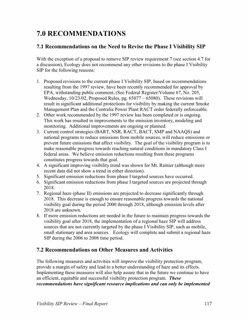
7.0 RECOMMENDATIONS 7.1 Recommendations on the Need to Revise the Phase I Visibility SIP With the exception of a proposal to remove SIP review requirement 7 (see section 4.7 for a discussion), Ecology does not recommend any other revisions to the phase I Visibility SIP for the following reasons: 1. Proposed revisions to the current phase I Visibility SIP, based on recommendations

resulting from the 1997 review, have been recently recommended for approval by EPA, withstanding public comment, (See Federal Register/Volume 67, No. 205, Wednesday, 10/23/02, Proposed Rules, pg. 65077 – 65080). These revisions will result in significant additional protections for visibility by making the current Smoke Management Plan and the Centralia Power Plant RACT order federally enforceable.

2. Other work recommended by the 1997 review has been completed or is ongoing. This work has resulted in improvements to the emission inventory, modeling and monitoring. Additional improvements are ongoing or planned.

3. Current control strategies (BART, NSR, RACT, BACT, SMP and NAAQS) and national programs to reduce emissions from mobile sources, will reduce emissions or prevent future emissions that affect visibility. The goal of the visibility program is to make reasonable progress towards reaching natural conditions in mandatory Class I federal areas. We believe emission reductions resulting from these programs constitutes progress towards that goal.

4. A significant improving visibility trend was shown for Mt. Rainier (although more recent data did not show a trend in either direction).

5. Significant emission reductions from phase I targeted sources have occurred. 6. Significant emission reductions from phase I targeted sources are projected through

2018. 7. Regional haze (phase II) emissions are projected to decrease significantly through

2018. This decrease is enough to ensure reasonable progress towards the national visibility goal during the period 2000 through 2018, although emission levels after 2018 are unknown.

8. If more emission reductions are needed in the future to maintain progress towards the visibility goal after 2018, the implementation of a regional haze SIP will address sources that are not currently targeted by the phase I Visibility SIP, such as mobile, small stationary and area sources. Ecology will complete and submit a regional haze SIP during the 2006 to 2008 time period.

7.2 Recommendations on Other Measures and Activities The following measures and activities will improve the visibility protection program, provide a margin of safety and lead to a better understanding of haze and its effects. Implementing these measures will also help assure that in the future we continue to have an efficient, equitable and successful visibility protection program. These recommendations have significant resource implications and can only be implemented


if adequate funding above and beyond current funding levels is made available. The following measures and activities are listed in descending order of priority. 1. The PSD/NSR rules require air regulatory agencies to conduct cumulative effects

analysis as part of the permit process. To date our capability to conduct cumulative effects analysis has been lacking. It is recommended that Ecology participate in developing a proposal and schedule for developing modeling capabilities to conduct cumulative effects analysis. The proposal and work involved should be a collaborative effort involving resources and expertise of the federal land manager, local air agencies, other air regulatory agencies in neighboring states, EPA, industry and Ecology. Parallel but more critical to developing technical capabilities, is the need to understand and clarify the policy and regulatory implications of cumulative effects analysis. Therefore, it is necessary that a regional policy on the use and implications of cumulative effects analysis be developed prior to the technical capabilities. The Bonneville Power Administration recently completed a cumulative impact study of the effect of several proposed power generating facilities. Much was learned about the technical shortcomings of our ability to conduct such a study. This study could serve as a starting point for discussions. Please see Appendix E for a summary of the study.

2. Continue to support and participate in the WRAP to develop control strategies for the regional haze SIP.

3. Continue to support and participate in the Northwest Regional Modeling Center and their work in developing modeling and emission inventory capabilities for the purpose of understanding the causes and effects of haze in the Pacific Northwest.

4. The Reasonably Available Control Technology program (RACT) is designed to reduce emissions of existing stationary sources. The program allows for reducing emissions for the purpose of mitigating effects to visibility. The RACT for the Centralia Power Plant is an example of how successful this program can be for protecting and improving visibility. However, with the notable exception of the RACT for Centralia, this program has been underutilized for visibility protection. Depending on resource availability and the results of cumulative effects analysis, it is recommended that more resources be dedicated to conducting RACT analysis for all eligible sources that have been shown to impact visibility.

5. Work with EPA and the federal land manager to enhance the IMPROVE monitoring network in Washington state. The current basic network provides 24-hour average aerosol sampling and analysis on a 1 in 3 day schedule. Additional measurement parameters such as continuous high time resolution measurements of meteorology, light scatter, light absorption and various pollutant species, would greatly increase our ability to understand formation of haze and its effects on visibility. Additional monitoring locations in the basic network should also be considered to help us understand the transport of haze.


review of the washington state visibility protection state ... · pdf filereview of the...

Documents