review of income and wealth 2014 doi: 10.1111/roiw

THE INTENSITY AND SHAPE OF INEQUALITY: THE ABG METHOD

OF DISTRIBUTIONAL ANALYSIS

by Louis Chauvel*

University of Luxembourg, IRSEI

Inequality is anisotropic: its intensity varies by income level. We here develop a new tool, the isograph, tofocus on local inequality and illustrate these variations. This method yields three coefficients whichsummarize the shape of inequality: a main coefficient, α, which measures inequality at the median; and twocorrection coefficients, β and γ, which pick up any differential curvature at the top and bottom of thedistribution. The analysis of a set of 232 microdata samples from 41 different countries in the LISdatacenter archive allows us to provide a systematic overview of the properties of the ABG (α β γ)coefficients, which are compared to a set of standard indices including Atkinson indices, generalizedentropy, Wolfson polarization, and the GB2 distribution. This method also provides a smoothing tool thatreveals the differences in the shape of distributions (the strobiloid) and how these have changed over time.

JEL Codes: C16, C46, D31

Keywords: comparisons, distributions, inequality, isograph, polarization, strobiloid

1. Introduction

The analysis of income distribution is central to our understanding of thestructure of inequality and social transformations. In his seminal work on distri-butions, Pareto (1896, p. 99; 1897, pp. 305–24) proposed a leptokurtic distribution,which provided a good approximation to the top of the income hierarchy, andgraphical representations based on incomes (Pareto, 1909, pp. 380–88). Improve-ments have been made since the introduction of the Gini index (Gini, 1914), butthe outdated tools still in use have produced the general conception that inequalityis a single-dimensioned concept, even though these tools can provide a variety ofresults.1 The current contribution intends to show how local inequality can varyalong the income scale. This idea is rooted in the traditional literature on the

Note: I would like to thank two anonymous referees for very fruitful exchanges, Stephen Jenkinsfor several references and a methodological debate on log-logistic distributions, and ConchitaD’Ambrosio for suggestions including polarization measures. This work was supported by the Fondsnational de la recherche, Luxembourg–Social Inequalities Pearl project.

*Correspondence to: Louis Chauvel, University of Luxembourg, IRSEI, Route de Diekirch,L-7201 Walferdange, Luxembourg ([email protected]).

1There have been obvious improvements in our understanding of the socioeconomic processeswhich can generate these Pareto distributions (Gabaix, 2009), and even the double Pareto (Reed, 2001)since the lower tail has this particular shape as well. In this field, general surveys (Cowell, 1995; Kleiberand Kotz, 2003) illustrate the diversity of approaches. Over time, more appropriate and more generalstatistical distributions have been developed, from the Champernowne-I (Champernowne, 1937) andFisk (1961) distributions to the Generalized B of the second kind (GB2), and are becoming standardtools (Jenkins, 2009). In addition, the graphical innovations used to represent distributions have beenreviewed by Dombos (1982), who listed dozens of graphical models.

Review of Income and Wealth 2014DOI: 10.1111/roiw.12161

bs_bs_banner

© 2014 International Association for Research in Income and Wealth

1

problem of ranking income distributions (Atkinson and Bourguignon, 1982;Shorrocks, 1983) and dominance issues (Yitzhaki, 1982), and is consistent with thedevelopment of inequality indices which are sensitive to specific segments ofthe distribution (Atkinson, 1970). Our aim here is to distinguish inequality atthe middle, top, and bottom of the distribution.

Here, the measurement units are individuals and their income is theequivalized household disposable (after tax and transfers) cash income using thesquare root of the number of household members as an equivalence scale. Thisequivalized income is then divided by the median equivalent income of the popu-lation: “medianized equivalized disposable income” (medi) refers to this incomeconcept. Zero or negative points have been excluded from the analyses. The samemethod can be adapted for the analysis of wealth inequality (Jäntti et al., 2013).This is a meaningful question for income distributions, as can be shown in anempirical example with datasets of the LIS database.2 Table 1 shows the quantilesof the income distribution in Israel in 2010 (il10) and the U.S. in 2010 (us10). TheGini coefficients of both series are similar, at 0.387 and 0.371, respectively.However, the comparison of the distributions in Table 1 reveals considerabledifferences. In 2010 in Israel, the fifth percentile level (p5) was 30.1 percent of themedian (p50), and percentile 95 (p95) was 2.95 times the median. Close to themedian there was less inequality in the U.S. than in Israel. However, in the lowerquantiles, the poorer Israeli residents were relatively better off than their U.S.counterparts by far, and the richest percentile p99 was closer to the median inIsrael than in the U.S. Hence, in Israel, there was more inequality around themiddle and less inequality at the extremes of the distribution, with this beingparticularly the case at the bottom. In terms of “general inequality” in 2010, asconventionally reflected in the Gini coefficient, for instance, Israel is slightly moreunequal than the U.S. But in terms of “local” inequality, a notion that can beintuitively defined as a local stretching-out of the distribution, the Israel/U.S.comparison is obviously much more complicated, with there being both more andless inequality across various segments of the income distribution. This kind ofambiguous situation is related to the well-known problem of the comparison ofGini coefficients when the associated Lorenz curves cross each other. We aim toresolve this ambiguity by generalizing the idea of diversity in “local inequality”

2The runs on the Luxembourg Income Study (LIS) database had been completed in September2014; we use the unambiguous two-character iso country codes.

TABLE 1

Percentiles of Incomes in Israel and the U.S. in 2010 and the Difference between Them

p1 p5 p10 p25 p50 p75 p90 p95 p99

il10 0.173 0.301 0.368 0.568 1.000 1.637 2.366 2.945 4.444us10 0.057 0.235 0.362 0.611 1.000 1.531 2.171 2.731 4.501Diff. −0.116 −0.066 −0.006 0.043 0 −0.106 −0.195 −0.214 0.057

Note: Diff. shows the simple percentile level difference between the U.S. and Israel.

Review of Income and Wealth 2014


2

over the income distribution.3 We propose an analysis in terms of the shape ofinequalities that has in general been neglected to date.4

We first discuss how the well-known Champernowne-I–Fisk (CF) distribu-tion (Champernowne, 1937, 1953; Fisk, 1961) can be used as a baseline for localinequality analysis. From this baseline, we propose the “Isograph,” a tool whichrepresents the diversity of local inequality over the income distribution: this revealshow the empirical degree of inequality can be deducted from the CF hypothesis atthe median but with additional curvature at the top and bottom of the distribu-tion.5 We therefore propose an α, β, γ (ABG) method of estimating three inequalityparameters, compatible with the Pareto properties of the tails. The related coeffi-cients are directly interpretable in terms of level-specific measures of inequality: thecentral coefficient (α) measures inequality at the median level, with correctionparameters at the top (β) and bottom (γ). An empirical analysis of 232 datasetsfrom 41 different countries provides estimates of the ABG coefficients. The ABGresults are compared to 30 conventional indicators, and we also compare its abilityto fit empirical distributions with that of the GB2, which can certainly be consid-ered as the most influential distribution in contemporary income analysis(McDonald, 1984; Jenkins, 2009). The advantages of this ABG method are itsability to fit empirical cases, to help us understand the shapes of the distributions(strobiloids), and to provide interpretable coefficients.

2. The CF Distribution as a Baseline

The CF distribution is one of the many statistical laws used to model incomes.We cannot claim that the CF is the best curve—the GB2 provides a better fit sinceit is more flexible with two additional parameters—but it does provide a simpletemplate which is able to pick up changes in local inequality.

In this CF tradition, we can approximate an income distribution as in equa-tion (1). Consider each individual i (i = 1, . . . , n) with income yi > 0; she is abovea proportion pi of individuals (pi is the so-called “standardized quantile” pertainingto income level yi, otherwise called the “fractional rank”) (see Jenkins and VanKerm, 2009). The general quantile distribution expression of the CF of the shapeparameter α (CFα) is particularly simple, provided that we consider medianizedincomes (i.e., income divided by the median), mj = (yj/median):

(1) ln lnm p p

M Xj i i

i i

( ) = −( )( )=

αα

1

or

where Xi = logit(pi) = ln(pi/(1 − pi)) is the logit-rank, and Mi = ln(mi) =ln(yi/median).

3Gabaix (2009) does consider this local degree of inequality, but his topics (mainly the size of cities,firms, and the largest actors on the stock market) lead to a focus on the top of the distribution and noton the whole scale.

4Weeden and Grusky (2012) recently focused on the forms of inequality, but in terms of categoricalgroupings rather than the distribution of economic resources.

5The isograph presents the slope of the “Fisk Graph” (Fisk, 1961, p. 176) that is indeed a logit-logtransformation of the so called Pen’s parade. In the Fisk Graph, compared to the early Fisk proposal of1961, the axes are inversed (like in a quantile function) so that a log income pertains to a logit-rank position.



3

Expression (1) is precisely a CFα, where α measures the degree of inequalityunderstood as the stretching out of the distribution curve.

There are three types of strong arguments which support the use of a CFα asa first approximation to income distributions.

First, with its two-parameter formula (the median and α), the CF is one of themost parsimonious laws with appropriate Pareto-type power-tails at bothextremes, and its formula is remarkably simple. In the CF, log medianized incomeis proportional to the log-odds of the standardized quantile. This parsimony isnotable, and the coefficient α ∈ ]0, 1[ in the CFα has a remarkable role in themeasurement of inequality since its value is the Gini coefficient.6

Second, the CF has a particular position in the field of distributions(McDonald and Xu, 1995, p. 139). It is central in the general tree of beta-typedistributions (Kleiber and Kotz, 2003, p. 188) where GB2 is in this sense thecanopy of the tree and the CF the roots. The CF is a very simplified GB2 where theparameters p and q equal 1. While the CF is much less flexible than the GB2, it doesshare some important features, such as power-tails. The CF is a sub-case of thecomplete Champernowne-II (Champernowne, 1937, 1952) four-parameter distri-bution; Fisk (1961) described this simplified form more generally. He called thisthe “sech2 distribution” (the square of the hyperbolic sequant); it is also called thelog-logistic distribution (Dagum, 1977, 2006; Shoukri et al., 1988).

Third, the CF produces income distributions that are solidly grounded in math-ematical expressions. Here the CF is at a crossroads of different theoretical traditions.In microeconomics, the GB2 (and, as a consequence, the CF which is a GB2 withparameters p = q = 1) can be seen as a result of Parker’s neoclassic model of firmbehavior (Parker, 1999, p. 199; Jenkins, 2009). A number of other theoretical con-structions, such as stochastic processes of income attainment, yield the same distribu-tion. In a proposal from the field of finance, Gabaix (2009) considers stochastic modelsbased on geometric Brownian motion that can generate this type of distribution.

In the social sciences, the balance of power theory of incomes also generates CFlaws. This theory assumes proportionality between the power of income and thepower of rank. Developed societies are socially hierarchized on the basis of rank (ofeducation, prestige, political power, or “value” of any kind) which can be expressedas a standardized rank p in ]0,1[. Each individual i (i = 1, . . . , n) with income yi isabove a proportion pi of individuals and has a proportion of qi = 1 − pi individualsabove him. Since the “power of income” (Champernowne, 1937) is defined asYi = ln(yi), the “power of social rank” (or “logit rank,” or also “logit quantile”) can bedefined as the logit of the rank quantile pi: Xi = ln(pi/qi) = logit(pi).7 Consider twoindividuals (i) and ( j): their difference in power of income ΔY = Yj − Yi, is propor-tional to the difference in their power of rank, ΔX = Xj − Xi. Then, ΔY = αΔX, where

6With his parameterization of the CF cumulative-distribution function F(k; λ; δ) = (1 + λk−δ)−1,k > 0, λ > 0, δ > 1, Dagum (2006, p. 245) demonstrates that Gini = δ −1, where δ > 1 is the shapeparameter of the Fisk distribution. In particular, the α of the ABG is equal to Dagum’s δ −1, so Gini = αprovided that α < 1. In the case of a discrete population, α can be greater than 1: an example is thedistribution of the number of war casualties over the last century (Cederman, 2003), where α isestimated to be 1.5. With income distributions, the highest Gini coefficients are below 0.7.

7Among others, Clementi et al. (2012) log-transform the value of rank, even though the quantile,which is an ]0,1[ interval variable, should be transformed symmetrically (around 0.5), which is what thelogit transformation does, as in Copas (1999).



4

the constant α reflects the intensity of economic inequality in this society. The incomeinequality between (i) and ( j) can thus be derived from the social power of rank:

(2) ln lny y p p p pj i j j i i( ) = −( )( ) −( )( )( )α 1 1

The higher is pi, the greater is the power of social rank; as pi tends to 1, the power ofsocial rank tends to +∞. This could explain why, at the top of the distribution ofprestige, it is strategic to increase rank, as the rewards in terms of logit(quantile) tendto infinity, and the cost of losing rank is very high, and obviously much larger thanthat in the neighborhood of the median. Equally, close to the bottom, gaining/losingrank may have immense consequences in terms of the power of rank and relativeincome. This could explain why Aristotle sees the top of the distribution as danger-ously arrogant and the bottom prone to brutality, while the middle of the scalecorresponds to stability and moderated political attitudes (Aristotle, 1944, p. 329).One important consequence of equation (1) is the existence of a “sling effect,” since,as α increases, the consequences of a percentage change in income can be significantclose to the median but critical at the extremes of the distribution.

In detail, under a CFα distribution, a change of one percentage point in αgenerates an increase of income of about one percentage point near the thirdquartile (X = 0.098), about two percentage points near the ninth decile(X = 2.197), about three near the top 95 percent (X = 2.944), and so on. As theGini coefficient rises, extreme top-incomes gain a much higher percentage in termsof their initial income than do the upper middle class. Symmetrically (in terms oflog), the poor suffer from greater percentage declines in resources than do thelower middle class.

A number of different fields of research (microeconomics, finance, statistics,and social sciences) thus confirm the importance of the CF, although the adequacyof its description of empirical reality remains to be established. The CF is not thebest curve in general: since the GB2 has two additional parameters, it shouldprovide a better fit. Even so, the CF is a parsimonious relevant baseline or templatefor inequality, empirically relevant in the field of income distribution.

3. Measuring Empirical Divergences from the CF Distribution

The analysis of empirical distributions confirms that expression (1) is a first-order approximation that can be improved upon (Appendix 1). I propose theintroduction of an ISO function that generalizes (1) into equation (3) and, therebypicks up the divergence of the empirical curve from the CF hypothesis:

(3) M X X M yi i i i i= ( ) = ( )ISO medianwhere, ln .

Simply, ISO represents the ratio M/X. If ISO(Xi) is a constant (α), (3) simplifies to(1) and the distribution is a CFα that equals the Gini index; the higher the value ofα, the greater is inequality.

In general, the CF distribution hypothesis does somewhat diverge fromreality. Therefore, the isograph representing ISO(Xi) is not a constant and



5

expresses the intensity and the shape of local inequality. The higher is ISO(Xi), thegreater the stretching out of incomes at the logit rank level Xi. The change inISO(Xi) along the distribution measures “local inequality,” which can be thoughtof as the local stretching of the distribution.

The empirical isographs are horizontal lines that are often bent at the twoextremes in different ways. These are obtained empirically by graphing the ISO(0)for each “vingtile” (the 19 slices of five percentiles from 5 to 95 percent). The valueof ISO(0), which can be erratic, is replaced by the average of ISO(p = 0.45) andISO(p = 0.55). The shape of these curves can be explained by taxes, social andredistributive policies which can distort the income curve in such a way that theISO is not constant. The poor can either benefit from income support or be thevictims of extreme social exclusion. The rich can either organize a system ofresource hoarding or accept the development of massive redistributive policies.Therefore, the hypothesis of the strict stability of α along the income scale gener-ally does not hold, since power relations can be stronger or smoother at the topand bottom of the social ladder than near the median.

When the isograph is relatively flat (for example, Finland in 2004), α equalsthe Gini index (0.24 for fi04 in Figure 1). In France, Germany, and Brazil, the CFdistribution hypothesis is an acceptable first-order approximation, but in othercountries the isograph is obviously not constant. The isograph more often revealsa declining level of inequality at the top of the distribution (an ISO with negativeslope). An extreme case is Israel in 2010, with an ISO close to 0.50 at the middle ofthe distribution, similar to Brazil, but much lower at the ends. At the bottom 5percent of the Israeli distribution, ISO(−3) = 0.40, which is similar to Spain andmuch less than the U.S. figure, and at the top 5 percent of the distribution theIsraeli ISO(3) = 0.36, which is very similar to that in the U.S. These findingsillustrate the large movements in local inequality over the income hierarchy. The

za2010

us2010

de2004

fi2004

dk2004

fr1994

jp2008es2004 il2007

ISO(X)

br2006

0.2

0.3

0.4

0.5

0.6

0.7

−4 −2 0 2 4X X = logit(quantile)

Figure 1. The Isograph in 10 Contrasting Cases



6

crossings of the isographs for Israel and the U.S. show extreme inequality close tothe median in Israel balanced by more equality at the extremes. The isograph helpsus to compare inequalities that can shift over the income distribution.

4. The ABG Method of Parametric Estimation of the ISO

The shapes of the 232 isographs (see Appendix 1) show that they can beaccurately captured by only three parameters that I introduce here.8 The isographshapes show that a coefficient pertaining to the level of local inequality close to themedian (α) can be defined along with two shape parameters reflecting isographcurvature at the two extremes. Two correction coefficients β and γ are thereforedetermined, where α + β is the upper asymptote of the ISO and α + γ the lowerasymptote. When γ and β are zero, the distribution is CFα with coefficient whichis the Gini. The added value of this method is to deliver unambiguous interpretableparameters of inequality showing both local inequality at the median, and correc-tions at the top and bottom of the income distribution.9

The parameterization proposed here is compatible with the well-establishedhypothesis that the upper tail has a power-tailed Pareto-type shape (Piketty, 2001),so that the upper asymptote of the ISO(X) function should be a zero-slope line of theequation (Y = α + β). We hypothesize, following Reed (2001), that the lower tail isalso Pareto-shaped. Thus, the lower asymptote of ISO(X) should be the zero-slopeline of the equation (Y = α + γ). Between these two, we have smooth changes.

The parametric expression for these curvatures is based on two functionsθ1 and θ2 related to hyperbolic tangent functions: θ1(X) = tanh(X/2) andθ2(X) = tanh2(X/2) (see Figure 2).

We use two simple linear combinations of these θ functions, B and G, to makethe coefficients easier to interpret. Consider the adjustment of ISO defined by:

8Three plus one parameter of scale that disappears in the case of medianized incomes. GB2 andABG have the same number of parameters, i.e., three of shape and one of scale.

9This aspect is important: the GB2 distribution proposes, in general, a good fit of empiricaldistributions (Jenkins, 2009), but the interpretability of its p and q shape coefficients is unclear.

0.80.60.40.2

00.20.40.60.8

1

5 3 1 1 3 5X = Logit(quan le)

θ1(X)

θ2(X)

1

Figure 2. The θ1 and θ2 functions



7

(4) ISO

where and

X B X G X

B XX X

G XX

i i i( ) = + ( ) + ( )

( ) =( ) + ( ) ( ) = − (

α β γθ θ θ1 2 1

2)) + ( )

( ) = ( ) ( ) = ( )

θ

θ θ

2

1 22

22 2

X

X X X Xand tanh and tanh

then,

(5) M X B X X G X Xi i i i i i= + ( ) + ( )α β γ

where Xi = logit(pi) and Mi = ln(mi).Equation (5) is estimable as Xi and the functions are known, and there are no

collinearity issues. The α, β, γ can be estimated in a single multivariate OLSregression without a constant. In the results:

• the coefficient α measures inequality close to the median;• β characterizes the additional inequality at the top of the distribution, β

being positive when the rich are richer than in the CFα, so that the upper tailis stretched; and

• γ characterizes the additional inequality at the bottom of the distribution,with γ being positive when the poor are poorer than in the CFα.

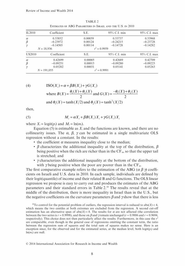
The first comparative example refers to the estimation of the ABG (α β γ) coeffi-cients on Israeli and U.S. data in 2010. In each sample, individuals are defined bytheir logit(quantile) of income and their related B and G functions. The OLS linearregression we propose is easy to carry out and produces the estimates of the ABGparameters and their standard errors in Table 2.10 The results reveal that at themiddle of the distribution, there is more inequality in Israel than in the U.S., butthe negative coefficients on the curvature parameters β and γ show that there is less

10To control for the potential problem of outliers, the regression interval is reduced to abs(X) < 4,which means the two centiles at both extremes are excluded from the regression. A second cut-offestimation has an alternative span of abs(X) < 8. The results for α are not affected (the correlationbetween the two series is r = 0.9998), and those on β and γ remain unchanged (r = 0.9886 and r = 0.9694,respectively). This choice does not then particularly affect the results. Furthermore, in this case the r2

are comparable, even though in the general case of regressions omitting the constant term, the ratiobetween the regression sum of squares and the total sum of squares makes no sense. Here is anexception since, for the observed and for the estimated series, at the median level, both logit(pi) andln(mi) are null.

TABLE 2

Estimates of ABG Parameters in Israel and the U.S. in 2010

IL2010 Coefficient S.E. 95% C.I. min 95% C.I. max

α 0.53852 0.00059 0.53737 0.53968β −0.23972 0.00124 −0.24215 −0.23728γ −0.14505 0.00114 −0.14728 −0.14282

N = 18,936 r2 = 0.9959

US2010 Coefficient S.E. 95% C.I. min 95% C.I. max

α 0.42699 0.00005 0.42689 0.42709β −0.09251 0.00015 −0.09280 −0.09223γ 0.05202 0.00031 0.05141 0.05263

N = 191,055 r2 = 0.9991



8

inequality in Israel at the extremes than in the U.S. (α + β and α + γ are bothsmaller in Israel). These results reflect the complex comparison of the U.S. to Israelin Table 1, and underline the particular polarization in Israel (García-Fernándezet al., 2013); conversely, in the U.S., there is extreme inequality at the bottom (highvalues of γ) with very low values for the poorest centiles.

In the empirical analysis of 232 cases, β and γ are always much smaller thanα (see Appendix 2): in this case, the CF distribution is an acceptable simplifiedfirst-order hypothesis, and β and γ are correction coefficients. When β (γ) is 1percent higher, the ISO(X) function increases by 1 percent at the upper (lower)asymptote. The ABG has three shape parameters, plus one scale parameter derivedfrom the ISO(X) estimation function (6).11

In this decomposition, α, α + β and α + γ are the inequality measures at themedian, top, and bottom of the distribution, respectively, and are homogeneouswith the Gini coefficient in the sense that the upper tail of a distribution ofcoefficient (α + β) is similar to a CFα+β.

There is no analytic expression for these measures since they come from aregression of M on the functions XB(X) and XG(X). Similarly, equation (5) yields nosimple cumulative distribution function, but when β = γ = 0, equation (5) correspondsto a CFα distribution. The solutions are numerical whenever β or γ is non-zero.

The coefficients α, β, and γ satisfy most of the criteria of the appropriateinequality measures (see Jenkins, 1991, 1995; Cowell and Jenkins, 1995; Haughtonand Khandker, 2009, p. 105):

• Mean independence: a proportional change in incomes does not affect themeasures.

• Population-size independence: all else equal, a change in population sizedoes not affect the measures.

• Symmetry: if individuals (a) and (b) exchange their income levels, the mea-sures are not affected.

• Decomposability: this possibility is not exploited in the limits of the currentpaper, but covariates can be added to model (5) so that nested models canshow how inequality results from inter- or intra-group variance, with the“group” being potentially defined by gender, education, ethno-culturalorigins, and so on.

• Pigou–Dalton Transfer (PDT) sensitivity: the ABG method and the idea oflocal inequalities is not compatible with the strict PDT principle whichclaims that inequality falls when a richer individual (a) gives a part of herincome to a poorer individual (b), provided that the hierarchy is notinverted. If (a) and (b) are above the median, and if the local inequalitybetween (a) and (b) falls, inequality between the median and (b) increasessince (b) gets richer, and thus further from the median. Such a transfer isambiguous at the local level: even if the stretching between (a) and (b) islower, meaning less inequality, the stretching between (b) and the medianincreases, meaning more inequality. The ABG method does satisfy, in any

11In the conventional literature, this is a 4-parameter distribution, but with medianized income thetraditional b coefficient is automatically set to 1.



9

case, a weaker form of the PDT principle provided that (a) is above themedian and (b) below it, and that they remain in this order relative to themedian after the transfer.

5. Comparative Analysis of 232 Datasets and Inequality Measures

Sections 5 and 6 analyze the performance of the ABG method compared toexisting indicators (Section 5) and to the well-known GB2 distribution (Section 6).The added value of the ABG method over other measures is illustrated via itscomparison to more customary inequality indices on a set of 232 harmonizedmicrodata files covering 41 countries provided by the LIS datacenter.

The first result is that the absolute values of β and γ are small compared tothat of α, so that α + β and α + γ are always in the interval [0,1]. The signs of β andγ can be positive or negative (Figure 3), and the point β = 0 and γ = 0 is in themiddle of the range of βs and γs.

We can compare the three ABG indices to other standardized inequality mea-sures. These selected indicators are well-known or based on simple income ratios. Weconsider ISO indicators at five different levels. In addition, the sizes (as a proportion inthe total population) of five income classes are included: the poor (po), lower middleclass (mcl), middle class (mc), upper middle class (mcu), and the rich (ri). Overall, ouranalysis covers a set of 30 variables and 232 data samples (see Appendix 2a).

One important question is the relative position of the ABG parameters in thefield of inequality measures. A first answer is given by an analysis of the correlationmatrix of these indicators (Appendix 3): there is a very strong relation between α

at1987at1994

at1995

at1997at2000

at2004

au1981

au1985au1989

au1995

au2001

au2003be1985

be1988

be1992

be1995

be1997

be2000

br2006

br2009

br2011

ca1971ca1975ca1981ca1987

ca1991

ca1994

ca1997ca1998ca2000

ca2004

ca2007ca2010

ch1982ch1992

ch2000

ch2002

ch2004

cn2002

co2004

co2007co2010

cz1992

cz1996cz2004

de1973de1978

de1981

de1983de1984

de1989de1994

de2000 de2004

de2007

de2010

dk1987

dk1992dk1995dk2000dk2004

dk2007dk2010

ee2000

ee2004

ee2007

ee2010

es1980

es1985

es1990

es1995

es2000

es2004es2007

es2010

fi1987fi1991

fi1995

fi2000

fi2004

fi2007fi2010

fr1978

fr1984

fr1989fr1994

fr2000 fr2005fr2010

gr1995

gr2000

gr2004

gr2007

gr2010

gt2006

hu1991

hu1994

hu1999

hu2005ie1987

ie1994

ie1995

ie1996ie2000

ie2004

ie2007

ie2010il1979

il1986

il1992

il1997

il2001

il2005

il2007

il2010

in2004

is2004is2007

is2010

it1986

it1987

it1989

it1991

it1993

it1995it1998

it2000

it2004it2008

it2010

jp2008kr2006

lu1985

lu1991

lu1994

lu1997

lu2000

lu2004

lu2007

lu2010

mx1984mx1989

mx1992

mx1994mx1996

mx1998mx2000

mx2002mx2004

mx2008

mx2010

nl1983

nl1987 nl1990 nl1993nl1999

nl2004nl2007nl2010 no1979

no1986no1991no1995

no2000no2004no2007no2010

pe2004

pl1986

pl1992 pl1995pl1999pl2004

pl2007pl2010

ro1995

ro1997

ru2000ru2004

ru2007

ru2010

se1967

se1975

se1981se1987

se1992

se1995

se2000

se2005

si1997 si1999

si2004

si2007

si2010sk1992

sk1996

sk2004

sk2007

sk2010tw1981

tw1986tw1991 tw1995tw1997

tw2000tw2005tw2007 tw2010

uk1969

uk1974

uk1979

uk1986uk1991uk1994

uk1995uk1999

uk2004

uk2007

uk2010 us1974us1979

us1986

us1991

us1994

us1997us2000

us2004

us2007 us2010

uy2004

za2008

za2010

–0.2

–0.1

00.

10.

2be

t

–0.2 –0.1 0 0.1 0.2gam

Value of β

Value of γ

Figure 3. The Relation between β and γ



10

and the Gini index (r = +0.95), thus confirming the relation of these two inequalitymeasures when the CFα approximation is acceptable. More generally, most of themeasures correlate well with α. This is good news for the ABG method, but thenwhat is its intrinsic added value? A second answer is that we also see interestingcorrelations for the β and γ coefficients, which thus provide complementary infor-mation to α: the degree to which inequality moves at the top and at the bottom ofthe distribution. A third more systematic answer comes from the principal com-ponent analysis (PCA) of the whole table (see Appendix 2a). The first axis of thePCA (69 percent of the total variance) reveals the similar nature of many inequal-ity measures, including α; this axis picks up inequality intensity. The α coefficientappears on the first axis of the PCA, along with the Atkinson index with param-eters 1 and 1⁄2, the generalized entropy with parameters 1 and 0, the Gini coeffi-cient, a number of quantile ratios, as well as the Wolfson polarization index.12 Thisconfirms that α is a new inequality parameter which is highly correlated with themain inequality measures, but is more sensitive (like the Wolfson index) to themedian of the distribution (see Appendix 2a for details).

The role of β and γ becomes apparent on axes 2 and 3 (12 and 7 percent of thevariance, respectively), which reveal the shape of inequality but not its intensity. Onthe second PCA axis, β and γ are strongly correlated in the same direction as the twomeasures of the over-elongation of the extreme deciles compared to the quartiles:

pp quartile decile median quartile and its symmetr251050 1 1 1= ( ) ( ), iic

pp decile quartile quartile median

,

.907550 9 3 3= ( ) ( )

The correlation with the upper and lower middle class sizes is negative: the elon-gation at the top (resp. bottom) implies a smaller upper (resp. lower) middle classthat is stretched out. Positive values on the second axis reflect greater inequality atthe extremes. Here, the generalized entropy index with parameter 2 is morestrongly correlated on axis 2 than are the other traditional measures.

Axis 3 shows the difference between γ and β, along with the contrast betweenpp251050 and pp907550. On this axis, the generalized entropy index with param-eter 1 and the Atkinson index with parameter 2 are located on the same side of axis3 as γ. All of these indicators are relatively more sensitive to inequality at thebottom. Conversely, the generalized entropy index with parameter 2, located on thesame side of axis 3 as β, is sensitive to inequality at the top. Therefore, β and γ pickup salient features of the distribution that are less-well detected by other measures.

We can also ask whether the ABG method provides a better assessment ofpolarization than the Wolfson index (Wolfson, 1986). A simple measurement ofmiddle class hollowing, rpol ratio, is the of the sum of the size of upper middle classand lower middle class by central middle class, the one closer to the median. Thelinear correlation matrix shows that, in terms of r2, the Wolfson index is indeed betterthan the Gini in predicting the rpol ratio, but α is even better. A nested model of the232 datasets with respect to middle-class polarization (rpol) compares the perfor-mances of the Gini, the Wolfson, and the α coefficients (see Appendix 2a). In general,

12The Wolfson index is chosen here because it is standard in the literature, even though morereliable propositions exist (Alderson et al., 2005; Chakravarty and D’Ambrosio, 2010).



11

for the different aspects of inequality measurement, the ABG method offers interpre-table parameters that generally outperform the other methods in terms of the descrip-tion of the distribution and the size of income classes.

6. How do the ABG Distribution and GB2 Perform?

Another aspect of the ABG method is its distributional shape: the threeparameters describe a distribution that is tailored to fit the observed data. Howdoes ABG perform in this respect? In the contemporary income-distribution lit-erature, the GB2 is the leading contender for the best measure (Jenkins, 2009; Grafand Nedyalkova, 2014). This distribution is particular in the universe of beta-typelaws: it is the most general, as many other distributions are special cases. It has fourparameters, one of scale (b) and three of shape (a, p, q), which is the same numberas the ABG distribution, provided that we consider equation (5) as a generalexpression of an empirical distribution where the fourth parameter (size) is themedian. In terms of microeconomic theory, the GB2 results from a simple modelof firm behavior (Parker, 1999), and is acknowledged for its flexibility. Statisticaltools to estimate the GB2 parameters are easily available.

To compare the respective performances of ABG and of GB2, we considerthe divergence from the empirical observed distribution (OBS) of ABG, GB2,and CF. This is not an easy task since the GB2 predicted values are based on aknown cumulative distribution function and an unknown quantile function(although its estimation via simulation is possible) and the ABG provides aquantile function. Our solution here is to compare the predicted values of each“vingtile” level of logged incomes for four quantile functions: the empirical dis-tribution as the target, the GB2 and ABG as competitors, and the CFα as thebaseline. As they have more parameters (and are thus more flexible), the GB2 andABG provide a better fit to the OBS than does CFα. One measurement of thegoodness of fit is the ra

2 (the adjusted coefficient of determination): the higher isra

2, the better the fit to the OBS. The most difficult issue concerns the estimationof the GB2 parameters (a, b, p, q) for the 232 samples; here the STATA gb2lfitprogram only converged quickly in 205 cases. The maximum number of itera-tions was set to 6, since convergences after 7 or more iterations are exceptionaland may be considered as outliers.

Our analysis is restricted to the 205 convergent cases. We have for eachcountry the vectors of 19 vingtiles of log income levels for the CF-Gini (lincq),ABG (linaq), GB2 (lingq), and the empirical OBS distribution (linoq: o forobserved), with q = 1 . . . 19. The adjusted ra

2 of the OLS regression of (lincq) on(linoq) reflects the quality of the CF hypothesis: the higher the value, the better thefit (Table 3). On average, the CF is a good first-order approximation ra

2 0 996=( ). ,and both GB2 and ABG improve the fit further, with a clear advantage for thelatter. In 67.8 percent of cases, GB2 is better than CF, but ABG outperforms CFin 85.8 percent of cases and GB2 in 76.5 percent.

We can explain the better fit of the ABG methodology. We simulated manyGB2 distributions from the shape parameters a, p, and q, each randomly-defined;we then fitted these with the ABG method, and found no cases where the β and γ



12

coefficients were strongly negative at the same time. This means that stronglypolarized distributions such as than in Israel in 2010, with its stretched middle classand relatively more equality at the top and the bottom, cannot be generated fromthe GB2 distribution. The GB2 is flexible, but does not cover every case, and inparticular those where β and γ are both positive. This means that the GB2 withparameters a, p, q is less general than the ABG with coefficients α, β, and γ, whichis more flexible with the same number of parameters.

The GB2 is a good tool, and has the advantage of being theoretically more solidand mathematically purer than the ABG, but does nonetheless present some difficul-ties. The interpretation of the GB2 parameters a, p, q is not obvious, with theexception of the case where p = q = 1. The ABG method is on the other hand lesstheoretically-satisfying: it has no simple analytical expression, is very empirical, and isa computer-oriented fitting tool. However, ABG produces three easy to estimate andinterpret coefficients that make sense of the distribution of inequality, with values thatare compatible with the Gini tradition since α = Gini if β and γ are close to 0.

7. Representing the Shape of the Income Distribution: The Strobiloid

The ABG decomposition provides a method for smoothing the empiricalquantile distribution function. If, for instance, we are interested in the architectureof societies represented by the distribution density curve, as in the seminal work ofPareto (1897, p. 315), we can plot income on the vertical hierarchical axis and thedensity value on the horizontal axis, as in Figure 4. One convenient way of stan-dardizing the representations, for comparison purposes, is to normalize the incomecurve. With both the medianization of income and the normalization of the surfaceto 1 (so that it defines the density of the distribution), we can superpose the curvesfor different periods or countries. This is the strobiloid representation (Chauvel,1995; Lipietz, 1996; Chauvel, 2013).13

These empirical strobiloids reveal the diversity of income distributions acrosscountries and reflect the change in socioeconomic architecture within countries. Inthe strobiloid, the wider the curve, the more individuals there are at this level of thegraph: middle-class societies will have a large belly (Denmark), whereas in thecontemporary American distribution a large proportion of the population is close

13The strobiloid is based on Pareto’s (1897, p. 313) idea that the shape is one of an arrow or of aspinning top. This representation, which is similar to Pareto’s first representations of the income pyramid,allows us to make 2 • 2 comparisons over countries, time, etc. Nielsen (2007) provides an overview ofPareto’s legacy, and considers why this has generally been neglected in the social sciences.

TABLE 3

Frequency of a Better Fit of Distribution D1 Compared to D2 (%) on 205 Samples (27excluded cases with more than 6 iterations)

Average Adjusted r2

of the fit of OBSPair Comparison: % of Cases Where the

Fit of A is Worse Than That of B

CF 0.9959 CF worse than GB2: 67.8%GB2 0.9975 GB2 worse than ABG: 76.5%ABG 0.9989 CF worse than ABG: 85.8%



13

to the bottom. Kernel smoothing can produce similar curves, but the ABG methodrelies on a Pareto power-tail compatible methodology to produce interpretableparameters. This new tool allows the country and time comparison of the consid-erable developments in the intensity and shape of inequality.

The strobiloid shows that incomes in Denmark in 1987 are generally “moreequal” than elsewhere, although the particularity of Denmark (due to its low α andhigh positive γ) is its lack of rich rather than its lack of poor, with some of the latterbeing stretched far to the bottom of the distribution. The bottom part of the curvein Germany in 1983 shows the same level of inequality as in Denmark in 1987 (ascan be seen from the isograph in Figure 5), although there is more inequality inGermany in 1983 for higher income levels. In terms of public policy, the structureof Germany in 1983 is a particular model of homogeneity below the median witha high implicit level of minimum income.

The French distribution is fairly common in Europe and is stable over the periodunder consideration. On the contrary, there is a strong polarization trend in the U.K.,which is converging to the onion-shaped strobiloid of the U.S. The U.S. itself has aneven more pronounced onion shape with increasing inequality. One feature of thisshape is less the extreme values at the top but rather the lower values with a very highγ. Israel, the final case, may be the most symbolic in terms of the shift from a moreequal to a far less equal distribution, with one particular feature: a steady decline in

dk1987 dk20100

12

34

–1 0 1

de1978 de2010

01

23

4

–1 0 1

fr1978 fr2010

01

23

4

–1 0 1

uk1979 uk2010

01

23

4

–1 0 1

us1979 us2010

01

23

4

–1 0 1

il1979 il2010

01

23

4

–1 0 1Density

Income

Figure 4. Six typical strobiloids (Denmark, Germany, France, U.K., U.S., and Israel)

Note: The strobiloid shows the income hierarchy (on the vertical axis, 1 = median). The curve islarger (horizontal axis) when the density at this level of income is higher: Many individuals are atthe intermediate level near to the median and their number diminishes at the top and at the bottom. Thus,in strobiloids with a larger belly, the intermediate middle class is larger with a more equal distribution.



14

the median class of incomes with a relatively strong minimum-income scheme,leading to the development of an unprecedented arrowhead-shaped curve. Israelappears then as an extreme case of rapid polarization over recent decades, which isconfirmed by the isograph in Figure 5. A broader international comparison revealsthe diversity of distributions across countries (Appendix 4).

8. Conclusion

The ABG methodology represents progress in terms of both measurement andgraphical representation (CF curve, isograph and strobiloid) of the diversity ofinequality at different levels of income, since in many cases inequality is anisotropicalong the income scale. In terms of public policies, it can reveal useful informationabout the different dynamics of inequality, where inequality at the median, α, can beanalyzed in parallel with that at the extremes described by β and γ.

The ABG approach relies on an easy-to-use family of distributions to modelincome distributions. It can be used, for example, to model extremely unequaldistributions such as Zipf laws (Gabaix, 1999), which are extreme Paretodistributions with α close to 1. It also helps us to understand why the Ginicoefficient can pose problems when the isograph is far from being a constant (whenβ and γ differ greatly from 0).

dk1987dk2010

de1978de2010

fr1978fr2010

uk1979uk2010

us1979us2010

il1979il2010

0.2

0.3

0.4

0.5

0.6

0.2

0.3

0.4

0.5

0.6

–4 –2 0 2 4 –4 –2 0 2 4 –4 –2 0 2 4

Graphs by col X = logit(quantile)

ISO(X)

Figure 5. Isographs for Six Typical Countries

Note: The dots represent the empirical values and the lines are the fitted isographs (ABGmethod). For each country, two periods are considered: the dashed line and white dots pertain to theolder years, the full line and gray dots refer to more recent years. The higher the curve at a given levelof X (logit rank), the greater are the income inequalities at this level. Israel over 1986–2010 is an obviouscase of extreme polarization.



15

In this approach, the magnitudes of ranks and incomes, defined bylogit(quantile) and log(income), are almost linearly-related. The logit(quantile)may therefore be an important tool for the measurement of inequality, and couldbe used in other fields such as income volatility and more generally in stratificationresearch. The further development of the ABG should include the analysis ofstatistical significance and group decomposability. As the ABG coefficients comefrom linear regressions, we can add control variables to understand how the gapsbetween groups (education, gender, etc.) contribute to overall inequality. Finally,we also need further analysis of isograph shapes when the absolute value of X isover 5, for the very rich and very poor.

The results that we presented here can also be found with more traditionaltools, but the α, β, γ ABG method, the CF and the isograph, and the associatedstrobiloid, represent more systematic and easier to use tools for the detection ofparticular shapes, propose better measures of the income distribution, and help usto better understand the anisotropy of inequality.

References

Alderson, A. S., J. Beckfield, and F. Nielsen, “Exactly How Has Income Inequality Changed? Patternsof Distributional Change in Core Societies,” International Journal of Comparative Sociology, 46,405–23, 2005.

Aristotle, Politics, Loeb Classical Library, Harvard University Press, Cambridge, MA, 1944.Atkinson, A. B., “On the Measurement of Inequality,” Journal of Economic Theory, 2, 244–63, 1970.Atkinson, A. B. and F. Bourguignon, “The Comparison of Multi-Dimensioned Distributions of

Economic Status,” Review of Economic Studies, 49, 183–201, 1982.Cederman, L.-E., “Modeling the Size of Wars: From Billiard Balls to Sandpiles,” American Political

Science Review, 97, 135–50, 2003.Chakravarty, S. R. and C. D’Ambrosio, “Polarization Orderings of Income Distributions,” Review of

Income and Wealth, 56, 47–64, 2010.Champernowne, D. G., “The Theory of Income Distribution,” Econometrica, 5, 379–81, 1937.———, “The Graduation of Income Distributions,” Econometrica, 20, 591–615, 1952.———, “A Model of Income Distribution,” Economic Journal, 63, 318–51, 1953.Chauvel, L., “Inégalités singulières et plurielles: l’évolution de la courbe de répartition des revenus,”

Revue de l’OFCE, 55, 211–40, 1995.———, “Welfare Regimes, Cohorts and the Middle Classes,” in J. Gornick and M. Jäntti (eds),

Economic Inequality in Cross-National Perspective, Stanford University Press, Stanford, CA,115–41, 2013.

Clementi, F., M. Gallegati, and G. Kaniadakis, “A New Model of Income Distribution: Theκ-Generalized Distribution,” Journal of Economics, 105, 63–91, 2012.

Copas, J., “The Effectiveness of Risk Scores: The Logit Rank Plot Quick View,” Journal of the RoyalStatistical Society. Series C (Applied Statistics), 48, 165–83, 1999.

Cowell, F. A., Measuring Inequality, 2nd edition, Harvester Wheatsheaf, Hemel Hempstead, 1995.Cowell, F. A. and S. P. Jenkins, “How Much Inequality Can We Explain? A Methodology and an

Application to the USA,” Economic Journal, 105, 421–30, 1995.Dagum, C., “A New Model of Personal Income Distribution: Specification and Estimation,” Economie

Appliquée, 30, 413–36, 1977.———, “Wealth Distribution Models: Analysis and Applications,” Statistica, 6, 235–68, 2006.Dombos, P., “Some Ways of Examining Dimensional Distributions,” Acta Sociologica, 25, 49–64,

1982.Fisk, P. R., “The Graduation of Income Distributions,” Econometrica, 29, 171–85, 1961.Gabaix, X., “Zipf’s Law for Cities: An Explanation,” Quarterly Journal of Economics, 114, 739–67, 1999.———, “Power Laws in Economics and Finance,” Annual Review of Economics, 1, 255–94, 2009.García-Fernández, R. M., D. Gottlieb, and F. Palacios-González, “Polarization, Growth and Social

Policy in the Case of Israel, 1997–2008,” Economics Discussion Papers, No. 2012-55, Kiel Institutefor the World Economy, 2013.

Gini, C., “Sulla misura della concentrazione e della variabilità dei caratteri,” Atti del Reale IstitutoVeneto di Scienze, Lettere ed Arti, LXXIII, parte II, 73, 1203–48, 1914.



16

Graf, M. and D. Nedyalkova, “Modeling of Income and Indicators of Poverty and Social Exclusionusing the Generalized B Distribution of the Second Kind,” Review of Income and Wealth, 60,821–42, 2014.

Haughton, J. H. and S. R. Khandker, Handbook on Poverty and Inequality, The World Bank, Wash-ington DC, 2009.

Jäntti, M., E. Sierminska, and P. Van Kerm, “The Joint Distribution of Income and Wealth,” in J.Gornick and M. Jäntti (eds), Economic Inequality in Cross-National Perspective, Stanford Univer-sity Press, Stanford, CA, 312–33, 2013.

Jenkins, S. P., “The Measurement of Income Inequality,” in L. Osberg (ed.), Economic Inequality andPoverty: International Perspectives, M. E. Sharpe, Armonk, NY, 3–38, 1991.

———, “Accounting for Inequality Trends: Decomposition Analyses for the UK, 1971–86,”Economica, 62, 29–63, 1995.

———, “Distributionally-Sensitive Inequality Indices and the GB2 Income Distribution,” Review ofIncome and Wealth, 55, 392–8, 2009.

Jenkins, S. P. and P. Van Kerm, “Decomposition of Inequality Change into Pro-Poor Growth andMobility Components,” CEPS/INSTEAD, Differdange, Luxembourg, 2009.

Kleiber, C. and S. Kotz, Statistical Size Distributions in Economics and Actuarial Sciences, John Wiley,Hoboken, NJ, 2003.

Lipietz, A., La Société en sablier. Le partage du travail contre la déchirure sociale, La Découverte, Paris,1996.

McDonald, J., “Some Generalized Functions for the Size Distribution of Income,” Econometrica, 52,647–63, 1984.

McDonald, J. B. and Y. Xu, “A Generalization of the Beta Distribution with Applications,” Journal ofEconometrics, 66, 133–52, 1995.

Nielsen, F., “Economic Inequality, Pareto, and Sociology: The Route Not Taken,” American Behav-ioral Scientist, 50, 619–38, 2007.

Pareto, V., “La courbe des revenus,” Le Monde economique, July, 99–100, 1896.———, Cours d’économie politique, Rouge, Lausanne, 1897.———, Manuel d’économie politique, V. Giard et E. Brière, Paris, 1909.Parker, S. C., “The Generalized Beta as a Model for the Distribution of Earnings,” Economics Letters,

62, 197–200, 1999.Piketty, T., Les hauts revenus en France au XX ème siècle. Inégalités et redistributions, 1901–1998,

Grasset, Paris, 2001.Reed, W. J., “The Pareto, Zipf and Other Power Laws,” Economics Letters, 74, 15–19, 2001.Shorrocks, A. F., “Ranking Income Distributions,” Economica, 50, 3–17, 1983.Shoukri, M. M., I. U. M. Mian, and D. S. Tracy, “Sampling Properties of Estimators of the Log-

Logistic Distribution with Application to Canadian Precipitation Data,” The Canadian Journal ofStatistics/La Revue Canadienne de Statistique, 16, 223–36, 1988.

Weeden, K. A. and D. B. Grusky, “The Three Worlds of Inequality,” American Journal of Sociology,117, 1723–85, 2012.

Wolfson, M. C., “Stasis amid Change: Income Inequality in Canada, 1965–1983,” Review of Incomeand Wealth, 32, 337–69, 1986.

Yitzhaki, S., “Stochastic Dominance, Mean Variance, and Gini’s Mean Difference,” American Eco-nomic Review, 72, 178–85, 1982.

Supporting Information

Additional Supporting Information may be found in the online version of this article at thepublisher’s web-site:

Appendix 1: Figure of 232 IsographsAppendix 2: Table of 30 Inequality IndicesAppendix 2a: Comparisons of 30 indicators of inequality samples and a Principal Component

Analysis PCA on 232 LIS samplesAppendix 3: General Correlation Matrix of 30 Inequality IndicatorsAppendix 4: Figure of 32 Countries StrobiloidsAppendix 5: Distribution Simulator for ABG

A program for the ABG method is available to Stata users who can install the program directly bytyping: ssc install gb2fit.



17

review of income and wealth 2014 doi: 10.1111/roiw

Documents