reverse engineering utilizing - school of computinggermain/thesis.pdf · reverse engineering...
TRANSCRIPT

REVERSE ENGINEERING UTILIZING
DOMAIN SPECIFIC KNOWLEDGE
by
H. James de St. Germain
A dissertation submitted to the faculty of
The University of Utah
in partial fulfillment of the requirements for the degree of
Doctor of Philosophy
in
Computer Science
School of Computing
The University of Utah
December 2002

Copyright H. James de St. Germain 2002
All Rights Reserved

THE UNIVERSITY OF UTAH GRADUATE SCHOOL
SUPERVISORY COMMITTEE APPROVAL
of a dissertation submitted by
H. James de St. Germain
This dissertation has been read by each member of the following supervisory committee
and by majority vote has been found to be satisfactory.
______________________ ______________________________________
Chair: William B. Thompson
______________________ ______________________________________
Richard F. Riesenfeld
______________________ ______________________________________
Christopher R. Johnson
______________________ ______________________________________
Samuel H. Drake
______________________ ______________________________________
Don Brown

THE UNIVERSITY OF UTAH GRADUATE SCHOOL
FINAL READING APPROVAL
To the Graduate Council of the University of Utah:
I have read the dissertation of H. James de St. Germain in its final
form and have found that (1) its format, citations, and bibliographic style are consistent
and acceptable; (2) its illustrative materials including figures, tables, and charts are in
place; and (3) the final manuscript is satisfactory to the supervisory committee and is
ready for submission to The Graduate School.
____________________________ _________________________________
Date William B. Thompson
Chair: Supervisory Committee
Approved for the Major Department
_______________________________________
Thomas C. Henderson
Director
Approved for the Graduate Council
_______________________________________
David S. Chapman
Dean of The Graduate School

ABSTRACT
Reverse engineering is the process of defining and instantiating a model based on
the measurements taken from an exemplar object. The measurement (or data sensing)
process is prone to random and systematic errors and often fails to sense the object in a
manner consistent with the intended functionality of the object's design. Therefore a
model fit directly to the data will not faithfully capture the geometry of the part (the
form), nor the relationships among features of the part (the function) as originally
specified by the designer.
Manmade objects are often well defined, following specific rules and structures
based on perceived pragmatics. This is especially true in the case of mechanical two and
a half dimensional (2.5D) machined parts. Because of the high accuracy needs of this
domain, reverse engineering techniques using generic primitives are inappropriate. This
dissertation asserts that an understanding of common design practices and
manufacturing knowledge specific to 2.5D machining can and should be used to guide
the reverse engineering process in order to achieve higher accuracy models.
To this end, reverse engineering is characterized as a constrained optimization
problem. Logical laws of form are encoded as constraints in order to coerce new models
to emulate the structure common to this genus of parts while best approximating the
sensed data. A technique has been created to automatically hypothesize likely
constraints that should hold on a hypothesized model. These constraints drive a DOF
reduction process on the model and are further encoded as penalty functions during the
model optimization. The entire process is formulated in a manner consistent with
modern optimization techniques.

For Dad
(and you too Mom)

TABLE OF CONTENTS
ABSTRACT ....................................................................................................................... iv
LIST OF FIGURES ......................................................................................................... viii
LIST OF TABLES ............................................................................................................. ix
ACKNOWLEDGEMENTS .................................................................................................x
1 INTRODUCTION ........................................................................................................1
1.1 Thesis ................................................................................................................. 3
1.2 Goals and Validation Techniques ...................................................................... 4
1.3 Reverse Engineering Process ............................................................................. 4
1.4 Artifacts .............................................................................................................. 6
1.5 Optimization Over Constraints .......................................................................... 7
1.6 Overview ............................................................................................................ 7
2 BACKGROUND ..........................................................................................................9
2.1 Reverse Engineering in the Field of Manufacturing .......................................... 9
2.2 Modeling .......................................................................................................... 11
2.3 Data Segmentation ........................................................................................... 14
2.4 Data Fitting ...................................................................................................... 15
2.5 Dimensioning and Tolerance Information ....................................................... 18
2.6 Feature-Based Design ...................................................................................... 20
2.7 Geometric Constraints ...................................................................................... 22
2.8 Sensors and Scanning ....................................................................................... 24
2.9 Optimization ..................................................................................................... 28
3 DESIGN ARTIFACTS, CONSTRAINTS, AND REVERSE ENGINEERING ........39
3.1 Reverse Engineering an Exemplar Part............................................................ 40
3.2 Design and Manufacturing in the Domain of 2.5D Axis Machining ............... 49
3.3 The Advantages Attained by Using Constraints .............................................. 50
3.4 Taxonomy of Constraints ................................................................................. 52
3.5 Overview .......................................................................................................... 58
4 CONSTRAINT FORMULATION FOR MODEL OPTIMIZATION .......................60
4.1 Problem Formulation ....................................................................................... 61
4.2 Constraint Representation ................................................................................ 64
4.3 Construction of Primitives ............................................................................... 65
4.4 Defining the Reduced Degrees of Freedom Model.......................................... 67

vii
4.5 The Optimization Function .............................................................................. 70
4.6 DOF Reduction Example ................................................................................. 71
4.7 Penalty Function Example ............................................................................... 74
4.8 Discussion of Under and Over Constrained Geometry .................................... 74
4.9 Constraint Formulation Summary .................................................................... 76
5 AUTOMATIC CONSTRAINT ACQUISITION .......................................................78
5.1 Manufacturing and Design Knowledge ........................................................... 79
5.2 Parametric Equivalence .................................................................................... 80
5.3 Hypothesis Based on Geometric Considerations ............................................. 84
5.4 A Word of Caution ........................................................................................... 85
6 THE REVERSE ENGINEERING PROCESS QUANTIFIED ..................................87
6.1 Desired Results ................................................................................................ 89
6.2 The Parts........................................................................................................... 92
6.3 The Process ...................................................................................................... 96
6.4 Data Acquisition............................................................................................... 96
6.5 Initial Segmentation and Plane Fitting ............................................................. 97
6.6 Initial Feature by Feature Estimation ............................................................... 97
6.7 Automatic Constraint Acquisition.................................................................... 98
6.8 DOF Reduction and Boundary Function Creation ......................................... 100
6.9 Error Analysis ................................................................................................ 101
6.10 Summary ........................................................................................................ 105
7 CONCLUSION.........................................................................................................107
7.1 Contributions .................................................................................................. 108
7.2 Systems .......................................................................................................... 109
7.3 Future Work ................................................................................................... 109
REFERENCES ................................................................................................................111

LIST OF FIGURES
Figure Page
1-1: The Reverse Engineering Process ................................................................................. 5
2-1: Digibot II Laser Scanner ............................................................................................. 26
2-2: Critical Points .............................................................................................................. 30
2-3: Newton’s Method ........................................................................................................ 34
2-4: Univariate Search ........................................................................................................ 35
3-1: Lower Link .................................................................................................................. 40
3-2: Views of the Lower Link Data Cloud ......................................................................... 42
3-3: Triangulated Mesh Representation (Lower Link) ....................................................... 43
3-4: Feature-based Description ........................................................................................... 45
3-5: Constrained Lower Link .............................................................................................. 47
3-6: Increased Accuracy ..................................................................................................... 54
3-7: Fit Options ................................................................................................................... 55
3-8: Pocket Profile .............................................................................................................. 56
3-9: Constraint Progression................................................................................................. 59
4-1: Arc Construction Based on Radius.............................................................................. 66
4-2: Boss (Triple-Arc) Subfeature ...................................................................................... 67
4-3: Steering Arm ............................................................................................................... 72
5-1: Lower Link Profile and Pocket Features ..................................................................... 81
6-1: Formula SAE Race Car ............................................................................................... 88
6-2: Shock Plate (left) and Lower Link (right) ................................................................... 93
6-3: Additional Exemplars .................................................................................................. 94
6-4: Upright Exploded View ............................................................................................. 106

LIST OF TABLES
Table Page
2-1: Method Analysis .......................................................................................................... 24
3-1: Identified Constraints .................................................................................................. 48
3-2: Feature Taxonomy ....................................................................................................... 54
4-1: Problem Formulation ................................................................................................... 63
4-2: Local and Global Constraints ...................................................................................... 77
5-1: Example Constraints .................................................................................................... 80
5-2: Lower Link Lines Parametric Values .......................................................................... 82
5-3: Lower Link Arcs Parametric Values ........................................................................... 83
5-4: Line Distances ............................................................................................................. 84
6-1: Constraint Hypotheses ................................................................................................. 99
6-2: Degree of Freedom Reductions and Penalty Functions ............................................ 101
6-3: RMS Error on Exemplar Parts in Microns ................................................................ 102
6-4: Parametric Differences in Microns ............................................................................ 104

ACKNOWLEDGEMENTS
I would like to thank my advisor William Thompson for putting up with me and
finally telling me to get done or get out. I would also like to thank the GDC group for
supporting me through the final stages of my doctorate and for taking up the reverse
engineering flag, as well as giving me a platform to direct and conduct research.
I further wish to express my thanks to my brother Dav de St. Germain for coming
to Utah and giving me an incentive to finish. Also, to my fiancée Monika Barnhart for
putting up with me as a student for so long. Finally I would like to give thanks to my
mother and father for all the support they have given me over the years, financially and
emotionally. I credit all my successes to them.
This work was supported in part by ARPA, under grant DAAH04-93-G-0420, and
by the DAAD, under grant 19-01-1-0013. All opinions, findings, conclusions, or
recommendations expressed in this document are mine and do not necessarily reflect the
views of the sponsoring agencies.

CHAPTER 1
1 INTRODUCTION
Reverse engineering, defined as model creation from exemplar1 objects, is
becoming more prevalent in many industries, including manufacturing, automotive
design, and computer animation. While fields such as computer animation can often get
by with low resolution models enhanced with texture maps, such fields as automotive
design require high precision models in order to merge assemblies of parts and check
their interaction based on their real world physical properties. This work focuses on
techniques for recreating high accuracy models of manufactured mechanical parts,
specifically those designed for 2.5 axis milling.
Mechanical 2.5D machined parts2 are defined by their 2D profiles in the X-Y
plane and an extrusion depth. These parts are typically created using a three axis
machining center. Such parts are found in many real world applications and represent a
rich and complex geometric environment, yet one that has sufficient structure that can be
exploited in the reverse engineering process. Further, these parts are often difficult to
measure precisely using optical or manual scanning techniques because of their
reflectance patterns, abrupt discontinuities, curved surfaces, and deep concavities.3
The traditional solution is to have an engineer take the part, make sketches of it,
measure it using handheld calipers, and recreate a new model representing his or her
1 The term exemplar is used to refer to the physical object of interest.
2 Throughout the dissertation, the terms part, exemplar, and object will be used
interchangeably to refer to mechanical parts designed for and machined on three
axis milling machines.
3 In fact, it is often the case that the sensed data is poorest in the areas where the
most accuracy is needed, such as feature intersections.

2
interpretation of the part. Although calipers measure certain widths and lengths
accurately, they unfortunately are often not appropriate for measuring relationships
between features of the object nor do they easily handle sculptured surfaces. Thus the
expert's own judgment has to be used to correct for the lack of accurate measurements of
the physical properties under consideration. This makes for a time-consuming process
and often results in a redefinition of the model, not a replication.
Modern sensing-tools (i.e., vision systems, laser systems, and touch probes) are
capable of providing copious amounts of data not easily acquired using manual calipers.
This data is processed using low-level generic primitives4 to fit a wide variety of
topological domains from solely free-form geometry to well-structured manufactured
parts. The strength and weakness of these systems is their generality. Although such
systems can produce a model for "any" surface, they often fail to achieve the required
accuracy, and they do not capture the functionality behind the objects they represent.
Current computerized geometry reconstruction systems are not sufficient for overcoming
the noise associated with the sensed data, nor do they produce appropriate models
necessary for redesign or manufacture. This limitation is rooted in two main causes:
sensor error and model inappropriateness.
Although many data sensing techniques exist, all suffer from different problems
and inaccuracies, resulting in random and systematic noise in the data. This work uses
data produced by an automatic laser range finder. Such data present a cloud of 3D points
that lie within an error bound of the true surfaces. This error bound is often larger than
the required accuracy of the model application. Further, these data clouds are
unstructured, often having missing areas of data, and containing data with systematic
errors.
The second reason current methods can fail is that they are inappropriate to the
specific goals of a given type of reverse engineering. For example, a triangulated mesh
perfectly interpolating the sensed data, or a simplified mesh approximating the surface of
the data, can be constructed. In either case, the representation fails to capture the
4 Generic primitives include both triangulated mesh representations and simple
geometric primitives such as spheres, cubes, and cylinders.
3
semantics associated with the geometry and functionality of many parts where
topologically uniform surfaces are encountered. Likewise a spline patch approximating
the geometry of a region does not embody the ontological fact that the geometry was
actually a plane, or a hole, or some other mechanical feature.
1.1 Thesis
This work addresses creating appropriate and faithful models for mechanical 2.5D
machined parts, reconstructed from physical exemplars, that maintain tight tolerances
compared to the original part as designed. The success of this effort has been in the
ability to incorporate domain specific knowledge of manufacturing and design in such a
way as to produce new models that are truer to the original design.
This dissertation proposes a new method for mapping domain-specific knowledge
about manufacturing and design into the reverse engineering process. Knowledge is
formulated in terms of geometric and parametric constraints that confine the topology of
the hypothesized model to well-defined forms. The reverse engineering process is
defined as an optimization framework attempting to minimize the distance from the
sensed data to the hypothesized model while enforcing all constraints. The constraints
directly and indirectly impose structure on the geometry of the model and are
mathematically formulated in a manner that allows them to be integrated into global
optimization methods. The process produces CAD models that more accurately represent
the form and function of the exemplar parts as originally designed.
This research demonstrates the effectiveness of constraint-based reverse
engineering in overcoming sensor error and achieving faithful and accurate models.
Faithful models logically depict the objects as they might have been designed and attempt
to use a minimal set of parameter to do so. Accurate models contain little positional error
when compared to the geometry of the original design.
A set of constraints representing knowledge of 2.5 axis milling and design has
been proposed. These constraints, as well as the geometry they apply to, have been
formulated for optimization using standard optimization packages. Finally, a method for
automatically hypothesizing likely constraints has been created. This dissertation makes
no attempt to advance the core area of optimization, but instead details how reverse

4
engineering/model reconstruction can be formulated in a manner that takes advantage of
the strengths of current optimization strategies.
1.2 Goals and Validation Techniques
The operational domain of this dissertation is that of mechanical part re-creation,
and thus the primary application-area goal is to create high precision models from
exemplar parts that reflect not only the geometry of, but as importantly, the design intent
behind the geometry. The pedagogical goal behind this research is to show that
knowledge in this domain can be encoded directly using geometric and parametric
constraints in a manner fit for use with standard optimization algorithms. The result is a
reverse engineering method couched in the terms of constrained optimization that
produces models that are more accurate than previously attainable.
A new computational framework has been created which represents design and
manufacturing knowledge as constraints that guide a global optimization process.
Additionally, a technique is advanced for automatically hypothesizing and asserting
constraints based on such knowledge. Finally a system has been developed which
encompasses the reverse engineering process, rapidly and semi-automatically segmenting
and fitting unordered data clouds, hypothesizing constraints, optimizing based on the
constraints and data, and finally producing faithful, high accuracy CAD models.
To validate the claims of this dissertation, exemplar parts and designs were taken
from mechanical parts created and designed for automotive systems. The initial models
were available for comparison with the reverse engineered models. The results both in
terms of global error measurements and in terms of parametric faithfulness to the original
design are given for a variety of exemplar parts. These results show that the techniques
developed for this research are effective and powerful.
1.3 Reverse Engineering Process
The model creation process, as applicable to this work, is shown in Figure 1-1. A
2.5D part, for which a new model is required, is scanned by a laser range finding sensor
to produce a representative set of 3D points.

5
Figure 1-1: The Reverse Engineering Process
Reverse
Engineering
Cycle
Race Car
Original
Part
Data
Acquisition
Point
Cloud
Feature
Extraction
Constraint
Optimization
Optimized
Model
New
Part

6
The points are partitioned based on local areas of common geometry. They are
then fit to an initial set of geometric primitives. This initial model is analyzed to produce
a list of likely constraints on the geometry that are deemed to hold based on design
principles. An optimization procedure is then applied to produce a new model that
corresponds to the 3D points but maintains certain high level properties. The resulting
model has increased accuracy over previous techniques and is in a form that can be re-
engineered or directly machined.
1.4 Artifacts
Manmade objects are almost always designed with far less than the total
representational power of free-form geometry. In the case of mechanical 2.5D machined
parts, the geometry usually contains many well-defined geometric relationships. Such
artifacts include parallel planar faces, aligned holes, symmetric pockets, and common
widths and radii. Such knowledge can be encapsulated as geometric and parametric
constraints. Constraints restrict the possible geometric structures of the model during the
optimization process to those that mimic the physical properties encountered in the
exemplar object. Thus constraints can be viewed both as a language that allows an
engineer to discuss geometric properties and as a tool that mathematically restricts the
geometry to certain shapes.
"Modeling accuracy depends on effective use of properties that distinguish the
geometry of interest from effects due to sensor noise" [7]. This research has identified
three levels of constraints that are useful in representing the progression of knowledge
used in model creation: domain specific primitives, domain specific pragmatics, and
functional constraints. Domain specific primitives narrow the possible shape of the
reconstructed model from arbitrary geometry down to a well-defined set of design and
manufacturing features. Domain specific pragmatics attempt to capture specific
geometric conditions and conformities that are likely to be found based on how a part is
designed and manufactured. Functional constraints describe likely interaction among the
features of the object.
Each level represents a broader view of how design artifacts are predicted by
analyzing design intent. By progressively utilizing and enforcing each level of

7
constraints, more knowledge is brought to bear on the problem creating more accurate
models when compared to the original design.
1.5 Optimization Over Constraints
An optimization method can be interpreted as a process to minimize some
undesirable criteria. In the unconstrained case, the optimization criterion is the geometric
distance between the hypothesized model and the sensed data points. In the constrained
case, the hypothesized model is created using a limited set of appropriate geometric
forms that are then optimized based on the data, subject to certain geometric constraints.
It is important to understand that the topological and geometric constraints asserted
during the reverse engineering process prohibit the model from simply conforming to the
sensed data, because it is known that the sensed data is only an approximation of the true
form of the object.
To employ a compatible optimization method, the constraints and models must be
represented mathematically. For the purposes of this work, the models and constraints
are expressed in terms of symbolic parametric notation and geometric construction
algorithms. This makes it possible to define error metrics for the sensed data and for the
violation of constraints. This further allows the model to be redefined using fewer
variables; this process is known as the symbolic degree of freedom (DOF) reduction
process and is driven by the asserted constraints.
It is important to note that previous efforts on model reconstruction fit each
feature (model element) of the object individually without consideration to its global
function. Constraints accord a method to integrate multiple geometric features during a
single optimization session, rather than as several distinct optimizations. This provides a
powerful tool for accurately extracting the intended relationships and geometry over the
entire exemplar object.
1.6 Overview
Chapter 2 details the background work that forms the foundation for constraint-
based reverse engineering. This includes a review of reverse engineering considering

8
both vision-based techniques and those dealing with pure range data. Further, a brief
introduction is furnished for the field of optimization.
Chapter 3 contains a motivation for and discussion of the domain specific
knowledge applied in building the constraint optimization framework. A set of design
constraints is given as well as the motivation behind the use of these constraints for
reverse engineering.
Chapter 4 describes how the constraints and geometry are formulated to work
with the optimization methods. Details of the constructive geometry specific to this
domain are shown and methods are described for reducing the complexity of models by
asserting constraints to reparameterize and reduce the DOFs of the model.
Chapter 5 details the method for automatically hypothesizing constraints based
on initial geometric and parametric fittings of the data.
Chapter 6 discusses the entire reverse engineering process and the resulting
models. Quantitative results for each exemplar object are exhibited along with a
qualitative description of how well the constraint assertion and optimization process
functioned in recreating the object relative to how the designer likely envisioned it.

CHAPTER 2
2 BACKGROUND
The research presented here is based on many fields: reverse engineering
techniques in the field of manufacturing, modeling, data segmentation and fitting,
dimensioning and tolerancing, feature-based design, geometric constraint systems, and
optimization theory.
2.1 Reverse Engineering in the Field of Manufacturing
Reverse engineering is the process of accurately duplicating an object (in many
cases by creating a CAD model for the object). This process has found use in the areas of
computer graphics, animation, medicine and CAD/CAM5, among others. The need for
reverse engineering in the field of manufacture has becoming increasingly important. A
few common scenarios follow:
Designers, such as in the automotive industry, sculpt new models from clay.
CAD representations of these models are then required to produce the finished
part.
Spare parts are needed, but no CAD models or design processes exist for the part
due to the part's antiquity or other business related reasons.
Original CAD models no longer represent the true part because of subsequent
undocumented modifications made after the initial design stage.6
5 CAD/CAM represents computer aided design and manufacturing.
6 Modifications are often introduced during the lifetime of a part, occurring as early
as the initial manufacturing process when changes are sometimes made directly
on the shop floor to facilitate the machining of the part.

10
Traband et al. [37] identify many of the concerns and opportunities that are now
or will soon be associated with reverse engineering. They define the results of a reverse
engineering operation as producing a type three drawing set and a set of intelligent CAD
models of the components. Further, they define the reverse engineering preprocess as:
1. Collecting all available information and documentation, including nonproprietary
drawings, functional requirements, tooling and fixturing requirements, processing
and material requirements, etc.
2. Identifying new data elements required for a complete technical data package.
3. Performing a cost/benefit analysis.
4. Contacting the cognizant engineer.
5. Establishing a reverse engineering management plan.
6. Establishing acceptance criteria.
Once this process has been accomplished, the technical issues of the actual
reverse engineering process must be addressed. This process usually starts by scanning7
the part in question. The result of the scanning process is often simply a set of 3D
geometric points associated with the surface of the object. Numerous early researchers
from the vision community have reported on employing vision-based systems (using
intensity and range image analysis) for reverse engineering. Specific examples of reverse
engineering research can be found in [11], [18], [19], [22], [24], [25], [28], [30], [36], and
[37] among others. These works form a foundation for modern forays into reverse
engineering. Unfortunately, none provide the accuracy and fidelity needed for CAD
models in the realm of mechanical parts.
Broacha and Young [4] describe the commercial state of the art of reverse
engineering. They mention several factors that should be provided in any reverse
engineering system. These include a facility for data import and export, a mathematical
foundation of surface modeling, comprehensive functionality for displaying and
manipulating point data, and the actual process for reverse engineering or surfacing.
These criteria, along with those established above, greatly reduced the number of viable
7 A list of scanners/digitizers can be found in [4]; information on coordinate
measuring machines can be found in [28].

11
reverse engineering systems in either commercial or academic use. The constraint-based
optimization approach described in this dissertation offers a path for adding domain
specific knowledge into such a system.
2.2 Modeling
A geometric model represents the spatial aspects of an object. In the field of
manufacturing, the traditional model is a blueprint, or engineering drawing. This
"model" specifies geometric information as well as material, assembly, and tolerance
information. It would be up to a manufacturing engineer to translate the model (drawing)
into a manufacturing plan. In some cases, the manufacturer modifies the original
drawing to simplify or facilitate the manufacturing process.
With the advancement of electronic technology, it was only natural to
computerize the design and modeling stage, and even the manufacturing process itself.
According to Dierckx [9] a good model should provide the following functionality:
Parameter Estimation: When modeling a known curve, it is often necessary to
instantiate the parameters of that curve.
Functional Representation: Functions give us values over the entire range of the
data, as well as provide derivative information.
Data Smoothing: Because sensed data is subject to error, it is not sufficient nor
desirable to interpolate the data, but rather it is necessary to approximate the true
curve.
Data Reduction: Storage, manipulation, and reasoning needs often require that
large volumes of data be replaced by a set of parameters much smaller than the
original data set.
The value of a computerized model lies in the ability of the computer to
manipulate and reason about the model. A good model captures the crucial information
necessary to construct or utilize an object while abstracting away erroneous detail. The
computerized model construction process is similar to the original drafting process.8 A
8 See Sturgill [33] for a discussion on the necessity of “drawing” in the design
process.

12
well-defined CAD system mimics the way an engineer designs a part, unobtrusively
restricting the part definition to conform to well known design principles. The result is a
CAD model that implicitly and explicitly describes the object as intended.
CAD models should replace the engineering drawings with all required
information, including geometric and tolerance information, as well as retain the intent of
the designer. It should further be possible to generate engineering drawings from the
CAD model. Few modeling methods satisfy all these criteria.
Among the most often encountered computer geometry representational
techniques are point clouds, spatial occupancy representations, B-Reps, Constructive
Solid Geometry (CSG), generalized cones, polygonal meshes, and feature-based models.
Point clouds are collections of 3D geometric points that are associated with the
surface of an object. Point clouds are the standard output of traditional sensing devices.
They represent optically gathered or physically touched locations on the surface of real
world objects and exhibit a tolerance range of deviation from the true surface. These
clouds are used as the input to various data fitting algorithms. Point clouds are
straightforward to maintain and manipulate as a single entity but are seldom used in the
design process. They are cumbersome and lack precise geometric information to
describe accurately all but the coarse shape of a part.
Spatial occupancy representations divide 3 space into discrete and uniform
subregions that can be combined to describe the volume enclosed by a part. Various
representations are discussed by Besl [1] including voxel, octree, tetrahedral cell
decomposition, and hyper-patch representations. Such a representation is useful for
computing simulations of the properties of a part, but requires copious amounts of
memory to store complex shapes and is not directly amenable to engineering processes.
Surface boundary representations, or B-Reps, are a modeling form in which "an
object is modeled by a graph corresponding to a hierarchy of topological entities (faces,
edges, vertices)" [32]. Such a model easily captures discontinuity information, but does
not represent high level features (such as pockets or holes) or the design intent behind the
model. B-Reps are often used to generate code that controls numerically controlled
machining devices.

13
CSG models are formed by taking geometric primitives, such as rectangles or
cylinders and combining them by invoking regularized Boolean operators, such as "and"
and "or" [32]. A model is typically comprised of a large number of simple shapes that
are added or subtracted (i.e., “Booleaned”) together hierarchically to define complex
geometry. CSG models must be recomputed every time a primitive is moved to
reevaluate edges and vertices of the object, and they cannot easily represent many
manufactured objects.
Generalized cones describe an object as the area produced by sweeping an
arbitrary 2D curve, or cross section, along a 3D space curve, known as the axis [1].
These shapes perform well in many situations, but are not general purpose enough to
represent a rich set of free form surfaces.
Polygonal meshes, or wire-frame models, are simple boundary representations of
data. They allow shaded renderings of objects and can be used in some simple tasks
where deforming a complex object is not necessary. Meshes are also one form of model
that can easily be constructed from actual data. As discussed in the next section, Hoppe
et al., [16] suggest the mesh as a generalized surface reconstruction representation. A
chief drawback to meshes is that they are piecewise linear representations of a model;
most models require higher DOFs to accurately represent the true geometry. Further, the
use of meshes in the design process can be rather cumbersome after only a few vertices
are added [33].
Feature-based models represent the CAD community’s most recent attempt to
capture, or enforce, design practice as well as to facilitate transferring models from the
area of design to manufacturing. They restrict the designer to a set of well-defined
operations, based on common mechanical features, which are used to describe a part.
This set of features strives to be powerful enough to design most manufactured parts but
structured enough to ease the design process by limiting the possible topologies to those
that are readily machined. Feature-based design is discussed further in Section 2.6.
For more information on model types and their use in object recognition, see Besl
and Jain [1], and for surface reconstruction, see Bolle and Vemuri [3].

14
2.3 Data Segmentation
Besl and Jain describe segmentation as surface characterization. "Surface
characterization is the computational process of partitioning surfaces into regions with
equivalent characteristics" [1].
The goal of data segmentation is to associate data points with the hypothesized
feature they represent. Proper classification of data points into their associated features is
necessary before fitting can begin. Least squares fitting supposes a zero mean Gaussian
distribution of error. Any points associated with the wrong feature act as outliers, greatly
disrupting the fitting process. It is often the case that the points associated with the
boundaries between features contain the most noise and thus care needs to be taken to
segment out large and/or more easily identifiable features first in an attempt to diminish
this problem.
Segmentation methods initially came from the vision community where image
partitioning was of key interest. Two primary methods exist for segmentation of a range
image: edge based and region based segmentation [24]. Edge based methods use
discontinuities to encircle a region that is then considered classified. Region based
methods attempt to classify points based on local properties, such as intensity value,
orientation, or curvature. All neighboring points that have similar properties are grouped
into the same region.
Segmentation of 3D point clouds relies on two approaches. The first and most
often seen is bottom-up segmentation, but recent work suggests top-down segmentation
as an alternative [36]. In a bottom-up segmentation, subfeatures, such as planes, lines,
and arcs, are identified and then combined into shapes such as pockets or outlines. This
technique can fail when the data is extremely noisy or sparse, or when the surface does
not conform to standard assumptions of smoothness and local uniformity. Attempts to
overcome these problems utilize various robust segmentation routines that can tolerate
various percentages of outliers.
Owen [24] suggests that a top-down segmentation approach is advantageous. The
idea behind top-down segmentation is that if some source (e.g., an interactive user) can
identify the top-level feature, such as a pocket, then the computer can produce the low
level geometry associated with the feature. The top-level feature provides constraints on

15
the hypothesized model that can be used to help classify a data point as included or
excluded.
Various examples of segmentation and fitting techniques are detailed in the next
section. Many of these techniques come from the machine vision community where
image reasoning necessitates a good classification of the image regions. For further
reference see Besl and Jain [1].
2.4 Data Fitting
Data is produced from sensors in an attempt to describe a phenomenon. Often
there is some amount of noise in the data because of the inability of the sensor to
perfectly capture its subject. It is the object of the data fitting process to produce a model
which best describes the sensed object based on this data. Traditional methods employ
generic modeling primitives to approximate a wide variety of forms. Newer techniques
utilize domain specific models in an effort to overcome the error associated with the
sensing process and produce more accurate representations.
General data fitting techniques include functional approximation and
interpolation. In the simplest case, interpolation techniques fit functions directly through
the measured data points. Approximation techniques fit functions in the neighborhood of
the data points, attempting to minimize some error function. Interpolation is often used
in the design process where the designer represents a shape, such as the profile of the
part, by several points and asks the computer to connect them via primitives such as arcs,
lines, or splines. Approximation is used to fit large amounts of usually noisy data. A
well-known error criterion is the weighted least-squares function. This function can be
described as:
m
r
rr Zpwr
E)1(
)),distance(*(*1
An attempt is made to minimize the error function E, where w is a vector of
weights (often uniformly set to one), r is the number of data elements, p is the data
vector, and Z is the model. By minimizing the RMS (Root of the Mean of the Squares)

16
error, an optimal fit can be achieved on data that has zero-mean Gaussian noise. Analysis
of the sensor used in this work shows it to produce approximately normally distributed
data with identifiable areas of systematic error.
For linear equations, a closed form solution can be found using the least squares
fitting technique. Because it is not possible to find a general solution to curve estimation,
iterative methods are necessary [34]. Iterative methods describe the broad area of
algorithms that attempt to find maximums (or minimums) in data spaces via some sort of
search or iterative approximation. These numerical routines often assume a continuous
functional distribution and follow derivative information in an attempt to descend to the
lowest error area. Multivariate functions describing complex CAD modes are often
nonconvex, thus having multiple maximums and requiring either good initial guesses, or
specialized global optimization techniques.
Many CAD and reverse engineering packages utilize spline based models [4],
[10], [19], [30]. Splines supply a mathematically sound representation for 3D curves and
surfaces that provide many nice properties such as smoothness constraints and data
reduction. Splines can also be broken up into local piece-wise smooth sections to model
more complex geometry. These local sections can be modified without affecting any
other part of the surface. Unfortunately, splines can actually over fit the data. Because
splines are a generic approximation of a surface they can undulate through the noise
reducing the error to the data. This can produce a curved surface where a lower DOF
surface, such as a line or arc, is more appropriate.
To familiarize the reader with data fitting and segmentation techniques in the area
of pattern recognition and image analysis, several methods published in this area are
reviewed below.
Han et al. [13] suggest that for industrial parts, it is sufficient to identify a set of
features that represent a majority of such parts. These features include planes, cylinders,
and spheres. They use an image-based approach, generating normals associated with full
regions in the image, separated by planes or other boundaries. From the normals, they
predict geometric features. This approach is not appropriate to mechanical parts because
of the reliance on inappropriate primitives.

17
Jain and Naik [19] describe a system for developing spline-based descriptions of
objects from range images.9 Their system is divided into a robust segmentation algorithm
and a spline-based fitter. The segmentation algorithm, based on the work by Besl [2],
computes HK regions (H is the mean curvature; K is the Gaussian curvature). These HK
regions describe various surface properties such as peaks, ridges, valleys, flat areas, etc.
The spline-based fitter then applies a least-squares fit to each subregion. The claim is
made that this system can produce CAD models regardless of the surface types found in
the image.
Hoppe et al. [16] suggest a method of surface fitting based on polygonal meshes.
They suggest that surface fitting and function reconstruction are two distinct classes of
problems. The idea is to produce a surface that approximates the true surface based on
data points on or around the surface. Their method requires no segmentation because the
mesh does not exploit any partial structure in the data. They iteratively build up a
polygonal mesh based on the assumption that the object can be described as a collection
of piece-wise linear surfaces. Although this is a general-purpose technique, it lacks the
powerful data reduction abilities of functional approximation and does not classify local
areas of data into separate features useful in CAD/CAM applications.
Chen and Medioni [5] also produce polygonal meshes. They insert a balloon
(polygonal sphere) into the volume of the object and then inflate it until it contacts the
surface, where it becomes locked down. At various stages they increase the size of the
balloon so that the polygonal mesh will keep an average polygon size.
Delingette et al. [8] discuss a polygonal segmentation and fitting algorithm that
uses feature information to drive the fitting process. They minimize an error criterion
based on smoothness energy, feature energy, data energy, kinetic energy, and Raleigh
dissipation energy. By combining these forces, they attempt to deform a generic surface
(a tessellated icosahedron) into the shape defined by the data points. They present results
on sculptured surfaces as well as polyhedral shapes.
9 Range images comprise a 2D array of pixels but instead of intensity information,
the pixels contain the distance from the camera to the object.
18
Taubin [34] discusses the problems of parametric curve fitting in two and three
dimensions. He suggests that fitting should be based on the mean square distance from
data points to the curve or surface, but that this value cannot easily be computed and thus
it is necessary to approximate the distance to the curve. He also proposes that
generalized eigenvector fits can provide a good initial estimate to iterative techniques.
Finally he discusses the idea of interest regions and gives a variable-ordered
segmentation algorithm for classifying them.
Yu et al. [40] are concerned with robust segmentation in the face of outliers.
They propose a system that can tolerate up to 80% outliers based on measuring residual
consensus, using a compressed histogram method. Their method is useful in segmenting
out planar and quadratic regions from a range image. The key element is a random
selection of data points, a fit to these points, and a comparison with the complete set of
random fits. The fit with the most power based on a histogramming scheme is chosen to
represent the data. Like many generalized approaches discussed above, neither the
accuracy of the approach nor the model generated are suitable for CAD/CAM
applications.
2.5 Dimensioning and Tolerance Information
Dimensioning refers to detailing the size of the geometric structures of a part.
Tolerancing refers to the process of assigning error ranges with respect to a feature as
described by an engineering drawing or a CAD model. Combined, they define the
functional limits of a part’s geometry and describe the allowed geometric relations
between elements of the part [29]. Both activities are important during the design phase
as they pass on information to the manufacturer detailing the required precision necessary
for the manufacturing process.
A reverse engineered CAD model must provide dimensions for the part of
interest, preferably in a manner consistent with modern design and manufacturing
systems. It should also provide tolerance information on the part. This tolerance
information should not only represent error associated with the reverse engineering
process, but also represent the new set of tolerances associated with machining new parts
of this type. Although determining the error associated with the reverse engineering

19
process is conceptually straightforward, estimating original tolerances can be difficult to
impossible based only on the sensed data. Such information can often be hypothesized
(by a domain expert) based on understanding of the parts functionality.
The field of dimensioning and tolerancing describes the allowable error for a new
part in terms of the violation of certain properties of the part, such as the diameter of the
holes or the planarity of the pocket walls. This type of information forms a foundation
for the constraints used in this dissertation. Current efforts to automate the creation of
tolerances from engineering drawings have many of the same problems faced in the
reverse engineering community. For example, dimensioning and tolerancing
formulations contain a great deal of implicit information that an expert engineer
automatically incorporates into the manufacture (or reverse engineering) of a part. An
automated process cannot readily extract this information. Likewise, the creation of a
new part model can benefit from the explicit information found in the scanned part data
as well as the implicit information known about the manufacturing process.
Geometric tolerances describe the usual specifications found on an engineering
drawing which detail the relation between features and subfeature. Four tolerance groups
have been identified [20]:
1. Form tolerances, controlling the departure of the shape from the true shape.
These include: straightness, flatness, roundness, cylindricality, line profile, and
surface profile.
2. Attitude tolerances, controlling the rotation relation between features. These
include: parallelism, squareness, and angularity.
3. Location tolerances, controlling the translation between features. These include:
position, concentricity, and symmetry.
4. Runout tolerances, controlling the amount of wobble when a cylindrical shape is
rotated about its axis.
A properly constrained model contains exactly enough dimensioning information
to define the part without over or under-constraining it. Current models are constructed
using a forward-chaining paradigm, which requires that the part be built in such a way
that all the geometric elements are created in a step-by-step manner [20]. Using this
insight into the design process allows for a better approach to the reverse engineering

20
problem. These tolerance groups represent the type of information that must be
represented in order to accomplish the current work on constraint-based optimization.
2.6 Feature-Based Design
Recently, a push has been seen to develop feature-based tools for modeling and
reverse engineering. The term feature in CAD/CAM has come to represent an
encapsulation of data representing both the form and the function of the object. Features
represent many properties associated with the design and production of a part. Design
features provide information associated with the designer's intent. Manufacturing
features provide insight into the manufacturing process for the object. The distinctions
and transformations between design and manufacturing features are the subject of
continuing research [6]. The term form feature is used to represent the stored geometrical
data. Form features can be represented as volumetric features, referring to the solid
volume of the feature, or as surface features, designating the surfaces exposed when
adding or subtracting a volumetric model from a part. In addition, features can be used to
represent design intent via assembly features (how parts interact), material features (what
parts are made of), and precision features (tolerance specifications).
The use of a feature-based paradigm is important for two reasons: First, features
form a natural and efficient model for fitting data; second, many parts are designed either
directly or intuitively along feature-based lines using standard design practices, and thus
features usually correspond to the designer's intent and accurately represent the data
acquired from real parts.
Work by Shah [32], Shah and Rogers [31], and Cunningham and Dixon [6], form
a foundation for the use of feature-based design and modeling in manufacturing. A
designer will choose a feature, such as a hole or pocket, and sketch (or otherwise define)
the geometry [33]. The CAD system implements any implicit properties that hold on the
geometry of the feature, such as smooth transitions between arcs and lines. Further, the
designer can specify tolerance information as well as other design intent and save this
with the model.
The need exists for translating design features into manufacturing features that
can be directly incorporated into NC machining code. Cunningham [6] states that all

21
design features should be formed in such a manner as to be translatable into
manufacturing features that can be directly machined. Some features are common to both
manufacturing and design, such as holes, while others require specific translation. The
features used in this work are common to both design and manufacture.
Merat [21] uses a set of design features for inspection planning and associates
inspection hints with each feature. In a similar manner, the methods utilized in this
dissertation apply constraints on the primitives used for features of a part, as well as
across sets of features, bringing knowledge to bear on the model recreation process.
Feature recognition is often necessary for producing a machining plan from a low
level geometric model of a part. This is similar to reverse engineering, but without the
problem of noise. An extensive review of this process can be found in Shah [32] and
Vandenbrande [38]. Shah additionally subdivides the area into machining-region
recognition (the development of tool paths) and that of actual feature recognition,
arguably the more complex problem. In both cases, the idea is to proceed from a
geometric description of the part, such as a B-Rep (or in limited cases a CSG model), and
derive actual features or milling volumes. Both researchers utilize bottom-up
segmentation of the geometric model, thus attempting to locate definable low-level
patterns in the data that can be combined and built up into fully defined features. This
amounts to a combinatorial search problem, with heuristics to direct the search.
Vandenbrande [38] shows some of the obstacles associated with a bottom-up
approach, pointing out the difficulties of identifying features that interact and thus
obscure each other. The alternative is based on a top-down segmentation of the data.
This is accomplished by allowing a human operator to interactively point out high-level
features. Thompson et al. [36] have proposed that manufactured features can more easily
and justifiably be located and recovered by recognizing the power and utility of an
interactive process utilizing an expert human. The expert identifies the overall feature,
such as a pocket, and the computer builds the underlying geometry of the feature. This
approach can save time and deal with interacting features. Further, the user can evaluate
the recreation and modify it as necessary.
The work of [6], [10], [14], [33], and others provides confidence that
manufactured parts are designed along common practices. Feature-based CAD systems

22
are a natural out growth of practices common to engineering design [10]. This idea
provides the key to Owen's Masters thesis [24]. Owen's work advances the following the
premises:
Features form a natural parametric foundation for accurately fitting and
representing data in the reverse engineering process when applied to mechanical
parts.
Key features represent extruded profiles that can successfully be fit in 2D.
An interactive system utilizing a knowledgeable user can accurately and
efficiently segment data and verify fits, using a top-down approach.
2.7 Geometric Constraints
Fundamentally, this dissertation is about taking physical representations of
geometry and producing a mathematical model describing the physical object. Two key
issues are: 1) how to represent the geometry, and 2) how to impose constraints on the
fitting process to construct geometry that behaves in a manner true to the physical world.
The following section considers current research in the area of representing and
manipulating geometry in the design of manufactured objects.
Originally, the entire weight of making sure a engineering drawing was consistent
fell on the designer. CAD systems were developed to put this onus on the computer.
Many strategies have been tried, beginning as early as the 1960s with Sutherland's
Sketchpad program. Hsu's dissertation [17] attempts to address the idea of geometric
constraint solving in the design process. He lists several criteria for an ideal constraint
solver:
1. Reliability - Derive all possible solutions (if required).
2. Predictability - Do not jump erratically through the solution space and should
provide a way for a human to control the results.
3. Efficiency - Allow interactive response times.
4. Robustness - Handle over and under-constrained problems.
5. Generality - Handle a wide variety of constraint types and not be restricted to any
specific dimensions.

23
Couching these requirements in terms of a computer aided reverse engineering
system gives:
1. Reliability - The algorithm should derive a model that is consistent with the data
given it and its knowledge of the design and manufacturing processes.
2. Predictability - The algorithm should come up with the simplest accurate solution.
An interactive user should be able to guide the process.
3. Efficiency - The algorithm should run at interactive speeds.
4. Robustness - The algorithm should be able to handle over and under-constrained
hypothesized features.
5. Generality - The algorithm should be able to handle a wide variety of parts and
inter-related constraints and not be restricted to any specific dimensions.
Given these criteria, Hsu defines four methods developed to address the
constraint-solving problem. These include propagation methods, numerical methods,
constructive methods, and algebraic methods.
Constraint propagation is the process of representing the geometrical constraints
in the form of an acyclic graph. The graph contains nodes representing the variables or
constants defining the geometry and the edges of the graph represent the relationships
between the geometry. Once the acyclic graph is built, values are propagated throughout
until a solution is found. The graph cannot contain cycles of dependencies in order to
ensure a solution. To overcome this weakness, this method must be combined with
numerical approaches.
Numerical methods have been briefly described previously in relation to data
fitting. In these cases the geometry is represented as algebraic formulas and constraints
are created by relating variables across equations. Once a global equation is developed
describing the geometry of the part, an iterative process is invoked to find a minimum
error fit. Unfortunately, these techniques are sometimes unpredictable and can have
difficulties converging.
A newer method of constraint solving which applies to problems solvable by
ruler-and-compass construction is known as the constructive approach. Constructive
methods are an extension to standard propagation techniques, differing in the way
constraints are ordered for evaluation. Hsu describes two approaches: rule-based and

24
graph-based. In the rule-based approach, geometric constraints are represented
symbolically. Rewrite rules are utilized to simplify geometry and reduce DOFs.
Unfortunately, rule-based systems tend to be slow. Graph-based approaches consist of
two steps. One, a top-down phase is entered where the graph is analyzed and a sequence
of constructive steps is derived. Two, a bottom-up phase occurs where the construction
steps are carried out and the model is constructed.
The final group of constraint solving techniques uses algebraic methods. The
geometric constraints are written as algebraic formulas, which are then combined and
reduced using elimination methods. Algebraic methods tend to be extremely slow and
often have exponential complexity. Table 2-1 is taken from [17] and summarizes the
behaviors of the various methods.
2.8 Sensors and Scanning
The current generation of sensors provides three main operational groups (hand
held, manually controlled, and automatic) and consists of two separate methods (touch
sensing and noncontact sensing). Hand held and manually driven sensors include
traditional sensors such as calipers and micrometers, as well as modern coordinate
measuring machines. These devices fall within the paradigm of touch sensing, requiring
some sort of probe to physically contact the surface of the part. Non-contact sensors,
Table 2-1: Method Analysis
Reliability Predictability Efficiency Robustness Generality
Propagation Yes Yes Fast Yes No
Newton’s No No Moderate No Yes
Homotopy Yes ? Slow No Yes
Rule-based Yes Yes Slow Yes No
Graph-based Yes Yes Fast Yes No
Algebraic Yes ? Very slow Yes Yes

25
which are usually controlled automatically, include a gamut of devices that depend on
light sensing and triangulation to produce 3D surface data.
Hand held sensors, such as micrometers and calipers, are in theory accurate to +/-
2 microns10
but are subject to human error, and are limited to a small subset of the
possible geometrical measurements that can be applied to an object. Their strength lies in
measuring static fundamental qualities generic to most parts. Such qualities include hole
diameters and part thickness. They can also be specialized to a particular job, such as
determining the diameter of a rounded edge.
Touch sensors do not provide a good means for measuring changing contours or
other areas, on a part, which are custom designed. For example, to determine the
dimensions and geometry of a moderately complex interior pocket contour would require
hundreds of accurate touches. To even contemplate this task, one would require some
sort of semi-automatic coordinate measuring machine (CMM). Experience with CMMs
has shown that, while extremely accurate, they are expensive, hard to utilize, user
intensive, and slow. Further, CMMs require customized programming (or manual
operation) for every new part upon which they are used. These problems suggest the use
of noncontact sensing, cameras and/or lasers, as well as active sensing methods that
attempt to remove human interaction from the sensing process.
Noncontact sensors predominately use light to sense the shape of an object.
Stereo camera systems triangulate common points on the object base on corresponding
points in each view. Laser systems either use time of flight to measure the distance to the
object or project the laser spot on to the object and triangulate the distance. Such
triangulation systems are the most accurate claiming results in the range of +/-50
microns. These automatic range sensors have an advantage of being fast and requiring
minimal user time. Under ideal circumstances, the error associated with the acquired
data is evenly distributed and can be averaged out; however, numerous situations
encountered while scanning parts produce data points that are less well behaved.
10 On average repeatable measurements are to +/- 25 microns.

26
For this work a Digibot II laser scanner was employed (Figure 2-1). This scanner
is a fully automatic laser range scanner. The laser projector is translated in the X and Z
directions. The part is placed on the rotary table capable of rotating the part 360°. The
laser is set at a particular height (in Z) and the part is rotated. A small red laser dot is
projected onto the surface of the part, representing a single data point. As the laser
strikes the part, two separate light sensing diodes (fixed at 30° offsets from the projection
vector) mechanically translate along the X direction sensing for the greatest light
reflectance. Given the X offset from the projection spot, a Y value is triangulated. Once
a value is calculated, the part is rotated a fixed number of degrees and a new Y value is
calculated. This produces a scan contour (or several contours), consisting of consecutive
Figure 2-1: Digibot II Laser Scanner

27
2D points, describing the 2D geometry at a particular Z level. Once these connected
contours are completely sensed (to the ability of the machine), the laser projector is raised
by a preset amount in the Z direction and a new set of contours is created. This process
continues until contours have been created from the bottom of the object to the top. This
results in an unorganized (the contour relationship is not used) set of 3D points.
Empirical testing of the Digibot II shows data errors in the range of +/-125
microns and systematic errors ranging up to +/-250 microns or more.11
The sensing
process contains many sources of error. It is not the purpose of this dissertation to
address these issues, but instead to take the data "as is" from the sensor and attempt to
overcome the noise through the constrained optimization process.
The following problem areas have been identified in association with the Digibot
scanner:
As the surface plane of the part relative to the path of the laser beam approaches
90°, the laser does not accurately reflect back from the object to the sensors. This
often requires multiple scans of the part and results in subpar accuracy on sloped
surfaces.
Deep concavities cause the scanner to be unable to sense the location of the laser
mark, thus leaving unsensed areas in the data cloud.
Narrow pockets cause a spreading of the reflectance pattern of the laser. This
causes the bottom of pockets to appear to slope inward.
The surfaces of the scanned object must be able to reflect the laser in a uniform
manner. Many machined parts have highly specular metallic surfaces. To scan
them requires that they are sprayed with a coating of white powder or paint. The
paint thickness averages approximately 25.4 microns in thickness, but varies
randomly across the entire model. For high accuracy models, the thickness of the
paint must then be analyzed and compensated for.
11 As a point of reference, NC machining systems can produce parts to the accuracy
of +/-25 microns or better. For general purpose parts, accuracy in the range of +/-
50 microns is common.

28
It is apparent that data from even the best scanners are far from perfect. New
methods of fitting are necessary to compensate for this lack of accurate data. The use of
features and constraints attacks the problem at the fitting stage, not at the sensing stage.
2.9 Optimization
This section reviews the basics of optimization principles and techniques. It is not
intended as a complete introduction to numerical optimization, but as a refresher of
general principles. For more information refer to [27].
Optimization is the attempt to find the best (or at least a good) solution to a
problem where multiple variables are in competition. This is achieved by minimizing the
value associated with an error function. In the case of model fitting, the standard
function to be minimized is the distance from the empirical data to the surface of a
hypothesized model. The model is represented parametrically by a list of values that
must be instantiated in order to specify the physical geometry of the object. As these
values are modified, the geometry of the model changes and the amount of error between
the instantiated object and the data fluctuates.
Given only two variables, the error can be graphed as a topographic map with the
Z dimension representing the amount of error caused by various values of X and Y. In
higher dimensions, it becomes quickly impossible to visualize the optimization surface.
The only certainty is that as the number of dimensions or DOFss increase, the problem
becomes much harder to solve. By choosing an appropriate representational form, it is
possible to limit the DOFs necessary to fully represent a part’s geometry. This both
increases the resistance to noise in the data and makes the fitting process more likely to
converge to the desired result.
Typical reverse engineering programs tend to localize the optimization to one
feature or even one subfeature, thus reducing the DOFs to a reasonable number. When
trying to optimize an entire model, even one of only moderate complexity, it is possible
to deal with 50-100 DOFs, a situation in which even very fast machines take excessive
amounts of time and most algorithms begin to break down. Finally it should be noted
that it is seldom the case that the best result is achieved by simply fitting the data. When
29
possible, appropriate models and constraints should applied to the optimization process in
order to guide and simplify it.
2.9.1 Numerical Methods
Classical numerical optimization is the attempt to find the maximum or
minimum12
of an equation, or system of equations. For functions of one variable, the
goal is to find the value x* such that ƒ(x) ≥ ƒ(x
*) for all x. The function, ƒ(x), is termed
the objective function. An example can be seen in Figure 2-2. For this simple function,
visual inspection determines x = 1 as a local minimum and x ~= -0.64 as the global
minimum of the function, and no unbounded maximum exists.
Unfortunately, visual inspection is seldom available when solving complex
equations, and even an expert's ability to reason about or visualize spaces drops off
quickly after more than 3 DOFs. To address this problem, optimization theory has
created a class of iterative algorithms which attempt to step through the function starting
at an initial value, x0, evaluating successive values of x
k until a minimum value, ƒ(x
*), is
found. For multiple dimensions, x represents a vector of parameter values. Several
issues must be addressed to turn this general outline into a usable algorithm:
1. How to choose the initial value, x0?
2. How to choose the next value, xk+1
?
3. When is a minimum found?
4. Is the minimum a local or global minimum?
5. Are there any constraints that bound the values of x?
Question 1 involves where to start the algorithm. In general, this depends on the
character of the function being optimized. The best-behaved functions are those that are
convex (or concave). A function is said to be convex if it has the property:
)'()()'( xqfxpfqxpxf
12 This discussion will be in terms of minimums. For maximums simply solve for –
ƒ(x).

30
Figure 2-2: Critical Points
for any x, x' in C, and any pair of non-negative scalars p and q. This implies that all
points that lie on a line between two points of the function are also in the function (which
is certainly not the case for large noisy reverse engineering spaces). It can be shown that
convex functions have only one minimum, and therefore that minimum is the global
minimum. Similar to convex functions are unimodal functions, in which there is a path
of ever decreasing values from any starting point to the global minimum.
Other good characteristics include continuity and differentiability. Derivatives
provide information about the local behavior of the function. Further, if the function can
be stated analytically, direct reasoning can often be made on it. Unfortunately, many of
the functions of interest in the real world are not so well behaved. They often have
multiple minima and maxima, have no analytic form, and at best can be differentiated by
finite difference techniques. In these cases, the importance of a good starting "guess"
-1 1
Global
Minimum
Local
Minimum
y = x4 – x
3 – x
2 + x

31
cannot be overemphasized. Arbitrary starting points cannot be guaranteed to converge to
a global minimum and, at best, will take many more iterations to do so.
Typical initial guesses attempt to start the optimization process as close to a
solution as can be determined by some preprocessing. Thus initial guesses are usually
made with some "knowledge" of the function. In the case of reverse engineering, each
low level geometry element is fit separately and the results are used to start the global
optimization process.
Question 2 forms the crux of the iterative process. "How is x(k+1) chosen from
x(k)?" The methods under consideration are local descent methods, which attempt to
follow the function downhill until a minimum is reached. Thus:
)((:)(* )1()()()()1( kkkkk xfxfkxpax
where p is a direction vector and a is a step size. The down hill direction can be chosen
based on derivative information, giving the equation:
pxg T )(0
where g(x) is the gradient of the function at x. The choice of a is deceptively complex, as
too large an a leads to overshooting the proper value and too small an a leads to slow
convergence rates or non convergence.
Question 3 concerns when a minimum has been found. A minimum point is a
point such that:
|)()( xfxf .
This formula is similar to the definition of the first derivative of a function. This leads to
the idea that a necessary condition for a minimum is that the first derivative equals zero.
Furthermore, it should be noted that while necessary, this condition is not sufficient to
guarantee a minimum, as inflection points also have first derivatives equal to zero.

32
If the initial guess is close enough to the actual answer, then finding the minimum
can be equated to finding the nearest zero crossing of the derivative. Newton's method is
one method that can compute zero crossings. This method forms the prototype for many
iterative optimization algorithms and will be discussed in greater detail in the next
section.
Question 4 ponders the quality of the solution. Is the current minimum a local or
global minimum, and if a local minimum, is it good enough? As noted previously, if the
function is convex, a strong statement can be made about having found a global
minimum. Unfortunately, these are the only types of functions that have been studied
sufficiently to make such a claim. Certain optimization algorithms are designated as
Global Optimizers13
, and these routines attempt to find the global optimum, usually
through techniques such as stochastic search, grid search, or simulated annealing. They
have little application to the problem at hand, as the complexity of the space makes them
ineffective and a good initial guess is available.
Question 5 introduces the idea of constrained optimization. Two techniques are
combined in the reverse engineering application. The first method is known as an
interior-point method; it constrains all iterations of the solution to remain in feasible
regions (meaning all constraints are satisfied.) For the purposes of this work, this is
achieved via a model complexity reduction based on the constraints. The details are
presented in chapter four. The second method is an exterior-point method; this method
allows the intermediate parameter values to violate certain of the constraints in an effort
to escape local minima. This is achieved using penalty functions (which are discussed in
Section 2.9.4).
By answering these five questions in a manner consistent with the reverse
engineering process, it is possible to utilize optimization for the purpose of improved
model creation.
13 The term “Global Optimizer” is taken from the optimization literature. Future
references to the term “global optimization” in this dissertation refer to the
process of optimizing all surfaces of a model at one time.

33
2.9.2 Newton's Method
Newton's method has two properties of interest: 1) it is an iterative algorithm
which improves with each iteration,14
and is thus a prototype of many optimization
routines. 2) It solves zero crossing problems, which are useful in optimization. Newton's
method is traditionally described as a means for solving first derivatives of an equation,
but to understand the mechanics of the method, the problem of solving one equation in
one unknown is presented.
Consider finding the square root of 3. This equation can be formulated as finding
the root (or zero crossing) of:
032 x
Starting with an initial guess, say 3.0, Newton's method attempts to calculate
progressively better values of x based on intersecting the tangent line at the current value,
xc, with the x-axis (see Figure 2-3).
Thus, at each step, Newton's method computes an approximate local model (in
this case, a line) of the equation and solves for it. As long as the starting guess is close to
the answer and the derivative has a nonzero lower bound, then Newton's method
converges quadratically to the desired result (each iteration increases the number of
correct decimal places by a factor of two).
Newton's method has a few notable characteristics:
1. It relies on being able to take the derivative of the function.
2. It is not globally convergent in all cases (perhaps most cases).
3. If the initial value is close to a local minimum or maximum (hence the first
derivative is approximately zero), then the next approximation may be singular or
ill conditioned.
4. Certain pathological cases can cause the iterations to repeat. Consider taking the
Newton value of arc tangent (x) at x ~= 1.39175
14 Newton’s method will improve, or remain constant, as long as the current guess
is within a close range to the answer being sought.

34
Despite these shortcomings Newton's method furnishes a powerful tool for the use
in and prototype for more advanced optimization methods.
2.9.3 Conjugate Direction Methods
In high dimensional spaces, it is not visually or intuitively apparent what direction
to take to proceed toward the minimum of the function. A simple approach is to fix all
the variables except one, modify that one variable until a local minimum (in one
dimension) is found. Now fix that variable and modify another variable. Continue until
no modification of any variable improves the function evaluation.
)(
)('
c
c
cxf
xfxx
Iteration Value
1 3
2 2
3 1.75
4 1.7321428
5 1.7320508
Figure 2-3: Newton’s Method

35
This search is known as the univariate search method. It only requires function
evaluations and 1D optimizations. For some problems, it is an effective approach.
Unfortunately, there are many problems where this is not the case. Consider Figure 2-4:
for (a) there is little interaction between the variables and the search converges quickly;
for (b) the search breaks down into many very small zigzags toward the goal.
Ideally, a direction would be chosen that attempts to move directly toward the
minimum, rather than only in one dimension. The univariate search attempts to optimize
along the one-dimensional vectors (1,0) and (0,1). A small logical leap suggests the use
of other directional vectors. In (b), the vector (-1,1) forms a much better optimization
path from the starting point. The question then becomes, what other directions to search
in. If the search directions are too closely aligned, convergence becomes difficult.
Powell [26] suggests that the only direction vectors to be utilized should be
orthogonal, or conjugate, to each other. Further Powell provides an algorithm for
determining these directions as follows: Start a univariate search. After one iteration
along all axes, replace one of the univariate directions with the vector formed by
subtracting the start position from the current position. Move along this direction until a
Figure 2-4: Univariate Search
y
x (a) (b)
y
x

36
minimum is found and then repeat, continuing to replace the initial univariate directions
with the new vectors. After an additional iteration for each dimension, all the directional
vectors will be conjugate.
Both Newton's method and Powell's method use only function evaluations. If
gradient information can be derived efficiently and accurately, then it should be used.
The gradient is the direction of greatest increase of the function and can be calculated
based on first derivatives. Using gradients results in a steepest descent algorithm.
At any point in the optimization, a new direction is chosen based on the gradient
at the current point and a 1D optimization along that vector. Steepest descent algorithms
attempt to improve the local optimization of a function to the greatest degree with each
step.
Often it is the case that gradients are not analytically available. In this case, finite
differences can be used to approximate the Jacobian.
nih
xfhxfgJ
i
cic
ic ,...,1,)()(
)(
As hi approaches 0, (gc)i approaches the gradient. Finite difference routines must choose
a value of hc sufficiently small to approach the gradient without falling subject to noise in
the data.
2.9.4 Boundary and Penalty Methods
There is great interest in solving the constrained optimization problem using the
techniques already established for unconstrained optimization. This transformation is
usually effected by building a new function, T, as a combination of the original error
function, F, and a boundary function, , which defines how far the constraints have been
violated:
T(x, r) = F(x) + (c(x),r)

37
The two best-known boundary methods, , are barrier and penalty methods.
Barrier methods form steep walls around the feasible values of x. Thus (c(x),r) would
equal zero when the constraints are met, but approach infinity as the constraints are
violated. Barrier methods are interior point algorithms, requiring the initial and all
subsequent iterations to be feasible points.
The second form of boundary methods uses what are termed penalty functions.
Rather than forming walls around the feasible area, slopes are used which allow the
constraints to be mildly violated. This allows the initial points to be outside the feasible
realm. As the iterations increase, the penalty becomes higher, forcing the optimization
into the feasible region.
Both methods suffer from increasingly steep-sided valley effects as the
controlling parameter is intensified.
2.9.5 Simplex Search Method
The simplex15
search [23] is a direct-search method that relies only on function
evaluations to compute the minimum. A simplex is an N + 1 dimensional structure that
attempts to flow downhill until a minimum is found. In the case of a 2D space, the
simplex is a triangle. Starting with one axis of the simplex, vectors to the other points
form a basis for the space. Each point on the simplex is evaluated and then several
operations can take place in an attempt to move the simplex closer to a local minimum:
Reflection - the largest valued point is reflected through the hyper-plane formed
by the other points.
Reflection and expansion - a new point is chosen along the line from the highest
point through the hyper-plane. This point is pushed as far as possible from the
hyper-plane in order to make larger amounts of progress in the downhill direction.
Contraction (multiple contractions) - when the simplex encounters the bottom of a
valley or tries to move through a narrow gap in the function space, the reflection
step will often fail because the reflected point is not making new progress toward
a minimum. Therefore, the size of the simplex is reduced in one or more
15 Not related to the Linear Programming Simplex routine.

38
directions in an attempt to ooze through the area (thus attempting to make the
scale of the simplex more appropriate to the scale of the function in the current
area of concern.)
The simplex routine does not use derivative information and is frugal with the
number of function evaluations. These functions can be implemented as codes to create
the model based on the new parameterizations and to compute the error from the new
model to the data set. For these reasons it has proved an effective general-purpose
optimization routine. See [23] for more information including an implementation of the
simplex algorithm.
2.9.6 Constrained Optimization
A more rigorous description of the optimization process involves the concept of
an objective function. This function, F(x), provides a measure of the current success of
the optimization based on the instantiation of all appropriate variables (the parameter
vector x). The goal of the optimization process is to find a parameter vector x which
minimizes the value of F(x). Without applying any constraints, this process is known as
the unconstrained optimization process.
Constrained optimization attempts to minimize F(x) while satisfying the
constraint functions G(x) and H(x), thus:
Minimize F(x)
subject to: G(x) = 0 for all i
H(x) > = 0 for all j
Once F, G, and H have been appropriate formulated, generic optimization
software can be used to attempt to find a minimum. Many optimization routines exist.
This research uses both the simplex search routine and Powell's method.
For model building, the parameter vector x is used to instantiate a model
representing the object. For the purposes of this dissertation, the topology of the object is
determined and confirmed prior to the optimization process. Once x is generated, the
static list of data points is compared against the hypothesized model using a root mean
squares error criterion.

CHAPTER 3
3 DESIGN ARTIFACTS, CONSTRAINTS, AND
REVERSE ENGINEERING
Manmade objects often embody certain properties, in terms of geometric shape,
that are explicitly and implicitly laid out during their design. These properties, or design
artifacts, come about because they fulfill certain desirable traits, such as simplicity,
effectiveness, functionality, and manufacturability. An understanding of an object's
properties can be used to increase the effectiveness of identifying, classifying, or
modeling a part. This is especially true for the design and manufacturing of 2.5D
mechanical parts. By identifying components of the design and manufacturing process
and enforcing them via mathematical constraints during model reconstruction, more
realistic and accurate models can be produced.
Consider the genre of 2.5D manufactured parts. Although these parts vary largely
in function and size, they have many properties in common. An example would be the
use of planar surfaces that ensure two objects fit flush against each other. A noisy data
set taken from a planar surface may well be more accurately approximated, in terms of
distance from the data to the model, by a sculptured surface, yet domain specific
knowledge refutes the likelihood of such a representation because designers purposefully
choose planar surfaces for their functional efficiency, simplicity, and machining ease.
Thus a plane fit to the data would exhibit more error in relation to the data than a free-
form surface, but would be a better approximation to the design intent behind the object.
This is the fundamental aspect of how knowledge can benefit the model recreation
process.
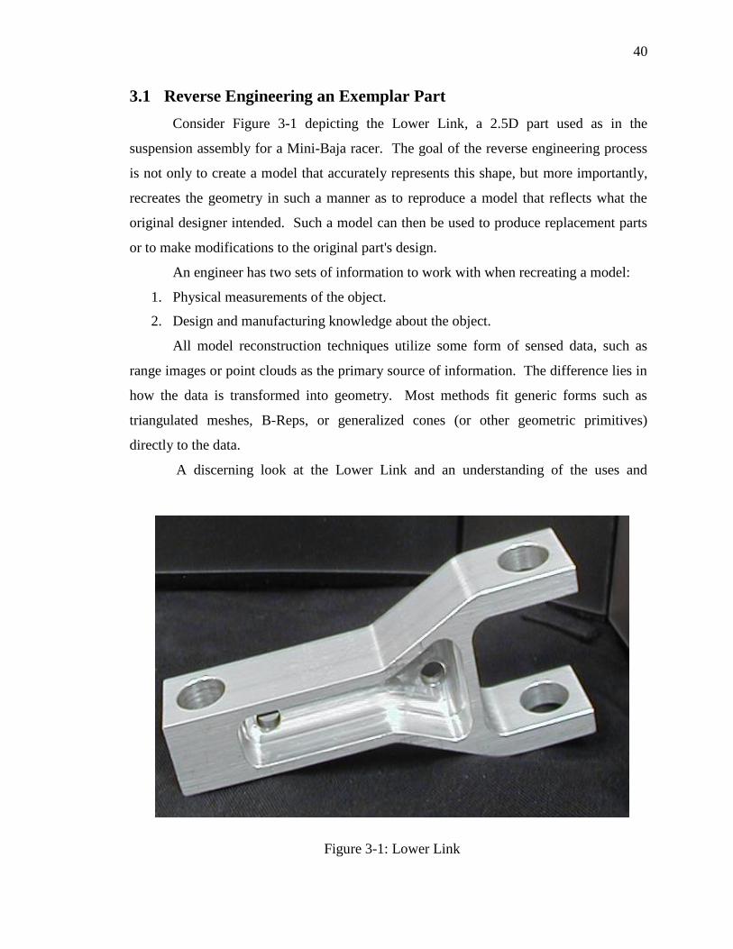
40
3.1 Reverse Engineering an Exemplar Part
Consider Figure 3-1 depicting the Lower Link, a 2.5D part used as in the
suspension assembly for a Mini-Baja racer. The goal of the reverse engineering process
is not only to create a model that accurately represents this shape, but more importantly,
recreates the geometry in such a manner as to reproduce a model that reflects what the
original designer intended. Such a model can then be used to produce replacement parts
or to make modifications to the original part's design.
An engineer has two sets of information to work with when recreating a model:
1. Physical measurements of the object.
2. Design and manufacturing knowledge about the object.
All model reconstruction techniques utilize some form of sensed data, such as
range images or point clouds as the primary source of information. The difference lies in
how the data is transformed into geometry. Most methods fit generic forms such as
triangulated meshes, B-Reps, or generalized cones (or other geometric primitives)
directly to the data.
A discerning look at the Lower Link and an understanding of the uses and
Figure 3-1: Lower Link

41
tolerances necessary for a valid manufacturable model belies the applicability of these
general forms and suggests that a structured, domain specific method is required.
Figure 3-2 represents the data cloud constructed by sensing the Lower Link.
Notice the general noise, the rounding of corners, and the systematic error in the pockets
(as seen by the sloped line in the third view). The average sensing error along the
exterior profile of the part (where the best data is collected) is approximately 130
microns. The worst case data points were over 900 microns off the surface. For data on
the interior pockets the average error is 300 microns and worst case is 1675 microns.
General fitting techniques cannot adequately compensate for these inaccuracies if the
resulting model is to be manufactured as a valid replacement for the original.
Algorithms exist that will automatically transform a data cloud into an irregular
triangulated mesh (Figure 3-3) forming a model that can be machined. This "fitting"
process can be applied directly to the data, and thus no knowledge of the object's function
is needed. Although the reconstructed mesh closely conforms to the data cloud, there is
no guarantee of topological equivalence with the original design; more importantly, while
each face of the mesh, on average, may be a good local approximation to the surface of
the original model, the combined elements of the mesh unduly fluctuate based on local
data inaccuracies, and thus form a poor representation of the true machined surfaces of
the object.
From this evidence it is asserted that knowledge about the design and manufacture
of a part is as important as the sensed data, which should be considered only one of
several associated sources of information used to generate a model. By analyzing
hypothesized geometry both in relation to the sensed data and based on knowledge of
how these types of parts are designed, manufactured, and assembled, a higher quality
model can be constructed. In Chapter 4, a focus is made on how this knowledge can be
formalized for use with general optimization techniques to fit both the data and the
functionality of the desired part simultaneously.

42
Figure 3-2: Views of the Lower Link Data Cloud

43
3.1.1 Local Constraints
Knowledge of the design process indicates that most, if not all, geometric
elements of a part are designed from simple well-defined shapes that serve specific
purposes. Expert engineers use this information to simplify the job of modeling a part.
By quantifying the possible design artifacts, an algorithmic fitting process can also be
greatly simplified, resulting in a more accurate reconstruction.
By applying knowledge of 2.5D manufacturing and design techniques, several
educated assumptions about the general geometry of the Lower Link can be made (i.e.,
Figure 3-3: Triangulated Mesh Representation (Lower Link)

44
the main "flat" surfaces are presumed to be planar, the curves appear to be continuous,
there are holes, profiles, and pockets in the part, etc.). By exploiting the fact that
arbitrary geometry is unlikely, more appropriate models can be developed for reverse
engineering. Owen [24] suggests a feature-based breakdown of 2.5D parts. Features
encapsulate the form and function of a part's geometry using a mathematical formalism
that constrains the possible configurations of a part. These well-defined geometric
primitives reduce the possible DOFs of the constructed model and force the geometry to
match a hypothesized version of the designed model. For example, they enforce a
smoothness quality16
between the arcs and line segments in the contours.
One of the important aspects about 2.5D features is that they represent a piece of
2D geometry that has been extruded into the third dimension. This realization allows a
two-tiered fitting process, beginning by extracting and fitting the bounding planes, and
then followed by a 2D fit of the profile curve data. To recreate the original surfaces,
these curves are then extruded normal to the bounding planes.17
Figure 3-4 depicts a feature-based decomposition of the Lower Link. The
features of interest include holes, profiles, and pockets (all contained within their
bounding planes). During the reverse engineering session, the engineer would identify
each contour and hole for segmentation and fitting.
Features inherently enforce certain low level geometric constraints. In design this
limits the set of constructed entities to those that are easily manufactured. In reverse
engineering, this has the affect of forcing the fitting process to produce geometry that is
likely to be seen in real world parts.
3.1.2 Global Constraints
The application of domain specific features is not in itself a panacea, as it is not
powerful l enough to fully exploit and capture all the functional properties of an object.
16 Specifically C1 continuity.
17 In practice the planes are fit to the data and then the segmented 3D data
representing the feature are projected onto one of the bounding planes. After the
feature is fit as a planar curve, it is projected back into 3D.

45
Figure 3-4: Feature-based Description

46
The reconstructed features should automatically be positioned in such a manner as to
recreate, as far as possible, the properties intended by the part's designer. Failure to do so
can result in a close approximation that still does not meet the tolerances required by the
reverse engineered model.
The limited ways in which primitives can be combined to form mechanical
features is in of itself a type of constraint on the possible geometry of an object.
Enforcing global geometric properties across a single feature or between multiple
features can augment these local constraints. For example, the designer has most likely
placed the two pockets (seen in the Lower Link) symmetrically. Likewise the walls of
the pocket have probably been placed in parallel to each other and the profile of the
object. If each pocket is fit separately, it is unlikely that they will end up symmetric to or
aligned with each other. Further, if each wall segment is fit separately, it is unlikely they
would end up truly parallel. If this were a high precision part, such a change in the center
of gravity could adversely affect wear and performance.
As another example, consider the upper holes on the Lower Link used to hold a
connecting pin. Current sensing processes result in poor data for holes because they self
occlude (especially small diameter holes) and have sharp discontinuities. If each hole is
fit independently, no guarantee can be made that the assembly will still function. Even a
small translation in the location of the center of high tolerance holes can prevent a mating
piece from sliding smoothly between them. In these cases, the importance of
constraining the centers of the holes and the common radii cannot be overstated. The
result of this process enforces that the functionality of the holes (holding a mating pin)
will be achieved, even if the sensed data contains error that would otherwise adversely
affect this property.
When attempting to model the Lower Link the reverse engineer would notice
several likely geometric properties (see Figure 3-5):
1. The 2.5D nature of the part suggests that the planar surfaces along the sweep
direction are all aligned.
2. The upper holes appear to be concentric and have the same diameter.
3. The outer profile edges help shape the interior pocket contour they surround.

47
Figure 3-5: Constrained Lower Link

48
4. The pockets on either side of the object look as though they contain identical
geometry offset along the part's sweep direction.
5. Many of the planar surfaces are parallel or perpendicular to each other.
A study of the Lower Link and similar parts makes it apparent that the geometry
in this domain is not free form, but highly structured. This structure can and should be
utilized during the model reconstruction phase. Constraints are a natural representation
for capturing knowledge of the design process. Table 3-1 contains a list of constraints
consistent with the design of 2.5D machined objects. These constraints represent
characteristics implicitly and explicitly utilized during part design.
3.1.3 Lower Link Conclusion
A key insight about the geometry of 2.5D machined parts is that most, if not all,
of elements are constrained externally by their neighboring features and internally by
their own design. The lower link is sensed initially as an unordered point cloud. To
create an appropriate model for manufacture and redesign, it is necessary to apply more
information than just the sensor data.
Table 3-1: Identified Constraints
Incidence Primitives (lines and arcs) meet at well-defined locations.
Smoothness Primitives meet with equivalent tangents.
Perpendicularity
Parallelism
Feature lines are often aligned parallel to each other or at right angle
intersections.
Concentricity The center of holes and arcs are often created to be concentric with
one another.
Symmetry Features are often created in whole or in part with symmetric
relationships around specific axis lines.
Common Angles Lines and planes often intersect at well-defined angles, such as 30, 60
or 90°.
Radius
Consistency
Arcs often have identical radii when compared with other arcs in the
contours of the object. Likewise, holes in an object are often drilled
with the same bit or a limited set of bits.
Width
Consistency
Pocket walls and other types of features often contain equivalent
thickness throughout the entire part.
Identical but
Offset
Certain geometries are found in one part of the object and repeated in
other areas.

49
Knowledge of the design and manufacturing process can help produce low DOF models
that can be further constrained by domain specific knowledge. The resulting models
more accurately represent the likely geometry of the part than those produced by
traditional fitting methods and contain topology that most likely matches that envisioned
by the original designer.
3.2 Design and Manufacturing in the Domain of
2.5D Axis Machining
This research claims that certain geometries are much more likely to be found in
the realm of 2.5D mechanical design because of the nature of such parts, and thus the
geometric properties of these shapes should be exploited when reverse engineering them.
To support this claim, the concepts of design practice, manufacturing knowledge, and
design intent will be briefly examined.
1. Manufacturing Knowledge: 2.5D parts are usually machined using a three axis
machining center. This machining process limits the possible geometry of a part. A
block of aluminum (or other material) is placed in the milling machine, at which point
a tool (i.e., end mill, drill, ream, tap, etc.) aligned with the Z-axis is used on the initial
stock.
Typically a part has a 2D contour that is swept into the third dimension.
Machining away all material on the outside of the contour physically reproduces
this. For holes, the drill bit completely pierces the stock, producing holes aligned
with the Z-axis. This machining process lends itself to extruded 2D geometry and
planar surfaces.18
In the cases where off-axis geometry is needed, the part must be removed from
the machine tool and then refixtured. This is usually accomplished by remounting
the part along another planar surface that has been machined flat by the previous
machining cycle. Such a surface is almost always orthogonal to the original
18 Three axis machining can be adapted to produce certain free form pseudo 3D
geometries, but this type of machining is seldom used in practice.

50
mounting surface. At this point, the same limitations of the three axis machining
center apply.
2. Design Intent: Design intent can be broken into two forms, feature interaction and
model appropriateness.
Feature interaction is the idea that the perceived interaction between features is by
"design" and not by coincidence. A simple example would be that if two walls of
a 2.5D part appear to be parallel, then it is likely they were intended to be parallel
and should be fit as such.
Designers often choose the simplest geometry to accomplish their goals. Model
appropriateness describes the ability of a model to represent this goal. This means
that the fit geometry is consistent with the designer's intent. Hence even if a high
DOF spline can better represent the sensed data for a certain feature, it would not
closely match the designer's conception of the feature.
3.3 The Advantages Attained by Using Constraints
The use of consistent patterns in the design of 2.5D manufactured parts provides
the foundation behind many design systems and the reverse engineering system presented
in this dissertation. Regardless of the design system (which differ in implementation and
representation) a designer uses, the results tend to be straightforward with well-defined
characteristics. Thus, whether a designer uses a system based on non-uniform rational B-
splines (NURBS), features, triangulated polygons, or even hand drawn lines, it does not
alter the fact that the resulting design contain the same properties which can be leveraged
during reverse engineering.
The power gained by using constraints is the ability to lower the DOFs of the
problem, making the system more likely to converge to the desired result and less
affected by noise. The following areas demonstrate how this advantage is realized: 1)
enforcing design intent, 2) simplifying the fitting process, and 3) binding geometry
together.

51
3.3.1 Enforce Design Intent
Design practice suggests that even complex models are often defined in terms of
simple well-defined shapes. With no constraints applied, standard modeling systems
allow the creation of many arbitrary shapes not seen in manufacturing. Even a simple
constraint that forces segments of a profile to be incident to each other is necessary to
enforce a real world property that is intuitive to the designer and reverse engineer. Thus
the use of constraints can limit the reverse engineered model to the realm of feasible
models produced by designers. This can be done in two manners. First, the choice of
primitives can provide a powerful tool. Second, mathematical constraints can be applied
over the primitives to further limit their DOFs.
3.3.2 Simplify the Fitting Process
The fitting process involves a weak search over a large vector of parameters. Any
step that can reduce the number of parameters or the size of the search space speeds the
search and reduces the effects of noise. Constraints can be used both for DOF reduction
and to set feasibility boundaries on the search.
3.3.3 Binding Geometry
Traditionally, physically separate geometric elements are fit independently. This
causes multiple fitting steps on smaller amounts of data and allows geometries that are
linked by the design to “float” unrelated to their counterparts in the reconstructed model.
When fitting the various geometries that make up an interesting part, it is common to find
that they share certain geometric properties. This is often the case, for example, where
several holes have the same radii or are concentric with each other, where the walls of a
pocket have a constant offset from their counterparts on the surrounding profile, or where
the diameter of a round is consistent throughout a model. Because of the errors
associated with data sensing (notably noise and missing data), significant parametric
errors can be introduced when fitting geometry. These problems can be addressed by the
use of geometry spanning constraints.
Binding geometry across a single part can reduce the possible forms of the part
and simply the fitting stage. Several examples were detailed using the Lower Link,

52
including symmetrical pockets and aligned holes. Other examples include common wall
thickness, symmetric halves of a part, and mating holes in an assembly. Binding
geometry across the multiple parts of an assembly can be instrumental in enforcing
tolerances and thus allowing assemblies of parts to fit with together.
3.4 Taxonomy of Constraints
When recreating a mathematical model of a manmade object from an exemplar
part, it is beneficial to provide mathematical constraints that enforce known or suspected
design artifacts. One way to achieve this is to use a limited set of features, with low
DOFs, for modeling aspects of a part. This ensures that the optimization process does not
fit just the noise inherent to sensed data, but also fits the inferred design intent of the
object. Unfortunately, even simple features and subfeatures are not restrictive enough for
the reverse engineering application. There is a need to further limit the possible
geometry of the model. This can be accomplished by applying certain geometric
constraints to the optimization process, limiting the feasible geometry of the part to those
that are common in the domain of interest.
The previous sections described constraints in terms of local and global
properties. This section presents a clarified taxonomy of constraints. Many 2.5D
manufactured parts can be formed by combining a small set of domain specific
primitives, termed features.19
Features form the basic building blocks of design,
representing such items as pockets, profiles, and holes. Features are composed of
geometric primitives, notably lines and arcs. The design process suggests these
primitives can only be combined in a few limited, well-defined ways. These composition
characteristics are termed design pragmatics. A further level of control, termed
functional constraints, governs the placement of features and subfeatures in relation to
each other.
19 From this point on, the term feature and domain specific primitive will be used
interchangeably. Any use of the term primitive (as opposed to domain specific
primitive) will refer to the line and arc geometry that make up the basic building
blocks of pockets and profiles.

53
Figure 3-6 symbolically depicts the increases in accuracy gained from adding
additional constraints and thus reducing the possible DOFs of the model.
3.4.1 Domain Specific Primitives
It has been shown by Thompson et al. [35] that features form a natural
decomposition of 2.5D manufactured parts. The use of domain specific primitives such
as those shown in Table 3-2 can greatly increase the accuracy and appropriateness of a
recreated model. Features are based on common design practices and facilitate making
simple accurate models. The fact that these features are used in design is a strong
argument for their use in reverse engineering.
Features, such as pockets, in terms of 2.5D architecture, are formed from the
combination of two bounding planes and a characterizing contour. Contours are formed
from a collection of ordered primitives that fully define the 2D geometry of the feature.
Without any limiting constraints these contours could contain arbitrary geometry. In
practice a number of pragmatics are enforced. These pragmatics will be discussed in the
following section.
Perhaps not as readily grasped is the idea that optimizing over features is simply
another form of constrained optimization. Features were created based on common
engineering structures, and thus map directly to design artifacts. For example, consider
Figure 3-7, which depicts three separate optimizations to the same set of data. The
piecewise linear interpolation produces zero error when compared to the data, but with
the knowledge that the data points were scanned from a circular hole, a better
representation can be chosen, constraining the fit to a circular shape.
A distinction is made between modeling error and data-fit error. Features help
decrease modeling error and thus increase the accuracy to the original design, but when
compared to the data, they increase the error over more general primitives.
Features also form natural decompositions of machined parts. They hypothesize
the general shape and are useful in segmenting the scanned data into local regions.
Further, features form a basis for applying global constraints across objects. This follows
from their algebraic descriptions. Such global constraints will be discussed in the section
on functional constraints.

54
Figure 3-6: Increased Accuracy
Table 3-2: Feature Taxonomy
Feature A high level geometric entity formed by combining subfeatures and
microfeatures.
Holes Blind, Through, Counter-sunk, Counter-bored, Tapped
Contours Pocket, Profile, Island, Boss
Slots
Primitives The geometric primitives used to form features.
Planes
Lines
Arcs
Micro
Features
A manufactured geometric entity that is too small to be accurately
identified by automated sensors.
Rounds Smooth exterior surface between meeting planes
Fillets Smooth interior surface between meeting planes
Accuracy
Additional Constraints/ Reduced
Degrees of Freedom
Functional
Constraints
Pragmatics
Primitives

55
Fit: Line Interpolation Oval Fit Circle Fit
Data Error: Zero Low High
Design Error: High Medium Low
Figure 3-7: Fit Options
Features are represented as tagged parameter vectors. At its most general, the
feature vector for the contour pocket seen in Figure 3-8 would be composed of the
following primitives:
Arc1, Line1, Arc2, Line2, Arc3, Line3, Arc4, Line4, Arc5, Line5, Arc6, Line6
The geometry of each primitive is represented as follows:
Arcs: Center(x, y), Radius, starting theta, ending theta
Lines: End 1 (x, y), End 2 (x, y)
An arc requires five values and a line segment requires four. The pocket profile is
defined by 54 values (six lines and six arcs). Fortunately a great deal of simplification
can be applied to these structures to reduce the number of parameters required to
represent this geometry.
3.4.2 Domain Specific Pragmatics
Mechanical features have many implied restrictions on their possible geometry.
Their representational power must be explicitly captured by the reverse engineering

56
system in order to force the reconstructed model into a form that is likely to recreate the
desired part. Primarily, only a limited set of primitives, as discussed above, is allowed to
represent each feature. Second, the primitives can only be placed based on a rigid set of
rules. These properties/restrictions are termed domain specific pragmatics and they
include:
Incidence - Connectivity of adjoining lines and arcs
Smoothness and Continuity - Arc features usually form smoothing actions
between line segments, providing C2 continuity
These pragmatics represent the intuitive idea behind how features are constructed
and manufactured. They further allow the reduction of the DOFs necessary to represent
features. Now line segments can be replaced with lines that require two DOFs to
Figure 3-8: Pocket Profile

57
represent (the normal and distance from the closest point on the line to the origin). Arcs
can be represented based on their surround geometry and as is described in the next
chapter, require as few as one DOF. Pragmatics represent the implicit assumptions made
by designers (and reverse engineers) when creating models.
3.4.3 Functional Constraints
Domain specific primitives model the recreated geometry in a manner similar to
that of the design process. For 2.5D machined parts an appropriate choice of primitive is
that of design feature. Domain specific pragmatics enforce even greater restrictions on
the possible geometry of the features. For example, a domain specific pragmatic forces
the use of continuous smooth contours. Functional constraints attempt to enforce high-
level design intent.
When an engineer designs a part and chooses a specific feature, it is with the
expectation of a certain functionality. An example would be the placement of symmetric
weight reduction pockets to ensure a correct center of mass, or the placement of
concentric holes to ensure the acceptance of a mating feature. With the error inherent in
data scanning, small variations are likely to corrupt the recreated model. These variations
can impact the usefulness of the replacement items.
Once again consider the Lower Link example in Figure 3-1. The line primitives
that make up the profiles and pockets were not randomly placed but were purposely set at
parallel and perpendicular angles to each other. Further, the top and bottom pockets as a
whole were set directly opposite from each other and centered in the overall profile. The
top and bottom mating holes were machined to accept similar connectors and thus are of
the same radii.
All of these properties are designed into the object to promote its functionality,
while maintaining an easily machined geometry. By enforcing these constraints, the
DOFs of the hypothesized model are reduced and each separate feature is bound to the
whole in a well-defined and enforceable manner.
This dissertation considers the effects of the following functional constrains:
Perpendicularity, Parallelism, Concentricity, Symmetry, Known Angle between

58
subfeatures, Arc Distance, Radius Consistency, Width Consistency, and Identical but
Offset features.
3.5 Overview
Figure 3-9 demonstrates the progression of constraints used to guide the
optimization of the bottom of one of the Lower Link pockets. As more information (in
the form of constraints) is applied to the reconstruction problem, the less unintended-
effects from sensor noise will bias the new model. In the following chapter the methods
for representing these features and constraints will be discussed.

59
Figure 3-9: Constraint Progression
General
Spline Fit
Feature
Primitives
Feature
Pragmatics
Local and Global
Functional Constraints
Parallelism
Wall Width Equality
Perpendicularity
Line and
Arc Fits
Continuity and
Incidence

CHAPTER 4
4 CONSTRAINT FORMULATION FOR MODEL
OPTIMIZATION
This dissertation claims that domain specific knowledge can be applied to the
model creation process to generate higher quality models. In the previous chapters, the
type of model and the properties inherent to the domain of 2.5D manufacture are detailed.
This chapter describes the formulation of both the model and the constraints in such a
manner as to be incorporated into an optimization algorithm. While this dissertation does
not attempt to advance the core field of optimization research, it shows the ability to
introduce domain specific knowledge via constraints into an optimization framework.
Each model is reconstructed based on a set of manufacturing features similar to
those utilized in feature-based design. Holes are defined directly by their parametric
geometry. Higher order features, such as pockets and profile-contours, are made up of
low-level geometric primitives (arcs and lines). Each primitive has one or more
parametric forms that can be used to construct the geometric form. These constructions20
are made based on the current parametric representation, the actual parametric values,
and ruler and compass composition algorithms.
All information necessary to construct the complete 2.5D geometry of the model
is kept in a feature vector. A feature vector is defined as the list of all parametric values
and topological information required to instantiate the model. The parametric values in
20 The term constructive geometry is used here to describe the transformation from
parametric space to geometric space using basic geometric rules (hence the term
ruler and compass). Various parametric representations can be used to define a
single geometric shape. For example, a line can be represented as a point and a
normal, or as an angle and minimum distance from the origin.

61
the feature vector are the components that define the optimization space. The topological
information contains which parameterizations are in use, as well as other book keeping
information necessary to reconstructing the model from a minimum set of parameters.
By adaptively changing the parametric values, variations of the shape of the object can be
hypothesized and tested.
The initial feature vector for a part is constructed via an interactive system that
fits low level geometry to the data cloud using standard least-squares fitting techniques.
These initial fits of the low level primitives (circles, lines, and arcs) form the input to the
constraint-based optimization process. First, the primitives are mapped onto features by
enforcing the appropriate domain specific pragmatics. Then higher-level functional
constraints are hypothesized from the low level geometry. Finally, penalty functions are
asserted and the optimization begins.
The process of enforcing smoothness and incidence on the primitives is
accomplished by intersecting adjacent lines and changing the radii of the arcs so as to
merge with adjoining arcs or lines. This produces small deformations in the feature that
are incongruent (as would be expected) with the sensed data. Under feature-based
reverse engineering, an optimization would then take place on each separate feature,
resulting in the final model. For the purposes of constrained optimization, the feature
vector, representing the entire model, is optimized, accentuating or alleviating these
deformations from the data to create a globally more appropriate and accurate model.
Once the initial model has been created, constraints are hypothesized and asserted
producing a new feature vector representing the same geometry but with a greatly
reduced number of parameters. Any constraints that cannot be directly represented
through a parameter-set transformation are used to construct penalty functions to direct
the optimization process. The output of this process is an instantiated parameter vector
that most accurately (to the criteria of the constraints and sensed data) represents the form
and function of the hypothesized original design.
4.1 Problem Formulation
The goal of the optimization process is to find the set of parametric values that
produce the model that best fits the actual 3D position data while concurrently preserving

62
the constraints asserted upon the possible geometry of the model. This problem can be
formulated as seen in Table 4-1. P represents the vector of parameters defining the
model geometry. M is a function that computes the geometric model based on the
parameters P. M contains algorithms for transforming from the parametric space to the
geometric space for each supported feature. T is a transformation function on p that
commutes geometric constraints into a reduced set of parameters, pr which is
constructively equivalent21
to the original, in that it can reproduce the same geometry as
produced by M(p). D represents the error between the constructed model and the data
points. E represents the violation of the constraints associated with the optimization. The
goal of the optimization process is to minimize F, the weighted sum: D + α * E.
By defining these functions, the reverse engineering problem is transformed into
an constrained optimization problem. The optimization is achieved by standard
methods,22
which, when applied to the parameter vector, pr produce the best model based
on the error criteria.
This research has successfully met the following objectives:
1. The model creation function M was designed incorporating a representative set of
2.5D feature geometry. The function was implemented using constructive ruler
and compass algorithms similar to those used in feature-based design packages.
2. The transformation function T was defined to reparameterize the model based on
the constraints, reducing the number of DOFs while maintaining the same
geometric representation. This function uses symbolic substitution methods and
has an understanding of the geometry creation methods found in M.
21 T also produces the book keeping information necessary for the transformation,
such as the current parameterization used by each feature. Because this
information is constant, it is not considered as part of the search space.
22 For purposes of this work, both Simplex Search (amoeba) and Powell’s method
(conjugate directions) were investigated. Both methods were amenable to the
formulation of the model and constraints used in this research and were able to
converge to acceptable minimums.

63
3. The function D, which computes RMS error between the sensed data set and the
current model geometry, was created. D also resegments the data during the
optimization in order to limit the effects of outliers on the optimization.
4. A method was created for producing E directly from the list of constraints. This
set of penalty functions was integrated into the objective function based on both
geometric properties (e.g., distance between two lines) and parametric properties
(e.g., radius equivalence).
Table 4-1: Problem Formulation
b: Global book keeping information necessary for the reconstruction of
the model.
C: The constraints asserted on the model.
D: The sensor data associated with the exemplar under reconstruction.
P: Vector of parametric values used to instantiate the model geometry.
Pr: A reduced DOF vector representing the same information as p based
on the asserted constraints and B.
M(p,b): A model creation function that constructs the physical geometry of
the model from a parametric list of values and types.
T(p,c)=Pr: A transformation function which reduces the number of parameters
based on the constraint list c.
D(M(Pr,b),d): D is an error function that computes the distance from d to the
model. (More precisely, this function must segment d based on the
distance to the closet primitive and then compute the RMS error by
summing the error over each primitive.)
E(M(Pr,b),c): Error derived from the violation of constraints, c.
F: The object function to be optimized over. Equivalent to D + α * E.
Alpha is a weighting term equalizing the data and penalty errors.
The optimization algorithm.

64
The application of T to create the new parameterization vector is a
preoptimization step that significantly reduces the complexity of the model under
consideration, and thus the optimization process itself. E is computed during each step of
the optimization based on constrained optimization techniques.
4.2 Constraint Representation
Features were introduced and formulated in Chapter 3. Consider a pocket feature
comprised of a bounding plane, an extrusion depth, and a contour. The contour is an
annotated ordered list of geometric primitives (viz., arc and line segments). Each part of
the feature is defined by its parametric values which, when instantiated, determine the
physical shape of the object. Under this formulation, many of the geometric constraints
can be applied over the parametric representation.
The first application of constraints is to reduce the number of parameters
necessary to define the model. T(p,c) = pr. This is accomplished by replacing multiple
parameters with a single parameter and a constructive method for recreating the lost
parameters. The reasons for reducing the number of variables are:
The constraints are implicitly enforced,
the optimization convergence is faster,
and the resistance to data noise is improved.
In the terminology of optimization, an interior point method has been created
which searches for the best possible (lowest error) model while maintaining all
constraints at each iteration of the optimization routine.
Because M constructs the physical geometry of the part based on ruler and
compass techniques, and because different parameterizations can be used to represent the
same geometry, it is not always possible to directly assert model constraints based on the
parametric representation. In this case, the constraints are used to explicitly guide the
optimization process by increasing the value of the objective function by an amount
related to the degree with which each constraint has been violated. Function E(M(pr),c)
is defined to calculate this result. Penalty functions force the optimization process to
converge on a model with the desired topology. This is equivalent to an exterior point

65
method, initially allowing infeasible configurations but then forcing the final
configuration towards a feasible model.
4.3 Construction of Primitives
The low level elements that make up the 2D geometry are arc segments, line
segments, and circles. For contours, domain specific pragmatics have shown that the
geometry of the primitives is locally restricted by their neighboring geometry, and thus
line segments can be represented as true lines, and arc segments can be represented as the
curving action between lines. Primitive construction is the technique that constructively
builds the physical geometry from the reduced DOF representations using ruler and
compass techniques.
For example, consider two line segments that meet at a corner. If each line
segment keeps track of the common endpoint, consistency errors can occur. If, instead,
both line segments are transformed into line representation, then the common point can
be calculated by intersecting the two lines. In this case, each time the parameterization of
either line changes, the new end-point must be recalculated. For the constructive
techniques involved in the features defined in the 2.5D domain, the complexity of the
operation is constant.
Now, consider a circular arc bounded by two lines. As arcs are smoothing actions
between two line segments, the arc must be incident and tangent to the neighboring lines.
Therefore the arc can be constructed based on the line position simply by knowing its
radius. Figure 4-1 represents the constructive geometry transforming the parametric
representation into the geometric representation. The point I represents the intersection
of the two bounding lines. By adding the normalized bisector vector times the distance d
to the point I, the new arc center is determined. The intersection points between the lines
and the arc are then determined by projecting the center onto both lines. This provides
the complete geometric form of the line-arc-line structure.
In most constructive geometric operations, care must be taken to deal with
singularities, such as if the lines become parallel in the line-arc-line example. In such a
case, multiple constructive forms may be necessary and a transformation between them
established. Alternatively, if the singularity can be hypothesized before the optimization

66
Figure 4-1: Arc Construction Based on Radius
(again as in identifying the parallel nature of the constraining lines) then only the parallel
formulation need be used.
Another interesting feature found in the 2.5D domain is that of the boss, or triple
arc subfeature (Figure 4-2). A boss often forms a strengthening structure around holes.
It is composed of three arcs with C1 continuity. The radii of the outside arcs are equal,
and the whole structure is symmetric based on the surrounding lines. Several
parameterizations of this feature are required based on whether the bounding lines
intersect, are parallel, or are collinear. This subfeature is an example of a domain specific
structure that requires deep understanding of the domain, yet yields large dividends in the
reconstruction process.
Line 2
r r
d
Line 1
I θ
Arc Center
Lines Bisector Vector
d = sin(θ) / r
Arc Center = I + (Line
Bisector Vector * d)

67
Figure 4-2: Boss (Triple-Arc) Subfeature
It should be noted that as the DOFs are reduced certain book keeping measures
must be made, such as retaining the symbolic topological information (Line followed by
an Arc, followed by a Line, etc.). In the case of the line-arc-line structure, there are four
possible quadrants where the arc could fall based purely on the intersection of the lines.
It is therefore necessary to store which quadrant represents the interior of the object. This
allows the model construction method to recombine the reduced parameter model back
into the full geometry of the part. This information is considered static throughout the
entire optimization process and is not considered a DOF.
4.4 Defining the Reduced Degrees of Freedom Model
By using the asserted constraints on the geometry to produce the reduced
parameter vector a powerful technique for constrained optimization is developed. The
phrase DOF reduction is used for this technique. Two methods have been identified for
reducing the DOFs of a model: symbolic substitution and feature re-parameterization.
4.4.1 Symbolic Substitution
As the name implies, symbolic substitution replaces equivalent symbolic
parametric variables with a single common variable. Symbolic substitution is valid when
primitives have parameters representing identical information, such as the radius of a
hole, or the angle of a line.
Consider the two lines L1 and L2, defined by an angle, q, representing the line's
normal direction, and the distance, d, representing the shortest distance from the line to
r1
r2
r1

68
the origin. If the lines are parallel, then this angle parameter can be redefined in terms of
a single angle. Thus given:
Line1 (d1, q1) &
Line2 (d2, q2)
and the constraint:
Parallelism (q1 == q2)
a new description is generated:
Line1 (d1, q1) &
Line2 (d2, q1)
The result is a four-DOF problem being reduced to a three-DOF problem. For
holes, defined by a center and a radius, symbolic substitution is possible for concentricity
constraints.
Hole1 (x1, y1, r1) &
Hole2 (x2, y2, r2)
The constraint:
Concentricity (x1, y1) == (x2, y2)
The result:
Hole1 (x1, y1, r1) &
Hole2 (x1, y1, r2)

69
Thus a six-DOF problem is reduced to four. Likewise, for radius equivalence
constraints, the single radius parameter can be substituted among all common radii holes,
reducing the number of parameters necessary to represent each additional hole by one.
4.4.2 Feature Reparameterization
Unfortunately, symbolic substitution only works when two or more primitives
have corresponding parameterizations (and thus construction methods). Consider a hole,
represented by (x,y,r) and a bounding boss. A concentricity constraint cannot be directly
applied because there is no direct representation for the center of the middle arc.
To address this shortcoming, it is noted that many geometrical forms can be
parameterized in multiple way and still be instantiated to the same physical geometry. A
line can be described as "Ax + By + C = 0" or as "y = mx + b" or as "(d1, q1)." Feature
reparameterization is the modification of the representation of a primitive, giving it a new
parameterization that can then be used for symbolic substitution.
The physical geometry for a linear edge on a model is represented by the line
segment (x1,y1), (x2,y2). The slope of the line is not directly represented by this
parameterization. By transforming the line segment into a line, the angle becomes
available:
Line Segment(x1,y1), (x2,y2) Line(d1, q1).
At the same time the end points of the line are no longer directly available and
must be computed by some new method (usually the intersection of the current line with
the next line in the contour).
The choice of reductions is not arbitrary. In the arc example above, rather than
calculate the start and end theta values for the arc segment by projecting the center of the
arc onto the neighboring lines, the lines could be computed based on the angle of arc
segment end-points. This formulation is poor because small fluctuations in these angles,
which would be likely to occur because of segmentation errors, would cause large

70
fluctuations in the line normals and would not necessarily maintain other line constraints
such as parallelism.
For this work, the following ordering of primitives was used to decide which
primitive required a new parameterization: lines, single arcs, holes, and triple arc
features. Because of the general stability of the line parameterization and the widespread
use of lines in this domain, most structures were based on the surrounding linear
structure. When concentric holes and arcs occur, the hole parameterization is based on
reconstructing the arc first and then equating the arc center to the hole center.
The result of symbolic substitution, feature reparameterization, and subfeature
construction is the ability to apply the model definition function M on a set of fewer
parameters while still producing a physical model equivalent to the initial model. The
advantages of reducing the number of variables necessary to represent the geometry
cannot be overstated and include superior noise resistance, more tractable problems, and
faster and more accurate convergence.
4.5 The Optimization Function
Once the DOF reduction has taken place, the optimization process commences.
All the constraints that cannot be symbolically reduced are imposed in terms of penalty
functions during the optimization process. The objective function, F, is the weighted sum
of D and E. The optimization can be defined as finding:
)))),,(()),,((min(( cbpMEdbpMD rr
D calculates the sum of the square of the distances from each sensed data point to
the appropriate primitive in the model. E calculates the violation of any constraints that
have not already been symbolically formulated and represents the summation of the set of
penalty functions. As described in the Chapter 2, penalty functions limit the feasible
region of the optimization surface.
The following examples show the penalty functions used for concentricity and
parallelism, where pi represents the center point of each hole, and vi represents the normal
to each plane:

71
Concentricity: ƒ(p1,p2) = (geometric distance from p1 to p2)2 * ki * wi
Parallelism: ƒ(v1, v2) = | 1 - (v1· v2) | * kj * wj
where ki and kj are the controlling parameters and wi and wj are scaling parameters. The
strength (magnitude of the value) of the controlling parameters is gradually increased
during the optimization process to avoid initially falling into unrecoverable local minima,
while gradually forcing the geometry into feasible regions as the optimization converges.
A difficulty found with penalty functions is normalizing them so that the error
produced by one sort of constraint (say an angle based constraint) does not fade into
insignificance or completely overpower a second constraint (say a distance criterion).
The purpose of the scaling parameters is to adjust the value of each constraint into a level
commensurate with the order of magnitude of the error function and with the other
penalty functions. In this work, the penalty functions calculated scalar offsets
(concentricity, width equivalence, radii equivalence, etc.). Thus the scaling between
penalty functions was linear. The controlling factor of the penalty functions was
increased incrementally over four separate runs of the optimization. The final value was
three orders of magnitude greater than the initial value, forcing alignment errors of less
than 0.1 microns.
4.6 DOF Reduction Example
Consider Figure 4-3, which depicts a simple part called the Steering Arm. The
entire 2.5D geometry consists of two holes and an exterior profile containing five line
segments and three arcs. To create the physical geometry for this object the following
information is needed: for each line, the start and end points; for each arc, the center, the
radius, and the start and end thetas; for the holes, the center and the radii. Specifically,
the following geometric values are needed:

72
Line1: Start(x,y), End(x,y)
Arc1: Center(x,y), Radius, ThetaA, ThetaB
Line2: Start(x,y), End(x,y)
Arc2: Center(x,y), Radius, ThetaA, ThetaB
Line3: Start(x,y), End(x,y)
Line4: Start(x,y), End(x,y)
Arc3: Center(x,y), Radius, ThetaA, ThetaB
Line5 Start(x,y), End(x,y)
Tie Rod Hole: Center(x,y), Radius
Mounting Hole: Center(x,y), Radius
The above describes the geometry of the pocket in its most complete form and
requires 41 DOFs. The following constraints are asserted on this geometry: The profile
primitives are incident and continuous, the tie rod hole is concentric to the large profile
arc, lines two and five are parallel, lines one and two are perpendicular, and the
mounting hole is centered in the stock. The remainder of this section describes the
transformation from this low level geometry to a feature vector utilizing a reduced
parameter set that is still capable of constructing the geometry.
The first goal is to enforce incidence and continuity, reducing the number of
parameters in the process. As detailed earlier, the arcs can be described as smoothing
Figure 4-3: Steering Arm

73
actions applied to the intersection of the lines. Therefore, the line segments can be
redefined as lines (using an angle/distance representation) bounded by the arc segments:
Line1: Theta1, Distance1
Line2: Theta2, Distance2
Line3: Theta3, Distance3
Line4: Theta4, Distance4
Line5: Theta5, Distance5
The constraint hypothesis step23
asserts lines two and five as parallel to each other
and perpendicular to line one. This allows the following symbolic substitution:
Line1: Theta2 + 90°, Distance1
Line2: Theta2, Distance2
Line5: Theta2, Distance3
Each arc can now be defined based on its radius and neighboring lines and the
geometry constructed via the a fore mentioned ruler and compass method. This reduces
the basic geometrical description of each arc from five DOFs to a constructive
description requiring one DOF and insuring C1 continuity:
Arc1: Radius1, Line2, Line3
Arc2: Radius2, Line3, Line4
Arc3: Radius3, Line4, Line5
The final hypothesized constraint is that the tie rod hole and arc two are
concentric represented by the following substitution:
Arc2: Radius2, Line3, Line4
Tie Rod Hole: Center of Arc2, Radius4
Using incidence, smoothness, parallelism, perpendicularity, and concentricity
constraints, the DOFs of the Steering Arm has been reduced from 41 to 15. By
instantiating these parameters, the Steering Arm's geometry can be regenerated with these
constraints implicitly retained. The final requirement is that the mounting hole must be
located equidistant to Line2 and Line5.
23 The next chapter details a strategy for automatically generating the appropriate
constraints. For the purposes of this example, the engineer asserted the
constraints.

74
4.7 Penalty Function Example
Due to small errors in the manufacture and/or the error associated with the
scanning process, it is unlikely that the recreated mounting hole will end up exactly
centered in the Steering Arm profile. A reasonable inspection of the part would suggest
that this property was very likely to exist in the original design. To remedy this situation
a constraint is asserted stating that the center of the hole is equidistant to the walls of the
profile.
Consider the formulation of Line2, Line5, and the mounting hole from the
Steering Arm.
Line2: theta2, distance2
Line5: theta2, distance2
Mounting Hole: center(x,y) and radius
There is no direct correspondence between the geometry or parametric
representations of these features. Therefore it is necessary to construct a penalty function
to account for this constraint. The error function of interest becomes the difference in
distance from the center of the hole to the lines.
(Distance(line2, center) - Distance(line5, center))2 * kj * wj.
During each iteration of the optimization process, this value is calculated and
added to the error value associated with the current iteration. As wj is gradually
increased the center of the hole is forced closer and closer to the center of the two lines.
4.8 Discussion of Under and Over
Constrained Geometry
In the case of constraint-based geometric construction systems (i.e., solvers), a
large effort is made to deal with the problem of over and under constrained geometry.
Under constraining implies that not enough information is present to fully describe the
geometry of the object. Over constraining implies that more constraints are asserted on

75
the geometry than are physically possible to maintain.24
In the reverse engineering
setting, these problems are not of the same concern for the simple reason that a real world
instantiation of the geometry already exists.
First of all, a distinction must be made between the constraints imposed over the
geometry on the model, and the "constraint" which is the sensed data itself. The tools for
creating the initial feature vector only allow geometry that has a physical representation.
Therefore the initial geometry can be considered well constrained.
Because the geometry of the part is well defined before the constraint
optimization process and at least some data points are available for all primitives of the
part, it is impossible to under constrain the reverse engineering system. The geometry is
in fact always constrained by the physical data when no higher-level constraints are
asserted.
The only concern is when the system (or user) provides a set of assertions on the
geometry which create an over constrained set. In the case of symbolic substitution, the
last substitution to be made will overrule previous substitutions. This results in utilizing
one constraint and removing another. In most cases where this happens, the physical
geometry of the recreated model is obviously inconsistent with the data, thus quickly
allowing the engineer to identify the illegal constraint and remove it.
In the case of constraints represented by penalty functions, the numerical methods
will attempt to minimize the error, resulting in an averaging of the inconsistencies.
Again, this should be immediately apparent to the engineer via physical inspection of the
recreated model and analysis of the final RMS error associated with each feature.
In summary, over and under constrained geometry is a difficult problem in the
area of geometric solvers, but because a physical instance of the part exists for the reverse
engineering process, it is not possible to under constrain the problem, and an over
constraining of the problem results in immediate and apparent discrepancies in the
topology of the model and the error associated with the features representing the model.
24 An over constrained set of assertions, which can be reduced to a well-constrained
set because one or more constraints are interdependent, is not considered over
constrained.

76
4.9 Constraint Formulation Summary
Constraints are formulated directly on the parametric representation of the
geometry either by appropriate substitution or by penalty function creation. Table 4-2
lists the identified constraints and their reformulation for use with the optimization
process.

77
Table 4-2: Local and Global Constraints
Incidence
Line to Line Intersection forming corner.
Line to Arc Projection of arc center onto line to form arc segment end point.
Arc to Arc Any case of arc to arc incidence is handled by special
constructive subfeatures, such as a boss.
Smoothness
Line to Arc Arcs are formulated as smoothing actions on lines based on the
radius of the arc.
Arc to Arc As above (arc to arc).
Perpendicularity
Line / Line The angular value of the first line is symbolically substituted for
the second line (the value is then adjusted 90°)
Parallelism
Line / Line The angular value of the first line is substituted for the second
line.
Concentricity
Arc / Arc A Penalty function is constructed based on the calculated
distance between the two centers.
Arc / Hole The arc center is substituted for that of the hole.
Symmetry - Symmetry is achieved by a combination of penalty functions and
other constraints.
Radius Consistency
Arc / Arc The radius of one arc is substituted for the next.
Arc / Hole The radius of the arc is substituted for the hole.
Width Consistency
Lines / Lines A Penalty function is calculated based on the square of the
distance between the first set of lines minus the distance between
the second set of lines.

CHAPTER 5
5 AUTOMATIC CONSTRAINT ACQUISITION
The advantages of and methods for applying constraints during the fitting process
have already been discussed. The assumption has been that the constraints are known a
priori to the global optimization phase, and that these constraints are accurate and
meaningful. The important question remains: How were these constraints identified?
Manufacturing and design knowledge implies not only how certain constraints should be
enforced mathematically, but also which constraints are likely in the domain of 2.5D
manufactured parts. This knowledge provides two insights. First, a well-defined list of
possible constraints over each feature (or its associated primitives) can be identified.
Second, a test for likely constraints can be implemented based on approximate equal
parametric values determined during the initial fittings. Below is a list of the steps
employed by Owen et al. [24].
1. Scan part to produce data cloud.
2. Manually segment bounding plane data and then fit individual plane.
3. Manually segment single feature data.
4. Fit data to lines and arcs based on local feature constraints.
5. Repeat steps 2-4 until all features have been identified.
6. Build model on a feature-by-feature basis.
These steps are augmented as shown below. Step five is the subject of this
chapter, and steps six and seven are the subjects of the previous chapters.
1. Automatically segment and fit bounding planes.
2. Constrain the bounding planes based on alignment constraints.
3. Semi-automatically segment and fit features.
4. Identify likely constraints.
5. Build optimization function over all features enforcing constraints.

79
6. Optimize over all features simultaneously while maintaining constraints.
5.1 Manufacturing and Design Knowledge
Manufacturing and design knowledge can be used to formulate likely constraints
that can apply to the specific features in a domain. As detailed in Chapter 3, certain
geometric topologies and relationships are implicitly and explicitly used in the design and
manufacturing of the 2.5D parts considered here. Some of these qualities are enforced
during the reverse engineering process by the use of features that mimic the design
patterns of the object. Other properties must be explicitly denoted by the reverse
engineering system.
The first application of constraint acquisition is based on the implied qualities of
three axis machining. In the case of these parts, the planar faces bounding an extruded
2D curve are almost always parallel to one another. This quality is implicit both in the
designers sketch and in the CAD representation. During the reverse engineering process,
a decision must be made on how to handle this and similar situations.
Consider a pocket bounded by bottom and top planes. Previous methods have
either fit both planes individually or only used one plane as the basis for the feature. This
leads to problems in calculating the height of the pocket as well as problems projecting
the data into two dimensions for fitting. Manufacturing and design knowledge promotes
the idea that the top and bottom planes should be fitted simultaneously with equivalent
normals. This results in parallel planes. Further, in the case where one bounding plane
is more accurately sensed (due to larger surface area or less occlusion) the optimization
function can be weighted to constrain the less accurate section of data to the more
accurate section. The result is a well formed bounding region for the feature of interest.
Additionally, problems arise when multiple features share the same bounding
planes. If it were the case that only data points near the feature were used for fitting the
bounding plane, or that the bounding plane was fit several times with different
segmentations of data, then multiple planes would most likely be introduced into the new
model where only one true plane existed before. High-level knowledge requires all
shared bounding planes be fit simultaneously with all hypothesized parametric
equivalencies enforced.

80
5.2 Parametric Equivalence
Parametric approximate equivalence is a method for identifying constraints on a
specific model. Given two primitives (fit directly based on the sensed data), of types α
and β, a cross reference is made to a correspondence table denoting the possible
constraints which can hold between the given types of geometry (See Table 5-1).
In the case of two holes, the centers can be concentric, or the radii can be
equivalent. In the case of two lines, the normals can be parallel or perpendicular, or in
the case of parallel lines, they can have a common distance from another line. For every
set of two primitives, the possible constraints are checked and a parametric equivalence
test is made. This test takes the form of a distance check for concentricity, a length test
for radii, or a theta check for parallel and perpendicular constraints:
Concentric Test: ||center1 – center2|| < δ1
Parallel test: |theta1 – theta2| < δ2
Perpendicular test: |theta1 – theta2| - 90 < δ3.
If a primitive is found to have a parametric value closely matching another
primitive, then a constraint is hypothesized suggesting that any error between the two was
caused by noise in the sensing process and a constraint needs to be enforced during the
optimization.
Parametric equivalence is a powerful tool for speculating on likely constraints.
These tests are valid because they are based on knowledge of logical design practices.
For example, a typical part with holes will have a minimum number of different radii. In
the case of threaded holes, the screws for one hole are quite likely to fit another hole.
Table 5-1: Example Constraints
Hole Line Arc Plane
Hole Concentric
Diameter Equiv.
Distance to Center of Hole Concentric -
Line - Parallel
Perpendicular
Distance to Line
- -
Arc - - Concentric
Radius Equivalence
-
Plane - - - Parallel
Perpendicular

81
Further, the radii of these holes are likely to be one of a set number of well-known drill
bit sizes.
Consider Figure 5-1 depicting both a profile and a pocket feature. The values in
Table 5-2 and Table 5-3 were computed fitting each separate primitive to its individual
segmented data. The lines are parameterized in terms of their normal and distance from
the origin. The arcs are parameterized based on their center and radius. By cross-
referencing every primitive, several relations can be observed.
Figure 5-1: Lower Link Profile and Pocket Features

82
Table 5-2: Lower Link Lines Parametric Values
Lines Normal in Degrees Distance from Origin
L1 3.135 2.636
L2 1.566 -0.548
L3 1.107 -0.443
L4 1.565 -1.172
L5 3.140 -2.612
L6 1.563 -0.843
L7 3.136 -1.239
L8 1.566 0.752
L9 3.142 -2.620
L10 1.564 1.078
L11 2.029 0.351
L12 1.565 0.451
L13 3.122 1.759
L14 1.563 -0.402
L15 1.106 -0.300
L16 3.133 -1.077
L17 2.026 0.191
L18 1.566 0.288

83
Table 5-3: Lower Link Arcs Parametric Values
Arcs Center (x) Center (y) Radius
A1 -0.020 -1.131 0.583
A2 1.507 -0.575 0.604
A3 1.504 -0.585 0.269
A4 1.521 0.469 0.280
A5 1.523 0.458 .610
A6 -0.007 1.025 0.571
A7 -1.536 -0.170 0.220
A8 -1.550 0.088 0.208
A9 0.034 0.807 0.519
A10 0.862 0.397 0.212
A11 0.858 -0.527 0.215
A12 -0.001 -1.014 0.607
First, lines L1, L5, L7, L9, L13, and L16 have normal orientations within 0.02
degrees. Likewise, lines L2, L4, L6, L8, L10, L12, L14, and L18 have similar
orientations, as do lines L3 and L15, and lines L11 and L17. As these values are very
close, they are automatically flagged as likely parallel constraints. Further, lines L5 and
L9 have similar normals and distance parameters, implying that they are in fact two line
segments on the same geometric line.
In addition to the parallel constraints, it is numerically apparent that many of these
lines have normals perpendicular to each other within a very small error delta. Thus
many of the lines, such as L1 and L2, can be flagged denoting a perpendicular constraint.
The same process is applied comparing the radii of each arc. The result is the flagging of
A7, A8, A10, and A11 as likely radius equal constraints.
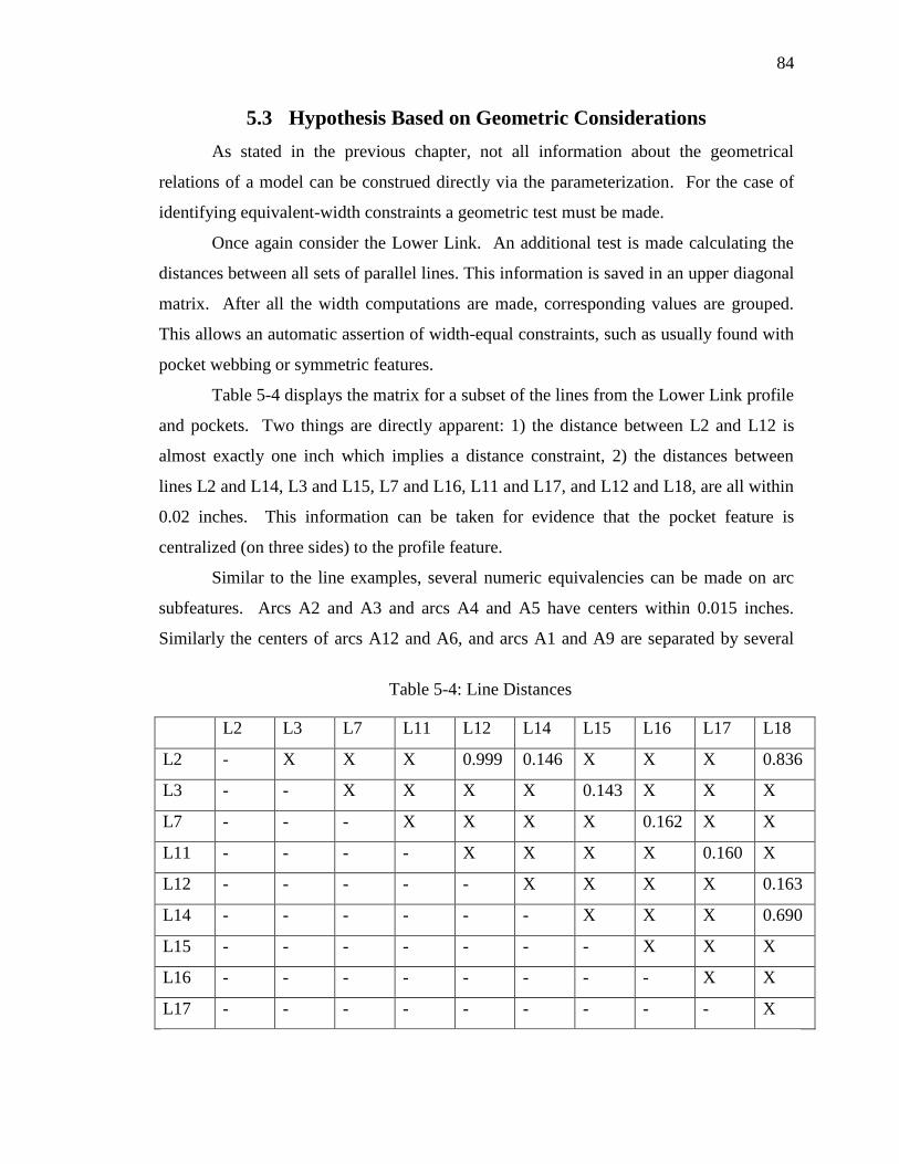
84
5.3 Hypothesis Based on Geometric Considerations
As stated in the previous chapter, not all information about the geometrical
relations of a model can be construed directly via the parameterization. For the case of
identifying equivalent-width constraints a geometric test must be made.
Once again consider the Lower Link. An additional test is made calculating the
distances between all sets of parallel lines. This information is saved in an upper diagonal
matrix. After all the width computations are made, corresponding values are grouped.
This allows an automatic assertion of width-equal constraints, such as usually found with
pocket webbing or symmetric features.
Table 5-4 displays the matrix for a subset of the lines from the Lower Link profile
and pockets. Two things are directly apparent: 1) the distance between L2 and L12 is
almost exactly one inch which implies a distance constraint, 2) the distances between
lines L2 and L14, L3 and L15, L7 and L16, L11 and L17, and L12 and L18, are all within
0.02 inches. This information can be taken for evidence that the pocket feature is
centralized (on three sides) to the profile feature.
Similar to the line examples, several numeric equivalencies can be made on arc
subfeatures. Arcs A2 and A3 and arcs A4 and A5 have centers within 0.015 inches.
Similarly the centers of arcs A12 and A6, and arcs A1 and A9 are separated by several
Table 5-4: Line Distances
L2 L3 L7 L11 L12 L14 L15 L16 L17 L18
L2 - X X X 0.999 0.146 X X X 0.836
L3 - - X X X X 0.143 X X X
L7 - - - X X X X 0.162 X X
L11 - - - - X X X X 0.160 X
L12 - - - - - X X X X 0.163
L14 - - - - - - X X X 0.690
L15 - - - - - - - X X X
L16 - - - - - - - - X X
L17 - - - - - - - - - X

85
tenths of an inch.25
Based on the scale of the object and accuracy of the sensor, the user
would set the appropriate distance criteria to assert concentricity. Because access to the
original Lower Link model is available, it is possible to determine that the first set of arcs
is in fact concentric while the second group is not. In the case where the delta value is
too large, a false positive result will be reported. This result can either be overruled by
the user, or ignored, producing an erroneous constraint, yet one unlikely to adversely
affect the final model.
5.4 A Word of Caution
It should be noted that parametric equivalence is not without its liabilities. There
are several reasons that can cause the assertion of a false constraint. (1) The initial
segmentation and fitting of certain small arc primitives can lead to vastly differing
parametric values, even while maintaining a close geometric approximation to the correct
shape. (2) The reverse engineer may fit a different feature to the data from that initially
created during the design, causing a mismatch of parametric representation. (3) The
apparent equivalence could simply be a coincidence in the data or the result of machining
or sensor error.
Only in case (1) is it likely that the asserted constraint will cause dramatic, or
even noteworthy, errors in the new model. In most cases the differing parametric values
will cause a constraint not to be hypothesized. In the case of a false positive constraint,
the produced model will usually be either so far off as to immediately draw the attention
of the engineer, or so close that the change is unlikely to have a pronounced effect.
Of further note, the optimization process produces an error value associated with
each feature. Any extreme peak in a single features error is strong evidence of improper
constraints. (It should also be noted that large errors could occur when true constraints
are dragging the model away from very poor scanned data and toward the desired
geometry.)
25 It is sometimes the case that coincidence does exist in model creation. Seldom
will a designer purposefully offset a structure by hundredths or thousandths of an
inch, but certain CAD packages will allow diverse feature parameterizations that
can occasionally lead to these situations.

86
These results highlight two important ideas:
1. Parametric equivalence is a powerful tool for hypothesizing likely geometric
properties of an object, removing the tedious job of asserting multiple
straightforward constraints from the user.
2. If the initial fit is off because of noise, segmentation error, or other error sources,
parametric equivalence can fail. Therefore, although this method is generally
accurate, an interactive user should verify all constraints and may be required to
assert missed constraints.

CHAPTER 6
6 THE REVERSE ENGINEERING PROCESS
QUANTIFIED
There is a hierarchy of possible goals that may be desired for any given reverse
engineering process. At the lowest level, a simple representation of the spatial geometry
of the exemplar part must be created. Such a representation is inadequate for all but the
most basic analysis and renderings. A feature-based reverse engineering paradigm
provides not only a more useful and powerful representation, akin to that created by the
modern design process, but also provides a method for noise reduction and error
correction. Constraint optimization over features is the next logical step in the continued
progression of this research.
Constraint-based optimization in the area of reverse engineering provides a
method for creating high precision models that reflect the design intent behind the
geometry of the exemplar part. This method enforces that the geometry created does not
blindly fit the sensed data (which is known to have systematic errors, missing data, and
noise) but also adheres to high-level design constraints. This reduces the sensitivity of
the process to the errors introduced through machining, wear, and scanning.
This chapter discusses the entire engineering process as utilized in this work. To
validate the approach, several exemplar parts have been chosen from those making up the
University of Utah Mini-Baja and Formula SAE Race Cars (See Figure 6-1). Each part
has multiple features, including holes, pockets, and profiles. Unconstrained, these models
would contain from dozens to hundreds of DOFs. Such large optimization spaces are in
the general case unsolvable due to myriads of local minima. By combining strong local
starting points, DOF reduction, and constraint-based optimization tools, higher accuracy
models for each exemplar part have been created. These models better capture the

88
physical geometry and the functional properties of the object by using dependencies
asserted across the entire object to bind the global geometry of the object. Such a model
is of high value to the redesign process that often follows reverse engineering.
The remainder of this chapter details the stages of the reverse engineering
process, how constraints were applied to the models and the results obtained. Certain
stages of the process that are necessary to the overall system, but not the focus thereof,
are only given cursory descriptions. The reader is encouraged to keep in mind the goals
of this research, as outlined below:
1. To create high precision models that reflect not only the geometry, but as
importantly, the design intent behind the exemplar parts.
2. To demonstrate that reverse engineering can be achieved and couched in the
terms of constraint optimization.
3. To show that design and manufacturing knowledge can be codified as
constraints to guide a global optimization process, thus producing higher
accuracy models.
Figure 6-1: Formula SAE Race Car

89
4. To automatically hypothesize and assert constraints based on knowledge of
the design process.
5. To rapidly and semi-automatically segment and fit unordered data clouds,
producing CAD models.
This work has demonstrated the ability to use optimization to produce high
precision models while maintaining geometric properties defined by constraints
representing real world "truths." Further, a method has been developed for automatic
local and global constraint/dependency assertion. A rapid feature-based segmentation
and initialization system has been developed to process unorganized data clouds and
instantiate the optimization process.
6.1 Desired Results
The goal of each specific reverse engineering process is dependent on the
projected use of the generated model. The techniques proposed by this dissertation are
necessary because of the difficulties in sensing 2.5D mechanical parts to a sufficient level
of accuracy for reproduction and the problems in producing models that are faithful to the
original design. These same techniques are feasible because of the inherent structure in
this domain.
To show the effectiveness of constraint-based reverse engineering, the recreated
models were compared with the original models (available from the designer) used to
machine the exemplar parts. The exemplars were manually measured to determine any
manufacturing errors, and this information was used to assert the ground truth.
To quantify this research two separate groups of metrics are provided. These
include:
Model Analysis:
1. Parametric Error in Terms of Design Intent
2. Volumetric Error
Method Analysis:
3. Automatic Constraint Assertion
4. DOF Reduction

90
Parametric error describes the differences between salient feature elements, such
as how equal two radii are, how close the center of a hole is to a concentric hole, or how
parallel one line is to another line. The parametric information is arguably of equivalent
value as the geometric shape of the final model. Design intent is a qualitative comparison
between the recreated model and the original model based on the quantitative parametric
differences. The focus here is placed on how well the reverse engineered features
represent design truths associated with the original model.
Volumetric error concerns the spatial difference between the reverse engineered
model and the original model. The reported values show the square root of the mean of
the squares (RMS error) of these values. Section 6.1.1 describes the process for
generating this metric.
Automatic constraint assertions refer to how well the constraint hypothesizer has
determined the constraints that accurately reflect the design intent of the object. This
includes the number of false positives (wrong constraints) and false negatives (missed
constraints). These constraints, along with those asserted by the reverse engineer,
provide the design knowledge that drives the optimization process.
DOF reduction represents the number of parameters that have been removed via
the automatic DOF reduction algorithm. The lower the number of parameters used to
represent the model, the more resistant the optimization becomes to noise and local
minima. This category also describes the number of penalty functions enforced on the
model.
For each exemplar part, a description is given describing the part and the intent
behind its design. The total DOFs associated with the part are shown along with the
number left after DOF reduction has taken place. The effectiveness of the automatic
constraint assertion process is detailed. A parametric analysis is given showing the
feature-based errors encountered in relation to the scanned data and the original model.
Finally a volumetric error measure is given, stating the total volume the final model
differs from the original model.
91
6.1.1 Volumetric Error Calculation
The process of quantifying the difference between two nearly identical models is
complex. As previously mentioned, discrepancies in parametric values, such as the radii
of corresponding holes, are useful (even crucial) for item by item checking, but do not
characterize the overall similarity or difference between the geometry of the two models.
The volumetric error attempts to quantify the difference that would be found between the
two models if they were overlapped and one subtracted from the other. Thus the
volumetric error (VE) can be defined as:
VE = Volume (Mo – T (Mr))
Where T is the transform that minimizes the integral of the distance between
corresponding surfaces of each model (i.e., the volume of difference), Mo is the original
model, and Mr is the reconstructed model, and “-” is the Boolean operation differencing
the two models.
Unfortunately, an analytic evaluation of T is not available, nor is it easy to
compute the volume of the difference between two arbitrary solids. To address these
problems an iterative optimization process using the 2.5D planar nature of the parts is
used to approximate T. Once registered, the difference volume between the two models
is calculated by a discrete sampling method.
The direct 3D registration process is difficult and expensive to compute.
Fortunately, due to the 2.5D nature of the models, several advantages present themselves
for the registration process. First, the bounding (or anchor) planes of the models can be
directly aligned26
and the difference in heights averaged. This changes the registration
problem from a 3D model-to-model problem into a 2D contour-to-contour optimization
involving only a single translation and rotation. Further, only the outer profile is used
based on the fact that it is the most easily, and thus most accurately sensed feature of the
model.
26 In the case where a model has bounding planes with differing normals
(nonoptimized models) the average normal is used.

92
Differencing two continuous curves is not easily accomplished. An
approximation is made by taking a sampling of equidistance points (an arc length
parameterization) along the length of one profile and computing an objective function
based on the sum of the squares of the distances from each point to the nearest subfeature
on the corresponding contour. This involves a segmentation process (corresponding each
point with the nearest subfeature) and 2D distance calculations. The resulting
optimization computes the estimate for T allowing for the volumetric differencing.
Once the models are registered, the volumetric difference between the two models
is calculated. This is achieved by approximating the continuous nature of the surfaces of
the model with a discrete sampling of points. Again using the nature of the 2.5D parts,
the 3D geometry can be sampled by taking equally spaced points along each 2D profile
(as generated during the registration process) and projecting them along the Z-axis at the
same interval. This covers the sides, pockets, and holes with a set of surface-wise
equidistant points, each representing approximately the same area of the surface of the
model. The planar surfaces are sampled through a Cartesian grid of points. By creating a
fine distribution of points, the continuous surface of the model is approximated.
Given an even distribution of points, the volume between the models is closely
approximated by projecting each point from the sampled model on to the closest surface
of the reconstructed model and multiplying this value by the area represented by the
point. Because the related features for which each point was created are known, the error
metric can be given on a feature-by-feature, subfeature-by-subfeature, or model-by-
model basis.
6.2 The Parts
This work has been validated on a set of representative 2.5D exemplar parts27
(see
Figure 6-2 and Figure 6-3). The simplest part under consideration is the Steering Arm. It
consists of a profile contour, a tie rod hole, and a single mounting hole.
27 The design and production of the parts was done by mechanical engineering
students and faculty for the annual Society of Automotive Engineers (SAE)
design competition at the University of Utah.

93
Figure 6-2: Shock Plate (left) and Lower Link (right)

94
(a) Upright
(b) Steering Arm
(c) Shock Tower
Figure 6-3: Additional Exemplars

95
This part demonstrates the basic and fundamental application of constrained
optimization to improve the reverse engineering process.
The Shock Plate consists of two complex interior pockets, three through holes,
and a simple exterior contour. It mounts to a shock absorber and wheel suspension and
forms a rocker between the two. The pockets are symmetric and were designed with
equal thickness between each wall and the exterior profile. The holes were designed to
accept equal sized fasteners.
The lower link is also used as part of the wheel suspension. The lower link
consists of an extruded profile, two pockets, and three through holes. The pockets are for
weight reduction and are symmetric, with equal web thickness on three sides. The holes
form assembly connections. The upper holes are aligned to accept a connecting rod. The
lower hole has the same radius as the two upper holes. The tines of the fork are of equal
strength (size) and symmetric around the center of the part.
The shock tower is part of an assembly holding a shock absorber and a rocker
arm. It has two rod-connection holes of exactly the same size, and two smaller mounting
holes. The upper fork is symmetric and is built to hold a shock absorber allowing a
single axis of motion. It contains two weight-reducing pockets centered on the main
body of the part.
The upright forms the basic foundation of the wheel assembly of the car. It
mounts the brake calipers for the wheel using holes on the periphery flanges. It has two
weight reducing pockets that are centered in the part, have parallel walls, and are
concentric on the center hole, which accepts the wheel axle. All the mounting holes
accept the same size screws.
In each case, the designs for the parts are natural and efficient, devised to provide
strength and low weight, symmetry, and ease of assembly and manufacturing. As will be
shown, the constrained optimization process has in each case produced a new model that
captures these intents, thus increasing the overall accuracy of the model while enforcing
the criteria of the original design.

96
6.3 The Process
The reverse engineering process was described in the introductory and
background chapters of this dissertation. The processes necessary for recreating models
are summarized here:
1. Data Acquisition and Registration
2. Initial Segmentation and Plane Fitting
3. Initial Feature-by-Feature Estimation
4. Automatic Constraint Hypothesis
5. DOF Reductions and Boundary Function Creation
6. Constrained Optimization
The remainder of this chapter discusses each phase and the results associated with
it. The important research addressed by this work concerns stages 4 through 6.
Additional work was invested in phases 2 and 3 to rapidly produce initial data for the
optimization phases.
6.4 Data Acquisition
Each exemplar part was scanned multiple times by a Digibot II laser scanner (See
Section 2.8) in different (approximately orthogonal) orientations to achieve a complete
covering of the entire object. Refixturing was necessary because not all surfaces could be
captured with only one view. The data from each scan were merged into one data cloud
by calculating equivalent planar surfaces in each view of the data and optimizing a
transformation (rotational and translational) to minimize the distance between these
planes.
Each part was sprayed with a crack developer solution that spreads a thin layer of
white powder across the part. This powder was measured to average approximately 25
microns in thickness on a planar surface.
For small hole features, screws or plugs were inserted in order to achieve more
accurate data for these areas. Because the plugs were aligned with the bounding plane of

97
the feature, it was still possible to project the plug data into the bounding plane to analyze
the center of the hole.28
6.5 Initial Segmentation and Plane Fitting
The exemplar parts utilized in this work are in the class of 2.5D geometry,
explicitly, 2D contours that have been extruded along the Z-axis with occasional minor
off axis machining operations.29
Each plane used in the manufacture of the part forms an
"Anchor" for the extrusion of the 2D feature into 3D. Knowledge of this class of parts
allows for intelligent segmentation of the data cloud representing the object. First, a
stochastic plane finding method is run over the data, automatically classifying sections of
data corresponding to the main planar regions of the part. This rapidly reduces the total
number of points in the data cloud, which in turn speeds the collection of smaller planes
and eventually the segmentation of the features themselves.
After all the points associated with each anchor plane have been defined, an
optimization process is invoked which optimizes over all aligned planes. The planes are
represented by a common normal for the plane group and the minimum distance from
each plane to the origin, thus requiring an N+3 DOF parameter vector, where N is equal
to the number of planes. The error minimized is the RMS distance from each data point
to its corresponding plane. A simplex search is used to compute the optimization.
6.6 Initial Feature by Feature Estimation
Once the plane segmentation has been accomplished, the remaining data represent
the various feature regions (data associated with the inherent features of the part). This
28 This method of hole sensing combined with the inherent nature of feature-based
modeling allows the center of the hole to be fit accurately and the desired radius
to be inserted by the engineer. For the purposes of the errors reported in this
chapter, no values were inserted by hand. All radii were calculated from the
sensed data.
29 Off axis machining is accomplished by refixturing the object and re-machining.
It should be noted that fixturing errors can often be a significant source of
manufacturing error.
98
leaves each region spatially segregated from its neighbors and thus more easily pulled out
by semi-automatic means.
At this point, the user selects a feature (which includes specifying the bounding
planes and a data point in the data cloud which is part of the feature), and the data
associated with that feature is automatically segmented from the data cloud. The user can
interactively clip any elements from the segmentation that is deemed outliers. The
resulting data is projected into the specified anchor plane, forming a list of 2D points
representing the feature outline. A contour finding method is then applied to construct an
arc and line decomposition of the data. Each line and arc is fit separately producing an
initial description of the feature.
Because of varying levels of noise and scale across a part, the contour routine can
mistakenly label an arc segment as a line segment. The user is allowed to interactively
correct the resulting geometry before accepting the final contour and passing it on to the
next stage. Once the feature has been defined, all data points associated with the feature
is classified and saved for use in the optimization process. This makes each subsequent
feature segmentation easier in the sense that fewer outliers and misclassifications are
likely. These steps are repeated until the entire data cloud has been classified.
The result of this phase of the process is a feature-by-feature decomposition of the
part along with initial geometry approximations and associated segmentations. The
geometry is then used to hypothesize the features and the data points are used during the
optimization process.
6.7 Automatic Constraint Acquisition
Engineers are good at implicitly visualizing possible constraints given an exemplar part,
yet this process can be tedious. Stating, line 1 is parallel to line 2, and line 3 is
perpendicular to line 2, and line 4 is parallel to line1, etc., for a large number of features
is quite repetitive and could result in the user unintentionally missing constraints. This
research has shown that the constraint identification and assertion process is well suited
to automation. Table 6-1 displays the number of constraints identified on the geometry
of each exemplar. In all cases the majority of constraints were accurately hypothesized.
The missing constraints were the result of comparing the parametric values of small

99
primitives that were not accurately fit by the initial primitive fitting phase due to noisy
data and incorrect segmentations.
The incorrect constraints found for the Lower Link involved a concentric arc
constraint between the outer profile and the inner pocket contour. The designer chose
slightly different rounding radii for each arc. This is a case where because of the small
nature of the primitive, the arc centers overlapped enough to hypothesize their
concentricity. Had the constraint been allowed through to the optimization process, the
inner and outer profile arcs would have been forced into alignment. The resulting
geometrical differences would have not been visible to the engineer, nor would the effect
have been adverse.
The outer profile of the upright consists of four flanges that are similar to boss
features surrounding the four mounting holes. For each of these flanges, it was
hypothesized that they were actually boss features, when in fact, the bounding arcs are
offset by small line segments and do not truly center on the hole. When optimized with
these constraints, spikes in the error were noted for the flanges as the two outer arcs were
forced into a single arc. From this information it was possible for the engineer to
reevaluate the original model and discover the need for these line segments.
The constraint hypothesizer accurately identified the vast majority of constraints
used in the design of the exemplar parts based on the initial parametric and geometric
values fit to the data. This technique has proven robust and effective. Nevertheless, the
routine is sensitive to the fitting of the primitives in the object and would need to be
Table 6-1: Constraint Hypotheses
Exemplar Part Hypothesized
Constraints
Incorrect
Constraints
Missed Constraints
Steering Arm 3 0 0
Shock Plate 22 0 2
Lower Link 41 2 0
Shock Tower 20 0 1
Upright 79 8 0

100
adjusted to compensate for poorer data sources or objects of larger scales. Thus it is
important to allow an interactive environment where the engineer can override the
hypothesized constraints or assert new constraints.
A final note should be made about the complexity of the constraint hypothesizer.
As implemented, the hypothesizer is doing N-squared comparisons, where N represents
the number of primitives. Many of these checks result in a simple comparison that shows
no possible appropriate constraints between the primitives. Of those primitives that have
possible correspondences, a simple mathematical comparison is all that is required. The
largest model in the exemplar set (the Upright) contains approximately 90 primitives.
The time required to analyze this model was 0.1 seconds.30
For extremely large and
complicated parts or assemblies, it may be necessary to optimize the algorithm. Certainly
as the DOFs of the object are reduced based on initial constraints, the remaining number
of checks could be reduced.
6.8 DOF Reduction and Boundary Function Creation
Chapter 4 provides a description of the DOF reduction methods and the creation
of boundary functions. The initial DOFs for each model, the reduced number, and the
total number of boundary functions applied to each reverse engineering process are
presented below. As can be seen in Table 6-2, a significant amount of simplification
between a full geometric description and a constrained constructive representation can be
achieved via the DOF reduction strategy. The first column represents the number of
DOFs to geometrically build the object. The second column reports the number used
after the domain specific primitives have been applied. The third column represents the
number of DOFs after the global constraints were applied. This is the size of the feature
vector during the constrained optimization. The final column shows the number of
constraints that were not applicable to symbolic substitution methods and required a
penalty function implementation
30 Pentium III, 1.0 Gigahertz Processor

101
.
The large amount of simplification shown here directly leads to the increased
accuracy found in the next section. It also is indicative of the well-defined nature of this
domain of parts, ratifying the decision to use domain specific knowledge.
6.9 Error Analysis
The error analysis of the reverse engineering process comes in several flavors. In
the past, model creation techniques have described their success in terms of how well the
model fits the sensed data. Thompson et al. [36] describe various methods of
determining error between reconstructed models. These include positional and local
surface shape error, corresponding to parametric and volumetric errors metrics.
Table 6-3 lists the RMS values calculated on a feature-by-feature basis for the
exemplar parts. The values are in microns and represent the positional error between the
reverse engineered model and the original model. The second column represents the
model fit using low-level constraints (pragmatics and features). The third column
represents the model constructed via the constrained optimization process with as much
knowledge as possible applied. In almost all cases the RMS errors between the recreated
features and the corresponding feature on the original model have been reduced by the
use of constraints. In the few instances where the error has increased, the optimization
has pulled one feature away from its true position in order to optimize a separate feature.
Table 6-2: Degree of Freedom Reductions and Penalty Functions
Exemplar
Part
Initial
DOFs
With Domain Specific
Primitives and Pragmatics
With Functional
Constraints
Number of
Penalty
Functions
Steering Arm 31 18 15 1
Shock Plate 132 48 20 9
Lower Link 144 72 26 5
Shock Tower 92 45 22 3
Upright 264 144 68 7

102
Table 6-3: RMS Error on Exemplar Parts in Microns
Exemplar Part and Features Feature-based model Constrained Model
Steering Arm
Tie Rod Hole 90 49
Mounting Hole 89 62
Profile 39 39
Shock Plate
H1 41 32
H2 63 23
H3 70 27
Profile 25 20
Pocket 1 186 49
Pocket 2 192 49
Lower link
Pocket 1 264 131
Pocket 2 157 131
Profile 29 24
Shock Tower
Profile 58 41
Pocket 1 166 121
Pocket 2 148 121
Hole 1 77 53
Hole 2 29 47
Mounting Hole 1 74 35
Mounting Hole 2 64 48

103
Table 6-3: continued
Exemplar Part and Features Feature-based model Constrained Model
Upright
Flange Hole 1 523 259
Flange Hole 2 446 263
Flange Hole 3 360 366
Flange Hole 4 140 278
Profile 1 57 41
Profile 2 50 44
Profile 3 61 67
Pocket 1 71 37
Pocket 2 63 39
Boss 22 28
Big hole 35 28

104
In all exemplar parts, the design intent behind the original model has been
effectively captured. The optimization process has forced the constrained model into
feasibility, reducing parametric differences to zero. Table 6-4 represents the parametric
discrepancies between associated features of the Shock Tower as reverse engineered with
local (purely feature-based) and global constraints. The feature-based model contains
wide variations depending on the noise associated with each feature. From 0 to 203
microns of discrepancy can be seen. To attempt to convey the benefit of the constrained
methodology, several additional examples are presented below.
Consider the basic design of the Steering Arm. The most prevalent advantage of
this method on the Steering Arm is the concentric placement of the tie rod hole inside the
outer profile. The calculated center of the hole using the constrained method was exactly
concentric with the outer profile, while using a local, feature by feature fit, the center was
101 microns off the true center.
The other significant result is the centering of the mounting hole based on the
exterior profile. Additionally, the line segments on the outer profile were aligned
perpendicular and parallel to their neighbors. In the feature-based method, the normal of
the line segments were off by .08 and .06 degrees from their designed value. These small
Table 6-4: Parametric Differences in Microns
Shock Tower Feature Decomposition Without Constraints With Constraints
Difference between the radii of hole 1 and 2 76 0
Difference between the radii of the mounting
hole 1 and 2
0 0
Pocket 1 and 2 width difference 215 0
Pocket 1 and 2 offsets 50-100 0
Width of the webbing between pocket 1 and
the outer profile
61 0
Offset of the centers of the mounting holes
1 and 2
50, 200 0
Offset of the cube hole center from the
exterior profile arc center
25 0

105
discrepancies are not necessarily important geometrically, but parametrically remove the
nice properties associated with true parallelism and perpendicularity.
It should be noted that the outer profiles of a part are sensed more accurately than
interior features because fewer occlusions occur and the profile can be aligned normal to
the laser. This can lead to positional accuracy on par to models created using functional
constraints. Nevertheless, functionally constrained geometry is superior as shown in
Figure 6-4 representing a highly magnified look at the three profiles that make up the
exterior of the Upright. The three profiles represent the rectangular section near the top
of the part, the main contour section of the part without the flanges, and the main contour
section with the flanges. The fits of the three exterior profiles made in isolation to each
other vary up to 50 microns and are not aligned upon one another as would be required
for constructing a solid model from the features or when considering machining a new
part. The profiles that were generated under the constrained optimization align on each
other as expected. Thus the necessity of optimizing based on global constraints can
clearly be seen.
6.10 Summary
The results presented here show significant increases in the geometric accuracy of
the resulting reverse-engineered models while enforcing dependencies among the various
inter-related geometries of each part similar to those found in the original designs. Thus
the new models are both geometrically closer to the original design, and parametrically
more in keeping with the design intent behind the parts. Finally, the ability to
automatically hypothesized constraints has been shown to be effective, and the ability to
construct model representations with far fewer DOFs, based on asserted constraints, has
been demonstrated.

106
Figure 6-4: Upright Exploded View

CHAPTER 7
7 CONCLUSION
The field of reverse engineering requires model creation techniques that capture
the high tolerances and design attributes necessary to successfully machine replacement
parts. Current methods of reverse engineering usually require the manual inspection and
measurement by an engineer or use generic model fitting techniques based on the data
acquired from general purpose sensors. The physical inspection of a part can be a time-
consuming process requiring manufacturing and design expertise, often resulting in
approximations where hand held calipers cannot easily describe the geometry of the part.
Generic reverse engineering strategies are usually not appropriate to the domain of
manufactured parts.
Successful models of manufactured parts demand high precision modeling that
ideally captures the functional properties of the part in addition to the geometry. Such
models must be amenable to manufacture and support re-engineering. Appropriate
models for manufacture often require a precision greater than that directly available from
the scanned data. Such data are usually poor because of the reflectance property of the
parts and the fact that the most difficult areas to sense are often those where the highest
tolerances are needed, such as the discontinuities between features. Previous reverse
engineering systems were not developed to handle the data and requirements of this
domain and therefore result in poorer accuracy and less useful representations.
In the reverse engineering of mechanical 2.5D parts, it must be recognized that
these parts are, by their very nature, artifacts designed with specific properties that can be
leveraged in the model recreation process. The geometry as designed is limited by
considerations such as effectiveness, functionality, simplicity, and manufacturability.
This design and manufacturing knowledge can be codified via the use of constraints to
guide the optimization process, effectively increasing the accuracy and appropriateness of

108
the final model. Appropriate models can be created by applying domain specific
primitives, pragmatics, and functional constraints, inside an optimization framework,
despite the error associated with the sensing process.
Constraint-based reverse engineering attempts to recreate a model of a part from
an exemplar object that is faithful to the original design and captures the geometry and
function of the part with greater accuracy than previously attainable. The resultant
models logically depict the objects as they are likely to have been designed and contain
dependencies that are useful if any redesign is necessary. In the presence of noisy data,
the parametric optimization minimizes the positional error associated with each feature of
the part while constraints maintain the functional properties of the features as predicted
by manufacturing and design knowledge.
7.1 Contributions
Reverse engineering should not be considered simply a "fitting" process based on
sensor data, but should instead be couched as an optimization process constrained by the
sensor data and by knowledge of design artifacts. The application of constraints (based
on domain specific knowledge) provides a method for reverse engineering more accurate
and useful models.
This work has identified a set of constraints that encapsulate the design of a
representative set of 2.5D manufactured parts. These constraints have been formulated as
symbolic manipulations of the algebraic representation of the model and also (when
symbolic transformations are not possible) as penalty functions based on the parametric
and geometric representations of the model. Further, this work has demonstrated that
likely constraints can be automatically hypothesized.
The domain of 2.5D manufactured parts requires high accuracy models, which are
appropriate for redesign or machining. Current data acquisition methods for use with
these types of objects are not capable of recreating a desirable model appropriate to the
domain. This dissertation has shown that knowledge can be applied to the model
recreation process in the forms of geometric constraints. The results presented for the
exemplar parts show not only geometric accuracy in terms of lower RMS error values,
but also an improved parametric representation. The ability to exploit domain specific
109
representations, pragmatics, and global constraints through the use of optimization
algorithms is a significant contribution toward the area of high tolerance model
recreation.
7.2 Systems
An interactive system was created for visually displaying point cloud data and
rapidly segmenting and fitting the data cloud resulting in an initial feature-based model.
A separate program was created to analyze this model, hypothesizing constraints based
on design and manufacturing knowledge. Finally an optimization framework was created
which accepts the initial feature-based model, the list of constraints, and the data points,
and uses generic optimization routines to construct the optimized model. This model is
directly transferable to a feature-based CAD package for manufacture or redesign.
7.3 Future Work
While constraint optimization is a powerful method for reverse engineering, there
are several issues of concern with the current system and numerous areas of research
available in the field of reverse engineering itself.
The initial model creation process is still far from automatic. Advances could be
made in the area of automatic segmentation. Much as the automatic plane finder is an
initial step, techniques for identifying self contained "feature clouds" between planes
could be made. These segmentations could be automatically fit, both as holes and
contours, and an error metric could decide if either effectively captures the geometry of
the cloud.
In the area of optimization, the weights associated with features during the
evaluation of the objective function could be hypothesized based on knowledge of the
sensor. Additionally, multiple data sources could be integrated into the system, perhaps
adding an interactive step to the sensing process where features and constraints guide the
sensing process during the model creation. Further, the model as developed could be
used to drive a CMM that would check and improve the accuracy of the model.
Another area of interest is the adaptation of this work toward a larger set of
possible geometric forms, including identifying and implementing constraints on

110
manufactured parts created using five axis machining. Other interesting domains could
also be addresses, such as parts created on lathes, by castings, or by other manufacturing
techniques. Additional 2.5D constraints, such as radial symmetry, should also be
implemented to extend the usefulness of the current system

REFERENCES
[1] P.J. Besl and R.C. Jain, “Three-Dimensional Object Recognition,” ACM
Computing Surveys, vol. 17, no. 1, pp. 75-145, 1985.
[2] P.J. Besl, Surfaces in Early Range Image Understanding, doctoral dissertation,
University of Michigan, 1986.
[3] R.M. Bolle and B.C. Vemuri, “On Three-Dimensional Surface Reconstruction
Methods,” IEEE Transactions on Pattern Analysis and Machine Intelligence, vol.
13, no. 1, pp. 1-13, Jan. 1991.
[4] R. Broacha and M. Young, “Getting from Points to Products,” Computer-Aided
Engineering, Jul. 1995.
[5] Y. Chen and G. Medioni, “Fitting a Surface to 3-D Points Using an Inflating
Balloon Model,” Proceedings of the Second CAD-Based Vision Workshop, pp.
266-273, Feb. 1994.
[6] J.J. Cunningham and J.R. Dixon, “Designing with Features: The Origin of
Features,” ASME Computers in Engineering Conference, 1988.
[7] H.J. de St. Germain, S.R. Stark, W.B. Thompson, and T.C. Henderson,
“Constraint Optimization and Feature-Based Model Construction for Reverse
Engineering,” Proceedings of the ARPA Image Understanding Workshop, Feb.
1996.
[8] H. Delingette, M. Herbert, and K. Ikeuchi, “Shape Representation and Image
Segmentation using Deformable Surfaces,” Geometric Methods in Computer
Vision, SPIE, vol. 1570, pp. 467-472, Jun. 1991.
[9] P. Dierckx, Curve and Surface Fitting with Splines, Oxford University Press, New
York, N.Y., 1993.

112
[10] S. Drake and S. Sela, “A Foundation for Features,” Mechanical Engineering, vol.
111, no. 1, 1989.
[11] S.F. El-Hakim and N.J. Pizzi, “Multi-Camera Vision-Based Approach to Flexible
Feature Measurement for Inspection and Reverse Engineering,” Optical
Engineering, vol. 32, no. 9, pp. 2201-2215, 1993.
[12] P.E. Gill, W. Murray, and M.H. Wright, Numerical Linear Algebra and
Optimization, vol. 1, Addison-Wesley, Redwood City, California, 1991.
[13] J. Han, R. Volz, and T. Mudge, “Range Image Segmentation and Surface
Parameter Extraction for 3-D Object Recognition of Industrial Parts,”
Proceedings of the 1987 International Conference on Robotics and Automation,
pp. 1582-1589, Apr. 1987.
[14] T.C. Henderson, T.M. Sobh, F. Zana, B. Bruderlin, and C. Hsu, “Sensing
Strategies Based on Manufacturing Knowledge,” Proceedings of the ARPA Image
Understanding Workshop, Nov. 1994.
[15] K. Higuchi, M. Hebert, and K. Ikeuchi, “Building 3D Models from Unregistered
Range Images,” CVGIP-Image Understanding, vol. 57, no. 4, Jul. 1995.
[16] H. Hoppe, T. DeRose, T. Duchamp, J. McDonald, and W. Stuetzle, “Surface
Reconstruction from Unorganized Points,” Proceedings of SIGGRAPH 92, pp.
71-78, 1992.
[17] C. Hsu, Graph-Based Approach for Solving Geometric Constraint Problems,
doctoral dissertation, Dept. of Computer Science, University of Utah, 1996.
[18] C.N. Huang and S. Motavalli, “Reverse Engineering of Planar Parts Using
Machine Vision,” Computers and Industrial Engineering, vol. 26, no. 2, pp. 369-
379, 1994.
[19] R.C. Jain and S.M. Naik, “Spline-Based Surface Fitting on Range Images for
CAD Applications,” Proceedings of the IEEE Conference on Computer Vision
and Pattern Recognition, pp. 249-253, Jun. 1988.
[20] N.P. Juster, “Modeling and Representation of Dimensions and Tolerances: a
Survey,” Computer Aided Design, vol. 24, no. 1, pp. 3-17, Jan. 1992.
113
[21] F.L. Merat and G.M. Radack, “Automatic Inspection Planning within a Feature-
Based CAD System,” Robotics and Computer Integrated Manufacturing, vol. 9,
no. 1, pp. 61-69, 1992.
[22] S. Motavalli and B. Bidanda, “A Part Image Reconstruction System for Reverse
Engineering of Design Modifications,” Journal of Manufacturing Systems, vol.10
no. 5, pp. 383-95, 1991.
[23] J.A. Nelder and R. Mead, “A Simplex Method for Function Minimization,”
Computer Journal, vol. 7, pp. 308-313, 1965.
[24] J.C. Owen, Feature-Based Reverse Engineering, master’s thesis, Dept. of
Computer Science, University of Utah, 1994.
[25] J.C. Owen, P.J. Sloan, and W.B. Thompson, “Interactive Feature-Based Reverse
Engineering of Mechanical Parts,” Proceedings of the ARPA Image
Understanding Workshop, Nov. 1994.
[26] M.J.D. Powell, “Variable Metric Methods for Constrained Optimization,”
Mathematical Programming: The State of the Art, A. Bachem, M. Grotschel and
B. Korte, eds., Springer Verlag, pp. 288-311, 1983.
[27] W.H. Press, B.P. Flannery, S.A. Teukolsky, and W.T. Vetterling, Numerical
Recipes in C, Cambridge University Press, Cambridge, U.K., 1988.
[28] S. Raab, “Coordinate Measurements Accelerate Reverse Engineering, Machine
Design,” Nov. 1994.
[29] U. Roy, C.R. Liu, and T.C. Woo, “Review of Dimensioning and Tolerancing:
Representation and Processing,” Computer Aided Design, vol. 23, no. 7, 1991.
[30] B. Sarkar and C. H. Menq, “Smooth-surface Approximation and Reverse
Engineering,” Computer Aided Design, vol. 23, pp. 623-628, Nov. 1991.
[31] J.J. Shah and M.T. Rogers, “Functional Requirements and Conceptual design of
the Feature-Based Modeling System,” Journal of Computer Aided Engineering,
Institution of Electrical Engineers, U.K., vol. 5, no. 1, pp. 9-15, Feb. 1988.
[32] J.J. Shah, “Assessment of Feature Technology,” Computer Aided Design, vol. 23,
pp. 331-343, 1991.

114
[33] M. Sturgill, E. Cohen, and R.F. Riesenfeld, “Feature-Based 3D Sketching for
Early Stage Design,” Proceedings of the Computers in Engineering Conference
and the Engineering Database Symposium, ASME, pp. 667-685, 1995.
[34] G. Taubin, “Estimation of Planar Curves, Surfaces, and Nonplanar Space Curves
by Implicit Equations with Applications to Edge and Range Image
Segmentation,” Proceedings of the IEEE PAMI, vol. 13, no. 11, pp. 1115-1138,
1991.
[35] W.B. Thompson, H.J. de St. Germain, T.C. Henderson, and J.C. Owen,
“Constructing High-Precision Geometric Models from Sensed Position Data,”
Proceedings of the ARPA Image Understanding Workshop, Feb. 1996.
[36] W.B. Thompson, J.C. Owen, H.J. de St. Germain, S.R. Stark, and T.C.
Henderson, “Feature-Based Reverse Engineering of Mechanical Parts,” IEEE
Transactions on Robotics and Automation, Feb. 1999.
[37] M.T. Traband, F.W. Tillostson, and J.D. Martin, “Reverse and Re-Engineering in
the DOD Organic Maintenance Community: Current Status and Future
Direction,” Technical Report 96-060, Applied Research Laboratory, The
Pennsylvania State University, Feb. 1996.
[38] J.H. Vandenbrande and A.G. Requicha, “Spatial Reasoning for the Automatic
Recognition of Machinable Features in Solid Models,” IEEE Transactions on
Pattern Analysis and Machine Intelligence, vol. 15, no. 10, pp. 1269-1285, Dec.
1993.
[39] J.G. Weisman, Introduction to Optimization Theory, Prentice-Hall, Englewood
Cliffs, New Jersey, 1973.
[40] X. Yu, T.D. Bui, and A. Krzyzak, “Robust Estimation for Range Image
Segmentation and Reconstruction,” IEEE Transactions on Pattern Analysis and
Machine Intelligence, vol. 16, no. 5, pp. 530-538, 1994.