revenue management: new features and models - repub
TRANSCRIPT

Revenue Management: New Features and ModelsRevenue management is the art of selling a fixed and perishable
capacity of a product to those customers that generate the highest
revenue. In recent years, revenue management has gained a lot of
attention among both academics and practitioners and has grown into
one of the most successful applications of operations research. This
thesis provides an overview of revenue management techniques pre-
sented throughout the literature. More importantly, new techniques
are constructed for hotel, airline and cargo revenue management pro-
blems to account for new features such as a rolling horizon, convertible
seats and unique booking requests. Mathematical, stochastic and
dynamic programming techniques are used to construct solution
techniques which are evaluated in a simulated environment chosen in
correspondence with practitioners. The results provide useful insights
for practitioners and can be used to further develop and extend
current revenue management techniques.
Kevin Pak (1977) obtained his Master’s degree in Econometrics and
Operations Research from the Erasmus University Rotterdam in 2000.
In the same year he joined ERIM in order to carry out his doctoral
research on the subject of revenue management. Throughout the
years his work has been published in and presented at a number of
international journals and conferences. Currently, he applies his
knowledge of operations research into practice as a consultant at
ORTEC bv.
ERIMThe Erasmus Research Institute of Management (ERIM) is the
Research School (Onderzoekschool) in the field of management of the
Erasmus University Rotterdam. The founding participants of ERIM
are RSM Erasmus University and the Erasmus School of Economics.
ERIM was founded in 1999 and is officially accredited by the Royal
Netherlands Academy of Arts and Sciences (KNAW). The research
undertaken by ERIM is focussed on the management of the firm in its
environment, its intra- and inter-firm relations, and its business
processes in their interdependent connections.
The objective of ERIM is to carry out first rate research in manage-
ment, and to offer an advanced graduate program in Research in
Management. Within ERIM, over two hundred senior researchers and
Ph.D. candidates are active in the different research programs. From
a variety of academic backgrounds and expertises, the ERIM commu-
nity is united in striving for excellence and working at the forefront
of creating new business knowledge.
www.erim.eur.nl ISBN 90-5892-092-5
KEVIN PAK
Revenue Management:New Features and Models
61
KE
VIN
PA
KR
ev
en
ue
Ma
na
ge
me
nt: N
ew
Fea
ture
s an
d M
od
els
Desig
n: B
&T O
ntw
erp en
advies w
ww
.b-en
-t.nl
Print:H
aveka ww
w.h
aveka.nl
Erim - 05 omslag Pak 5/30/05 9:20 AM Pagina 1
1
Revenue Management:
New Features and Models
2
ERIM Ph.D. Series Research in Management, 61
Erasmus Research Institute of Management (ERIM)
Erasmus University Rotterdam
Internet: http://www.erim.eur.nl
Cover Design by Tim Teubel
ISBN 90-5892-092-5
© 2005, Kevin Pak
All rights reserved. No part of this publication may be reproduced or transmitted in any
form or by any means, electronic or mechanical, including photocopying, recording, or by
any information storage and retrieval system, without permission in writing from the
author.
3
Revenue Management: New Features and Models
Revenue management:
Nieuwe eigenschappen en modellen
PROEFSCHRIFT
ter verkrijging van de graad van doctor aan de Erasmus Universiteit Rotterdam
op gezag van de rector magnificus
Prof.dr. S.W.J. Lamberts
en volgens besluit van het College voor Promoties.
De openbare verdediging zal plaatsvinden op vrijdag 24 juni 2005 om 11:00 uur
door
Kevin Pak
geboren te Rotterdam

4
Promotiecommissie
Promotor: Prof.dr.ir. R. Dekker
Overige leden: Prof.dr. A.P.M. Wagelmans
Prof.dr. G.M. Koole
Dr. H. Frenk

5
Preface
It has taken me over four years to complete the thesis you’re holding in your hands right
now. Obviously, such a large project does not come into existence without the support,
cooperation and motivation of others. Here I want to thank the people that have been
important for my continuing work on this thesis these last couple of years.
First of all, I want to thank my supervisors Rommert Dekker and Nanda Piersma.
Nanda, you’re responsible for starting this all. First by introducing me to the academic
world and second by providing me with the research topic for this thesis. It’s a shame that
I could only work with you for the first two years of my research. Rommert, I want to
thank you for the way you took over Nanda’s job for the last two years of my research.
Despite your lack of background on Revenue Management you provided me with great
insights and research suggestions. At times I stood amazed at your ability to recognize
new research opportunities. Next to that, you supported me in any way possible and
always made time for me in your already busy schedule.
My supervisors are not the only people who have contributed to the research
presented in this thesis. I would like to thank Richard Freling and Paul Goldman for their
contribution to Chapter 3. Richard, it can’t be said enough that you left us far too soon.
Paul, thanks for letting me use your work for my thesis. It always felt strange to me to
work with one of my best friends on a professional level, but I guess we’ll have to get
used to that now, right? Further, I want to thank Gerard Kindervater for his contribution to
Chapter 4. Gerard, the insights you provided us with were invaluable and you’ve always
been a pleasure to work with. Finally, I would like to thank Bart Buijtendijk and Hans

6
Preface vi
Frenk for their contribution to Chapter 5. Bart, it was a pleasure supervising your Master’s
thesis. You helped me out a great deal with your internship at KLM Royal Dutch Airlines.
Hans, my thanks to you are twofold. First I want to thank you for thinking with me on a
technical level. But even more I want to thank you for putting up with me as a roommate
for the last four months of my research.
Next to the people mentioned above who contributed to the actual content of this
thesis, I would also like to thank all other people of ERIM, the Econometric Institute and
the Tinbergen Institute for the positive atmosphere ever present. Not only in the office but
also during social activities and daytrips. In particular, I want to thank the office
managers: Elli Hoek van Dijke, Tineke Kurtz, Kitty Schot and Tineke van de Vhee. You
have always been very helpful and make the life of a Ph.D. a lot easier.
Last but definitely not least, I would like to thank all Ph.D. candidates that I got to
know during my years at the university. Amy, Anna, Björn, Dennis, Erjen, Francesco,
Glenn, Hélène, Ivo, Jan-Frederik, Jedid-Jah, Joost, Jos, Klaas, Mariëlle, Marisa, Patrick,
Remco, Richard, Robin, Rutger, Sandra, Stefano, Tűlay, Ward, Wilco and all the others.
It’s not often you find a group of people with whom to discuss politics and economics as
well as Expedition Robinson, Feyenoord, Temptation Island and different categories of
girls. Diners, movies, dancing, lunches, volleyball, parties, weddings, I enjoyed doing it
all with you guys and I hope we can do something again soon. In particular, I want to
thank Pim and Daina. Pim, despite all our differences I couldn’t have wished for a better
roommate than you. Sorry for all the ‘angry men’ music you had to endure over the years.
Luckily there was also: Falco, ‘The promise you made’ and of course Shiley Bassey.
Daina, I never thought people could become such good friends as fast as we did. When I
think back at my period at the university you come to mind first.
Finally, I want to thank everyone who has supported me throughout these last
couple of years and who has stood by me even in periods I was consumed by my work.
Kevin Pak
Rotterdam, March 2005
7
Contents
Preface ................................................................................................................................. v
1 Introduction .................................................................................................................. 1
1.1 Background and Motivation................................................................................. 1 1.2 What is Revenue Management? ........................................................................... 3
1.2.1 Revenue Management as an Inventory Control Problem....................... 4 1.2.2 A Broader Definition of Revenue Management..................................... 5
1.3 Chapter Layout ..................................................................................................... 7
2 The Airline Revenue Management Problem and its OR Solution Techniques .... 11
2.1 Introduction ........................................................................................................ 11 2.2 Airline Revenue Management............................................................................ 12
2.2.1 Difficulties in Airline Revenue Management ...................................... 13 2.2.2 Topics Related to Airline Revenue Management................................. 15 2.2.3 Assumptions about Demand Behaviour ............................................... 18
2.3 Booking Control Policies ................................................................................... 20 2.3.1 Booking Limits..................................................................................... 20 2.3.2 Bid Prices ............................................................................................. 22
2.4 Single Flight Models .......................................................................................... 23 2.4.1 Static Models ........................................................................................ 24 2.4.2 Dynamic Models .................................................................................. 27
2.5 Network Models ................................................................................................. 30 2.5.1 Optimal Control.................................................................................... 30 2.5.2 Mathematical Programming Models .................................................... 32
8
Contents viii
2.5.3 Constructing Nested Booking Limits ................................................... 36 2.5.4 Constructing Bid Prices........................................................................ 38 2.5.5 Dynamic Approximate Schemes .......................................................... 39
2.6 Summary and Conclusion................................................................................... 41
3 Models and Techniques for Hotel Revenue Management using a Rolling Horizon.............................................................................................. 45
3.1 Introduction ........................................................................................................ 45 3.2 Hotel Revenue Management .............................................................................. 46
3.2.1 Difficulties in Hotel Revenue Management ......................................... 47 3.2.2 Literature .............................................................................................. 48
3.3 Mathematical Programming Models .................................................................. 49 3.3.1 Deterministic Model............................................................................. 50 3.3.2 Stochastic Model .................................................................................. 51
3.4 Booking Control Policies ................................................................................... 53 3.4.1 Nested Booking Limits......................................................................... 53 3.4.2 Bid Prices ............................................................................................. 54 3.4.3 Rolling Horizon.................................................................................... 55
3.5 Description of the Test Case............................................................................... 56 3.6 Computational Results........................................................................................ 61
3.6.1 Deterministic and Randomized Booking Control Policies................... 62 3.6.2 Stochastic Booking Control Policies .................................................... 67
3.7 Summary and Conclusion................................................................................... 72 3.A Simulation Parameters for the Hotel Test Case.................................................. 74
4 Airline Revenue Management with Shifting Capacity ........................................... 79
4.1 Introduction ........................................................................................................ 79 4.2 Shifting Capacity ................................................................................................ 80 4.3 Problem Formulation.......................................................................................... 84
4.3.1 Traditional Problem Formulation......................................................... 85 4.3.2 Problem Formulation with Shifting Capacity ...................................... 88 4.3.3 Problem Formulation with Cancellations and Overbooking................ 90
4.4 Description of the Test Case............................................................................... 92 4.5 Computational Results........................................................................................ 96
4.5.1 Results without Cancellations and Overbooking ................................. 97
9
Contents ix
4.5.2 Results with Cancellations and Overbooking .................................... 104 4.6 Summary and Conclusion................................................................................. 109
5 Cargo Revenue Management: Bid Prices for a 0-1 Multi Knapsack Problem... 111
5.1 Introduction ...................................................................................................... 111 5.2 Cargo Revenue Management ........................................................................... 112
5.2.1 Cargo vs. Passenger Revenue Management....................................... 113 5.2.2 Literature ............................................................................................ 115
5.3 Problem Formulation........................................................................................ 116 5.3.1 Optimal Control.................................................................................. 117 5.3.2 Dynamic Approximation Scheme ...................................................... 119 5.3.3 Bid Prices ........................................................................................... 120
5.4 Obtaining Bid Prices......................................................................................... 122 5.4.1 Greedy Algorithm............................................................................... 123 5.4.2 Computational Complexity of Finding Bid Prices ............................. 125
5.5 Test Case .......................................................................................................... 127 5.5.1 Description of the Test Case .............................................................. 127 5.5.2 Computational Results ....................................................................... 130 5.5.3 Results for Different Capacity/Demand Ratios.................................. 133
5.6 Summary and Conclusion................................................................................. 137
6 Summary and Conclusion........................................................................................ 139
Nederlandse Samenvatting (Summary in Dutch)........................................................ 145
Bibliography.................................................................................................................... 151

10

11
Chapter 1 Introduction
1.1 Background and Motivation
Revenue management is currently one of the most successful applications of operations
research (OR). Contrary to most other OR applications that are generally concerned with
efficiency and cost reduction, revenue management aims directly at the revenue side of the
firm. This has gained many managers’ attention over the years and will continue to do so
in the foreseeable future. Revenue management began as a tool that a handful of major
airlines started using after the deregulation of the prices in the U.S. airline industry in
1978. Pricing became a major business tool and airlines started differentiating passengers
into classes for which different prices were charged. Because these passengers all make
use of the same seat capacity, it became evident that the availability of the classes has to
be controlled. This way, the airline company can prevent the plane from filling up with
low fare passengers while still offering the competitive low fare. Controlling the
availability of the capacity over the various price classes became known as the revenue
management (or yield management1) problem.
1 Revenue management and yield management are two terms that are generally used to describe the same problem. In recent years, however, revenue management has become the more common one, whereas yield management has slowly died away.

12
Chapter 1 2
The level of success of revenue management in the airline industry is enormous
and renowned among many professionals. Smith et al. (1992) report a quantifiable benefit
of the revenue management systems at American Airlines of over $1.4 billion for a three
year period which is more than the net profit for the same three year period. Moreover,
Cross (1997) tells the story of how American Airlines’ revenue management systems
caused the downfall of competitor and once flourishing low-cost airline company
PeopleExpress. Insights such as these have led to the general understanding that good
revenue management systems are crucial for the survival of any airline company in
today’s market.
With the success story of the airline industry to back it up, revenue management
has found applications in many other industries. Hotels were quick to pick up on the
concepts provided by the airline companies, whereas the car rental industry provided
another big success story when National Car Rental was saved from liquidation by the
implementation of up-to-date revenue management systems (see: Geraghty & Johnson
(1997)). Other applications can be found in railways, TV broadcasting, cargo
transportation, theatres, gas storage and transportation, cruise lines, telecom providers and
more. When giving his view of the future, Peter Bell (1998) even mentioned that he
expects revenue management concepts to be applied to almost everything that is sold in
the near future. This is underpinned by the fact that major department stores are currently
examining the opportunities of revenue management concepts for their specific needs.
The increasing interest in revenue management applications has also led to an
increasing number of revenue management professionals and has even given rise to a
number of both small and large companies specialized specifically in the topic. At the
same time, academic research on the subject of revenue management has increased almost
exponentially over the last fifteen years. Several universities now offer revenue
management courses and INFORMS, the leading scientific society in OR, has started a
Pricing and Revenue Management subsection. In 2002 the Journal of Revenue and Pricing
Management was brought to life and recently, Talluri and van Ryzin (2004a) wrote the
first real textbook on revenue management. This book provides a unified theory for

13
Introduction 3
revenue management problems and will hopefully help to established revenue
management as a major OR application in theory as it already is in practice.
Revenue management originates from a real-life practical problem and grew into a
popular research topic for academics from that. Throughout the years, academic research
has provided theoretical foundations for concepts used in practice and improved and
extended the underlying mathematical models. Up until now, the link between
practitioners and academics has remained very strong. A good example of this is the
annual INFORMS Pricing and Revenue Management conference that attracts practitioners
and academics alike, who can share thoughts on difficulties and advances in both fields.
The research topics we present in this thesis also stem from practical problems. All topics
were first and foremost issues that practitioners wanted to see resolved. For this, we tested
and improved existing models (Chapter 3), extended models to deal with new
developments in the field (Chapter 4) or constructed new techniques entirely (Chapter 5).
With this we hope to contribute to the further development of revenue management
techniques for real-life applications.
In the following section we define the term revenue management more closely, and
in the final section of this chapter we provide a chapter layout for the remainder of this
thesis.
1.2 What is Revenue Management?
Anyone looking for a formal definition of revenue management is likely to find a large
number of formulations. These formulations generally fall into two categories: those that
define revenue management as the well-defined problem everybody knows from the
airline industry and other likewise applications, and those that define revenue management
as a much broader field that encompasses just about any activity involved with the sales
side of a firm. Although the latter is certainly desirable, it’s the first definition that revenue
management is more known for. We go into both definitions in the following sections.
14
Chapter 1 4
1.2.1 Revenue Management as an Inventory Control Problem
Companies selling perishable goods or services often face the problem of selling a fixed
inventory of a product over a finite horizon. If the market is characterized by customers
willing to pay different prices for the product, it is often possible to target different
customer segments by the use of product differentiation. This creates the opportunity to
sell the product to different customer segments for different prices, e.g. charging different
prices at different points in time or offering a higher service level for a higher price. In
order to prevent the whole inventory to be taken up by the low-price customers, decisions
have to be made about what part of the inventory is available for each customer segment.
Obviously, you do not want to sell too many items to the low-price customers, but at the
same time you do not want items to remain unsold either. This inventory control problem
is the most popular and well-known description of the revenue management problem.
Three conditions are generally considered to be necessary for revenue management
to be beneficial for a company (see: Weatherford and Bodily (1992)):
• perishable product
• fixed capacity
• possibility for price-differentiation
The fact that the product is perishable and capacity is fixed means that a specific amount
of items has to be sold before a certain deadline. Each item that is not sold before the
deadline becomes worthless. This means that the seller cannot wait indefinitely for a high
paying customer and might be forced to accept low-price customers instead in order to sell
all items before the deadline. Further, the possibility for price-differentiation has to be
present in order to charge different prices for the same product. The classical example is
that of the airline industry, where a fixed number of seats has to be sold before the plane
takes off. Airlines generally differentiate passengers into many different price classes
based on their time of booking, place of booking, return date etc.
The term revenue management stems from the airline industry and originally also
encompassed overbooking and pricing decisions. However, since overbooking and pricing
were already well-known topics, the attention was quickly drawn to the new feature in

15
Introduction 5
revenue management for which at that time names were used as: seat inventory control,
seat allocation, passenger mix, discount allocation and seat management. Not before long,
however, revenue management for most people became a much more popular synonym
for the inventory control problem. Nowadays, revenue management is almost exclusively
used to denote this problem and we will do the same throughout this thesis. In the
following section, however, we shortly discuss the broader definition of the term.
1.2.2 A Broader Definition of Revenue Management
Imagine owning a number of tickets for you and your friends for a big stadium event such
as a pop concert, a football match or a dance event. Since some of your friends won’t be
attending the event, you decide to sell their tickets. If you want to do this as profitable as
possible, some decisions will have to be made. You can sell the tickets in advance on the
internet or at the last minute at the entrance of the stadium. If you sell the tickets on the
internet, you have to decide whether it will be for a fixed price or in an auction. What will
the fixed price be? Or the starting and reserve prices for the auction? Moreover, will you
offer all tickets as one bundle or as separate items? When you sell the tickets at the
entrance of the stadium you also have to decide what price to ask. However, you also have
to consider what possible counteroffer to accept and when to lower or raise the price as
time proceeds. Sales decisions such as when, where, to whom, for how much and in what
form to sell your product, are important decisions that every seller has to make. When
using a broader definition of the term, revenue management is the art of making all these
kinds of sales decisions as good as possible.
Talluri and van Ryzin (2004a) distinguish three categories of sales decisions that
make up the revenue management spectrum: structural, price and quantity decisions.
Structural decisions are strategic decisions concerning issues such as what to sell and how
to do so. Examples of structural decisions are: how to bundle products, how to
differentiate a product to target different customer segments, which sales method to use
and what general price structure to use. These decisions are generally kept fixed over a
16
Chapter 1 6
longer period of time. After the structural decisions are made, price and quantity decisions
are used to optimize revenues on a day-to-day basis. They involve decisions such as: what
price to charge at this moment, when to give a discount, what part of the capacity to
reserve for each customer segment and whether to accept or reject a specific sales offer.
The structural sales decisions obviously have a huge impact on the day-to-day
price and quantity decisions. It is therefore strongly recommended to integrate the various
types of sales decisions. In general, though, the structural decisions are considered to be
marketing decisions that are set by a totally different department. Since revenue
management is known as a strongly OR oriented approach to the day-to-day sales
decisions, the structural decisions are not often referred to as revenue management
decisions. In fact, the more popular definition of revenue management that we gave in the
previous section corresponds directly with what Talluri and van Ryzin call the quantity-
based sales decisions. The price-based sales decisions are strongly related to the quantity-
based sales decisions, but pricing is a well-known term of its own. This has led to pricing
and revenue management coexisting as the two terms used for respectively the day-to-day
price and quantity sales decisions. This is evident from the names of the before mentioned
Journal of Revenue and Pricing Management and INFORMS’ Pricing and Revenue
Management subsection.
As said before, the day-to-day price and quantity decisions are strongly related to
each other. In fact, as Gallego and van Ryzin (1997) point out, price-based and quantity-
based controlling of the sales can conceptually be seen as two different approaches to the
same problem. Consider the situation where different prices are charged for different
customer segments that make use of the same capacity. When pricing schemes are used to
control the sales, sales in a given customer segment can be stimulated by reducing the
price. On the other hand, sales can be stopped in a given customer segment by setting a
very high price, which leaves the capacity to be used by the other customer segments.
Quantity-based control of the sales makes use of a given price structure. The decision is
then what part of the capacity to make available for each price that can be charged for the
product. Making capacity available for a very low price can be seen as giving a discount
and a customer segment can be blocked for further sales by denying it any capacity. For
17
Introduction 7
example, offering a 20% discount for a week is conceptually not different from opening
up a 20% discount price class for the first 15 customers if this is the number of customers
during that week. Whether price or quantity is used as control variable generally depends
on the company and the industry it is in.
In this thesis, we use the term revenue management for which it is best known:
quantity-based control of the sales. In other words, we see the problem as an inventory
control problem. We assume that all structural sales decisions that precede the day-to-day
decision making are fixed beforehand by higher management as is usually the case. As
said before, quantity- and price-based sales control techniques are generally
interchangeable. For the applications that we discuss in this thesis, however, quantity is
the common variable to control sales. For these applications, price-based techniques
would both stray away too far from current practice and result in much more difficult and
impractical models.
1.3 Chapter Layout
In this section we provide the chapter layout for the remainder of this thesis. In Chapter 2
we discuss the well-known airline passenger revenue management problem and give an
overview of the OR techniques proposed for this problem. The airline industry is by far
the most popular application of revenue management, both in practice as among
academics. It is the model after which most other revenue management applications are
moulded. In fact, many popular revenue management applications make use of models
and techniques first developed for the airline industry. We think that it is important for
everyone working with quantity-based revenue management applications to be familiar
with the airline problem. An earlier version of Chapter 2 can be found in Pak and Piersma
(2002). More recently, Talluri and van Ryzin (2004a) provide a similar overview in their
textbook.
In Chapter 3 we present and evaluate models and techniques for revenue
management in the hotel industry. Hotel revenue management is not a new topic and has
18
Chapter 1 8
been studied by: Baker and Collier (1999), Bitran and Gilbert (1996), Bitran and
Mondschein (1995) and Weatherford (1995) among others. We provide new insights in
two ways. First, we introduce and evaluate the use of stochastic programming models next
to the existing deterministic models. Further, we do not restrict ourselves to one fixed
decision period in which bookings can occur for a given set of booking dates. Instead, we
define multiple optimization points at which we simultaneously optimize the complete set
of booking dates that are open for booking. This results in a rolling horizon of overlapping
decision periods, which conveniently captures the effects of overlapping stays. The
research presented in Chapter 3 is based on concepts first put forward in the Master’s
Thesis by Paul Goldman, which was supervised by Richard Freling. An earlier version of
Chapter 3 is provided in Goldman et al. (2002), but in Chapter 3 we provide some major
extensions and new computational results.
In Chapter 4 we return to the airline revenue management problem. In this problem
the capacities of the business and economy class sections of the plane are traditionally
considered to be fixed and distinct capacities. In Chapter 4, we give up this notion and
instead consider the use of convertible seats. A row of these seats can be converted from
business class seats to economy class seats and vice versa. This offers an airline company
the possibility to adjust the capacity configuration of the plane to the demand pattern at
hand. Doing so, changes the actual capacity of the plane by which we let go of the fixed
capacity property often thought necessary for revenue management. We show how to
incorporate the shifting capacity opportunity into a dynamic, network-based revenue
management model. We also extend the model to include cancellations and overbooking.
The research presented in Chapter 4 is joint work with Gerard Kindervater of KLM Royal
Dutch Airlines. An earlier version of the research in Chapter 4 can be found in Pak et al.
(2003).
Cargo transportation is a widely recognized application of revenue management.
However, the research done for this particular application is very limited. In Chapter 5 we
present a new approach to deal with the cargo revenue management problem. This
problem differs from the well-known passenger revenue management problem by the fact
that its capacity is 2-dimensional, i.e. weight and volume and that the weight, volume and
19
Introduction 9
profit of each booking request are random and continuous variables. This means that each
cargo shipment is uniquely defined by its weight, volume and profit. Passengers, on the
other hand, always take up one seat and belong to a pre-specified price class. Previous
papers on the subject of cargo revenue management, e.g. Kasilingam (1996) and
Karaesmen (2001), suggest dividing the cargo shipments into groups in order to apply
standard passenger revenue management techniques. In Chapter 5, we treat the cargo
shipments as the unique items that they are. We formulate the problem as a multi-
dimensional on-line knapsack problem and show that a bid-price acceptance policy is
asymptotically optimal if demand and capacity increase proportionally and the bid prices
are set correctly. Further, we provide a polynomial-time algorithm to obtain the optimal
bid prices for a given set of shipments. This research has been conducted in
correspondence with KLM Royal Dutch Airlines and is loosely based on the Master’s
Thesis by Bart Buijtendijk. An earlier version of Chapter 5 can be found in Pak and
Dekker (2004).
Finally, Chapter 6 is the last chapter of this thesis in which we summarize our
findings and give our concluding remarks.

20

21
Chapter 2 The Airline Revenue Management Problem and its OR Solution Techniques
2.1 Introduction
Revenue management originates from the airline industry. In this industry, revenue
management has been a major success and has received a lot of attention throughout the
years. In fact, the airline revenue management problem has become the prototype for
which a revenue management problem is known. Most other well-known applications of
revenue management are directly derived from the airline problem and generally use the
same kind of mathematical models that were originally constructed for the airline industry.
Examples of such are the hotel (see: Baker and Collier (1999), Bitran and Gilbert (1996),
Bitran and Monschein (1995), Goldman et al. (2002) and Weatherford (1995)), railroad
(see: Ciancimino et al. (1999) and Kraft et al. (2000)) and car rental (see: Geraghty and
Johnson (1997)) industries. We think it is important for everyone working with revenue
management to be familiar with the airline problem and its solution techniques. We note
that we use the term airline revenue management for the problem that airlines face when

22
Chapter 2 12
accepting passengers on the various flights they offer. Although many airlines also carry
cargo shipments, passenger transportation is generally considered to be their core business
and is the application that revenue management is known for. Opposed to the passenger
problem, cargo revenue management is a somewhat underdeveloped area to which we pay
attention in Chapter 5.
In this chapter we provide an overview of OR techniques available for the airline
revenue management problem. In Section 2.2 we discuss the airline revenue management
problem in more detail. We introduce the common booking control policies in a general
way in Section 2.3. In the sections 2.4 and 2.5 respectively, we present the underlying
mathematical models for airline revenue management in the case of a single flight and a
network of flights. Finally, in Section 2.6 we provide a summary and some concluding
remarks.
2.2 Airline Revenue Management
After the deregulation of the prices in the U.S. airline industry in 1978, pricing became a
major business tool. Airlines were forced to match the prices of the competition, but at the
same time did not want to let go of the passengers who were still willing to pay a higher
price. For that reason, airlines started differentiating the passengers into different classes
for which different prices were charged. Passengers are differentiated into these fare
classes based on various features, such as the time of booking, the cancellation options or
the inclusion of a Saturday night stay. With all the different fare classes competing for the
same seat inventory of the plane, the availability of the classes has to be controlled in
order to prevent the plane from filling up with low-fare passengers. This seat inventory
control problem is the airline revenue management problem. In Section 2.2.1 we discuss
the difficulties in airline revenue management and in Section 2.2.2 some problems closely
related to the revenue management problem. Finally, in Section 2.2.3 we discuss some
assumptions that are generally made in revenue management research about the behaviour
of demand.

23
The Airline Revenue Management Problem and its OR Solution Techniques 13
2.2.1 Difficulties in Airline Revenue Management
The airline revenue management problem concerns the allocation of the finite seat
inventory to the demand that occurs over time before the flight departs. The objective is to
find the right combination of passengers on the flights such that revenues are maximized.
The desired allocation of the seat inventory has to be translated into a booking control
policy, which determines whether or not to accept a booking request when it arrives. It is
possible that at a certain point in time it is more profitable to reject a booking request in
order to be able to accept a booking request of another passenger at a later point in time.
To complicate matters, a passenger can make use of multiple connecting flights to reach
his/her destination. These passengers are competing for the same seats as single flight
passengers are, but on multiple flights at the same time. Therefore, an airline has to be
able to compare requests that take up seats on different flights. The description of the
problem provided above, gives us the three major difficulties in airline revenue
management:
Uncertain demand
The stochastic nature of demand is obviously one of the major problems in revenue
management. The first step for dealing with demand uncertainty is to have a good grasp
on the historical data. This means that all demand data has to be registered and stored
carefully in order to be used for future decision making. Statistical tools have to be used to
model future demand, taking into account such things as the booking patterns of the
various types of passengers and seasonal trends. Human interaction is sometimes needed
in the case of special events that cannot be prediction based on historical data. The second
step is dealing with demand uncertainty in the actual revenue management model. Even
when a full statistical distribution is available for the demand, it is not trivial how to
include this into a mathematical model that provides a booking control policy to use on-
line. Most revenue management models currently used in practice are, in fact,
deterministic models for which demand is replaced by a point estimate of the expectation
of the demand. Some models have been proposed that do take into account more than just

24
Chapter 2 14
the expectation of the demand, either by stochastic programming models or by simulation
techniques.
On-line decision making
Booking requests come in gradually over the booking period. Whenever such a booking
request occurs, the decision, whether to accept or reject it, has to be made right away. In
order to do so, the airline has to make use of an on-line booking control policy. Important
for such a booking control policy is that it always has the current booking information at
its disposal. Whenever a seat is sold, this must be recognized in the reservation system
immediately. The booking control policy applies for all sales. Tickets, on the other hand,
are sold in many different locations. This means that it is very important that all ticket
sales are registered in one Central Reservation System (CRS), which contains all sales
data necessary for the booking control policy to stay up-to-date. A good booking control
policy is one that continually re-adjusts itself according to the current inventory, demand
forecasts and time until departure. In practice, however, such full dynamic models are
generally not feasible because of the computation time involved. Most models currently
used, are static models that generate a desirable allocation of the seats at a certain point in
time, typically the beginning of the booking period, based on a demand forecast at that
point in time. These static models are usually adjusted a number of times during the
booking period according to the situation at hand.
Flight network
Many airline companies offer a large network of flights. Because a passenger can make
use of multiple connecting flights to reach his/her destination, the network of flights has to
be considered as a whole when finding the right passenger mix. In order to see this,
consider a passenger travelling from A to C using flights from A to B and from B to C. If
each flight is considered separately, this passenger can be rejected on one of the flights
because another passenger is willing to pay a higher fare on this flight. But by rejecting
this demand, the airline also loses an opportunity to create revenue for the other flight. If a
seat remains unsold on the other flight, it could have been more profitable to accept the
25
The Airline Revenue Management Problem and its OR Solution Techniques 15
passenger to create revenue for both flights. Because yet another passenger can make use
of flights from B to C and C to D, the overlap of the flights does not necessarily stop with
two flights. Only when the network of connecting flights is considered as a whole, can the
various types of passengers be truly compared to each other. Optimizing the whole flight
network simultaneously results in a large-scale mathematical programming model that can
quickly become computationally demanding.
We note that the network of flights as an airline company defines it, consists of a
number of flights that all take off in one pre-specified time frame. An airline generally
specifies such a time frame in order to offer passengers the possibility to transfer from one
flight to another without too much waiting time. For a return flight, the away and return
flights are not considered in the same network. Instead, they are considered as different
requests and are treated individually.
2.2.2 Topics Related to Airline Revenue Management
As discussed in Chapter 1, revenue management can be considered to encompass more
than just the inventory control problem that we discuss in this chapter. In fact, the term
was originally used in the airline industry to include overbooking and pricing decisions.
Next to these two problems, also demand forecasting is very important for eventual
revenue management decisions. In this section we shortly discuss these three problems
closely related to the revenue management problem. For more extensive overviews of the
roles of demand forecasting, overbooking and pricing in relation to the revenue
management problem, we refer to McGill and van Ryzin (1999) and Talluri and van Ryzin
(2004a).
Demand forecasting
Determining what level of inventory to appoint to each fare class depends greatly on
demand forecasts for the various fare classes. If the number of high-fare passengers is
overestimated, this will result in empty seats, whereas too many low-fare passengers will
26
Chapter 2 16
be accepted on the plane if the number of high-fare passengers is underestimated. An
airline needs various kinds of demand forecasts. Next to the number of passengers, also
the number of cancellations and no-shows are important. Further, also the booking
patterns of the various types of customers should be taken into account. If, for example,
only 10% of the expected demand has been realized for a certain fare class with just a few
days to go until departure, this can lead to adjustments to the booking control policy if it is
not known that this specific fare class tends to fill up at the last moment. The trouble is
that in practice particularly the high-fare booking requests tend to come in late. These are
generally business travellers that need to be somewhere on relatively short notice. Leisure
travellers on the other hand, are much more flexible in choosing the time and destination
of their trip and often do so many months in advance.
One of the mistakes often made about forecasting, is that it is sufficient to provide
a point estimate of the expectation. Such a point estimate is rarely accurate and provides
little information otherwise. Information about the distribution of the demand is much
more insightful. This way, deviations from the expected value can be ascribed a certain
probability of occurring. However, practical problems for even obtaining an accurate point
estimate should not be underestimated. A major issue in airline demand forecasting, for
example, is that observed demand is censured in the way that only the number of accepted
bookings is observed. This means that the upward potential for the demand generally
remains unknown. Also the effects of the booking control policy on demand behaviour are
generally hard to evaluate. If a fare class is closed for booking, this can divert a potential
passenger to another flight, another fare class or a competitor. Such effects should be
taken into account, but are difficult to observe in practice. Further, airline demand differs
for each day of the week and shows strong seasonal trends. It has even shown to be
correlated to the state of the economy.
Overbooking
Airlines often have to cope with cancellations and no-shows. Therefore, in order to
prevent a flight from taking off with vacant seats, airlines tend to overbook a flight. This
means that the airline books more passengers on a flight than the capacity of the plane
27
The Airline Revenue Management Problem and its OR Solution Techniques 17
allows. Smith et al. (1992) report that in the airline industry approximately 50% of all
bookings eventually turn into cancellations or no-shows and about 15% of all seats on
sold-out flights would be unused without overbooking. Research on overbooking in the
airline industry goes back as far as 1958 (see: Beckmann (1958)). The major issue in
overbooking is comparing the negative effects of an empty seat with that of a denied
boarding. The actual value of a denied boarding is, however, not transparent since it can
also involve a certain loss of goodwill. Overbooking is closely related to the revenue
management problem in the sense that both are concerned with the level of accepted
bookings. Nevertheless, the two practices are generally approached separately.
Pricing
The importance of pricing for the revenue management process is evident. The existence
of the different fare classes is the starting point for revenue management concepts to be
applied. The general price structure underlying the fare classes is very important in
determining the eventual allocation of the passengers. The price structure is generally
fixed for a longer period of time by strategic and marketing decision makers. Especially
competition plays an important role in setting this price structure. Important to realize is
that the prices as communicated to the public, do not always reflect the profit margin that
the airline company makes on a ticket. Selling tickets by internet, for example, generally
generates a much higher margin for the airline than when a sales agent is used. Also, large
companies often receive profound discounts on the actual fares for using specific airlines.
Since it is often difficult to use the actual margin generated by a booking request in the on-
line decision process, the fare level associated with a fare class is often adjusted to reflect
the average margin generated by the fare class over the various sales channels.
As discussed in Chapter 1, it is also possible to control the day-to-day sales by
continuously changing the prices, which is often called dynamic pricing. In fact, as
Gallego and van Ryzin (1997) point out, there is a natural duality between quantity- and
price-based controlling of the sales. In this case, closing a low fare class can be interpreted
as raising the price, whereas opening a low fare class can be interpreted as giving a
discount. Dynamic pricing techniques seem to have entered the airline industry with low
28
Chapter 2 18
cost airlines such as easyJet and Ryan Air, who do not make use of a pre-specified price
structure but instead change their prices over time. However, such pricing schemes can
also be controlled by quantity decisions, e.g. accept 20 requests for a low price, accept 25
requests for a medium price and finally accept 10 requests for a high price. We restrict
ourselves to such quantity-based techniques since price-based techniques quickly result in
far more difficult models for the problem that we consider. For models for a dynamic
pricing approach to airline revenue management, we refer to: Chatwin (2000), Feng and
Gallego (1995, 2000), Feng and Xiao (2000a, b), Gallego and van Ryzin (1994, 1997),
Kleywegt (2001), Maglaras and Meissner (2004), Brumelle and Walczak (2003), You
(1999) and Zhao and Zheng (2000) among others. See also Bitran and Caldentey (2003)
who provide an overview of pricing models for revenue management problems.
2.2.3 Assumptions about Demand Behaviour
For each study, assumptions have to be made. In our discussion of the airline revenue
management problem for example, we already assumed that the seat inventory, the general
price structure and the booking period are all fixed and known. These are all relatively
straightforward assumptions (see Chapter 4 for a relaxation of the fixed capacity
assumption). Some of the assumptions generally made in airline revenue management,
however, are not that straightforward. These are the assumptions made about the
behaviour of the demand. The following three assumptions are usually made when
concentrating on the airline revenue management problem:
• no cancellations, no-shows and overbooking
• no group bookings
• demand is independent of the booking control policy used
The first two assumptions are easy to comprehend. The first simply states that no
attention goes out to the overbooking problem. The overbooking and revenue management
problems are usually considered separately and keeping overbooking out of the picture,
allows us to concentrate better on the revenue management problem. The second

29
The Airline Revenue Management Problem and its OR Solution Techniques 19
assumption says that we don’t consider group bookings. The difference between group
bookings and normal bookings is that accepting a group booking leads to a large inventory
jump. Not all mathematical models that we discuss in the following sections can cope with
this. In practice, small groups can usually be treated as individual bookings whereas
decisions concerning large groups can be made outside the model.
The third assumption about the behaviour of demand is one that has caused much
debate. It states that demand is independent of the booking control policy that is used. This
means that a passenger has a strict preference for one specific fare class, no matter what
classes are available. It also means that a rejected booking request is lost forever even if
other fare classes are still available. This is not very realistic. In practice, a passenger
presumably bases his/her choice on the available fare classes. And whenever a booking
request is rejected it is likely to try another fare class or flight to reach his/her destination.
When a passenger books in a higher fare class because a lower class is not available, this
is called buy-up behaviour. When a passenger makes use of another flight entirely, it is
called diversion. Customer choice behaviour like this has been the subject of a number of
studies in revenue management, such as: Algers and Besser (2001), Andersson (1998),
Belobaba and Farkas (1999), Belobaba and Weatherford (1996), Bodily and Weatherford
(1995), Brumelle et al. (1990), Pfeifer (1989), Talluri and van Ryzin (2004b), Weatherford
et al. (1993), You (2001) and Zhao and Zheng (2001). The models discussed in these
studies are all single flight models often even with no more than two fare classes. Network
models are generally too sizeable already for such extensions.
Standard revenue management models as we discuss in the following sections do
not consider customer choice behaviour. However, a great deal of flexibility is generally
brought into these models by the use of practical experience. A great deal of the customer
choice behaviour can, for example, be captured artificially in the demand forecasts. How
important it is to be aware of the problem, however, becomes evident from Cooper et al.
(2004). They describe what is called the spiral-down effect which leads to an ever
decreasing number of high-fare passengers when revenue management practitioners do not
take buy-up behaviour into account.

30
Chapter 2 20
2.3 Booking Control Policies
Before we discuss the mathematical models used for airline revenue management, we first
introduce the types of booking control used to translate the models into practical on-line
policies. The goal of a booking control policy is to obtain the right passenger-mix such
that revenues are maximized. There are two approaches to this problem. The first is to pre-
specify a desirable allocation of the seats over the various types of passengers, and the
second is to approximate the value for which each seat can be sold. These two approaches
have resulted in two popular and widely used booking control policies: booking limits and
bid prices.
2.3.1 Booking Limits
A booking-limit control policy, limits the number of passengers to accept in each fare
class. Thus, if the booking limit for class Q is set to 35, than the number of passengers
accepted in class Q is no more than 35. This way the total seat inventory can be
partitioned over the various fare classes in order to obtain the desired passenger-mix.
Booking requests are accepted as long as the booking limit has not been reached. Also
used in practice, is a dual definition of a booking-limit policy, known as a protection
levels policy. For this policy, a pre-specified number of seats are protected for each fare
class. Booking limits and protection levels both partition the seat inventory over the
different types of passengers and are basically equivalent.
Booking limits (and protection levels) are considered to provide a robust solution.
That is, the partitioning they provide can be held fixed for as long as no changes in the
demand distribution are foreseen. This is supported by Cooper (2002) who proves that a
fixed booking-limit policy is asymptotically optimal as demand and capacity increase
proportionally and the right booking limits are used. More surprising, Cooper also shows
that adjusting the booking limits during the booking process can lead to a lower expected
revenue for the policy. Nevertheless, in practice, booking limits tend to be adjusted on a
31
The Airline Revenue Management Problem and its OR Solution Techniques 21
constant basis in order to stay up-to-date with unforeseen fluctuations in demand that
would otherwise reduce the performance of a fixed policy.
The problem with pre-specifying a partitioning of the seat inventory is that demand
can deviate from what is taken into account. Considering the fact that more high-fare
bookings can arrive than accounted for, it is counterintuitive to set a booking limit for
them. In fact, whenever a high-fare booking request arrives and seats are still available, it
should always be accepted. Therefore, booking limits (and protection levels) are often
nested. Nested booking limits, limit the availability of the seats in a hierarchical manner.
This means that any type of booking for which the booking limit has been reached, can tap
into the seat inventory reserved for any lower valued type of booking. This way, the
nested booking limit for the highest fare class is set equal to the full capacity of the plane.
The nested booking limit for the second highest fare class is set to the full capacity of the
plane minus the initial booking limit for the highest fare class and so on.
For a single flight the different types of passengers can simply be nested by fare
class. For a network of flight, however, determining a nesting order is not trivial. The
booking request with the highest fare is not necessarily the one with the highest
contribution to the network of flights as a whole. The question is how to rank two requests
that make use of different units of capacity. Williamson (1992) studies different nesting
techniques for network models. She finds that nesting by straightforward variables such as
fare class and fare level are outperformed by nesting based on an approximation of the
opportunity costs of the seats used. Such approximations of the opportunity costs can be
obtained from the mathematical programming models that we discuss in Section 2.5. The
contribution of each booking request to the network of flights is then approximated by its
fare minus the opportunity costs of the seats it uses. A drawback of this nesting technique
is that the opportunity costs change over time as the occupation of the flights change.
Therefore, the nesting order will have to be adjusted throughout the booking process.
Many of the mathematical models proposed to construct booking limits provide as
good a non-nested partitioning of the seats as possible given a certain demand distribution.
After that, a nesting technique is applied to provide nested booking limits. We note,
however, that this approach can easily lead to overprotection of the more profitable
32
Chapter 2 22
booking requests. Because these booking requests can make use of the seats appointed to
lower booking requests, the need to value the upward potential of their demand has
decreased. An exception to this is when all lower requests arrive before the higher
requests, as is the case when a discount is given for advance booking. In this case, there is
no nested capacity for the higher requests to make use of.
2.3.2 Bid Prices
A bid price policy is a type of control that is directly linked to the opportunity costs (or
replacement costs) of a seat. For this policy, a bid price is set for each flight which
specifies a threshold value for which a seat can be sold at this point of time. A booking
request is accepted only if its fare exceeds the sum of the bid prices of the flights it uses.
The value of a bid price typically depends on the remaining capacity, the remaining time
and expectations about demand. In a way, bid prices are much simpler to implement than
booking limits. For a bid-price policy, only one threshold value has to be stored for each
flight. Booking limits, on the other hand, are fare class based. This means that a booking
limit has be stored for every possible type of booking, which are generally many per
flight.
A drawback of bid prices is that they do not provide a robust solution. A bid-price
policy only performs well if it is continuously updated. If one bid price would apply over a
longer period of time, this would imply that not one request is accepted for any of the fare
classes that fall under the bid price. Likewise, it does not restrict the number of bookings
accepted for the fare classes that do exceed the bid price, even if they do so only
marginally. However, if the policy is updated frequently enough, it can open or close fare
classes for booking by lowering or raising the bid price.
Talluri and van Ryzin (1998) provide a theoretical framework for the use of bid
prices. They show that a bid-price policy is only optimal in the case when the opportunity
costs of a combination of flights are equal to the sum of the opportunity costs of the
individual flights. This kind of linearity does not hold in general. They show, however,
33
The Airline Revenue Management Problem and its OR Solution Techniques 23
that a bid-price policy is asymptotically optimal as demand and capacity increase
proportionally and the right bid prices are used.
2.4 Single Flight Models
In this section we give an overview of the mathematical models presented throughout the
literature for single flight revenue management. We distinguish two categories of models:
static and dynamic. Static models provide a fixed booking control policy based on the total
future demand for each fare class as predicted at the time of optimization. These are
generally booking-limit or protection-level policies. Brumelle and McGill (1993) show
that under the assumption that booking requests come in sequentially in order of
increasing fare level, i.e. low-fare bookings arrive before high-fare bookings, static models
actually provide an optimal policy as long as no change in the probability distributions of
demand is foreseen. When demand comes in sequentially in order of increasing fare level,
the booking period can be divided into intervals for which all booking requests belong to
the same fare class. The number of booking requests to accept for a fare class can then be
fixed for the time interval its requests come in, since no additional information on any of
the other fare classes will arrive to change the situation at hand. The sequential arrival
assumption is not entirely implausible in the single flight case where discount fares are
often offered for booking in advance. In general, however, this assumption will not hold.
Dynamic models approximate the opportunity costs of a seat at any given point in
time based on the remaining capacity, the remaining time and expectations about demand.
Dynamic models can be seen as a bid-price policy for which the bid price is recalculated
every time a new booking request occurs. In Section 2.4.1 we discuss the static models
and in Section 2.4.2 the dynamic models.
34
Chapter 2 24
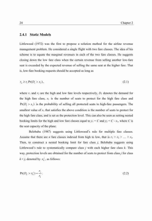
2.4.1 Static Models
Littlewood (1972) was the first to propose a solution method for the airline revenue
management problem. He considered a single flight with two fare classes. The idea of his
scheme is to equate the marginal revenues in each of the two fare classes. He suggests
closing down the low fare class when the certain revenue from selling another low-fare
seat is exceeded by the expected revenue of selling the same seat at the higher fare. That
is, low-fare booking requests should be accepted as long as
)Pr( 1112 xDrr >≥ , (2.1)
where r1 and r2 are the high and low fare levels respectively, D1 denotes the demand for
the high fare class, x1 is the number of seats to protect for the high fare class and
)Pr( 11 xD > is the probability of selling all protected seats to high-fare passengers. The
smallest value of x1 that satisfies the above condition is the number of seats to protect for
the high fare class, and is set as the protection level. This can also be seen as setting nested
booking limits for the high and low fare classes equal to y1 = C and y2 = C - x1, where C is
the seat capacity of the plane.
Belobaba (1987) suggests using Littlewood’s rule for multiple fare classes.
Assume that there are n fare classes indexed from high to low, that is r1 > r2 > … > rn.
Then, to construct a nested booking limit for fare class j, Belobaba suggests using
Littlewood’s rule to systematically compare class j with each higher fare class k. This
way, protection levels are obtained for the number of seats to protect from class j for class
k < j, denoted by jkx , as follows:
k
jjkk r
rxD => )Pr( . (2.2)

35
The Airline Revenue Management Problem and its OR Solution Techniques 25
A nested booking limit for class j is then given by: ∑−
=
−=1
1
j
k
jkj xCy , which is the total
capacity minus the seats protected from class j for the more profitable fare classes.
Belobaba introduces the term expected marginal seat revenue (EMSR) for the approach.
The method is known as the EMSR-a method. An alternative method often used in
practice is the EMSR-b method. This method aggregates the demand of the higher fare
classes rather than the individual protection levels. For this method, the combined
protection level for the classes 1 to j-1 is given by:
111 )Pr(
−−− =>
j
jjj r
rxD , (2.3)
where 1−jD is the aggregated demand for the first j-1 classes and 1−jr is the weighted
average of the fares of the first j-1 classes. A nested booking limit for class j is obtained
by: yj = C – xj-1. Although the EMSR-a and EMSR-b methods are popular and easy to use
in practice, they do not provide the theoretical optimal solution for the multiple fare class
problem. In order to obtain the number of seats to protect from class j, the EMSR-a
method aggregates the individual protection levels obtained for the fare classes higher
than j. This is not optimal because of the statistical averaging effect that occurs when
aggregating random variables. The EMSR-b method aggregates the demand before
constructing a joint protection level for all classes higher than j, but approximates the
revenue obtained by the higher fare classes somewhat roughly by its weighted average.
Under the assumption that booking requests occur in order of increasing fare, static
models that provide the theoretical optimal solution method do exist. Such optimal
policies have been presented independently by Brumelle and McGill (1993), Curry (1990)
and Wollmer (1992). Curry uses continuous demand distributions and Wollmer uses
discrete demand distributions. The approach Brumelle and McGill propose, is based on
sub-differential optimization and admits either discrete or continuous demand

36
Chapter 2 26
distributions. They show that an optimal set of nested protection levels must satisfy the
conditions:
)()( 1 jjjjj xERrxER −++ ≤≤ δδ , ∀ j = 1, 2, ..., n-1, (2.4)
where ERj(xj) is the expected revenue from the j highest fare classes when xj seats are
protected for those classes and δ+ and δ- are the right and left derivatives with respect to xj
respectively. These conditions express that a change in xj away from the optimal level in
either direction will produce a smaller increase in the expected revenue than an immediate
increase of rj+1. The same conditions apply for discrete and continuous demand
distributions. Notice, that it is only necessary to set n-1 protection levels when there are n
fare classes on the flight, because no seats will have to be protected for the lowest fare
class. Brumelle and McGill show that under certain continuity conditions the conditions
for the optimal nested protection levels reduce to the following set of probability
statements:
)Pr( 1112 xDrr >= (2.5)
)Pr( 2211113 xDDxDrr >+∩>=
)......Pr( 1121221111 −− >+++∩∩>+∩>= nnn xDDDxDDxDrr .
These statements have a simple and intuitive interpretation, much like Littlewood’s rule,
and are based on the idea of equating the marginal revenues in the various fare classes.
Robinson (1995) finds the optimality conditions when the assumption of a sequential
arrival order with monotonically increasing fares is relaxed into a sequential arrival order
with an arbitrary fare order. Furthermore, Curry (1990) provides an approach to apply his
method to a network setting. He suggests nesting the various fare classes on each route of
connecting flights and applying the single flight model to each individual route.
37
The Airline Revenue Management Problem and its OR Solution Techniques 27
Van Ryzin and McGill (2000) introduce a simple adaptive approach for finding
protection levels for multiple nested fare classes, which has the distinctive advantage that
it does not need any demand forecasting. Instead, the method uses historical observations
to guide adjustments to the protection levels. They suggest adjusting the protection level xj
upwards after each flight if all the fare classes up to j reached their protection levels, and
downwards if this has not occurred. They prove that under reasonable regularity
conditions, the algorithm converges to the optimal nested protection levels. This scheme
of continuously adjusting the protection levels has the advantage that it does not need any
demand forecasting and therefore is a way to get around all the difficulties involving this
practice. However the updating scheme does need a sufficiently large sequence of flights
to converge to a good set of protection levels. In practice, such a start-up period will
generally not be granted when there are profits to be made.
The solution methods in this paragraph are all static. This class of solution
methods can be optimal under the sequential arrival assumption as long as no change in
the probability distributions of the demand is foreseen. However, information on the
actual demand process can reduce the uncertainty associated with the estimates of
demand. Hence, repetitive use of a static method over the booking period based on the
most recent demand and capacity information is the general way to proceed.
2.4.2 Dynamic Models
Contrary to static models, dynamic models do not specify a fixed policy for use over a
longer period of time. Instead, they monitor the state of the booking process over time and
decide on acceptance of a particular booking request when it arrives, based on the state of
the booking process at that point in time.
Lee and Hersh (1993) study the standard version of the problem. They consider a
discrete-time dynamic programming model, where demand for each fare class is modelled
by a non-homogeneous Poisson process. Using a non-homogeneous Poisson process gives
rise to the use of a Markov decision model in such a way that, at any given time t, the
38
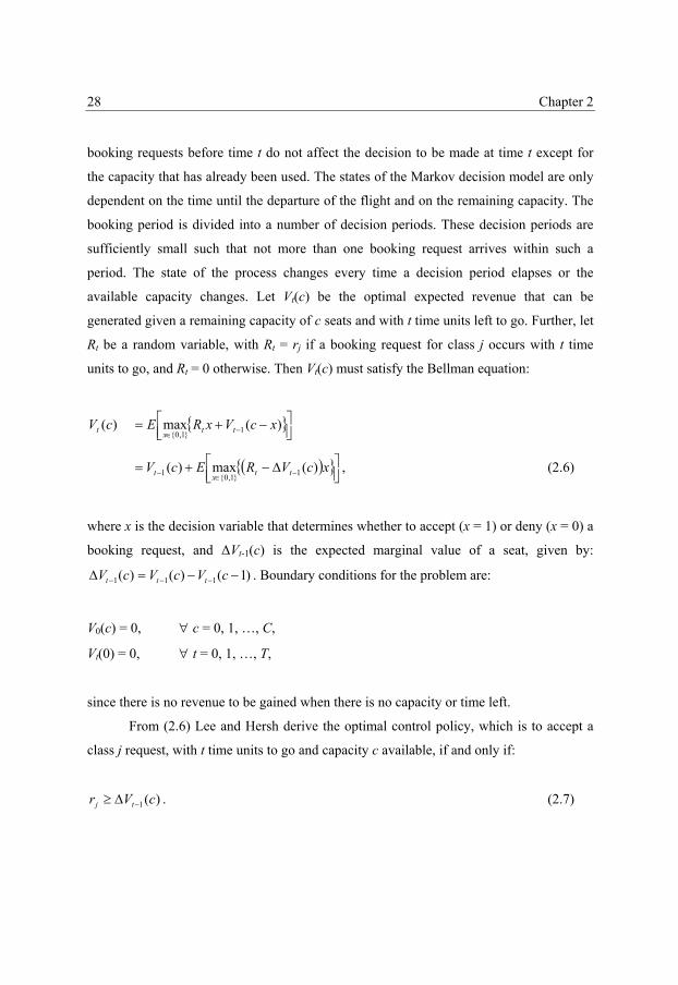
Chapter 2 28
booking requests before time t do not affect the decision to be made at time t except for
the capacity that has already been used. The states of the Markov decision model are only
dependent on the time until the departure of the flight and on the remaining capacity. The
booking period is divided into a number of decision periods. These decision periods are
sufficiently small such that not more than one booking request arrives within such a
period. The state of the process changes every time a decision period elapses or the
available capacity changes. Let Vt(c) be the optimal expected revenue that can be
generated given a remaining capacity of c seats and with t time units left to go. Further, let
Rt be a random variable, with Rt = rj if a booking request for class j occurs with t time
units to go, and Rt = 0 otherwise. Then Vt(c) must satisfy the Bellman equation:
)(cVt ⎥⎦⎤
⎢⎣⎡ −+= −∈
)(max 11,0xcVxRE ttx
( ) ⎥⎦⎤
⎢⎣⎡ ∆−+= −∈− xcVREcV ttxt )(max)( 11,01 , (2.6)
where x is the decision variable that determines whether to accept (x = 1) or deny (x = 0) a
booking request, and ∆Vt-1(c) is the expected marginal value of a seat, given by:
)1()()( 111 −−=∆ −−− cVcVcV ttt . Boundary conditions for the problem are:
V0(c) = 0, ∀ c = 0, 1, …, C,
Vt(0) = 0, ∀ t = 0, 1, …, T,
since there is no revenue to be gained when there is no capacity or time left.
From (2.6) Lee and Hersh derive the optimal control policy, which is to accept a
class j request, with t time units to go and capacity c available, if and only if:
)(1 cVr tj −∆≥ . (2.7)

39
The Airline Revenue Management Problem and its OR Solution Techniques 29
This decision rule says that a booking request is only accepted if its fare exceeds the
opportunity costs of the seat, defined here by the expected marginal value of the seat. Lee
and Hersh show that solving the model under the decision rule given by (2.7) results into a
booking policy that can be expressed as a set of critical values for either the remaining
capacity or the time until departure. For each fare class the critical values provide either an
optimal capacity level for which booking requests are no longer accepted in a given
decision period, or an optimal decision period after which booking requests are no longer
accepted for a given capacity level. The critical values are monotone over the fare classes.
Lee and Hersh also provide an extension to their model to incorporate group arrivals.
Kleywegt and Papastavrou (1998) demonstrate that the problem can also be
formulated as a dynamic and stochastic knapsack problem (DSKP). Their work is aimed at
a broader class of problems than only the single flight revenue management problem
considered here, and includes the possibility of stopping the process before time 0 with a
given terminal value for the remaining capacity, waiting costs for capacity unused and a
penalty for rejecting an item. Their model is a continuous-time model, but they only
consider homogeneous arrival processes for the booking requests. In a recent paper
Kleywegt and Papastavrou (2001) extend their model to allow for group arrivals.
Subramanian et al. (1999) extend the model proposed by Lee and Hersh to
incorporate cancellations, no-shows and overbooking. They also consider a continuous-
time arrival process as a limit to the discrete-time model by increasing the number of
decision periods. Liang (1999) reformulates and solves the Lee and Hersh model in
continuous-time. Van Slyke and Young (2000) also obtain continuous-time versions of
Lee and Hersh’ results. They do this by simplifying the DSKP model to the more standard
single flight revenue management problem and extending it for non-homogeneous arrival
processes. They also allow for group arrivals. Brumelle and Walczak (2003) extend the
problem with non-homogeneous semi-Markov arrivals which allows for correlated
demand between the fare classes. They also include group arrivals and overbooking.
Lautenbacher and Stidham (1999) link the dynamic and static approaches. They
demonstrate that a common Markov decision process underlies both approaches and
40
Chapter 2 30
formulate an omnibus model which encompasses the static and dynamic models as special
cases.
2.5 Network Models
Airlines typically offer many different flights that can be combined by a passenger in
order to reach his/her final destination. This means that an airline offers different
route/fare-class combinations, also known as origin-destination/fare-class (ODF)
combinations. As discussed in Section 2.2.1, this creates the problem of comparing
requests for routes that make use of different flights. One way to do this is to distribute the
revenue of a route over its individual flights, which is called prorating, and apply single
flight models to the individual flights. Williamson (1992) investigates different prorating
strategies, such as prorating based on mileage and on the ratio of the local fare levels. She
concludes, however, that mathematical programming models that take into account the
network of flights as a whole can produce a considerable revenue gain over simple
prorating techniques.
In Section 2.5.1 we first discuss the structure of the theoretically optimal control
policy before we present the most common mathematical programming models for
network revenue management in Section 2.5.2. In sections 2.5.3 and 2.5.4 we discuss how
nested booking-limit and bid-price policies can be constructed from the mathematical
programming models. We finish this section in Section 2.5.5 with some dynamic
approximation schemes for the network revenue management problem.
2.5.1 Optimal Control
Just as for the single flight problem, a dynamic formulation with its optimal control policy
can be formulated for the network revenue management problem. In order to do so,
consider a flight network consisting of m flights and n route/fare-class combinations. Let r

41
The Airline Revenue Management Problem and its OR Solution Techniques 31
= (r1, r2, …, rn)T, D = (D1, D2, …, Dn)T and c = (c1, c2, …, cm)T be the fares, demand and
capacities of the various route/fare-class combinations and flights. Further, define the
matrix A = [aij], such that aij = 1 whenever route/fare-class combination j uses flight i and
aij = 0 otherwise. We denote the jth column of A by Aj, which gives the capacities used by
route/fare-class combination j. Since there are generally multiple fare classes for each
route and these are all considered to be different ‘products’, multiple route/fare-class
combinations will have the same incidence vector Aj. In order to obtain the Bellman
equation for the optimal expected revenue function Vt(c), define Rt = (Rt,1, Rt,2, …, Rt,n)T as
a random vector for which Rt,j = rj if a request for class j occurs at time t, and Rt,j = 0
otherwise. Finally, let x = (x1, x2, …, xn)T be the control variable denoting whether to
accept a class j request (xj = 1) or not (xj = 0). Then, x is restricted to the set
cAxxc ≤∈= :1,0)( ntX and the Bellman equation is given by:
⎥⎦⎤
⎢⎣⎡ −+= −∈
)(max)( 1T
)(AxcxRc
cx ttXt VEVt
, (2.8)
with the boundary condition:
V0(c) = 0, ∀ c.
The optimal control policy can easily be obtained from (2.8) and says to accept a class j
booking request, with t time units to go and capacity c available, if and only if sufficient
capacity is available and:
)()( 11 jttj VVr Acc −−≥ −− . (2.9)
The optimal control policy provided here is a natural extension of the one
presented in Section 2.4.2 for the single flight case. Computationally, however, there is a
major difference between the two. Whereas the single flight optimal control policy can be

42
Chapter 2 32
calculated by backward induction for reasonable problem instances, this is
computationally far from feasible for the network case. Because of the size and the
combinatorial aspects of the network revenue management problem, obtaining a value for
one specific Vt(c) is already hard. In the next section we provide mathematical
programming models that can be used to approximate the optimal expected revenue for a
given situation.
2.5.2 Mathematical Programming Models
The mathematical programming models that we provide in this section are aimed at
finding the seat allocation that maximizes the total expected revenue of the network and
satisfies the capacity constraints on the various flights. The models can therefore be used
to approximate the value Vt(c) for a given t and c. This approximation can be used directly
for the accept/deny decision. However, the models generally also provide the means to
construct booking-limit and bid-price policies, which provide much more practical
booking control policies. The main difference between the models that we present in this
section is in the way they account for the stochastic nature of demand.
The first full network formulation of the network revenue management problem
has been proposed by Glover et al. (1982). They formulate the problem as a minimum cost
network flow problem with one set of arcs corresponding to the flights and another set
corresponding to the route/fare-class combinations. The method is aimed at finding the
flow on each arc in the network that maximizes revenue, without violating the capacity
constraints on the flights and upper-bounds posed by the demand forecasts for the
route/fare-class combinations. A drawback of the network flow formulation is that it
cannot always discriminate between the routes chosen from an origin to a destination.
Therefore, this formulation only holds when passengers are path-indifferent. The
advantage of the formulation is that it is easy to solve and can be re-optimized very fast.
A formulation of the problem that is able to distinguish between the different
routes from an origin to a destination, is given by the integer programming model

43
The Airline Revenue Management Problem and its OR Solution Techniques 33
underlying the network flow formulation. It is common practice to solve the LP relaxation
of this model rather than the integer programming problem, since the integer programming
problem is usually hard to solve when the number of decision variables and constraints is
large and the LP relaxation provides a good approximation for it. The LP relaxation of the
model is known as the deterministic linear programming (DLP) model and approximates
the optimal expected revenue as follows:
=)(cDLPtV max xr T (2.10)
s.t. cAx ≤
][0 Dx E≤≤ ,
where E[D] denotes the expected demand for the various route/fare-class combinations
and x gives the partitioning of the seat inventory. In this model, the demand is treated as if
it takes on a known value, e.g. as if it is deterministic, and no information on the demand
distributions is taken into account. Accordingly, the model produces the optimal seat
allocation if the expected demand corresponds perfectly with the actual demand. The
allocation of the seats obtained by the DLP model can be used as booking limits for an on-
line policy. Chen et al. (1998) show that )(cDLPtV provides an upper-bound for the optimal
expected revenue Vt(c). In sections 2.5.3 and 2.5.4 we discuss how to obtain nested
booking limits and bid prices based on the mathematical programming models presented
in this section.
The DLP model is a deterministic model and will never reserve more seats for a
higher fare class than the airline expects to sell on average. In fact, it does not recognize
the fact that )1Pr()Pr( +≥≥≥ kDkD jj at all. In order to determine whether reserving
more seats for more profitable route/fare-class combinations can be rewarding, it is
necessary to incorporate the stochastic nature of demand in the model. Wollmer (1986)
develops a model which incorporates probabilistic demand into a network setting. It
makes use of the same expected marginal revenue principles as Littlewood and Belobaba

44
Chapter 2 34
do for the single flight case. Therefore the model is called the EMR model. It is
formulated as follows:
=)(cEMRtV max ∑∑
==
≥jM
kj
kj
n
jj kDzr
11)Pr( (2.11)
s.t. ∑=
=jM
k
kjj zx
1 ∀ j = 1, 2, …, n
cAx ≤
10 ≤≤ kjz ∀ j = 1, 2, …, n, k = 1, 2, …, Mj,
where Mj is an upper-bound to the number of seats allocated to route/fare-class
combination j. A possible value for Mj is for example the smallest capacity remaining on
any of the flights j uses. The decision variable kjz takes on the value 1 when k seats or
more are allocated to the route/fare-class combination j and 0 otherwise. The coefficient of kjz in the objective function represents the expected marginal revenue of allocating an
additional kth seat to the route/fare-class combination. A drawback of the EMR model is
clearly the large amount of decision variables, which makes the model impractical to use.
Also, the EMR model makes use of the full distribution function of the demand for each
route/fare-class combination. Obtaining such a full distribution is often difficult and the
accuracy with which this can be done is often dubious. Chen et al. (1998) show that
)(cEMRtV provides a lower-bound for the optimal expected revenue Vt(c).
De Boer et al. (2002) introduce a variant to the EMR model for which they use a
coarser demand discretization. They link the model to stochastic programming techniques
and it is therefore known as the stochastic linear programming (SLP) model. It
incorporates the stochastic nature of demand by discretizing it to a limited number of
values: jNjjj ddd <<< ...21 , where Nj is the number of discretization points for route/fare-
class combination j. The SLP model is given by:

45
The Airline Revenue Management Problem and its OR Solution Techniques 35
=)(cSLPtV max ∑∑
==
≥jN
k
kjj
kj
n
jj dDzr
11)Pr( (2.12)
s.t. ∑=
=jN
k
kjj zx
1 ∀ j = 1, 2, …, n
cAx ≤ 110 jj dz ≤≤ ∀ j = 1, 2, …, n
10 −−≤≤ kj
kj
kj ddz ∀ j = 1, 2, …, n, k = 2, 3, …, Nj.
The decision variables kjz each accommodate for the part of the demand Dj that falls in the
interval ],( 1 kj
kj dd − . Summing the decision variables k
jz over all k, gives the total number
of seats allocated to route/fare-class combination j. The EMR model is a special case of
the SLP model that can be obtained by letting 1jd = 1 and 1−− k
jkj dd = 1 for all k = 2, 3, ...,
Mj. The SLP formulation is, however, more flexible because it allows a reduction of the
number of decision variables by choosing a limited amount of demand scenarios. If only
the expected demand is considered as a possible scenario, the SLP model reduces to the
DLP model. In fact, the DLP and EMR models can be seen as the two extremes that can
be obtained from the SLP model. The first is obtained by considering only one demand
scenario, the latter by considering all possible scenarios. The fact that )(cDLPtV provides
an upper-bound and )(cEMRtV provides a lower-bound for the optimal expected revenue
Vt(c), supports the use of the SLP model which encompasses both models. De Boer et al.
(2002) show that the SLP model produces better results than the DLP model and that
including more than 3 or 4 demand scenarios in the SLP model does not increase the
performance significantly.
The mathematical programming models discussed in this section are capable of
capturing the combinatorial aspects of the network revenue management problem. We
discuss how to derive nested booking limits and bid prices from the models in the next
sections.
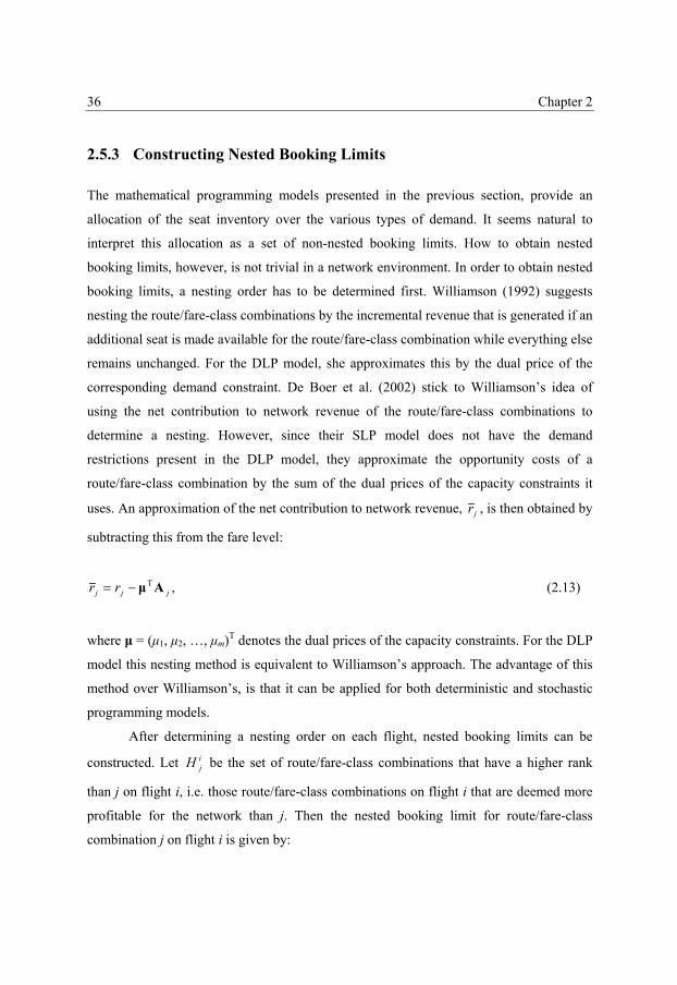
46
Chapter 2 36
2.5.3 Constructing Nested Booking Limits
The mathematical programming models presented in the previous section, provide an
allocation of the seat inventory over the various types of demand. It seems natural to
interpret this allocation as a set of non-nested booking limits. How to obtain nested
booking limits, however, is not trivial in a network environment. In order to obtain nested
booking limits, a nesting order has to be determined first. Williamson (1992) suggests
nesting the route/fare-class combinations by the incremental revenue that is generated if an
additional seat is made available for the route/fare-class combination while everything else
remains unchanged. For the DLP model, she approximates this by the dual price of the
corresponding demand constraint. De Boer et al. (2002) stick to Williamson’s idea of
using the net contribution to network revenue of the route/fare-class combinations to
determine a nesting. However, since their SLP model does not have the demand
restrictions present in the DLP model, they approximate the opportunity costs of a
route/fare-class combination by the sum of the dual prices of the capacity constraints it
uses. An approximation of the net contribution to network revenue, jr , is then obtained by
subtracting this from the fare level:
jjj rr AµT−= , (2.13)
where µ = (µ1, µ2, …, µm)T denotes the dual prices of the capacity constraints. For the DLP
model this nesting method is equivalent to Williamson’s approach. The advantage of this
method over Williamson’s, is that it can be applied for both deterministic and stochastic
programming models.
After determining a nesting order on each flight, nested booking limits can be
constructed. Let ijH be the set of route/fare-class combinations that have a higher rank
than j on flight i, i.e. those route/fare-class combinations on flight i that are deemed more
profitable for the network than j. Then the nested booking limit for route/fare-class
combination j on flight i is given by:
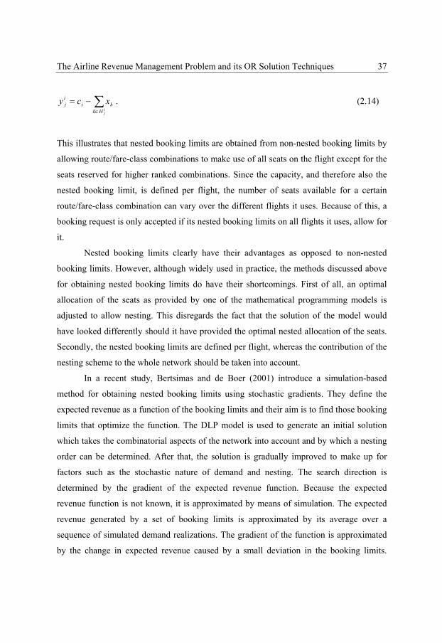
47
The Airline Revenue Management Problem and its OR Solution Techniques 37
∑∈
−=ijHk
kiij xcy . (2.14)
This illustrates that nested booking limits are obtained from non-nested booking limits by
allowing route/fare-class combinations to make use of all seats on the flight except for the
seats reserved for higher ranked combinations. Since the capacity, and therefore also the
nested booking limit, is defined per flight, the number of seats available for a certain
route/fare-class combination can vary over the different flights it uses. Because of this, a
booking request is only accepted if its nested booking limits on all flights it uses, allow for
it.
Nested booking limits clearly have their advantages as opposed to non-nested
booking limits. However, although widely used in practice, the methods discussed above
for obtaining nested booking limits do have their shortcomings. First of all, an optimal
allocation of the seats as provided by one of the mathematical programming models is
adjusted to allow nesting. This disregards the fact that the solution of the model would
have looked differently should it have provided the optimal nested allocation of the seats.
Secondly, the nested booking limits are defined per flight, whereas the contribution of the
nesting scheme to the whole network should be taken into account.
In a recent study, Bertsimas and de Boer (2001) introduce a simulation-based
method for obtaining nested booking limits using stochastic gradients. They define the
expected revenue as a function of the booking limits and their aim is to find those booking
limits that optimize the function. The DLP model is used to generate an initial solution
which takes the combinatorial aspects of the network into account and by which a nesting
order can be determined. After that, the solution is gradually improved to make up for
factors such as the stochastic nature of demand and nesting. The search direction is
determined by the gradient of the expected revenue function. Because the expected
revenue function is not known, it is approximated by means of simulation. The expected
revenue generated by a set of booking limits is approximated by its average over a
sequence of simulated demand realizations. The gradient of the function is approximated
by the change in expected revenue caused by a small deviation in the booking limits.
48
Chapter 2 38
Using simulation to find the right booking limits has the advantage that just about any
demand pattern can be accounted for. The difficulty with this method is, however, to
estimate the expected revenue function adequately. Bertsimas and de Boer also provide a
way to construct bid prices in this manner.
Whereas Bertsimas and de Boer (2001) use a discrete model of capacity and
demand, van Ryzin and Vulcano (2004) use a continuous model. This creates the
possibility to go around all the problems concerning the discrete model. For the
continuous model, van Ryzin and Vulcano are able to compute the gradient of the
expected revenue function exactly instead of using first-difference estimates. In addition,
they are able to prove that stochastic gradient methods are at least locally convergent.
2.5.4 Constructing Bid Prices
For a bid-price control policy, a bid price is set for each flight in the network reflecting the
opportunity costs of a seat. A booking request is accepted only if its fare exceeds the sum
of the bid prices of the flights it uses. Therefore, a booking request for route/fare-class
combination j, is accepted if and only if there is sufficient capacity and:
jjr AµT≥ , (2.15)
where µ = (µ1, µ2, …, µm)T are the bid prices set for the m flights. Looking at the optimal
control policy provided by (2.9), it is easy to see that a bid-price policy provides the
optimal control structure if: jjtt VV AµAcc T11 )()( =−− −− . This is the case when the
opportunity costs of the capacity taken up by the booking request are equal to the sum of
the opportunity costs of the individual flights.
The general way to approximate the opportunity costs of a seat is by the dual price
of the capacity constraint of the flight in one of the mathematical programming models
presented in Section 2.5.2. Notice that this measure is equivalent to the approximation de
49
The Airline Revenue Management Problem and its OR Solution Techniques 39
Boer et al. (2002) use for the opportunity costs of a route/fare-class combination.
Williamson (1992) uses the dual prices of the DLP model as bid prices, whereas de Boer
et al. (2002) use the bid prices of their SLP model.
Talluri and van Ryzin (1999) introduce a simulation-based method to construct bid
prices. The idea is to incorporate more stochastic information into the DLP model by
replacing the expected demand by the random vector itself. They simulate a sequence of
demand realizations and for each realization determine the optimal seat allocation. This
can be done by applying the DLP model with the realization of the demand taking the
place of the expected demand as the upper-bound for the number of bookings to accept.
This way, each simulated demand sequence provides an optimal allocation of the seats
with the corresponding dual prices. The bid price for a flight is then simply defined as the
average value of the dual prices of the flight. This is known as the randomized linear
programming (RLP) method. This method has the appealing advantage that it accounts for
the stochastic nature of demand by ways of simulation. Simulation offers the flexibility to
model various properties of the demand that would otherwise be very hard or even
impossible to model.
A disadvantage of a bid-price control policy is that the bid prices have to be
adjusted continuously. If a bid price is not adjusted regularly, this means that there is no
limit to the number of bookings that can be accepted for a route/fare-class combination
once it is open for bookings, i.e. once its fare exceeds the opportunity costs. This can lead
to flights filling up with passengers that only marginally contribute to the network
revenue. Talluri and van Ryzin (1998) provide a theoretical framework for the use of bid
prices. They show that although bid prices are not optimal in general, they are
asymptotically optimal when capacity and demand increase proportionally.
2.5.5 Dynamic Approximate Schemes
The booking control policies discussed thus far for the network revenue management
problem are all static methods. They construct a booking-limit or bid-price policy for the

50
Chapter 2 40
entire booking horizon. Although the values are generally re-adjusted a number of times
during the booking process, a model that would actually consider the fact that the policy is
adjusted over time would probably provide different values in the first place. A dynamic
programming approach to the network revenue management problem is computationally
far from feasible. However, some dynamic approximation schemes have been suggested.
Chen et al. (1998) are the first to provide a dynamic approximation scheme for the
network problem. They deduct the optimal control policy given by (2.9) and suggest to
approximate the values Vt-1(c) and Vt-1(c − Aj) directly whenever a booking request for
route/fare-class combination j is made. To approximate the values, the objective value of a
mathematical programming model can be used for both situations. Subtracting the
objective values gives the opportunity costs to which the fare can be compared. Chen et al.
(1998) argue that the opportunity costs are overestimated by the DLP model and
underestimated by the EMR model. Based on this idea, they formulate the following
acceptance scheme for a booking request for route/fare-class combination j:
reject if: EMRjr µ≤ , otherwise
accept if: DLPjr µ≥ , otherwise
accept if: rj > x, with x random from the interval [µEMR, µDLP],
where µEMR and µDLP are the opportunity costs of the request as approximated by the EMR
and DLP models. Evaluating the two models in two different states every time a booking
request comes in obviously requires too much computation time for an on-line policy.
Therefore, Chen et al. propose a method to estimate the value function of a model for each
possible state beforehand. They evaluate the model on a carefully selected limited number
of points in the state space and use these observations to estimate the value function of the
model over the entire state space. The selection of the points is based on an Orthogonal
Array method, and Multivariate Adaptive Regression Splines are used to estimate the
value function of the model. With an approximation of the value function of each model

51
The Airline Revenue Management Problem and its OR Solution Techniques 41
available at any time, decisions can be made on-line. The difficulty of this scheme is to
obtain good estimations of the value functions of the mathematical programming models.
For their simulation-based method, discussed in Section 2.5.3, Bertsimas and de
Boer (2001) also make use of an expected future revenue function. They divide the
booking period into smaller time intervals. This way, the computationally cumbersome
simulation-based method for constructing booking limits can be applied to the current
time interval only, taking into account the expected future revenue as a function of the
remaining capacity. In order to estimate the expected future revenue function, the values
for this function are evaluated over a carefully selected limited number of points in the
state space and interpolated to the entire state space.
Just as Chen et al. (1998), Bertsimas and Popescu (2003) propose to approximate
the values Vt-1(c) and Vt-1(c − Aj) directly in order to obtain an estimation of the
opportunity costs of a request. They use the network flow formulation of the problem,
proposed by Glover et al. (1982), to do this. This model is easy to solve and can be re-
optimized very efficiently. A drawback of the network flow formulation is that it only
holds when passengers are path-indifferent. Bertsimas and Popescu extend their method
with a roll-out policy using simulation techniques. For this, multiple future demand
realizations are simulated for which the revenues obtained by the current policy can be
easily computed. Averaging the revenues over the simulated demand realizations provides
an approximation of the expected future revenue that is used to approximate the current
opportunity costs. This method evades any of the problems encountered for booking
control policies discussed in the previous sections. However, although very interesting and
insightful in its own right, the computation time involved in the method is such that it
generally prevents it from being useful in practice.
2.6 Summary and Conclusion
In this chapter, we present the airline revenue management problem as it is generally
considered. We discuss the difficulties concerning uncertain demand, on-line decision

52
Chapter 2 42
making and dealing with a network of flights. We also discuss topics closely related to the
revenue management problem such as demand forecasting, overbooking and pricing.
Further, we provide an overview of OR techniques for airline revenue management under
the most common assumptions about demand behaviour. We distinguish two popular and
widely used booking control policies: booking limits and bid prices. Both policies have
their advantages and their disadvantages. Most notably, booking limits provide a robust
solution for a longer period of time, but encounter problems with nesting. Bid prices on
the other hand are closely related to the theoretically optimal control policy but need to be
adjusted frequently. Neither of the policies is optimal, but they can be proven to be
asymptotically optimal and are easy to use in practice.
The mathematical models used for single flight and network revenue management
problems, are somewhat different. For the single flight case, simple static models based on
the expected marginal value of a seat can be easily constructed for use in practice.
Dynamic models can also be constructed and their optimal policy can be proven to possess
nice structural properties as long as group arrivals and overbooking are not allowed. For
practical use, however, the dynamic models are generally less feasible.
Because of the combinatorial aspects involved with the network revenue
management problem, mathematical programming models are generally used for this
problem. We present three of such models that vary in the manner that the uncertainty of
the demand is accounted for. Based on the mathematical programming models, nested
booking limits and bid prices can be constructed. We discuss various ways to do so that all
have their stronger and weaker aspects. Dynamic models are computationally not feasible
for the network problem. We do discuss some dynamic approximation schemes. However,
the question remains whether the problems they encounter in order to get around the
computational difficulties do not outweigh the positive effect of capturing the dynamics of
the booking process.
Despite the level of attention for the airline revenue management problem
throughout the years, some issues are still open for improvement. Recent studies have
concentrated on finding better ways to construct booking limits and bid prices in a
network environment (see: Bertsimas and de Boer (2001) and van Ryzin and Vulcano

53
The Airline Revenue Management Problem and its OR Solution Techniques 43
(2004)) or estimating the expected future revenue function for dynamic approximation
schemes for the network problem (see: Bertsimas and de Boer (2001), Bertsimas and
Popescu (2003) and Chen et al. (1998)). These problems certainly provide issues for future
research. The majority of the current research in airline revenue management, however, is
aimed at relaxing one or more of the assumptions about demand behaviour discussed in
Section 2.2.3 (see the references given in Section 2.2.3). Although conceptually very
interesting, these studies are generally restricted to the single flight and often even two
fare class case of the problem, which is far from practice.
As mentioned in the introduction, the airline revenue management problem as
discussed in this chapter forms the basis for most other well-known revenue management
applications. The models presented in Sections 2.4 and 2.5 are widely used for
applications in the hotel, railroad and car rental industries with only minor adjustments.

54

55
Chapter 3 Models and Techniques for Hotel Revenue Management using a Rolling Horizon
3.1 Introduction
After the airline industry, the hotel industry is the second most popular application area of
revenue management. As the success story of revenue management started to reach
beyond the airline industry, hotels were quick to recognize the similarities between selling
the seats on a plane to different types of passengers for different prices, and the situation
hotels face when renting rooms. In this chapter, we provide models and techniques for
hotel revenue management. We present both deterministic and stochastic mathematical
programming models of which the latter has not been applied before to the hotel revenue
management problem. We construct booking-limit and bid-price control policies based on
the deterministic and stochastic models. We also construct randomized bid prices by
simulation techniques. The performance of the booking control polices is evaluated in a
simulated environment. Unlike previous studies, we extend the booking control policies

56
Chapter 3 46
with a rolling horizon of overlapping decision periods which conveniently captures the
effects of overlapping stays.
In Section 3.2 we discuss the hotel revenue management problem and the literature
presented on it. We present the mathematical models in Section 3.3 and the booking
control policies based on them in Section 3.4. In Section 3.5 we describe the test case we
construct in order to evaluate the different booking control policies. Finally, we present
the results of our simulation study in Section 3.6 and conclude this chapter in Section 3.7.
3.2 Hotel Revenue Management
In the hotel industry different prices are charged for a room depending on features such as:
the time of booking, company affiliation, multiple-day stays and the intermediary sales
agent. This way, hotels offer the same rooms to different types of guests for different
prices. While hotel managers would like to fill their hotels with highly profitable guests as
much as possible, it is generally also necessary to allow for less profitable guests in order
to prevent rooms from remaining vacant. The number of low-price guests in the hotel
should be managed carefully, however, in order to be able to allocate as many high-price
guests as possible. The booking requests come in gradually over time and the decision
whether to accept a certain booking request or not has to be made at the moment it comes
in. This is known as the hotel revenue management problem and resembles the airline
problem discussed in the previous chapter.
In Section 3.2.1 we shortly discuss some of the difficulties in hotel revenue
management and in Section 3.2.2 we provide an overview of the related literature on the
problem.
57
Models and Techniques for Hotel Revenue Management using a Rolling Horizon 47
3.2.1 Difficulties in Hotel Revenue Management
Many of the problems concerning revenue management in the airline industry, i.e.
uncertain demand, on-line decision making and network effects, also apply to the hotel
industry. The uncertainty of demand and the on-line decision making process are
difficulties that directly translate to the hotel revenue management problem. They bring
stochastic and dynamic aspects into the problem. Also the network effects caused in the
airline industry by the network of flights that an airline typically offers, has its
correspondence in the hotel industry. These network effects are caused by the fact that
guests in a hotel can stay multiple days such that their stays can overlap. Consider for
example, one guest staying from Monday to Friday and another from Thursday to Sunday.
Then, the guests compete for the same room capacity on Thursday and Friday. Although a
hotel manager would like to fill his hotel with guests who pay a high price, it can be more
profitable to accept a lower price request when this request would also fill up capacity for
other days where demand is low. Conceptually, a guest that stays in a hotel for multiple
days can be seen as a passenger that uses multiple flights to reach his/her destination.
However, whereas the flights offered by an airline span a finite network that is observed at
a given point in time, the different stays in a hotel can continue to overlap over an infinite
horizon. This means that no fixed decision period can be determined without missing
some of the effects of the overlapping stays. Therefore, we apply the booking control
policies over a rolling horizon of overlapping decision periods where all booking types
that are open for booking are taken into account.
Another problem in hotel revenue management is that the room rates do not always
provide the total profit associated to a guest. Often, profits generated by the bar,
restaurant, casino or other facilities that a hotel offers, can be quite significant. Therefore,
it is very interesting for a hotel to recognize the true profitability of a booking request.
Tools such as a client ID card can provide a means for this. In practice, however, it is very
difficult to estimate the full profitability of a booking request beforehand. For the
remainder of this chapter we consider the profitability of a booking request to be given by
its room rate.

58
Chapter 3 48
Next to the fact that we assume the profitability of a booking request to be given
by the price it pays for the room, we make use of the common assumptions in quantity-
based revenue management that the room capacity and the general price structure are
given and fixed. We also assume that there is a limit to the number of days that a guest can
stay in the hotel and to the number of days that a booking can be made in advance. The
first does not have to be imposed by the hotel explicitly but can rather be a natural bound
observed in practice caused by the fact that guests will eventually leave the hotel. The
second is generally determined by the reservation system that has a limited planning
horizon. Further, we consider the general assumptions about demand behaviour. This
means that we do not consider group bookings, cancellations and no-shows and assume
that demand is independent of the booking control policy used. This last assumption has
been the subject of debate but is difficult to relax. We refer to Section 2.2.3 for some
references to studies that relax the assumption for the airline problem.
3.2.2 Literature
Hotel revenue management has received attention in a number of papers. Bitran and
Mondschein (1995) and Bitran and Gilbert (1996) concentrate on the room allocation
problem at the targeted booking day. This means that they concentrate on the stays that
start on the current day itself. The hotel manager has to decide whether or not to accept a
guest who shows up without a reservation (walk-in), taking into account the number of
reservations already made and the potential number of remaining walk-ins. They
formulate this problem as a stochastic and dynamic programming model. Bitran and
Gilbert also provide three simple heuristics to construct booking control policies that can
be used during the booking period.
Weatherford (1995) concentrates on a booking control policy for the booking
period. He constructs booking limits based on a deterministic mathematical programming
model similar to the one discussed in Section 2.5 for the airline problem. The booking
limits are nested based on the dual prices of the model such that a booking request can

59
Models and Techniques for Hotel Revenue Management using a Rolling Horizon 49
always make use of the capacity reserved for any booking request that is considered to be
less profitable. A drawback of this policy is that it considers demand to be deterministic.
Weatherford allows for multiple-day stays and optimizes the model for a decision period
consisting of a fixed set of target booking days. He does not account for overlapping stays
that fall outside the set of target booking days. Nevertheless, he shows that taking into
account multiple-day stays explicitly produces better results than when they are
considered as a set of single-day stays.
Baker and Collier (1999) compare the performance of five booking control
policies: two simple threshold approaches, the deterministic nested booking-limit policy
proposed by Weatherford, the deterministic nested booking-limit policy that includes
overbooking and finally a deterministic bid-price policy obtained from Weatherford’s
deterministic model. Baker and Collier compare the performance of the booking control
policies under 36 hotel operating environments by means of simulation and advise on the
best heuristic for each operating environment.
In this chapter we concentrate on the booking control problem. This makes our
work comparable to the work of Weatherford (1995) and Baker and Collier (1999). Unlike
these previous studies, we use the booking control policies over a rolling horizon of
decision periods, such that all overlap between the different types of stay can be accounted
for. Also, next to the booking control policies based on the well-known deterministic
model, we obtain bid prices that account for demand uncertainty by simulation and we
obtain nested booking limits and bid prices based on a mathematical programming model
that accounts for the stochastic nature of demand. As Baker and Collier (1999), we
compare the performance of the different methods in a simulated environment.
3.3 Mathematical Programming Models
The booking control policies that we consider for the hotel revenue management problem
are based on an optimal allocation of the demand for a fixed set of target booking days. In
this section, we present two mathematical programming models that can provide such an
60
Chapter 3 50
allocation. The models differ in the way that they take demand into account. In Section
3.3.1 we discuss a deterministic model that only considers a point estimate of the demand.
In Section 3.3.2 we present a stochastic model that considers a discretization of the
demand distribution.
3.3.1 Deterministic Model
The deterministic model that we consider is the same as Weatherford (1995) proposes for
his nested booking-limit policy. This model uses the expected demand as a point estimate
of the demand and obtains the optimal allocation of the rooms for it. This means that it
treats demand as if it were deterministic and equal to its expectation. To formulate the
model, we note that each type of booking request is defined by three aspects: its price
class, its starting day and its length of stay. We consider n of such booking types. Further,
we let the decision period of the model consist of m target booking days. Let r = (r1, r2,
…, rn)T, D = (D1, D2, …, Dn)T and c = (c1, c2, …, cm)T denote the prices, demand and
capacities of the various booking types and days. Further, we define the matrix A = [aij],
such that aij = 1 if booking type j stays on day i and aij = 0 otherwise. We denote the jth
column of A by Aj, which gives the capacities used by booking type j and consists of
exactly as many 1 entries as the number of days that the guest wishes to stay in the hotel.
The deterministic mathematical programming model can now be formulated as follows:
max xr T (3.1)
s.t. cAx ≤
][0 Dx E≤≤ ,
where E[D] denotes the expected demand for the various booking types and x gives the
partitioning of the room capacity. The objective of the model is to maximize revenues
under the restriction that the total number of reservations for a day does not exceed the
room capacity for that day. The number of rooms allocated to each booking type is

61
Models and Techniques for Hotel Revenue Management using a Rolling Horizon 51
restricted by the level of the demand, which in this model is replaced by its expectation. If
demand actually corresponds with its expectation, the deterministic model provides the
optimal room allocation.
Since it is usually difficult to optimize an integer programming model, the decision
variables are generally not restricted to be integer. Although the constraint matrix is not
totally unimodular, previous experiences of Williamson (1992) and de Boer et al. (2002)
with the LP model in (3.1) show that when demand and capacity is integer, the optimal
solution often is as well. When the model produces a fractional solution, however, it will
generally not take much effort to produce an integer solution by applying branch-and-
bound techniques.
3.3.2 Stochastic Model
The deterministic model approximates the distribution of the demand by a point estimate
of its expectation. This means that it assumes 1)Pr( =≥ dD j ∀ ][ jDEd ≤ and
0)Pr( =≥ dD j ∀ ][ jDEd > , ∀ j = 1, 2, …, n. In reality, however, the distribution
function is a smoothly decreasing function. Using such a rough estimate as the
deterministic model does, means that the probability of another type j arrival is
overestimated (by the value 1) as the number of arrivals has not reached its expectation yet
and underestimated (by the value 0) as the expected number of arrivals has been reached.
In this section we present a mathematical programming model that approximates the
distribution function of demand more smoothly. This stochastic model was first
introduced by De Boer et al. (2002) for the airline industry. The model incorporates the
stochastic nature of demand by discretizing it to a limited number of values: jN
jjj ddd <<< ...21 , where Nj is the number of discretization points for booking type j. The
stochastic model is then given by:
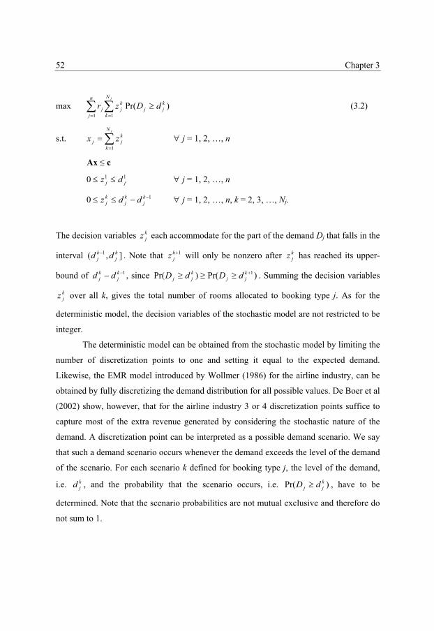
62
Chapter 3 52
max ∑∑==
≥jN
k
kjj
kj
n
jj dDzr
11)Pr( (3.2)
s.t. ∑=
=jN
k
kjj zx
1 ∀ j = 1, 2, …, n
cAx ≤ 110 jj dz ≤≤ ∀ j = 1, 2, …, n
10 −−≤≤ kj
kj
kj ddz ∀ j = 1, 2, …, n, k = 2, 3, …, Nj.
The decision variables kjz each accommodate for the part of the demand Dj that falls in the
interval ],( 1 kj
kj dd − . Note that 1+k
jz will only be nonzero after kjz has reached its upper-
bound of 1−− kj
kj dd , since )Pr()Pr( 1+≥≥≥ k
jjkjj dDdD . Summing the decision variables
kjz over all k, gives the total number of rooms allocated to booking type j. As for the
deterministic model, the decision variables of the stochastic model are not restricted to be
integer.
The deterministic model can be obtained from the stochastic model by limiting the
number of discretization points to one and setting it equal to the expected demand.
Likewise, the EMR model introduced by Wollmer (1986) for the airline industry, can be
obtained by fully discretizing the demand distribution for all possible values. De Boer et al
(2002) show, however, that for the airline industry 3 or 4 discretization points suffice to
capture most of the extra revenue generated by considering the stochastic nature of the
demand. A discretization point can be interpreted as a possible demand scenario. We say
that such a demand scenario occurs whenever the demand exceeds the level of the demand
of the scenario. For each scenario k defined for booking type j, the level of the demand,
i.e. kjd , and the probability that the scenario occurs, i.e. )Pr( k
jj dD ≥ , have to be
determined. Note that the scenario probabilities are not mutual exclusive and therefore do
not sum to 1.
63
Models and Techniques for Hotel Revenue Management using a Rolling Horizon 53
3.4 Booking Control Policies
The mathematical programming models presented in the previous section form the basis
for the booking control policies that we consider. In Section 3.4.1 we discuss how we
construct nested booking limits from the models and in Section 3.4.2 how we obtain bid
prices. In Section 3.4.3 we discuss how to use these booking control policies over a rolling
horizon of decision periods.
3.4.1 Nested Booking Limits
The number of rooms allocated to each booking type by the models from the previous
section, can easily be interpreted as booking limits. These limits can be used as the
maximum number of booking requests to accept for each booking type during the booking
period. It is never optimal, however, to reject a booking request when rooms are still
available for other less profitable booking types, even if its own booking limit has been
reached. Therefore, each booking type should be allowed to tap into the rooms allocated to
any booking type that is less profitable. When this is allowed, the booking limits are called
nested. In order to form nested booking limits, the different booking types need to be
ranked by their contribution to the overall revenue of the hotel. When such a ranking is
determined, a nested booking limit for a booking type can be determined by the sum of the
rooms allocated to it and every other, lower ranked booking type.
It is not trivial what measurement to use when determining a nesting order for the
different booking types. Using the price class does not take into account the length of the
stay. Such a measurement will rank guests who are willing to pay more for one day above
guests who are willing to pay a little less for multiple days, whereas the overall revenue
generated by the multiple days will most likely be higher. Nesting by the complete
revenue generated by the stay does take into account the length of the stay. But this
measurement does not account for the load factors of the different days. Certain days can
be very busy and always fully booked, whereas other days can be mainly vacant. A stay

64
Chapter 3 54
that occupies many busy days should be valued differently from a stay that uses mainly
days with a lot of vacant rooms. One way to take into account all of these aspects, is to use
the dual prices obtained from the underlying allocation model. The dual price
corresponding to the capacity restriction for a day reflects the expected gain that can be
obtained if one additional room were available on that day. It can be interpreted as the
opportunity costs of a room. Adding the dual prices of all the days used by a stay, gives an
indication of the opportunity costs of the stay. A measurement for nesting is then obtained
by subtracting these opportunity costs from the revenue generated by the stay. Thus, a
nesting order is based on:
jjj rr AµT−= , (3.3)
where µ = (µ1, µ2, …, µm)T denotes the dual prices of the capacity constraints. Nested
booking limits can now easily be constructed for the deterministic and stochastic models,
which we will call the Deterministic Nested Booking Limits (DNBL) and the Stochastic
Nested Booking Limits (SNBL) methods.
3.4.2 Bid Prices
The second type of booking control policy we study in this paper is the bid-price policy.
This policy directly links the opportunity costs of a stay to the acceptance/rejection
decision. A bid price is constructed for every day to reflect the opportunity costs of renting
a room on that day. As before, we estimate the opportunity costs of renting a room on a
particular day by the dual price of the capacity constraint for that day in the underlying
mathematical programming model. A booking request is only accepted if the revenue it
generates is greater than the sum of the bid prices of the days it uses. This means that a
booking request for type j, is accepted if and only if there is sufficient capacity and:
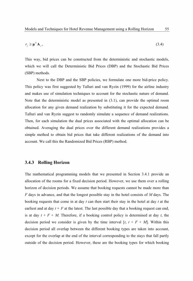
65
Models and Techniques for Hotel Revenue Management using a Rolling Horizon 55
jjr AµT≥ , (3.4)
This way, bid prices can be constructed from the deterministic and stochastic models,
which we will call the Deterministic Bid Prices (DBP) and the Stochastic Bid Prices
(SBP) methods.
Next to the DBP and the SBP policies, we formulate one more bid-price policy.
This policy was first suggested by Talluri and van Ryzin (1999) for the airline industry
and makes use of simulation techniques to account for the stochastic nature of demand.
Note that the deterministic model as presented in (3.1), can provide the optimal room
allocation for any given demand realization by substituting it for the expected demand.
Talluri and van Ryzin suggest to randomly simulate a sequence of demand realizations.
Then, for each simulation the dual prices associated with the optimal allocation can be
obtained. Averaging the dual prices over the different demand realizations provides a
simple method to obtain bid prices that take different realizations of the demand into
account. We call this the Randomized Bid Prices (RBP) method.
3.4.3 Rolling Horizon
The mathematical programming models that we presented in Section 3.4.1 provide an
allocation of the rooms for a fixed decision period. However, we use them over a rolling
horizon of decision periods. We assume that booking requests cannot be made more than
F days in advance, and that the longest possible stay in the hotel consists of M days. The
booking requests that come in at day t can then start their stay in the hotel at day t at the
earliest and at day t + F at the latest. The last possible day that a booking request can end,
is at day t + F + M. Therefore, if a booking control policy is determined at day t, the
decision period we consider is given by the time interval [t, t + F + M]. Within this
decision period all overlap between the different booking types are taken into account,
except for the overlap at the end of the interval corresponding to the stays that fall partly
outside of the decision period. However, these are the booking types for which booking
66
Chapter 3 56
has only just opened. First of all, hardly any booking requests will come in this early in the
booking process except for some extremely early bookings. Second, since booking has
just started for those target booking days, the hotel will be nearly empty for those days and
critical decisions will not have to be made yet. By the time critical decisions have to be
made for these days, the decision period will have rolled forward and have captured all
overlap between the neighbouring days.
The booking control policy is constructed at different points in time. Every time a
new policy is constructed, the decision period rolls forward. The booking limits for the
booking types that were already available for booking are adjusted, while new booking
limits are constructed for the booking types that have just opened for booking. In the same
manner, the bid prices for the days already in the decision period are adjusted, while new
bid prices are constructed for the newly added days.
3.5 Description of the Test Case
The performance of the different booking control policies is evaluated by ways of
simulation. In this section, we discuss the simulation environment. This is chosen such
that it reflects the situation described to us by a hotel in the Netherlands. We consider a
hotel with a total capacity of 150 identical rooms. These rooms can be rented out in 10
different price classes, described in Table 3.1. We consider that the maximal length of a
stay is 7 days and that a booking request can be made at most 13 weeks in advance. We do
not allow overbooking and do not consider cancellations, no-shows or group bookings.
The booking control policies that we consider are updated on a weekly basis. But we
shortly discuss the effects of doing this less or more often.
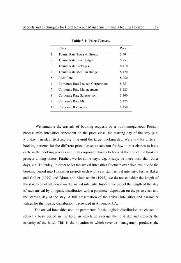
67
Models and Techniques for Hotel Revenue Management using a Rolling Horizon 57
Table 3.1: Price Classes.
Class Price
1 Tourist Rate Tours & Groups $ 50
2 Tourist Rate Low Budget $ 75
3 Tourist Rate Packages $ 110
4 Tourist Rate Medium Budget $ 120
5 Rack Rate $ 250
6 Corporate Rate Liaison Corporation $ 75
7 Corporate Rate Management $ 125
8 Corporate Rate Salesperson $ 100
9 Corporate Rate MCI $ 175
10 Corporate Rate other $ 150
We simulate the arrivals of booking requests by a non-homogeneous Poisson
process with intensities dependent on the price class, the starting day of the stay (e.g.
Monday, Tuesday, etc.) and the time until the target booking day. We allow for different
booking patterns for the different price classes to account for low tourist classes to book
early in the booking process and high corporate classes to book at the end of the booking
process among others. Further, we let some days, e.g. Friday, be more busy than other
days, e.g. Thursday. In order to let the arrival intensities fluctuate over time, we divide the
booking period into 10 smaller periods each with a constant arrival intensity. Just as Baker
and Collier (1999) and Bitran and Mondschein (1995), we do not consider the length of
the stay to be of influence on the arrival intensity. Instead, we model the length of the stay
of each arrival by a logistic distribution with a parameter dependent on the price class and
the starting day of the stay. A full presentation of the arrival intensities and parameter
values for the logistic distribution is provided in Appendix 3.A.
The arrival intensities and the parameters for the logistic distribution are chosen to
reflect a busy period in the hotel in which on average the total demand exceeds the
capacity of the hotel. This is the situation in which revenue management produces the

68
Chapter 3 58
highest gains in revenue. The average level of the demand per day of the week expressed
as a percentage of the capacity is presented in Figure 3.1. Note that one booking request
can generate demand for multiple days. Figure 3.1 shows that in our test case Friday is the
busiest day of the week with an average demand which exceeds capacity by more than
70%. On Thursday the average demand is only just above the capacity of the hotel, which
makes it the least busy day of the week.
Figure 3.1: Average demand per day of the week as percentage of the capacity.
0%
50%
100%
150%
200%
Mon Tue Wed Thur Fri Sat Son
dem
and
as p
erce
ntag
e of
cap
acity
We compare the performance of the different booking control policies over a 6
week period. Since the hotel is empty at the beginning of the simulation, the booking
control policies that are constructed at that time are not representative for the general
situation. To be representative, they would have to consider the overlap of the guests
already in the hotel based on prior booking decisions. In order to do so, we make use of a
start-up period in which the simulation can reach a steady state before the start of the 6
evaluation weeks. Since the booking control policies remain fixed for a week and the
maximum length of stay is also a week, the guests that are accepted by the initial non-
representative booking control policies can overlap until the end of the second week. In
order to refrain from all such guests in the evaluation period, we choose the start-up period
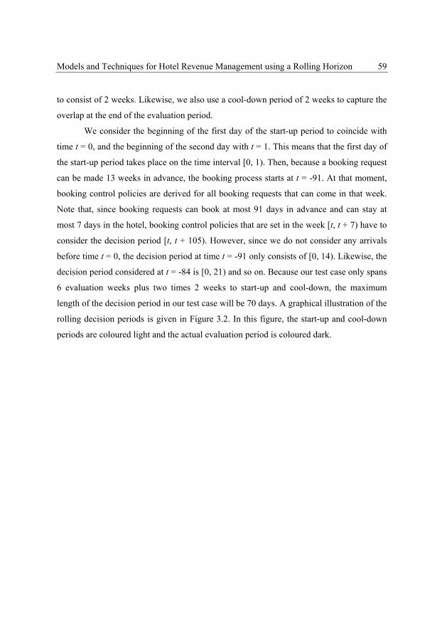
69
Models and Techniques for Hotel Revenue Management using a Rolling Horizon 59
to consist of 2 weeks. Likewise, we also use a cool-down period of 2 weeks to capture the
overlap at the end of the evaluation period.
We consider the beginning of the first day of the start-up period to coincide with
time t = 0, and the beginning of the second day with t = 1. This means that the first day of
the start-up period takes place on the time interval [0, 1). Then, because a booking request
can be made 13 weeks in advance, the booking process starts at t = -91. At that moment,
booking control policies are derived for all booking requests that can come in that week.
Note that, since booking requests can book at most 91 days in advance and can stay at
most 7 days in the hotel, booking control policies that are set in the week [t, t + 7) have to
consider the decision period [t, t + 105). However, since we do not consider any arrivals
before time t = 0, the decision period at time t = -91 only consists of [0, 14). Likewise, the
decision period considered at t = -84 is [0, 21) and so on. Because our test case only spans
6 evaluation weeks plus two times 2 weeks to start-up and cool-down, the maximum
length of the decision period in our test case will be 70 days. A graphical illustration of the
rolling decision periods is given in Figure 3.2. In this figure, the start-up and cool-down
periods are coloured light and the actual evaluation period is coloured dark.
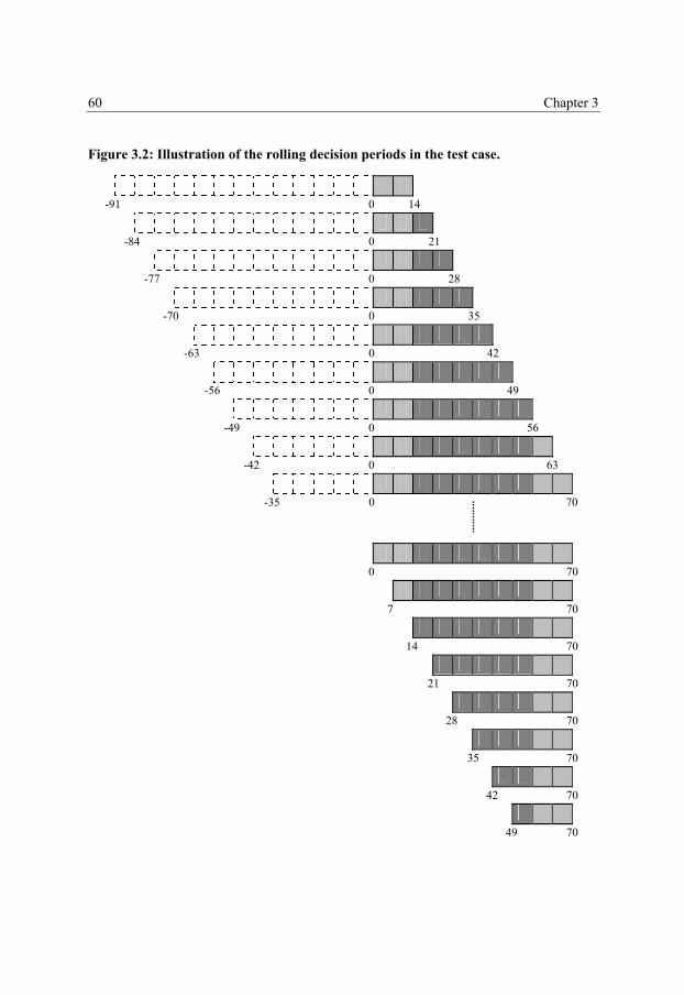
70
Chapter 3 60
Figure 3.2: Illustration of the rolling decision periods in the test case.
-91 0 14
0
0
0
0
0
0
0
0
0
21
28
35
42
49
56
63
70
70
70
70
70
70
70
70
70
-84
-77
-70
-63
-56
-49
-42
-35
7
14
21
28
35
42
49

71
Models and Techniques for Hotel Revenue Management using a Rolling Horizon 61
In conclusion, we summarize the aspects that define the simulation environment in Table
3.2.
Table 3.2: Specification of the test case.
10 price classes
150 identical rooms
max 7 day stay
max 90 days in advance booking
6 week evaluation period
2 week start-up and cool-down periods
demand exceeds capacity
different booking patterns for the different price classes
demand is independent of the booking control policies
no overbooking
no cancellations and no-shows
no group bookings
3.6 Computational Results
In Section 3.4, we specified the following five booking control policies:
• Deterministic Nested Booking Limits (DNBL)
• Deterministic Bid Prices (DBP)
• Stochastic Nested Booking Limits (SNBL)
• Stochastic Bid Prices (SBP)
• Randomized Bid Prices (RBP)
We evaluate the performance of these five booking control policies when they are applied
to the simulated environment discussed in the previous section. In Section 3.6.1 we report
the results for the DNBL, DBP and RBP methods which are all based on the deterministic

72
Chapter 3 62
mathematical programming model. In Section 3.6.2 we report results for the SNBL and
SBP methods for various demand discretizations for the stochastic mathematical
programming model. The computations discussed in the following sections are performed
on a Pentium III 550 MHz personal computer (256 MB RAM), using CPlex 7.1 to
optimize the mathematical programming models. All computation times are reported in
seconds.
3.6.1 Deterministic and Randomized Booking Control Policies
The deterministic and randomized booking control policies make use of the deterministic
model provided in (3.1) to construct a booking control policy. The DNBL and DBP
policies do so by optimizing the model once for the expected demand. The RBP policy
optimizes the model a number of times for a set of randomly generated demand
realizations and uses the average of the dual prices provided by the model. We use 100
demand realizations for this randomization technique. We measure the performance of the
booking control policies over another 100 simulated arrival processes using equal random
numbers for all policies. We compare the results with those obtained by a simple First
Come First Serve (FCFS) policy and with the optimal acceptance policy which can be
determined with hindsight. The performance of the booking control policies is presented
in Table 3.3. The averages and standard deviations presented in Table 3.3 are taken over
the 100 simulations.
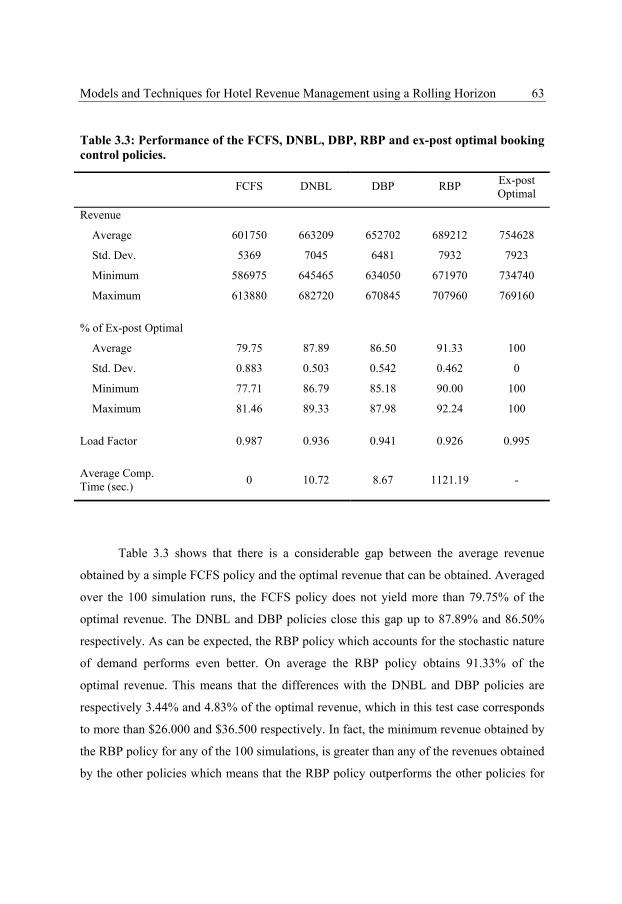
73
Models and Techniques for Hotel Revenue Management using a Rolling Horizon 63
Table 3.3: Performance of the FCFS, DNBL, DBP, RBP and ex-post optimal booking control policies.
Ex-post FCFS DNBL DBP RBP Optimal
Revenue
Average 601750 663209 652702 689212 754628
Std. Dev. 5369 7045 6481 7932 7923
Minimum 586975 645465 634050 671970 734740
Maximum 613880 682720 670845 707960 769160
% of Ex-post Optimal
Average 79.75 87.89 86.50 91.33 100
Std. Dev. 0.883 0.503 0.542 0.462 0
Minimum 77.71 86.79 85.18 90.00 100
Maximum 81.46 89.33 87.98 92.24 100
Load Factor 0.987 0.936 0.941 0.926 0.995
Average Comp. Time (sec.) 0 10.72 8.67 1121.19 -
Table 3.3 shows that there is a considerable gap between the average revenue
obtained by a simple FCFS policy and the optimal revenue that can be obtained. Averaged
over the 100 simulation runs, the FCFS policy does not yield more than 79.75% of the
optimal revenue. The DNBL and DBP policies close this gap up to 87.89% and 86.50%
respectively. As can be expected, the RBP policy which accounts for the stochastic nature
of demand performs even better. On average the RBP policy obtains 91.33% of the
optimal revenue. This means that the differences with the DNBL and DBP policies are
respectively 3.44% and 4.83% of the optimal revenue, which in this test case corresponds
to more than $26.000 and $36.500 respectively. In fact, the minimum revenue obtained by
the RBP policy for any of the 100 simulations, is greater than any of the revenues obtained
by the other policies which means that the RBP policy outperforms the other policies for
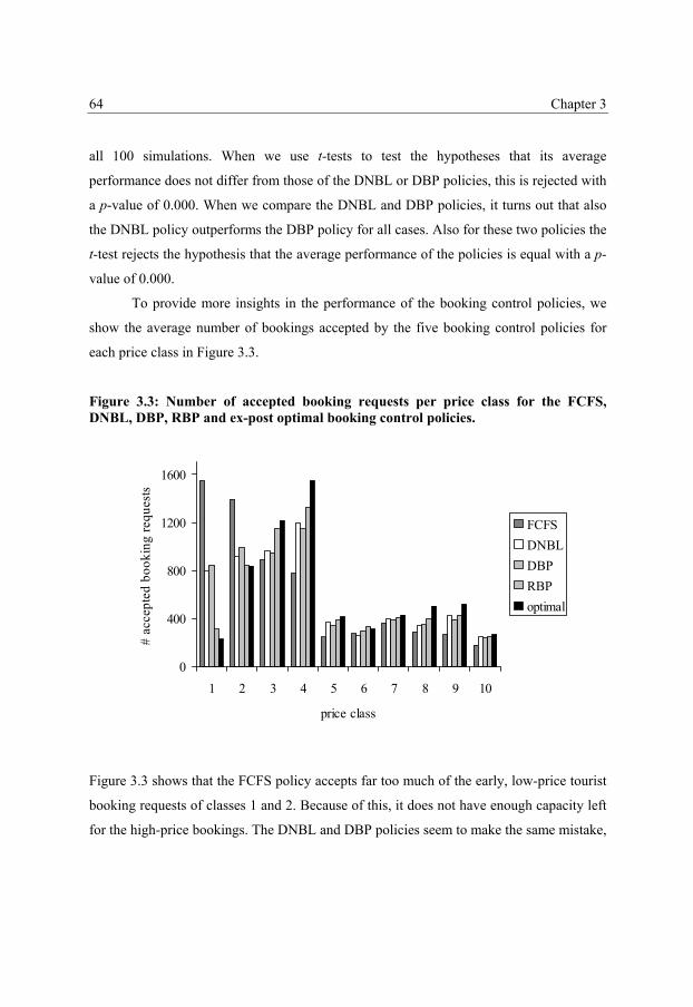
74
Chapter 3 64
all 100 simulations. When we use t-tests to test the hypotheses that its average
performance does not differ from those of the DNBL or DBP policies, this is rejected with
a p-value of 0.000. When we compare the DNBL and DBP policies, it turns out that also
the DNBL policy outperforms the DBP policy for all cases. Also for these two policies the
t-test rejects the hypothesis that the average performance of the policies is equal with a p-
value of 0.000.
To provide more insights in the performance of the booking control policies, we
show the average number of bookings accepted by the five booking control policies for
each price class in Figure 3.3.
Figure 3.3: Number of accepted booking requests per price class for the FCFS, DNBL, DBP, RBP and ex-post optimal booking control policies.
0
400
800
1200
1600
1 2 3 4 5 6 7 8 9 10
price class
# ac
cept
ed b
ooki
ng re
ques
ts
FCFSDNBLDBPRBPoptimal
Figure 3.3 shows that the FCFS policy accepts far too much of the early, low-price tourist
booking requests of classes 1 and 2. Because of this, it does not have enough capacity left
for the high-price bookings. The DNBL and DBP policies seem to make the same mistake,
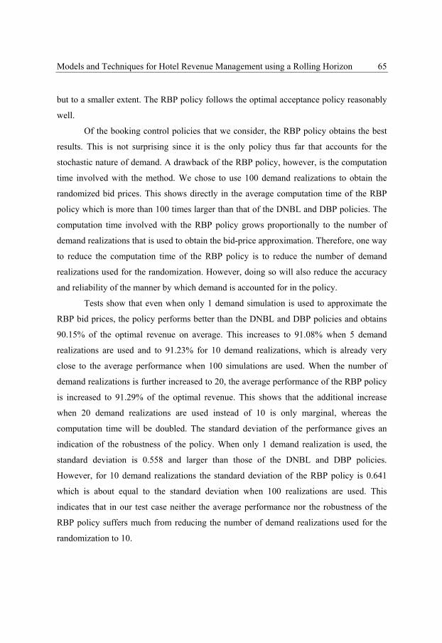
75
Models and Techniques for Hotel Revenue Management using a Rolling Horizon 65
but to a smaller extent. The RBP policy follows the optimal acceptance policy reasonably
well.
Of the booking control policies that we consider, the RBP policy obtains the best
results. This is not surprising since it is the only policy thus far that accounts for the
stochastic nature of demand. A drawback of the RBP policy, however, is the computation
time involved with the method. We chose to use 100 demand realizations to obtain the
randomized bid prices. This shows directly in the average computation time of the RBP
policy which is more than 100 times larger than that of the DNBL and DBP policies. The
computation time involved with the RBP policy grows proportionally to the number of
demand realizations that is used to obtain the bid-price approximation. Therefore, one way
to reduce the computation time of the RBP policy is to reduce the number of demand
realizations used for the randomization. However, doing so will also reduce the accuracy
and reliability of the manner by which demand is accounted for in the policy.
Tests show that even when only 1 demand simulation is used to approximate the
RBP bid prices, the policy performs better than the DNBL and DBP policies and obtains
90.15% of the optimal revenue on average. This increases to 91.08% when 5 demand
realizations are used and to 91.23% for 10 demand realizations, which is already very
close to the average performance when 100 simulations are used. When the number of
demand realizations is further increased to 20, the average performance of the RBP policy
is increased to 91.29% of the optimal revenue. This shows that the additional increase
when 20 demand realizations are used instead of 10 is only marginal, whereas the
computation time will be doubled. The standard deviation of the performance gives an
indication of the robustness of the policy. When only 1 demand realization is used, the
standard deviation is 0.558 and larger than those of the DNBL and DBP policies.
However, for 10 demand realizations the standard deviation of the RBP policy is 0.641
which is about equal to the standard deviation when 100 realizations are used. This
indicates that in our test case neither the average performance nor the robustness of the
RBP policy suffers much from reducing the number of demand realizations used for the
randomization to 10.
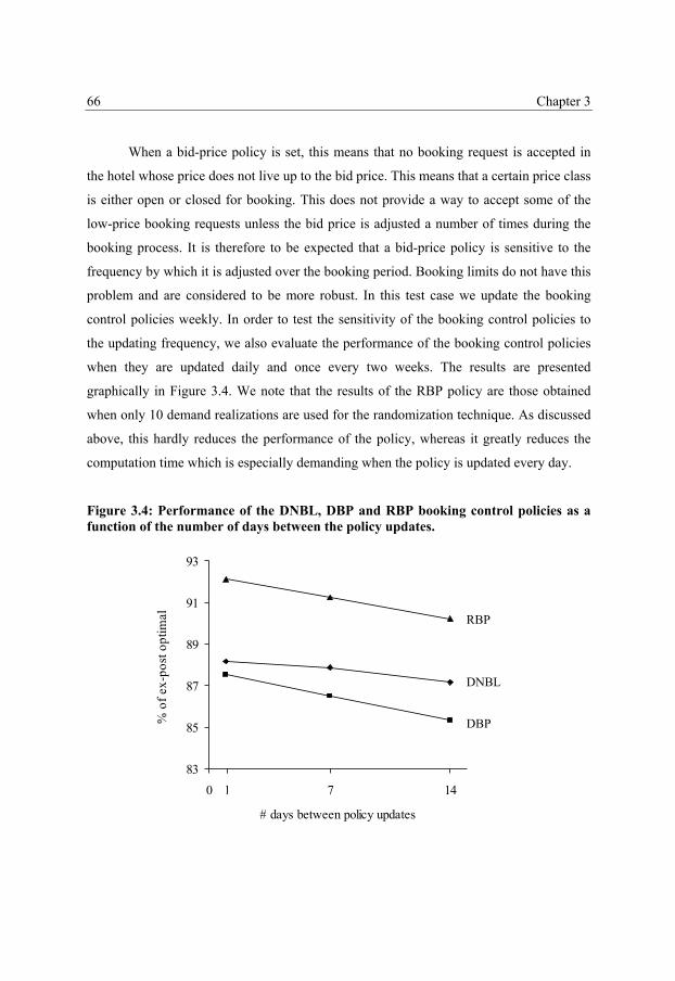
76
Chapter 3 66
When a bid-price policy is set, this means that no booking request is accepted in
the hotel whose price does not live up to the bid price. This means that a certain price class
is either open or closed for booking. This does not provide a way to accept some of the
low-price booking requests unless the bid price is adjusted a number of times during the
booking process. It is therefore to be expected that a bid-price policy is sensitive to the
frequency by which it is adjusted over the booking period. Booking limits do not have this
problem and are considered to be more robust. In this test case we update the booking
control policies weekly. In order to test the sensitivity of the booking control policies to
the updating frequency, we also evaluate the performance of the booking control policies
when they are updated daily and once every two weeks. The results are presented
graphically in Figure 3.4. We note that the results of the RBP policy are those obtained
when only 10 demand realizations are used for the randomization technique. As discussed
above, this hardly reduces the performance of the policy, whereas it greatly reduces the
computation time which is especially demanding when the policy is updated every day.
Figure 3.4: Performance of the DNBL, DBP and RBP booking control policies as a function of the number of days between the policy updates.
83
85
87
89
91
93
0 7 14
# days between policy updates
% o
f ex-
post
opt
imal
DNBL
DBP
RBP
1
77
Models and Techniques for Hotel Revenue Management using a Rolling Horizon 67
Figure 3.4 shows that the DBP and RBP policies are indeed more sensitive to the
frequency by which the policies are updated than the DNBL policy. This results from the
slope of the lines presented in Figure 3.4, which are steeper for the two bid-price polices.
This means that the difference between the performance of the DNBL and DBP policies is
reduced and between the DNBL and RBP policies is enlarged as the update frequency is
increased. When the booking control policies are updated once every two weeks, the
DNBL policy outperforms the DBP policy by 1.84% of the optimal revenue. When the
policies are updated once every week this is 1.39% and for every day this is only 0.61%.
The differences between the DNBL and RBP policies are 3.01%, 3.34% and 3.98% when
the days between the policy updates are reduced from 14 to 7 to 1 respectively. Note,
however, that although it is possible in practice to update a booking control policy on a
daily basis, e.g. during the night, it is hardly possible to do so more frequently. Our
findings show that the DNBL still outperforms the DBP policy when the policies are
updated daily.
3.6.2 Stochastic Booking Control Policies
The results presented in the previous section, show that it can be rewarding to take the
stochastic nature of demand into account when constructing a booking control policy.
Whereas the RBP policy needs a number of model optimizations, and therefore
computation time, to set its bid prices, the stochastic model given in (3.2) provides a way
to do so with only one optimization. However, before the model can be applied, the
manner by which the demand distribution is approximated has to be determined.
Based on the findings of de Boer et al (2002), who show that for the airline
industry 3 or 4 demand scenarios suffice to capture most of the extra revenue generated by
considering the stochastic nature of the demand, we consider only 3 demand scenarios for
the stochastic model. These demand scenarios can be interpreted as a low, an average and
a high demand scenario. We define the level of the average demand scenario as the
expected demand and define the levels of the low and high demand scenarios as k times

78
Chapter 3 68
the standard deviation away from the expected demand. For determining the scenario
probabilities, we define the variable:
j
jjj
Dz
σµ−
= , (3.5)
where Dj is the demand for booking type j and µj its mean and σj its standard deviation.
Then, by the central limit theorem, zj is approximately distributed as a standard normal
distribution. Now, because we can write jjj kD σµ +≥ as: kz j ≥ , we can approximate
the probability that the demand exceeds the average demand plus k times the standard
deviation by N(-k), where N(.) is the distribution function of the standard normal
distribution. This way we can easily obtain the scenario probabilities for each scenario
spread k.
In Figure 3.5 we show the performance of the SNBL and SBP policies for values
of scenario spreads ranging from k = 0.1 to k = 2. Note that when k = 2, the spread
between the low and high demand scenarios is large, since 9773.0)2Pr( =−≥ jjjD σµ
and 0227.0)2Pr( =+≥ jjjD σµ . The performance of the booking control policies is
measured with respect to the ex-post optimal revenue. Each evaluation point reflects the
average revenue obtained over the same 100 simulated booking processes used in the
previous section. We also include the average revenues obtained by the DNBL, DBP and
RBP policies in Figure 3.5. The full performance information for the SNBL and SBP
policies is provided in Table 3.4.
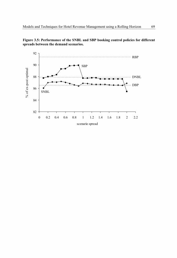
79
Models and Techniques for Hotel Revenue Management using a Rolling Horizon 69
Figure 3.5: Performance of the SNBL and SBP booking control policies for different spreads between the demand scenarios.
82
84
86
88
90
92
0 0.2 0.4 0.6 0.8 1 1.2 1.4 1.6 1.8 2 2.2
scenario spread
% o
f ex-
post
opt
imal
DNBL
DBP
RBP
SNBL
SBP
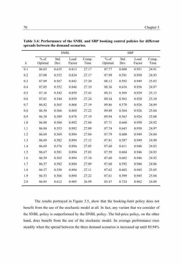
80
Chapter 3 70
Table 3.4: Performance of the SNBL and SBP booking control policies for different spreads between the demand scenarios.
SNBL SBP
% of Std. Load Comp. % of Std. Load Comp. k Optimal Dev. Factor Time Optimal Dev. Factor Time
0.1 86.03 0.635 0.813 27.17 87.77 0.608 0.951 24.91
0.2 87.00 0.552 0.834 27.17 87.99 0.591 0.950 24.93
0.3 87.09 0.567 0.842 27.20 88.12 0.592 0.949 25.03
0.4 87.05 0.552 0.846 27.19 88.36 0.616 0.936 24.97
0.5 87.18 0.542 0.859 27.43 89.31 0.569 0.929 25.13
0.6 87.01 0.544 0.859 27.24 89.34 0.563 0.928 25.10
0.7 86.82 0.565 0.868 27.19 89.86 0.578 0.926 24.89
0.8 86.58 0.566 0.869 27.22 89.89 0.564 0.926 25.04
0.9 86.38 0.589 0.878 27.19 89.94 0.563 0.926 25.08
1.0 86.88 0.560 0.892 27.04 87.71 0.660 0.950 24.92
1.1 86.84 0.553 0.892 27.09 87.74 0.643 0.950 24.97
1.2 86.69 0.569 0.894 27.04 87.79 0.600 0.949 24.84
1.3 86.69 0.582 0.894 27.12 87.81 0.587 0.949 24.90
1.4 86.69 0.576 0.894 27.05 87.60 0.611 0.946 24.83
1.5 86.67 0.581 0.894 27.03 87.59 0.604 0.946 24.83
1.6 86.59 0.565 0.894 27.10 87.60 0.602 0.946 24.92
1.7 86.57 0.582 0.894 27.09 87.60 0.592 0.946 24.86
1.8 86.57 0.550 0.894 27.11 87.62 0.602 0.945 25.05
1.9 86.53 0.566 0.894 27.22 87.61 0.599 0.945 25.04
2.0 86.85 0.612 0.905 26.99 85.47 0.724 0.962 24.88
The results portrayed in Figure 3.5, show that the booking-limit policy does not
benefit from the use of the stochastic model at all. In fact, any variant that we consider of
the SNBL policy is outperformed by the DNBL policy. The bid-price policy, on the other
hand, does benefit from the use of the stochastic model. Its average performance rises
steadily when the spread between the three demand scenarios is increased up until 89.94%
81
Models and Techniques for Hotel Revenue Management using a Rolling Horizon 71
of the optimal revenue for k = 0.9. If the demand spread is increased to 1, however, its
average performance falls back to 87.71%. When the scenario spread is increased to 2 the
performance of the SBP policy is even worse than for the DBP policy. This shows that the
SBP policy is very sensitive to the discretization of the demand chosen in the underlying
model. The SNBL policy does not seem to have this problem, since its performance is
relatively robust over the different scenario spreads that we consider. Except for k = 2, the
revenues obtained by the SNBL policy are, however, much less than the revenues obtained
by the SBP policy. Both policies are outperformed by the RBP policy. However, Table 3.4
shows that although the SNBL and SBP policies need about 2.5 times as much
computation time as the DNBL and SBP policies, they are still much faster than the RBP
policy.
The fact the booking-limit policy does not benefit from the use of the stochastic
model seems surprising but has been observed before for the airline industry by
Williamson (1992) and de Boer et al. (2002). They argue that this can mainly be ascribed
to the fact that the booking limits are nested. When the stochastic nature of demand is
taken into account explicitly, this often results in booking limits that are more protective
for the higher price classes. However, nesting is already a method to deal with additional
demand for these price classes, such that combining both methods quickly results in
overprotection of the higher price classes. We do observe an increase in the performance
of the bid-price policy when it is based on the stochastic model. This can be expected
since a bid-price policy does not make use of nesting techniques that can counter the
effects of the stochastic model. Williamson (1992) and de Boer et al. (2002) do not find
such positive results for the SBP policy. This can be due to the differences between the
network structure considered for the airline and hotel test cases. However, since the SBP
policy depends highly on the chosen demand discretization, one can also easily obtain
different performance observations for different model specifications.
82
Chapter 3 72
3.7 Summary and Conclusion
In this chapter, we study different booking control policies for the hotel revenue
management problem. The main difference that sets the hotel revenue management
problem apart from the airline problem, is that the combinatorial effects present in the
problem are not due to the multiple flights that are used by a passenger, but rather by the
overlap between the guests in the hotel that stay for multiple days. This overlap is not
restricted to a fixed time horizon. Therefore, we define a rolling horizon of decision
periods which conveniently captures the overlap between the different booking requests
for the hotel.
We consider five booking control policies that are applied over the rolling horizon
of decision periods. Bid prices and nested booking limits are constructed based on the
well-known deterministic mathematical programming model. Further, we also obtain bid
prices and nested booking limits based on a stochastic mathematical programming model
that has not been used for hotel revenue management before. Finally, randomized bid
prices are obtained by ways of simulation. The performance of the different booking
control policies is evaluated in a simulated environment. The results show that the
randomized bid prices strictly outperform all other policies and reach up to 91.33% of the
optimal revenue that can be obtained. However, this policy is also computationally very
demanding and therefore not always useful in practice. We show that in our test case the
number of demand realizations used for the randomization technique can be chosen as low
as 10 without sacrificing much of the performance and reliability of the policy. This is a
means to reduce the computation time of the policy.
When the booking limits and bid prices are obtained from the deterministic model,
the booking limits provide better results. However, since the bid prices are more sensitive
to the frequency by which the policy is updated, the gap between the performance of the
booking-limit and bid-price policies can be reduced when the policies are updated more
frequently. Nevertheless, the booking limits still provide better results when the policies
are updated every day. We show that the booking-limit policy does not benefit from the
use of the stochastic model. This is in line with prior findings by Williamson (1992) and
83
Models and Techniques for Hotel Revenue Management using a Rolling Horizon 73
de Boer et al. (2002) for the airline industry, and can be explained by the nested nature of
the policy which already accounts for the stochastic nature of demand in its own way. The
bid-price policy, on the other hand, can benefit greatly from the use of the stochastic
model. We show that the stochastic bid prices can outperform all other policies except for
the randomized bid prices. However, the stochastic bid prices are very sensitive to the
demand distribution considered in the underlying mathematical programming model. In
fact, when the demand discretization is not chosen beneficially, the stochastic bid prices
can perform very badly. The deterministic booking-limit policy does not have this
problem and even provides relatively robust results for different updating frequencies.
Therefore, the deterministic booking-limit policy still is one of the most attractive policies
to use in practice.
Following the results presented in this chapter, the stochastic mathematical
programming model seems an interesting object for further research. It would be
interesting to see whether insights can be obtained concerning the relation between the
demand discretization chosen in the model and the performance of the bid prices. Such
insights might take away some of the uncertainties involved with adapting the stochastic
bid-price policy for practical use. Further, research opportunities lie in extending the
booking control policies presented here to include aspects left out of this study, such as
overbooking and group bookings. From the airline revenue management literature we
know, however, that some aspects of the revenue management problem, such as
competition and buy-up behavior, can be particularly hard to incorporate into a model.
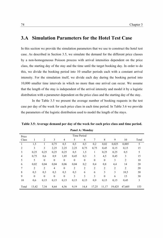
84
Chapter 3 74
3.A Simulation Parameters for the Hotel Test Case
In this section we provide the simulation parameters that we use to construct the hotel test
case. As described in Section 3.5, we simulate the demand for the different price classes
by a non-homogeneous Poisson process with arrival intensities dependent on the price
class, the starting day of the stay and the time until the target booking day. In order to do
this, we divide the booking period into 10 smaller periods each with a constant arrival
intensity. For the simulation itself, we divide each day during the booking period into
10,000 smaller time intervals in which no more than one arrival can occur. We assume
that the length of the stay is independent of the arrival intensity and model it by a logistic
distribution with a parameter dependent on the price class and the starting day of the stay.
In the Table 3.5 we present the average number of booking requests in the test
case per day of the week for each price class in each time period. In Table 3.6 we provide
the parameters of the logistic distribution used to model the length of the stays.
Table 3.5: Average demand per day of the week for each price class and time period.
Panel A: Monday
Price Time Period Class 1 2 3 4 5 6 7 8 9 10 Total 1 1,5 1 0,75 0,5 0,5 0,5 0,2 0,02 0,025 0,005 5 2 3 3 2,25 2,25 2,25 0,75 0,75 0,45 0,15 0,15 15 3 0,25 0,25 0,25 0,25 0,5 1,5 1 0,25 0,25 0,5 5 4 0,75 0,6 0,9 1,05 0,45 0,3 3 4,5 0,45 3 15 5 5 0 0 0 0 0 0 0 3 2 10 6 0,02 0,04 0,04 0,06 0,04 0,2 0,4 0,8 4,4 14 20 7 2 2 4 0 2 2 2 2 2 2 20 8 0,3 0,3 0,3 0,3 0,3 6 6 3 3 10,5 30 9 0 0 0 0 3 3 3 0 6 15 30 10 0,6 0,15 0,15 0,15 0,15 0,15 0,9 0,15 0,15 0,45 3
Total 13,42 7,34 8,64 4,56 9,19 14,4 17,25 11,17 19,425 47,605 153
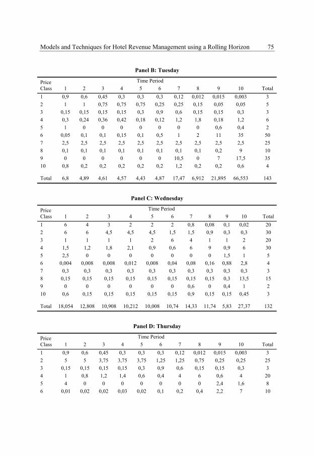
85
Models and Techniques for Hotel Revenue Management using a Rolling Horizon 75
Panel B: Tuesday
Price Time Period Class 1 2 3 4 5 6 7 8 9 10 Total 1 0,9 0,6 0,45 0,3 0,3 0,3 0,12 0,012 0,015 0,003 3 2 1 1 0,75 0,75 0,75 0,25 0,25 0,15 0,05 0,05 5 3 0,15 0,15 0,15 0,15 0,3 0,9 0,6 0,15 0,15 0,3 3 4 0,3 0,24 0,36 0,42 0,18 0,12 1,2 1,8 0,18 1,2 6 5 1 0 0 0 0 0 0 0 0,6 0,4 2 6 0,05 0,1 0,1 0,15 0,1 0,5 1 2 11 35 50 7 2,5 2,5 2,5 2,5 2,5 2,5 2,5 2,5 2,5 2,5 25 8 0,1 0,1 0,1 0,1 0,1 0,1 0,1 0,1 0,2 9 10 9 0 0 0 0 0 0 10,5 0 7 17,5 35 10 0,8 0,2 0,2 0,2 0,2 0,2 1,2 0,2 0,2 0,6 4
Total 6,8 4,89 4,61 4,57 4,43 4,87 17,47 6,912 21,895 66,553 143
Panel C: Wednesday
Price Time Period Class 1 2 3 4 5 6 7 8 9 10 Total 1 6 4 3 2 2 2 0,8 0,08 0,1 0,02 20 2 6 6 4,5 4,5 4,5 1,5 1,5 0,9 0,3 0,3 30 3 1 1 1 1 2 6 4 1 1 2 20 4 1,5 1,2 1,8 2,1 0,9 0,6 6 9 0,9 6 30 5 2,5 0 0 0 0 0 0 0 1,5 1 5 6 0,004 0,008 0,008 0,012 0,008 0,04 0,08 0,16 0,88 2,8 4 7 0,3 0,3 0,3 0,3 0,3 0,3 0,3 0,3 0,3 0,3 3 8 0,15 0,15 0,15 0,15 0,15 0,15 0,15 0,15 0,3 13,5 15 9 0 0 0 0 0 0 0,6 0 0,4 1 2 10 0,6 0,15 0,15 0,15 0,15 0,15 0,9 0,15 0,15 0,45 3
Total 18,054 12,808 10,908 10,212 10,008 10,74 14,33 11,74 5,83 27,37 132
Panel D: Thursday
Price Time Period Class 1 2 3 4 5 6 7 8 9 10 Total 1 0,9 0,6 0,45 0,3 0,3 0,3 0,12 0,012 0,015 0,003 3 2 5 5 3,75 3,75 3,75 1,25 1,25 0,75 0,25 0,25 25 3 0,15 0,15 0,15 0,15 0,3 0,9 0,6 0,15 0,15 0,3 3 4 1 0,8 1,2 1,4 0,6 0,4 4 6 0,6 4 20 5 4 0 0 0 0 0 0 0 2,4 1,6 8 6 0,01 0,02 0,02 0,03 0,02 0,1 0,2 0,4 2,2 7 10
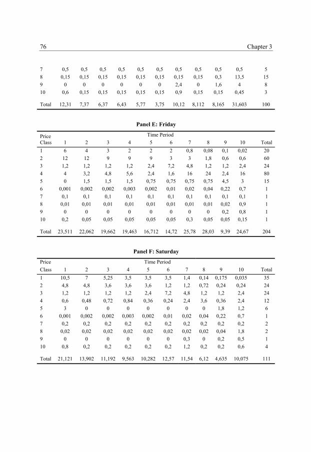
86
Chapter 3 76
7 0,5 0,5 0,5 0,5 0,5 0,5 0,5 0,5 0,5 0,5 5 8 0,15 0,15 0,15 0,15 0,15 0,15 0,15 0,15 0,3 13,5 15 9 0 0 0 0 0 0 2,4 0 1,6 4 8 10 0,6 0,15 0,15 0,15 0,15 0,15 0,9 0,15 0,15 0,45 3
Total 12,31 7,37 6,37 6,43 5,77 3,75 10,12 8,112 8,165 31,603 100
Panel E: Friday
Price Time Period Class 1 2 3 4 5 6 7 8 9 10 Total 1 6 4 3 2 2 2 0,8 0,08 0,1 0,02 20 2 12 12 9 9 9 3 3 1,8 0,6 0,6 60 3 1,2 1,2 1,2 1,2 2,4 7,2 4,8 1,2 1,2 2,4 24 4 4 3,2 4,8 5,6 2,4 1,6 16 24 2,4 16 80 5 0 1,5 1,5 1,5 0,75 0,75 0,75 0,75 4,5 3 15 6 0,001 0,002 0,002 0,003 0,002 0,01 0,02 0,04 0,22 0,7 1 7 0,1 0,1 0,1 0,1 0,1 0,1 0,1 0,1 0,1 0,1 1 8 0,01 0,01 0,01 0,01 0,01 0,01 0,01 0,01 0,02 0,9 1 9 0 0 0 0 0 0 0 0 0,2 0,8 1 10 0,2 0,05 0,05 0,05 0,05 0,05 0,3 0,05 0,05 0,15 1
Total 23,511 22,062 19,662 19,463 16,712 14,72 25,78 28,03 9,39 24,67 204
Panel F: Saturday
Price Time Period Class 1 2 3 4 5 6 7 8 9 10 Total 1 10,5 7 5,25 3,5 3,5 3,5 1,4 0,14 0,175 0,035 35 2 4,8 4,8 3,6 3,6 3,6 1,2 1,2 0,72 0,24 0,24 24 3 1,2 1,2 1,2 1,2 2,4 7,2 4,8 1,2 1,2 2,4 24 4 0,6 0,48 0,72 0,84 0,36 0,24 2,4 3,6 0,36 2,4 12 5 3 0 0 0 0 0 0 0 1,8 1,2 6 6 0,001 0,002 0,002 0,003 0,002 0,01 0,02 0,04 0,22 0,7 1 7 0,2 0,2 0,2 0,2 0,2 0,2 0,2 0,2 0,2 0,2 2 8 0,02 0,02 0,02 0,02 0,02 0,02 0,02 0,02 0,04 1,8 2 9 0 0 0 0 0 0 0,3 0 0,2 0,5 1 10 0,8 0,2 0,2 0,2 0,2 0,2 1,2 0,2 0,2 0,6 4
Total 21,121 13,902 11,192 9,563 10,282 12,57 11,54 6,12 4,635 10,075 111
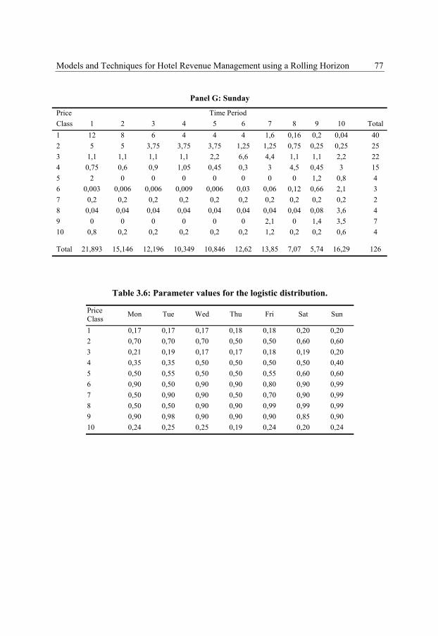
87
Models and Techniques for Hotel Revenue Management using a Rolling Horizon 77
Panel G: Sunday
Price Time Period Class 1 2 3 4 5 6 7 8 9 10 Total 1 12 8 6 4 4 4 1,6 0,16 0,2 0,04 40 2 5 5 3,75 3,75 3,75 1,25 1,25 0,75 0,25 0,25 25 3 1,1 1,1 1,1 1,1 2,2 6,6 4,4 1,1 1,1 2,2 22 4 0,75 0,6 0,9 1,05 0,45 0,3 3 4,5 0,45 3 15 5 2 0 0 0 0 0 0 0 1,2 0,8 4 6 0,003 0,006 0,006 0,009 0,006 0,03 0,06 0,12 0,66 2,1 3 7 0,2 0,2 0,2 0,2 0,2 0,2 0,2 0,2 0,2 0,2 2 8 0,04 0,04 0,04 0,04 0,04 0,04 0,04 0,04 0,08 3,6 4 9 0 0 0 0 0 0 2,1 0 1,4 3,5 7 10 0,8 0,2 0,2 0,2 0,2 0,2 1,2 0,2 0,2 0,6 4
Total 21,893 15,146 12,196 10,349 10,846 12,62 13,85 7,07 5,74 16,29 126
Table 3.6: Parameter values for the logistic distribution.
Price Class Mon Tue Wed Thu Fri Sat Sun
1 0,17 0,17 0,17 0,18 0,18 0,20 0,20 2 0,70 0,70 0,70 0,50 0,50 0,60 0,60 3 0,21 0,19 0,17 0,17 0,18 0,19 0,20 4 0,35 0,35 0,50 0,50 0,50 0,50 0,40 5 0,50 0,55 0,50 0,50 0,55 0,60 0,60 6 0,90 0,50 0,90 0,90 0,80 0,90 0,99 7 0,50 0,90 0,90 0,50 0,70 0,90 0,99 8 0,50 0,50 0,90 0,90 0,99 0,99 0,99 9 0,90 0,98 0,90 0,90 0,90 0,85 0,90 10 0,24 0,25 0,25 0,19 0,24 0,20 0,24

88

89
Chapter 4 Airline Revenue Management with Shifting Capacity
4.1 Introduction
Airline revenue management is the practice of controlling the booking requests that an
airline company receives such that the planes are filled with the most profitable
passengers. One of the essential assumptions in the traditional airline revenue
management problem is that the capacities of the flights are fixed and given. In this
chapter, we relax this assumption and extend the problem to include flexible capacities.
Traditionally, airlines determine the capacities of the flights well before the booking
process starts. However, making such capacity decisions dynamically during the booking
process has gained the interest of both academics as practitioners in recent years. For
example, Berge and Hopperstad (1993) and Listes and Dekker (2002) present methods to
apply the fleet assignment problem in a dynamic manner, which is known as demand-
driven-dispatch (D3). A method to assign capacity where it is needed in a less drastic
manner than swapping planes, is provided by the use of convertible seats. A row of these
seats can be converted from business class seats to economy class seats and vice versa.
This offers an airline company the possibility to adjust the capacity configuration within a
90
Chapter 4 80
plane, i.e. between the business and economy class sections, to the demand pattern at
hand. In this study, we show how to incorporate the shifting capacity opportunity offered
by the convertible seats into a dynamic, network-based revenue management model. We
also extend the model to include cancellations and overbooking. The revenue potential of
the shifting capacity opportunity is evaluated in a simulated environment.
In Section 4.2 we introduce the convertible seats and the shifting capacity
opportunity they provide. A mathematical formulation of the problem is given in Section
4.3. We first provide the formulation of the standard airline revenue management problem
and extend this for the shifting capacity decision and cancellations and overbooking. In
Section 4.4 we describe the test case that we construct to evaluate the revenue potential of
the various ways to deal with the shifting capacity opportunity. We present the
computational results of the test case in Section 4.4 and conclude this chapter in Section
4.5.
4.2 Shifting Capacity
In the traditional airline revenue management problem, the capacities of a plane and its
different sections, i.e. business and economy class, are considered to be fixed and given.
Despite of this, airline companies are not unfamiliar with the practice of shifting capacity
from the business to the economy class. This is done by ‘upgrading’ individual passengers
from economy to business or by ‘moving the curtain’ between the two sections. A
drawback of these procedures is that passengers that pay for the economy class get the
luxury of the business class (or at least a business class seat) for free. An airline company
should prevent this from happening on a large scale because of the danger that people will
anticipate on this and start booking economy class with the probability to be given a
business class seat instead of booking business class in the first place. Therefore,
upgrading and moving the curtain are not desirable tactics to apply on a large scale.
Another way for shifting business and economy class capacities is provided by so-
called convertible seats. By a simple procedure, a row of these seats can be converted

91
Airline Revenue Management with Shifting Capacity 81
from economy class to business class seats and vice versa. When a row is converted from
business to economy class, the number of seats in the row is increased and the width of
each seat is decreased. The distances between the rows, however, remain the same. An
example of this is given in Figure 4.1. In this figure, taken from the Swiss Air Lines 2002
Timetable, an Airbus 321 plane is shown equipped with convertible seats. Each row of
seats can be used as either six economy class seats or five business class seats. The table
included in Figure 4.1 gives a number of possible configurations of the plane varying from
no business class seats in configuration A to 76 business class seats in configuration Q.
Because a passenger that has booked for the economy class indeed gets an
economy class seat, the drawback previously mentioned for upgrading and moving the
curtain does not apply when the convertible seats are used. Moreover, extra seats become
available whenever a business class row is converted into an economy class row. The
convertible seats can be used without any serious consequences which makes the plane
very flexible in coping with different demand patterns. These different demand patterns
can occur among flights that are flown on different days of the week or on different times
of the day. Also seasonal differences can be encountered, as can differences caused by
unforeseen events such as a decline in demand during an economic regression.
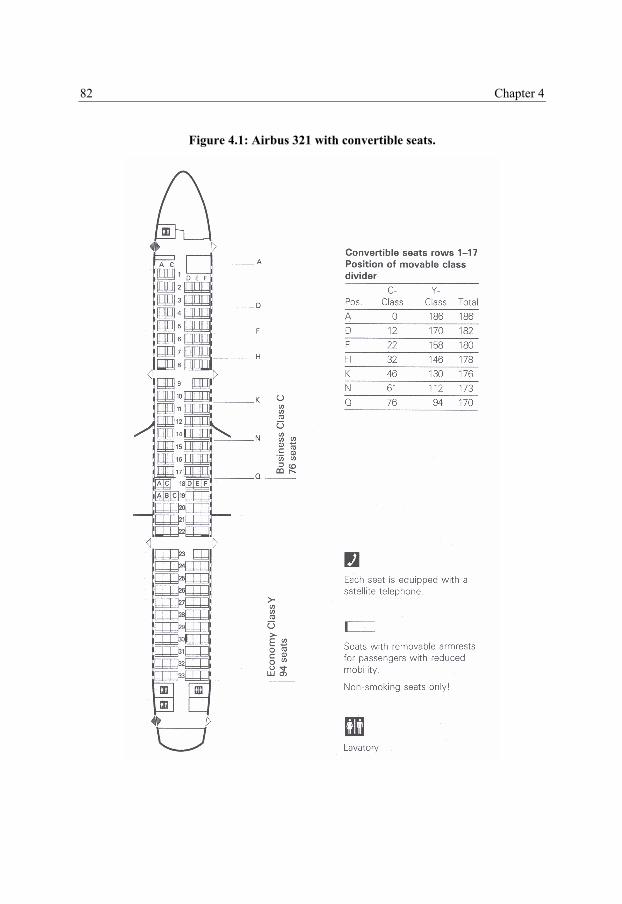
92
Chapter 4 82
Figure 4.1: Airbus 321 with convertible seats.

93
Airline Revenue Management with Shifting Capacity 83
In this chapter, we provide a model to incorporate the shifting capacity opportunity
offered by the convertible seats into the traditional revenue management problem. The
booking control policy that we use to extend for the shifting capacity decision is a
dynamic approximation scheme, which is re-optimized for every new booking request.
The underlying model is the standard deterministic mathematical programming model for
network revenue management. However, as Talluri and van Ryzin (1999), we extend the
model to account for the stochastic nature of demand by ways of simulation. A nice
additional property of the dynamic approximation scheme that we construct, is that it can
easily handle group bookings since it can just as easily compute the opportunity costs of
one as of multiple seats. Most other revenue management policies do not have this
property. On the other hand, we recognize that when a flight network is large, the
computation time involved with the dynamic approximation scheme often prevents it from
being useful for practical use. However, it still is an interesting and scarcely studied
solution method that can be useful for smaller problem instances. Additionally, it provides
a way to study the revenue potential of the shifting capacity opportunity with as little
interference as possible of the inefficiencies that the more common booking control
policies, such as booking limits and bid prices, generally cope with. We note that the
underlying mathematical programming model that we use also provides the means to
construct booking limits and bid prices in much the same way as the standard revenue
management models.
In our booking control policy, we allow for cancellations and overbooking in much
the same way as Bertsimas and Popescu (2003) do. Overbooking is not always
incorporated in revenue management research, but it is important to do so in combination
with the shifting capacity decision. When determining an overbooking policy, one should
take into account the fact that one booking can block an entire row of seats from becoming
available for the other section of the plane. Also, it is interesting to see if in some cases it
is profitable to deny one or two accepted bookings to board on the flight such that the row
becomes available for the other section, even though there are costs involved by doing so.
For illustration, we describe a test case in which one plane is used for a series of flights
and compare the results obtained in a simulated environment when the shifting capacity
94
Chapter 4 84
decision is made (i) beforehand and is kept fixed over all flights, (ii) before each flight,
and (iii) dynamically during the booking process of each flight.
Finally, we note that the shifting capacity opportunity that we discuss in this
chapter, is a way to allocate capacity where it is needed. In this respect this study is the
first step towards the integration of revenue management and dynamic capacity
management. In the airline industry dynamic capacity management is generally associated
with the fleet assignment problem, which is aimed at assigning the different types of
planes to the different flights such that revenues are maximized. When this is done
dynamically, i.e. when the fleet assignment is changed to match the actual demand when
departure time closes, this is also known as demand-driven dispatch (D3) (see: Berge and
Hopperstad (1993) and Listes and Dekker (2002)). By using planes equipped with
convertible seats, airline companies will be able to fine-tune the capacity allocation started
with the fleet assignment and will be able to match capacity and demand even better.
4.3 Problem Formulation
The essential decision to be made in airline revenue management is whether or not to
accept a booking request when it arrives. In order to make this decision, the direct revenue
gained by accepting the request has to be compared to the revenue that can be expected to
be gained from the seats it uses if the request is not accepted, i.e. the opportunity costs of
the seats. For determining the opportunity costs of the seats, it is important to have a good
estimation of the future demand for the various routes and price classes. Further, it should
be taken into account that a route requested by a customer can consist of multiple flights.
This means that different routes can make use of the same flights. Therefore, in order to
get a good approximation of the opportunity costs, the combinatorial effects of the whole
network of flights have to be considered.
We formulate the problem under the standard assumptions in airline revenue
management that the general price structure and the booking period are fixed and known.
Further, we also keep to the common assumption that demand is independent of the
95
Airline Revenue Management with Shifting Capacity 85
booking control policy used. However, unlike many other revenue management studies,
we do allow for group bookings and cancellations and overbooking. Most importantly, we
relax the assumption that the capacities of the business and economy sections of the plane
are fixed. Instead, we consider the capacity to be shifted between the two sections.
In Section 4.3.1 we give the traditional formulation for the network revenue
management problem. In sections 4.3.2 and 4.3.3 we extend the model for the shifting
capacity decision and cancellations and overbooking respectively.
4.3.1 Traditional Problem Formulation
In traditional airline revenue management, the business and economy sections of the plane
are considered to be distinct and fixed. This means that the different sections of the plane
do not have to be modelled explicitly, but can conceptually be seen as two different flights
in the network with distinct demand. We note that a booking request for a route/fare-class
combination explicitly belongs to a business or an economy price class. We model
demand as a sequence of booking requests over time and we measure time in discrete
intervals counting backwards, i.e. at time 0 the process ends. The problem formulation that
we use in this chapter is slightly different from the one used in Chapter 2. Considering the
fact that we refrain from a fixed capacity in the following sections, we no longer define
the state of the process by the remaining capacity, but by the number of accepted booking
requests instead.
Consider a flight network consisting of n route/fare-class combinations and 2m
flights, where m is the actual number of flights in the network which is multiplied by 2
when the business and economy sections are considered to be different flights. Let r = (r1,
r2, …, rn)T, u = (u1, u2, …, un)T and c = (c1, c2, …, c2m)T be the fares, accepted booking
requests and capacities of the various route/fare-class combinations and flights. Further,
define the matrix A = [aij], such that aij = 1 whenever route/fare-class combination j uses
flight i and aij = 0 otherwise. Define Vt(u) as the optimal expected revenue that can be
obtained with t time units to go and u booking requests already accepted and Rt = (Rt,1,
96
Chapter 4 86
Rt,2, …, Rt,n)T as a random vector for which Rt,j = rj if a request for class j occurs at time t,
and Rt,j = 0 otherwise. Finally, let x = (x1, x2, …, xn)T be the control variable denoting
whether to accept a class j request (xj = 1) or not (xj = 0). Then, x is restricted to the set
cxuAxu ≤+∈= )(:1,0)( ntX and the Bellman equation for the optimal expected
revenue function Vt(u), is given by:
⎥⎦⎤
⎢⎣⎡ ++= −∈
)(max)( 1T
)(xuxRu
ux ttXt VEVt
, (4.1)
with the boundary condition:
V0(u) = 0, ∀ u.
The optimal control policy can easily be obtained from (4.1) and says to accept a booking
request for route/price-class combination j, with t time units to go and u booking requests
already accepted, if and only if sufficient capacity is available and:
)()( 11 jttj VVr euu +−≥ −− , (4.2)
where ej is the jth column of a n×n identity matrix. The left hand side of (4.2) denotes the
direct revenue associated with the booking request, whereas the right hand side denotes
the estimated opportunity costs of the seats taken up by the booking request.
The optimal control policy given by (4.2) has been derived in some form or
another for both discrete as well as continuous time by a number of people, including
Bertsimas and Popescu (2003), Chen et al. (1998), Lautenbacher and Stidham (1999), Lee
and Hersh (1993), Liang (1999), Subramanian et al. (1999), Talluri and Van Ryzin (1998,
1999) and Van Slyke and Young (2000). The difficulty, however, is to approximate Vt(u).
Let D = (D1, D2, …, Dn)T be the demand of the various route/price-class combinations for
97
Airline Revenue Management with Shifting Capacity 87
the remaining time periods. Then if D is known, Vt(u) can be obtained from the following
mathematical programming model:
=)(utV max xr T (4.3)
s.t. cxuA ≤+ )(
Dx ≤≤0 integer,
where x = (x1, x2, ..., xn)T determines the number of booking requests that are accepted for
each route/price-class combination. The mathematical programming model in (4.3)
provides a linear system of equations that can be solved by standard IP optimization
techniques such as branch and bound.
In practice, D will not be known. One way to obtain an approximation for Vt(u) is
to replace D with its expected value. However, this does not take into account the
stochastic nature of demand. A stochastic model has been proposed by Wollmer (1986).
But this model is computationally intractable because of the large number of decision
variables. A reduced version of Wollmer’s model, which considers only a limited number
of discretization points for the demand distribution, is proposed by De Boer et al. (2002).
The simplest method to incorporate the stochastic nature of demand is probably proposed
by Talluri and Van Ryzin (1999). They simulate a sequence of demand realizations and
compute the optimal future revenue for each of these realizations by the model given in
(4.3). They approximate Vt(u) by averaging the outcomes.
It is common practice to construct booking-limit or bid-price policies based on a
mathematical programming model as provided above. Such booking control policies can
be used for the on-line accept/deny decisions for a longer period of time until the policies
are updated. In this study, however, we do not make use of such a policy to bridge the
time between model optimizations. Instead we use a dynamic approximation scheme that
directly obtains an approximation of Vt(u) by optimizing the mathematical programming
model for every booking request that comes in. Such a dynamic approximation scheme
will not always be useful in practice, unless the problem instance is small. However, it is
98
Chapter 4 88
an interesting and scarcely studied method which provides us the means to study the
revenue potential of the shifting capacity opportunity without interference caused by the
booking control policy that is used.
An additional advantage of the dynamic approximation scheme is that it can deal
with group bookings in a natural way. Note that when a booking request is made for k
seats on route/price-class combination j, with t time units to go and u booking requests
already accepted, it should be accepted if and only if sufficient capacity is available and:
)()( 11 jttj kVVkr euu +−≥ −− . (4.4)
This is a natural extension of the optimal decision rule presented in (4.2). Most booking
control policies have difficulties with decisions concerning multiple units of capacity at
once, since they are based on small deviations of the value function. These small
deviations are often estimated by the dual prices of the underlying mathematical
programming model. The dynamic approximation scheme, on the other hand, can just as
easily approximate )(1 jt kV eu +− as )(1 jtV eu +− .
4.3.2 Problem Formulation with Shifting Capacity
In this section we extend the standard airline revenue management problem with the
shifting capacity decision. We use the same notation as in the previous section with the
difference that the capacity c is no longer a constant, but is now dependent on the shifting
capacity decision. We note that the optimal acceptance policy does not change, but the
underlying mathematical programming model does. Assume that each plane has got a
limited number of possible capacity configurations collected in the state space Y. Let m be
the number of flights and y = (y1, y2, ..., ym)T ∈ Y be the shifting capacity vector which
denotes the chosen capacity configuration for each plane. Further, let the capacities be

99
Airline Revenue Management with Shifting Capacity 89
defined as a function of y, c(y). Then, for a given demand vector D, Vt(u) can be obtained
by:
=)(utV max xr T (4.5)
s.t. )()( ycxuA ≤+
Dx ≤≤0 integer,
Y∈y ,
where x determines the number of requests accepted for each route/price-class
combination and y determines the capacity configurations of the planes.
Unless c(y) and Y are of a very specific form, model (4.5) will not be a system of
linear equations. Therefore, it can be very hard to optimize the model. However, we show
that the specifications of c(y) and Y that can be encountered in practice, are such that
model (4.5) generally reduces to a system of linear equations. In order to see this, we
describe the situation of a plane that has got two sections; a business and an economy
class section. Then a plane which is equipped with convertible seats usually has a number
of seats which are fixed for both sections along with a number of rows which can be used
as either business or economy class rows. Assume that the fixed seat capacity for the
business class is given by cb and for the economy class by ce. Further, let there be R rows
of convertible seats which can each be used for either bb business class seats or be
economy class seats. Then we can define:
⎟⎠⎞⎜
⎝⎛
−++= )()( yRbc
ybcyee
bbc , with RyyY ≤≤∈= 0:N .
In this case, y denotes the number of convertible rows appointed to the business class
section. Note that when we consider multiple flights, the capacity configurations of the
flights will have to be denoted by a vector y instead of only a number y.
100
Chapter 4 90
In order to present the model (4.5) with this specific formulation of c(y), we let cb,
ce, bb, be and R be vectors of dimension m×1, such that they contain the shifting capacity
information for all flights in the network. Further, we also partition n, r, x, A, u and D into
a part that contains the information concerning the business class and a part that contains
the information concerning the economy class. Then we can define:
=)(utV max eebb xrxr TT + (4.6)
s.t. bbbbb cybxuA ≤−+ T)(
eeeee cyRbxuA ≤−++ )()( T
bb Dx ≤≤0 integer,
ee Dx ≤≤0 integer,
Ry ≤≤0 integer,
where xb and xe determine the number of requests accepted for each route/price-class
combination in the business and economy class and y determines the configurations of the
planes. Model (4.6) consists of a linear system of equations and can therefore be
optimized by the same procedures as model (4.3). Furthermore, the model has the same
number of capacity constraints as model (4.3) and only has m more decision variables,
where m is the number of flights in the flight network. Note that, although model (4.6)
provides a configuration of the planes for every time it is optimized, only at the end of the
booking period, at time 0, the planes will be physically converted into the desirable
configuration.
4.3.3 Problem Formulation with Cancellations and Overbooking
In the airline industry, a large amount of bookings typically get cancelled before
departure. Therefore, in order to prevent the planes from taking off with empty seats,
airline companies overbook the flights. Whenever overbooking is applied, there is a
101
Airline Revenue Management with Shifting Capacity 91
probability that not all bookings can get on the plane. This can happen intentionally when
a low fare booking is denied boarding in favour of a high fare booking, or accidentally
when the number of cancellations is overestimated. However, there will be a penalty cost
involved with denying an accepted booking to board. These can consist of all kinds of
costs such as accommodation costs or loss of goodwill. The penalty costs normally
prevent airline companies from taking too much risk with overbooking. It is interesting to
see, however, if it is worthwhile to take more risk of bearing the costs of a denied
boarding if this means that the entire row is shifted from the economy to the business class
section of the plane or vice versa.
A deviation from the formulation before is that we define the variables x , u and
D as the net values of x, u and D, where we define the net value as the number of
booking requests corrected for the number of cancellations. This means that, if 30 booking
requests have been accepted for route/price-class combination j, of which 6 will be
cancelled in the future, then u = 30 but u = 24. Obviously it is not known in advance
which bookings will be cancelled. However, we can substitute u and D by expected or
simulated values. Finally, let qb = (qb,1, qb,2, …, bnbq , )T and qe = (qe,1, qe,2, …,
eneq , )T
denote the penalty costs of each route/price-class combination in the business and
economy class sections. Then, we define the following mathematical programming model
to obtain Vt(u) when cancellations and overbooking are taken into account:
=)(utV max eebbeebb zqzqxrxr TTTT −−+ (4.7)
s.t. bbbbbb cybzxuA ≤−−+ T)(
eeeeee cyRbzxuA ≤−+−+ )()( T
bb Dx ≤≤0 integer,
ee Dx ≤≤0 integer,
Ry ≤≤0 integer,
bz≤0 integer,
ez≤0 integer,

102
Chapter 4 92
where zb and ze determine which bookings in the business and economy class sections are
denied boarding when the plane takes off.
4.4 Description of the Test Case
In order to evaluate what the added value can be of using a revenue management policy
that exploits the shifting capacity opportunity offered by the convertible seats, we apply
the models presented in the previous section to a simulated test case. In this section we
discuss the simulation environment. The simulation environment that we construct is
chosen to reflect insights obtained from professionals in the airline industry. This means
that the results that we obtain in this specific setting give an indication of what one can
expect to find in practice.
The test case consists of a single flight that is flown three times by the same plane.
Each flight is characterized by its own typical demand pattern. These three flights can be
interpreted to be the same flight in different seasons, on different days of the week, or on
different times of the day. Specifically, we model one base flight together with one flight
that has more business class and less economy class passengers, and one flight that has
less business and more economy class passengers. The plane that is used for this test case
has a total of 35 rows of passenger seats that can all be used for either five business class
seats or six economy class seats. This resembles the Airbus 321 depicted in Figure 4.1
very much. We consider two price classes in the business class and four in the economy
class. The prices are given in Table 4.1. Also given in Table 4.1 is the average demand of
each price class for all three flights. Flight 2 is the base flight. For the first flight, the
average business class demand is defined as 30% above the business class demand on the
base flight, and the average economy class demand is defined as 30% below the average
economy class demand on the base flight. For the third flight this is the other way around.

103
Airline Revenue Management with Shifting Capacity 93
Table 4.1: Price classes.
Average Demand
Class Class Type Price Flight 1 Flight 2 Flight 3
1 Business $ 400 14.3 11 7.7
2 Business $ 350 36.4 28 19.6
3 Economy $ 250 22.4 32 41.6
4 Economy $ 200 30.8 44 57.2
5 Economy $ 150 51.1 73 94.9
6 Economy $ 100 43.4 62 80.6
Next to the fact that the six price classes differ in price and demand level, they also
have a specific booking pattern. The arriving booking requests are modelled by a non-
homogeneous Poisson process. This is done by partitioning the booking period into ten
smaller time periods each with a constant arrival rate. Demand for the two business classes
is assumed to realize at the end of the booking period, whereas demand for the two
cheapest price classes is modelled to occur at the beginning of the booking period.
Graphical presentations of the arrival patterns of the price classes for the base flight are
included in Figure 4.2. For the other two flights, the booking patterns are the same only
with different demand levels. For sake of simplicity, we do not model booking requests
for multiple seats, but only consider single seat bookings.
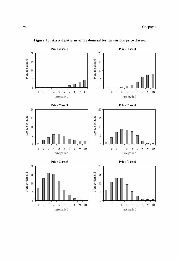
104
Chapter 4 94
Figure 4.2: Arrival patterns of the demand for the various price classes.
Price Class 1
0
5
10
15
20
1 2 3 4 5 6 7 8 9 10time period
aver
age
dem
and
Price Class 2
0
5
10
15
20
1 2 3 4 5 6 7 8 9 10time period
aver
age
dem
and
Price Class 3
0
5
10
15
20
1 2 3 4 5 6 7 8 9 10time period
aver
age
dem
and
Price Class 4
0
5
10
15
20
1 2 3 4 5 6 7 8 9 10time period
aver
age
dem
and
Price Class 5
0
5
10
15
20
1 2 3 4 5 6 7 8 9 10time period
aver
age
dem
and
Price Class 6
0
5
10
15
20
1 2 3 4 5 6 7 8 9 10time period
aver
age
dem
and
105
Airline Revenue Management with Shifting Capacity 95
When we consider cancellations and overbooking, we model each booking request
to have a probability that it will be cancelled. This cancellation probability is dependent on
the price class of the booking request and is the overall probability that the request is
cancelled somewhere between the time of booking and the end of the booking period. We
assume the cancellation probability to be homogeneous over time, such that a booking
request that is made t time periods before the end of the booking period and that has
cancellation probability p, has a cancellation probability per time unit of p/t. This way, we
are able to model the cancellations by a homogeneous Poisson process. We model the two
business classes to have a cancellation probability of 10%, the first two economy classes
of 12.5% and the two cheapest price classes of 15%. The simulated demand is increased
proportionally to these percentages in order to keep the net demand on the same level as in
the previous section.
As discussed in Section 4.3.3, the penalty costs of denying an accepted booking to
board have to be taken into account when overbooking is allowed. We set the penalty
costs at $500 for all price classes. This is more than the maximum revenue that can be
obtained from any price class, which means that it is never profitable to accept an extra
high price booking if this means that another booking has to be denied boarding. With the
shifting capacity opportunity, however, it can be profitable to deny one or two bookings to
board if this makes the entire row available for the other section of the plane. In
conclusion, we summarize the aspects that define the simulation environment in Table 4.2.

106
Chapter 4 96
Table 4.2: Specification of the test case.
3 consecutive flights with different demand levels
1 plane
35 convertible rows
5 business / 6 economy class seats per row
2 business / 4 economy price classes
different booking patterns for the different price classes
different cancellation probabilities for the different price classes
Overbooking is allowed
$500 penalty costs for a denied boarding
demand is independent of the booking control policies
no group bookings
4.5 Computational Results
In this section we present computational results in order to show how the models
described in the Section 4.3 can be used and what the added value can be of using a
revenue management policy that exploits the shifting capacity opportunity offered by the
convertible seats. We do this by evaluating the performance of three different booking
control policies to the simulated test case discussed in Section 4.4. The first booking
control policy does not make use of the fact that the capacity can be shifted between the
business and economy class sections, the second does, but only before the start of the
booking period, and the third fully integrates the revenue management and shifting
capacity decisions. The computational results when cancellations and overbooking are not
allowed are presented in Section 4.5.1. In Section 4.5.2 we present the results when
cancellations and overbooking are allowed.
107
Airline Revenue Management with Shifting Capacity 97
4.5.1 Results without Cancellations and Overbooking
We compare the performance of three different revenue management policies that differ in
the manner in which they deal with the shifting capacity opportunity. All three policies are
dynamic approximation schemes in the sense that the opportunity costs are estimated
anew for every booking request that comes in. The first policy does not incorporate the
shifting capacity decision into the accept/deny decision. For this policy, the capacity
remains fixed over all three flights and the traditional model presented in (4.3) is used to
estimate the opportunity costs. The capacity configuration of the plane is fixed at the
configuration obtained when model (4.6) is used to optimize all three flights at once based
on their expected demand. This is done before the booking period, and thus the revenue
management process, starts. We call this policy the Fixed Capacity (FC) policy. The
second policy does make use of the shifting capacity opportunity. For each flight, which
has its own specific demand pattern, a new capacity configuration is determined for the
plane. However, this configuration is not changed during the booking period. Before the
booking period starts, model (4.6) is used to determine the capacity configuration based on
the expected demand and during the booking period, model (4.3) is used to estimate the
opportunity costs. The third policy makes use of the shifting capacity opportunity
dynamically. It fully integrates the shifting capacity and revenue management problems
and continually uses model (4.6) to estimate the opportunity costs. This means that the
actual configuration of the plane will be known only at the end of the booking period. We
refer to the second policy as the Shifting Capacity (SC) policy and the third policy as the
Dynamic Shifting Capacity (DSC) policy.
All three policies are dynamic approximation schemes. We apply them in two
different ways that differ in the manner that the stochastic nature of demand is accounted
for. We distinguish the Deterministic Dynamic Approximation Scheme (DDAS) and the
Randomized Dynamic Approximation Scheme (RDAS). For the DDAS the opportunity
costs are approximated based on the expected future demand. That is, in the underlying
mathematical programming model, either model (4.3) or (4.6), the demand vector is
replaced by its expectation. For the RDAS a number of future demand realizations are

108
Chapter 4 98
simulated. For each demand realization the opportunity costs are determined and the
estimation of the opportunity costs that is used by the policy is defined as the average
opportunity costs over all simulations. The RDAS accounts for the stochastic nature of
demand, whereas the DDAS does not. However, the computation time involved with the
RDAS increases proportionally with the number of demand realizations that are
considered. Therefore, we restrict ourselves to 10 demand realizations for each
opportunity costs approximation. This is only a small number of realizations and we
suggest using more in practice in order to add reliability to the method. However, in the
test case provided in Chapter 3 we have seen that taking more than 10 demand realizations
for the randomization hardly increased the average performance and robustness of the
randomized policy. Although this is a different test case, we continue to use 10 demand
realizations for the randomization technique in order to reduce the computation time.
Combining the DDAS and RDAS with the FC, SC and DSC policies, gives us a
total of six booking control policies. In order to test the policies, we simulate 100
complete booking processes for all three flights. In Table 4.3 we report the overall
performance of the six booking control policies when they are applied to the 100
simulated booking processes. We also give the optimal revenues that can be determined
with hindsight for each simulation. The results are generated on a Pentium III 550 MHz
personal computer (256 MB RAM), using CPlex 7.1 to optimize the mathematical
programming models. All computation times are measured in seconds.

109
Airline Revenue Management with Shifting Capacity 99
Table 4.3: Performance of the booking control policies without cancellations and overbooking.
DDAS RDAS Ex-post FC SC DSC FC SC DSC Optimal
Revenue
Average 121470 124957 125114 121688 125197 126032 128258
Std. Dev. 3422 2873 2976 3479 3037 3048 3444
Minimum 113050 118550 118250 113150 118500 118500 120050
Maximum 129950 130200 130800 130100 131100 131700 136250
% of Ex-post Optimal
Average 94.78 97.49 97.60 94.95 97.67 98.30 100
Std. Dev. 1.393 1.107 0.783 1.339 1.120 0.751 0
Minimum 89.28 93.94 95.42 89.59 94.13 96.25 100
Maximum 98.22 99.58 99.57 98.34 99.77 99.74 100
Average Comp. Time (sec.) 3.85 3.75 6.58 37.24 34.82 62.50 -
Table 4.3 shows that the FC policies that do not take into account the shifting
capacity opportunity are clearly outperformed by the SC and DSC policies that do exploit
the shifting capacity opportunity. The FC policy obtains 94.78% and 94.95% of the
optimal revenue that can be generated when it is applied as DDAS and RDAS
respectively. This is a gap of 2.71% and 2.72% of the optimal revenue with the SC policy
when it is applied as DDAS and RDAS. The DSC, which is the most sophisticated policy,
performs best and reaches up to 97.6% and 98.3% of the optimal revenue. In our small test
case this means that the FC policies are outperformed by some $1162-$1448 per flight by
the policies that account for the shifting capacity opportunity. As these flights can be
flown one or even multiple times a day, and seeing that the extra revenues can be even
more for bigger planes, this can lead to a substantial gain in revenues for the airline
company. Whereas the FC policies are outperformed by the SC policies by 2.71% and
110
Chapter 4 100
2.72% of the optimal revenue, the DSC only performs 0.11% and 0.63% better than the
SC policies. In fact, all four policies that account for the shifting capacity opportunity
perform within 0.81% of each other. This shows that most of the revenue potential offered
by the convertible seats can be captured by adjusting the capacity configuration once for
each flight. Adjusting it dynamically, i.e. continuously during the booking process, only
creates a marginal improvement in the performance of the policy. However, doing so does
increase the computation time with some 75%-80%.
When focusing on the differences between the DDAS and RDAS results, Table 4.3
shows that the FC and SC policies do not seem to benefit much from the randomization
technique. The improvement in the performance of the FC and SC policies is 0.17% and
0.18% of the optimal revenue respectively. These improvements seem hardly worthwhile
if we consider the fact that the computation time of the RDAS is 10 times the computation
time of the DDAS. And this difference in computation time grows proportionally with the
number of demand realizations that are used for the randomization technique. The DSC
policy benefits more from the randomization. This can be explained from the fact that the
additional decisions it makes concerning the capacity configuration of the plane benefit
from the additional information provided by the randomization technique about the
demand distribution. However, also for the DSC policy, the average performance is only
increased by 0.70% of the optimal revenue. The standard deviations of the RDAS results
are not larger than those of the DDAS results, which indicates that the RDAS is not less
reliable than the DDAS when only 10 demand randomizations are used.
We use t-tests to test the statistical significance of the differences in the
performance of the booking control policies. The hypothesis that the difference in the
average performance of two booking control policies is equal to 0, is rejected for all policy
combinations with a p-value of 0.000 except when the DDAS/DSC and the RDAS/SC
methods are compared. This case results in a p-value of 0.428. We also apply a sign test
which counts the number of times a policy outperforms another policy and tests whether
this corresponds to a Binomial distribution with parameter 0.5. Also this test rejects the
hypothesis with a p-value of 0.000 for almost all cases. The only exceptions occur when
the DDAS/SC, DDAS/DSC and RDAS/SC methods are compared.
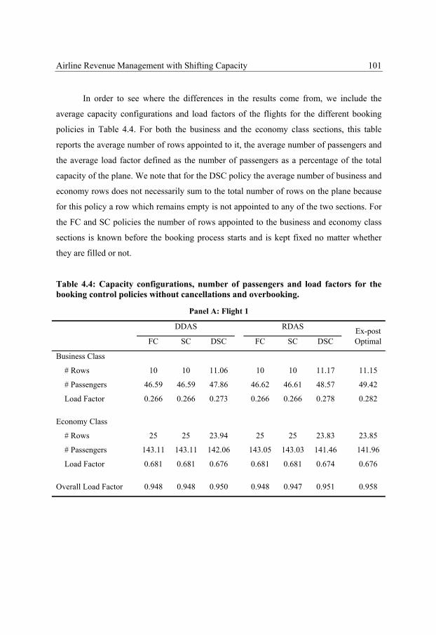
111
Airline Revenue Management with Shifting Capacity 101
In order to see where the differences in the results come from, we include the
average capacity configurations and load factors of the flights for the different booking
policies in Table 4.4. For both the business and the economy class sections, this table
reports the average number of rows appointed to it, the average number of passengers and
the average load factor defined as the number of passengers as a percentage of the total
capacity of the plane. We note that for the DSC policy the average number of business and
economy rows does not necessarily sum to the total number of rows on the plane because
for this policy a row which remains empty is not appointed to any of the two sections. For
the FC and SC policies the number of rows appointed to the business and economy class
sections is known before the booking process starts and is kept fixed no matter whether
they are filled or not.
Table 4.4: Capacity configurations, number of passengers and load factors for the booking control policies without cancellations and overbooking.
Panel A: Flight 1
DDAS RDAS Ex-post FC SC DSC FC SC DSC Optimal
Business Class
# Rows 10 10 11.06 10 10 11.17 11.15
# Passengers 46.59 46.59 47.86 46.62 46.61 48.57 49.42
Load Factor 0.266 0.266 0.273 0.266 0.266 0.278 0.282
Economy Class
# Rows 25 25 23.94 25 25 23.83 23.85
# Passengers 143.11 143.11 142.06 143.05 143.03 141.46 141.96
Load Factor 0.681 0.681 0.676 0.681 0.681 0.674 0.676
Overall Load Factor 0.948 0.948 0.950 0.948 0.947 0.951 0.958

112
Chapter 4 102
Panel B: Flight 2
DDAS RDAS Ex-post FC SC DSC FC SC DSC Optimal
Business Class
# Rows 10 8 7.79 10 8 8.01 8.13
# Passengers 39.70 37.65 37.18 39.69 37.69 38.23 39.55
Load Factor 0.227 0.215 0.212 0.227 0.215 0.218 0.226
Economy Class
# Rows 25 27 27.21 25 27 26.99 26.87
# Passengers 149.10 161.09 162.00 148.73 160.52 160.92 161.22
Load Factor 0.710 0.767 0.771 0.708 0.764 0.766 0.768
Overall Load Factor 0.937 0.982 0.984 0.935 0.980 0.985 0.994
Panel C: Flight 3
DDAS RDAS Ex-post FC SC DSC FC SC DSC Optimal
Business Class
# Rows 10 5 5.24 10 5 5.56 5.76
# Passengers 28.71 24.41 25.17 28.71 24.43 26.79 28.15
Load Factor 0.164 0.139 0.144 0.164 0.140 0.153 0.161
Economy Class
# Rows 25 30 29.76 25 30 29.44 29.24
# Passengers 149.59 179.43 177.42 149.41 179.30 175.62 175.44
Load Factor 0.712 0.854 0.845 0.711 0.854 0.836 0.835
Overall Load Factor 0.876 0.994 0.989 0.876 0.993 0.989 0.996
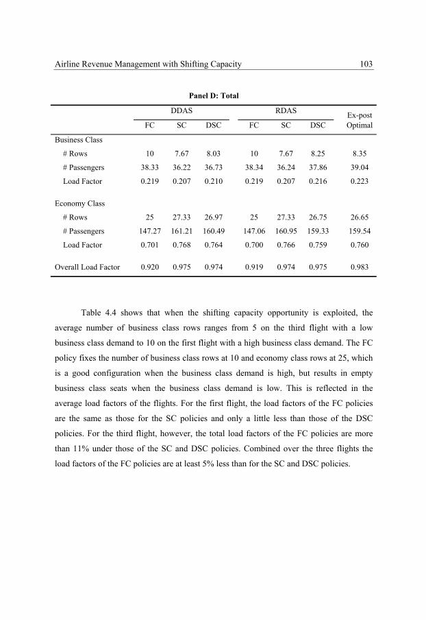
113
Airline Revenue Management with Shifting Capacity 103
Panel D: Total
DDAS RDAS Ex-post FC SC DSC FC SC DSC Optimal
Business Class
# Rows 10 7.67 8.03 10 7.67 8.25 8.35
# Passengers 38.33 36.22 36.73 38.34 36.24 37.86 39.04
Load Factor 0.219 0.207 0.210 0.219 0.207 0.216 0.223
Economy Class
# Rows 25 27.33 26.97 25 27.33 26.75 26.65
# Passengers 147.27 161.21 160.49 147.06 160.95 159.33 159.54
Load Factor 0.701 0.768 0.764 0.700 0.766 0.759 0.760
Overall Load Factor 0.920 0.975 0.974 0.919 0.974 0.975 0.983
Table 4.4 shows that when the shifting capacity opportunity is exploited, the
average number of business class rows ranges from 5 on the third flight with a low
business class demand to 10 on the first flight with a high business class demand. The FC
policy fixes the number of business class rows at 10 and economy class rows at 25, which
is a good configuration when the business class demand is high, but results in empty
business class seats when the business class demand is low. This is reflected in the
average load factors of the flights. For the first flight, the load factors of the FC policies
are the same as those for the SC policies and only a little less than those of the DSC
policies. For the third flight, however, the total load factors of the FC policies are more
than 11% under those of the SC and DSC policies. Combined over the three flights the
load factors of the FC policies are at least 5% less than for the SC and DSC policies.
114
Chapter 4 104
4.5.2 Results with Cancellations and Overbooking
In this section we present computational results when cancellations and overbooking are
included in the test case. We model the cancellation probability of a booking request by a
homogeneous Poisson process. The two business classes have a cancellation probability of
10%, the first two economy classes of 12.5% and the two cheapest price classes of 15%.
The simulated demand is increased proportionally to these percentages in order to keep the
net demand on the same level as in the previous section. The penalty costs of denying an
accepted booking to board is set at $500 for all price classes. This is more than the
maximum revenue that can be obtained from any price class, which means that it is never
profitable to accept an extra high price booking if this means that another booking has to
be denied boarding. However, with the shifting capacity opportunity it can be profitable to
deny one or two bookings to board if this makes the entire row available for the other
section of the plane.
We simulate 100 booking processes to which we apply the same six booking
control policies as in the previous section. The underlying mathematical programming
models are now adjusted to include cancellations and overbooking as described in Section
4.3.3. The overall performance of the six policies and the optimal results that can be
determined with hindsight are presented in Table 4.5.
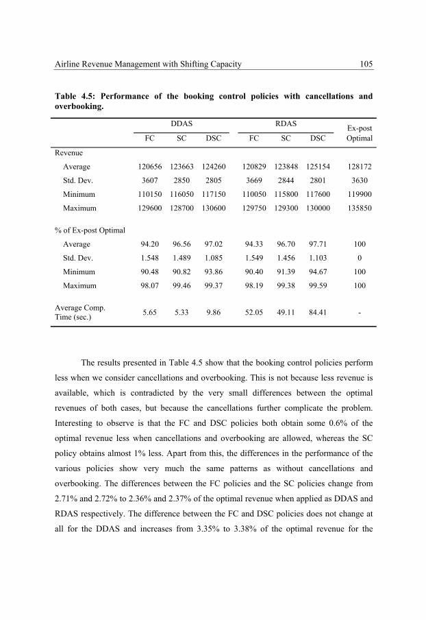
115
Airline Revenue Management with Shifting Capacity 105
Table 4.5: Performance of the booking control policies with cancellations and overbooking.
DDAS RDAS Ex-post FC SC DSC FC SC DSC Optimal
Revenue
Average 120656 123663 124260 120829 123848 125154 128172
Std. Dev. 3607 2850 2805 3669 2844 2801 3630
Minimum 110150 116050 117150 110050 115800 117600 119900
Maximum 129600 128700 130600 129750 129300 130000 135850
% of Ex-post Optimal
Average 94.20 96.56 97.02 94.33 96.70 97.71 100
Std. Dev. 1.548 1.489 1.085 1.549 1.456 1.103 0
Minimum 90.48 90.82 93.86 90.40 91.39 94.67 100
Maximum 98.07 99.46 99.37 98.19 99.38 99.59 100
Average Comp. Time (sec.) 5.65 5.33 9.86 52.05 49.11 84.41 -
The results presented in Table 4.5 show that the booking control policies perform
less when we consider cancellations and overbooking. This is not because less revenue is
available, which is contradicted by the very small differences between the optimal
revenues of both cases, but because the cancellations further complicate the problem.
Interesting to observe is that the FC and DSC policies both obtain some 0.6% of the
optimal revenue less when cancellations and overbooking are allowed, whereas the SC
policy obtains almost 1% less. Apart from this, the differences in the performance of the
various policies show very much the same patterns as without cancellations and
overbooking. The differences between the FC policies and the SC policies change from
2.71% and 2.72% to 2.36% and 2.37% of the optimal revenue when applied as DDAS and
RDAS respectively. The difference between the FC and DSC policies does not change at
all for the DDAS and increases from 3.35% to 3.38% of the optimal revenue for the
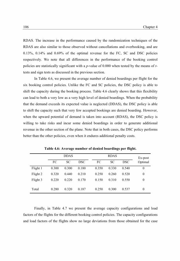
116
Chapter 4 106
RDAS. The increase in the performance caused by the randomization techniques of the
RDAS are also similar to those observed without cancellations and overbooking, and are
0.13%, 0.14% and 0.69% of the optimal revenue for the FC, SC and DSC policies
respectively. We note that all differences in the performance of the booking control
policies are statistically significant with a p-value of 0.000 when tested by the means of t-
tests and sign tests as discussed in the previous section.
In Table 4.6, we present the average number of denied boardings per flight for the
six booking control policies. Unlike the FC and SC policies, the DSC policy is able to
shift the capacity during the booking process. Table 4.6 clearly shows that this flexibility
can lead to both a very low as a very high level of denied boardings. When the probability
that the demand exceeds its expected value is neglected (DDAS), the DSC policy is able
to shift the capacity such that very few accepted bookings are denied boarding. However,
when the upward potential of demand is taken into account (RDAS), the DSC policy is
willing to take risks and incur some denied boardings in order to generate additional
revenue in the other section of the plane. Note that in both cases, the DSC policy performs
better than the other policies, even when it endures additional penalty costs.
Table 4.6: Average number of denied boardings per flight.
DDAS RDAS Ex-post FC SC DSC FC SC DSC Optimal
Flight 1 0.300 0.300 0.180 0.350 0.330 0.540 0
Flight 2 0.320 0.440 0.210 0.250 0.260 0.520 0
Flight 3 0.220 0.220 0.170 0.150 0.310 0.550 0
Total 0.280 0.320 0.187 0.250 0.300 0.537 0
Finally, in Table 4.7 we present the average capacity configurations and load
factors of the flights for the different booking control policies. The capacity configurations
and load factors of the flights show no large deviations from those obtained for the case
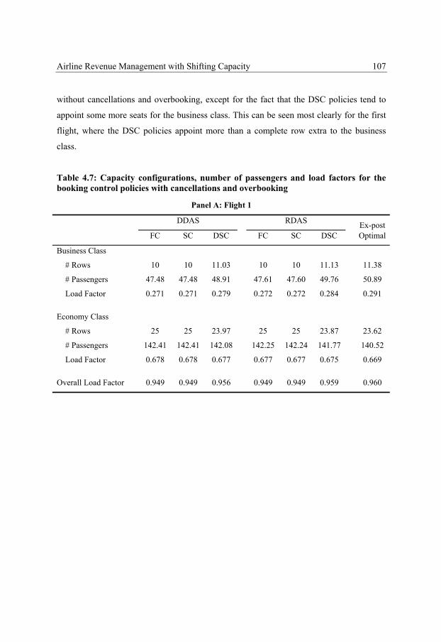
117
Airline Revenue Management with Shifting Capacity 107
without cancellations and overbooking, except for the fact that the DSC policies tend to
appoint some more seats for the business class. This can be seen most clearly for the first
flight, where the DSC policies appoint more than a complete row extra to the business
class.
Table 4.7: Capacity configurations, number of passengers and load factors for the booking control policies with cancellations and overbooking
Panel A: Flight 1
DDAS RDAS Ex-post FC SC DSC FC SC DSC Optimal
Business Class
# Rows 10 10 11.03 10 10 11.13 11.38
# Passengers 47.48 47.48 48.91 47.61 47.60 49.76 50.89
Load Factor 0.271 0.271 0.279 0.272 0.272 0.284 0.291
Economy Class
# Rows 25 25 23.97 25 25 23.87 23.62
# Passengers 142.41 142.41 142.08 142.25 142.24 141.77 140.52
Load Factor 0.678 0.678 0.677 0.677 0.677 0.675 0.669
Overall Load Factor 0.949 0.949 0.956 0.949 0.949 0.959 0.960
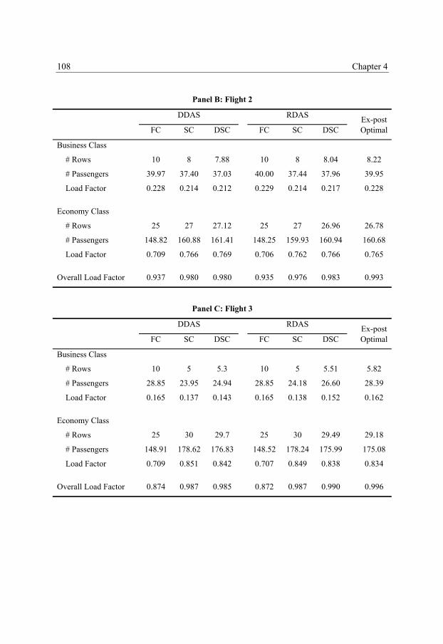
118
Chapter 4 108
Panel B: Flight 2
DDAS RDAS Ex-post FC SC DSC FC SC DSC Optimal
Business Class
# Rows 10 8 7.88 10 8 8.04 8.22
# Passengers 39.97 37.40 37.03 40.00 37.44 37.96 39.95
Load Factor 0.228 0.214 0.212 0.229 0.214 0.217 0.228
Economy Class
# Rows 25 27 27.12 25 27 26.96 26.78
# Passengers 148.82 160.88 161.41 148.25 159.93 160.94 160.68
Load Factor 0.709 0.766 0.769 0.706 0.762 0.766 0.765
Overall Load Factor 0.937 0.980 0.980 0.935 0.976 0.983 0.993
Panel C: Flight 3
DDAS RDAS Ex-post FC SC DSC FC SC DSC Optimal
Business Class
# Rows 10 5 5.3 10 5 5.51 5.82
# Passengers 28.85 23.95 24.94 28.85 24.18 26.60 28.39
Load Factor 0.165 0.137 0.143 0.165 0.138 0.152 0.162
Economy Class
# Rows 25 30 29.7 25 30 29.49 29.18
# Passengers 148.91 178.62 176.83 148.52 178.24 175.99 175.08
Load Factor 0.709 0.851 0.842 0.707 0.849 0.838 0.834
Overall Load Factor 0.874 0.987 0.985 0.872 0.987 0.990 0.996
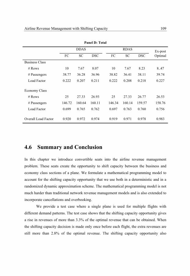
119
Airline Revenue Management with Shifting Capacity 109
Panel D: Total
DDAS RDAS Ex-post FC SC DSC FC SC DSC Optimal
Business Class
# Rows 10 7.67 8.07 10 7.67 8.23 8..47
# Passengers 38.77 36.28 36.96 38.82 36.41 38.11 39.74
Load Factor 0.222 0.207 0.211 0.222 0.208 0.218 0.227
Economy Class
# Rows 25 27.33 26.93 25 27.33 26.77 26.53
# Passengers 146.72 160.64 160.11 146.34 160.14 159.57 158.76
Load Factor 0.699 0.765 0.762 0.697 0.763 0.760 0.756
Overall Load Factor 0.920 0.972 0.974 0.919 0.971 0.978 0.983
4.6 Summary and Conclusion
In this chapter we introduce convertible seats into the airline revenue management
problem. These seats create the opportunity to shift capacity between the business and
economy class sections of a plane. We formulate a mathematical programming model to
account for the shifting capacity opportunity that we use both in a deterministic and in a
randomized dynamic approximation scheme. The mathematical programming model is not
much harder than traditional network revenue management models and is also extended to
incorporate cancellations and overbooking.
We provide a test case where a single plane is used for multiple flights with
different demand patterns. The test case shows that the shifting capacity opportunity gives
a rise in revenues of more than 3.3% of the optimal revenue that can be obtained. When
the shifting capacity decision is made only once before each flight, the extra revenues are
still more than 2.8% of the optimal revenue. The shifting capacity opportunity also
120
Chapter 4 110
increases the load factor of the plane from 92% to more than 97%. When cancellations and
overbooking are taken into account these results remain the same. We also observe that
taking the shifting capacity opportunity into account can result in a policy that is less
careful with respect to overbooking. This is because the opportunity costs of a booking
can become very large whenever the booking is blocking an entire row from becoming
available for the other section of the plane. Therefore, it can be worthwhile in some cases
to take the risk of a denied boarding. Further, we see that randomization of the booking
control policy in order to account for the stochastic nature of demand, increases the
performance of the policies, but never more than 0.7% of the optimal revenue that can be
obtained. The computation time of such a randomized policy is however considerably
larger then for a deterministic policy.
This study provides a way to model the shifting capacity decision and gives an
indication of the added value of doing so. The booking control policies that we used are
computationally very cumbersome and will not always be applicable in practice in this
exact way. Therefore, a study on computationally less demanding booking control policies
could prove useful. For this, one can think of bid prices that serve as approximations of
the opportunity costs for a longer period of time or nested booking limits that determine
the number of booking requests to accept for each price class. Both can be based on the
models introduced in this study. Further, we acknowledge that our test case is but an initial
one and many more can be constructed to obtain further insights. For example, our test
case consists of a single flight, which gives us the opportunity to illustrate things more
clearly, and does not include multiple seat booking requests. Finally, we would like to
mention that most extensions to the standard airline network revenue management
problem that are suggested throughout the literature can be applied to the model that we
provide in this study as well. This comes forth from the fact that our model still resembles
the standard revenue management models very much.
121
Chapter 5 Cargo Revenue Management: Bid Prices for a 0-1 Multi Knapsack Problem
5.1 Introduction
Revenue management gained popularity in the airline industry where passengers that
compete for the same seat in a plane generally pay different prices. The principles of
revenue management can also be applied to cargo transportation. Although this is already
done in practice, little research can be found on cargo revenue management. The solution
techniques used for the cargo revenue management problem are therefore basically the
same as the techniques constructed for the well-known passenger revenue management
problem. However, cargo revenue management differs from the passenger revenue
management problem in a number of ways. Particularly, by the fact that its capacity
constraint is 2-dimensional, i.e. weight and volume, and that the weight, volume and profit
of each booking request are random and continuous variables. Passenger revenue
management solution techniques are generally based on the fact that the booking requests
can be categorized in different price classes. Cargo shipments, however, are not defined
122
Chapter 5 112
over such price classes but are uniquely defined by their profit, weight and volume.
Without this kind of categorization into distinct classes, the question is whether a revenue
management policy can be constructed for the unique cargo booking requests which is still
simple and effective for practical use.
In this chapter, we present such a booking control policy. The booking requests are
considered to be unique items, which means that we consider a 0-1 decision problem.
Since a cargo shipment can use multiple connecting flights to reach its destination and the
accept/deny decision has to be made as the booking request occurs, we model the problem
as a 0-1 multi-dimensional on-line knapsack problem. We show that a bid-price
acceptance policy is asymptotically optimal if demand and capacity increase
proportionally and the bid prices are set correctly. Further, we present a heuristic to obtain
values for the bid prices based on a greedy algorithm for the 0-1 multi-dimensional
knapsack problem proposed by Rinnooy Kan et al. (1993). The performance of the
knapsack bid prices is evaluated together with other booking control policies in a
simulated environment.
In Section 5.2 we discuss the cargo revenue management problem and its
differences with the airline passenger revenue management problem. We provide a
mathematical formulation of the problem in Section 5.3. In this section we discuss the
optimal control policy, a dynamic approximation scheme for it and the bid-price policy. In
Section 5.4 we present a polynomial time algorithm to obtain values for the bid-price
policy. In Section 5.5 we discuss the test case that we construct and report the
performance of the various booking control policies. Finally, we conclude this chapter in
Section 5.6.
5.2 Cargo Revenue Management
The revenue management applications that we discussed in the previous chapters are
aimed at accepting those customers that maximize the revenue for the company. Because
the capacity is generally fixed and has to be sold before a deadline, there is a trade off
123
Cargo Revenue Management: Bid Prices for a 0-1 Multi Knapsack Problem 113
between accepting a booking request with a certain revenue and waiting for a more
profitable booking request that may or may not come. It is well known that the principles
of revenue management can also be applied to cargo transportation (see: Kasilingam
(1996)). Although a large part of the cargo capacity is usually consumed by shipments that
are determined by long-term contracts, also a certain part of the capacity is generally kept
available for on-the-spot sales that tend to be more profitable per kg. Booking requests for
these spot sales come in during the booking period and have to be accepted or rejected as
they come in. The allocation of the cargo capacity over the long-term contracts and the
spot sales is an interesting research topic on itself, but we will not go into this problem in
this study. The problem that we consider is that of accepting or rejecting the spot sales as
they come in during the booking period.
In Section 5.2.1 we discuss the differences between the cargo and passenger
revenue management problems and in Section 5.2.2 we discuss the related literature on
cargo revenue management.
5.2.1 Cargo vs. Passenger Revenue Management
Cargo revenue management differs from passenger revenue management in a number of
ways. The most important difference is that two passengers who book in the same price
class for a flight can be seen as two identical customers, whereas each cargo shipment is
unique. The two passengers both take up one seat, have the same ticket options, generate
the same revenue, etc. This generally results in revenue management policies that
determine how many passengers to accept in each price class, or whether or not a specific
price class is open for booking at a certain time. Also for cargo transportation there are
usually a number of different product types, e.g. mail, fresh products, live animals,
secured products and door-to-door service. However, the profit generated by a shipment
does not just depend on the price, but also on the additional costs associated to the
shipment, e.g. special packaging, additional trucking and fuel. In addition, cargo booking
requests are generally made by a limited number of large customers. These customers
124
Chapter 5 114
have more purchasing power than a potential passenger for a flight. It is no exception that
the price for a potential cargo shipment is subject to negotiation before the actual booking
request is made. These things combined, mean that next to the weight and volume, also
the profit per kg of a cargo shipment is a random variable. The profit, weight and volume
all take on continuous values and differ for all shipments. The uncertainty in passenger
revenue management lies in the number of passengers that will arrive for each price class,
whereas for cargo revenue management each shipment is a unique item with properties
that are not known before the time of booking.
Unlike passenger capacity, the cargo capacity available for the spot sales is
generally uncertain. This capacity does not only depend on the capacity taken up by the
long-term contracts, but also on the weather conditions, the amount of fuel needed for the
trip and more. For a combi-plane, which is used to carry both passengers and cargo, also
the number of passengers and the weight and volume of their luggage have to be
considered. Further, the actual amount of cargo usually deviates from the initial booking
request, especially for the long-term contracts. This means that overbooking is an
important aspect of cargo revenue management. In this study, however, we assume that
the cargo capacity available for the spot sales is known. This is in line with other revenue
management studies, where uncertainties about the capacity and overbooking are usually
left out in order to focus on the booking control policy. We notice, however, that common
overbooking techniques can be used in combination with the policies that we present in
this study.
Passenger revenue management is usually looked at from a network perspective.
That is, a passenger that uses multiple connected flights, should be evaluated according to
its overall profit to the flight network and not for each flight individually. This is also the
case for cargo shipments and the model that we provide takes this into account.

125
Cargo Revenue Management: Bid Prices for a 0-1 Multi Knapsack Problem 115
5.2.2 Literature
Although cargo transportation is generally recognized as a natural application for revenue
management, it has not received a lot of attention in the literature. In fact, Kasilingam
(1996) and Karaesmen (2001) are the only studies that we know that concentrate on cargo
revenue management. Kasilingam (1996) concentrates on air cargo and discusses the
differences between passenger and cargo revenue management for an airline company.
Besides the differences discussed in the previous section, he points out that cargo has the
possibility to be shipped among different routes as long as it gets to its destination in time.
He also indicates that the number of positions when working with containers is limited.
This can be another capacity restriction. Our experience with KLM Royal Dutch Airlines,
however, tells us that positioning is hardly a problem for air cargo, since the airline
company generally builds pallets itself instead of using containers. The revenue
management model that Kasilingam describes is very similar to the standard mathematical
programming models known from passenger revenue management. We do not think this
kind of model suits the cargo problem since cargo shipments can not be classified into
groups (price classes) with identical properties as passengers can.
Karaesmen (2001) formulates the cargo revenue management problem as a
continuous linear programming problem and shows that optimal bid prices exist for the
problem. In order to obtain bid-price values, she discretizes the state space into weight and
volume regions. Such a discretization corresponds with grouping the cargo shipments into
a limited number of classes with identical properties. The model proposed by Kasilingham
(1996) can then be used to obtain the bid prices. How to group the cargo shipments into
distinct classes is not trivial. In this study, we propose a model that does not group the
cargo shipments, but instead treats them as the unique items that they are. This leads us to
a 0-1 multi-dimensional on-line knapsack problem.
In a series of articles, Kleywegt and Papastavrou investigate what they call the
dynamic stochastic knapsack problem (see: Papastavrou et al. (1996), Kleywegt and
Papastavrou (1998) and Kleywegt and Papastavrou (2001)). They mention its application
to cargo revenue management. However, their models include only one capacity

126
Chapter 5 116
restriction. They choose a dynamic programming approach to the problem which,
although theoretically very interesting, is computationally very demanding. Especially
when a second capacity restriction is added to this approach, the state space will become
intractable for practical use. Our approach is a static but more efficient and practical one.
The bid-price solution technique that we use in this study, has been discussed
extensively by Talluri and van Ryzin (1998) for the passenger revenue management
problem. They show that bid prices are not optimal in general, but are asymptotically
optimal when capacity and demand increase proportionally. Their model differs from ours
in the sense that they divide the booking requests into classes in such a way that two
requests in the same class always have the same capacity requirement. This is not the case
in our problem where every shipment has a random weight and volume. Nevertheless, we
show that the asymptotic optimality holds in our case as well.
5.3 Problem Formulation
The cargo revenue management problem as we define it in this study is such that a number
of booking requests come in during the booking period. Each booking request is uniquely
defined by its weight, volume, profit and the flights it uses. The number of shipments that
the airline company can accept on a flight is determined by the weight and volume
capacities of the plane. We assume that the capacities are fixed and given and that the
actual weight and volume of the shipments do not differ from the booked quantities. We
do not consider cancellations and overbooking. Finally, as common in quantity-based
revenue management, we assume that demand is independent of the booking control
policy used.
In Section 5.3.1 we formulate the theoretical optimal control policy for the
problem. A dynamic approximation scheme and the bid-price policy are discussed in
Section 5.3.2 and Section 5.3.3 respectively.

127
Cargo Revenue Management: Bid Prices for a 0-1 Multi Knapsack Problem 117
5.3.1 Optimal Control
The decision to accept or reject a booking request has to be made at the moment the
request comes in. This decision depends on the remaining capacities, the expected future
demand and the properties of the booking request. We model the booking requests as a
sequence of arrivals over time and measure time in discrete intervals counting backwards,
i.e. at time 0 the process ends. We assume each time interval to be small enough such that
no more than one request will occur within a time interval. Because a shipment can use
more than one flight to reach its destination, we include multiple flights in our model.
Assume there are m flights that have weight and volume capacities given by the vectors cw
= (cw,1, cw,2, ..., cw,m)T and cv = (cv,1, cv,2, ..., cv,m)T. The capacities cannot be negative and
are adjusted every time a booking request is accepted. Define ),( vwtJ cc as the optimal
expected revenue that can be generated with t time units to go and capacities cw and cv
available. We know that ),( vwtJ cc must satisfy:
0),( ≥vwtJ cc ∀ cw, cv, t
0),(0 =vwJ cc ∀ cw, cv
0)0,(),0( == wtvt JJ cc ∀ cw, cv, t.
Further, we know that ),( vwtJ cc is non-decreasing in t, cw and cv, since it is never a
disadvantage to have more time or capacity available. For a more exhaustive analysis of
the expected reward function, we refer to Papastavrou et al. (1996), who discuss various
special cases of the problem.
In order to formulate the Bellman equation for the problem, define Rt as the
random variable that denotes the profit of a booking request that is made with t time
periods to go. Note that Rt = 0 when no booking request occurs. Also define the random
vectors Wt = (Wt,1, Wt,2, …, Wt,m)T and Vt = (Vt,1, Vt,2, …, Vt,m)T that give the weight and
volume requirements of the booking request on the m flights. This means that if a booking
request is made with t time periods to go, Wt,i is equal to the weight of the shipment if the

128
Chapter 5 118
shipment uses flight i (i = 1, 2, ..., m) and 0 for all other flights. This is the same for Vt,i.
Further, let x be the control variable denoting whether to accept a booking request (x = 1)
or not (x = 0). Then, x is restricted to the set vtwtvwt cxxxX ≤≤∈= VcWcc ,:1,0),(
and the Bellman equation is given by:
⎥⎦⎤
⎢⎣⎡ −−+= −∈
),(max),( 1),( vvtwttXvwt xcxJxREJvwt
VWcccccx
, (5.1)
with the boundary conditions provided above.
Whenever a booking request comes in with t time units to go and capacities cw and
cv available, its profit and its weight and volume requirements are observed. We denote
the observed profit by r and the observed weight and volume requirements by w = (w1, w2,
…, wm)T and v = (v1, v2, …, vm)T. The optimal control policy provided by (5.1) says to
accept the booking request if and only if sufficient capacity is available and:
),(),( 11 vcwccc −−−≥ −− vwtvwt JJr . (5.2)
The left hand side of (5.2) denotes the direct revenue associated with accepting the cargo
shipment, whereas the right hand side gives the estimated opportunity costs of the
capacities taken up by the shipment.
The optimal control policy is similar to the one known for passenger revenue
management presented in Chapter 2. Except that in the passenger case, there is only one
capacity dimension and the size of a demand is restricted to a limited number of integer
values (and generally even considered to be equal to one). Lautenbacher and Stidham
(1999), Lee and Hersh (1993), Liang (1999) and Subramanian et al. (1999), use a dynamic
programming approach to the passenger problem for a single flight. Van Slyke and Young
(2000) also consider multiple flights, but acknowledge that the complexity introduced by
the increased number of dimensions is tremendous. For the cargo problem, which has two
capacity dimensions and continuous demand sizes, a dynamic programming approach
becomes computationally intractable. In the next section we discuss a dynamic

129
Cargo Revenue Management: Bid Prices for a 0-1 Multi Knapsack Problem 119
approximation scheme for the problem and in Section 5.3.3 we construct a bid-price
policy that is well suited for use in practice.
5.3.2 Dynamic Approximation Scheme
In this section we construct a dynamic approximation scheme that can be used for the on-
line accept/deny decision. We propose a method to approximate the optimal expected
revenue that can be generated for a given set of capacities and a given time to go, i.e.
),( vwtJ cc . This way, approximations for ),( vwtJ cc and ),( vcwc −− vwtJ can be
computed whenever a booking request comes in. These approximations can then be used
to apply the control policy provided by (5.2).
If the future demand is known, we can easily compute the optimal future revenue
by formulating the problem as a deterministic mathematical programming problem.
Assume that we have a given set of n booking requests that define the problem instance Ω.
Let the profits of the booking requests be given by the vector r = (r1, r2, ..., rn)T. Further,
define the matrix Aw = [aw,ij], such that aw,ij is equal to the weight of shipment j if that
shipment uses flight i and 0 otherwise. Likewise, define the matrix Av for the volume
requirements of the shipments. Let ),( vwtJ ccΩ be the optimal future revenue that can be
generated for problem instance Ω with t time units to go and capacities cw and cv available,
then ),( vwtJ ccΩ can be obtained from the following integer programming problem:
=Ω ),( vwtJ cc max xr T (5.3)
s.t. ww cxA ≤
vv cxA ≤
n1,0∈x ,
130
Chapter 5 120
where x = (x1, x2, ..., xn)T determines whether booking request j is accepted (xj = 1) or not
(xj = 0). This model is known to be NP-hard (see Garey and Johnson (1979)). Standard
integer programming solution methods, such as branch-and-bound, can be used to solve
small problem instances of the model. For bigger problem instances Rinnooy Kan et al.
(1993) provide a polynomial time greedy algorithm that provides an asymptotically
optimal solution when demand and capacity increase proportionally. We discuss this
algorithm in detail in the Section 5.4.
In practice, the future demand is not known. In passenger revenue management it
is common practice to formulate a mathematical programming model for the expected
demands for the various route/price-class combinations in order to obtain an
approximation of the optimal future revenue. However, this is not an option for the cargo
revenue management problem since cargo shipments cannot be categorized into distinct
classes. Therefore, we suggest to compute the optimal future revenue for a series of
simulated demand instances, i.e. ),(1vwtJ ccΩ , ),(2
vwtJ ccΩ , ..., ),( vwtkJ ccΩ . An
approximation for ),( vwtJ cc can then be obtained by taking the average value over the
simulated instances. Doing this every time a booking request comes in, is not as
intractable as dynamic programming. However, it still is computationally very demanding.
In the next section, we construct a bid-price policy that does not require any on-line
computation time and is therefore easy to use in practice.
5.3.3 Bid Prices
Bid-price acceptance policies are widely used in passenger revenue management. The idea
of a bid-price policy is to determine a value for which a unit of capacity can be sold at a
certain point in time. This way, the opportunity costs of a booking request can be
approximated by the sum of the bid prices of the capacities it uses. The booking request is
only accepted if its profit exceeds the opportunity costs. A bid price is determined for
every dimension of the capacity, which in our case would mean one weight and one
volume bid price for each flight. Optimally, the bid price is a function of the remaining
131
Cargo Revenue Management: Bid Prices for a 0-1 Multi Knapsack Problem 121
time and capacity. In practice, however, the function is usually approximated by a fixed
value that is re-evaluated at fixed points in time.
When the bid prices for the different capacity dimensions are held constant for a
longer period of time, the approximation of the opportunity costs of a booking request
reduces to a linear combination of the capacity requirements of the request. In order to see
this, let µw = (µw,1, µw,2, ..., µw,m)T and µv = (µv,1, µv,2, ..., µv,m)T be the bid prices for the
weight and volume capacities of the flights. Then, if a booking request comes in with
profit r, and capacity requirements w and v, it is accepted under the bid-price policy if and
only if sufficient capacity is available and:
vµwµ TTvwr +≥ , (5.4)
which is the sum of the bid prices of the capacities it uses multiplied by the sizes of the
capacity requirements. Bid prices are studied extensively for passenger revenue
management by Talluri and van Ryzin (1998). They show that when the bid prices are set
correctly, a static bid-price policy is asymptotically optimal when the capacities and the
demand increase proportionally. We show that this also holds for the cargo problem.
In a probabilistic error analysis, Rinnooy Kan et al. (1993) show that a static bid-
price policy is asymptotically optimal for the 0-1 multi-dimensional knapsack problem.
They consider a probabilistic version of model (5.3) by letting the profit and the weight
and volume requirements of the items in the knapsack be independent identically
distributed random variables. Assume that the capacities grow proportionally with the
number of items, i.e. cw,i = nβw,i and cv,i = nβv,i, where βw,i and βv,i are fixed values (i = 1,
2, …, m). Finally, define zn as the random variable that denotes the optimum solution
value of the problem with n items and ),( vwnz µµ as the random variable that denotes the
solution value when the items are accepted by the bid-price policy that uses the bid prices
µw and µv. Then under certain conditions concerning the probability distributions, Rinnooy
Kan et al. (1993) show that the sequence /),( nvwn zz µµ converges to 1 with probability
one if µw and µv are chosen correctly. For an intuitive clarification, note that it is the
132
Chapter 5 122
combinatorial aspect of the problem that creates a gap between the optimal and the greedy
solutions. In fact, if all items were of the same size, the greedy algorithm would provide
the optimal solution. Now, by increasing the number of items and the capacity along with
it, the size of each individual item becomes less influential and so does the combinatorial
aspect of the problem. Eventually, as the number of items goes to infinity, the
combinatorial effect dies out.
We argue that the on-line decision problem that we study in this study, can be
formulated in the exact same way as discussed above, which means that the asymptotic
result holds for our problem as well. As portrait in Section 5.3.1, we can assume that there
is a booking request for every decision period without loss of generality. This holds,
because we can always consider a booking request to have a profit, weight and volume of
value 0. We can now interpret the on-line problem as a 0-1 decision problem for every
decision period. When we formulate this as a knapsack problem we let the decision
variables in the knapsack correspond to the decision periods in the booking process. This
way, all random elements of the problem are modelled in the profit and capacity
requirement coefficients, which gives us the model studied by Rinnooy Kan et al. (1993).
Thus, also for the cargo revenue management problem, a bid-price policy is
asymptotically optimal as demand and capacity increase proportionally and the bid prices
are chosen correctly.
5.4 Obtaining Bid Prices
In passenger revenue management, bid prices are often approximated by the dual prices of
the LP-relaxation of the underlying mathematical programming model which determines
the allocation of the capacity over the demand. The cargo problem, however, is a 0-1
decision problem for which the LP-relaxation is a very crude approximation. In this
section we provide polynomial time algorithm to obtain optimal bid prices for a given set
of booking requests based on a greedy algorithm for the 0-1 multi-dimensional knapsack

133
Cargo Revenue Management: Bid Prices for a 0-1 Multi Knapsack Problem 123
problem. In Section 5.4.1 we give the general idea of the greedy algorithm. In Section
5.4.2 we discuss how to obtain bid prices and the computational complexity of doing so.
5.4.1 Greedy Algorithm
In order to obtain bid prices, we make use of a greedy algorithm that Rinnooy Kan et al.
(1993) present for the 0-1 multi-dimensional knapsack problem. The idea of the greedy
algorithm is to weigh each capacity dimension and select those items in the knapsack that
have the highest profit per weighted capacity requirement. Assume that αw = (αw,1, αw,2,
..., αw,m)T and αv = (αv,1, αv,2, ..., αv,m)T are the non-negative weights for the weight and
volume capacities on the flights. As before, let r, w and v be the profit and the weight and
volume requirements of a booking request. Then the booking requests that are accepted,
are those that have the highest ratio:
vαwα TTvw
r+
=δ (5.5)
In order to understand how the greedy algorithm works, notice that from (5.5) we
know that we want to select those booking requests for which the values w/r and v/r are
small. That is, those requests that do not use a lot of capacity for the profit they provide.
For a graphical representation, let each booking request correspond to a point in m2+ℜ ,
given by the coordinates (w1/r, w2/r, ..., wm/r, v1/r, v2/r, ..., vm/r). Then, the greedy
algorithm can be regarded as a hyperplane with normal vector (αw,1, αw,2, ..., αw,m, αv,1,
αv,2, ..., αv,m) that moves upward from the origin and accepts booking request in the order
that it encounters them. This is depicted for a single flight in Figure 5.1. For this 2-
dimensional case, the hyperplane is reduced to a line with the slope αw/αv.

134
Chapter 5 124
Figure 5.1: Accepting booking requests for a single flight with the greedy algorithm.
For a given set of booking requests, one can simply select those requests that have
the highest δ. For the on-line problem, however, the future booking requests are not
known. Therefore, a threshold value for δ has to be specified in advance. If δ is the
threshold value, then a booking request with profit r and capacity requirements w and v is
accepted if and only if sufficient capacity is available and:
δTT ≥+ vαwα vw
r , (5.6)
which is the same as:
)(ˆ TT vαwα vwr +≥ δ . (5.7)
This means that the greedy algorithm can be seen as a bid-price policy, where the bid
prices are set equal to wαδ and vαδ . In terms of Figure 5.1, αw and αv define the slope of
the line and the threshold value δ determines the height of the line.
w/r
v/r
135
Cargo Revenue Management: Bid Prices for a 0-1 Multi Knapsack Problem 125
5.4.2 Computational Complexity of Finding Bid Prices
The greedy algorithm presented in the previous section gives another interpretation to the
well-known bid prices. The bid prices are defined by a set of weights with a corresponding
threshold value. For a given set of booking requests, Rinnooy Kan et al. (1993) provide a
polynomial time algorithm to determine optimal values for the weights and the threshold
value when the number of capacity dimensions is not more than the number of booking
requests. They show that the problem becomes NP-hard if the number of capacity
dimensions exceeds the number of requests. Since there are only two capacity dimensions
in the cargo revenue management problem, this is already ruled out as soon as there are
two booking requests per flight. Notice that for a given set of booking requests, each set of
weights brings forth an ordering in which the requests are considered for acceptance.
However, we need only consider those sets of weights that actually induce a different
ordering. That is, we only need to consider those sets of weights that construct a
sufficiently different hyperplane such that it encounters the booking requests in a different
order as it moves up from the origin. In the case of one flight, and thus 2-dimensions, with
n booking requests, there are at most ⎟⎟⎠
⎞⎜⎜⎝
⎛2n
of such changes in the ordering.
Lenstra et al. (1982) provide an algorithm that can be used to determine all
possible orderings. In terms of Figure 5.1, the algorithm makes use of the fact that the line
that passes through two booking requests, provides exactly that slope for which the
requests are swapping places in the ordering. Thus, in order to obtain all orderings, we
only have to determine those lines that connect two booking requests. Note that we only
have to consider negative slopes, since a positive slope does not provide an ordering of the
requests. Let xj = (w/r)j and yj = (v/r)j denote the weight and volume per profit for booking
request j (j = 1, 2, ..., n). Lenstra et al. (1982) suggest to first order the requests by the
sequence njjx 1 = and then to determine the line that passes through requests k and l for all
k = 1, 2, ..., n and l = 1, 2, ..., n for which k < l (i.e. lk xx ≤ ) and lk yy ≥ . For each

136
Chapter 5 126
ordering that can be obtained, one can simply compute the solution of the greedy
algorithm by accepting the requests until the capacity is full.
Determining the orderings by the algorithm provided by Lenstra et al. (1982) can
be done in O(n2 log n) time. Filling the capacity for a specific ordering costs at most O(n)
time. Finally, selecting the ordering that produces the highest profit costs O(log n) time.
This means that the total computation time is O(n3 log n). When we consider m flights, the
total number of exchanges is O(n2m). They can be determined in O(n2m log n) time, such
that the total computation time is O(n2m+1 log n). This is polynomial in n for a given
number of flights m. For the case of one flight, a schematic overview of the algorithm is
given in Figure 5.2. This can easily be extended to the case of m flights.
Figure 5.2: Schematic overview of the algorithm for obtaining optimal bid prices.
Given: A number of n booking requests defined by njjj yx 1),( = , where xj and yj are
the weight and volume per profit for booking request j.
Step 1: Order the requests by increasing value of xj.
Step 2: For k = 1 to n:
For l = k+1 to n and lk yy ≥ :
Let kl
kl
xxyy
−−
=γ .
For h = 1 to n: let ηh = yh - γxh.
Order the requests by increasing value of ηh.
Start accepting requests in this order until no more requests can be accepted.
Let π be the profit obtained and let η be the order value for the last request
that is accepted.
Step 3: Find the maximum profit π* over all orderings.
Let γ* and η* be the corresponding slope and order value.
Return: µw = -γ*/η* and µv = 1/η*.
137
Cargo Revenue Management: Bid Prices for a 0-1 Multi Knapsack Problem 127
The algorithm discussed above, provides a way to obtain the optimal bid prices for
a given set of booking requests. In practice, the bid prices have to be set before the
demand is known. An easy way to obtain bid prices is to simulate a series of demand
sequences, compute the optimal bid prices for each sequence and set the bid prices that are
used for the on-line policy to the average values over all sequences.
5.5 Test Case
In this section we present computational results for the solution methods described in the
previous sections when they are applied to a simulated test case. The test case that we
consider is a realistic one that reflects the situation that we encountered in practice at
KLM Royal Dutch Airlines. We obtain results for the bid-price policy when the bid prices
are determined by: (i) the algorithm for the 0-1 multi-dimensional knapsack problem and
(ii) the dual prices of the LP-relaxation of the problem. We compare the performance of
the bid-price policies to that of the dynamic approximation scheme and the ex-post
optimal solution that can be obtained with hindsight when all demand is known.
In Section 5.5.1 we first describe the test case that we construct. In Section 5.5.2
we present the computational results which we extend in Section 5.5.3 for different
capacity/demand ratios.
5.5.1 Description of the Test Case
The test case that we construct consists of a single flight with a fixed weight and volume
capacity of 10000 kg and 75 m3 respectively. These are the capacities available for the
spot sales after correcting the total capacity of the plane for the space taken up by the
long-term cargo contracts. The booking period is made up of T discrete time intervals of
length one. Booking requests come in according to a Poisson arrival process with an
arrival rate λ. This means that with probability λ a booking request is made in a time

138
Chapter 5 128
period and with probability 1-λ there is not. The total expected number of booking
requests is therefore λT and the maximum number of requests is T.
Each booking request has a unique profit, weight and volume that we denote by r,
w and v respectively. The profit, weight and volume are related to each other since they all
reflect the size of the shipment. To get around this problem, we define the profit and
volume relative to the weight of the shipment and assume the variables w, r/w and v/w to
be independent random variables. We assume all booking requests to be independent
identically distributed and consider w, r/w and v/w to follow a log-normal distribution. The
log-normal distribution generates values that resemble the data that we encountered in
practice. We note, however, that we do not try to model the large amount of very small
shipments, of for example 1, 2, 10 or 20 kg that an airline company usually has to deal
with. These small shipments are generally highly profitable per kg and take up very little
capacity. This means that they are almost always accepted and in practice are often not
even subjected to the revenue management decision rule. More than anything, these
shipments are used to fill up the wholes in the capacity that are left by the bigger
shipments. We choose to exclude the small shipments from the test case such that the
algorithm that sets the bid prices is not influenced by these relatively insignificant
shipments. Moreover, note also that it does not seem worthwhile to accurately model
shipments of 2 kg next to shipments of 1000 kg. A small error in the latter can easily be
greater than the first shipment as a whole.
The parameters of the simulation are given in Table 5.1, whereas a graphical
presentation of the probability density functions of w, r/w and v/w up until the 99th
percentile are given in Figure 5.3. We note that the capacities and the demand are chosen
to reflect a real life situation and correspond to capacity/demand ratios of 0.56 and 0.72
for the weight and volume respectively. However, in Section 5.5.3 we present
computational results for various levels of the capacity/demand ratios. Finally, we mention
that we do not consider cancellations, no-shows or deviations from the requested capacity
requirements. Neither do we allow overbooking.
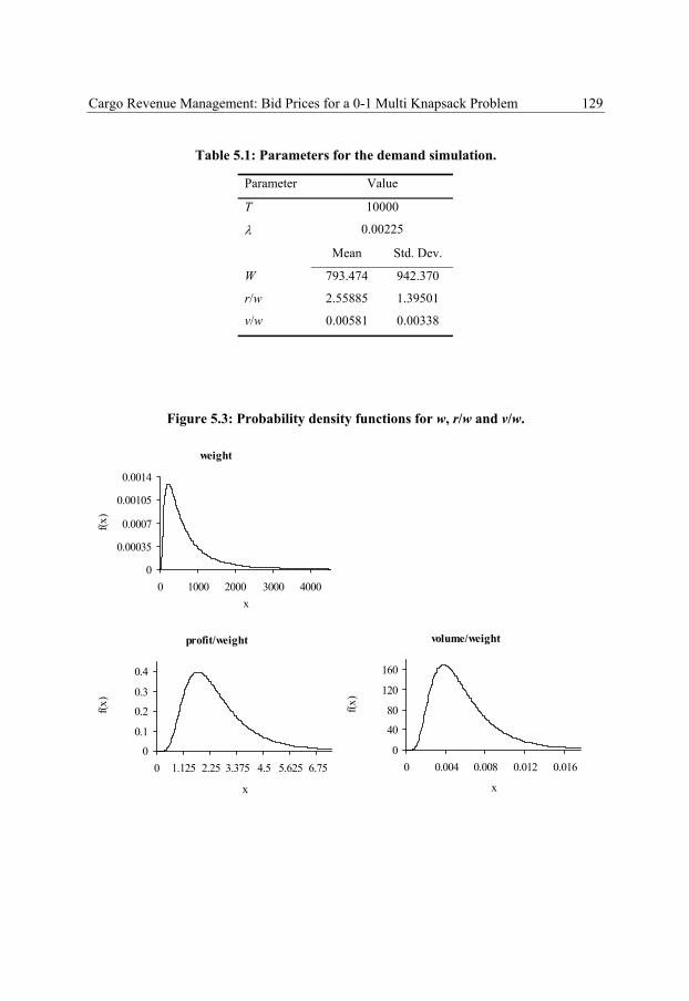
139
Cargo Revenue Management: Bid Prices for a 0-1 Multi Knapsack Problem 129
Table 5.1: Parameters for the demand simulation.
Parameter Value
T 10000
λ 0.00225
Mean Std. Dev.
W 793.474 942.370
r/w 2.55885 1.39501
v/w 0.00581 0.00338
Figure 5.3: Probability density functions for w, r/w and v/w.
weight
0
0.00035
0.0007
0.00105
0.0014
0 1000 2000 3000 4000x
f(x)
profit/weight
0
0.1
0.2
0.3
0.4
0 1.125 2.25 3.375 4.5 5.625 6.75
x
f(x)
volume/weight
0
40
80
120
160
0 0.004 0.008 0.012 0.016
x
f(x)
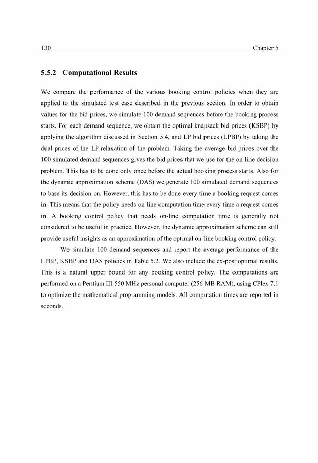
140
Chapter 5 130
5.5.2 Computational Results
We compare the performance of the various booking control policies when they are
applied to the simulated test case described in the previous section. In order to obtain
values for the bid prices, we simulate 100 demand sequences before the booking process
starts. For each demand sequence, we obtain the optimal knapsack bid prices (KSBP) by
applying the algorithm discussed in Section 5.4, and LP bid prices (LPBP) by taking the
dual prices of the LP-relaxation of the problem. Taking the average bid prices over the
100 simulated demand sequences gives the bid prices that we use for the on-line decision
problem. This has to be done only once before the actual booking process starts. Also for
the dynamic approximation scheme (DAS) we generate 100 simulated demand sequences
to base its decision on. However, this has to be done every time a booking request comes
in. This means that the policy needs on-line computation time every time a request comes
in. A booking control policy that needs on-line computation time is generally not
considered to be useful in practice. However, the dynamic approximation scheme can still
provide useful insights as an approximation of the optimal on-line booking control policy.
We simulate 100 demand sequences and report the average performance of the
LPBP, KSBP and DAS policies in Table 5.2. We also include the ex-post optimal results.
This is a natural upper bound for any booking control policy. The computations are
performed on a Pentium III 550 MHz personal computer (256 MB RAM), using CPlex 7.1
to optimize the mathematical programming models. All computation times are reported in
seconds.
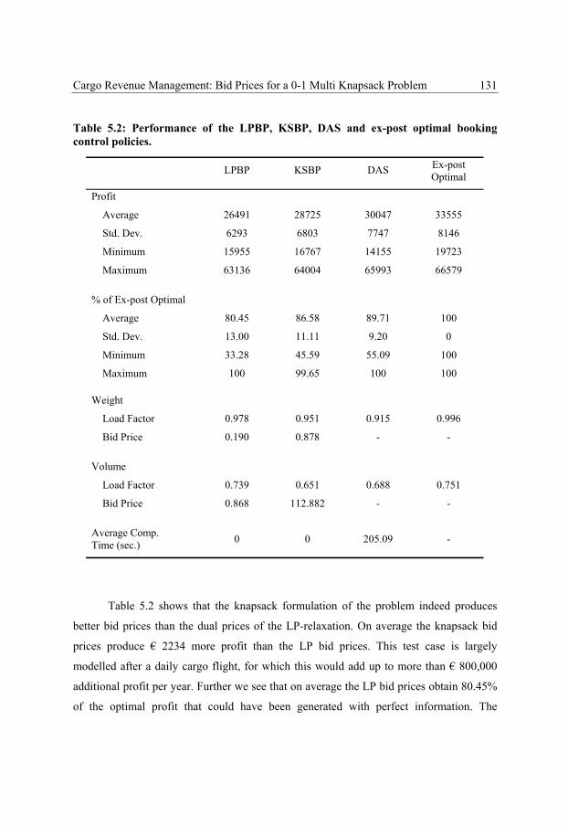
141
Cargo Revenue Management: Bid Prices for a 0-1 Multi Knapsack Problem 131
Table 5.2: Performance of the LPBP, KSBP, DAS and ex-post optimal booking control policies.
Ex-post LPBP KSBP DAS Optimal
Profit
Average 26491 28725 30047 33555
Std. Dev. 6293 6803 7747 8146
Minimum 15955 16767 14155 19723
Maximum 63136 64004 65993 66579
% of Ex-post Optimal
Average 80.45 86.58 89.71 100
Std. Dev. 13.00 11.11 9.20 0
Minimum 33.28 45.59 55.09 100
Maximum 100 99.65 100 100
Weight
Load Factor 0.978 0.951 0.915 0.996
Bid Price 0.190 0.878 - -
Volume
Load Factor 0.739 0.651 0.688 0.751
Bid Price 0.868 112.882 - -
Average Comp. Time (sec.) 0 0 205.09 -
Table 5.2 shows that the knapsack formulation of the problem indeed produces
better bid prices than the dual prices of the LP-relaxation. On average the knapsack bid
prices produce € 2234 more profit than the LP bid prices. This test case is largely
modelled after a daily cargo flight, for which this would add up to more than € 800,000
additional profit per year. Further we see that on average the LP bid prices obtain 80.45%
of the optimal profit that could have been generated with perfect information. The

142
Chapter 5 132
knapsack bid prices reach up to 86.58% of the optimal profit and have a smaller deviation.
The dynamic approximation scheme obtains 89.71% of the optimal profit with an even
smaller deviation. This means that the knapsack bid prices reduce the gap between the
average performance of the LP bid prices and the dynamic approximation scheme by more
than 66%. Here we note that the LP bid-price policy is a well-known booking control
policy and that the dynamic approximation scheme can be seen as an indication of what an
on-line policy can optimally perform. Also observe that the two bid-price policies have no
computation time worth mentioning, whereas the dynamic approximation scheme needs
an average of 205.09 seconds to handle a demand sequence.
When we use a t-test to test the hypothesis that the average performance of two
booking control policies is equal, this is rejected with a p-value of 0.000 for the two bid-
price policies. When we compare the knapsack bid prices with the dynamic approximation
scheme, the t-test yields a p-value of 0.002. A sign test that counts the number of times
one policy outperforms another and tests whether the outcome corresponds to a Binomial
distribution with parameter 0.5, is rejected with a p-value of 0.000 in all cases.
Remarkable in Table 5.2, are the differences between the knapsack and LP bid
prices. The LP bid prices are much smaller. With hindsight, we can compute an optimal
set of bid prices for each of the 100 simulated demand sequences by applying the
algorithm presented Section 5.4. This gives us average values of 0.916 and 119.24 for the
weight and volume bid prices. These values are very different from the LP bid prices of
0.190 and 0.868, but close to the knapsack bid prices that take on values of 0.878 and
112.88. Note that the latter is not surprising since the knapsack bid prices are itself defined
as the average values of the optimal bid prices for a set of 100 simulations. It does indicate
that the algorithm to obtain the knapsack bid prices is reasonably robust when we use 100
simulations. In Figures 5.4 we visualize the LP and knapsack bid prices together with the
optimal bid-price values for all simulations. The figure shows that the LP bid prices are
situated far below most optimal bid prices. In fact, the LP bid prices are almost non-
restrictive. This means that the policy almost reduces to a simple first come first serve
policy for this test case, which shows the inefficiency of traditional LP bid prices for cargo
revenue management.
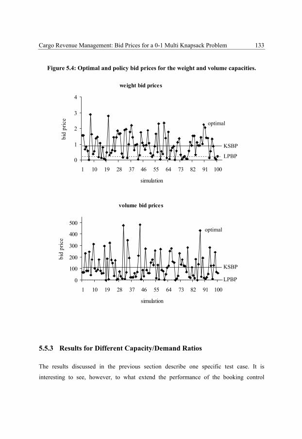
143
Cargo Revenue Management: Bid Prices for a 0-1 Multi Knapsack Problem 133
Figure 5.4: Optimal and policy bid prices for the weight and volume capacities.
5.5.3 Results for Different Capacity/Demand Ratios
The results discussed in the previous section describe one specific test case. It is
interesting to see, however, to what extend the performance of the booking control
volume bid prices
0
100
200
300
400
500
1 10 19 28 37 46 55 64 73 82 91 100
simulation
bid
pric
e
KSBP
LPBP
optimal
weight bid prices
0
1
2
3
4
1 10 19 28 37 46 55 64 73 82 91 100
simulation
bid
pric
e
KSBP
LPBP
optimal

144
Chapter 5 134
policies is influenced by the set-up of the test case. In this section we show results for
some different values for the capacity/demand ratios. We do this by varying the capacity
levels while keeping the demand as it is. We define the weight and volume capacities as a
percentage of the average demand and shift them from 0.1 to 1.5. We note that, in this
section, we only use 10 demand realizations for each decision of the dynamic
approximation scheme as opposed to 100 in the previous section. This reduces the
computation time of the many results that we generate in this section. In Chapter 3 we
have seen that this did not reduce the performance of the randomization technique much
for the test case considered there. Tests show that this also holds in this test case. Figure
5.5 shows the profit of the two bid-price policies and the dynamic approximation scheme
relative to the ex-post optimal profit for varying values for the weight capacity while
keeping the volume capacity fixed at 0.7 and for varying values of the volume capacity
while keeping the weight capacity fixed at 0.6. Each point reflects the average
performance of the policy over 100 simulated demand sequences.
Figure 5.5: Performance of the booking control policies while varying one of the capacity/demand ratios.
fixed volume capacity
0
20
40
60
80
100
0.1 0.3 0.5 0.7 0.9 1.1 1.3 1.5
weight capacity
% o
f ex-
post
opt
imal
LPBPKSBPDAS
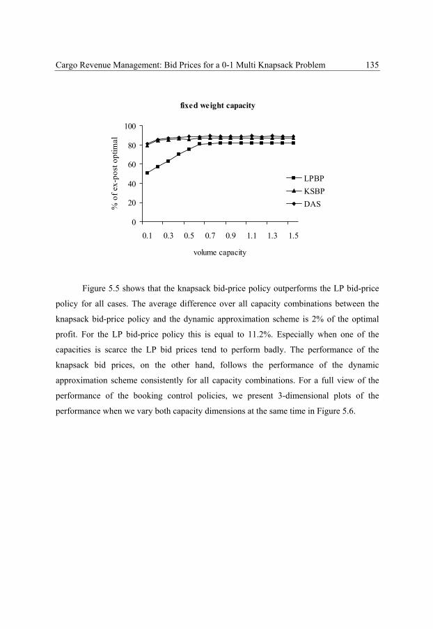
145
Cargo Revenue Management: Bid Prices for a 0-1 Multi Knapsack Problem 135
fixed weight capacity
0
20
40
60
80
100
0.1 0.3 0.5 0.7 0.9 1.1 1.3 1.5
volume capacity
% o
f ex-
post
opt
imal
LPBPKSBPDAS
Figure 5.5 shows that the knapsack bid-price policy outperforms the LP bid-price
policy for all cases. The average difference over all capacity combinations between the
knapsack bid-price policy and the dynamic approximation scheme is 2% of the optimal
profit. For the LP bid-price policy this is equal to 11.2%. Especially when one of the
capacities is scarce the LP bid prices tend to perform badly. The performance of the
knapsack bid prices, on the other hand, follows the performance of the dynamic
approximation scheme consistently for all capacity combinations. For a full view of the
performance of the booking control policies, we present 3-dimensional plots of the
performance when we vary both capacity dimensions at the same time in Figure 5.6.
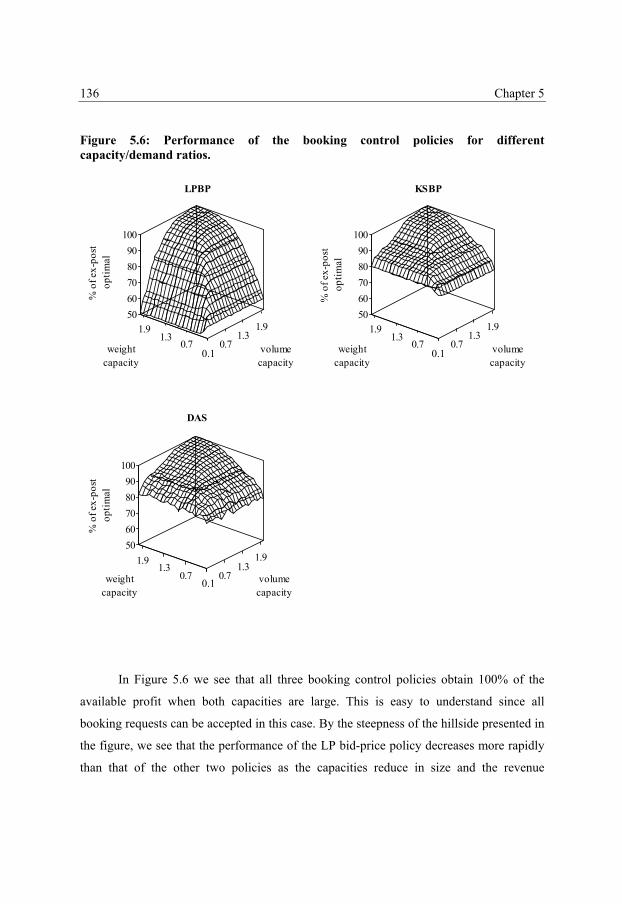
146
Chapter 5 136
Figure 5.6: Performance of the booking control policies for different capacity/demand ratios.
In Figure 5.6 we see that all three booking control policies obtain 100% of the
available profit when both capacities are large. This is easy to understand since all
booking requests can be accepted in this case. By the steepness of the hillside presented in
the figure, we see that the performance of the LP bid-price policy decreases more rapidly
than that of the other two policies as the capacities reduce in size and the revenue
0.10.7
1.31.9
0.10.7
1.31.9
5060708090
100
% o
f ex-
post
op
timal
volume capacity
weight capacity
LPBP
0.10.7
1.31.9
0.10.7
1.31.9
5060708090
100
% o
f ex-
post
op
timal
volume capacity
weight capacity
KSBP
0.10.7
1.31.9
0.10.7
1.31.9
5060708090
100
% o
f ex-
post
op
timal
volume capacity
weight capacity
DAS
0.1
0.1
0.1

147
Cargo Revenue Management: Bid Prices for a 0-1 Multi Knapsack Problem 137
management decision becomes more important. Note also that the performance of the
dynamic approximation scheme is more volatile than those of the bid-price policies. The
dynamic approximation scheme adapts itself to the situation at hand. This generally leads
to higher profits but also to a more variable kind of decision making. The bid-price
policies keep to a fixed policy that is set beforehand and that produces approximately the
same results every time it is applied.
5.6 Summary and Conclusion
Cargo revenue management differs from passenger revenue management in a number of
ways. Passengers generally belong to one of a limited number of booking classes and all
take up one seat of the total seat capacity. Cargo shipments, on the other hand, are unique
in profit, weight and volume. This means that traditional revenue management techniques
originally constructed for the passenger problem cannot be used for the cargo revenue
management problem. Instead, we formulate the problem as a 0-1 multi-dimensional on-
line knapsack problem. This formulation is capable to include a network of flights. As for
the passenger problem, we show that a bid-price acceptance policy is asymptotically
optimal if demand and capacity increase proportionally and the bid prices are set correctly.
We provide a polynomial time algorithm to obtain optimal bid prices for a given demand
sequence. Bid prices for on-line use can be constructed by taking the average bid-price
values over a number of simulated demand sequences.
A test case based on insights obtained from actual flight data, shows that the
knapsack bid prices outperform the commonly used LP bid prices for every situation that
we consider. Further, the performance of the knapsack bid prices closely follows the
performance of a dynamic approximation scheme that we formulate. Such a dynamic
approximation scheme is generally not considered to be useful in practice, but can give an
indication of how well an on-line policy can optimally perform. Bid prices, on the other
hand, are very practical and are already widely used for both passenger and cargo revenue
management.

148
Chapter 5 138
The cargo revenue management problem as we formulate it in this study is largely
how we encountered it in practice. However, some extensions to the problem that would
be worthwhile to examine still remain. First of all, we excluded the overbooking problem
from our study. Overbooking plays an important role in cargo transportation. For cargo,
the question is not so much whether or not a booked shipment shows up, but how much
the actual weight and volume will deviate from the requested quantities. Overbooking
decisions are usually made alongside revenue management decision but it would be
interesting to combine the two. Further, as Kasilingam (1996) points out, cargo can be
shipped among different routes as long as it arrives at its destination on time. Extending
the model to take into account the routing of a cargo shipment raises a lot of opportunities
for the company. Finally, the allocation of the cargo capacity over the long-term contracts
and the spot sales would also make an interesting topic for further research. Until now this
has largely been a managerial decision. Simulation studies similar to those presented in
this paper can be used to estimate the profit that can be generated when a certain amount
of capacity is made available for the spot sales. This way, the certainty of a long-term
contract can be better evaluated against the additional profit that can possibly be generated
by the spot sales.

149
Chapter 6 Summary and Conclusion
In this thesis we studied new features and models in revenue management. Revenue
management has grown into one of the most successful OR applications to date. Although
multiple definitions of revenue management exist, we mainly focus on the problem for
which it is commonly known. This is to sell a fixed and perishable capacity as profitable
as possible by selecting the right customers to sell to. As discussed in the introduction, this
can be done by either quantity-based controlling of the sales or price-based controlling of
the sales. In this thesis we use quantity-based techniques. By doing so, we stay close to the
techniques used in practice for the problems that we consider. Price-based methods would
result in different data requirements and more complicated models for these specific
problems.
Each chapter in this thesis studies a different revenue management application. In
Chapter 2 we extensively discuss the well-known airline revenue management problem.
Revenue management originates from the airline industry and the airline revenue
management problem still is the prototype for which a revenue management problem is
known. In fact, most other revenue management applications make use of the solution
techniques developed for the airline industry. By discussing the airline problem, we
provide an overview of the general problem with its assumptions, difficulties and solution
150
Chapter 6 140
techniques for most revenue management problems. In Chapter 2 we introduce and
discuss the two most popular booking control policies currently used in revenue
management: bid prices and booking limits. Both policies have their advantages and
disadvantages. However, both policies can be shown to be asymptotically optimal and are
easy to use in practice. Further, we distinguish solution methods for a single flight and a
network of flights. The latter are preferred by most airlines since they take into account
the combinatorial effects that occur when passengers make use of multiple connecting
flights to reach their destination. However, we also show that doing so drastically
complicates the model.
A number of the solution techniques discussed in Chapter 2 are applied to the hotel
industry in Chapter 3. Hotel revenue management resembles the airline revenue
management problem. The main difference between the two problems is the fact that the
combinatorial effects differ. In the airline problem the combinatorial effects are caused by
the different flights that a passenger can use to reach his/her destination. In the hotel
problem the combinatorial effects are caused by the overlapping stays when guests stay in
the hotel for multiple days. This means that the overlap faced by a hotel does not end at a
pre-specified point in time, but goes on without end. Our contribution in Chapter 3 is
twofold. First, we provide a means to capture the effect of the overlapping stays by a
rolling horizon of overlapping decision periods. Second, unlike previous studies we apply
models to the hotel revenue management problem that take into account the stochastic
nature of demand. We provide two methods to do this. The first is to apply a
randomization technique to the bid-price policy. The second is to formulate a stochastic
mathematical programming model to construct bid prices and booking limits. The booking
control policies are tested in a realistic test case. The results show that the randomized bid
prices outperform all other policies. However, this policy can be computationally
cumbersome. Booking limits provide better results than bid prices when both policies are
based on a deterministic mathematical programming model. The performance of the
booking-limit policy is not improved when the stochastic model is used. The bid prices, on
the other hand, greatly benefit from the use of the stochastic model and are able to obtain
better results than both the deterministic and stochastic booking limits. However, the
151
Summary and Conclusion 141
performance of the stochastic bid prices depends greatly on the demand discretization
used in the underlying mathematical programming model, which adds an unwanted risk to
applying the booking control policy in practice.
In Chapter 4 we return to the airline revenue management problem. In this chapter
we relax the fixed capacity assumption often thought essential for revenue management.
We do this by considering planes with convertible seats. A row of these seats can be
converted from five business seats to six economy class seats and vice versa. This offers
the airline company the opportunity to adjust the configuration of the plane to the demand
at hand. We formulate a mathematical programming model to take this shifting of the
capacity into account. This model is also extended to include cancellations and
overbooking. We present a dynamic approximation scheme for the optimal control policy
based on the mathematical programming model. The stochastic nature of demand is
accounted for by randomizing the acceptance scheme over a number of simulated demand
realizations. In order to evaluate the revenue potential of the shifting capacity opportunity,
we construct a realistic test case in which three consecutive flights with different demand
patterns are flown by the same plane. The results show that the revenue potential created
by the convertible seats is considerable even when the capacity configuration of the plane
is adjusted only once before the booking period starts. When the shifting capacity
opportunity is taken into account continuously during the booking process the revenues
can be further improved, especially when the dynamic approximation scheme is improved
by randomization. The same results are obtained when cancellations and overbooking are
taken into account. It is interesting to note, however, that one passenger can block a whole
row from converting from the business to the economy class or vice versa. Therefore,
when the shifting capacity opportunity is considered continuously, booking requests can
be turned into denied boardings intentionally even when the booking process has not
ended yet.
Finally, in Chapter 5 we consider revenue management for cargo transportation.
The fundamental difference between cargo and passenger revenue management, is that
cargo shipments are uniquely defined by their profit, weight and volume whereas
passengers generally belong to one of a limited number of price classes. In other studies

152
Chapter 6 142
on cargo revenue management (see: Kasilingam (1996) and Karaesmen (2001)) the cargo
shipments are categorized into classes such that standard revenue management techniques
developed for passenger revenue management can be applied. Unlike these studies, we
treat the cargo shipments as the unique items they are. This results in a 0-1 decision
problem. Since a cargo shipment can use multiple connecting flights to reach its
destination and the accept/deny decision has to be made as the booking request occurs, we
model the problem as a 0-1 multi-dimensional on-line knapsack problem. We show that a
bid-price acceptance policy is asymptotically optimal if demand and capacity increase
proportionally and the bid prices are set correctly. We present a polynomial time
algorithm to obtain optimal bid prices for a given set of booking requests and use this to
construct a booking control policy. A realistic test case shows that our knapsack bid prices
perform better than traditional LP-based bid prices as known for passenger revenue
management. Further, the performance of the knapsack bid prices closely follows the
performance of a computational cumbersome dynamic approximation scheme that we
formulate.
In this thesis we have extended hotel, airline and cargo revenue management
problems for new features such as a rolling horizon, convertible seats and unique booking
requests. We provide mathematical models that incorporate these features and derive
booking control policies based on those models. We test the performance of the booking
control policies in a simulated environment. Unlike most other revenue management
studies, we put a lot of effort in testing the ways to account for the stochastic nature of
demand in the models. We do this by formulating stochastic mathematical programming
models or by randomization techniques. Especially the latter provides an improvement of
the performance of the policies. However, it also increases the computation times. In some
studies, we also develop dynamic approximation schemes for the optimal control policy.
These dynamic approximation schemes are generally not considered to be useful in
practice because of the on-line computation time involved. However, they do provide an
approximation of the optimal performance of an on-line policy. The bid-price and
booking-limit booking control policies that we present, however, are very well suited for
practical use.

153
Summary and Conclusion 143
Many of the studies performed in this thesis come forth from questions raised by
revenue management practitioners. Also the test cases that we construct are chosen to
reflect realistic environments. This means that the results presented in this thesis provide
useful insights for practitioners and can be used to further develop and extend revenue
management techniques in practice.

154
155
Nederlandse Samenvatting (Summary in Dutch)
Bedrijven die bederfelijke goederen verkopen, zijn vaak genoodzaakt om een vaste
capaciteit van hun product te verkopen binnen een gegeven tijdsperiode. Indien de markt
gekarakteriseerd wordt door klanten die bereid zijn om verschillende prijzen te betalen
voor het product, is het vaak mogelijk om met behulp van product differentiatie
verschillende klantsegmenten tegelijkertijd te bedienen. Dit heeft als gevolg dat hetzelfde
product tegen verschillende prijzen kan worden verkocht. Voorbeelden hiervan zijn het
hanteren van verschillende prijzen op verschillende tijdstippen of voor verschillende
service niveaus. Wanneer er verschillende prijzen worden gehanteerd voor hetzelfde
product moet echter voorkomen worden dat dit ten koste gaat van de opbrengst doordat te
veel klanten ervoor kiezen om het product voor een lage prijs te kopen. Het is derhalve
belangrijk om de klantsegmenten voldoende te differentiëren en beslissingen te maken
omtrent welk gedeelte van de capaciteit wordt verkocht in elk prijssegment. Hierbij is het
zaak om niet te veel producten te verkopen voor een lage prijs, maar tegelijkertijd ook te
voorkomen dat producten die tegen een hogere prijs worden aangeboden, onverkocht
blijven. Hoe de capaciteit te verdelen over de verschillende prijssegmenten zodat de
opbrengst maximaal is, staat algemeen bekend als het revenue management probleem.
Revenue management komt voort uit de luchtvaart industrie, waar al lange tijd
verschillende prijsklassen worden aangeboden op een vlucht. De prijs die wordt betaald

156
Nederlandse Samenvatting 146
voor een ticket hangt veelal af van eigenschappen zoals: het tijdstip van boeken, de ticket
opties of het opnemen van een zaterdag overnachting in het verblijf. Dit zijn geen
eigenschappen die de prijs van een boeking hoeven te beïnvloeden, maar die wel worden
aangegrepen door de luchtvaartmaatschappij om het product te differentiëren en derhalve
verschillende prijsklassen te kunnen hanteren voor hetzelfde product. Andere bekende
toepassingen van revenue management zijn onder andere te vinden bij hotels, spoorwegen,
vracht vervoer en auto verhuur bedrijven. Dit proefschrift richt zich op de wiskundige
modellen die het maken van revenue management beslissingen ondersteunen. Deze
modellen zijn erop gericht de aanwezige capaciteit op de juiste manier beschikbaar te
stellen aan de verschillende prijssegmenten zodat de verwachte opbrengst maximaal is.
Elk hoofdstuk behandeld een andere toepassing van revenue management en geeft een
analyse van de beslissingsondersteunende modellen die daarvoor gebruikt kunnen worden.
In hoofdstuk 2 bespreken we het revenue management probleem zoals bekend in
de luchtvaart industrie. Het luchtvaart probleem staat bekend als het prototype revenue
management probleem. Vele andere revenue management toepassingen zijn afgeleid van
het luchtvaart probleem en met het bespreken van deze toepassing geven we derhalve ook
een overzicht van de aannamen, moeilijkheden en oplossingsmethoden voor vele andere
toepassingen. In dit hoofdstuk introduceren we ook de twee meest populaire technieken
om boekingen te controleren: ‘bid prices’ en ‘booking limits’. Een bid price kan worden
geïnterpreteerd als een minimaal te accepteren prijs voor een product. Door deze over de
tijd te fluctueren kunnen op verschillende tijdstippen verschillende prijsklassen open en
dicht worden verklaart. Booking limits daarentegen beperken het aantal boekingen dat
geaccepteerd kunnen worden in elke prijsklasse. Beide technieken hebben zo hun voor- en
nadelen. Echter, beide technieken zijn zeer praktisch in het gebruik en zijn asymptotisch
optimaal. Verder maken we onderscheid tussen technieken voor enkele vluchten en voor
een netwerk van vluchten. De laatstgenoemde technieken houden rekening met de
combinatorische aspecten die geïntroduceerd worden in het probleem wanneer passagiers
gebruik maken van meerdere vluchten om tot hun bestemming te geraken. Dit is
wenselijk, maar compliceert het onderliggende model aanzienlijk.

157
Summary in Dutch 147
Een aantal van de wiskundige modellen die we bespreken in hoofdstuk 2 voor de
luchtvaart, passen we in hoofdstuk 3 toe in de hotel industrie. Hotel revenue management
heeft veel weg van het bekende luchtvaart revenue management probleem. Het
voornaamste verschil is dat de combinatorische effecten verschillen. In het luchtvaart
probleem worden de combinatorische effecten veroorzaakt doordat passagiers meerdere
vluchten kunnen gebruiken om tot hun bestemming te geraken. In het hotel probleem
worden de combinatorische effecten veroorzaakt door de overlapping die kan bestaan
tussen de verblijven van gasten die meerdere dagen in het hotel verblijven. Waar de
combinatorische effecten in de luchtvaart beperkt zijn tot een gelimiteerd aantal vluchten,
kunnen de combinatorische effecten voor een hotel tot in het oneindige doorlopen. In
hoofdstuk 3 leveren we twee bijdragen aan de bestaande literatuur. Ten eerste tonen we
aan hoe de effecten van de overlappende verblijven op te nemen in een model met behulp
van een rollende horizon van beslissingsperioden. Ten tweede passen we, in tegenstelling
tot andere studies in de hotel industrie, modellen toe die de stochasticiteit van de vraag in
ogenschouw nemen. Dit laatste doen we op twee manieren. In de eerste plaats door
gemiddelde bid-price waarden te nemen over meerdere willekeurige trekkingen uit de
vraagverdeling. En in de tweede plaats door een stochastisch mathematisch
programmerings model te definiëren op basis waarvan bid prices en booking limits
kunnen worden bepaald. We testen de verschillende methoden in een realistische test
omgeving en vergelijken de resultaten met die van deterministische bid prices en booking
limits. Daaruit blijkt dat de eerste methode om de bid prices te verbeteren tot een sterke
verbetering van de prestaties leidt. Echter, deze methode is rekenkundig zeer intensief. Het
stochastische programmerings model leidt ook tot een verbetering van de bid-price
methode alhoewel deze prestaties erg afhankelijk zijn van de benadering van de
vraagverdeling in het model. Het model leidt niet tot een verbetering van de booking
limits methode.
In hoofdstuk 4 keren we terug naar het luchtvaart revenue management probleem.
In dit hoofdstuk laten we echter de aanname van een vaste capaciteit los. We doen dit door
vliegtuigen te beschouwen die voorzien zijn van zogeheten converteerbare stoelen. Een rij
van deze stoelen kan omgezet worden van vijf business klasse stoelen naar zes economy

158
Nederlandse Samenvatting 148
klasse stoelen en andersom. Dit bied de luchtvaart maatschappij de mogelijkheid om de
configuratie van het vliegtuig aan te passen aan de vraag van het moment. We formuleren
een mathematisch programmerings model om het verschuiven van de capaciteit op te
nemen in het beslissingsprobleem. We breiden dit model tevens uit om annuleringen en
overboeking in ogenschouw te nemen. In dit hoofdstuk gebruiken we geen bid prices of
booking limits, maar een dynamische benaderingsmethode van de optimale strategie. Om
te corrigeren voor de stochasticiteit van de vraag, wordt de methode verbeterd aan de hand
van willekeurige trekkingen uit de vraagverdeling. Om na te gaan wat de potentiële extra
opbrengst is van de converteerbare stoelen, definiëren we een realistische test case waarin
drie opeenvolgende vluchten, die elk een ander vraagpatroon hebben, worden gevlogen
door hetzelfde vliegtuig. De resultaten geven aan dat de potentiële extra opbrengst van de
converteerbare stoelen aanzienlijk is, zelfs wanneer de configuratie van het vliegtuig voor
elke vlucht voor het begin van het boekingsproces wordt bepaald. Wanner de configuratie
gedurende het boekingsproces kan worden aangepast, is de potentiële extra opbrengst nog
hoger.
Tenslotte beschouwen we in hoofdstuk 5 revenue management voor vrachtvervoer.
Het fundamentele verschil tussen revenue management voor vracht en passagiers is dat
een vracht uniek gedefinieerd wordt door zijn winstgevendheid, gewicht en omvang. Een
passagier behoort daarentegen tot één van een gelimiteerd aantal prijsklassen, waarin elke
passagier gelijk is. In andere studies op het gebied van revenue management voor
vrachtvervoer, worden de vrachten onderverdeeld in categorieën om zodoende de
standaard revenue management technieken, ontwikkeld voor passagiers, toe te kunnen
passen. In tegenstelling tot deze studies beschouwen wij de vrachten daadwerkelijk als
uniek geïdentificeerd. Dit heeft een 0-1 beslissingsprobleem als gevolg. Omdat ook
vrachten meerdere vluchten kunnen gebruiken om tot hun bestemming te komen,
formuleren we het probleem als een 0-1 multi-dimensionaal on-line knapzak probleem.
We tonen aan dat een bid-price strategie ook voor dit probleem asymptotisch optimaal is
wanneer de capaciteit en de vraag proportioneel toenemen en de bid prices juist zijn
gekozen. We leveren een algoritme dat in polynomische tijd een optimale set van bid
prices construeert voor een gegeven set van vrachten. Tevens geven we aan hoe dit
159
Summary in Dutch 149
algoritme kan worden gebruikt om bid prices te creëren die gebruikt kunnen worden
gedurende het boekingsproces. Een realistische test case wijst uit dat onze knapzak bid
prices beter presteren dan bid prices zoals traditioneel berekend voor passagiers revenue
management.
In dit proefschrift breiden we hotel, luchtvaart en vrachtvervoer revenue
management problemen uit met nieuwe eigenschappen zoals een rollende horizon,
converteerbare stoelen en unieke boekingen. We geven wiskundige modellen die deze
eigenschappen opnemen en leiden van deze modellen beslissingsmethoden af die gebruikt
kunnen worden om het accepteren van de boekingen te beheersen. We testen de prestaties
van de verschillende beslissingsmethoden in een gesimuleerde omgeving. In tegenstelling
tot de meeste andere revenue management studies, besteden we veel aandacht aan het
opnemen van de stochasticiteit van de vraag in de modellen. Ook ontwikkelen we in
enkele gevallen dynamische benaderingsmethoden voor de optimale strategie. De meeste
studies in dit proefschrift zijn probleemstellingen die direct voortkomen uit de praktijk.
Tevens zijn de test cases dusdanig gekozen dat ze de werkelijkheid weergeven. Dit houdt
in dat de resultaten die we presenteren in dit proefschrift nuttige inzichten verschaffen
voor de praktijk en gebruikt kunnen worden om revenue management modellen en
technieken verder te ontwikkelen en uitbreiden.

160
161
Bibliography
Algers, S. and Besser, M. (2001), Modeling Choice of Flight and Booking Classes: A
Study using Stated Preferences and Revealed Preference Data, International
Journal of Services Technology and Management, 2, 28-45. Andersson, S.E. (1998), Passenger Choice Analysis for Seat Capacity Control: A Pilot
Project in Scandinavian Airlines, International Transaction in Operational
Research, 5, 471-486. Baker, T.K. and Collier, D.A. (1999), A Comparative Revenue Analysis of Hotel Yield
Management Heuristics, Decision Sciences, 30, 239-263. Beckmann, M.J. (1958), Decision and Team Problems in Airline Reservations,
Econometrica, 26, 134-145. Bell, P.C. (1998), Revenue Management: That’s the Ticket, OR/MS Today, April Issue,
28. Belobaba, P.P. (1987), Airline Yield Management: An Overview of Seat Inventory
Control, Transportation Science, 21, 63-73. Belobaba, P.P. and Farkas, A. (1999), Yield Management Impacts on Airline Spill
Estimation, Transportation Science, 33, 217-232.

162
Bibliography 152
Belobaba, P.P. and Weatherford, L.R. (1996), Comparing Decision Rules that incorporate
Customer Diversion in Perishable Asset Revenue Management Situations,
Decision Sciences, 27, 343-363. Berge, M.E. and Hopperstad, C.A. (1993), Demand Driven Dispatch: A Method for
Dynamic Aircraft Capacity Assignment, Models and Algorithms, Operations
Research, 41, 153-168. Bertsimas, D.J. and de Boer, S.V. (2001), A Stochastic Booking Limit Policy for Airline
Network Revenue Management, Working Paper, Operations Research Center,
Massachusetts Institute of Technology, Cambridge, MA. Bertsimas, D.J. and Popescu, I. (2003), Revenue Management in a Dynamic Network
Environment, Transportation Science, 37, 257-277. Bitran, G.R. and Caldentey, R. (2003), An Overview of Pricing Models for Revenue
Management, Manufacturing and Service Management, 5, 203-229. Bitran, G.R. and Gilbert, S.M. (1996), Managing Hotel Reservations with Uncertain
Arrivals, Operations Research, 44, 35-49. Bitran, G.R. and Mondschein, S. (1995), An Application of Yield Management to the
Hotel Industry Considering Multiple Day Stays, Operations Research, 43, 427-
443. Bodily, S.E. and Weatherford, L.R. (1995), Perishable Asset Revenue Management:
Generic and Multi-Price Yield Management with Diversion, Omega International
Journal of Management Science, 23, 173-185. Brumelle, S.L. and McGill, J.I. (1993), Airline Seat Allocation with Multiple Nested Fare
Classes, Operations Research, 41, 127-137.
163
Bibliography 153
Brumelle, S.L., McGill, J.I., Oum, T.H., Sawaki, K. and Tretheway, M.W. (1990),
Allocation of Airline Seats between Stochastically Dependent Demands,
Transportation Science, 24, 183-192. Brumelle, S.L. and Walczak, D. (2003), Dynamic Airline Revenue Management with
Multiple Semi-Markov Demand, Operations Research, 51, 137-148. Chatwin, R.E. (2000), Optimal Dynamic Pricing of Perishable Products with Stochastic
Demand and a Finite Set of Prices, European Journal of Operational Research,
125, 149-174. Chen, V.C.P., Gűnther, D. and Johnson, E.L. (1998), A Markov Decision Problem Based
Approach to the Airline YM Problem, Working Paper, The Logistics Institute,
Georgia Institute of Technology, Atlanta, GA. Ciancimino, A., Inzerillo, G., Lucidi, S. and Palagi, L. (1999), A Mathematical
Programming Approach for the Solution of the Railway Yield Management
Problem, Transportation Science, 33, 168-181. Cooper, W.L. (2002), Asymptotic Behavior of an Allocation Policy for Revenue
Management, Operations Research, 50, 720-727. Cooper, W.L., Homem-de-Mello, T. and Kleywegt, A.J. (2004), Models of the Spiral-
Down Effect in Revenue Management, Working Paper, Department of Mechanical
Engineering, University of Minnesota, MN. Cross, R.G. (1997), Revenue Management: Hardcore Tactics for Market Domination,
Broadway Books, New York, NY. Curry, R.E. (1990), Optimal Airline Seat Allocation with Fare Classes Nested by Origins
and Destinations, Transportation Science, 24, 193-204.
164
Bibliography 154
De Boer, S.V., Freling, R. and Piersma, N. (2002), Stochastic Programming for Multiple-
Leg Network Revenue Management, European Journal of Operational Research,
137, 72-92. Feng, Y.Y. and Gallego, G. (1995), Optimal Starting Times for End-Of-Season Sales and
Optimal Stopping-Times for Promotional Fares, Management Science, 41, 1371-
1391. Feng, Y.Y. and Gallego, G. (2000), Perishable Asset Revenue Management with
Markovian Time Dependent Demand Intensities, Management Science, 46, 941-
956. Feng, Y.Y. and Xiao, B. (2000a), A Continuous-Time Yield Management Model with
Multiple Prices and Reversible Price Changes, Management Science, 46, 644-657. Feng, Y.Y. and Xiao, B. (2000b), Optimal Policies of Yield Management with Multiple
Predetermined Prices, Operations Research, 48, 332-343. Gallego, G. and van Ryzin, G.J. (1994), Optimal Dynamic Pricing of Inventories with
Stochastic Demand over Finite Horizons, Management Science, 40, 999-1020. Gallego, G. and van Ryzin, G.J. (1997), A Multiproduct Dynamic Pricing Problem and its
Applications to Network Yield Management, Operations Research, 45, 24-41. Garey, M.R. and Johnson, D.S. (1979), Computers and Intractability: A Guide to the
Theory of NP-Completeness, Freeman, San Francisco, CA. Geraghty, M.K. and Johnson, E. (1997), Revenue Management Saves National Car
Rental, Interfaces, 27, 107-127. Glover, F., Glover, R., Lorenzo, J. and McMillan, C. (1982), The Passenger Mix Problem
in the Scheduled Airlines, Interfaces, 12, 73-79.

165
Bibliography 155
Goldman, P., Freling, R., Pak, K. and Piersma, N. (2002), Models and Techniques for
Hotel Revenue Management using a Rolling Horizon, Journal of Revenue and
Pricing Management, 1, 207-219. Karaesmen, I. (2001), Three Essays in Revenue Management, Ph.D. Thesis, Graduate
School of Business, Columbia University, New York, NY. Kasilingam, R.G. (1996), Air Cargo Revenue Management: Characteristics and
Complexities, European Journal of Operational Research, 96, 36-44. Kleywegt, A.J. (2001), An Optimal Control Problem of Dynamic Pricing, Working Paper,
School of Industrial and Systems Engineering, Georgia Institute of Technology,
Atlanta, GA. Kleywegt, A.J. and Papastavrou, J.D. (1998), The Dynamic and Stochastic Knapsack
Problem, Operations Research, 46, 17-35. Kleywegt, A.J. and Papastavrou, J.D. (2001), The Dynamic and Stochastic Knapsack
Problem with Random Sized Items, Operations Research, 49, 26-41. Kraft, E.R., Srikar, B.N. and Philips, R.L. (2000), Revenue Management in Railroad
Applications, Transportation Quarterly, 54, 157-176. Lautenbacher, C.J. and Stidham jr., S. (1999), The Underlying Markov Decision Process
in the Single-Leg Airline Yield Management Problem, Transportation Science, 33,
136-146. Lee, T.C. and Hersh, M. (1993), A Model for Dynamic Airline Seat Inventory Control
with Multiple Seat Bookings, Transportation Science, 27, 252-265. Lenstra, A.K., Lenstra, J.K., Rinnooy Kan, A.H.G. and Wansbeek, T.J. (1982), Two Lines
Least Squares, Annals of Discrete Mathematics, 16, 201-211.
166
Bibliography 156
Liang, Y. (1999), Solution to the Continuous Time Dynamic Yield Management Model,
Transportation Science, 33, 117-123. Listes, O. and Dekker, R. (2002), A Scenario Aggregation Based Approach for
Determining a Robust Airline Fleet Composition, Econometric Institute Report EI
2002-17, Erasmus University Rotterdam, The Netherlands. Littlewood, K. (1972), Forecasting and Control of Passenger Bookings, In Proceedings of
the Twelfth Annual AGIFORS Symposium, Nathanya, Israel. Maglaras, C. and Meissner, J. (2004), Dynamic Pricing Strategies for Multi-Product
Revenue Management Problems, Working Paper, Columbia Business School,
Columbia University, New York, NY. McGill, J.I. and van Ryzin, G.J. (1999), Revenue Management: Research Overview and
Prospects, Transportation Science, 33, 233-256. Pak, K. and Dekker, R. (2004), Cargo Revenue Management: Bid Prices for a 0-1 Multi
Knapsack Problem, Econometric Institute Report EI 2004-26, Erasmus University
Rotterdam, The Netherlands. Pak, K., Dekker, R. and Kindervater, G. (2003), Airline Revenue Management with
Shifting Capacity, Econometric Institute Report EI 2003-46, Erasmus University
Rotterdam, The Netherlands. Pak, K. and Piersma, N. (2002), Overview of OR Techniques for Airline Revenue
Management, Statistica Neerlandica, 56, 480-496. Papastavrou, J.D., Rajagopalan, S. and Kleywegt, A.J. (1996), The Dynamic and
Stochastic Knapsack Problem with Deadlines, Management Science, 42, 1706-
1718. Pfeifer, P.E. (1989), The Airline Discount Fare Allocation Problem, Decision Sciences,
20, 149-157.

167
Bibliography 157
Rinnooy Kan, A.H.G., Stougie, L. and Vercellis, C. (1993), A Class of Generalized
Greedy Algorithms for the Multi-Knapsack Problem, Discrete Applied
Mathematics, 42, 279-290. Robinson, L.W. (1995), Optimal and Approximate Control Policies for Airline Booking
with Sequential Nonmonotonic Fare Classes, Operations Research, 43, 252-263. Smith, B.C., Leimkuhler, J.F. and Darrow, R.M (1992), Yield Management at American
Airlines, Interfaces, 22, 8-31. Subramanian, J., Stidham jr., S. and Lautenbacher, C.J. (1999), Airline Yield Management
with Overbooking, Cancellations, and No-Shows, Transportation Science, 33, 147-
167. Talluri, K.T. and van Ryzin, G.J. (1998), An Analysis of Bid-Price Controls for Network
Revenue Management, Management Science, 44, 1577-1593. Talluri, K.T. and van Ryzin, G.J. (1999), A Randomized Linear Programming Method for
Computing Network Bid Prices, Transportation Science, 33, 207-216. Talluri, K.T. and van Ryzin, G.J. (2004a), The Theory and Practice of Revenue
Management, Kluwer Academic Publishers, Dordrecht, The Netherlands. Talluri, K.T. and van Ryzin, G.J. (2004b), Revenue Management under a general Discrete
Choice Model of Consumer Behavior, Management Science, 50, 15-33. Van Ryzin, G.J. and McGill, J.I. (2000), Revenue Management Without Forecasting or
Optimization: An Adaptive Algorithm for Determining Airline Seat Protection
Levels, Management Science, 46, 760-775. Van Ryzin, G.J. and Vulcano, G.J. (2004), Simulation-Based Optimization of Virtual
Nested Controls for Network Revenue Management, Working Paper, Graduate
School of Business, Columbia University, New York, NY.

168
Bibliography 158
Van Slyke, R. and Young, Y. (2000), Finite Horizon Stochastic Knapsacks with
Applications to Yield Management, Operations Research, 48, 155-172. Weatherford, L.R. (1995), Length of Stay Heuristics: Do They Really Make a Difference,
Cornell Hotel and Restaurant Administration Quarterly, 36, 70-79. Weatherford, L.R. and Bodily, S.E. (1992), A Taxonomy and Research Overview of
Perishable-Asset Revenue Management: Yield Management, Overbooking, and
Pricing, Operations Research, 40, 831-844. Weatherford, L.R., Bodily, S.E. and Pfeifer, P.E. (1993), Modeling the Customer Arrival
Process and Comparing Decision Rules in Perishable Asset Revenue Management
Situations, Transportation Science, 27, 239-251. Williamson, E.L. (1992), Airline Network Seat Inventory Control: Methodologies and
Revenue Impacts, Ph.D. Thesis, Flight Transportation Laboratory, Massachusetts
Institute of Technology, Cambridge, MA. Wollmer, R.D. (1986), A Hub-Spoke Seat Management Model, Company Report,
Douglas Aircraft Company, McDonnell Douglas Corporation, Long Beach, CA. Wollmer, R.D. (1992), An Airline Seat Management Model for a Single Leg Route when
Lower Fare Classes Book First, Operations Research, 40, 26-37. You, P.S. (1999), Dynamic Pricing in Airline Seat Management for Flights with Multiple
Flight Legs, Transportation Science, 33, 192-206. You, P.S. (2001), Airline Seat Management with Rejection-for-Possible-Upgrade
Decision, Transportation Research Part B, 35, 507-524. Zhao, W. and Zheng, Y.S. (2000), Optimal Dynamic Pricing for Perishable Assets with
Nonhomogeneous Demand, Management Science, 46, 375-388.

169
Bibliography 159
Zhao, W. and Zheng, Y.S. (2001), A Dynamic Model for Airline Seat Allocation with
Passenger Diversion and No-Shows, Transportation Science, 35, 80-98.

170
171
Erasmus Research Institute of Management
ERIM Ph.D. Series Research in Management
Appelman, J.H., Governance of Global Interorganizational Tourism Networks; Changing
Forms of Co-ordination between the Travel Agency and Aviation Sector, Promotors: Prof.
dr. F.M. Go & Prof. dr. B. Nooteboom, EPS-2004-036-MKT, ISBN 90-5892-060-7,
http://hdl.handle.net/1765/1199 Berens, G., Corporate Branding: The Development of Corporate Associations and their
Influence on Stakeholder Reactions, Promotor: Prof. dr. C. B. M. van Riel, EPS-2004-039-
ORG, ISBN 90 –5892–065–8, http://hdl.handle.net/1765/1273 Berghe, D.A.F., Working Across Borders: Multinational Enterprises and the
Internationalization of Employment, Promotors: Prof. dr. R.J.M. van Tulder & Prof. dr.
E.J.J. Schenk, EPS-2003-029-ORG, ISBN 90-5892-05-34, http://hdl.handle.net/1765/1041 Bijman, W.J.J., Essays on Agricultural Co-operatives; Governance Structure in Fruit and
Vegetable Chains, Promotor: Prof. dr. G.W.J. Hendrikse, EPS-2002-015-ORG, ISBN: 90-
5892-024-0, http://hdl.handle.net/1765/867 Brito, M.P. de, Managing Reverse Logistics or Reversing Logistics Management?
Promotors: Prof. dr. ir. R. Dekker & Prof. dr. M. B. M. de Koster, EPS-2004-035-LIS,
ISBN: 90-5892-058-5, http://hdl.handle.net/1765/1132 Campbell, R.A.J., Rethinking Risk in International Financial Markets, Promotor: Prof. dr.
C.G. Koedijk, EPS-2001-005-F&A, ISBN: 90-5892-008-9, http://hdl.handle.net/1765/306 Chen, Y., Labour Flexibility in China’s Companies: An Empirical Study, Promotors: Prof.
dr. A. Buitendam & Prof. dr. B. Krug, EPS-2001-006-ORG, ISBN: 90-5892-012-7,
http://hdl.handle.net/1765/307
172
Daniševská, P., Empirical Studies on Financial Intermediation and Corporate Policies,
Promotor: Prof. dr. C.G. Koedijk, EPS-2004-044-F&A, ISBN 90–5892–070–4,
http://hdl.handle.net/1765/1518 Delporte-Vermeiren, D.J.E., Improving the Flexibility and Profitability of ICT-enabled
Business Networks: An Assessment Method and Tool, Promotors: Prof.mr. dr. P.H.M.
Vervest & Prof. dr. ir. H.W.G.M. van Heck, EPS-2003-020-LIS, ISBN: 90-5892-040-2,
http://hdl.handle.net/1765/359 Dijksterhuis, M., Organizational Dynamics of Cognition and Action in the Changing
Dutch and US Banking Industries, Promotors: Prof. dr. ing. F.A.J. van den Bosch & Prof.
dr. H.W. Volberda, EPS-2003-026-STR, ISBN: 90-5892-048-8,
http://hdl.handle.net/1765/1037 Fenema, P.C. van, Coordination and Control of Globally Distributed Software Projects,
Promotor: Prof. dr. K. Kumar, EPS-2002-019-LIS, ISBN: 90-5892-030-5,
http://hdl.handle.net/1765/360 Fleischmann, M., Quantitative Models for Reverse Logistics, Promotors: Prof. dr. ir.
J.A.E.E. van Nunen & Prof. dr. ir. R. Dekker, EPS-2000-002-LIS, ISBN: 3540 417 117,
http://hdl.handle.net/1765/1044 Flier, B., Strategic Renewal of European Financial Incumbents: Coevolution of
Environmental Selection, Institutional Effects, and Managerial Intentionality, Promotors:
Prof. dr. ing. F.A.J. van den Bosch & Prof. dr. H.W. Volberda, EPS-2003-033-STR,
ISBN: 90–5892–055–0, http://hdl.handle.net/1765/1071 Fok, D., Advanced Econometric Marketing Models, Promotor: Prof. dr. P.H.B.F. Franses,
EPS-2003-027-MKT, ISBN: 90-5892-049-6, http://hdl.handle.net/1765/1035 Ganzaroli , A., Creating Trust between Local and Global Systems, Promotors: Prof. dr. K.
Kumar & Prof. dr. R.M. Lee, EPS-2002-018-LIS, ISBN: 90-5892-031-3,
http://hdl.handle.net/1765/361

173
Gilsing, V.A., Exploration, Exploitation and Co-evolution in Innovation Networks,
Promotors: Prof. dr. B. Nooteboom & Prof. dr. J.P.M. Groenewegen, EPS-2003-032-
ORG, ISBN 90-5892-05-42, http://hdl.handle.net/1765/1040 Graaf, G. de, Tractable Morality: Customer Discourses of Bankers, Veterinarians and
Charity Workers, Promotors: Prof. dr. F. Leijnse & Prof. dr. T. van Willigenburg, EPS-
2003-031-ORG, ISBN: 90–5892–051–8, http://hdl.handle.net/1765/1038 Hermans. J.M., ICT in Information Services, Use and deployment of the Dutch securities
trade, 1860-1970, Promotor: Prof. dr. drs. F.H.A. Janszen, EPS-2004-046-ORG, ISBN 90-
5892-072-0, http://hdl.handle.net/1765/1793 Heugens, P.M.A.R., Strategic Issues Management: Implications for Corporate
Performance, Promotors: Prof. dr. ing. F.A.J. van den Bosch & Prof. dr. C.B.M. van Riel,
EPS-2001-007-STR, ISBN: 90-5892-009-7, http://hdl.handle.net/1765/358 Hooghiemstra, R., The Construction of Reality, Promotors: Prof. dr. L.G. van der Tas RA
& Prof. dr. A.Th.H. Pruyn, EPS-2003-025-F&A, ISBN: 90-5892-047-X,
http://hdl.handle.net/1765/871 Jansen, J.J.P., Ambidextrous Organizations, Promotors: Prof.dr.ing. F.A.J. Van den Bosch
& Prof.dr. H.W. Volberda, EPS-2005-055-STR, ISBN 90-5892-081-X Jong, C. de, Dealing with Derivatives: Studies on the Role, Informational Content and
Pricing of Financial Derivatives, Promotor: Prof. dr. C.G. Koedijk, EPS-2003-023-F&A,
ISBN: 90-5892-043-7, http://hdl.handle.net/1765/1043 Kippers, J., Empirical Studies on Cash Payments, Promotor: Prof.dr. Ph.H.B.F. Franses,
EPS-2004-043-F&A. ISBN 90-5892-069-0, http://hdl.handle.net/1765/1520 Koppius, O.R., Information Architecture and Electronic Market Performance, Promotors:
Prof. dr. P.H.M. Vervest & Prof. dr. ir. H.W.G.M. van Heck, EPS-2002-013-LIS, ISBN:
90-5892-023-2, http://hdl.handle.net/1765/921

174
Langen, P.W. de, The Performance of Seaport Clusters; A Framework to Analyze Cluster
Performance and an Application to the Seaport Clusters of Durban, Rotterdam and the
Lower Mississippi, Promotors: Prof. dr. B. Nooteboom & Prof. drs. H.W.H. Welters, EPS-
2004-034-LIS, ISBN: 90-5892-056-9, http://hdl.handle.net/1765/1133 Le Anh, T., Intelligent Control of Vehicle-Based Internal Transport Systems, Promotors:
Prof.dr. M.B.M. de Koster & Prof.dr.ir. R. Dekker, EPS-2005-051-LIS, ISBN 90-5892-
079-8 Liang, G., New Competition; Foreign Direct Investment And Industrial Development In
China, Promotor: Prof.dr. R.J.M. van Tulder, EPS-2004-047-ORG, ISBN 90–5892–073–
9, http://hdl.handle.net/1765/1795 Loef, J., Incongruity between Ads and Consumer Expectations of Advertising, Promotors:
Prof. dr. W.F. van Raaij & Prof. dr. G. Antonides, EPS-2002-017-MKT, ISBN: 90-5892-
028-3, http://hdl.handle.net/1765/869 Mandele, L.M., van der, Leadership and the Inflection Point: A Longitudinal Perspective,
Promotors: Prof. dr. H.W. Volberda, Prof. dr. H.R. Commandeur, EPS-2004-042-STR,
ISBN 90–5892–067–4, http://hdl.handle.net/1765/1302 Meer, J.R. van der, Operational Control of Internal Transport, Promotors: Prof. dr.
M.B.M. de Koster & Prof. dr. ir. R. Dekker, EPS-2000-001-LIS, ISBN:90-5892-004-6,
http://hdl.handle.net/1765/859 Miltenburg, P.R., Effects of Modular Sourcing on Manufacturing Flexibility in the
Automotive Industry: A Study among German OEMs, Promotors: Prof. dr. J. Paauwe &
Prof. dr. H.R. Commandeur, EPS-2003-030-ORG, ISBN 90-5892-052-6,
http://hdl.handle.net/1765/1039 Mol, M.M., Outsourcing, Supplier-relations and Internationalisation: Global Source
Strategy as a Chinese Puzzle, Promotor: Prof. dr. R.J.M. van Tulder, EPS-2001-010-ORG,
ISBN: 90-5892- 014-3, http://hdl.handle.net/1765/355
175
Mulder, A., Government Dilemmas in the Private Provision of Public Goods, Promotor:
Prof. dr. R.J.M. van Tulder, EPS-2004-045-ORG, ISBN: 90-5892-071-2,
http://hdl.handle.net/1765 Muller, A.R., The Rise of Regionalism: Core Company Strategies Under The Second
Wave of Integration, Promotor: Prof. dr. R.J.M. van Tulder, EPS-2004-038-ORG, ISBN
90–5892–062–3, http://hdl.handle.net/1765/1272 Oosterhout, J. van, The Quest for Legitimacy: On Authority and Responsibility in
Governance, Promotors: Prof. dr. T. van Willigenburg & Prof.mr. H.R. van Gunsteren,
EPS-2002-012-ORG, ISBN: 90-5892-022-4, http://hdl.handle.net/1765/362 Peeters, L.W.P., Cyclic Railway Timetable Optimization, Promotors: Prof. dr. L.G. Kroon
& Prof. dr. ir. J.A.E.E. van Nunen, EPS-2003-022-LIS, ISBN: 90-5892-042-9,
http://hdl.handle.net/1765/429 Popova. V., Knowledge Discovery and Monotonicity, Promotor: Prof. dr. A. de Bruin,
EPS-2004-037-LIS, ISBN 90-5892-061-5, http://hdl.handle.net/1765/1201 Puvanasvari Ratnasingam, P., Interorganizational Trust in Business to Business E-
Commerce, Promotors: Prof. dr. K. Kumar & Prof. dr. H.G. van Dissel, EPS-2001-009-
LIS, ISBN: 90-5892-017-8, http://hdl.handle.net/1765/356 Romero Morales, D., Optimization Problems in Supply Chain Management, Promotors:
Prof. dr. ir. J.A.E.E. van Nunen & Dr. H.E. Romeijn, EPS-2000-003-LIS, ISBN: 90-
9014078-6, http://hdl.handle.net/1765/865 Roodbergen , K.J., Layout and Routing Methods for Warehouses, Promotors: Prof. dr.
M.B.M. de Koster & Prof. dr. ir. J.A.E.E. van Nunen, EPS-2001-004-LIS, ISBN: 90-
5892-005-4, http://hdl.handle.net/1765/861
176
Schweizer, T.S., An Individual Psychology of Novelty-Seeking, Creativity and Innovation,
Promotor: Prof.dr. R.J.M. van Tulder. EPS-2004-048-ORG, ISBN: 90-5892-07-71,
http://hdl.handle.net/1765/1818 Six, F.E., Trust and Trouble: Building Interpersonal Trust Within Organizations,
Promotors: Prof. dr. B. Nooteboom & Prof. dr. A.M. Sorge, EPS-2004-040-ORG, ISBN
90–5892–064–X, http://hdl.handle.net/1765/1271 Slager, A.M.H., Banking across Borders, Promotors: Prof. dr. D.M.N. van Wensveen &
Prof. dr. R.J.M. van Tulder, EPS-2004-041-ORG, ISBN 90-5892-066–6,
http://hdl.handle.net/1765/1301 Speklé, R.F., Beyond Generics: A closer look at Hybrid and Hierarchical Governance,
Promotor: Prof. dr. M.A. van Hoepen RA, EPS-2001-008-F&A, ISBN: 90-5892-011-9,
http://hdl.handle.net/1765/357 Teunter, L.H., Analysis of Sales Promotion Effects on Household Purchase Behavior,
Promotors: Prof. dr. ir. B. Wierenga & Prof. dr. T. Kloek, EPS-2002-016-ORG, ISBN: 90-
5892-029-1, http://hdl.handle.net/1765/868 Valck, K. de, Virtual Communities of Consumption: Networks of Consumer Knowledge
and Companionship, Promotors: Prof. dr. ir. G.H. van Bruggen, & Prof. dr. ir. B.
Wierenga, EPS-2005-050-MKT, ISBN 90-5892-078-X Verheul, I., Is there a (fe)male approach? Understanding gender differences in
entrepreneurship, Prof. dr. A.R. Thurik, EPS-2005-054-ORG, ISBN 90-5892-080-1 Vis, I.F.A., Planning and Control Concepts for Material Handling Systems, Promotors:
Prof. dr. M.B.M. de Koster & Prof. dr. ir. R. Dekker, EPS-2002-014-LIS, ISBN: 90-5892-
021-6, http://hdl.handle.net/1765/866 Vliet, P. van, Downside Risk and Empirical Asset Pricing, Promotor: Prof. dr. G.T. Post,
EPS-2004-049-F&A ISBN 90-5892-07-55, http://hdl.handle.net/1765/1819
177
Waal, T. de, Processing of Erroneous and Unsafe Data, Promotor: Prof. dr. ir. R. Dekker,
EPS-2003-024-LIS, ISBN: 90-5892-045-3, http://hdl.handle.net/1765/870 Wielemaker, M.W., Managing Initiatives: A Synthesis of the Conditioning and
Knowledge-Creating View, Promotors: Prof. dr. H.W. Volberda & Prof. dr. C.W.F.
Baden-Fuller, EPS-2003-28-STR, ISBN 90-5892-050-X, http://hdl.handle.net/1765/1036 Wijk, R.A.J.L. van, Organizing Knowledge in Internal Networks: A Multilevel Study,
Promotor: Prof. dr. ing. F.A.J. van den Bosch, EPS-2003-021-STR, ISBN: 90-5892-039-9,
http://hdl.handle.net/1765/347 Wolters, M.J.J., The Business of Modularity and the Modularity of Business, Promotors:
Prof. mr. dr. P.H.M. Vervest & Prof. dr. ir. H.W.G.M. van Heck, EPS-2002-011-LIS,
ISBN: 90-5892-020-8, http://hdl.handle.net/1765/920

Revenue Management: New Features and ModelsRevenue management is the art of selling a fixed and perishable
capacity of a product to those customers that generate the highest
revenue. In recent years, revenue management has gained a lot of
attention among both academics and practitioners and has grown into
one of the most successful applications of operations research. This
thesis provides an overview of revenue management techniques pre-
sented throughout the literature. More importantly, new techniques
are constructed for hotel, airline and cargo revenue management pro-
blems to account for new features such as a rolling horizon, convertible
seats and unique booking requests. Mathematical, stochastic and
dynamic programming techniques are used to construct solution
techniques which are evaluated in a simulated environment chosen in
correspondence with practitioners. The results provide useful insights
for practitioners and can be used to further develop and extend
current revenue management techniques.
Kevin Pak (1977) obtained his Master’s degree in Econometrics and
Operations Research from the Erasmus University Rotterdam in 2000.
In the same year he joined ERIM in order to carry out his doctoral
research on the subject of revenue management. Throughout the
years his work has been published in and presented at a number of
international journals and conferences. Currently, he applies his
knowledge of operations research into practice as a consultant at
ORTEC bv.
ERIMThe Erasmus Research Institute of Management (ERIM) is the
Research School (Onderzoekschool) in the field of management of the
Erasmus University Rotterdam. The founding participants of ERIM
are RSM Erasmus University and the Erasmus School of Economics.
ERIM was founded in 1999 and is officially accredited by the Royal
Netherlands Academy of Arts and Sciences (KNAW). The research
undertaken by ERIM is focussed on the management of the firm in its
environment, its intra- and inter-firm relations, and its business
processes in their interdependent connections.
The objective of ERIM is to carry out first rate research in manage-
ment, and to offer an advanced graduate program in Research in
Management. Within ERIM, over two hundred senior researchers and
Ph.D. candidates are active in the different research programs. From
a variety of academic backgrounds and expertises, the ERIM commu-
nity is united in striving for excellence and working at the forefront
of creating new business knowledge.
www.erim.eur.nl ISBN 90-5892-092-5
KEVIN PAK
Revenue Management:New Features and Models
61
KE
VIN
PA
KR
ev
en
ue
Ma
na
ge
me
nt: N
ew
Fea
ture
s an
d M
od
els
Desig
n: B
&T O
ntw
erp en
advies w
ww
.b-en
-t.nl
Print:H
aveka ww
w.h
aveka.nl
Erim - 05 omslag Pak 5/30/05 9:20 AM Pagina 1