reuse-centric programming system support of machine learning

ABSTRACT

GUAN, HUI. Reuse-Centric Programming System Support of Machine Learning. (Under the directionof Xipeng Shen and Hamid Krim.)

Modern machine learning, especially deep learning, has shown dramatic progress. Its effective

adoption, however, faces a fundamental question: how to create models that efficiently deliver

reliable predictions to meet the requirements of diverse applications running on various systems.

This thesis introduces reuse-centric optimization, a novel direction for addressing the fundamental

question. Reuse-centric optimization centers around harnessing reuse opportunities for enhancing

computing efficiency. It generalizes the reuse principle in traditional compilers to a higher level and

a larger scope through innovations in both programming systems and machine learning algorithms

and their synergy. Its exploitation of computation reuse spans across the boundaries of machine

learning algorithms, implementations, and infrastructures; the types of reuse it covers range from

pre-trained Neural Network building blocks to preprocessed results for model training and even

memory bits; the scopes of reuse it leverages go from training pipelines of deep learning to variants

of Neural Networks in ensembles; the benefits it generates include (1) up to 9X faster k-means

configurations, (2) up to 186X speedup for finding a good smaller Convolution Neural Network

(CNN), (3) up to 2X faster ensemble training with data sharing, (4) the elimination of all space cost

in protecting parameters of CNNs.

Reuse-Centric Programming System Support of Machine Learning

byHui Guan

A dissertation submitted to the Graduate Faculty ofNorth Carolina State University

in partial fulfillment of therequirements for the Degree of

Doctor of Philosophy

Electrical Engineering

Raleigh, North Carolina

2020

APPROVED BY:

Huiyang Zhou Andrew Rindos

Xipeng ShenCo-chair of Advisory Committee

Hamid KrimCo-chair of Advisory Committee

ACKNOWLEDGEMENTS

I would like to thank my Ph.D. advisor Dr. Xipeng Shen. I am very fortunate to work on my thesis

under his guidance for the last four years of my Ph.D. I have learned a lot from him including how

to find and solve a research problem, how to present the work to audiences, and how to expand the

discovery to a broader scope. I am very grateful for his visionary advice, constructive discussion,

insightful feedback, and generous support. His passion to conduct impactful research and solve

challenging problems has greatly motivated me during my Ph.D. journey and will continue to have

a profound influence on my academic career. I could not have imagined having a better advisor for

my Ph.D. study.

I would also thank my co-advisor, Dr. Hamid Krim. I received his guidance since I joined his

research lab in 2014. During the past six years, Hamid offered me invaluable advice and uncountable

comments that guide me through challenging problems. He gave me the freedom to explore various

projects. He believed in me and gave me endless support. He convinced me to take numerous math

courses for a solid math background. He mentored me with his professional expertise, brilliant

thinking, and vast patience. I feel so fortunate to have Hamid as my co-advisor.

Besides my advisors, I would like to thank the rest of my dissertation committee members

(Dr. Huiyang Zhou, Dr. Min Chi, and Dr. Andrew Rindos) for their great support and valuable

suggestions. I am thankful to Dr. Huiyang Zhou, an expert in Computer Architecture and Systems,

for his tremendous contributions to many of my research projects. I am also grateful to Dr. Min Chi

for her insightful comments on writing good research proposals and identifying promising research

topics. I also appreciate the many internship opportunities provided by Dr. Andrew Rindos at IBM

and his generous support for funding my research projects.

I would like to thank my friends and lab mates for their continued support. This dissertation

would not be possible without the intellectual contribution of Yufei Ding, Lin Ning, Randall Pittman,

Laxmikant Mokadam, and Zhen Lin. Moreover, I am thankful to Guoyang Chen, Yue Zhao, Weijie

Zhou, Zifan Nan, Guoqiang Zhang, Yuanchao Xu, Chencheng Ye, Weiqi Sun, Shuai Yang, Dong Xu,

Jou-An Chen, Lei Zhang for making my experience in the PICTure Research Group and graduate

school exciting and fun. It was a pleasure working together with them all. I would also like to thank

Xing Pan for his long-lasting support, my roommate Jie Wang for her accompany, and many other

friends for making my Ph.D. life a memorable and enjoyable experience.

It has been an honor to work with many great researchers outside of NCSU. I would like to thank

Dr. Seung-Hwan Lim and Dr. Robert Patton from Oak Ridge National Labs. I have been collaborating

with them since 2017 and was given the great opportunity to work on large-scale systems, TITAN

and SummitDev supercomputers. The collaborations result in numerous exciting ideas and fruitful

publications. I also appreciate the great help from my recommendation letter writers, Dr. Chen Ding

and Dr. Michael Carbin for my faculty job search. I am grateful of the enjoyable discussions with

them, their valuable suggestions on both research and job search, and their huge efforts in realizing

my academic dreams.

ii

Finally, I would like to give my sincere thanks to my family: Mom, Dad, and my brother. Their

encouragement went through thousands of miles from home to the US to give me courage. I could

not accomplish what I did without their love and support.

iii

TABLE OF CONTENTS

LIST OF TABLES . . . . . . . . . . . . . . . . . . . . . . . . . . . . . . . . . . . . . . . . . . . . . . . . . . . . . . . . . vi

LIST OF FIGURES . . . . . . . . . . . . . . . . . . . . . . . . . . . . . . . . . . . . . . . . . . . . . . . . . . . . . . . . vii

Chapter 1 INTRODUCTION . . . . . . . . . . . . . . . . . . . . . . . . . . . . . . . . . . . . . . . . . . . . . . 11.1 Motivation . . . . . . . . . . . . . . . . . . . . . . . . . . . . . . . . . . . . . . . . . . . . . . . . . . . . . . . 21.2 Contribution and Thesis Outline . . . . . . . . . . . . . . . . . . . . . . . . . . . . . . . . . . . . . . . 3

Chapter 2 Background . . . . . . . . . . . . . . . . . . . . . . . . . . . . . . . . . . . . . . . . . . . . . . . . . . 62.1 K-Means Clustering . . . . . . . . . . . . . . . . . . . . . . . . . . . . . . . . . . . . . . . . . . . . . . . . 72.2 Convolutional Neural Networks . . . . . . . . . . . . . . . . . . . . . . . . . . . . . . . . . . . . . . . 7

2.2.1 CNN Architectures . . . . . . . . . . . . . . . . . . . . . . . . . . . . . . . . . . . . . . . . . . . 82.2.2 CNN Pruning . . . . . . . . . . . . . . . . . . . . . . . . . . . . . . . . . . . . . . . . . . . . . . . 9

2.3 DNN Training . . . . . . . . . . . . . . . . . . . . . . . . . . . . . . . . . . . . . . . . . . . . . . . . . . . . 102.3.1 DNN Training Pipeline . . . . . . . . . . . . . . . . . . . . . . . . . . . . . . . . . . . . . . . . 112.3.2 Data-Parallel DNN Training . . . . . . . . . . . . . . . . . . . . . . . . . . . . . . . . . . . . . 11

Chapter 3 Reuse-Centric K-Means Configuration . . . . . . . . . . . . . . . . . . . . . . . . . . . . . . 133.1 Introduction . . . . . . . . . . . . . . . . . . . . . . . . . . . . . . . . . . . . . . . . . . . . . . . . . . . . . 133.2 Proposed Techniques . . . . . . . . . . . . . . . . . . . . . . . . . . . . . . . . . . . . . . . . . . . . . . . 15

3.2.1 Overview of K-Means Configuration . . . . . . . . . . . . . . . . . . . . . . . . . . . . . . 153.2.2 Overview of the Acceleration Techniques . . . . . . . . . . . . . . . . . . . . . . . . . . . 163.2.3 Reuse-Based Filtering . . . . . . . . . . . . . . . . . . . . . . . . . . . . . . . . . . . . . . . . . 173.2.4 Center Reuse . . . . . . . . . . . . . . . . . . . . . . . . . . . . . . . . . . . . . . . . . . . . . . . 203.2.5 Two-Phase Design . . . . . . . . . . . . . . . . . . . . . . . . . . . . . . . . . . . . . . . . . . . 22

3.3 Evaluations . . . . . . . . . . . . . . . . . . . . . . . . . . . . . . . . . . . . . . . . . . . . . . . . . . . . . . 253.3.1 Methodology . . . . . . . . . . . . . . . . . . . . . . . . . . . . . . . . . . . . . . . . . . . . . . . 253.3.2 Speedups on Heuristic Search . . . . . . . . . . . . . . . . . . . . . . . . . . . . . . . . . . . 263.3.3 Speedups on the Attainment of Error Surfaces . . . . . . . . . . . . . . . . . . . . . . . 283.3.4 Quality Influence of Center Reuse . . . . . . . . . . . . . . . . . . . . . . . . . . . . . . . . 313.3.5 Sensitivity Analysis and Insights . . . . . . . . . . . . . . . . . . . . . . . . . . . . . . . . . 32

3.4 Related Work . . . . . . . . . . . . . . . . . . . . . . . . . . . . . . . . . . . . . . . . . . . . . . . . . . . . . 363.5 Conclusions . . . . . . . . . . . . . . . . . . . . . . . . . . . . . . . . . . . . . . . . . . . . . . . . . . . . . . 36

Chapter 4 Composability-Based Fast CNN Pruning . . . . . . . . . . . . . . . . . . . . . . . . . . . . . 394.1 Introduction . . . . . . . . . . . . . . . . . . . . . . . . . . . . . . . . . . . . . . . . . . . . . . . . . . . . . 394.2 Composability-Based CNN Pruning: Idea and Challenges . . . . . . . . . . . . . . . . . . . . 414.3 Overview of Wootz Framework . . . . . . . . . . . . . . . . . . . . . . . . . . . . . . . . . . . . . . . . 424.4 Hierarchical Tuning Block Identifier . . . . . . . . . . . . . . . . . . . . . . . . . . . . . . . . . . . . 44

4.4.1 Optimal Tuning Block Definition Problem . . . . . . . . . . . . . . . . . . . . . . . . . . 444.4.2 Hierarchical Compression-Based Algorithm . . . . . . . . . . . . . . . . . . . . . . . . . 45

4.5 Composability-Based Pruning and Wootz Compiler . . . . . . . . . . . . . . . . . . . . . . . . . 474.5.1 Mechanisms . . . . . . . . . . . . . . . . . . . . . . . . . . . . . . . . . . . . . . . . . . . . . . . . 474.5.2 Wootz Compiler and Scripts . . . . . . . . . . . . . . . . . . . . . . . . . . . . . . . . . . . . 49

4.6 Evaluations . . . . . . . . . . . . . . . . . . . . . . . . . . . . . . . . . . . . . . . . . . . . . . . . . . . . . . 524.6.1 Experiment Settings . . . . . . . . . . . . . . . . . . . . . . . . . . . . . . . . . . . . . . . . . . 52

iv

4.6.2 Validation of the Composability Hypothesis . . . . . . . . . . . . . . . . . . . . . . . . . 544.6.3 Results of Wootz . . . . . . . . . . . . . . . . . . . . . . . . . . . . . . . . . . . . . . . . . . . . . 56


Chapter 5 Efficient Ensemble Training with Data Sharing . . . . . . . . . . . . . . . . . . . . . . . . 625.1 Introduction . . . . . . . . . . . . . . . . . . . . . . . . . . . . . . . . . . . . . . . . . . . . . . . . . . . . . 625.2 Overview of FLEET . . . . . . . . . . . . . . . . . . . . . . . . . . . . . . . . . . . . . . . . . . . . . . . . . 645.3 Resource Allocation Algorithms . . . . . . . . . . . . . . . . . . . . . . . . . . . . . . . . . . . . . . . 65

5.3.1 Problem Definition . . . . . . . . . . . . . . . . . . . . . . . . . . . . . . . . . . . . . . . . . . . 655.3.2 Complexity Analysis . . . . . . . . . . . . . . . . . . . . . . . . . . . . . . . . . . . . . . . . . . 675.3.3 Greedy Allocation Algorithm . . . . . . . . . . . . . . . . . . . . . . . . . . . . . . . . . . . . 68

5.4 Implementation . . . . . . . . . . . . . . . . . . . . . . . . . . . . . . . . . . . . . . . . . . . . . . . . . . . 735.5 Evaluations . . . . . . . . . . . . . . . . . . . . . . . . . . . . . . . . . . . . . . . . . . . . . . . . . . . . . . 75

5.5.1 Experiment Settings . . . . . . . . . . . . . . . . . . . . . . . . . . . . . . . . . . . . . . . . . . 755.5.2 End-to-End Speedups . . . . . . . . . . . . . . . . . . . . . . . . . . . . . . . . . . . . . . . . . 785.5.3 Overhead . . . . . . . . . . . . . . . . . . . . . . . . . . . . . . . . . . . . . . . . . . . . . . . . . . 80


Chapter 6 In-Place Zero-Space Memory Protection for CNN . . . . . . . . . . . . . . . . . . . . . . 836.1 Introduction . . . . . . . . . . . . . . . . . . . . . . . . . . . . . . . . . . . . . . . . . . . . . . . . . . . . . 836.2 Premises and Scopes . . . . . . . . . . . . . . . . . . . . . . . . . . . . . . . . . . . . . . . . . . . . . . . 846.3 In-Place Zero-Space ECC . . . . . . . . . . . . . . . . . . . . . . . . . . . . . . . . . . . . . . . . . . . . 85

6.3.1 WOT . . . . . . . . . . . . . . . . . . . . . . . . . . . . . . . . . . . . . . . . . . . . . . . . . . . . . 866.3.2 Full Design of In-Place Zero-Space ECC . . . . . . . . . . . . . . . . . . . . . . . . . . . . 88

6.4 Evaluations . . . . . . . . . . . . . . . . . . . . . . . . . . . . . . . . . . . . . . . . . . . . . . . . . . . . . . 896.4.1 Experiment Settings . . . . . . . . . . . . . . . . . . . . . . . . . . . . . . . . . . . . . . . . . . 896.4.2 WOT results . . . . . . . . . . . . . . . . . . . . . . . . . . . . . . . . . . . . . . . . . . . . . . . . 906.4.3 Fault injection results . . . . . . . . . . . . . . . . . . . . . . . . . . . . . . . . . . . . . . . . . 90

6.5 Related Work . . . . . . . . . . . . . . . . . . . . . . . . . . . . . . . . . . . . . . . . . . . . . . . . . . . . . 916.6 Future Directions . . . . . . . . . . . . . . . . . . . . . . . . . . . . . . . . . . . . . . . . . . . . . . . . . . 926.7 Conclusions . . . . . . . . . . . . . . . . . . . . . . . . . . . . . . . . . . . . . . . . . . . . . . . . . . . . . . 93

Chapter 7 Conclusions and Future Work . . . . . . . . . . . . . . . . . . . . . . . . . . . . . . . . . . . . . 96

BIBLIOGRAPHY . . . . . . . . . . . . . . . . . . . . . . . . . . . . . . . . . . . . . . . . . . . . . . . . . . . . . . . . . 99

v

LIST OF TABLES

Table 3.1 Data statistics. . . . . . . . . . . . . . . . . . . . . . . . . . . . . . . . . . . . . . . . . . . . . . . 26Table 3.2 Speedups on stochastic hill climbing. . . . . . . . . . . . . . . . . . . . . . . . . . . . . . 27Table 3.3 Speedups on the attainment of error surfaces. . . . . . . . . . . . . . . . . . . . . . . . 28Table 3.4 Speedup in parallel settings. . . . . . . . . . . . . . . . . . . . . . . . . . . . . . . . . . . . . 30Table 3.5 Speedups of center reuse across k with different k s t e p . . . . . . . . . . . . . . . . 34Table 3.6 Speedups of center reuse across k with different d s t e p . . . . . . . . . . . . . . . . 35Table 3.7 Speedups and distance savings for the first iteration of k-means with reuse-

based filtering across k . . . . . . . . . . . . . . . . . . . . . . . . . . . . . . . . . . . . . . . . 35

Table 4.1 Dataset statistics. . . . . . . . . . . . . . . . . . . . . . . . . . . . . . . . . . . . . . . . . . . . . 53Table 4.2 Median accuracies of default networks (init, final) and block-trained networks

(init+, final+). . . . . . . . . . . . . . . . . . . . . . . . . . . . . . . . . . . . . . . . . . . . . . . . 55Table 4.3 Speedups and configuration savings for ResNet-50 by composability-based

pruning (when 1, 4, or 16 machines are used for both baseline and composability-based methods as "#nodes" column indicates). Notations are at the tablebottom. . . . . . . . . . . . . . . . . . . . . . . . . . . . . . . . . . . . . . . . . . . . . . . . . . . . 58

Table 4.4 Speedups and configuration savings for Inception-V3 by composability-basedpruning. . . . . . . . . . . . . . . . . . . . . . . . . . . . . . . . . . . . . . . . . . . . . . . . . . . . 59

Table 4.5 Speedups by composability-based pruning with different subspace sizes. . . . 59Table 4.6 Extra speedups brought by improved tuning block definitions. . . . . . . . . . . . 60

Table 5.1 The job of different processes. . . . . . . . . . . . . . . . . . . . . . . . . . . . . . . . . . . . 64Table 5.2 Notations. . . . . . . . . . . . . . . . . . . . . . . . . . . . . . . . . . . . . . . . . . . . . . . . . . 66Table 5.3 Mean and standard deviation of the running length of DNNs in seconds. (80

GPUs, 100 DNNs) . . . . . . . . . . . . . . . . . . . . . . . . . . . . . . . . . . . . . . . . . . . . 80Table 5.4 Scheduling and checkpointing overhead. . . . . . . . . . . . . . . . . . . . . . . . . . . . 80

Table 6.1 Accuracy and weight distribution of 8-bit quantized CNN models on Ima-geNet. The percentage rows use absolute values. . . . . . . . . . . . . . . . . . . . . . 85

Table 6.2 Accuracy drop of VGG16, ResNet-16, and SqueezeNet under different memoryfault rates. . . . . . . . . . . . . . . . . . . . . . . . . . . . . . . . . . . . . . . . . . . . . . . . . . 91

vi

LIST OF FIGURES

Figure 1.1 Overview of the reuse scopes, types, and benefits of reuse-centric optimization. 2Figure 1.2 Reuse is a principle for code optimizations in compilers. . . . . . . . . . . . . . . . 2

Figure 2.1 CNN and CNN Pruning. Conv1 and Conv2 are the first two consecutiveconvolutional layers in the CNN. . . . . . . . . . . . . . . . . . . . . . . . . . . . . . . . . 8

Figure 2.2 A DNN training pipeline [Pit18]. . . . . . . . . . . . . . . . . . . . . . . . . . . . . . . . . . 10Figure 2.3 An illustration of data-parallel DNN training [Ser18]. . . . . . . . . . . . . . . . . . 11

Figure 3.1 Overview of k-means–based applications and where our three accelerationtechniques are applied. . . . . . . . . . . . . . . . . . . . . . . . . . . . . . . . . . . . . . . . 16

Figure 3.2 Illustration of how upper bound and lower bound can help avoid distancecomputation to some center c . Circles and double circles represent centersin current and previous iteration respectively, and b (x ) is the so-far nearestcenter of point x . . . . . . . . . . . . . . . . . . . . . . . . . . . . . . . . . . . . . . . . . . . . 18

Figure 3.3 Illustration of how the configuration with k = k1 can help save distancecomputation in the first iteration of another configuration with k = k2. b ′(x )is the closest center of point x when k = k1; c1, c2, c3 are the initial centersand b (x ) is the so-far nearest center of point x when k = k2. . . . . . . . . . . . . 19

Figure 3.4 Illustration of how the configuration with F1 can help save distance compu-tation in the first iteration of another configuration with F2, where b ′(x ) iscomputed from the closest center of point x in feature space F1, while c1, c2,... ck2

and b (x ) are the initial centers and the so-far nearest center of point xin feature space F2 respectively. . . . . . . . . . . . . . . . . . . . . . . . . . . . . . . . . . 20

Figure 3.5 Illustration of center reuse across k . The two graphs represent the k-meanson two configurations with k equaling three (left) and two (right) respectively.The double circles in the left graph show the three centers attained in theexploration of that configuration. These centers are grouped to get two groupcenters c ′1, c ′2, which are then used as the initial centers (marked as circles inthe right picture) for exploring the latter configuration. . . . . . . . . . . . . . . . . 22

Figure 3.6 An example of an error curve and the illustration of curve segmentation. . . . 23

vii

Figure 3.7 Approximated classification error curves from the first phase for two datasets. 24Figure 3.8 Classification error curves for two datasets. . . . . . . . . . . . . . . . . . . . . . . . . 31Figure 3.9 Center reuse across k with inc/dec k on dataset connect. acc. is short for

accumulated. . . . . . . . . . . . . . . . . . . . . . . . . . . . . . . . . . . . . . . . . . . . . . . 33Figure 3.10 Center reuse across feature sets with inc/dec d . . . . . . . . . . . . . . . . . . . . . . 34Figure 3.11 Reuse-based filtering performance on different k and different numbers of

landmarks (#lms) on adult (dim=11). . . . . . . . . . . . . . . . . . . . . . . . . . . . . . 37Figure 3.12 Reuse-based filtering performance on different k and different numbers of

landmarks (#lms) on adult (dim=59). . . . . . . . . . . . . . . . . . . . . . . . . . . . . . 38

Figure 4.1 Complementary relation with prior work for CNN pruning. Prior workshave designed heuristic criteria to quickly determine the importance of afilter [Li16; Hu16; Mol16; Luo17a], or to combine with reinforcement learn-ing for selecting the set of promising configurations [He18; Ash17]. Thiswork tries to accelerate the explorations of the remaining promising config-urations through computation reuse via composability (block pre-training)supported with a compiler-based framework. . . . . . . . . . . . . . . . . . . . . . . . 40

Figure 4.2 Overview of Wootz framework. . . . . . . . . . . . . . . . . . . . . . . . . . . . . . . . . . 42Figure 4.3 Formats for the specifications of promising subspaces (a) and pruning ob-

jectives (b). . . . . . . . . . . . . . . . . . . . . . . . . . . . . . . . . . . . . . . . . . . . . . . . 43Figure 4.4 Sequitur applies to a concatenated sequence of layers of four networks

pruned at rates: 0%, 30%, 50%. . . . . . . . . . . . . . . . . . . . . . . . . . . . . . . . . . . 46Figure 4.5 Illustration of composability-based network pruning. Eclipses are pruned

tuning blocks; rectangles are original tuning blocks; diamonds refer to theactivation map reconstruction error. Different colors of pruned tuning blockscorrespond to different pruning options. . . . . . . . . . . . . . . . . . . . . . . . . . . 49

Figure 4.6 Accuracy curves of the default and block-trained networks on dataset CUB200.Each network has 70% least important filters pruned at all convolution mod-ules. . . . . . . . . . . . . . . . . . . . . . . . . . . . . . . . . . . . . . . . . . . . . . . . . . . . . . 55

Figure 4.7 Accuracies of pruned networks of ResNet-50 after training. The model sizeof full ResNet-50 is 25.6 million. . . . . . . . . . . . . . . . . . . . . . . . . . . . . . . . . . 55

Figure 5.1 An illustration of the ensemble training pipeline in FLEET. P1 and P2 arepreprocessors and T1-T8 are trainers. There are four training groups, (T1),(T2, T3), (T4), (T5, T6, T7, T8), which train the four DNNs D1-D4 respectively.Edges indicate transfers of preprocessed images. . . . . . . . . . . . . . . . . . . . . 64

Figure 5.2 Illustration of the dataflow implementation. Two DNNs, D 1 and D 2, aretrained using four GPUs (Ranks 0-3) by two training groups, (T 1)and (T 2, T 3, T 4).T 1 and T 2 are training group masters. Sizes of QP , QT and QD are 2048 im-ages, 2048 images and 10 batches respectively. . . . . . . . . . . . . . . . . . . . . . . 74

Figure 5.3 Correlations between model size of a DNN and the training rate and thenumber of epochs until convergence. . . . . . . . . . . . . . . . . . . . . . . . . . . . . . 75

Figure 5.4 The profiled training rates (images/sec) of 100 DNNs in an ensemble withImagenet. . . . . . . . . . . . . . . . . . . . . . . . . . . . . . . . . . . . . . . . . . . . . . . . . 77

Figure 5.5 The averaged speedups over the baseline in terms of the end-to-end timefor training a 100-DNN ensemble. The error bars show the variations. . . . . . 78

Figure 5.6 Waiting time per GPU. . . . . . . . . . . . . . . . . . . . . . . . . . . . . . . . . . . . . . . . 79

viii

Figure 6.1 Large weight (beyond [−64, 63]) distributions in 8-byte (64-bit data) blocksfor SqueezeNet on ImageNet. For instance, the first bar in (a) shows that ofall the 8-byte data blocks storing weights, around 380 have a large weight atthe first byte. . . . . . . . . . . . . . . . . . . . . . . . . . . . . . . . . . . . . . . . . . . . . . . . 85

Figure 6.2 Hardware design for in-place zero-space ECC protection. . . . . . . . . . . . . . . 89Figure 6.3 Changes of the total number of large values (beyond [−64, 63]) in the first 7

positions of 8-byte (64-bit data) blocks before the throttling step during theWOT training process. . . . . . . . . . . . . . . . . . . . . . . . . . . . . . . . . . . . . . . . . 94

Figure 6.4 Accuracy curves before and after the throttling step during the WOT trainingprocess. . . . . . . . . . . . . . . . . . . . . . . . . . . . . . . . . . . . . . . . . . . . . . . . . . . 95

Figure 7.1 Summary of the thesis. . . . . . . . . . . . . . . . . . . . . . . . . . . . . . . . . . . . . . . . 97

ix

CHAPTER

1

INTRODUCTION

The performance of machine learning (ML) is improving rapidly in recent years. Convolutional

Neural Networks (CNNs) can surpass human performance on the ImageNet image recognition

competition [He15]; Transformer-based models can achieve state-of-the-art performance on many

natural language processing tasks [Dev18]; AlphaGo Zero can master the game of Go without human

knowledge [Sil17]. A wave of excitement about ML and deep learning has proliferated from academia

to industry, transforming prototypes in research labs to valid solutions to real-world problems.

The effective adoption of ML, however, faces a fundamental question: how to create models

that efficiently deliver reliable predictions to meet the requirements of diverse applications running

on various systems. On the one hand, ML techniques are increasingly adopted in a diverse range

of applications such as self-driving cars [Boj16], personalized recommendation [Par18], customer

assistance [Rah17], manufacturing [Zho17], healthcare [Mio18], and drug discovery [Che18a]. It is yet

to understand how to quickly and automatically discover models that best fit the specific task. On the

other hand, given the various hardware systems to support (e.g., supercomputers, clusters, personal

computers, phones, robotics, smartwatches, and embedded devices), it remains an open question

how to design and implement ML software systems that meet the various hardware constraints.

This thesis introduces reuse-centric optimization, a novel direction for addressing the funda-

mental question. It pioneers the systematic explorations of reuse in High-Performance Machine

Learning. Reuse-centric optimization centers around harnessing reuse opportunities for enhancing

computing efficiency. Computation/data/memory reuse has been one of the primary schemes in

programming systems for low-level code optimizations. Reuse-centric optimization generalizes the

principle to a higher level and a larger scope through innovations in both programming systems and

ML algorithms and their synergy. Its exploitation of computation reuse spans across the boundaries

1

Programming Systems

Machine Learning

Pre-trained neural networkbuilding blocks

Preprocessed results formodel training

Memory bits

Similar computation results

Types of Reuse

…

Scopes of Reuse

Algorithms

Implementations

Infrastructures

Up to 186X faster CNN pruning [Guan et al. PLDI’19] (Chapter 4)

Zero space cost memory fault protection for CNN [Guan et al.NeurIPS’19] (Chapter 6)

Up to 2X faster ensemble training with data sharing [Guan et al.MLSys’20] (Chapter 5)

5-9X faster k-means configuration [Guan et al. ICDE’18] (Chapter 3)

More … (Chapter 7)

Benefits of Reuse

Compiler

Figure 1.1: Overview of the reuse scopes, types, and benefits of reuse-centric optimization.

1. aß b + c2. bß a - d3. cß b + c4. dß a - d

Original block

1. aß b + c2. bß a - d3. cß b + c4. dß b

Rewritten block

Figure 1.2: Reuse is a principle for code optimizations in compilers.

of ML algorithms, implementations, and infrastructures; the types of reuse it covers range from pre-

trained Neural Network building blocks to preprocessed results and even memory bits; the scopes

of reuse it leverages go from training pipelines of deep learning to variants of Neural Networks in

ensembles; the benefits it generates extend from orders of magnitude faster search for a good smaller

Convolution Neural Network (CNN) to the elimination of all space cost in protecting parameters of

CNNs. An overview of the reuse scopes, types, and benefits of reuse-centric optimization is shown

in Figure 1.1.

1.1 Motivation

Reuse has been an effective approach in programming systems for improving the performance and

reliability of programs. Consider the four-statement basic block shown in Figure 1.2. The occurrence

of a – d in the fourth operation is redundant because a and d are not redefined. The compiler can

rewrite this block so that it computes a – d only once. The second evaluation of a – d is replaced

with a copy from b. Although the kind of optimization can be applied generally to any programs,

this instruction-level semantic-preserving program transformations have produced only limited

speedups.

Reuse-centric optimization aims to generalize the reuse principle to a higher level for larger

benefits. It expands the scopes of reuse to from low-level instructions to high-level algorithms and

workflows; it exploits more types of reuse that comes with the larger scope; it relaxes the semantic

constraints strictly followed in traditional compilers; it leverages domain knowledge and demands

2

new types of analysis and transformations; the benefits it generates are usually 10-100X speedups

instead of 5-20% as often seen in traditional optimizing compilers.

A few prior studies [Din15a; Din15b] have shown the dramatic performance improvements of

reuse-based algorithm-level optimization in distance-related data analysis algorithms. This thesis

aims to provide a more systematic exploration of reuse-centric optimization. As a general paradigm,

reuse-centric optimization can be applied to many domains. This thesis has been mainly focused

on its development in the ML domain due to the remarkable popularity and enormous impact of

ML techniques. Specifically, a set of simple yet effective reuse-centric optimization techniques are

developed for efficient model discovery and reliable model inference.

Motivation for Efficient Model Discovery. The broad range of ML applications leads to the di-

verse needs of ML models and deployment environments. Some applications require large-scale

models running on supercomputers to meet accuracy requirements while others need small models

deployed on resource-limited devices for energy efficiency or latency constraints. However, cre-

ating models for a specific task, called model discovery, is a time-consuming process due to the

enormous configuration space and the slowness of learning algorithms. One example is k-means

configuration, which is to find a configuration of k-means (e.g., #clusters, feature sets) that maximize

some objectives. It is a time-consuming process due to the iterative nature of k-means. A more

notorious example is CNN pruning, which tries to find a smaller CNN architecture by removing some

components from the network. It is an important method to adapt a large CNN model attained on

general datasets to a more specialized task or to fit a device with stricter space or power constraints.

Finding the best-pruned network is time-consuming due to the combinatorial problem space and

the day-long model training time. Efficient model discovery has been a major challenge to customize

ML techniques to fit the requirements of various applications and deployment contexts.

Motivation for Reliable Model Inference. ML algorithms are being actively explored for safety-

critical applications such as autonomous vehicles and aerospace, where it is essential to ensure

the reliability of inference results. The prediction results from a deployed ML model could cause

catastrophic consequences such as car accidents and life-threatening operations. One of the key

threats to reliable inference is memory faults. Traditional methods such as error correction codes

(ECC) and Triple Modular Redundancy (TMR) usually incur substantial memory overhead and

energy costs. The costs worsen the limit on model size and capacity and increase the cost of the

overall solution. Other threats to reliable inference include new fault models resulting from novel

hardware design, incorrect training sets, software implementation errors and even bad model

choices and algorithm design.

1.2 Contribution and Thesis Outline

This thesis reports our systematic explorations of reuse-centric optimization for improving the

efficiency and reliability of ML through innovations in algorithms and programming systems. The

contributions of this thesis are:

3

• A set of reuse-centric approaches to accelerate k-means configuration by promoting multi-

level computation reuse across the explorations of different configurations. The approaches

produce 5-9X speedups.

• A compiler-based framework called Wootz that, for the first time, enables composability-based

CNN pruning by generalizing Teacher-Student Network training for pre-training common

convolutional layers. Wootz produces up to 186X speedups for CNN pruning.

• A flexible ensemble Deep Neural Network (DNN) training framework called FLEET that effi-

ciently trains a heterogeneous set of DNNs with data sharing. FLEET produces up to 1.97X

speedups over the state-of-the-art framework that was designed for homogeneous DNN

ensemble training.

• In-place zero-space cost ECC assisted with a new training scheme called weight distribution-

oriented training that can provide the first known zero space cost memory protection for

CNNs.

All these techniques center around exploiting reuse opportunities with the first three contribut-

ing to efficient model discovery while the last one focusing on reliable model inference. As shown

in Figure 1.1, reuse-centric k-means configuration shows the power of reuse-centric optimization

for efficient model discovery at the implementation level; Wootz at the algorithm and compiler

level; FLEET at the infrastructure level. In-place zero-space cost ECC further demonstrates the

power of reuse-centric optimization for reliable inference by memory reuse — that is, reusing the

highest-order bit in CNN parameters.

The outline of the rest of the thesis is as follows:

Chapter 2 provides the background of several ML algorithms (k-means, DNNs) and model

training pipelines that are important for following the rest of the thesis.

Chapter 3 describes reuse-centric k-means configuration, which consists of a set of reuse-centric

approaches for faster k-means configuration. We propose reuse-based filtering, center reuse, and a

two-phase design to capitalize on the reuse opportunities on three levels: validation, k , and feature

sets. We meanwhile provide some important insights on how to effectively apply the acceleration

techniques to tap into full potential.

Chapter 4 describes a compiler-based framework named Wootz for faster CNN pruning. The

framework includes a compression-based algorithm to efficiently identify reuse opportunities when

training a collection of pruned CNN models, a new training scheme called composability-based

CNN pruning for pre-training reusable neural network building blocks, and a compiler and scripts

to automate the optimization.

Chapter 5 describes a flexible ensemble training framework called FLEET that efficiently trains

a heterogeneous set of DNNs. We theoretically prove that optimal resource allocation is NP-hard

and propose a greedy algorithm to efficiently allocate resources for training each DNN with data

sharing. We integrate data-parallel DNN training into ensemble training to mitigate the differences

4

in training rates and introduce checkpointing into this context to address the issue of different

convergence speeds.

Chapter 6 presents zero-space cost memory fault protection for CNN. The work, for the first

time, enables CNN memory fault protection with zero space cost through bit-level memory reuse.

The design capitalizes on the bit-level reuse opportunities by embedding the error correction codes

into non-informative bits. It further amplifies the opportunities by introducing a novel training

scheme, Weight Distribution-Oriented Training (WOT), to regularize the weight distributions of

CNNs such that they become more amenable for zero-space protection.

Chapter 7 summarizes the thesis and discusses future work for building efficient and reliable

ML systems.

5

CHAPTER

2

BACKGROUND

In this chapter, we provide some background on some machine learning (ML) models (k-means

clustering and DNNs) and model training pipelines used in the thesis.

ML is the study of algorithms that make computers learn to perform a specific task without

using explicit instructions. ML builds mathematical models based on sampled data (also called

training data) to make predictions or decisions. It has been used in a wide range of applications

including computer vision [Kri12], recommender systems [Par18], manufacturing [Zho17], health

care [Mio18], and many others.

ML can be classified into several broadly-defined categories. Supervised learning builds mathe-

matical models based on training data that contain both inputs and desired outputs. The desired

outputs are also called labels. For example, when we want to build a classifier to recognize whether

a dog is in an image, the training data should contain both images with and without dogs and

the label for each image. Both classification and regression algorithms are supervised learning.

Classification algorithms are used when the outputs have a limited set of values while regression

algorithms fit the situations where the outputs are continuous such as price, length, weights and

conversion rate. When an algorithm has to learn from training data where only part of the data

has labels, the algorithm falls into the category of semi-supervised learning. Unsupervised learning

builds mathematical models based on only inputs and is typically used to discover patterns or

structures in the data such as clustering of data points or a distribution that generates the training

data. K-means clustering is an unsupervised learning algorithm while k-nearest neighbor (KNN)

and CNNs are supervised learning algorithms. Other types of ML learning algorithms include active

learning, reinforcement learning, and meta learning.

6

An essential step to perform ML is to train a mathematical model on some training data and then

make predictions based on the trained model. Next, we explain two types of ML models, k-means

clustering and Convolutional Neural Networks (CNNs), we experiment with in the thesis.

2.1 K-Means Clustering

K-means clustering is an unsupervised ML algorithm that aims to partition training data into k

clusters where each data point belongs to its nearest cluster. The distance between a data point and

a cluster is calculated as the distance between the data point and the center of the cluster called

cluster center. Each cluster has one cluster center and is calculated as the mean of data points that

belong to the cluster. K-means clustering partitions training data by minimizing within-cluster

variances measured by squared Euclidean distances. The optimization problem is NP-hard. The

most commonly used heuristic algorithm to solve the problem is Lloyd’s algorithm. There are faster

alternatives such as Yinyang k-means [Din15b].

Lloyd’s algorithm works in the following way. Given an initial set of K cluster centers, c (0)1 , · · · , c (0)K

and N data points x1, · · · , xN , the algorithm alternates between two steps until the convergence

criteria is met:

1. Assignment step: Assign each data point to the nearest cluster such that each cluster contain a

set of data points S (t )i = {xn : ||xn−c (t−1)i ||2 ≤ ||xn−c (t−1)

k ||2, n = 1, 2, · · · , N }, where i = 1, 2, · · · , K

in the t step.

2. Update step: Update each cluster center based on the equation c (t )i = 1

|S (t )i |

∑

xn∈S (t )ixn for

i = 1, 2, · · · , K .

The algorithm converges when the assignments do not change or a maximum number of steps is

reached.

As one of the most popular data mining algorithms [Wu08], k-means clustering has been used

in many applications. Its uses go far beyond simple clustering. An important use of k-means, for

instance, is for model-free classifier construction. After clustering some training data in the feature

space, the method may use the labels of each cluster to classify any new data item falling into that

cluster [Fri01]. Another example is to use k-means for feature learning by using the centroids of the

clusters to produce features [Coa12].

We experiment with k-means clustering to evaluate our reuse-centric optimization in Chapter 3.

2.2 Convolutional Neural Networks

Neural networks are a class of ML models that consists of neurons and connections. A neuron

receives many inputs from the preceding neurons and produces one output. It calculates the output

as a weighted sum of the inputs followed by a non-linear activation function. A connection wires

two neurons with a weight, transforming the output of the predecessor neuron as the input of the

7

… …… …Filter 1: 𝑊1 = [𝑤11, 𝑤12, 𝑤13];

Filter 2: 𝑊2 = [𝑤21, 𝑤22, 𝑤23];

Filter 3: 𝑊3 = [𝑤31, 𝑤32, 𝑤33].

Weight

Conv 2

Conv 1

… …… …Prune Filter 2

𝑊1 𝑊1 𝑊2 𝑊2 𝑊3 𝑊3 𝑊3 𝑊3𝑊1 𝑊1

(a) (b)

Figure 2.1: CNN and CNN Pruning. Conv1 and Conv2 are the first two consecutive convolutionallayers in the CNN.

successor neuron. The successor neuron uses the connection’s weight to multiply the input. A layer

contains a collection of neurons. Two layers can have their neurons connected in various patterns

but neurons within a layer are not connected.

A Deep Neural Network (DNN) is a neural network that contains many layers. Modern DNNs can

contain up to thousands of layers. The weights inside a DNN can be adjusted to learn the mapping

between the inputs and the desired outputs through a learning process called training. After training,

one can use the well-trained DNN to make predictions based on given inputs. This process involves

only a forward pass from the first layer to the last layer and is referred to as inference. Recent years

have witnessed rapid progress in the development of DNNs and their successful applications to the

understanding of images, texts, and other data from sciences to industry [Pat18; Mat18; Rat12].

Convolutional Neural Networks (CNN) is a major class of DNN models. The core of a CNN

consists of many convolutional layers, and most computations at a layer are convolutions between

its neuron values and a set of filters on that layer. A filter consists of a number of weights on input

connections, as Figure 2.1 (a) illustrates. CNNs are important for a broad range of learning tasks,

from face recognition [Law97], to image classification [Kri12], object detection [Ren15], human pose

estimation [Tom14], sentence classification [Kim14], and even speech recognition and time series

data analysis [LeC95].

We next enumerate several popular CNN architectures and then give some background on CNN

pruning that is important to understand Chapter 4 of the thesis.

2.2.1 CNN Architectures

Many CNN architectures are proposed in recent years. We list the CNN architectures used in our

experiments.

AlexNet [Kri12] is proposed in 2012 and has had a large impact in the field of ML. The model

significantly decreased the error rate of image classification compared with previous ML-based

approaches. It contains five convolutional layers and three fully connected layers. The total number

of parameters is 61 million.

VGG16 [Sim14] improves AlexNet by replacing large kernel-sized filters with a multiple of 3x3

kernel-sized filters and stacking more convolutional layers. It has 13 convolutional layers and three

fully connected layers. The total number of parameters is 138 million. VGG16 has many variants such

as VGG11, VGG19. These variants have a different number of layers. Due to the strong generalization

8

ability, VGG16 and its variants are also widely used in many other computer vision tasks (e.g., image

segmentation).

Inceptions are a class of parameter-efficient CNNs featured by a novel modular design [Sze15;

Iof15; Sze16]. Inception-V1 (also called GoogleNet) [Sze15] has 7 million parameters. It contains nine

inception modules and each module contains a set of convolutional layers structured in a certain

way. There are two auxiliary loss layers connected to intermediate layers to provide additional

regularization during training. Inception-V2 [Iof15] and Inception-V3 [Sze16] further improve the

accuracy of Inception-V1 on ImageNet by incorporating many tweaks such as factorizing NxN

convolutions into 1xN or Nx1 asymmetric convolutions and adding batch normalization layers.

These tweaks help reduce the number of parameters or improve model accuracy.

ResNets [He16] are a class of CNNs featured by bypass layers. A bypass layer connects two

convolutional layers by skipping the convolutional layers between them. It allows gradients to flow

more easily backward to alleviate vanishing gradient problem. Similar to Inceptions, ResNets also

follow a modular design. One example of ResNets family is ResNet-50, which contains 16 residual

modules and one fully connected layer. Each residual modules have 3 convolutional layers. The

model has 25 million parameters and a total of 50 convolutional layers.

DenseNets [Hua17] build on dense blocks. A dense block connects each layer to all the preceding

layers inside the block. This means each layer will take the activation maps from all preceding layers

directly and its output activation map will also be used as inputs to all the subsequent layers. This

kind of connectivity pattern can achieve similar accuracy as ResNet on ImageNet with half amount

of parameters.

SqueezeNet [Ian16b] is a compact model designed for mobile applications. It can achieve an

similar accuracy as AlexNet but has only 1.2 million parameters. SqueezeNet contains eight Fire

modules (similar to inception modules or residual modules) and has a total of 26 convolutional

layers.

We experiment with the above CNN models to evaluate our reuse-centric optimization in Chap-

ters 4, 5, and 6. Recent advance in DNNs has led to the emergence of many open-source frame-

works including TensforFlow [Aba15], PyTorch [Pas19], Caffe [Jia14], TVM [Che18b], CNTK [Sei16],

Keras [Cho15] and many others. We use TensorFlow and PyTorch to train CNNs in our experiments.

Details of DNN training pipelines are elaborated in Section 2.3

2.2.2 CNN Pruning

CNN pruning is a method that reduces the size and complexity of a CNN model by removing some

parts, such as weights or filters, of the CNN model and then retraining the reduced model, as

Figure 2.1 (b) illustrates. It is an important approach to adapting large CNNs trained on general

datasets to meet the needs of more specialized tasks [Tia17; Ye18]. An example is to adapt a general

image recognition network trained on a general image set (e.g., ImageNet [Rus15]) such that the

smaller CNN (after retraining) can accurately distinguish different bird species, dog breeds, or car

models [Luo17a; Mol16; Liu17a; Ye18]. Compared to designing a CNN from scratch for each specific

9

Operation

State of DataStorage Data Access

PreprocessingTraining

Raw data

PreprocessedData

Figure 2.2: A DNN training pipeline [Pit18].

task, CNN pruning is an easier and more effective way to achieve a high-quality network [Mol16;

Gor18; O’K18; Liu17a; Tia17]. Moreover, CNN pruning is an important method for fitting a CNN

model on a device with limited storage or computing power [Han15a; Yan17].

For a CNN with L convolutional layers, let Wi = {Wj

i } represent the set of filters on its i -th

convolutional layer, and W denote the entire set of filters (i.e., W = ∪Li=1Wi .) For a given training

dataset D , a typical objective of CNN pruning is to find the smallest subset of W , denoted as W ′, such

that the accuracy reachable by the pruned network f (W ′, D ) (after being re-trained) has a tolerable

loss (a predefined constant α) from the accuracy by the original network f (W , D ). Besides space,

the pruning may seek for some other objectives, such as maximizing the inference speed [Yu17], or

minimizing the amount of computations [He18] or energy consumption [Yan17].

The optimization problem is challenging because the entire network configuration space is as

large as 2|W | and it is time-consuming to evaluate a configuration, which involves the re-training

of the pruned CNN. Previous work simplifies the problem as identifying and removing the least

important filters. Many efficient methods of finding out the importance of a filter have been pro-

posed [Liu17b; Hu16; Li16; Mol16; Luo17a; He17].

The pruning problem then becomes to determine how many least important filters to remove

from each convolutional layer. Let γi be the number of filters removed from the i -th layer in a

pruned CNN and γ = (γ1, · · · ,γL ). Each γ specifies a configuration. The size of the configuration

space is still combinatorial, as large as∏L

i=1 |Γi |, where Γi is the number of choices γi can take.

Prior efforts have concentrated on how to reduce the configuration space to a promising sub-

space [Hoo11; He18; Ash17]. But CNN training is slow and the reduced space still often takes days to

explore. Our work introduced in Chapter 4 focuses on a complementary direction, accelerating the

examinations of the promising configurations.

2.3 DNN Training

This section provides the necessary background of DNN training pipeline and data-parallel DNN

training.

10

Data Storage

Model Gradients AveragedGradients



Red

uce

Ope

ratio

n

Every processreads different

data

Preprocessor

Preprocessor

Preprocessor

Figure 2.3: An illustration of data-parallel DNN training [Ser18].

2.3.1 DNN Training Pipeline

DNNs are commonly trained using stochastic gradient descent (SGD) [Bot10]. To train a DNN, an

objective function is required to evaluate the model’s prediction compared with the desired outputs

for given inputs. An objective function is also called loss function or cost function if we want to

minimize the value calculated by the function. The output of a loss function is simply referred to

as loss. The gradient in gradient descent means error gradient of loss over variables to train. The

weights in a DNN is trained by moving their value in the negative direction of the gradients so that

the loss is reduced. A learning rate is used to control how much change we make to each weight. It

usually takes hundreds of thousands of iterations to train a DNN.

A typical DNN training pipeline is an iterative process containing three main stages: data fetching,

preprocessing, and training, as shown in Figure 2.2. In each iteration, data is fetched to the main

memory and then run through a sequence of preprocessing operations such as decoding, rotation,

cropping, and scaling. The preprocessed data is arranged into batches and consumed by the training

stage. The batch size is the number of data samples used simultaneously per step.

The modern computing clusters and data centers have evolved into a hybrid structure that con-

tains both CPUs and GPUs on each node. These heterogeneous CPU-GPU clusters are particularly

useful for DNN training as CPUs and GPUs can work together to accelerate the training pipeline.

Compared to the training stage, preprocessing is usually less computation-intensive. To pipeline

the preprocessing and DNN training, typically preprocessing is performed on CPUs while training

on another batch of data happens simultaneously on GPUs.

2.3.2 Data-Parallel DNN Training

Data-parallel DNN training trains a single DNN using multiple training pipelines where each pipeline

handles a different subset of data. As illustrated in Figure 2.3, each pipeline fetches a different subset

11

of data from storage and prepossesses data independently. In the training stage, gradients are

calculated by each pipeline and are reduced so that every pipeline has the same averaged gradients.

The averaged gradients are used to update the model to make sure each pipeline has the same copy

of model parameters.

Pipelines in data-parallel DNN training can run either on the same computing node using

intra-node communication (single node multiple GPU training) or different nodes using inter-node

communication (multiple-node multiple-GPU training). For the existing communication interfaces

(e.g., MPI), intra-node communication is usually more efficient than inter-node communication.

Thus, it is preferred to allocate pipelines on the same computing node rather than on different

nodes. As it is common to run only one pipeline on a single GPU, the number of GPUs available

to train a DNN model practically limits the maximum number of pipelines that can be created in

data-parallel DNN training. Data-parallel DNN training is used to train CNNs in Chapter 5.

12

CHAPTER

3

REUSE-CENTRIC K-MEANS

CONFIGURATION

3.1 Introduction

The effectiveness of k-means in applications depends on many factors, such as the features used for

clustering and the resulting number of clusters. As a result, algorithm configuration is essential for

k-means–based data mining [Kal12; Ber12]. On the other hand, as an iterative algorithm, k-means is

very time-consuming to run on large datasets. The configuration of k-means for a dataset requires

many runs of k-means in various settings. The time-consuming nature of k-means and the required

repeated runs of k-means in its configuration make k-means–based data mining a time-consuming

process, a problem being continuously exacerbated by the rapid growth of data in this era.

There are some general methods proposed for speeding up the configuration process of algo-

rithms [Hol12]. They have mostly focused on how to reduce the number of trial configurations. How

to accelerate the examination of the remaining configurations through historical information reuse

is a complementary direction that has not received sufficient explorations. And how to effectively

accomplish it for k-means is yet a largely unexplored problem.

This chapter presents a systematic exploration in that direction. It introduces the concept of

reuse-centric k-means configuration, which promotes information reuse across the explorations of

different configurations of k-means. The motivating observation is that the explorations of different

configurations of k-means share lots of common and similar computations. Effectively reusing the

computations could largely cut the configuration time with little or no effect on the quality of the

final results.

13

To materialize the idea, this work strives to answer three main research questions:

• What historical information is essentially useful for k-means configuration?

• How to efficiently reuse the information to maximize the reuse benefits?

• Whether and how much the reuse-based optimizations affect the final results?

Specifically, we have designed two techniques, called reuse-based filtering and center reuse, to

promote computation reuse across trials of different configurations.

Reuse-based filtering takes advantage of the clusters and the distance between a point and

its nearest center unveiled in a previous trial of k-means. Through the reuse, it is able to leverage

triangle inequality to avoid some distance calculations–that is, using computationally efficient lower

bounds of the distances between a point and potential centers to filter out some centers that are

unlikely to be the nearest to a point, and avoid calculating the distances to those centers. (§ 3.2.3)

Center reuse is to use the clustering results of some earlier trials to initialize cluster centers for

some later trials on different configurations. The reuse helps make the later trials converge faster

and hence saves configuration time. (§ 3.2.4)

For both types of reuse, we have explored the opportunities in multiple levels: across validations,

across k , and across feature sets. Besides their effectiveness in drastically cutting configuration

time, an appealing property of these techniques is their simplicity. They are designed to be simple

to implement and deploy to ensure their applicability in general data mining applications.

In addition to the two techniques, we have also explored the use of a two-phase design to

speed up the configuration process when a full error surface is needed for meeting various desired

trade-offs among multiple quality metrics (e.g., different weights of the classification errors over the

classification time). (§ 3.2.5)

We evaluate the efficiency and effectiveness of these techniques by way of both the configuration

speed and quality of the final results, in both sequential and parallel settings. Our results show that

these techniques can work together in synergy, speeding up a heuristic search-based configuration

process by up to 5.8X. When they are used to speed up the attainment of the error surface of k-

means–based classifiers, they shorten the process by a factor of 9.1. All the optimization techniques

we propose cause no change to the final k-means results except for the center reuse technique. We

conduct a focused study on its influence, which concludes that the caused disparity is negligible

(less than 3%). We further provide some sensitivity study to reveal how the optimization techniques

perform in various settings, and point out some important insights—such as, the directions of

configuration explorations—on how to deploy them to tap into a full potential. (§ 3.3)

Overall, this work makes the following major contributions:

• It provides the first systematic study on how historical information reuse may help speed up

the k-means configuration process.

• It proposes a set of novel techniques to effectively promote information reuse across explo-

rations of different k-means configurations.

14

• Through sensitivity studies, it reports the performance of the techniques in various settings,

and sheds some important insights on the suitable ways to deploy these techniques.

• It demonstrates large (5–9X) speed benefits from these techniques, and confirms only little

disparity they may cause to the quality of k-means results.

3.2 Proposed Techniques

We describe, in this section, our proposed techniques. Before then, we first discuss the factors and

objectives necessary to consider in k-means configuration.

3.2.1 Overview of K-Means Configuration

Understanding the usage of k-means in real applications helps understand the purpose and objec-

tives of k-means configuration.

Even though k-means is a clustering tool, it is often used as a module for a purpose beyond

simple clustering. In k-means–based data classification, for example, through k-means, training

data are grouped into clusters, which are then used for classifying test data: The cluster centers are

used as compact representations of the data, and each center has an associated class label decided

by its data-point members. The classification of a testing data point is then made to the class of its

closest cluster center.

Figure 3.1a outlines a general structure of applications that use k-means. Data are first projected

onto some feature space. K-means clustering subsequently runs on the projected data to form some

clusters, which are then used by the application for some follow-up purposes (e.g., classification).

K-means configuration is a process of finding the configuration (e.g., the number of clusters k

and feature sets) that can maximize certain objectives. The objectives are often aimed at maximizing

the quality of the ultimate results of the application (e.g., classification accuracy); some internal

metrics of clustering (e.g., within and across cluster distances) could be relevant but are usually

secondary to the application-level objectives. Cross-validation (e.g., on data classification) is often

used in the process to help assess the quality of a configuration.

Figure 3.1a also illustrates two important factors of k-means to configure and to impact the

applications in some way. The first is the set of features to extract or select from the raw data, and

the second is k , the number of clusters to form. Although the configuration involves only two

factors, even with the fast Yinyang k-means algorithm [Din15b], on a dataset of modest size, the

configuration is still computationally intensive (days) when exploring all combinations of k and

feature sets. There are some other factors that could also be worth tuning, such as the definitions of

distance, the ways to do feature extraction. However, the two factors (k and feature sets) have the

largest numbers of variants and hence dominate the configuration space. Our discussion in this

work focuses on them; thanks to the combinatorial nature of the space, the speedups attained for

their configurations directly translate to the overall speedups of the whole configuration process

despite the presence of other secondary factors one may wish to tune.

15

(a) A general structure of k-means–based applicationswith k-means configuration.

(b) The overview of the acceleration techniques.

Figure 3.1: Overview of k-means–based applications and where our three acceleration techniquesare applied.

Our acceleration techniques pertain to the most time-consuming k-means clustering step,

circled with a dash-lined rectangle in Figure 3.1a.

3.2.2 Overview of the Acceleration Techniques

Our acceleration techniques consist of three stages: reuse-based filtering, center reuse, and a two-

phase design. The first two materialize the idea of reuse-centric k-means configuration, which saves

computations in the configuration process through promoting the reuse of computation results from

the trials of some earlier configurations. The last technique uses a two-phase design to first quickly

get an estimated surface of classification errors, and then uses it to help focus the explorations on

valuable configurations. The first two are generally applicable for all k-means–based data mining

tasks, while the last one is especially useful when a detailed relation between configurations and

the final results of the application (e.g., classification accuracy) is needed.

The techniques work at different aspects of the problem and can function in synergy. The

dash-lined boxes in Figure 3.1b illustrate the scopes they each work on.

Reuse-based filtering reuses the clusters obtained in the trial of one configuration (with feature

set S and k value) to speed up the first iteration of k-means in a later trial of some other configuration.

It concentrates on the first iteration of k-means because in modern k-means (e.g., Yinyang K-

means [Din15b]), the later iterations are already highly optimized, and each takes a much shorter

time than the first iteration does. For instance, in our experiments with nine datasets of different

sizes and dimensions (Listed in Table 3.1), the first iteration of Yinyang K-means takes 10-40% of

the entire k-means time.

16

Center reuse sets good initial centers for k-means by leveraging the centers from earlier trials. It

works across all three levels: across the iterations in feature selection, iterations of k value exploration,

and cross-validations. It significantly helps shorten the time for k-means to converge in the algorithm

configuration.

The two-phase design aims at reducing the number of configurations to explore for each set of

features. It hence contributes to the computational savings within, rather than across the explo-

rations of a given set of feature.

Reuse-based filtering and the two-phase design do not alter the clustering results. Center reuse

could lead to clustering results different from the ones attained by using random centers. However,

later in Section 3.3.4, we will show that the influence causes negligible impact on the results of

algorithm configurations.

We next explain each of the three techniques in detail.

3.2.3 Reuse-Based Filtering

K-means is time consuming primarily because of its calculations of the distances from data points to

potential cluster centers. In the standard k-means, each iteration needs to compute n ×k distances

(n is the number of points, k is the number of cluster centers), from every data point to every cluster

center in order to identify which cluster center is the closest to the data point. Modern k-means

algorithms (e.g., Yingyang k-means [Din15b]) successfully avoid many distance calculations in later

iterations of a k-means, but they all still need the n ×k distance calculations in the first iteration

of k-means. In our experiments, we observe that the first iteration weights up to 40% of the entire

k-means time. We call it the first iteration problem. Algorithm configuration of k-means needs many

runs of k-means; every one of them suffers from the first iteration problem.

To alleviate the issue, we propose reuse-based filtering. It is based on the well-known geometric

property of Triangle Inequality (TI).

3.2.3.1 TI and Its Prior Use for K-Means

We provide the formal definition of TI and landmark as follows.

Theorem 3.2.1. Triangle Inequality (TI): Let q , p , L be three points in a metric space (e.g. Euclidean

space) and d (x , y ) be the distance between the any two points x , y in the space. Triangle Inequality

states that d (q , p )≤ d (q , L ) +d (p , L ). Point L is called a landmark.

TI has been used by previous work [Din15b; Dra12; Ham10; Elk03] to avoid unnecessary distance

calculations in k-means, except for its first iteration. The basic idea in those works is to use the

cluster centers in the previous iteration as landmarks to help quickly attain the lower bounds and

upper bounds between each data point and the new centers in the current iteration. If the lower

bound between a point x and a center c is even larger than the upper bound between x and its

so-far nearest center b (x ) (in this current iteration), there is no need to calculate d (x , c ). Figure 3.2

17

Figure 3.2: Illustration of how upper bound and lower bound can help avoid distance computationto some center c . Circles and double circles represent centers in current and previous iterationrespectively, and b (x ) is the so-far nearest center of point x .

illustrates this procedure. The idea has not been applied to the first iteration of k-means because

there is no previous iteration that it can leverage.

3.2.3.2 Basic Idea of Reuse-Based Filtering

Our reuse-based filtering is inspired by the prior use of TI in k-means. Its basic approach is to

leverage the results from the exploration of an earlier configuration to help produce the lower/upper

bounds of distances for the exploration of later configurations, whereby, TI can then be applied to

identify and avoid the unnecessary distance computations.

The nature of algorithm configuration poses several special challenges for materializing the idea

that do not appear in the prior use of TI for accelerating a single run of k-means.

• In different iterations of a single k-means, distances are all based on the same set of data fea-

tures, and the number of cluster centers is also identical. But in algorithm configuration, these

factors could all differ in the exploration of different configurations. That causes complexities

in how to reuse distances, and how to effectively define landmarks.

• How to ensure that the acceleration to the first iteration does not interfere with the acceleration

of the later iterations of k-means. When modern k-means algorithms apply TI to later iterations

to avoid unnecessary distance calculations, they leverage the n ×k distances from the first

iteration to help attain some tight distance bounds for TI to work effectively [Din15b; Dra12;

Ham10; Elk03]. If reuse-based filtering avoids computing many of the distances in the first

iteration, it could pose risks for the acceleration of the later iterations to work properly.

We next explain how our design of reuse-based filtering, and how the design addresses the two

special concerns.

3.2.3.3 Detailed Design of Reuse-Based Filtering

We explain the design of reuse-based filtering in two levels: across k and across feature sets.

18

Figure 3.3: Illustration of how the configuration with k = k1 can help save distance computation inthe first iteration of another configuration with k = k2. b ′(x ) is the closest center of point x whenk = k1; c1, c2, c3 are the initial centers and b (x ) is the so-far nearest center of point x when k = k2.

Reuse across k . This reuse happens among the configurations that share the same set of features,

with different k values. Suppose that the reuse is from one configuration with k = k1 to another with

k = k2. Compared to the previous usage of triangle inequality to eliminate unnecessary distance

computations, as shown in Figure 3.2, we cannot build that one-to-one previous-center relationship

between two configurations with different k . Instead, we could use the closest center b ′(x ) for each

point x in the configuration with k = k1 as the landmark for all the initial centers in the configuration

with k = k2. Figure 3.3 provides the illustration. Note that the distance from x to b ′(x ) can be directly

reused from the trial with k = k1, the only extra distance computations we need to carry out are

those from the centers in k = k1 to the initial centers in k = k2. In total, there are k1×k2 distance

computations, which is negligible in comparison to the cost of distance computations from every

point to every center (i.e. n ×k2), where n is the total number of points. Similarly to the previous

usage of triangle inequality [Din15b; Elk03], this optimization does not change the final cluster

results, as distance computations to some center c will be eliminated only when c can not be the

closest center to the point x .

Reuse across feature sets. This reuse happens among the configurations that have the same

number of clusters k , but use different sets of features. As our optimization is based on triangle

inequality, which requires the distance to be defined in the same metric space, we need to be con-

servative about distance reuses across different feature sets. Before we give the detailed explanation

about how reuse across feature sets is applied, we first introduce a theorem on distances defined in

two different, but highly related, metric spaces.

Theorem 3.2.2. For any two pairs of points (x F1 , c F1 ) and (x F2 , c F2 ), where x F1 and c F1 are in feature

space F1 with the feature set S1, while x F2 and c F2 are in feature space F2 with the feature set S2. If

x F2 and c F2 have only a subset dimensions of x F1 and c F1 respectively, i.e., S2 ⊂ S1, then the distance

between x F2 and c F2 must be no larger that between x F1 and c F1 in any p-norm space. That is to say,

d (x F2 , c F2 )≤ d (x F1 , c F1 ).

19

Figure 3.4: Illustration of how the configuration with F1 can help save distance computation in thefirst iteration of another configuration with F2, where b ′(x ) is computed from the closest center ofpoint x in feature space F1, while c1, c2, ... ck2

and b (x ) are the initial centers and the so-far nearestcenter of point x in feature space F2 respectively.

The theorem directly follows the distance definition in any p-norm space, in that the distance

function monotonically increases with the number of dimensions.

For distance reuse across feature sets, a distance computed in feature space F1 can be used for

bound computations in feature space F2 without affecting the final clustering result as long as S2

is a subset of S1. In particular, for each center c ′F1 obtained in feature space F1, we remove those

dimensions that are not used in F2 to build a corresponding center c ′F2 in feature space F2.

Figure 3.4 gives the illustration of how distance reuse can help eliminate unnecessary distance

computations to some center c across feature sets. Compared to the reuse across k shown in

Figure 3.3, our lower bound computation directly uses d (x F1 , b ′F1 (x )) calculated in feature space F1,

which themselves are the upper bounds of d (x , b ′(x )) in feature space F2. These bound computations

are a simple extension of the traditional triangle inequality, and as a consequence, our method will

remove the distance computation to some center c , only if it is impossible to be the closest center

to the point x .

Further, our accelerations based on both reuse across k and reuse across feature space can easily

be combined with previous accelerations focusing on the later iterations of k-means [Din15b; Elk03].

Instead of using the exact distance results for bound computation as shown in Figure 3.2, we can

easily replace the exact distance with corresponding bounds obtained in our optimized first iteration.

Although our optimization may theoretically affect the efficiency of the optimization applied in the

later iteration of k-means, our empirical experience shows that these two accelerations are mostly

orthogonal to each other. (Details in Section 3.3.5.3.)

3.2.4 Center Reuse

The second technique we propose for accelerating configuration of k-means is called center reuse.

The idea is simple. As is well known, the convergence speed of k-means is highly sensitive to the qual-

20

ity of the initial centers. Some initial centers can make k-means converge in much fewer iterations

than others. The basic idea of center reuse is to use the cluster centers attained in the exploration of

some earlier configuration as the initial centers for the explorations of later configurations.

Center reuse is based on the following hypothesis:

Hypothesis 3.2.3. In algorithmic configuration, effectively using centers from an earlier run of k-

means to initialize later runs of k-means could shorten the convergence process while causing negligi-

ble effects on the result of the algorithm configuration.

Specifically, we consider center reuse in three scenarios, corresponding to the different levels of

the explorations of k-means configurations shown in Figure 3.1b.

Reuse across validations. This reuse is among the different folds in cross validations in the

exploration of a certain configuration. As aforementioned, recall that when exploring a given k

and a set of input features, cross-validation is often used to examine the quality of the final results

when that configuration is used. Take k-means–based classification as an example: cross-validation

computes the errors of the classifier produced through k-means in that configuration. A V -fold cross

validation builds V classifiers with each on a slightly different training dataset. The center reuse at

this level is to use the cluster centers attained during the training of the first of the V classifiers as

the initial centers for the k-means in the constructions of the other V −1 classifiers.

Reuse across k . This reuse happens among the configurations that share the same set of features,

but different k values. Because of the difference in k , the centers may not be directly reusable. Our

empirical investigation shows that the problem can be handled through a simple design. Suppose

that the reuse is from one configuration with k = k1 to another with k = k2. If k2 > k1, in addition to

using the centers attained in exploring the earlier configuration, we add k2−k1 randomly generated

centers as needed. If k2 < k1, we cluster the k1 centers into k2 groups and then take the group centers

as the initial centers for the exploration of the latter configuration. Figure 3.5 illustrates this case.

Reuse across feature sets. This reuse happens among the configurations that use different sets

of features. Suppose that the reuse is from configuration C1 with feature set S1 to configuration C2

with feature set S2. The differences in the feature sets make direct center reuse difficult. Our design

is to reuse the values of overlapped features between S1 and S2, and generate the values of the other

features of S2 (if there are any). Our experiments show that the generation can be as simple as using

the mean value of each feature.

When two configurations differ in both k and feature sets, center reuse first applies the reuse

across feature sets to handle the dimension differences in the features, and then applies the reuse

across k to set the initial cluster centers.

Our empirical investigation shows that center reuse is beneficial for accelerating k-means

configuration—that is, Hypothesis 3.2.3 holds—when the following principles are followed:

• Reuse cross validations should be always applied. Even though the training datasets of different

validations differ, the datasets come from the same source and share the same distributions.

21

Figure 3.5: Illustration of center reuse across k . The two graphs represent the k-means on twoconfigurations with k equaling three (left) and two (right) respectively. The double circles in the leftgraph show the three centers attained in the exploration of that configuration. These centers aregrouped to get two group centers c ′1, c ′2, which are then used as the initial centers (marked as circlesin the right picture) for exploring the latter configuration.

Their cluster centers are hence similar. The reuse can always shorten the convergence process

significantly.

• Reuse across k can be applied to either direction: from a smaller k to a larger one or from a

larger k to a smaller one. In the case of increasing k values, as the extra centers are added

randomly, the complexity is the same compared with the random initialization. In the case

of decreasing k values, we group centers to get initial centers using k-means with only one

iteration. The overhead is also negligible. Even if the two k values differ a lot, center reuse-

based initialization degrades to random initialization and won’t bring extra costs. Specifically,

in our experiments, we notice that center-reuse always give substantial benefits even when

the two k values differ up to 25% of the maximum k value (e.g. the difference is 200 and the

maximum k is 1000). Thus, reuse across k can always be applied.

• Reuse across feature sets are applied to a different set of features. Since we randomly generate

the values for dimensions that are not overlapped between the two feature sets, reuse across

feature sets degrades to random initialization in the worse case (i.e., two features sets are

completely different). If PCA-based step-wise feature selection is used, there is always overlap

between two features sets. Thus reuse across feature sets can always be applied. We observed

that reuse across feature sets can give substantial benefits even when the two features sets

differ in 15% of the maximum dimension (e.g. the difference is 8 and the maximum dimension

is 60).

Section 3.3 will provide the details of our empirical experiments on the effectiveness of center

reuse in saving computations, and on the effects it has on the quality of k-means configuration.

3.2.5 Two-Phase Design

The two techniques presented so far form the basis for our reuse-centric k-means configuration. In

this part, we introduce another complementary technique named two-phase design.

22

0 200 400 600 800 1000k

0.1

0.2

0.3

0.4

0.5

class

ifica

tion

erro

r

elbow

Defaultkl:70, kr:490

Figure 3.6: An example of an error curve and the illustration of curve segmentation.

This technique is particularly useful when the error surface of the target application is desired.

For k-means–based classification, for instance, the error surface indicates how the classification

error changes when k and feature sets change. The surface is composed of a set of error curves, with

each corresponding to one set of input features. The black curve in Figure 3.6 illustrates such an

error curve when a particular feature set is considered while k changes.

The error surface is useful when the criterion for the best configuration varies. For instance,

k-means–based classifier tends to give a higher classification accuracy when k gets larger. But at the

same time, the classification time also gets longer. In some situations, a user may want different

trade-offs between the accuracy and the time in different scenarios. Having the error surface in

hand can help meet the needs without rerunning the algorithm configuration every time the desired

trade-off changes.

The two-phase design is based on the observation that some points on an error surface more

critically affect the accuracy of the error surface than some other points do. For instance, on the

curve shown in Figure 3.6, the parts outside the elbow area are close to straight lines, and are hence

easy to approximate through curve interpolation on only several sampling points, but the elbow area

is more subtle in shape, and would require more sampling points to get a reasonable interpolation

result. Meanwhile, the elbow point is often selected as the desired configuration for its good balance

between the increase of time overhead and the decrease of classification errors.

The idea of the two-phase design is to first quickly obtain an estimated shape of the error surface,

based on which, it then conducts a focused exploration of the configurations (e.g., those fall into the

elbow area) that are most important for the accuracy of the final error surface. The two phases in the

design happen during the exploration of each given set of input features. To ease the understanding,

we explain the technique and how it works by drawing on k-means–based classification as an

example use of k-means.

The first phase in the design, specifically, tries to quickly get the approximate classification errors

at a small number of sampled k values. It employs both the reuse-based filtering and center reuse

for speed. At the same time, it adopts two approximation methods. The first is to use only the first

fold of cross-validation; the second is to replace k-means clustering with only a one-step clustering.

23

0 200 400 600 800 1000k

0.1

0.2

0.3

0.4

0.5cla

ssifi

catio

n er

ror Default

FirstPhase

(a) sensorless

0 200 400 600 800 1000k

0.18

0.19

0.20

0.21

class

ifica

tion

erro

r DefaultFirstPhase

(b) adult

Figure 3.7: Approximated classification error curves from the first phase for two datasets.

The one-step clustering assigns points to clusters based on their distances to the centers produced

from our center reuse scheme; no center updates or point reassignments are done. The rationale of

our first phase approximation method comes from the statistical similarity across different folds of

a dataset, and the reasonable quality of the cluster centers produced from the center reuse.

These two approximation methods could incur some deviation from the exact classification

errors, but as we observed, their Pearson correlation coefficient with the errors from Yinyang k-mean

are always higher than 0.95 for all datasets we tested. Figure 3.7 shows approximated classification

error curves from the first phase for two example datasets with ten k values sampled from the range

[20, 1010]. “Default” here refers to the default k-means with random initialization while “FirstPhase”

refers to our first phase approximation method. Even though the errors from the the first phase are

higher than the errors from standard k-means, the trends of the error curves are well approximated.

Based on that shape of curve, the second phase identifies the critical sections (i.e., the elbow

section) of the curve and selects some important configurations to conduct more focused and

detailed explorations to subsequently get the precise accuracy at those points. Through interpolation

across those points, it finally obtains the error curve. Compared to uniform sampling, this two-phase

design allows better error curves to be attained with detailed explorations of fewer configurations.

Two notes are worth making about the second phase. The first is how to identify the critical

sections. We call it also curve segmentation. Given the range of k , [kmi n , kma x ], the way we segment

the curve and do non-uniform sampling is as follows:

1. Find the elbow point on the curve. ke l b o w is the corresponding k value;

2. For the two sub-ranges [kmi n , ke l b o w ] and [ke l b o w , kma x ], find the elbow point for each partial

curve in the range. The corresponding k values are kl and kr ;

3. Then the range is split into three parts: [kmi n , kl ], [kl , kr ], and [kr , kma x ]. Different stepsizes

can be used when exploring the three sub-ranges.

24

Let s1, s2 and s3 be the stepsize for sampling the range [kmi n , kl ], [kl , kr ], and [kr , kma x ] respec-

tively. We set the step sizes of the sampling as follows:

s2 =m2(kl −kmi n ) +m1m2(kr −kl ) +m1(kma x −kr )

m1m2(nk −1), (3.1)

s1 =m1s2, (3.2)

s3 =m2s2, (3.3)

where nk is the total number of k values to sample, while m1 and m2 are parameters determining

the degree of discrimination in sampling to the different segments; we set them to 0.5 and 2.

The second note is about elbow point detection. While the notation of elbow points is well-

known, there are no broadly accepted definitions. Various techniques [Zha08; Sat11] have been

proposed to detect the knee point of a curve. We adopt a lightweight approach similar to [Sat11].

The idea is to draw a line from the first to the last point of the curve, and then find the data point

that is farthest away from that line. The dots on the curve in Figure 3.6 illustrates the boundaries of

the curve segments obtained through the method.

3.3 Evaluations

We conduct a series of experiments to evaluate the proposed techniques. Specifically, we focus on

the following questions:

• Q1: How much computation can the optimizations save? How much can they speed up k-

means configuration, in both sequential and parallel settings?

• Q2: Do the optimizations degrade the configuration results?

• Q3: How are the benefits affected by dataset attributes and problem settings (e.g., k , data

dimensions, landmarks)?

• Q4: How to deploy the optimizations (e.g., reuse from smaller k or from larger k, smaller feature

sets or larger feature sets) to maximize the benefits?

This section answers the first question by reporting the overall computation savings and

speedups brought by the techniques in § 3.3.2 and § 3.3.3, answers the second question in § 3.3.4,

answers the third and fourth ones through some sensitivity studies in § 3.3.5.

3.3.1 Methodology

Our experiments use k-means–based classification as a concrete usage scenario of k-means config-

urations. It is worth noting that the techniques are general, applicable to other usage of k-means.

All the experiments run on an HPE Apollo 2000 server with two Intel Haswell CPUs (14 cores/CPU,

2.3-3.3GHz) and 128GB RAM. We use nine large, real-world data sets taken from the UCI machine

25

Table 3.1: Data statistics.

Dataset size(B) n #attr #c #d d s t e p k s t e p

gamma 1.2e6 1.9e4 10 2 8 1 10sensorless 4.4e6 5.8e4 49 11 10 1 10credit [Yeh09] 3.0e6 3.0e4 24 2 13 1 10gassensor [Hue16] 1.7e6 1.4e4 11 2 16 1 10miniboone 3.4e7 1.3e5 50 2 34 2 20adult 2.0e7 4.5e4 14 2 59 2 10connect 3.1e7 6.8e4 42 2 61 2 10activity [Ang13] 1.1e7 1.0e5 561 6 157 8 10census 2.0e8 1.4e5 68 2 186 8 20

learning repository [Asu07]. The statistics of the datasets including data size (size), the number of

instances (n), the number of attributes (#attr) and the number of classes (#c) are listed in Table

3.1. We used PCA as the feature projection method to extract features from attributes and adopted

the step-wise feature selection method to select feature sets. We retained a maximum number of

components that cumulatively explain 99% of variation. The minimum number of dimensions

is two. The overall range of feature dimensions to consider in the configuration explorations is

shown in the “#d” column. “d s t e p ” and “k s t e p ” columns show the default step size to increase

or decrease the dimension and the number of clusters respectively.

Yinyang k-means [Din15b] is used in the baseline implementations of the algorithm configura-

tion to minimize time. Yinyang k-means is one of the state-of-the-art algorithms proposed by Ding

and others recently. The algorithm filters unnecessary distance calculations by using continuously

maintained lower bounds on the distances of each point to the cluster centers as well as an upper

bound to the cluster center to which it was assigned. Even though the bounds yield a significant

speedup compared to the standard k-means (over 9X on average) [Din15b], the algorithm needs

to compute one full iteration of k-means to initialize bounds in the beginning, which requires the

computation of all distances to the centers.

K-means++ [Art07] is a commonly used initialization method for better approximation to

the optimal k-means solution (i.e., minimizing the within-cluster sum of squares). However, our

experiment shows that for configuring k-means–based data classification, it does not outperform

random-based center initialization in either the speed or the quality of the produced classifier.

Random initialization is hence used in our baseline.

Euclidean distance is used in all the experiments as selections of various distance metrics are

not a focus of this work. Our acceleration techniques apply to various metric spaces, except that

cross-feature reuse-based filtering requires p-norm spaces as stated in Theorem 3.2.2.

3.3.2 Speedups on Heuristic Search

This part reports the speedups brought to the k-means configuration process by our reuse-based fil-

tering and center reuse. Algorithm configurations typically employ some heuristic search algorithms

26

Table 3.2: Speedups on stochastic hill climbing.

Dataset time(s)*reuse-basedfiltering

center reuseacrossvalidations

across k andfeature sets

gamma 2808.1 3.09 3.58 2.05sensorless 10730.6 3.22 3.40 1.73credit 5713.5 3.30 4.05 2.04gassensor 1901.9 4.37 4.39 2.33miniboone 56636.8 1.56 3.73 1.83adult 9904.4 4.30 5.80 2.18connect 23621.7 1.54 4.42 1.63activity 6569.6 1.11 2.76 1.91census 79872.7 2.30 4.14 1.68

* time(s) refers to k-means clustering time in seconds for all 200 configurations without our opti-mizations.

to explore the configuration space. Our optimizations are largely orthogonal to what search algo-

rithms are used. Our experiments use stochastic hill climbing. Hill climbing is an iterative algorithm

that starts with an arbitrary solution and then attempts to find a better solution by changing the

solution in some way. If the change produces a better solution, then it is taken as the new solution.

Otherwise, a new change is examined. The process is repeated until no further improvements can

be found or some stopping criterion is met. Stochastic hill climbing makes the change at random.

The tuning objective is set to consider both the classification accuracy and the response time

of the built classifier. Specifically, it is to find the smallest k (hence giving the fastest classification

response) that can achieve a classification accuracy over a given threshold (90%). The stopping

criterion is that the maximum number of configurations (200) is tested. The baseline method repeats

the following process until it meets the stop criterion:

1. Choose the number of dimensions d and the number of clusters k from the search space

randomly;

2. Run k-means–based classification with the specified configuration and get the average classi-

fication error through 10-fold cross-validation;

3. If the average classification error reaches a predefined error threshold and the k value is

smaller than that in the current best configuration, then take it as the current best solution.

Our computation reuse techniques accelerate the second step. Each randomly generated con-

figuration could have different d and/or k than what a previous trial uses. We design the following

reuse strategy to select a historic trial for computation reuse:

• If there are previous trials of k-means that use the same d as the current one, then we reuse

the distances from the trial with the largest k for reuse-based filtering and the cluster centers

from the trial with the nearest k for center reuse.

27

Table 3.3: Speedups on the attainment of error surfaces.

DatasetSpeedup by Computation Reuse (#k=32) Percentage of k Saving Overall Speedupreuse-based filtering center reuse two-phase design

#k=8 #k=16 #k=32accross k

acrossfeature sets

acrossvalidataions

across kacrossfeature sets

#k=8 #k=16 #k=32

gamma 3.42 3.12 4.81 2.78 1.44 11.51% 29.52% 16.81% 4.57 6.30 5.70sensorless 3.61 3.80 4.50 2.37 1.59 21.41% 31.00% 24.21% 5.34 6.73 6.94credit 3.65 3.70 5.31 2.81 1.82 6.69% 23.82% 15.09% 4.98 6.64 6.77gassensor 4.31 4.34 5.75 3.32 3.19 26.54% 38.77% 11.95% 6.54 8.59 6.74miniboone 1.91 1.97 4.56 2.57 2.02 3.85% 49.24% 48.98% 4.50 8.24 9.17adult 4.65 5.05 6.43 3.86 3.88 12.99% 24.64% 22.71% 6.76 8.27 9.07connect 1.59 1.74 4.13 2.91 2.28 11.19% 13.88% 5.89% 4.58 5.07 4.98activity 1.21 1.23 2.77 1.84 2.07 15.25% 17.36% 13.79% 3.02 3.49 3.34census 2.71 2.78 4.89 2.63 2.61 16.57% 33.12% 28.91% 5.34 7.32 7.64

• Otherwise, we reuse the distances from the trial whose d is larger but has the least difference

than the current one for reuse-based filtering and the cluster centers from the trial with the

least difference on d (can be smaller or larger) for center reuse.

To enable the above reuse strategy, the cluster centers from previous trials of k-means in the first

fold of cross-validation have to be stored. Also, the point-to-center distances from previous trials of

k-means needs to be updated whenever a configuration with a larger k and the same d is tested.

The speedups from each technique are listed in Table 3.2. For reuse-based filtering, we observe

that it has only minor effects on the speeds of the later iterations of Yinyang k-means (Details in

Section 3.3.5.3). So we report the speedup of reuse-based filtering for the first iteration. The speedup

comes from the distance computation saved by TI-based filtering. Center reuse affects the entire

k-means clustering and thus has the dominant influence on the overall speedup. It confirms that

our simple design for center reuse across k and features sets works well. The next subsection reports

the overall effects when all the techniques are used together in attaining error surfaces.

3.3.3 Speedups on the Attainment of Error Surfaces

Our second experiment studies the benefits of our techniques on the attainment of classification

error surfaces. As Section 3.2.5 has mentioned, error surfaces capture the relations between config-

urations and the errors of the corresponding classifiers. They could be helpful when the criterion

for the best configuration varies. In this experiment, we apply all three techniques that Section 3.2

proposes to accelerate the attainment of the error surfaces.

Uniform search of the configuration space is a simple but frequently used method to attain error

surfaces. It is used in the baseline implementation. Uniform search evaluates every combination of

all the d values and several uniformly sampled k values.

Our proposed method is to use two-phase design to reduce the number of k to be evaluated

for building a classification error curve. Computation reuse techniques are applied to save the

clustering time for each sampled configuration. Since the configurations for uniform search to be

28

tested are already known, our method starts with the largest d and the largest k and apply reuse to

smaller d values and k values.

We first apply all the three techniques to speed up sequential uniform search, and then apply

them to parallel uniform search on the 28-core parallel machine.

3.3.3.1 Sequential

In this setting, only one thread is used for the configuration process. The range of dimensions to

search is listed in Table 3.1 and the range of k values is [20,1010]. The number of sampled k is

8, 16, 32.

The speedups from all three techniques are listed in Table 3.3. With our two-phase design, we

could reduce the number of k to be evaluated for recovering the error curve without affecting the

benefits from the computation reuse. As a consequence, the overall speedup is up to 9.17X.

The overall speedup on the dataset activity is not as high as on the other datasets. Specifically,

the dominated acceleration factor, center reuse across validations, produces a smaller speedup

compared with that on the other datasets. In contrast, the results from the dataset census, which has

the same large dimensions but about 14 times larger data size, shows much larger speedups for reuse-

based filtering and center reuse across all three levels. This is because when a dataset is relatively

small but has a large size of feature sets, training sets are likely to follow different distributions and

thus the centers resulting from one fold of training set is not as good for another fold of training set.

3.3.3.2 Parallel

The parallel results are interesting to examine because our techniques, especially the computation

reuses, bring data dependences to the exploration of different configurations: for a configuration to

reuse results from another, it has to wait for the results to be produced. They hence could hamper

the parallel search.

Table 3.4 presents results of our algorithms in parallel settings when the two computation reuse

techniques are applied. In order to run our algorithms in parallel, some dependencies incurred

by the computation reuse have to be removed. When scheduling the task to each thread, we use

the following strategy to break dependencies: if the number of threads supported is no larger than

the number of feature sets to be evaluated, then only remove dependencies caused by reuse across

feature sets. Each thread examines a subset of feature sets and the entire sampled k values. The larger

the dimension is, the longer the k-means clustering time is. To balance the workload among the

threads, we assign each thread feature sets in an alternating manner. For example, if the dimensions

are from two to five and the number of threads is two, then the first thread runs dimensions two and

four while the second thread runs dimensions three and five. When the thread supported is larger

than the number of feature sets, some dependencies caused by reuse across k are also removed.

As shown in Table 3.4, we have good speedups with various numbers of threads and numbers

of sampled k . The larger the number of sampled k is, the larger the speedup is. This is because we

have a larger ratio of reusable distance computation for a larger set of sampled k .

29

Table 3.4: Speedup in parallel settings.

Dataset #threadsSpeedup#k=5 #k=10 #k=20 #k=30

gamma

24816

3.663.593.262.91

4.064.133.703.18

4.534.354.133.23

4.604.524.193.29

sensorless

24816

3.852.231.691.40

4.233.163.723.46

4.334.083.843.84

4.584.584.023.67

credit

24816

3.733.963.713.69

4.014.494.404.02

4.774.894.604.30

5.125.084.884.75

gassensor

24816

4.324.273.692.55

4.874.694.473.95

5.265.024.664.06

5.425.634.904.75

miniboone

24816

3.923.863.703.97

4.124.143.874.29

4.384.164.224.54

4.574.274.224.71

adult

24816

5.655.484.872.41

6.015.325.643.06

6.455.986.065.77

6.686.676.315.94

connect

24816

4.014.013.783.68

4.114.244.003.68

4.344.394.314.15

4.404.514.343.13

activity

24816

2.372.322.152.15

2.452.422.242.27

2.582.512.392.44

2.642.582.422.50

30

0 200 400 600 800 1000k

0.1

0.2

0.3cla

ssifi

catio

n er

ror Default

CtrReuse

(a) sensorless

0 200 400 600 800 1000k

0.175

0.180

0.185

0.190

0.195

class

ifica

tion

erro

r DefaultCtrReuse

(b) adult

Figure 3.8: Classification error curves for two datasets.

3.3.4 Quality Influence of Center Reuse

Recall that among all the three optimizations we introduce, only center reuse might affect the quality

of the resulting classifiers due to the sensitivity of k-means on initial centers. In this part, we provide

the details of our empirical measurements of the effects of center reuse on the quality of both

classification and clustering results.

Since k-means is sensitive to initialization, we perform 100 runs of k-means–based classification

with different random seeds for each configuration. The classification error is averaged over the 100

runs. The metrics we use to measure the discrepancy between the error curve from the baseline

and that from our center-reuse based technique are Mean Absolute Error (MAE) and Mean Percent

Error (MPE).

Given a list of values [a1, a2, ..., an ] and its approximation [a1, · · · , an ], MAE and MPE are defined

as follows:

MAE=

∑ni=1 |ai − ai |

n(3.4)

MPE= 100%×∑n

i=1 |(ai − ai )/ai |n

(3.5)

For the datasets in Table 3.1, the range of MAE is from 2.67E −04 to 1.75E −03 and the range

of MPE is from 0.15% to 2.63%. Figure 3.8 shows the classification error curves from two datasets.

“Default” here refers to the Yinyang k-means with random initialization while “CtrReuse” refers to

the Yinyang k-means with center-reuse initialization. Even though center reuse yields a different

error curve, the MAE is lower than 0.002 and the MPE is lower than 3%, indicating the little influence

of center reuse on classification quality.

We also validated the minor influence of center reuse on clustering quality through traditional

internal metrics including Davies-Bouldin index [Dav79], Dunn index [Dun74], and Silhouette

coefficient [Rou87]. Since the objective of k-means is to minimize the within-cluster sum of squares

31

(WCSS), we also included WCSS as a metric. We used Pearson correlation coefficient (PCC) to

measure the correlation of k -metric value curves with center-reuse initialization and those with

random initialization. For the datasets in Table 3.1, the PCCs are higher than 0.969 for all the indexes

and higher than 0.9997 for WCSS. The MPE for all the indexes and WCSS are mostly within 5%. The

results indicate that center reuse also has negligible influence on clustering quality.

3.3.5 Sensitivity Analysis and Insights

Experiments on heuristic search and the attainment of error surfaces have shown the efficacy of our

acceleration techniques. To better take advantage of reuse-based optimization, we provide some

insights by answering the following questions:

• For center reuse across k , should we reuse centers resulting from a smaller k or a larger k ?

• For center reuse across feature sets, should we reuse centers resulting from a smaller feature

set or a larger feature set?

• For reuse-based filtering, how does the number of landmarks affect the speedup? How does

the optimization affect later iterations of k-means? How is the speedup related with k and the

size of feature sets?

We next answer the questions in detail. We report the detailed measurements with four representa-

tives of all the datasets.

3.3.5.1 Insights for Center Reuse across k

To compare the speedup of reusing centers from a smaller k with that from a larger k , we compare

two methods: CtrReuseK-inc, which uses k centers to initialize k + k s t e p centers by randomly

adding k s t e p centers, and CtrReuseK-dec, which uses k centers to initialize k −k s t e p centers by

merging centers through one iteration of k-means. The range of k values is 20 to 1020. The d s t e p

is one. The baseline method is the default method for k-means configuration.

Experiment results show that center reuse by merging centers from a larger k generally gives

larger speedups than that by randomly adding centers from a smaller k . Figures 3.9a and 3.9b

show the detailed results on datasets adult and connect: CtrReuseK-dec gives much larger speedups

than CtrReuseK-inc especially when the dimensions are larger than eight. It is worth noting that

because CtrReuseK-dec starts from the largest k , it has a longer startup time. However, its larger

speedups on other k values lead to much shorter overall configuration time. It is confirmed by the

accumulated time of the configuration process as Figures 9c-f show with dimensions 10 and 58.

Table 3.5 shows the speedups of center reuse across k with different step size. Because decreasing

k gives better speedups, we listed only speedups from the method CenterReuseK-dec except for

the column ‘10‘, where the speedups from CenterReuseK-inc are listed in parentheses. According

to the table, the larger the k s t e p , the smaller the speedup. When the k s t e p is less than 500,

32

0 20 40 60dim

2.75

3.00

3.25

3.50

3.75

4.00

spee

dup

(X)

CtrReuseK-incCtrReuseK-dec

(a) adult: overall speedups.

0 20 40 60dim

3

4

5

6

spee

dup

(X)

CtrReuseK-incCtrReuseK-dec

(b) connect: overall speedups.

0 200 400 600 800 1000k

0

50

100

150

200

250

time

(s)

DefaultCtrReuseK-incCtrReuseK-dec

(c) adult: acc. time (d i m=10).

0 200 400 600 800 1000k

0

200

400

600

time

(s)


(d) connect: acc. time (d i m=10).

0 200 400 600 800 1000k

0

200

400

600

800

time

(s)


(e) adult: acc. time (d i m=58).

0 200 400 600 800 1000k

0200400600800

10001200

time

(s)


(f) connect: acc. time (d i m=58).

Figure 3.9: Center reuse across k with inc/dec k on dataset connect. acc. is short for accumulated.

33

Table 3.5: Speedups of center reuse across k with different k s t e p .

k s t e p 10 20 50 100 200 500

sensorless 4.11(3.96) 3.08 1.88 1.71 1.72 1.13miniboone 4.31(4.06) 3.22 2.20 1.68 1.32 1.15adult 4.26(3.85) 3.10 2.13 2.06 1.46 1.23connect 4.95(4.20) 3.49 2.26 1.93 1.56 1.16

0 200 400 600 800 1000k

2.4

2.6

2.8

3.0

spee

dup

(X)

CtrReuseDim-incCtrReuseDim-dec

(a) adult: overall speedups.

0 10 20 30 40 50 60dim

0200400600800

100012001400

time

(s)

DefaultCtrReuseDim-incCtrReuseDim-dec

(b) adult: accumulated time.

0 200 400 600 800 1000k

1.8

2.0

2.2

2.4

2.6

2.8

spee

dup

(X)

CtrReuseDim-incCtrReuseDim-dec

(c) connect: overall speedups.

0 10 20 30 40 50 60dim

0500

1000150020002500300035004000

time

(s)

DefaultCtrReuseDim-incCtrReuseDim-dec

(d) connect: accumulated time.

Figure 3.10: Center reuse across feature sets with inc/dec d .

which means the change is less than 50% of the maximum k value, center reuse gives significant

speedups.

3.3.5.2 Insights for Center Reuse across Feature Sets

We conduct similar experiments to examine the influence of reuse directions across feature sets.

We use CtrReuseDim-inc and CtrReuseDim-dec for the increasing and decreasing directions, and

d s t e p for the step size. CtrReuseDim-inc fills extra dimensions with the mean value of each di-

mension, and CtrReuseDim-dec just removes the extra dimensions. The range of k values is from

20 to 1020 and k s t e p is 200. The range of d values is from 2 to 59 and d s t e p is one. The baseline

method is the default method.

Experiment results show that center reuse by removing dimensions from centers with a larger

d generally performs better than center reuse by adding dimensions to centers a smaller k . Fig-

ure 3.10 shows the detailed results on datasets adult and connect.

34

Table 3.6: Speedups of center reuse across k with different d s t e p .

d s t e p 1 2 4 8 16 32

sensorless 1.82(1.26) 1.14 1.03 1.0 - -adult 2.62(2.36) 2.10 1.67 1.31 1.22 1.07connect 2.43(1.94) 2.15 2.06 1.27 1.08 1.01activity 4.19(3.32) 3.36 2.70 2.20 1.62 1.28

Table 3.7: Speedups and distance savings for the first iteration of k-means with reuse-based filteringacross k .

#landmarks 200 500 1000 2000 3000 4000 5000

sensorless 2.77(89.7%) 3.07(92.5%) 3.20(93.4%) 3.14(92.9%) 3.06(91.5%) 2.95(90.1%) 2.71(85.3%)miniboone 1.26(50.5%) 1.29(54.8%) 1.37(57.6%) 1.39(60.0%) 1.41(61.1%) 1.47(61.8%) 1.47(62.1%)adult 2.52(74.9%) 2.96(81.6%) 3.47(84.9%) 3.62(86.1%) 3.58(85.4%) 3.45(84.0%) 3.29(82.4%)activity 1.05(16.7%) 1.03(16.7%) 1.01(15.3%) 0.97(12.3%) 0.95(9.9%) 0.94(7.4%) 0.93(5.7%)

Table 3.6 shows the speedups of center reuse across feature sets with different step size. Since

decreasing d gives similar or even better speedups, we listed only speedups from the method

CenterReuseDim-dec except for the column ‘1‘, where the speedups from CenterReuseDim-inc are

listed in parentheses. According to the table, the larger the d s t e p , the smaller the speedup. When

the d s t e p is less than 50% of the maximum size of the feature set, the speedups from center

reuse are significant.

3.3.5.3 Insights for Reuse-Based Filtering

This part investigates the influence of the number of landmarks for reuse-based filtering, and the

impact of the filtering on later iterations of k-means.

The number of landmarks determines the number of distance pruned through reuse-based

filtering. As the number of landmarks is larger, the lower bounds of distance from each point to

cluster centers are tighter and thus more exact distance calculations could be pruned; however, the

overhead of calculating the lower bounds also becomes significant.

Table 3.7 shows the speedups and corresponding distance savings for the first iteration of k-

means with reuse-based filtering across k . According to the results, decent speedups manifest

when the number of landmarks is aroundp

n . The observation is consistent with previous studies

on fast knn with triangle inequality [Wan11; Lu12; Din15a].

As mentioned in Section 3.2.3, reuse-based filtering helps with the first iteration of k-means, but

could possibly degrade the efficiency of the later iterations of k-means. The results in Section 3.3.2

and 3.3.3 have already shown that the overall effects are positive, leading to large speedups. Fig-

ures 3.11 and 3.12 show the detailed results of adult on three numbers of landmarks (#l m s ) to shed

some insights in further depth when d = 11 and d = 59. Figures 3.11d and 3.12d report that the

looser bounds due to the use of reuse-based filtering in the first iteration cause about 0-20% extra

distance calculations in later iterations. However, the large savings in the first iteration (reflected by

35

the up to 5.1X speedups in Figure 3.11b and up to 3.4X speedups in Figure 3.12b) still lead to 10-60%

overall distance savings as Figures 3.11f and 3.12f reports. A Similar positive results are observed on

other d values.

3.4 Related Work

Our work falls in the category of algorithm configuration. Algorithm configuration or tuning is to find

the configuration of a given algorithm that maximizes some performance metric. As a combinatorial

problem, algorithm configuration space is often enormous, and the tuning is notoriously time-

consuming.

Many studies have attempted to help shorten the process. Most of these prior methods fall into

three categories [Hol12]: (1) using racing procedures to help eliminate candidate configurations

that are significantly outperformed by other configurations [Bir10; Bal07; Bir02], (2) using stochastic

local search (SLS) methods to intelligently search the configuration space [LI10; Hut07; Hoo04],

(3) using sequential model-based optimization methods to build models to help quickly identify

promising configurations [Hut11; Hut09]. These methods mainly aim at reducing the number of

configurations needed to try to find appropriate configurations. In this work, we tackle the k-means

configuration problem from the angle of computation reuse that is complementary to previous

methods.

Reuse-centric optimization, especially center reuse, at a high level, shares a spirit with that of

transfer learning, which stores the knowledge gained in solving the source task and apply it to other

problems with similar properties. Both concepts are motivated by the fact that knowledge learned

previously can help solve new problems faster or with better solutions [Pan10]. This work materializes

the high-level concept by answering some open questions on what knowledge is beneficial to reuse

for k-means configuration, and how to reuse the knowledge effectively. The set of novel techniques

it proposes are designed to leverage the specific properties of k-means configurations to address

those open challenges.

3.5 Conclusions

This chapter introduced the concept of reuse-centric k-means configurations to promote informa-

tion reuse across the explorations of different configurations of k-means. It was shown that our

computation-reuse promotion techniques, reuse-based filtering and center reuse, could largely

cut the configuration time of k-means–based data classification. We also introduced a two-phase

design, which when working in synergy with the other two techniques, reduced the uniform-search–

based attainment of classification error surfaces by a factor of 9. In addition, through a series of

sensitivity study and in-depth analysis, we provided some important insights on how to tap into the

full potential of the techniques.

36

0 200 400 600 800 1000k

0.05

0.10

0.15

0.20

0.25

first

iter

atio

n ra

tio

IndKmeansTr#lms=500#lms=2000#lms=5000

(a) First iteration ratio over k .

0 200 400 600 800 1000k

2

3

4

5

spee

dup

(X)

#lms=500#lms=2000#lms=5000

(b) First iteration speedups.

0 200 400 600 800 1000k

75

80

85

90

95

savi

ng (%

)

#lms=500#lms=2000#lms=5000

(c) First iteration distance savings.

0 200 400 600 800 1000k

0

5

10

15

20

25

extra

dist

ance

s (%

)

#lms=500#lms=2000#lms=5000

(d) Extra distances in other iterations.

0 200 400 600 800 1000k

10

0

10

20

30

clust

erin

g tim

e sp

eedu

p(%

)

#lms=500#lms=2000#lms=5000

(e) Clustering speedup over k .

0 200 400 600 800 1000k

10

20

30

40

50

dist

ance

savi

ng (%

)

#lms=500#lms=2000#lms=5000

(f) Overall distance savings.

Figure 3.11: Reuse-based filtering performance on different k and different numbers of landmarks(#lms) on adult (dim=11).

37

0 200 400 600 800 1000k

0.10

0.15

0.20

0.25

first

iter

atio

n ra

tio

IndKmeansTr#lms=500#lms=2000#lms=5000

(a) First iteration ratio over k .

0 200 400 600 800 1000k

1.5

2.0

2.5

3.0

spee

dup

(X)

#lms=500#lms=2000#lms=5000

(b) First iteration speedups.

0 200 400 600 800 1000k

40

50

60

70

80

savi

ng (%

)

#lms=500#lms=2000#lms=5000

(c) First iteration distance savings.

0 200 400 600 800 1000k

0.0

2.5

5.0

7.5

10.0

12.5

15.0

extra

dist

ance

s (%

)

#lms=500#lms=2000#lms=5000

(d) Extra distances in other iterations.

0 200 400 600 800 1000k

2.5

5.0

7.5

10.0

12.5

15.0

17.5

clust

erin

g tim

e sp

eedu

p(%

)

#lms=500#lms=2000#lms=5000

(e) Clustering speedup over k .

0 200 400 600 800 1000k

5.0

7.5

10.0

12.5

15.0

17.5

20.0

dist

ance

savi

ng (%

)

#lms=500#lms=2000#lms=5000

(f) Overall distance savings.

Figure 3.12: Reuse-based filtering performance on different k and different numbers of landmarks(#lms) on adult (dim=59).

38

CHAPTER

4

COMPOSABILITY-BASED FAST CNN

PRUNING

4.1 Introduction

CNN pruning is an important method to adapt a large CNN model trained on general datasets to

fit a more specialized task or a smaller device. The key challenge is on deciding which filters to

remove in order to maximize the quality of the pruned networks while satisfying the constraints. It

is time-consuming due to the enormous configuration space and the slowness of CNN training. The

long CNN pruning process is a major barrier for timely solution delivery in Artificial Intelligence

(AI) product development.

The prior efforts have been, however, mostly from the machine learning community [Li16; Hu16;

Mol16; Luo17a; He18]. They leverage DNN algorithm-level knowledge to reduce the enormous

configuration space to a smaller space (called promising subspace) that is likely to contain a good

solution, and then evaluate these remaining configurations to find the best, as Figure 4.1 illustrates.

Although these prior methods help mitigate the problem, network pruning remains a time-

consuming process. One reason is that, despite their effectiveness, no prior techniques can guarantee

the inclusion of the desirable configuration in a much reduced subspace. As a result, to decrease

the risk of missing the desirable configuration, practitioners often end up with a still quite large

subspace of network configurations that takes days for many machines to explore. It is also quite

often true that modifications need to make to the CNN models, datasets, or hardware settings

throughout the development process of an AI product; each of the changes could make the result

of a CNN pruning obsolete and call for a rerun of the entire pruning process. Our conversations

39

2|W| config. space Promising subspace

Prior work This work

Accelerate via block pre-training

Identifypromisingsubspace.

Train & evaluateremaining

configurations.

Bestconfiguration

Improve

Figure 4.1: Complementary relation with prior work for CNN pruning. Prior works have designedheuristic criteria to quickly determine the importance of a filter [Li16; Hu16; Mol16; Luo17a], orto combine with reinforcement learning for selecting the set of promising configurations [He18;Ash17]. This work tries to accelerate the explorations of the remaining promising configurationsthrough computation reuse via composability (block pre-training) supported with a compiler-basedframework.

with AI product developers indicate that the long pruning process is one of the major hurdles for

shortening the time to market AI products.

This study distinctively examines the problem from the programming systems perspective.

Specifically, rather than improving the attainment of promising subspace as all prior work focuses

on, we try to drastically speed up the evaluations of the remaining configurations in the promising

subspace through cross-network computation reuse via a compiler-based framework, a direction

complementary to prior solutions. We achieve the goal through three-fold innovations.

First, we empirically uncover the existence of composability in the training of a collection of

pruned CNN models, and reveal the opportunity that the composability creates for saving computa-

tions in CNN pruning. The basic observation that leads to this finding is that two CNN networks

in the promising subspace often differ in only some layers. In the current CNN pruning methods,

the two networks are both trained from scratch and then tested for accuracy. A question we ask

is whether the training results of the common layers can be reused across networks to save some

training time. More generally, we view the networks in a promising subspace as compositions of a

set of building blocks (a block is a sequence of CNN layers). The question is if we first pre-train (some

of) these building blocks and then assemble them into the to-be-explored networks, can we shorten

the evaluations of these networks and the overall pruning process? Through a set of experiments,

we empirically validate the hypothesis, based on which, we propose composability-based CNN

pruning to capture the idea of reusing pre-trained blocks for pruning (§ 4.2).

Second, we propose a novel hierarchical compression-based algorithm, which, for a given CNN

and promising subspace, efficiently identifies the set of blocks to pre-train to maximize the benefits

of computation reuse. We prove that identifying the optimal set of blocks to pre-train is NP-hard.

Our proposed algorithm provides a linear-time heuristic solution by applying Sequitur [NM97], a

hierarchical compression algorithm, to the CNN configurations in the promising subspace (§ 4.4).

40

Finally, based on all those findings, we developed Wootz1, the first compiler-based framework

that, for an arbitrary CNN (in Caffe Prototxt format) and other inputs, automatically generates

TensorFlow code to build Teacher-Student learning structures to materialize composability-based

CNN pruning (§ 4.3,§ 4.5).

We evaluate the technique on a set of CNNs and datasets with various target accuracies. For

ResNet-50 and Inception-V3, it shortens the pruning process by up to 186.7X and 30.2X respectively.

Meanwhile, the models it finds are significantly more compact (up to 70% smaller) than those by

the default pruning scheme for the same target accuracy (§ 4.6).

4.2 Composability-Based CNN Pruning: Idea and Challenges

The fundamental reason for Wootz to produce large speedups for CNN pruning is its effective

capitalization of computation reuse in CNN pruning, which is built on the composability in CNN

pruning empirically unveiled in this study. Two pruned networks in a promising subspace often

differ in only some of the layers. The basic idea of composability-based CNN pruning is to reuse

the training results of the common layers across the pruned networks. Although the idea may look

straightforward, to our best knowledge, no prior CNN pruning work has employed such reuse,

probably due to a series of open questions and challenges:

• First, there are bi-directional data dependencies among the layers of a CNN. In CNN training,

for an input image, there is a forward propagation that uses a lower layer’s output, which is

called activation maps, to compute the activation maps of a higher layer; it is followed by a

backward propagation, which updates the weights of a lower layer based on the errors com-

puted with the higher layer’s activation maps. As a result of the bi-directional dependencies,

even just one-layer differences between two networks could cause very different weights to

be produced for a common (either higher or lower) layer in the two networks. Therefore, it

remains unclear whether the training results of a common layer could help with the training

of different networks.

• Second, if a pre-trained layer could help, it is an open question how to maximize the benefits. A

pre-trained sequence of consecutive layers may have a larger impact than a single pre-trained

layer does on the whole network, but it may also take more time to produce and has fewer

chances to be reused. How to determine which sets of layers or sequences of layers to pre-train

to maximize the gains has not been explored before.

• Third, how to pre-train just a piece of a CNN? The standard CNN back propagation training

algorithm uses input labels as the ground truth to compute errors of the current network

configurations and adjust the weights. If we just want to train a piece of a CNN, what ground

1The name is after Wootz steel, the legendary pioneering steel alloy developed in the 6th century BC; Wootz bladesgive the sharpest cuts.

41

Hierarchicaltuning blockidentifier

Pre-trainingscripts

Wootzcompiler

Explorationscripts

Definitionsof tuningblocks

Promisingsubspace

A CNN toprune

Datasets &meta data

Objectivesof pruning

The bestnetworkfound

Wootz Framework

exec.

exec.Multiplexingmodel

Pre-trainedtuning blocks

Figure 4.2: Overview of Wootz framework.

truth should we use? What software architecture should be built to do the pre-training and do

it efficiently?

• Fourth, existing DNN frameworks support only the standard DNN training and inference.

Users have to write code to do CNN pruning themselves, which is already complicated for

general programmers. It would add even more challenges to ask them to additionally write

the code to pre-train CNN pieces, and then reuse the results during the evaluations of the

networks.

For the first question, we conduct a series of experiments on 16 large CNNs (four popular

CNN models trained on four datasets). Section 4.6.2 reports the details; here we just state the

key observations. Pre-trained layers bring a network to a much improved starting setting, making

the initial accuracies of the network 50-90% higher than the network without pre-trained layers.

That leads to 30-100% savings of the training time of the network. Moreover, it helps the network

converge to a significantly higher level of accuracy (by 1%-4%). These findings empirically confirm

the potential of composability-based CNN pruning.

To effectively materialize the potential, we have to address the other three challenges. Wootz

offers the solution.

4.3 Overview of Wootz Framework

This section gives an overview of Wootz. Wootz is a software framework that automatically enables

composability-based CNN pruning. As Figure 4.2 shows, its input has four parts:

• The to-be-pruned CNN model, written in Caffe Prototxt (with a minor extension), which is a

user-friendly text format (from Caffe) for CNN model specifications [Jia14].

• The promising subspace that contains the set of pruned networks configurations worth

exploring, following the format in Figure 4.3 (a). The subspace may come from the user or

42

''' An example of a promising subspace specification that contains twoconfigurations. Each number is a pruning rate for a convolutionallayer. For example, the first configuration means the first and thirdlayers are pruned with pruning rate 0.3, the second and fourth layersare not pruned. '''configs=[[0.3, 0, 0.3, 0], [0.5, 0, 0.3, 0]] ''' The configurations should be either a Numpy array or a python listthat can be serialized using Pickle as below. Users only need toprovide configs_path to the compiler. '''pickle.dump(configs, open(configs_path, "wb"))

(a) Promising subspace specifications.

# Format:[min, max] [ModelSize, Accuracy]constraint [ModelSize, Accuracy] [<, >, <=, <=] [Value] # Example:min ModelSizeconstraint Accuracy > 0.8

(b) Pruning objectives specifications.

Figure 4.3: Formats for the specifications of promising subspaces (a) and pruning objectives (b).

some third-party tools that reduce the configuration space for CNN pruning [Hoo11; He18;

Ash17].

• The dataset for training and testing, along with some meta data on the training (e.g., learning

rates, maximum training steps), following the format used in Caffe Solver Prototxt [Caf].

• The objectives of the CNN pruning, including the constraints on model size or accuracy,

following the format shown in Figure 4.3 (b).

The Wootz framework consists of four main components as shown in Figure 4.2. (1) The hierar-

chical tuning block identifier tries to define the set of tuning blocks. A tuning block is a sequence of

pruned consecutive CNN layers taken as a unit for pre-training. Suitable definitions of tuning blocks

help maximize reuse while minimizing the pre-training overhead. (2) From the given CNN model

specified in Prototxt, the Wootz compiler generates a multiplexing model, which is a function written

in TensorFlow that, when invoked, specifies the structure of the full to-be-pruned CNN model, the

network structure—which implements a Teacher-Student scheme—for pre-training tuning blocks,

or pruned networks assembled with pre-trained tuning blocks, depending on the arguments the

function receives. (3) The pre-training scripts are some generic Python functions that, when run,

pre-train each tuning block based on the outputs from the first two components of Wootz. (4) The

final component, exploration scripts, explores the promising pruned networks assembled with the

pre-trained tuning blocks. The exploration of a network includes first fine-tuning the entire network

and then testing it for accuracy. The exploration order is automatically picked by the exploration

scripts based on the pruning objectives to produce the best network as early as possible. Both the

43

pre-training scripts and the exploration scripts can run on one machine or multiple machines in a

distributed environment through MPI.

Wootz is designed to help pruning methods that have their promising subspace known at

front. There are methods that do not provide the subspace explicitly [Zha18d]. They, however, still

need to tune the pruning rate for each layer and the exploration could also contain potentially

avoidable computations. Extending Wootz to harvest those opportunities is a direction worth future

exploration.

Next, we explain the hierarchical tuning block identifier in § 4.4, and the other components in

§ 4.5.

4.4 Hierarchical Tuning Block Identifier

Composability-based CNN pruning faces a trade-off between the pre-training cost and the time

savings the pre-training results bring. The tradeoff depends on the definitions of the unit for pre-

training, that is, the definition of tuning blocks. A tuning block is a unit for pre-training; it consists of

a sequence of consecutive CNN layers pruned at certain rates. It can have various sizes, depending

on the number of CNN layers it contains. The smaller it is, the less pre-training time it takes and the

more reuses it tends to have across networks, but at the same time, its impact to the training time of

a network tends to be smaller.

So for a given promising subspace of networks, a question for composability-based CNN pruning

is how to define the best sets of tuning blocks. The solution depends on the appearing frequencies of

each sequence of layers in the subspace, their pre-training times, and the impact of the pre-training

results on the training of the networks. For a clear understanding of the problem and its complexity,

we define optimal tuning block definition problem as follows.

4.4.1 Optimal Tuning Block Definition Problem

Let A be a CNN consisting of L layers, represented as A1 · A2 · A3 · . . . · AL , where · stands for layer

stacking and Ai stands for the i -th layer (counting from input layer). C = {A(1), A(2), . . . , A(N )} is a

set of N networks that are derived from filter pruning of A, where A(n ) represents the n-th derived

network from A, and Ai(n ) stands for the i -th layer of A(n ), i = 1, 2, . . . , L .

Optimal tuning block definition problem is to identify a set of tuning blocks B = {B1, B2, . . . , BK }such that the following two conditions are met:

1. Every Bk , k = 1,2, · · · , K , is part of a network in C —that is, ∀ Bk , ∃ A(n ), n ∈ {1,2, · · · , N }, such

that Bk = Al(n ) · Al+1

(n ) · . . . · Al+bk−1(n ),1 ≤ l ≤ L − bk + 1, where bk is the number of layers

contained in Bk .

44

2. B is an optimal choice—that is, arg minB

(∑K

k=1 T (Bk )+∑N

n=1 T (A(n ,B ))), where, T (Bk ) is the time

taken to pre-train block Bk , and T (A(n ,B )) is the time taken to train A(n ,B ) to reach the accuracy

objective2; A(n ,B ) is the blocked-trained version of A(n ) with B as the tuning blocks.

A restricted version of the problem is that only a predefined set of pruning rates (e.g., {30%, 50%,

70%}) are used when pruning a layer in A to produce the set of pruned networks in C —which is a

common practice in filter pruning.

Even this restricted version is NP-hard, provable through a reduction of the problem to the

classic knapsack problem [Hoc95] (detailed proof omitted for sake of space.) A polynomial-time

solution is hence in general hard to find, if ever possible. The NP-hardness motivates our design of a

heuristic algorithm, which does not aim to find the optimal solution but to come up with a suitable

solution efficiently. The algorithm does not use the training time as an explicit objective to optimize

but focuses on layer reuse. It is a hierarchical compression-based algorithm, described next.

4.4.2 Hierarchical Compression-Based Algorithm

Our algorithm leverages Sequitur [NM97] to efficiently identify the frequent sequences of pruned

layers in the network collection C . As a linear-time hierarchical compression algorithm, Sequitur

infers a hierarchical structure from a sequence of discrete symbols. For a given sequence of symbols,

it derives a context-free grammar (CFG), with each rule in the CFG reducing a repeatedly appearing

string into a single rule ID. Figure 4.4 gives an example. Its top part shows the concatenated sequence

of layers of four networks pruned at various rates; the subscripts of the numbers indicate the pruning

rate, that is, the fraction of the least important filters of a layer that are removed. The lower part in

Figure 4.4 shows the CFG produced by Sequitur on the string. A full expansion of rule r 0 would give

the original string. The result can also be represented as a Directed Acyclic Graph (DAG) as the right

graph in Figure 4.4 shows with each node corresponding to one rule.

Applying Sequitur to the concatenated sequence of all networks in the promising subspace,

our hierarchical compression-based algorithm gets the corresponding CFG and the DAG. Let R be

the collection of all the rules in the CFG, and S be the solution to the tuning block identification

problem which is initially empty. Our algorithm then heuristically fills S with subsequences of CNN

layers (represented as rules in the CFG) that are worth pre-training.

It does it based on the appearing frequencies of the rules in the promising subspace and their

sizes (i.e., the number of layers a rule contains). It employs two heuristics: (1) A rule cannot be put

into S if it appears in only one network (i.e., its appearing frequency is one); (2) a rule is preferred

over its children rules only if that rule appears as often as its most frequently appearing descendant.

The first heuristic is to ensure that the pre-training result of the sequence can benefit more than

one network. The second heuristic is based on the following observation: A pre-trained sequence

typically has a larger impact than its subsequences all together have on the quality of a network;

2In our framework, T (x ) is not statically known or approximated, but instead explicitly computed (via training) foreach x (i. e, Bk or A(n ,B )).

45

1(.3)2(.3)3(.3)4(.5)5(0) ❶ 1(.3)2(.3)3(.5)4(.5)5(0) ❷ 1(.5)2(.3)3(.3)4(.5)5(0) ❸ 1(0)2(.3)3(.5)4(.5)5(0) ❹

r0 ! r1 r2 ❶ r1 r3 ❷ r6 r8 r2 ❸ r7 r8 r3 ❹ r1 ! r5 r8 r2 ! r9 r4 r3 ! r10 r4 r4 ! r11 r12r5 ! 1(.3)r6 ! 1(.5)r7 ! 1(0)r8 ! 2(.3)r9 ! 3(.3)r10 ! 3(.5)r11 ! 4(.5)r12 ! 5(0)

Freq. Rule ID Rule body

Four networks concatenated into a string

CFG by Sequitur on the above string

1222421142244

Notations:N(d) : the Nth convolution module pruned by a d fraction of filters ❶ : the ending marker of the first network sequence

r0

r1 r2

r8 r9r5r4

r11r12

r3

r10

r6

r7

1(.3) 2(.3) 3(.3) 4(.5)5(0)

3(.5)

1(.5)

1(0)

❶ ❷

❸

❹DAG

2 4 2

2 2

4

44

2

2

11

1

Figure 4.4: Sequitur applies to a concatenated sequence of layers of four networks pruned at rates:0%, 30%, 50%.

46

however, the extra benefits are usually modest. For instance, a ResNet CNN network assembled

from 4-block long pre-trained sequences has an initial accuracy of 0.716, 3.1% higher than the same

network but assembled from 1-block long pre-trained sequences. The higher initial accuracy helps

save extra training steps (epochs) for the network, but the saving is limited (up to 20% of the overall

training time). Moreover, a longer sequence usually has a lower chance to be reused. For these

reasons, we employ the aforementioned heuristics to help keep S small and hence the pre-training

overhead low while still achieving a good number of reuses.

Specifically, the algorithm takes a post-order (children before parent) traversal of the DAG that

Sequitur produces. (Before that, all edges between two nodes on the DAG are combined into one

edge.) At a node, it checks its frequency. If it is greater than one, it checks whether its frequency

equals the largest frequency of its children. If so, it marks itself as a potential tuning block, unmarks

its children, and continues the traversal. Otherwise, it puts a "dead-end" mark on itself, indicating

that it is not worth going further up in the DAG from this node. When the traversal reaches the root

of the DAG or has no path to continue, the algorithm puts all the potential tuning blocks into S as

the solution and terminates.

Note that a side product from the process is a composite vector for each network in the promising

subspace. As a tuning block is put into S , the algorithm, by referencing the CFG produced by Sequitur,

records the ID of the tuning block in the composite vectors of the networks that can use the block.

Composite vectors will be used in the global fine-tuning phase as described in the next section.

The hierarchical compression-based algorithm is designed to be simple and efficient. More

detailed modeling of the time savings and pre-training cost of each sequence for various CNNs could

potentially help yield better definitions of tuning blocks, but it would add significant complexities

and runtime overhead. Our exploration in § 4.6.3 shows that the hierarchical compression-based

algorithm gives a reasonable trade-off.

4.5 Composability-Based Pruning and Wootz Compiler

The core operations in Composability-based CNN pruning includes pre-training of tuning blocks,

and global fine-tuning of networks assembled with the pre-trained blocks. This section first explains

the mechanisms we have designed to support these operations efficiently, and then describes the

implementation of Wootz compiler and scripts that automatically materializes the mechanisms for

an arbitrary CNN.

4.5.1 Mechanisms

4.5.1.1 Pre-Training of Tuning Blocks

The standard CNN back propagation training algorithm uses input labels as the ground truth to

compute errors of the current network and adjusts the weights iteratively. To train a tuning block,

the first question is what ground truth to use to compute errors. Inspired by Teacher-Student

47

networks [Buc06; Ba14; Hin15], we adopt a similar Teacher-Student mechanism to address the

problem.

We construct a network structure that contains both the pruned block to pre-train and the

original full CNN model. They are put side by side as shown in Figure 4.5 (a) with the input to the

counterpart of the tuning block in the full model also flowing into the pruned tuning block as its

input, and the output activation map of the counterpart block flowing into the pruned tuning block

as the "ground truth" of its output. When the standard back propagation algorithm is applied to the

tuning block in this network structure, it effectively minimizes the reconstruction error between the

output activation maps from the pruned tuning block and the ones from its unpruned counterpart

in the full network. (In CNN pruning, the full model has typically already been trained beforehand to

perform well on the datasets of interest.) This design essentially uses the full model as the "teacher"

to train the pruned tuning blocks. Let Ok and O ′k be the vectorized output activation maps from

the unpruned and pruned tuning block, and W ′k be the weights in the pruned tuning block. The

optimization objective in this design is: minW ′k

1|Ok |‖Ok −O ′k‖

22. Only the parameters in the pruned

tuning block are updated in this phase to ensure the pre-trained blocks are reusable.

This Teacher-Student design has three appealing properties. First, it addresses the missing

“ground truth” problem for tuning block pre-training. Second, as the full CNN model runs along with

the pre-training of the tuning blocks, it provides the inputs and "ground truth" for the tuning blocks

on the fly; there is no need to save to storage the activation maps which can be space-consuming

considering the large number of input images for training a CNN. Third, the structure is friendly

for concurrently pre-training multiple tuning blocks. As Figure 4.5 (b) shows, connections can be

added between the full model and multiple pruned blocks; the pre-training of these blocks can then

happen in one run, and the activation maps produced by a block in the full model can be seamlessly

reused across the pre-training of multiple pruned blocks.

4.5.1.2 Global Fine-Tuning

The local training phase outputs a bag of pre-trained pruned tuning blocks, as shown in Figure 4.5

(c) (tuning blocks in the original network could also be included). At the beginning of the global

fine-tuning phase is an assembly step, which, logically, assembles these training blocks into each

of the networks in the promising subspace. Physically, this step just needs to initialize the pruned

networks in the promising subspace with the weights in the corresponding tuning blocks. We call

the resulting network a block-trained network. Recall that one of the side products of the tuning

block identification step is a composite vector for each network which records the tuning blocks

the network can use; these vectors are used in this assembly step. Figure 4.5 (d) gives a conceptual

illustration; three networks are assembled with different sets of pre-trained tuning blocks.

As a pruned block with only a subset of parameters has a smaller model capacity, a global fine-

tuning step is required to further recover the accuracy performance of a block-trained network.

This step runs the standard CNN training on the block-trained networks. All the parameters in

the networks are updated during the training. Compared with training a default pruned network,

48

Block 1

Block 2

Block 3

Block 1

Block 2

Block 3

Block 2

Block 3

Block 1

Block 3Block 3

Block 2Block 2

Block 1Block 1 Block 1

Block 2

Block 3 Block 3

Block 2 Block 2

Block 1Block 1

Block 3

Global Fine-TuningPre-Trained Blocks

Block 1

Block 2

Block 3

Pre-Training

Block 2

Concurrent Pre-Training

(a) (b) (c) (d)

Figure 4.5: Illustration of composability-based network pruning. Eclipses are pruned tuning blocks;rectangles are original tuning blocks; diamonds refer to the activation map reconstruction error.Different colors of pruned tuning blocks correspond to different pruning options.

fine-tuning a block-trained network usually takes much less training time as the network starts with

a much better set of parameter values as shown in § 4.6.

4.5.2 Wootz Compiler and Scripts

Wootz compiler and scripts offer an automatic way to materialize the mechanisms for an arbitrary

CNN model. The proposed method is not restricted to a particular DNN framework, though we

demonstrate its ability using TensorFlow.

We first provide brief background on TensorFlow [Aba15] that is closely relevant to this part.

TensorFlow offers a set of APIs for defining, training, and evaluating a CNN. To specify the structure

of a CNN, one needs to call APIs in a Python script, which arranges a series of operations into a

computational graph. In a TensorFlow computational graph, nodes are operations that consume and

produce tensors, and edges are tensors that represent values flowing through the graph. CNN model

parameters are held in TensorFlow variables, which represent tensors whose values can be changed

by operations. Because a CNN model can have hundreds of variables, it is a common practice to

name variables in a hierarchical way using variable scopes to avoid name clashes. A popular option

to store and reuse the parameters of CNN model is TensorFlow checkpoints. Checkpoints are binary

files that map variable names to tensor values. The tensor value of a variable can be restored from a

checkpoint by matching the variable name.

TensorFlow APIs with other assistant libraries (e.g., Slim [Sil16]) offer conveniences for standard

CNN model training and testing, but not for CNN pruning, let alone composability-based pruning.

Asking a general programmer to implement composability-based pruning in TensorFlow for each

CNN model would add tremendous burdens on the programmer. She would need to write code to

identify tuning blocks, create TensorFlow code to implement the customized CNN structures to

49

pre-train each tuning block, generate checkpoints, and use them when creating the block-trained

CNN networks for global fine-tuning.

Wootz compiler and scripts mitigate the difficulty by automating the process. The fundamental

motivating observation is that the codes for two different CNN models follow the same pattern.

Differences are mostly on the code specifying the structure of the CNN models (both the original

and the extended for pre-training and global fine tuning). The idea is to build code templates and

use the compiler to automatically adapt the templates based on the specifications of the models.

4.5.2.1 Multiplexing Model

An important decision in our design of Wootz is to take Prototxt as the format of an input to-be-

pruned CNN model. Because our tool has to derive code for pre-training and fine-tuning of the

pruned models, our compiler would need to analyze the TensorFlow code from users, which could

be written in various ways and complex to analyze. Prototxt has a clean fixed format. It is easy for

programmers to write and simple for our compiler to analyze.

Given a to-be-pruned CNN model specified in Prototxt, the compiler first generates the multi-

plexing model, which is a piece of TensorFlow code defined as a Python function. It is multiplexing

in the sense that an invocation of the code specifies the structure of the original CNN model, or the

structure for pre-training, or the global fine tuning model; which of the three modes is used at an

invocation of the multiplexing model is determined by one of its input arguments, mode_to_use.

The multiplexing design allows easy code reuse as the three modes share much common code

for model specifications. Another argument, prune_info, conveys to the multiplexing model the

pruning information, including the set of tuning blocks to pre-train in this invocation and their

pruning rates.

The compiler-based code generation needs to provide mainly two-fold support. It needs to

map CNN model specifications in Prototxt to TensorFlow APIs. Our implementation, specifically,

generates calls to TensorFlow-Slim API [SG16] to add various CNN layers based on the parsing

results of the Prototxt specifications. The other support is to generate the code to also specify the

derived network structure for pre-training each tuning block contained in prune_info. Note that

the layers contained in a tuning block are the same as a section of the full model except for the

number of filters in the layers and the connections flowing into the block. The compiler hence

emits code for specifying each of the CNN layers again, but with connections flowing from the full

network, and sets the "depth" argument of the layer-adding API call (a TensorFlow-Slim API [SG16])

with the info retrieved from prune_info such that the layer’s filters can change with prune_info at

different calls of the multiplexing model. In addition, the compiler encloses the code with condition

checks to determine, based on prune_info, at an invocation of the multiplexing model whether the

layer should be actually added into the network for pre-training. The code generation for the global

fine-tuning is similar but simpler. In such a form, the generated multiplexing model is adaptive to

the needs of different modes and the various pruning settings.

50

Once the multiplexing model is generated, it is registered at the nets factory in Slim Model

Library [Sil16]with its unique model name. The nets factory is part of the functional programming

Slim Model Library is based on. It contains a dictionary mapping a model name to its corresponding

model function for easy retrieval and use of the models in other programs.

4.5.2.2 Pre-Training Scripts

The pre-training scripts contain a generic pre-training Python code and a wrapper that is adapted

from a Python template by the Wootz Compiler to the to-be-pruned CNN model and meta data. The

pre-training Python code retrieves the multiplexing model from nets factory based on the registered

name, and repeatedly invokes the model function with the appropriate arguments, with each call

generating one of the pre-train networks. After defining the loss function, it launches a TensorFlow

session to run the pre-training process.

The wrapper calls the pre-training Python code with required arguments such as model name

and the set of tuning blocks to train. As the tuning blocks coexisting in a pruned network cannot

have overlapping layers, one pruned network can only enable the training of a limited set of tuning

blocks. We design a simple algorithm to partition the entire set of tuning blocks returned by the

Hierarchical Tuning Block Identifier into groups. The pre-training Python script is called to train

only one group at a time. The partition algorithm is as follows:

1: Inputs: B // the entire set of tuning blocks2: Outputs: G // the set of groups of tuning blocks3: B .sort() // sort by the contained lowest conv layers4: G = {{B [0]}}5: for b ∈ B [1 :] do6: for g ∈G do7: any([overlap(b , e ) for e in g ])? G .add({b }):g .add(b )

The meta data contains the training configurations such as dataset name, dataset directory,

learning rate, maximum training steps and batch size for pre-training of tuning blocks. The set of

options to configure are predefined, similar to the Caffe Solver Prototxt [Caf]. The compiler parses

the meta data and specifies those configurations in the wrapper.

Executing the wrapper produces pre-trained tuning blocks that are stored as TensorFlow check-

points. The mapping between the checkpoint files and trained tuning blocks are also recorded for

the model variable initialization in the global fine-tuning phase. The pre-training script can run on

a single node or multiple nodes in parallel to concurrently train multiple groups through MPI.

51

4.5.2.3 Exploration Scripts

Exploration scripts contain a generic global fine-tuning Python code and a Python-based wrapper.

The global fine-tuning code invokes the multiplexing model to generate the pruned network ac-

cording to the configuration to evaluate. It then initializes the network through the checkpoints

produced in the pre-train process and launches a TensorFlow session to train the network.

In addition to feeding the global fine-tuning Python code with required arguments (e.g. the con-

figuration to evaluate), the Python-based wrapper provides code to efficiently explore the promising

subspace. The order of the exploration is dynamically determined by the objective function.

The compiler first parses the file that specifies the objective of pruning to get the metric that

needs to be minimized or maximized. The order of explorations is determined by the corresponding

MetricName. In case the MetricName is ModelSize, the best exploration order is to start from the

smallest model and proceed to larger ones. If the MetricName is Accuracy, the best exploration order

is the opposite order as a larger model tends to give a higher accuracy.

To facilitate concurrent explorations on multiple machines, the compiler generates a task as-

signment file based on the order of explorations and the number of machines to use specified by

the user in the meta data. Let c be the number of configurations to evaluate and p be the number

of machines available, the i -th node will evaluate the i +p ∗ j -th smallest (or largest) model, where

0≤ j ≤ bc /p c.

4.6 Evaluations

We conduct a set of experiments to examine the efficacy of Wootz. Our experiments are designed to

answer the following major questions: 1) Whether pre-training the tuning blocks of a CNN helps the

training of that CNN reach a given accuracy sooner? We refer to it as the composability hypothesis

as its validity is the prerequisite for the composability-based CNN pruning to work. 2) How much

benefits we could get from composability-based CNN pruning on both the speed and the quality of

network pruning while counting the pre-training overhead? 3) How much extra benefits we could

get from hierarchical tuning block identifier?

We first describe the experiment settings (datasets, learning rates, machines, etc.) in § 4.6.1,

then report our experiment results in § 4.6.2 and § 4.6.3 to answer each of the three questions.

4.6.1 Experiment Settings

4.6.1.1 Models and Datasets

Our experiments use four popular CNN models: ResNet-50 and ResNet-101, as representatives of

the Residual Network family [He16], and Inception-V2 and Inception-V3, as representatives of the

Inception family [Sze15]. They have 50, 101, 34, 48 layers respectively. These models represent a

structural trend in CNN designs, in which, several layers are encapsulated into a generic module of

a fixed structure—which we call convolution module—and a network is built by stacking many such

52

Table 4.1: Dataset statistics.

DatasetSize

ClassesAccuracy

Total Train Test ResNet-50 ResNet-101 Inception-V2 Inception-V3

General ImageNet [Rus15] 1,250,000 1,200,000 50,000 1000 0.752 0.764 0.739 0.780

Special

Flowers102 [Nil08] 8,189 6,149 2,040 102 0.973 0.975 0.972 0.968CUB200 [Wel10] 11,788 5,994 5,794 200 0.770 0.789 0.746 0.760Cars [Kra13] 16,185 8,144 8,041 196 0.822 0.845 0.789 0.801Dogs [Kho11] 20,580 12,000 8,580 120 0.850 0.864 0.841 0.835

modules together. Such CNN models are holding the state-of-the-art accuracy in many challenging

deep learning tasks. The structures of these models are described in input Caffe Prototxt3 files and

converted to the multiplexing models by the Wootz compiler.

For preparation, we adapt the four CNN models trained on ImageNet [Rus15] (ILSVRC 2012) to

each of four specific image classification tasks with the domain-specific datasets, Flowers102 [Nil08],

CUB200 [Wel10], Cars [Kra13], and Dogs [Kho11]. It gives us 16 trained full CNN models. The accuracy

of the trained ResNets and Inceptions on the test datasets are listed in columns Accuracy in Table 4.1.

The four datasets for CNN pruning are commonly used in fine-grained recognition [Kra16; Fu17;

Mol16; How17; Zha17], which is a typical usage scenario of CNN pruning. Table 4.1 reports the

statistics of the four datasets, including the data size for training (Train), the data size for testing

(Test), and the number of classes (Classes). For all experiments, network training is performed on

the training sets while accuracy results are reported on the testing sets.

4.6.1.2 Baseline for Comparison

In CNN pruning, the full CNN model to prune has typically been already trained on the datasets

of interest. When filters in the CNN are pruned, a new model with fewer filters is created, which

inherits the remaining parameters of the affected layers and the unaffected layers in the full model.

The promising subspace consists of such models. The baseline approach trains these models as they

are. Although there are prior studies on accelerating CNN pruning, what they propose are all various

ways to reduce the configuration space to a promising subspace. To the best of our knowledge, when

exploring the configurations in the promising subspace, they all use the baseline approach. As our

method is the first for speeding up the exploration of the promising space, we compare our results

with those from the baseline approach.

We refer to a pruned network in the baseline approach a default network while the one initialized

with pre-trained tuning blocks in our method a block-trained network.

4.6.1.3 Promising Subspace

The 16 trained CNNs contain up to hundreds of convolutional layers. A typical practice is to use

the same pruning rate for the convolutional layers in one convolution module. We adopt the same

strategy. The importance of a filter is determined by its `1 norm as previous work [Li16] proposes.

3We add to Prototxt a new construct "module" for specifying the boundaries of convolution modules.

53

Following prior CNN pruning practice [Li16; Luo17a], the top layer of a convolution module is kept

unpruned; it helps ensure the dimension compatibility of the module.

There are many ways to select the promising subspace, i.e., the set of promising configurations

worth evaluating. Previous works select configurations either manually [Li16; Luo17a] or based on

reinforcement learning with various rewards or algorithm design [He18; Ash17]. As that is orthogo-

nal to the focus of this work, to avoid bias from that factor, our experiment forms the promising

spaces through random sampling [Ber12] of the entire pruning space. A promising space contains

500 pruned networks, whose sizes follow a close-to-uniform distribution. In the experiments, the

pruning rate for a layer can be one of Γ = {30%, 50%, 70%}.

4.6.1.4 Objective of Pruning

There are different pruning objectives including minimizing model size, computational cost, mem-

ory footprint or energy consumption. Even though an objective of pruning affects the choice of the

best configuration, all objectives require the evaluation of the set of promising configurations. Our

composability-based CNN pruning aims at accelerating the training of a set of pruned networks

and thus can work with any objective of pruning.

For the demonstration purpose, we set the objective of pruning as finding the smallest network

(min ModelSize) that meets a given accuracy threshold (Accuracy <= thr_acc). We get a spectrum of

thr_acc values by varying the accuracy drop rate α from that of the full model from -0.02 to 0.08. We

include negative drop rates because it is possible that pruning makes the model more accurate.

4.6.1.5 Meta Data on Training

The meta data on the training in both the baseline approach and our composability-based approach

are as follows. Pre-training of tuning blocks takes 10,000 steps for all ResNets, with a batch size 32,

a fixed learning rate 0.2, and a weight decay 0.0001; it takes 20,000 steps for all Inceptions, with

batch size 32, a fixed learning rate 0.08, and a weight decay 0.0001. The global fine-tuning in the

composability-based approach and the network training in the baseline approach uses the same

training configurations: max number of steps 30,000, batch size 32, weight decay 0.00001, fixed

learning rate 0.0014.

All the experiments are performed with TensorFlow 1.3.0 on machines each equipped with a

16-core 2.2GHz AMD Opteron 6274 (Interlagos) processor, 32 GB of RAM and an NVIDIA K20X GPU

with 6 GB of DDR5 memory. One network is trained on one GPU.

4.6.2 Validation of the Composability Hypothesis

We first present empirical validations of the composability hypothesis (i.e., pre-training tuning blocks

helps CNN reach an accuracy sooner) as its validity is the prerequisite for the composability-based

CNN pruning to work.

4We experimented with other learning rates and dynamic decay schemes. No single choice works best for all networks.We decided on 0.001 as it gives the overall best results for the baseline approach.

54

0 5 10 15 20 25 30#steps (k)

0.00.10.20.30.40.50.60.7

accu

racy

init

finalfinal+

init+

defaultblock-trained

(a) ResNet-50

0 5 10 15 20 25 30#steps (k)

0.00.10.20.30.40.50.60.7

accu

racy

init

finalfinal+

init+


(b) Inception-V3

Figure 4.6: Accuracy curves of the default and block-trained networks on dataset CUB200. Eachnetwork has 70% least important filters pruned at all convolution modules.

Table 4.2: Median accuracies of default networks (init, final) and block-trained networks (init+,final+).

ModelsAccuracyType

Flowers102 CUB200 Cars Dogs

ResNet-50

init 0.035 0.012 0.012 0.010init+ 0.926 0.662 0.690 0.735final 0.962 0.707 0.800 0.754final+ 0.970 0.746 0.821 0.791

ResNet-101


Inception-V2


Inception-V3


30 35 40 45 50 55 60model size (%)

0.9500.9550.9600.9650.9700.975

accu

racy


full model

(a) Flowers102

30 35 40 45 50 55 60model size (%)

0.760.770.780.790.800.810.820.83

accu

racy


full model

(b) Cars

Figure 4.7: Accuracies of pruned networks of ResNet-50 after training. The model size of full ResNet-50 is 25.6 million.

55

Table 4.2 reports the median of the initial and final accuracies of all 500 block-trained networks

and their default counterparts for each of the models on every dataset. The mean is very close (less

than 1%) to the median in all the settings. In this experiment, the tuning blocks are simply the CNN

modules in each network. Overall, block-trained networks yield better final accuracies than default

networks do with one-third less training time.

To show details, the two graphs in Figure 4.6 give accuracy curves attained during the trainings

of one of the pruned networks in ResNet-50 and Inception-V3 respectively. Dataset CUB200 is used.

The initial accuracies (init) are close to zero for the default version, while 53.4% and 40.5% for

the block-trained version (init+). Moreover, the default version gets only 65.3% and 67.3% final

accuracies (final) respectively, while the block-trained version achieves 72.5% and 70.5% after only

two-thirds of the training time. Results on other pruned networks show a similar trend.

The results offer strong evidence for the composability hypothesis, showing that pre-training the

tuning blocks of a CNN can indeed help the training of that CNN reach a given accuracy sooner.

The benefits do not come for free; overhead is incurred by the pre-training of the tuning blocks. We

next report the performance of Wootz as a whole.

4.6.3 Results of Wootz

We first evaluate the performance of composability-based network pruning and then report the

extra benefits from the hierarchical tuning blocks identifier.

4.6.3.1 Basic Benefits

To measure the basic benefits from the

composability-based method, these experiments use every convolution module in these networks

as a tuning block. The extra benefits from hierarchical tuning block identification are reported later.

Figure 4.7 shows the final accuracies of all the 500 ResNet-50 variants trained with or without

leveraging composability on the Flower102 and CUB200 datasets. For reference, we also plot the

accuracies of the well-trained full ResNet-50 on the two datasets. The block-trained network gives a

clearly better final accuracy overall, which echoes the results reported in the previous subsection.

Tables 4.3 and 4.4 report the comparisons between the block-trained version and the default

version, in both speeds and network sizes, at various levels of tolerable accuracy drop rates α

(negative means higher accuracy than the large network gives). The results are collected when 1, 4,

or 16 machines are used for concurrent training for both the baseline and our method (indicated by

the "#nodes" column). The time of the block-trained version already takes the pre-training time of

tuning blocks into account ("overhead" in Tables 4.3 and 4.4 show the percentage in overall time).

For the objective of pruning, the exploration order Wootz adopts is to start from the smallest models

and proceed to larger ones.

The results show that the composability-based method avoids up to 99.6% of trial configurations

and reduces the evaluation time by up to 186X for ResNet-50; up to 96.7% reduction and 30X

speedups for Inception-V3. The reduction of trial configurations is because the method improves

56

the accuracy of the pruned networks as Figure 4.7 shows. As a result, the exploration meets a desirable

configuration sooner. For instance, in Flower102 (α = 0), the third smallest network can already

reach the target accuracy in the block-trained version while the 297th network meets the target in

the default version. This not only shortens the exploration time, but also yields more compact (up

to 70% smaller) networks as the “model size” columns in Tables 4.3 and 4.4 show. Another reason for

the speedup is that the training of a block-trained network takes fewer iterations to reach its final

accuracy level than the default version, as Figure 4.6 has illustrated. Even when configurations are

not reduced (e.g., Flower102, α=−1), the block-trained exploration finishes sooner.

Table 4.5 shows the speedups by composability-based pruning with different subspace sizes.

The speedups are higher as the number of configurations to explore increases. It is because the

time for pre-training tuning blocks weights less as the total time increases and the reduction of

configurations becomes more significant for a larger set. Another observation is that, when the

number of configurations is only four, there is still a significant speedup in most of cases. The block

training time is the time spent on pre-training all the tuning block variants (48 for ResNet-50 and 27

for Inception-V3). The speedup could be higher if tuning block identifier is applied, as shown next.

4.6.3.2 Extra Benefits from Tuning Blocks Identification

Hierarchical tuning block identifier balances the overhead of training tuning blocks and the time

savings they bring to the fine-tuning of pruned networks. Table 4.6 reports the extra speedups

brought when it is used.

For datasets Flowers102 and CUB200, we experiment with two types of collections of configu-

rations with N = 8. The first type, “collection-1”, is a randomly sampled collection as mentioned

earlier, and the second type, “collection-2”, is attained by setting one pruning rate for a sequence

of convolution modules, similar to the prior work [Li16] to reduce module-wise meta-parameters.

For each type, we repeat the experiments five times with a new collection created each time. Each

tuning block identified from the first collection tends to contain only one convolution module due

to the independence in choosing the pruning rate for each module. But the average number of

tuning blocks is less than the total number of possible pruned convolution modules (41 versus 48

for ResNet-50 and 27 versus 33 for Inception-V3) because of the small collection size. The latter

one has tuning blocks that contain a sequence of convolution modules as they are set to use one

pruning rate.

The extra speedups from the algorithm are substantial for both, but more on the latter one for

the opportunities that some larger popular tuning blocks have for benefiting the networks in that

collection. Because some tuning blocks selected by the algorithm are a sequence of convolution

modules that frequently appear in the collections, the total number of tuning blocks becomes

smaller (e.g., 27 versus 23 on Inception-V3.)

57

Table 4.3: Speedups and configuration savings for ResNet-50 by composability-based pruning(when 1, 4, or 16 machines are used for both baseline and composability-based methods as "#nodes"column indicates). Notations are at the table bottom.

Dataset α #nodesResNet-50

thr_acc#configs time (h) model size speedup

(X)overhead

base comp base comp base comp

Flowers102-1%

1416

0.983500500500

500500500

2858.7718.1184.9

1912.7481.0125.5

100% 100%1.51.51.5

0.4%0.5%1.8%

0%1416

0.973297300304

3416

1639.4412.6103.3

16.95.24.7

45.4% 29.3%97.079.322.0

40.4%43.5%48.3%

1%1416

0.9636816

1416

31.010.45.2

8.33.22.9

29.6% 27.6%3.73.31.8

82.8%70.6%78.3%

CUB2004%

1416

0.739323324336

2416

1807.3454.0118.7

12.73.13.1

46.6% 28.5%142.3146.538.3

53.7%74.4%74.4%

5%1416

0.731297300304

1416

1654.7418.8105.5

8.92.82.7

45.4% 27.6%185.9149.639.1

77.1%81.4%83.7%

6%1416

0.724154156160

1416

840.1214.253.8

8.32.62.5

38.0% 27.6%101.282.421.5

82.6%86.7%89.7%

Cars-1%

1416

0.830500500500

100100112

2864.9720.4185.3

362.490.927.1

100% 35.7%7.97.96.8

1.9%2.5%8.4%

0%1416

0.822332332336

111216

1848.6461.4115.9

44.412.15.2

46.9% 30.4%41.638.122.3

15.4%18.8%44.0%

1%1416

0.814189192192

246

1026.4259.765.5

12.84.94.1

40.4% 28.5%80.253.016.0

53.4%46.7%55.7%

Dogs6%

1416

0.799500500500

123124128

2848.1709.8178.0

441.1111.228.3

60.0% 36.9%6.56.46.3

1.6%2.0%8.1%

7%1416

0.791434436448

707280

2445.4606.2149.3

251.863.918.0

51.9% 34.2%9.79.58.3

2.7%3.6%12.7%

8%1416

0.782297300304

111216

1632.8411.7102.4

42.310.13.2

45.4% 30.4%38.640.832.0

16.2%22.7%71.6%

* thr_acc: accuracy corresponding to an accuracy drop rate α. base: baseline approach. comp: composability-based approach.speedup: T i meb a s e /T i mec o mp ; overhead counted in T i mec o mp . overhead: block training time over the total time of comp.

58

Table 4.4: Speedups and configuration savings for Inception-V3 by composability-based pruning.

Dataset α #nodesInception-V3

thr_acc#configs time (h) model size speedup

(X)overhead

base comp base comp base comp

Flowers102-1%

1416

0.978500500500

500500500

3018.8756.7194.8

2023.5508.1133.6

100% 100%1.51.51.5

0.5%0.7%2.7%

0%1416

0.968244244256

101216

1428.6358.294.8

47.313.96.5

43.2% 32.4%30.225.814.6

23.3%26.4%56.4%

1%1416

0.958272832

1416

152.639.611.2

13.95.85.6

33.9% 31.0%11.06.82.2

79.0%63.3%71.0%

CUB2004%

1416

0.720747680

3416

420.2106.427.6

21.96.76.0

41.4% 33.7%19.215.94.6

49.8%54.5%60.6%

5%1416

0.710444448

1416

247.861.716.4

14.15.45.2

38.5% 31.5%17.611.43.2

77.5%67.6%70.6%

6%1416

0.700293232

1416

162.544.510.8

12.85.35.1

35.9% 31.0%12.78.42.1

85.1%68.7%71.9%

Cars-1%

1416

0.811271272272

202032

1586.8398.199.4

85.622.411.1

40.1% 33.5%18.517.89.0

12.8%16.3%32.8%

0%1416

0.801848496

3416

480.3120.533.8

21.87.26.7

36.9% 31.3%22.016.75.0

50.2%50.6%54.7%

1%1416

0.791333648

1416

186.450.716.4

14.26.86.2

34.4% 31.0%13.17.52.6

77.0%54.0%59.1%

Dogs6%

1416

0.776416416416

201204208

2470.7618.2153.2

786.0199.352.7

100% 47.9%3.13.12.9

1.4%1.8%6.9%

7%1416

0.766311312320

129132144

1822.2456.1116.2

503.2128.036.4

56.0% 41.4%3.63.63.2

2.2%2.8%10.0%

8%1416

0.756201204208

828496

1164.1294.875.0

322.983.126.1

47.9% 39.0%3.63.52.9

3.4%4.4%13.9%

Table 4.5: Speedups by composability-based pruning with different subspace sizes.

Dataset alphasubspacesize

ResNet-50 Inception-V3basetime (h)

comptime (h)

speedup(X)

basetime (h)

comptime (h)

speedup(X)

Flowers102 0%

4 22.7 13.4 1.7 20.3 16.8 1.216 90.9 12.8 7.1 76.7 20.6 3.764 364.8 21 17.4 224.7 25.4 8.8256 1460.7 13.5 108.2 809.4 40.7 19.9

CUB200 3%

4 22.8 11 2.1 23.6 26 0.916 93.8 11.4 8.2 83.5 30 2.864 369.6 15.5 23.8 292.5 29.2 10256 1472.9 20.7 71.2 1128.9 18.1 62.4

59

Table 4.6: Extra speedups brought by improved tuning block definitions.

Dataset αResNet-50 Inception-V3

thr_accextra speedup (X)

thr_accextra speedup (X)

collection-1 collection-2 collection-1 collection-2

Flowers1020% 0.973 1.05 0.98 0.968 1.12 1.141% 0.963 1.19 1.21 0.958 1.08 1.152% 0.953 1.06 1.14 0.949 1.15 1.23

CUB2003% 0.747 1.04 1.08 0.737 1.00 1.034% 0.739 1.04 1.20 0.729 1.08 1.095% 0.731 1.11 1.15 0.722 1.03 1.04

geometric mean 1.08 1.12 1.08 1.11

4.7 Related Work

Recent years have seen many studies on speeding up the training and inference of CNN, both in

software and hardware. For the large volume, it is hard to list all; some examples are work on software

optimizations [Han15a; Zhu18; Luo18; Iof15] and work on special hardware designs [Buc18; Fow18;

Ovt15; Sha18; Mos18; Eck18; Luo17b]. These studies are orthogonal to CNN pruning. Although they

can potentially apply to the training of pruned CNNs, they are not specifically designed for CNN

pruning. They focus on speeding up the computations within one CNN network. In contrast, our

work exploits cross-network computation reuse, exploiting the special properties of CNN pruning—

many configurations to explore, common layers shared among them, and most importantly, the

composability unveiled in this work. We next concentrate on prior work closely related to CNN

pruning.

Deep neural networks are known to have many redundant parameters and thus could be pruned

to more compact architectures. Network pruning can work at different granularity levels such as

weights/connections [Han15b; LeC90; Agh17], kernels [Wen16] and filters/channels [Li16; Mol16;

Luo17a]. Filter-level pruning is a naturally structured way of pruning without introducing sparsity,

avoiding creating the need for sparse libraries or specialized hardware. Given a well-trained network,

different metrics to evaluate filters importance are proposed such as Taylor expansion [Mol16], `1

norm of neuron weights [Li16], Average Percentage of Zeros [Hu16], feature maps’ reconstruction

errors [Luo17a; He17], and scaling factors of batch normalization layers [Liu17b]. These techniques,

along with general algorithm configuration techniques [Hoo11; Ber12; Sno12] and recent reinforce-

ment learning-based methods [He18; Ash17], show promise in reducing the configuration space

worth exploring. Our work distinctively aims at reducing the evaluation time of the remaining

configurations by eliminating redundant training.

Another line of work in network pruning conducts pruning dynamically at runtime [Fig17;

McG17; Lin17]. Instead of finding the best small network, they try to generate networks that can

adaptively activate only part of the network for inference on a given input. Because each part of the

generated network may be needed for some inputs, the overall size of the generated network could

be still large. They are not designed to make the network meet the limited resource constraints on a

system.

60

Sequitur [NM97] has been applied to various tasks, including program and data pattern analy-

sis [Lau05; Chi01; Lar99; Law03; Chi02; Wal10]. We have not seen its use in CNN pruning.

Several studies train student networks to mimic the output of a teacher network [Buc06; Ba14;

Hin15]. Our method of pre-training tuning blocks is inspired by these work, but works at a different

level: rather than for training an entire network, we need to train pieces of a network. We are not

aware of the prior use of such a scheme at this level.

4.8 Conclusions

This chapter described a novel composability-based approach to accelerating CNN pruning via

computation reuse. We designed a hierarchical compression-based algorithm to efficiently identify

tuning blocks for pre-training and effective reuse. We further developed Wootz, the first compiler-

based software framework that automates the application of the composability-based approach to

an arbitrary CNN model. Experiments show that network pruning enabled by Wootz shortens the

state-of-the-art pruning process by up to 186X while producing significantly better pruned networks.

The long exploration time of CNN pruning has been a major barrier for timely delivery of many AI

products. The promising results of Wootz indicate its potential for significantly lowering the barrier,

and hence reducing the time to market AI products.

61

CHAPTER

5

EFFICIENT ENSEMBLE TRAINING WITH

DATA SHARING

5.1 Introduction

An essential step to apply DNNs to a new data set is hyper-parameter tuning—that is, the selection of

an appropriate network architecture and hyper-parameters (e.g., the number of layers, the number

of filters at each layer, and the learning rate scheduling). It is called Neural Architecture Search

(NAS) when the tuned parameters determine a DNN’s architecture. Many different search strategies

have been proposed such as random search [Ber12; Li19], reinforcement learning [Zop16; Zop18],

evolutionary methods [Sal17], and Bayesian Optimization [Kan18]. Most existing methods used

today need to train a large set of DNN candidates with different architectures (e.g. 450 networks

being trained concurrently in [Zop18]) to identify the best model for a particular task.

An effective strategy for shortening the process of hyperparameter tuning and NAS is to con-

currently train a set of DNNs on a cluster of nodes1, which is referred to as ensemble training of

DNNs. We refer to an ensemble of DNNs with the same architecture as a homogeneous ensemble.

Otherwise, the ensemble is called heterogeneous ensemble.

A common ensemble training strategy is to duplicate a training pipeline on multiple nodes to

train DNNs in parallel. A typical DNN training pipeline is an iterative process including data fetching,

preprocessing, and training. For the ease of description, we refer to data fetching and preprocessing

together as preprocessing. In ensemble training, training steps are not identical because we train

1A “node” in this chapter refers to a machine in a cluster; one node may contain one or more CPUs and GPUs

62

models with different architectures and configurations. However, preprocessing is redundant across

the pipelines, resulting in unnecessary CPU usage and even poor pipeline performance.

To eliminate the redundancies, Pittman et al. [Pit18] proposed data sharing where the common

preprocessing operations are shared across training pipelines of all DNNs in an ensemble. They

demonstrated that data sharing is an effective strategy to reduce computational resource utilization

and improve pipeline efficiency. Their solution, however, assumes relatively homogeneous compu-

tational needs for DNNs in an ensemble. It may perform poorly for an heterogeneous ensemble due

to the variance of DNN model training from two algorithmic characteristics.

The first algorithmic characteristic is varying training rate. Training rate of a DNN is the compute

throughput of processing units (e.g., CPUs and GPUs) used for training the DNN. Each DNN in an

heterogeneous ensemble could have varying computational needs and thus different training rates

with the same computing resources [Can16; Sze17]. If a DNN consumes preprocessed data slower

than other DNNs, others will have to wait for the slower one before evicting current set of cached

batches when we employ synchronized data fetching for data sharing to ensure that each DNN is

trained using the entire dataset. This waiting lowers the utilization of computing resources in the

cluster and delays the overall training time of the ensemble.

The second one is varying convergence speed. Due to the differences in network architecture

or hyper-parameter settings, some DNNs may require a larger number of epochs (one epoch goes

through all data samples once) to converge than others [Kri12; He16; Hua17; Zag16]. There can

be scenarios where a subset of DNNs in the ensemble have already converged while the shared

preprocessing operations have to keep prepossessed data for the remaining DNNs. Resources

allocated to these converged DNNs will be under-utilized until the training of all the DNNs is

completed.

To address the issues, we propose FLEET, a flexible ensemble training framework for efficiently

training a heterogeneous set of DNNs. We build FLEET via several technical innovations. First, we

formalize the essence of the problem into an optimal resource allocation problem. We analyze the

computational complexity of the problem and present an efficient greedy algorithm that groups a

subset of DNNs into a unit (named flotilla) and effectively maps DNNs to GPUs in a flotilla on the

fly. The algorithm incurs marginal runtime overhead while balancing the progressing pace of DNNs.

Second, we develop a set of techniques to seamlessly integrate distributed data-parallel training of

DNN, preprocessing sharing, and runtime DNN-to-GPU assignments together into FLEET, the first

ensemble DNN training framework for heterogeneous DNNs. We introduce checkpointing into this

context to address the issue of different convergence speeds. FLEET features flexible and efficient

communications and effective runtime resource allocations.

Experiments on 100 heterogeneous DNNs on SummitDev, the Oak Ridge Leadership Computing

Facility (Sec 5.5.1), demonstrate that FLEET can speed up the ensemble training by 1.12-1.92X over

the default training method, and 1.23-1.97X over the state-of-the-art framework that was designed

for homogeneous ensemble training.

63

Table 5.1: The job of different processes.

Process Type Job Description

Preprocesserfetch data from storage, preprocess the data, and sendthe preprocessed data to its paired training group master.

Training Group Master

receive the preprocessed data from its paired preprocesser,scatter it within its training group, broadcast the data toother training group masters, and train the DNN usingthe assigned batch of data.

Training Workerreceive the assigned batch of data from its traininggroup master and use it to train the DNN.

P1

P2

T1 (D1)

T2 (D2)

T3 (D2)

T4 (D3)

T5 (D4)

T6 (D4)

T7 (D4)

T8 (D4)

Figure 5.1: An illustration of the ensemble training pipeline in FLEET. P1 and P2 are preprocessorsand T1-T8 are trainers. There are four training groups, (T1), (T2, T3), (T4), (T5, T6, T7, T8), whichtrain the four DNNs D1-D4 respectively. Edges indicate transfers of preprocessed images.

5.2 Overview of FLEET

This section gives an overview of FLEET. FLEET is a flexible pipeline software architecture for efficient

ensemble training of heterogeneous DNNs. It provides flexibility for configuring the scheduling of

DNNs on nodes and GPUs via separation of preprocessing and training into different processes and

a collection of communication schemes. It creates efficiency via heterogeneity-conscious runtime

resource allocation and scheduling, plus sharing of preprocessing results among DNNs.

FLEET uses two types of processes, called preprocessor and trainer, to perform preprocessing

and training separately. A trainer group contains at least one trainer processes and is responsible

for training one DNN in the ensemble. A trainer process uses one GPU for training. When a trainer

group contains more than one trainer process, they perform data-parallel DNN training for one

DNN. Each trainer group has a trainer as the training group master and zero or more trainers as

the training workers. The preprocessors communicate directly with only some master trainers, and

those master trainers forward the preprocessed data to other trainers. Figure 5.1 illustrates the

ensemble training pipeline in FLEET. The job of each process is summarized in Table 5.1.

Efficiency and Flexibility. Two important features of FLEET are its efficiency and flexibility.

The efficiency of FLEET comes from its novel resource allocation strategy developed for DNN

ensemble training. The strategy is powered by some fundamental understanding of this resource

allocation problem, and a greedy scheduling algorithm designed specifically to heterogeneous

64

ensemble training. The algorithm seamlessly integrates data-parallel distributed training with

ensemble training. As illustrated in Figure 5.1, different number of GPUs can be allocated to each

DNN so that the DNNs can reach a similar training rate, avoiding the pipeline inefficiency caused

by the slowest DNNs. It overcomes the NP-hardness of the resource allocation problem through a

greedy design, grouping DNNs into multiple flotillas and periodically (re)allocate GPUs to remaining

DNNs in a global efficient manner. It further leverages check-pointing to mitigate the issue of varying

convergence speeds among DNNs. Together, FLEET is able to achieve efficient ensemble training

while enabling data sharing to save CPU usage.

The flexibility of FLEET is in two aspects. First, decoupling preprocessing and training using

different processes2 provides the flexibility in configuring the number of preprocessors such that

the preprocessing throughput can match the trainers’ throughput without creating too many pre-

processors that may waste computing resource and power. Second, as each trainer is associated

with one GPU, resources for training can be allocated in the granularity of GPUs (rather than nodes

as in prior work [Pit18]). Each GPU in a node can be assigned independently to DNNs. Each DNN

in an ensemble can be trained using different numbers of GPUs concurrently, giving flexibility for

handling the heterogeneity in DNNs.

Two-fold Enabling Techniques. The key technical contributions that make FLEET possible

are two-fold. The first is theoretical, consisting of a deep understanding of the resource allocation

problem and some novel algorithms for assigning DNNs to GPUs. The second is empirical, consisting

of a set of solutions to the various challenges for implementing FLEET above the array of complex

software components (TensorFlow, Horovod, Python, MPI, etc.) on a heterogeneous Multi-GPU

supercomputer like SummitDev [Sum]. We present the two-fold contributions in the next two

sections respectively.

5.3 Resource Allocation Algorithms

Efficient ensemble training is essentially an optimal resource allocation problem. The resources

involve CPUs and GPUs in the modern heterogeneous computing clusters. Under the context of data

sharing, an optimal CPU allocation sets the number of preprocessors to be the one that just meets

the computing requirement of training DNNs. GPU allocation, however, is much more complex

and determines the pipeline efficiency. We formalize it as an optimal resource allocation problem

and analyze its computational complexity; the understanding motivates our later designs of the

practical algorithms and the FLEET architecture. We next start with the problem definition.

5.3.1 Problem Definition

There are two possible paradigms for scheduling DNNs on GPUs. A local paradigm assigns a DNN

to a GPU immediately when the GPU becomes vacant. A global paradigm periodically examines

2The reason we used processes instead of threads is due to the Global Interpreter Lock in Python. As FLEET is built onTensorFlow which is in Python, multi-processing brings maximum parallelism into the training pipeline.

65

Table 5.2: Notations.

Notation DescriptionN the number of DNNs in an ensemble.M the number of GPUs available in a cluster.K the number of DNN flotillas.D the list of DNNs in an ensemble,D = [D1, · · · , DN ].F the list of flotillas of DNNs,F = [F1, · · · ,FK ].Fk the k -th flotilla of DNNs,Fk = [D

(k )1 , · · · , D (k )Nk

].

D (k )i the i -th DNN in the k -th flotilla.Nk the number of DNNs in the k -th flotilla.A the list of GPU allocations,A = [A1, · · · , AK ]Ak a Nk -by-M matrix, the GPU allocations for the k -th flotilla of DNNs.

a (k )i , j whether the j -th GPU is assigned to D (k )i .

m (k )i

∑Mj=1 a (k )i , j , the number of GPUs assigned to D (k )i .

r (k )i (m ) the training rate of D (k )i trained with m GPUs.

the remaining DNNs and does a global (re)assignment of the DNNs to all GPUs. The local paradigm

is relatively easy to understand; the global paradigm has the potential to avoid the local optimal

but is more difficult to design. Particularly, to effectively realize the global paradigm, several open

questions must be answered: Is an optimal scheduling algorithm feasible? If so, what is it? If not,

how to efficiently approximate it? This section focuses on the global paradigm and explores these

open questions. For easy reference, we put into Table 5.2 the important notations used in the rest of

this chapter.

In this scheduling problem, the entire execution trains N DNNs on M GPUs in K rounds. The

beginning of a round is the time for globally (re)scheduling remaining DNNs on GPUs. The set of

DNNs being trained in each round is called a flotilla. So there are K flotillas being trained in the

execution, one flotilla a round.

Theoretically, a round can be a time period of an arbitrary length. We first focus on a simple

case where a round finishes when and only when the training of all the DNNs in a flotilla finishes

(e.g., converges or the maximum training epochs reached). In this setting, the GPUs that are done

with its work in the current flotilla earlier than other GPUs would have some idle waiting time. The

simplicity of this setting, however, makes the analysis easy to understand. We will briefly discuss the

complexities of the more general settings at the end of Section 5.3.2.

We now give a formal definition of the resource allocation problem in the focused setting. Each

DNN in the ensemble are placed into at least one of the flotillas Fk , k = 1, · · · , K such that a list

of K flotillasF = [F1, · · · ,FK ] cover all the DNNs. Each flotilla,Fk = [D(k )

1 , · · · , D (k )Nk], contains no

more than M DNNs (i.e., Nk ≤M ) such that each DNN in the flotilla can have at least one GPU.

LetA = [A1, · · · , AK ] be the GPU assignment for the K flotillas of DNNs. Each assignment Ak is a

66

Nk -by-M matrix (a (k )i , j )with:

a (k )i , j =

1, if the j -th GPU is assigned to the model D (k )i ,

0, otherwise,

s .t .Nk∑

i=1

a (k )i , j ≤ 1 ( j = 1, 2, · · · , M ),

M∑

j=1

a (k )i , j ≥ 1 (i = 1, 2, · · · , Nk ).

An optimal resource allocation is an allocation strategy of available GPUs in a cluster to DNNs

in an ensemble such that the end-to-end training time of the DNNs is minimized. The definition is

as follows:

Definition 5.3.1. Optimal Resource Allocation. Given a DNN ensemble D and a cluster of nodes

with totally M GPUs, let T (D|F ,A ) be the end-to-end time to finish the training of all the DNNs

according to the listF and the corresponding GPU assignmentA . The optimal resource allocation

problem is to find a schedule (F ∗,A ∗) such that

F ∗,A ∗ =arg minF ,A

T (D|F ,A ) (5.1)

=arg minF ,A

K∑

k=1

T (Fk |Ak ), (5.2)

where, T (Fk |Ak ) is the time spent on training the DNNs in theFk with the assignment Ak for some

epochs.

5.3.2 Complexity Analysis

In this part, we argue that the Optimal Resource Allocation problem is NP-hard in general. The

argument comes from the classic results in Parallel Task System Scheduling. As Du and Leung have

proved [Du89], finding an optimal non-preemptive schedule for a Parallel Task System with the

precedence constraints consisting of chains is strongly NP-hard for each n > 2 (n is the number

of processors). And, when the precedence constraints are empty, the problem is strongly NP-hard

for each n ≥ 5. The Optimal Resource Allocation problem can be viewed as a parallel task system

scheduling problem with each DNN as a task and each GPU as a parallel processor. One subtle

aspect is that even though the DNNs are independent, to leverage shared preprocessing data among

DNNs, a newly freed GPU does not take on a new DNN until the new round starts. It could be viewed

as there are some pseudo precedence constraints between the DNNs in two adjacent rounds. So in

general, the optimal solution is unlikely to be found in polynomial time. Recall that our discussion

has been assuming that a new round starts only when the training of the DNNs in the previous

67

Algorithm 1 Greedy Algorithm

Input: D, M //DNN ensemble and the number of GPUsOutput: F ,A // A list of flotillas and GPU assignments

1: R = p r o f i l e (D) // Profile training rates of each DNN trained using m = 1, · · · , M number of GPUs.2: F ,A , c a nd s , k = [], [],D, 13: while |c a nd s |> 0 do4: Fk , mk = createFlotilla(c a nd s , R , M ) // Step 1: Create a new flotilla from candidate DNNs; return the

flotilla of DNNs (Fk ) and GPU count vector (mk)5: Ak = getGPUAssignment(Fk , mk) // Step 2: Figure out a GPU assignment for the flotilla6: d e l s = train(Fk , Ak ) // Step 3: Load the latest checkpoint if available; train DNNs in the flotilla for

some epochs; return converged models (d e l s ).7: c a nd s−= d e l s // Remove converged models from candidates (c a nd s )8: F .append(Fk );A .append(Ak ); k+= 1

round is all done. If the condition is relaxed such that a round can be a time period of an arbitrary

length, the problem becomes even more complex to solve.

5.3.3 Greedy Allocation Algorithm

Motivated by the complexity in finding optimal solutions to the problem, we have designed a

greedy algorithm for FLEET to assign DNNs to GPUs efficiently. It is worth noting that, even though

the Optimal Resource Allocation problem connects with the classic Parallel Task System Scheduling,

several special aspects of it make it unique and demand new algorithm designs. First, unlike what

is often assumed in the classic scheduling problems, the length of a task (DNN training) is hard

if ever possible to predict: There is no known method that can accurately predict the number of

epochs (and hence the time) needed for a DNN to converge. Second, the relations among tasks

(DNNs) are “fluid”. The training of two DNNs are theoretically independent: One does not depend

on another’s data or control. But when they are put into the same flotilla, they become related: They

would share the same preprocessed data and hence need to keep a similar progressing pace. These

special aspects make the problem different from prior problems and call for new algorithms to be

designed.

This section describes our algorithm. It first introduces four principles we followed in developing

the solution and then elaborates our greedy algorithm. We will explain the solution in the context of

the global paradigm and discuss how it is also applicable to the local paradigm at the end of this

section.

5.3.3.1 Principles

A resource allocation strategy involves grouping the DNNs into flotillas and assigning the DNNs in

each flotilla to the GPUs. We develop our solution by following four principles. The core of these

principles is to organize tasks with less variation and dependencies at the flotilla level (Principles 1

and 2) and at the node level (Principles 3 and 4).

68

Principle 1. DNNs in the same flotilla should be able to reach a similar training rate (e.g., images per

sec) if a proper number of GPUs are assigned to each of the DNNs.

This principle helps ensure a balanced pace of all GPUs, which helps the DNNs in consuming

the shared preprocessed data in a similar rate to minimize the waiting time of certain GPUs. This

may result in multiple flotillas to be created if not all DNNs in the ensemble are similar.

Principle 2. Packing into one flotilla as many DNNs as possible.

The reason for this principle is two-fold. First, the throughput of multi-GPU training scales

sublinearly3 with the number of GPUs due to the communication overhead of exchanging gradients.

The principle is to help maintain good efficiency of the DNNs. Second, it allows more DNNs to share

preprocessed data.

Principle 3. When assigning multiple GPUs to a DNN, try to use GPUs in the same node.

This principle is to reduce the variation in communication latency: inter-node communications

are slower and have more variations than intra-node communications.

Principle 4. Try to assign DNNs that need a small number of GPUs to the same node.

This principle is similar to Principle 2 but at the node level. The rationale is that, although it

is hard to reduce the communication overhead of DNNs that need to be trained using multiple

nodes, we can minimize the communication overhead of DNNs that need a small number of GPUs

by assigning them to the GPUs in the same node.

Based on the four principles, we propose a greedy algorithm to solve the resource allocation

problem, as described below.

5.3.3.2 Algorithm

The greedy algorithm is shown in Algorithm 1. It uses training rates of the DNNs, R = {ri (m )}, i =

1, · · · , N , m = 1, · · · , M , which are attained through a short profiling process (line 1). We propose

profiling of fewer than 50 batches of training for each DNN. We defer the detailed profiling process

to Section 5.5.1.

The greedy algorithm dynamically determines the grouping of the DNNs in an ensemble based

on whether the DNN is converged or not and the training rate of each DNN. Once a flotilla is created,

an optimal GPU assignment can be derived. Initially, all DNNs are considered as candidates (cands)

when a new flotilla needs to be created (line 2). The greedy algorithm then iterates over three main

steps, flotilla creation (line 4), GPU allocation (line 5), and training (line 6), until all the DNNs in the

ensemble are converged (i, e, cands are empty).

We next describe the three steps in detail.

3If all DNNs in an ensemble has a perfect linear scaling in throughput, training the DNNs one after another wouldbe the optimal strategy. It is however often not the case in our observation. Another practical reason for concurrentlytraining multiple DNNs is hyperparameter tuning. By checking the intermediate training results of those DNNs, theunpromising ones can be discarded.

69

Algorithm 2 createFlotilla

Input: c a nd s , R , M // The indices of DNNs that are not converged, the training rates of the DNNs, and thenumber of GPUs available

Output: Fk , mk // the k -th flotilla and the GPU count vector1: Df a s t , r f a s t = fastestDNN(c a nd s , R ) // Find the DNN with the largest training rate with a single GPU2: Fk , Mk , mk = [Df a s t ], 1, [1]3: while |Fk |< |c a nd s | do4: Db e s t , rb e s t , Mb e s t = findNext(r f a s t , R , c a nd s ,Fk , M −Mk ) // Find the next DNN, its training rate and

required GPU count5: if Db e s t ==−1 then6: break7: Fk .append(Db e s t )8: mk.append(Mb e s t )9: Mk+=Mb e s t

10: while Mk <M do11: Ds l o w = s l o w e s t D N N (Fk , mk , R ) // in terms of speed on the currently assigned GPUs12: mk[s l o w ]+ = 113: Mk+= 1

5.3.3.2.1 Flotilla Creation

This first step selects a set of DNNs from candidates to create a new flotilla whose DNNs are trained

concurrently with data sharing, following Principles 1 and 2. The algorithm first identifies the largest

training rate with a single GPU, r f a s t = max{r1(1), · · · , r|c a nd s |(1)}, and the corresponding DNN,

Df a s t , from the candidate set of DNNs. Then r f a s t is used as the reference training rate to search

for other DNNs that can be placed in the same flotilla. Mathematically, the algorithm searches for

the next DNN that can be placed into the flotilla by solving the following optimization problem:

minDi∈c a nd s−Fk ,

m=1,··· ,M

|ri (m )− r f a s t |,

s .t . |ri (m )− r f a s t | ≤δ,

m ≤M −Mk , (5.3)

where δ is the threshold that determines if two training rates are close, and Mk is the total number

of GPUs that are already assigned to DNNs. In our experiments, δ is set to 20 (images/sec). The

algorithm stops adding DNNs to a flotilla if no solution exists to Eq. 5.3.

After a flotilla is formed, if there are still GPUs available, we assign the next GPU to the DNN in

the flotilla that has the smallest training rate iteratively until all the GPUs are assigned. The DNN

with the smallest training rate determines the pipeline efficiency. Assigning extra GPUs to the slowest

DNN can improve pipeline efficiency.

Algorithm 2 shows the flotilla creation algorithm. Flotilla creation first searches for the reference

training rate (line 1, time complexity O (N )), then iteratively finds the best candidate DNN to add in

the flotilla (lines 3-11, time complexity O (Nk ×N ×M ), and finally assigns all the remaining GPUs

70

Algorithm 3 getGPUAssignment

Input: Fk , mk // The k -th flotilla and the GPU count vectorOutput: Ak

1: j = 1 // The current available GPU with the smallest index.2: Ak = 0Nk ,M // The GPU assignment matrix of dimension Nk ×M3: r e ma i ni ng = {1, · · · , N } // The indices of DNNs to allocate GPUs4: a s s i g ne d = {} // The indices of DNNs that have assigned GPUs5: for all i ∈ r e ma i ni ng do6: if m (k )

i %G PU s P e r N o d e == 0 then7: a s s i g ne d .add(i )8: j = assignGPUs(Ak , i , j , m (k )

i )9: r e ma i ni ng -= a s s i g ne d

10: memo, assigned = {}, {}11: for all i ∈ r e ma i ni ng do12: if −m (k )

i %G PU s P e r N o d e not in me mo then

13: me mo [m (k )i %G PU s P e r N o d e ] = i

14: else15: for i i ∈ {i , me mo [−m (k )

i %G PU s P e r N o d e ]} do16: a s s i g ne d .add(ii)17: j = assignGPUs(Ak , i i , j , m (k )

i i )

18: del me mo [m (k )i %G PU s P e r N o d e ]

19: r e ma i ni ng -= a s s i g ne d20: if |r e ma i ni ng |> 0 then21: m(k ), b e s t S c o r e , b e s t A, jc o p y , Ac o p y = [],∞, j , c l o ne (Ak )22: for all i ∈ r e ma i ni ng do23: m(k ).append((i , m (k )

i ))24: for p e r m u t a t i o n in allPermutations(m(k )) do25: j , Ak = jc o p y , c l o ne (Ac o p y )26: for i , m (k )

i in p e r m u t a t i o n do

27: j = assignGPUs(Ak , i , j , m (k )i )

28: s c o r e = calculateScore(Ak ) // Score is calculated based on the loss function in Eq. 729: if s c o r e < b e s t S c o r e then30: b e s t S c o r e , b e s t A = s c o r e , Ak

31: Ak = b e s t A

Algorithm 4 assignGPUs

Input: Ak , i , j , m (k )i

Output: j // The index of the next available GPU to assign1: while m (k )

i > 0 do

2: a ki , j = 1; j+= 1; m (k )

i −= 1

71

available to the DNNs in the flotilla (lines 12- 15, time complexityO (Nk×M )). So the time complexity

of flotilla creation is O (Nk ×N ×M ).

The flotilla creation step produces a flotilla of DNNs as well as the GPU count vector that specifies

the number of GPUs assigned to each DNN. We next explain how to properly assign GPUs to each

DNN based on the GPU count vector and considering GPU locality.

5.3.3.2.2 GPU Assignment

This procedure assigns GPUs to DNNs in a flotilla, following Principles 3 and 4. The goal of this

procedure is to find an assignment Ak to minimize the number of nodes involved in training each

DNN. Let c (.) be the function that counts the number of nodes involved in training a DNN given its

GPU assignment a(k )i , which is the i -th row of the assignment matrix Ak , the GPU assignment is an

optimization problem:

minAk

Nk∑

i=1

c (a(k )i )

m (k )i

,

s .t .M∑

j=1

a ki , j =m (k )

i , i = 1, · · · , N , (5.4)

wherec (a(k )i )

m (k )i

is the number of nodes involved to train the i -th DNN, scaled by m (k )i , the number of

GPUs assigned. The solution space is as large as M !∏Nk

i=1(m(k )i !)

.

Instead of exhaustively searching for an optimal solution in the space, we propose a greedy

approach that assigns GPUs to each DNN in an incremental fashion. For example, if the j -th GPU is

already assigned to a DNN, then the next GPU to be assigned to the DNN is the j +1-th GPU. The

solution space is reduced to the space of possible permutations of the GPU count vector (Nk !).

The algorithm is shown in Algorithm 3. This algorithm assumes the number of GPUs per node is

the same among nodes (GPUsPerNode), which holds in major supercomputers. It first prunes the

factorial solution space by identifying and assigning GPUs to the DNNs whose training rate meets

certain requirements in O (Nk ) time complexity. It then searches for the optimal GPU assignment

strategy for the remaining DNNs. It assigns GPUs to DNNs in the following order:

1. the DNNs whose required number of GPUs is a multiple of the number of GPUs per node;

(lines 5-11)

2. the pairs of DNNs whose sum of the required number of GPUs is a multiple of the number of

GPUs per node; (lines 12-24)

3. the remaining DNNs by searching for an optimal assignment of GPUs. (lines 25-39)

Let N ′k be the number of remaining DNNs. The solution space is N ′

k !. Most of the time, N ′k is

a small number less than five. However, enumerating all the possible solutions is still in factorial

72

time complexity. We set the maximum number of solutions to explore as 1024, reducing the time

complexity to O (1). The time complexity of GPU assignment is thus O (Nk ).

The flotilla creation and GPU assignment steps ensure that DNNs in the same flotilla can achieve

similar training rate to improve GPU utilization. We next describe how the training step addresses

the varying convergence speed issue via check-pointing.

5.3.3.2.3 Training

The training step trains the DNNs on their assigned GPUs concurrently with data sharing. Due to

the architectural difference of DNNs in a heterogeneous ensemble, these DNNs require a different

number of epochs to converge. With data sharing, converged models need to wait for the un-

converged models to complete, leading to the waste of computing resources. We leverage check-

pointing to address the varying convergence speed issue. Specifically, each flotilla is trained until

only α ·M GPUs remain active for training. α is set to 0.8 in all our experiments. We monitor whether

a model is converged at the end of each epoch. Once a model is converged, it is marked as complete

and its GPUs are released. If the total number of GPUs that are not released falls below α ·M , the

training of all the DNNs in the flotilla stops. The parameters, loss history, and epoch count of all the

DNNs are check-pointed for recovering their training later. A DNN marked as complete will not be

packed into any of the following flotillas.

5.3.3.3 Application in the Local Paradigm

Although the discussion has been assuming the global paradigm, the greedy algorithm applies the

local paradigm of resource allocation as well. The training proceeds as follows: (1) At the beginning,

the algorithm forms the first flotilla of DNNs and starts training them. (2) Whenever a DNN is done,

the algorithm fills the released GPUs with new DNNs. If no DNN remains untrained, terminate when

all current training is done.

5.4 Implementation

This section describes an efficient training pipeline implementation of FLEET. We focus on the

following two main implementation challenges:

Challenge 1: Recall that FLEET has two types of processes, preprocessor and trainer. The number

of preprocessors needs to be set to meet the requirement of trainers’ throughput. Thus, it is necessary

for FLEET to support creating a different number of processes per node on a cluster and also enable

flexible communications between preprocessors and trainers.

Challenge 2: With data-parallel DNN training, preprocessed data from a processor is received

by its paired training group master, scattered to trainers within the group (including the training

group master), and broadcasted to the other training group masters. How do we build the dataflow

to enable efficient training pipeline?

We next describe the solutions and the implementation details.

73

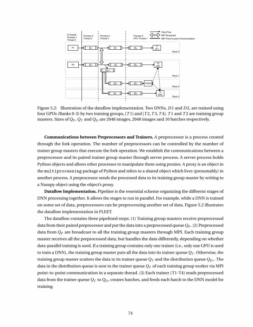
Rank 3

Rank 2

Rank 1

Rank 0P1

P2

QP QT

QP QT

QD

QD

QT QD

QT

QD

∗QD

T1 (D1)

T2 (D2)

T3(D2)

T4 (D2)

Process 0 CPU Thread 1

(if forked) Process 1 Thread 0

Process 0 Thread 0

Process 0 Thread 2

Data Flow MPI Broadcast MPI Point-to-point Communication

Figure 5.2: Illustration of the dataflow implementation. Two DNNs, D 1 and D 2, are trained usingfour GPUs (Ranks 0-3) by two training groups, (T 1) and (T 2, T 3, T 4). T 1 and T 2 are training groupmasters. Sizes of QP , QT and QD are 2048 images, 2048 images and 10 batches respectively.

Communications between Preprocessors and Trainers. A preprocessor is a process created

through the fork operation. The number of preprocessors can be controlled by the number of

trainer group masters that execute the fork operation. We establish the communications between a

preprocessor and its paired trainer group master through server process. A server process holds

Python objects and allows other processes to manipulate them using proxies. A proxy is an object in

the multiprocessing package of Python and refers to a shared object which lives (presumably) in

another process. A preprocessor sends the processed data to its training group master by writing to

a Numpy object using the object’s proxy.

Dataflow Implementation. Pipeline is the essential scheme organizing the different stages of

DNN processing together. It allows the stages to run in parallel. For example, while a DNN is trained

on some set of data, preprocessors can be preprocessing another set of data. Figure 5.2 illustrates

the dataflow implementation in FLEET.

The dataflow contains three pipelined steps: (1) Training group masters receive preprocessed

data from their paired preprocessor and put the data into a preprocessed queue QP . (2) Preprocessed

data from QP are broadcast to all the training group masters through MPI. Each training group

master receives all the preprocessed data, but handles the data differently, depending on whether

data-parallel training is used. If a training group contains only one trainer (i.e., only one GPU is used

to train a DNN), the training group master puts all the data into its trainer queue QT . Otherwise, the

training group master scatters the data to its trainer queue QT and the distribution queue QD ∗ . The

data in the distribution queue is sent to the trainer queue QT of each training group worker via MPI

point-to-point communication in a separate thread. (3) Each trainer (T1-T4) reads preprocessed

data from the trainer queue QT to QD , creates batches, and feeds each batch to the DNN model for

training.

74

Model Size

Trai

ning

Rat

e (#

GPU

=1)

Epoc

hs

0

50

100

150

200

0

5

10

15

20

25

250 500 750 1000

Training Rate Epochs

Figure 5.3: Correlations between model size of a DNN and the training rate and the number ofepochs until convergence.

5.5 Evaluations

We conduct a set of experiments to examine the efficacy of FLEET by answering the following

questions: (1) How much speedup can FLEET bring to ensemble training of heterogeneous DNNs?

(2) How do the pros and cons of the two paradigms in FLEET designs, local and global, play out in

handling the variations among DNNs? More specifically, does the greedy scheduling algorithm in

FLEET produce favorable schedules? How much waiting time does the round-by-round scheme in

FLEET cause, compared to eager scheduling schemes? (3) What is the overhead of runtime profiling,

scheduling, and checkpointing in FLEET?

We first describe the experiment settings (machines, baselines, etc.) in Section 5.5.1 and then

report our experiment results in Sections 5.5.2 and 5.5.3 to answer the questions.


5.5.1.1 DNNs

The DNNs used in this experiment are derived from DenseNets [Hua17] and ResNets [He16]. Both

models are the state-of-the-art network architectures that achieve high performance in various

learning tasks. We select these networks as the basis because, as structural DNNs, they are composed

of many Convolutional blocks, which have a standard interface making a block ready to be connected

with any other blocks. As a result, it is easy to derive new DNNs from them—one just needs to remove

or insert some Convolutional blocks.

We derive 100 experimental DNNs from six popular DNNs: DenseNet-121/169/201 and ResNet-

50/101/152. The first three are variations of DenseNets [Hua17]. The three variations share the same

75

structure, but differ in the number of DNN layers, indicated by their suffixes. The latter three are

variations of ResNets [He16].

The sizes of the DNN models vary from 232MB to 1.19GB. The distribution of their training

rates on a single GPU which vary from 21 to 176 images/sec. Different DNNs have different GPU

memory requirements and thus require different batch sizes to maximize GPU utilization. For

each, we use the maximum batch size that can fit into GPU’s memory. Figure 5.3 outlines the

relations between the training rates and model sizes of the DNNs, as well as the relations between

convergence rates (i.e., the number of epochs needed for the DNNs to converge) and their model

sizes. As model size increases, the training rate tends to drop as more computations are involved

in the DNN, but there are no clear correlations with the convergence rate. It is the reason that the

resource allocation algorithm in FLEET primarily considers training rate explicitly, and relies on the

periodical (re)scheduling to indirectly adapt to the variations of DNNs in the converging rates.

5.5.1.2 System

All experiments are conducted on SummitDev [Sum], a development machine for Summit super-

computer at Oak Ridge National Lab. Each node is equipped with two IBM POWER8 CPUs and

256GB DRAM, and four NVIDIA Tesla P100 GPUs. Each POWER8 CPU has 10 cores with 8 HW threads

each. The default SMT level is set to one unless noted otherwise. The number of cores allocated per

GPU is five in all the experiments. NVLink 1.0 is the connection among all GPUs and between CPUs

and GPUs within a node. EDR InfiniBand connects different nodes in a full fat-tree. The file system

is an IBM Spectrum Scale file system, which provides 2.5 TB/s for sequential I/O and 2.2 TB/s for

random I/O. Our experiments show that thanks to the large I/O throughput of the file system, I/O is

not the bottleneck of DNN training. The used CUDA version is 9.2.

FLEET is built on Tensorflow 1.12 (as the core training engine), Horovod v0.15.2 [Ser18] (as

the basis for distributed DNN training), and mpi4py v3.0.0 (for the pipeline construction). We set

inter_op_parallelism_threads and intra_op_parallelism_threads to # logical cores

for parallel TensorFlow operaitons on CPU. The used CUDA version is 9.2.

5.5.1.3 Profiling

To minimize the overhead of profiling, we only profile the training rates of each DNN in the ensemble

with the number of GPUs varying from one to Mt (Mt <M ), where Mt is determined based on the

training rates of each DNN on a single GPU. For profiling on m (m = 1, · · · , Mt ) GPUs, we train a

DNN for a maximum of 48 batches and use the training time of the last 20 batches to calculate the

exact training rate: ri (m ), i = 1, · · · , N . Based on the profiled training rates, we estimate the training

rates of each DNN when m >Mt .

Specifically, the profiling has three steps:

1. Collect the training rates of each DNN on a single GPU, R (1) = {ri (1)}, i = 1, · · · , N .

76

1 2 3 4 5 6 7 8Number of GPUs

0

200

400

600

800

1000

Trai

ning

Rat

e

Figure 5.4: The profiled training rates (images/sec) of 100 DNNs in an ensemble with Imagenet.

2. Estimate the number of GPUs required to make the DNN that has the smallest training rate

on a single GPU achieve the largest single-GPU training rate, Ma =�max(R (1))

min(R (1))

�

.

3. Collect the training rates of each DNN with the number of GPUs varying from two to Mt =

max(Ma , Mb ), where Mb = 2×G PU s P e r N o d e .

Note that steps 1 and 3 can be done in parallel because the trainings of different DNNs with

different number of GPUs are independent. The training rate of the i -th DNN with the number of

GPUs higher than Mt is estimated via the following equation:

ri (m ) =m ×ri (Mb )

Mb×� ri (Mb )

ri (Mb −1)×

Mb −1

Mb

�m−Mb. (5.5)

The formula for Mb and Equation 5.5 are the result of performance modeling on our observations

on the DNN performance trend as illustrated in Figure 5.4. It achieves a good tradeoff between the

profiling cost and the performance prediction accuracy.

The profiling process also measures the throughput of a range of preprocessors (#cores=1, 2, 4,

8, 16, 32) in the pipeline. This step is quick since preprocessing does not exhibit large variations.

Based on the profiled information, FLEET calculates the minimum number of preprocessors that

can meet the demands of an arbitrary M DNNs (with one running on one GPU), and uses it to set

the number of preprocessors.

5.5.1.4 Counterparts for Comparisons

• Baseline The baseline uses the default TensorFlow to train each DNN on one GPU indepen-

dently. Each DNN trainer has a preprocessor that preprocesses data for itself independently. A

GPU randomly picks one yet-to-be-trained DNN whenever it becomes free until there are no

DNN left.

• Homogeneous Training This is the state-of-the-art framework recently published [Pit18] for

ensemble DNN training. This framework allows the DNNs that get trained at the same time to

77

0

0.5

1

1.5

2

2.5

(20,100) (40,100) (60,100) (80,100) (100,100) (120,100) (140,100) (160,100)

Sp

ee

du

p

(#GPUs, #DNNs)

Homogeneous[24]FLEET-L

FLEET-G

Figure 5.5: The averaged speedups over the baseline in terms of the end-to-end time for training a100-DNN ensemble. The error bars show the variations.

share the preprocessed data. But it is designed for homogeneous DNN training, assuming no

variations among DNNs or the situation where the number of DNNs is no greater than the

number of GPUs. In our experiments, when there are more DNNs than GPUs, the framework

randomly picks a subset of the remaining DNNs to train, one DNN per GPU with shared

preprocessed data. After that subset is done, it picks another subset and repeats the process

until all DNNs are done.

• FLEET-G This is FLEET in the global paradigm.

• FLEET-L This is FLEET in the local paradigm as described in Section 5.3.3.3. Its difference

from FLEET-G is that as soon as a DNN is done, the released GPUs are immediately used to

train some remaining DNNs; which DNNs are picked is determined by the greedy algorithm

as in FLEET-G, but only locally (for the newly released GPUs) rather than globally.

5.5.2 End-to-End Speedups

Figure 5.5 reports the speedups of the three methods over the baseline method, in terms of the

end-to-end ensemble training time of the 100 DNNs. All runtime overhead for FLEET is included.

We repeat each measurement multiple times and report the average and error bars.

It shows the results in eight settings. The prior homogeneous framework shows large slowdowns

in the first four settings where the number of GPUs is less than the number of DNNs. The slowdowns

78

Wai

t tim

e/#G

PU in

sec

onds

5.0

10.0

50.0

100.0

20 GPU 100 DNN

40 GPU 100 DNN

60 GPU 100 DNN

80 GPU 100 DNN

100 GPU 100 DNN

120 GPU 100 DNN

140 GPU 100 DNN

160 GPU 100 DNN

Homogeneous[24] FLEET-L FLEET-G

Figure 5.6: Waiting time per GPU.

are due to the waiting of other GPUs for the slowest DNN to finish in each round, shown in Figure 5.6.

In the other four settings, the homogeneous framework performs similarly as the baseline does: As

there are more GPUs than DNNs, there is only one round, in which, the two methods use resource

similarly. The sharing of preprocessing in the homogeneous framework does not generate speedups

for these DNN trainings because the preprocessing is not the bottleneck for them.

FLEET-G gives the best overall performance, producing 1.12-1.92X speedups over the baseline.

The primary reason for the speedups come from its better resource allocation to the DNNs. The

bottom of Table 5.3 reports the mean and standard deviations of the running lengths of DNNs in

the first five flotillas in FLEET-G (80GPU,100DNN). In comparison to the data in the baseline and

FLEET-L (top rows in Table 5.3), the DNNs show much smaller variations in length, which indicate

the effectiveness of the GPU allocations in FLEET-G in evening out the differences among DNNs. At

the beginning, we thought that the catch to FLEET-G is the waiting time of some GPUs after they are

done with their work in a round. Our experiments, however, show the opposite effects. As Figure

5.6 shows, the average waiting time per GPU is smallest for FLEET-G. The reason is that the other

methods all suffer long waiting time at the end; because of their suboptimal resource allocation,

some GPUs have to work long after others to finish up the last few DNNs. FLEET-L gives notable but

fewer speedups for its less favorable decisions at resource allocation due to the local view.

Overall, FLEET gives larger speedups when #GPU > #DNN. It is worth noting that in such a

setting, there are still many flotillas to schedule and FLEET scheduler plays an important role.

The reason is that in many cases, the FLEET scheduler assigns multiple GPUs to one DNN. For

instance, 20 flotillas were created when training 100 DNN on 120 GPUs and 22 flotillas were created

when training 100 DNNs on 160 GPUs. When #GPU<#DNN, the speedups from FLEET are not that

significant but still substantial: 113–120% for three out of the four such settings in Figure 5.5.

79

Table 5.3: Mean and standard deviation of the running length of DNNs in seconds. (80 GPUs, 100DNNs)

Technique Flotilla ID Mean Std. Dev.

Baseline - 10372.2 4178.9FLEET-L - 6213 3580.0

0 2067.9 54.71 335.6 48.42 2291.9 26.0

FLEET-G 3 415.5 51.94 1072.2 364.05 2322.3 216.0

Table 5.4: Scheduling and checkpointing overhead.

(#GPU,#DNN)

Total TrainingTime (in sec)

SchedulingOverhead

CheckpointingOverhead

in sec in % in sec in %(20,100) 55200.1 20.1 0.037 1496.0 2.7(40,100) 30204.8 15.8 0.054 1156.0 3.8(60,100) 24495.0 14.0 0.060 986.0 4.0(80,100) 21891.0 12.0 0.057 816.0 3.7(100,100) 18359.1 10.1 0.058 782.0 4.3(120,100) 15323.9 9.9 0.068 680.0 4.4(140,100) 13366.3 9.3 0.073 680.0 5.1(160,100) 11825.2 10.2 0.092 748.0 6.3

5.5.3 Overhead

Table 5.4 reports the breakdown of the runtime overhead of FLEET-G. The overhead of scheduling

and checkpointing is at most 0.1% and 6.3% of the end-to-end training time in all the settings. Recall

that, due to wall-clock-time limitation of SummitDev, we have used the small Caltech256 dataset.

For large datasets (e.g., ImageNet), the overhead would become negligible. The profiling overhead

is independent of dataset size and solely depends on ensemble size. Recall that, profiling needs

the DNN to train for only a few steps in parallel. Its overhead is marginal for typical DNN trainings

on large datasets that take hours or days to train. On recent GPUs, a feature called Multi-Process

Services (MPS) could potentially allow multiple DNNs to be co-scheduled to a single GPU and

run concurrently. It is not considered in the current FLEET. To consider it, some co-run predictive

models could help, which could quickly predict the performance of a DNN when it co-runs with a

set of other DNNs on one GPU. The predictive performance can then be combined with the existing

performance models in FLEET to guide the scheduling of DNNs.

5.6 Related Work

Much research has been done to accelerate the training of a single DNN over distributed sys-

tems, such as Tensorflow from Google [Dea12; Aba15], Project Adams from Microsoft [Chi14], Fire-

Caffe [Ian16a], PipeDream [Har18], and GPipe [Hua18]. All those studies have focused on improving

the training speed of an individual DNN rather than ensemble training.

80

Recently, ensemble training starts drawing more attention. Besides the work by Pittman et

al. [Pit18], there are some other efforts [Gar18; Los16] on ensemble training, but they focus on

designing lightweight methods to form high-performing ensembles instead of improving pipeline

efficiency of ensemble training. HiveMind [Nar18] is a system designed for accelerating the training

of multiple DNNs on a single GPU by fusing common operations (e.g., preprocessing) across models.

It, however, lacks the essential support for distributed DNN training.

Another line of research that is relevant to this work is task scheduling on clusters or workflow

management systems. The scheduling of a set of tasks or workloads on clusters or multiproces-

sor systems has been extensively studied in the literature [Tur92; Shm95; Urg02; Aug11; Zah08;

Gra15; Cho16; Xu18; Ous13; Che16; Del14; Fei97]. Recent work including Gandiva [Xia18] and Tire-

sias [Gu19] design GPU cluster managers tailored for DNN workloads. They, however, lack the

flexibility supported in FLEET. First, they treat different jobs as independent black boxes. With-

out the MPI communication mechanisms we put into FLEET to enable flexible data exchanges of

TensorFlow-based workers and preprocessors, these schedulers cannot flexibly adjust the number of

workers for a DNN training. Second, as they treat the DNNs as separate jobs, they cannot support the

coordinations across DNNs in an ensemble, such as, the sharing of preprocessed data, cooperated

checkpointing at the appropriate times.

Load balancing techniques for parallel computers such as nearest neighbor assignment to

dynamically distribute workloads have been studied in [Kum94]. The way FLEET distributes DNN

training workloads are fundamentally different because an initial task assignment is not set at the

beginning but dynamically determined based on both the convergence status and the training rate

of each DNN.

HPC schedulers or workflow management systems schedule batch jobs on HPC systems. They

however cannot work directly with DNN ensembles. First, they treat different jobs as independent

black boxes. Without the MPI communication mechanisms we put into FLEET to enable flexible data

exchanges of TensorFlow-based workers and preprocessors, these schedulers cannot flexibly adjust

the number of workers for a DNN training. Second, as they treat the DNNs as separate jobs, they

cannot support the coordinations across DNNs in an ensemble, such as, the sharing of preprocessed

data, cooperated checkpointing at the appropriate times.

5.7 Conclusions

This chapter presented a systematic exploration on enabling flexible efficient ensemble training

for heterogeneous DNNs. It addressed two-fold challenges. First, it formalized the essence of the

problem into an optimal resource allocation problem, analyzes its computational complexity, and

presented an efficient greedy algorithm to effectively map DNNs to GPUs on the fly. Second, it

developed a set of techniques to seamlessly integrate distributed data-parallel training of DNN,

preprocessing sharing, and runtime DNN-to-GPU assignments together into a software framework,

FLEET. Experiments on 100 heterogeneous DNNs on SummitDev demonstrated that FLEET can

81

speed up the ensemble training by 1.12-1.92X over the default training method, and 1.23-1.97X over

the state-of-the-art framework that was designed for homogeneous ensemble training.

82

CHAPTER

6

IN-PLACE ZERO-SPACE MEMORY

PROTECTION FOR CNN

6.1 Introduction

As CNNs are increasingly explored for safety-critical applications such as autonomous vehicles and

aerospace, reliability of CNN inference is becoming an important concern. A key threat is memory

faults (e.g., bit flips in memory), which may result from environment perturbations, temperature

variations, voltage scaling, manufacturing defects, wear-out, and radiation-induced soft errors.

These faults change the stored data (e.g., CNN parameters), which may cause large deviations of

the inference results [Li17; Rea18; Rea16]. In this work, fault rate is defined as the ratio between the

number of bit flips experienced before correction is applied and the total number of bits.

Existing solutions have resorted to general memory fault protection mechanisms, such as Error

Correction Codes (ECC) hardware [Sri15], spatial redundancy, and radiation hardening [Yu10].

Being CNN-oblivious, these protections incur large costs. ECC, for instance, uses eight extra bits

in protecting 64-bit memory; spatial redundancy requires at least two copies of CNN parameters

to correct one error (called Triple Modular Redundancy (TMR) [Lyo62]); radiation hardening is

subject to substantial area overhead and hardware cost. The spatial, energy, and hardware costs

are especially concerning for safety-critical CNN inferences; as they often execute on resource-

constrained (mobile) devices, the costs worsen the limit on model size and capacity, and increase

the cost of the overall AI solution.

To address the fundamental tension between the needs for reliability and the needs for space/en-

ergy/cost efficiency, this work proposes the first zero space cost memory protection for CNNs. The

83

design capitalizes on the opportunities brought by the distinctive properties of CNNs. It further am-

plifies the opportunities by introducing a novel training scheme, Weight Distribution-Oriented Train-

ing (WOT), to regularize the weight distributions of CNNs such that they become more amenable

for zero-space protection. It then introduces a novel protection method, in-place zero-space ECC,

which removes all space cost of ECC protection while preserving protection guarantees.

Experiments on VGG16, ResNet-18, and SqueezeNet validate the effectiveness of the proposed

solution. Across all tested scenarios, the method provides protections consistently comparable

to those offered by existing hardware ECC logic, while removing all space costs. It hence offers a

promising replacement of existing protection schemes for CNNs.

6.2 Premises and Scopes

This work focuses on protections of 8-bit quantized CNN models. On the one hand, although the

optimal bit width for a network depends on its weight distribution and might be lower than 8, we

have observed that 8-bit quantization is a prevalent, robust, and general choice to reduce model

size and latency while preserving accuracy. In our experiments, both activations and weights are

quantized to 8-bit. Existing libraries that support quantized CNNs (e.g. NVIDIA TensorRT [Mig17],

Intel MKL-DNN [Mkl], Google’s GEMMLOWP [Jac17], Facebook’s QNNPACK [Qnn]) mainly target for

fast operators using 8-bit instead of lower bit width. On the other hand, previous studies [Li17; Rea18]

have suggested that CNNs should use data types that provide just-enough numeric value range and

precision to increase its fault tolerance. Our explorations on using higher precision including float32

for representing CNN parameters also show that 8-bit quantized models are the most resilient to

memory faults.

The quantization algorithm we used is symmetric range-based linear quantization that is well-

supported by major CNN frameworks (e.g. Tensorflow [Jac18], Pytorch [Zmo18]). Specifically, let

X be a floating-point tensor and X q be the 8-bit quantized version. X can be either weights or

activations from a CNN. The quantization is based on the following formula:

X q = r o und (X2n−1−1

max{|X |}), (6.1)

where n is the number of bits used for quantization. In our case, n = 8. The number of bits used for

accumulation is 32. Biases, if exist, are quantized to 32 bit integer.

Our work protects only weights for two reasons. Firstly, weights are usually kept in the mem-

ory. The longer they are kept, the higher the number of bit flips they will suffer from. This easily

results in a high fault rate (e.g. 1e-3) for weights. Activations, however, are useful only during an

inference process. Given the slight chance of having a bit flip during an inference process (usually

in milliseconds), protecting activations is not as pressing as protecting weights. Secondly, previous

work [Rea18] has shown that activations are much less sensitive to faults compared with weights.

84

Table 6.1: Accuracy and weight distribution of 8-bit quantized CNN models on ImageNet. Thepercentage rows use absolute values.

Model AlexNet VGG16 VGG16_bn Inception-V3 ResNet-18 ResNet-34 ResNet-50 ResNet-152 SqueezeNet#weights 61.1M 138.4M 138.4M 27.1M 11.7M 21.8M 25.5M 60.1M 1.2M

Accuracy(%)

Float32 56.52 71.59 73.36 69.54 69.76 73.31 76.13 78.31 58.09Int8 55.8 71.51 72.01 68.07 69.07 72.83 75.33 77.79 57.01

Percentage(%)

[0, 32) 95.09 97.69 98.83 97.98 99.66 99.76 99.65 99.49 95.16[32, 64) 4.88 2.27 1.16 1.96 0.32 0.23 0.34 0.49 4.62[64, 128] 0.03 0.04 0.01 0.06 0.02 0.01 0.01 0.01 0.22

1 2 3 4 5 6 7 8position

050

100150200250300350400

coun

t

Figure 6.1: Large weight (beyond [−64,63]) distributions in 8-byte (64-bit data) blocks forSqueezeNet on ImageNet. For instance, the first bar in (a) shows that of all the 8-byte data blocksstoring weights, around 380 have a large weight at the first byte.

Error Correction Codes (ECC) is commonly used in computer systems to correct memory faults.

They are usually described as (k , d , t ) code for length k code word, length d data, and t -bit error

correction. The number of required check bits is k −d .

6.3 In-Place Zero-Space ECC

Our proposed method, in-place zero-space ECC, builds on the following observation:Weights of a

well-trained CNN are mostly small values. The Percentage rows in Table 6.1 show the distributions

of the absolute values of weights in some popular 8-bit quantized CNN models. The absolute values

of more than 99% of the weights are less than 64. Even though eight bits are used to represent each

weight, if we already know that the absolute value of a weight is less than 64, the number of effective

bits to represent the value would be at most seven, and the remaining bit could be possibly used for

other purposes—such as error correction. We call it a non-informative bit.

The core idea of in-place zero-space ECC is to use non-informative bits in CNN parameters to

store error check bits. For example, the commonly used SEC-DED (64, 57, 1) code uses seven check

85

bits to protect 57 data bits for single error correction; they together form a 64-bit code word. If seven

out of eight consecutive weights are in range [−64,63], we can then have seven non-informative

bits, one per small weight. The essential idea of in-place ECC is to use these non-informative bits to

store the error check bits for the eight weights. By embedding the check bits into the data, it can

hence avoid all space cost.

For the in-place ECC to work, there cannot be more than one large weight in every 8 consecutive

weights. And the implementation has to record the locations of the large weights such that the

decoding step can find the error check bits from the data. It is, however, important to note that the

requirement of recording the locations of large weights would disappear if the large weights are

regularly distributed in data—an example is that the only place in which a large weight could appear

is the last byte of an 8-byte block. However, the distributions of large weights in CNNs are close to

uniform, as Figure 6.1 shows.

6.3.1 WOT

To eliminate the need of storing large weight locations in in-place ECC, we enhance our design

by introducing a new training scheme, namely weight-distribution oriented training (WOT). WOT

aims to regularize the spatial distribution of large weights such that large values can appear only at

specific places. We first formalize the WOT problem and then elaborate our regularized training

process.

Let Wl be the float32 parameters (including both weights and biases) in the l -th convolutional

layer and Wq

l be their values after quantization. Note that WOT applies to fully-connected layers as

well even though our discussion focuses on convolutional layers. WOT minimizes the sum of the

standard cross entropy loss ( f ({W ql }

Ll=1)) and weighted weight regularization loss (Frobenius norm

with the hyperparameter λ) subject to some weight distribution constraints on the weights:

min{W q

l }f ({W q

l }Ll=1) +λ

L∑

l=1

‖W ql ‖

2F , (6.2)

s .t . Wq

l ∈ Sl , l = 1, · · · , L . (6.3)

The weights are a four-dimensional tensor. If flattened, it is a vector of length Nl ×Cl ×Hl ×Wl ,

where Nl , Cl , Hl and Wl are respectively the number of filters, the number of channels in a filter, the

height of the filter, and the width of the filter, in the l -th convolutional layer. WOT adds constraints to

each 64-bit data block in the flattened weight vectors. Recall that, for in-place ECC to protect a 64-bit

data block, we need seven non-informative bits (i.e., seven small weights in the range [−64, 63]) to

store the seven check bits. To regularize the positions of large values in weights, the constraint on

the weights in the l -th convolutional layer can be given by Sl = {X | the first seven values in every

64-bit data block can have a value in only the range of [−64, 63]}.We next describe two potential solutions to the optimization problems.

86

6.3.1.1 ADMM-based Training

The above optimization problem can be formulated in the Alternating Direction Method of Multi-

pliers (ADMM) framework and solved in a way similar to an earlier work [Zha18c]. The optimization

problem (Eq. 6.2) is equivalent to:

min{W q

l }}f ({W q

l }Ll=1) +λ

L∑

l=1

‖W ql ‖

2F +

L∑

l=1

g l (Wq

l ), (6.4)

where g l (Wq

l ) =

0, if Wq

l ∈ Sl

+∞, otherwise.. Rewriting Eq. 6.4 in the ADMM framework leads to:

min{W q

l }f ({W q

l }Ll=1) +λ

L∑

l=1

‖W ql ‖

2F +

L∑

l=1

g l (Zl ), (6.5)

s .t . Wq

l = Zl , l = 1, · · · , L (6.6)

ADMM alternates between the optimization of model parameters ({W ql }

Ll=1 and the auxiliary

variables {Zl }Ll=1 by repeating the following three steps for k = 1, 2, · · · :

{W q ,k+1l }Ll=1 =arg min

{W ql }

Ll=1

f ({W ql }

Ll=1) +λ

L∑

l=1

‖W ql ‖

2F +γ

L∑

l=1

‖W ql −Zl +U k

l ‖2F , (6.7)

{Z k+1l }Ll=1 =arg min

{Zl }Ll=1

N∑

l=1

g l (Zl ) +L∑

l=1

λ

2‖W q ,k+1

l −Zl +U kl ‖

2F , (6.8)

U k+1l =U k

l +Wq ,k+1

l −Z k+1l . (6.9)

until the two conditions are met: ‖W q ,k+1l −Z k+1

l ‖2F ≤ ε and ‖Z k+1

l −Z kl ‖

2F ≤ ε.

Problem 6.7 can be solved using stochastic gradient descent (SGD) as the objective function is

differentiable. The optimal solution to the problem 6.8 is the projection of Wq ,k+1

l +U kl to set Sl . In

the implementation, we set a value in a 64-data block to 63 or -64 if the value is not in the eighth

position and is larger than 63 or smaller than -64.

Previous work has successfully applied the ADMM framework to CNN weight pruning [Zha18c]

and CNN weight quantization [Ren19] and shown remarkable compression results. But when it

is applied to our problem, experiments show that ADMM-based training cannot help reduce the

number of large values in the first seven positions of a 64-bit data block. Moreover, as the ADMM-

based training cannot guarantee that the constrain in Eq. 6.3 is satisfied, it is necessary to bound

the reamining large quantized values in the first 7 positions to 63 or -64 after the training, resulting

in large accuracy drops. Instead of ADMM-based training, WOT adopts an alternative approach

described below.

87

6.3.1.2 QAT with Throttling (QATT)

Our empirical explorations indicate that a simple quantization-aware training (QAT) procedure

combined with weight throttling can make the weights meet the constraint without jeopardising

the accuracy of a 8-bit quantized model. The training process iterates the following major steps for

each batch:

1. QAT: It involves forward-propagation using quantized parameters ({W ql }

Ll=1 and {b q

l }Ll=1) to

get the loss defined in Equation 6.2, back-propagation using quantized parameters, a update

step that applies float32 gradients to update float32 parameters ({Wl }Ll=1 and {bl }Ll=1), and a

quantization step that gets the new quantized parameters from their float32 version.

2. Throttling: It forces the quantized weights to meet the constraints defined in Eq. 6.3: If any

value in the first seven bytes of a 64-bit data block is larger than 63 (or less than -64), set the

value to 63 (or -64). The float32 versions are updated accordingly.

After the training, all of the values in the first seven positions of a 64-bit data block are ensured to

be within the range of [−64, 63], eliminating the need of storing large value positions for the in-place

ECC. It is worth noting that with WOT, all tested CNNs converge without noticeable accuracy loss

compared to the 8-bit quantized versions as Section 6.4 shows.

6.3.2 Full Design of In-Place Zero-Space ECC

In this part, we provide the full design of in-place zero-space ECC. For a given CNN, it first applies

WOT to regularize the CNN. After that, it conducts in-place error check encoding. The encoding uses

the same encoding algorithm as the standard error-correction encoding methods do; the difference

lies only in where the error check bits are placed.

There are various error-correction encoding algorithms. In principle, our proposed in-place

ECC could be generalized to various codes; we focus our implementation on SEC-DED codes for its

popularity in existing hardware-based memory protections for CNN.

Our in-place ECC features the same protection guarantees as the popular SEC-DED (72,64,1)

code but at zero-space cost. The in-place ECC uses the SEC-DED (64, 57, 1) code instead of (72, 64, 1)

to protect a 64-bit data block with the same protection strength. It distributes the seven error check

bits into the non-informative bits in the first seven weights.

As the ECC check bits are stored in-place, a minor extension to the existing ECC hardware is

required to support ECC decoding. As shown in Figure 6.2, the in-place ECC check bits and data

bits are swizzled to the right inputs to the standard ECC logic. The output of the ECC logic is then

used to recover the original weights: for each small weight (first seven bytes in a 8-byte data block),

simply copy the sign bit to its non-informative bit. As only additional wiring is needed to implement

this copy operation, no latency overhead is incurred to the standard ECC logic.

88

S W W W W W W

(Existing) ECC Logic with (64, 57) SEC-DED Hamming Code

P0

P0 P1…

…

… P6

S W W W W W WP6 S W W W W W WW

S W W W W WW S W W W W WW S W W W W W WW

7 check bits

8-weight (64-bit) block

57 data bits

S W W W W W WW … S W W W W W WW S W W W W W WW

8-weight (64-bit) block

Figure 6.2: Hardware design for in-place zero-space ECC protection.

6.4 Evaluations

We conducted a set of experiments to examine the efficacy of the proposed techniques in fault

protection and overhead. We first describe our experiment settings in Section 6.4.1 and then report

the effects of WOT and the proposed fault protection technique in Sections 6.4.2 and 6.4.3.


6.4.1.1 Models, Datasets, and Machines

The models we used in the fault injection experiments include VGG16 [Sim14], ResNet-18 [He16],

and SqueezeNet [Ian16b]. We choose these CNN models as representatives because: 1) VGG is a

typical CNN with stacked convolutional layers and widely used in transfer learning because of its

robustness. 2) ResNets are representatives of CNNs with modular structure (e.g. Residual Module)

and are widely used in advanced computer vision tasks such as object detection. 3) SqueezeNet

has much fewer parameters and represents CNNs that are designed for mobile applications. The

accuracies of these models are listed in Table 6.1. By default, We use the ImageNet dataset [Den09]

(ILSVRC 2012) for model training and evaluation. All the experiments are performed with PyTorch

1.0.1 on machines equipped with a 40-core 2.2GHz Intel Xeon Silver 4114 processor, 128GB of RAM,

and an NVIDIA TITAN Xp GPU with 12GB memory. Distiller [Zmo18] is used for 8-bit quantization.

The CUDA version is 10.1.

6.4.1.2 Counterparts for Comparisons

We compare our method (denoted as in-place) with the following three counterparts:

• No Protection (faulty): The CNN has no memory protection.

89

• Parity Zero (zero): It adds one parity bit to detect single bit errors in an eight-bit data block

(e.g. a single weight parameter). Once errors are detected, the weight is set to zero1.

• SEC-DED (ecc) It is the traditional SEC-DED [72,64,1] code-based protection in computer

systems [Sri15].

There are some previous proposals [Rea16; Azi18] of memory protections, which are however

designed for special CNN accelerators and provide without protection guarantees. The parity and

ECC represent the state of the art in the industry for memory protection that work generally across

processors and offer protection guarantees, hence the counterparts for our comparison.

6.4.2 WOT results

We evaluate the efficiency of WOT using the CNNs shown in Table 6.1. All the models are pre-trained

on ImageNet (downloaded from TorchVision2). We set λ to 0.0001 for all of the CNNs. Model training

uses stochastic gradient descent with a constant learning rate 0.0001 and momentum 0.9. Batch size

is 32 for VGG16_bn and ResNet-152, 64 for ResNet-50 and VGG16, and 128 for the remaining models.

Training stops as long as the model accuracy after weight throttling reaches its 8-bit quantized

version.

Figure 6.3 shows the changes of the total number of large values that are beyond [−64,63] in

the first seven positions of 8-byte blocks during the training on six of the CNNs. WOT successfully

reduces this number from more than 3,500–80,000 to near 0 for the models before throttling during

the training process. The remaining few large values in non-eighth positions are set to -64 or 63 at

the end of WOT. Note that VGG16_bn has around 10000 large values in the non eighth positions

after 8k iterations. Although more iterations further reduce this number, VGG16_bn can already

reach its original accuracy after weight throttling.

The accuracy curves of the models in the WOT training are shown in Figure 6.4. Overall, after

WOT training, the original accuracy of all the six networks are fully recovered. During the training,

the gap between the accuracy before throttling and after throttling is gradually reduced. For example,

the top-1 accuracy of SqueezeNet after 8-bit quantization is 57.01%. After the first iteration of WOT,

the accuracy before weight throttling is 31.38% and drops to 11.54% after throttling. WOT increases

the accuracy to 57.11% after 46k iterations with batch size 128 (around 4 epochs). All the other CNNs

are able to recover their original accuracy in only a few thousands of iterations. An exception is

VGG16, which reaches an accuracy of 71.50% (only 0.01% accuracy loss) after 20 epochs of training.

6.4.3 Fault injection results

In this set of experiments, we inject faults to CNN models and report the accuracy drops of CNN

models protected using different strategies. The fault model is random bit flip. Faults are injected to

1We have tried to set a detected faulty weight to the average of its neighbors but found it has worse performance thanParity Zero.

2https://pytorch.org/docs/master/torchvision/

90

https://pytorch.org/docs/master/torchvision/

Table 6.2: Accuracy drop of VGG16, ResNet-16, and SqueezeNet under different memory fault rates.

Model StrategyECC HW(Y/N)

SpaceOverhead (%)

Accuracy drop (%) under different fault rate1e-06 1e-05 1e-04 1e-03

VGG16

faulty N 0 0.31 ± 0.08 0.47 ± 0.09 1.35 ± 0.2 21.93 ± 5.7zero N 12.5 0.27 ± 0.05 0.36 ± 0.08 0.43 ± 0.13 1.04 ± 0.31ecc Y 12.5 0.0 ± 0.0 0.02 ± 0.02 0.35 ± 0.06 0.96 ± 0.14in-place Y 0 0.0 ± 0.0 0.02 ± 0.02 0.37 ± 0.07 0.93 ± 0.23

ResNet-18

faulty N 0 -0.09 ± 0.1 0.35 ± 0.23 4.35 ± 1.12 72.96 ± 1.48zero N 12.5 -0.06 ± 0.08 -0.08 ± 0.13 0.59 ± 0.3 4.35 ± 1.21ecc Y 12.5 0.0 ± 0.0 0.0 ± 0.01 -0.03 ± 0.08 2.8 ± 0.31in-place Y 0 0.0 ± 0.0 0.0 ± 0.01 -0.08 ± 0.09 2.96 ± 0.81

SqueezeNet

faulty N 0 0.12 ± 0.13 0.69 ± 0.31 9.39 ± 2.37 64.83 ± 0.5zero N 12.5 0.09 ± 0.12 0.11 ± 0.2 0.66 ± 0.29 8.16 ± 2.4ecc Y 12.5 0.0 ± 0.0 0.0 ± 0.0 0.12 ± 0.09 5.37 ± 0.66in-place Y 0 0.0 ± 0.0 0.0 ± 0.0 0.12 ± 0.09 5.19 ± 1.08

the weights of CNNs with memory fault rates varying from 10−9 to 0.001. The number of faulty bits

is the product of the number of bits used to represent weights of a CNN and the memory fault rate.

We repeated each fault injection experiment ten times.

Table 6.2 shows the mean accuracy drops with standard deviations under different memory fault

rates and the overheads introduced by the protection strategies for each model. Overall, the in-place

ECC protection and standard SEC-DED show similar accuracy drop patterns under various fault

rate settings as expected because they provide the same error correction capability, i.e., correcting a

single bit error and detecting double bit errors in a 64-bit data block. Both of the methods provide

stronger fault protection compared with the Parity Zero method. The space overhead is the ratio

between the extra number of bytes introduced by a protection strategy and the number of bytes

required to store weights. Parity Zero and SEC-DED encode 8-byte data with extra eight check bits

on average, making their space overhead 12.5%. In contrast, in-place ECC has zero space cost.

The fault injection experiments give the following insights on memory fault protection for CNNs.

First, larger models tend to suffer less from memory faults. For example, when fault rate is 0.0001

and no protection is applied, the accuracy drops of VGG16, ResNet-18, SqueezeNet (less than 2%,

8%, and 16% respectively) are increasing while the model size is decreasing (number of parameters

are 138M, 12M, and 1.2M respectively). Second, when the fault rate is small (e.g. less than 1e-05),

in-place ECC and standard SEC-DED can almost guarantee the same accuracy as the fault-free

model. Overall, the experiments confirm the potential of in-place zero-space ECC as an efficient

replacement of the standard ECC without compromising the protection quality.

6.5 Related Work

There are some early studies on fault tolerance of earlier neural networks (NN) [Pha95; Pro93; TH17];

they examined the performance degradation of NNs with various fault models on networks that

differ from modern CNNs in both network topologies and and model complexities.

Fault tolerance of deep neural networks (DNN) has recently drawn increasing attentions. Li et

al. [Li17] studied the soft error propagation in DNN accelerators and proposed to leverage symptom-

91

based error detectors for detecting errors and a hardware-based technique, selective latch hardening,

for detecting and correcting data-path faults. A recent work [Rea18; Are18] conducted some empirical

studies to quantify the fault tolerance of DNNs to memory faults and revealed that DNN fault

tolerance varies with respect to model, layer type, and structure. Zhang et al. [Zha18b] proposed

fault-aware pruning with retraining to mitigate the impact of permanent faults for systolic array-

based CNN accelerators (e.g., TPUs). They focused only on faults in the data-path and ignored

faults in the memory. Qin et al. [Qin17] studied the performance degradation of 16-bit quantized

CNNs under different bit flip rates and proposed to set values of detected erroneous weights as

zeros to mitigate the impact of faults. These prior works focused mainly on the characterization

of DNN’s fault tolerance with respect to various data types and network topologies. While several

software-based protection solutions were explored, they are preliminary. Some can only detect but

not correct errors (e.g. detecting extreme values [Li17]), others have limited protection capability

(e.g. setting faulty weights to zero [Qin17]).

Some prior work proposes designs of energy-efficient DNN accelerators by exploiting fault

tolerance of DNNs [Tem12; Kim18; Zha18a]. An accelerator design [Rea16] optimizes SRAM power

by reducing the supply voltage. It leverages active hardware fault detection coupled with bit masking

that shifts data towards zero to mitigate the impact of bit flips on DNNs’ model accuracy without

the need of re-training. Similar hardware faults detection techniques are later exploited in [Wha17;

Sal18; Zha18a; Hac19] to improve fault tolerance of DNNs. Azizimazreah et al. [Azi18] proposed

a novel memory cell designed to eliminate soft errors while achieving a low power consumption.

These designs are for some special accelerators rather than general DNN reliability protection. They

are still subject to various costs and offer no protection guarantees as existing ECC protections do.

This current work aims to reducing the space cost of protection to zero without compromising the

reliability of existing protections.

6.6 Future Directions

Besides 8-bit quantizations, there are proposals of even fewer-bit quantizations for CNN, in which,

there may be fewer non-informative bits in weight values. It is however worth noting that 8-bit

quantization is the de facto in most existing CNN frameworks; it has repeatedly shown in practice as

a robust choice that offers an excellent balance in model size and accuracy. Improving the reliability

of such models is hence essential. With that said, creating zero-space protections that works well

with other model quantizations is a direction worth future explorations.

A second direction worth exploring is to extend the in-place zero-space protection to other

error encoding methods (e.g., BCH [Cos83]). Some of them require more parity bits, for which, the

regularized training may need to be extended to create more free bits in data.

Finally, in-place zero-space ECC is in principle applicable to neural networks beyond CNN.

Empirically assessing the efficacy is left to future studies.

92

6.7 Conclusions

This chapter presented in-place zero-space ECC assisted with a new training scheme named WOT

to protect CNN memory. The protection scheme removes all space cost of ECC without compromis-

ing the reliability offered by ECC, opening new opportunities for enhancing the accuracy, energy

efficiency, reliability, and cost effectiveness of CNN-driven AI solutions.

93

0.0 0.5 1.0 1.5 2.0 2.5 3.0 3.5 4.0iterations(k)

05000

100001500020000250003000035000

coun

t

(a) AlexNet

0 1 2 3 4 5 6 7 8iterations(k)

1000020000300004000050000600007000080000

coun

t

(b) VGG16_bn

0.000.250.500.751.001.251.501.752.00iterations(k)

0

1000

2000

3000

4000

5000

coun

t

(c) ResNet-18

0 1 2 3 4 5 6 7 8iterations(k)

2000

4000

6000

8000

coun

t

(d) ResNet-34

0.0 2.5 5.0 7.5 10.012.515.017.520.0iterations(k)

0

2000

4000

6000

8000

10000

12000

coun

t

(e) ResNet-50

0 10 20 30 40iterations(k)

0500

100015002000250030003500

coun

t

(f) SqueezeNet

Figure 6.3: Changes of the total number of large values (beyond [−64, 63]) in the first 7 positions of8-byte (64-bit data) blocks before the throttling step during the WOT training process.

94

0.0 0.5 1.0 1.5 2.0 2.5 3.0 3.5 4.0iterations(k)

50515253545556

accu

racy

(%)

WOT: Before ThrottlingWOT: After ThrottlingOriginal Accuracy

(a) AlexNet

0 1 2 3 4 5 6 7 8iterations(k)

52.555.057.560.062.565.067.570.072.5

accu

racy

(%)


(b) VGG16_bn

0.000.250.500.751.001.251.501.752.00iterations(k)

60

62

64

66

68

accu

racy

(%)


(c) ResNet-18

0 1 2 3 4 5 6 7 8iterations(k)

64

66

68

70

72

accu

racy

(%)


(d) ResNet-34

0.0 2.5 5.0 7.5 10.012.515.017.520.0iterations(k)

55

60

65

70

75

accu

racy

(%)


(e) ResNet-50

0 10 20 30 40iterations(k)

10

20

30

40

50

accu

racy

(%)


(f) SqueezeNet

Figure 6.4: Accuracy curves before and after the throttling step during the WOT training process.

95

CHAPTER

7

CONCLUSIONS AND FUTURE WORK

Technical advances in machine learning (ML) have changed ML from a bespoke solution for special

tasks to a practical technology that can be deployed almost everywhere. This thesis focuses on

resolving challenges in adopting ML in real-world applications running on various systems. It

demonstrates the benefits of reuse-centric optimization for (1) efficient model discovery via reuse-

centric k-mean configuration in Chapter 3, composability-based fast CNN pruning in Chapter 4,

and ensemble training with data sharing in Chapter 5, and (2) reliable model inference via in-place

zero-space memory protection for CNN in Chapter 6. All of these optimizations share the common

reuse principle and the semantic-changing optimization philosophy. A high-level summary of the

thesis and research scope is shown in Figure 7.1.

Efficient Model Discovery. We start with k-means clustering and demonstrate implementation-

level reuse opportunities can be leveraged to accelerate k-means algorithm configuration by up

to 9X in Chapter 3. We then focus on efficient CNN model discovery, which is notoriously slow

and one of the major hurdles for shortening the time to market AI products. Chapter 4 presents a

compiler-based framework that speeds up CNN pruning by up to 186X via algorithm-level reuse.

We empirically uncover the existence of composability in the training of a collection of pruned CNN

models, design a compression-based algorithm to identify reuse opportunities, and propose a new

training scheme called composability-based CNN pruning to get benefits from reuse. Chapter 5

studies resource allocation problems when training a heterogeneous set of DNNs and presents a

flexible ensemble training framework called FLEET that achieves up to 2X speedup in ensemble

training. The framework integrates data-parallel distributed training, checkpointing, sharing of

preprocessed data, and efficient DNNs-to-GPUs mapping to best exploit infrastructure-level reuse

opportunities.

96

Semantic-PreservingOptimization in traditional

optimizing compilers

Reuse-CentricOptimization

Semantic-ChangingProgram Optimization

New Paradigm

K-Means Configuration (Chap. 3)

CNN Pruning (Chap. 4)

Ensemble Training (Chap. 5)

Memory Faults (Chap. 6)

Model Discovery

… …

Model Inference

… …

Figure 7.1: Summary of the thesis.

Reliable Model Inference. As CNNs are increasingly adopted in safety-critical applications,

making CNN a reliable solution becomes a matter of urgency. Chapter 6 presents in-place zero-

space ECC assisted with a new training scheme weight distribution-oriented training to improve

reliability of CNN inference. The new method provides the first known zero space cost memory

protection for CNNs without compromising the reliability offered by traditional ECC.

Future Work. This thesis has shed some light on how reuse opportunities can be leveraged to

ensure the efficiency and reliability of ML via innovations in both algorithms and programming

systems. Many fundamental questions on reuse-centric optimization remain for future exploration.

An immediate direction is on generalizing the success in efficient CNN pruning to a much

broader range of ML models (e.g. Recurrent Neural Networks), other search strategies (e.g., re-

inforcement learning and evolutionary algorithms), and other search objectives (e.g., accuracy).

The recent progress on neural architecture search (NAS) has shown some promising results on

automated model discovery. NAS helps eliminate the tedious and error-prone manual design ef-

forts. However, due to the lack of understanding of fundamental properties in trading off accuracy

for performance, it requires large-scale search which is too costly for many users. To reduce the

search cost, it is necessary to develop more efficient model search and training algorithms and then

automate them via novel programming system designs.

A more fundamental direction is to answer the many open questions lying at the foundation

level of reuse-centric optimization. What is the full taxonomy of reuse opportunities? Is it possible

to automatically uncover the hidden reuse opportunities in an arbitrary ML algorithm? Is there a

principled way to create and leverage reuse opportunities? How can we characterize the tradeoffs

between reuse benefits and the myriad other objectives (accuracy, size, energy, security, reliability,

interpretability, etc.) of ML? Are reuse-centric optimizations composable? How can we make them

work synergistically and avoid conflicts? What are the connections with other optimizations (in

97

both software and hardware) of deep learning? Answers to these questions will build the theoreti-

cal foundation for reuse-centric optimizations for deep learning. They will also pave the way for

generalizing the optimization to problems even beyond ML.

The achievements in improving CNN reliability elucidate the importance of a comprehensive

characterization of ML systems. Just as the small-weight observation motivates our in-place zero-

cost protection strategy, a comprehensive characterization of ML systems could expose more opti-

mization opportunities for improving system reliability and achieving the ultimate goal of making

AI dependable. The characterization should consider all layers from domain-specific requirements

(How much reliability is required? Is the application accuracy-critical or performance-critical?),

the choice of ML models (How robust is the model to adversarial attacks or faults?), and the relia-

bility of software stacks (Is the kernel implementation bug-free?) and computing hardware (Does

the hardware exhibit a relatively high fault rate?). The potential optimizations can go beyond the

reuse-centric approaches and requires the software-hardware co-design.

These explorations are just the beginning of the journey to the development of a new optimiza-

tion paradigm called semantic-changing program optimization, shown in Figure 7.1. Programming

systems work has long followed the contract that the program to be compiled and the program to

be executed should be equivalent. In other words, we conduct semantic-preserving optimization

for our programs. Now, with the wide adoption of ML in real applications, ML has become part

of our program and software. It is seemingly that ML has opened an opportunity to develop the

new optimization paradigm, semantic-changing program optimization. In this new paradigm, we

change the semantics or intentions of our program by optimizing our algorithms or workflows

instead of just instructions to obtain larger performance gain. And reuse-centric optimization is

only the tip of an iceberg. The new paradigm grows out of the principles in optimizing compiler. It

is inspired by the influence of approximate computing. As this thesis has shown, the new paradigm

has many potentials. And there are many open questions to answer: Are there principled ways to

characterize the nature of applicable situations? What is the set of techniques to develop to best

leverage these opportunities? What are the connections to modern programming language designs?

How to go beyond ML? What are the relations to other aspects of software (e.g., reliability, security)?

98

BIBLIOGRAPHY

[Aba15] Abadi, M. et al. TensorFlow: Large-Scale Machine Learning on Heterogeneous Systems.Software available from tensorflow.org. 2015.

[Agh17] Aghasi, A. et al. “Net-Trim: Convex Pruning of Deep Neural Networks with PerformanceGuarantee”. Advances in Neural Information Processing Systems. 2017, pp. 3180–3189.

[Ang13] Anguita, D. et al. “A Public Domain Dataset for Human Activity Recognition usingSmartphones.” ESANN. 2013.

[Are18] Arechiga, A. P. & Michaels, A. J. “The Effect of Weight Errors on Neural Networks”. 2018IEEE 8th Annual Computing and Communication Workshop and Conference (CCWC).IEEE. 2018.

[Art07] Arthur, D. & Vassilvitskii, S. “k-means++: The advantages of careful seeding”. Proceed-ings of the eighteenth annual ACM-SIAM symposium on Discrete algorithms. Societyfor Industrial and Applied Mathematics. 2007, pp. 1027–1035.

[Ash17] Ashok, A. et al. “N2N Learning: Network to Network Compression via Policy GradientReinforcement Learning”. arXiv preprint arXiv:1709.06030 (2017).

[Asu07] Asuncion, A. & Newman, D. UCI machine learning repository. 2007.

[Aug11] Augonnet, C. et al. “StarPU: a unified platform for task scheduling on heterogeneousmulticore architectures”. Concurrency and Computation: Practice and Experience 23.2(2011), pp. 187–198.

[Azi18] Azizimazreah, A. et al. “Tolerating Soft Errors in Deep Learning Accelerators with Reli-able On-Chip Memory Designs”. 2018 IEEE International Conference on Networking,Architecture and Storage (NAS). IEEE. 2018, pp. 1–10.

[Ba14] Ba, J. & Caruana, R. “Do deep nets really need to be deep?” Advances in neural informa-tion processing systems. 2014, pp. 2654–2662.

[Bal07] Balaprakash, P. et al. “Improvement strategies for the F-Race algorithm: Sampling designand iterative refinement”. International Workshop on Hybrid Metaheuristics. Springer.2007, pp. 108–122.

[Ber12] Bergstra, J. & Bengio, Y. “Random search for hyper-parameter optimization”. Journal ofMachine Learning Research 13.Feb (2012), pp. 281–305.

[Bir02] Birattari, M. et al. “A racing algorithm for configuring metaheuristics”. Proceedings of the4th Annual Conference on Genetic and Evolutionary Computation. Morgan KaufmannPublishers Inc. 2002, pp. 11–18.

[Bir10] Birattari, M. et al. “F-Race and iterated F-Race: An overview”. Experimental methods forthe analysis of optimization algorithms. Springer, 2010, pp. 311–336.

99

[Boj16] Bojarski, M. et al. “End to end learning for self-driving cars”. preprint arXiv:1604.07316(2016).

[Bot10] Bottou, L. “Large-scale machine learning with stochastic gradient descent”. Proceedingsof COMPSTAT’2010. Springer, 2010, pp. 177–186.

[Buc06] Bucilua, C. et al. “Model compression”. Proceedings of the 12th ACM SIGKDD inter-national conference on Knowledge discovery and data mining. ACM. 2006, pp. 535–541.

[Buc18] Buckler, M. et al. “EVA2: Exploiting Temporal Redundancy in Live Computer Vision”.arXiv preprint arXiv:1803.06312 (2018).

[Caf] Caffe Solver Prototxt.https://github.com/BVLC/caffe/wiki/Solver-Prototxt.

[Can16] Canziani, A. et al. “An analysis of deep neural network models for practical applications”.arXiv preprint arXiv:1605.07678 (2016).

[Che18a] Chen, H. et al. “The rise of deep learning in drug discovery”. Drug discovery today 23.6(2018), pp. 1241–1250.

[Che18b] Chen, T. et al. “{TVM}: An automated end-to-end optimizing compiler for deep learning”.13th {USENIX} Symposium on Operating Systems Design and Implementation ({OSDI}18). 2018, pp. 578–594.

[Che16] Cheng, D. et al. “Improving performance of heterogeneous mapreduce clusters withadaptive task tuning”. IEEE Transactions on Parallel and Distributed Systems 28.3 (2016),pp. 774–786.

[Chi14] Chilimbi, T. et al. “Project adam: Building an efficient and scalable deep learning trainingsystem”. 11th {USENIX} Symposium on Operating Systems Design and Implementation(OSDI). 2014, pp. 571–582.

[Chi01] Chilimbi, T. M. “Efficient representations and abstractions for quantifying and exploitingdata reference locality”. ACM SIGPLAN Notices. Vol. 36. 5. ACM. 2001, pp. 191–202.

[Chi02] Chilimbi, T. M. & Hirzel, M. “Dynamic hot data stream prefetching for general-purposeprograms”. ACM SIGPLAN Notices. Vol. 37. 5. ACM. 2002, pp. 199–209.

[Cho15] Chollet, F. et al. Keras. https://keras.io. 2015.

[Cho16] Chowdhury, M. et al. “{HUG}: Multi-Resource Fairness for Correlated and Elastic De-mands”. 13th {USENIX} Symposium on Networked Systems Design and Implementation({NSDI} 16). 2016, pp. 407–424.

[Coa12] Coates, A. & Ng, A. Y. “Learning feature representations with k-means”. Neural networks:Tricks of the trade. Springer, 2012, pp. 561–580.

[Cos83] Costello, D. J. Error Control Coding: Fundamentals and Applications. prentice Hall, 1983.

100

https://github.com/BVLC/caffe/wiki/Solver-Prototxt

https://keras.io

[Dav79] Davies, D. L. & Bouldin, D. W. “A cluster separation measure”. IEEE transactions onpattern analysis and machine intelligence 2 (1979), pp. 224–227.

[Dea12] Dean, J. et al. “Large scale distributed deep networks”. Advances in neural informationprocessing systems. 2012, pp. 1223–1231.

[Del14] Delimitrou, C. & Kozyrakis, C. “Quasar: resource-efficient and QoS-aware cluster man-agement”. ACM SIGARCH Computer Architecture News. Vol. 42. 1. ACM. 2014, pp. 127–144.

[Den09] Deng, J. et al. “Imagenet: A large-scale hierarchical image database”. 2009 IEEE confer-ence on computer vision and pattern recognition. Ieee. 2009, pp. 248–255.

[Dev18] Devlin, J. et al. “Bert: Pre-training of deep bidirectional transformers for language un-derstanding”. arXiv preprint arXiv:1810.04805 (2018).

[Din15a] Ding, Y. et al. “Top: A framework for enabling algorithmic optimizations for distance-related problems”. Proceedings of the VLDB Endowment 8.10 (2015), pp. 1046–1057.

[Din15b] Ding, Y. et al. “Yinyang k-means: A drop-in replacement of the classic k-means withconsistent speedup”. Proceedings of the 32nd International Conference on MachineLearning (ICML-15). 2015, pp. 579–587.

[Dra12] Drake, J. & Hamerly, G. “Accelerated k-means with adaptive distance bounds”. 5th NIPSworkshop on optimization for machine learning. 2012, pp. 42–53.

[Du89] Du, J. & Leung, J. Y.-T. “Complexity of scheduling parallel task systems”. SIAM Journalon Discrete Mathematics 2.4 (1989), pp. 473–487.

[Dun74] Dunn, J. C. “Well-separated clusters and optimal fuzzy partitions”. Journal of cybernetics4.1 (1974), pp. 95–104.

[Eck18] Eckert, C. et al. “Neural Cache: Bit-Serial In-Cache Acceleration of Deep Neural Net-works”. arXiv preprint arXiv:1805.03718 (2018).

[Elk03] Elkan, C. “Using the triangle inequality to accelerate k-means”. ICML. Vol. 3. 2003,pp. 147–153.

[Fei97] Feitelson, D. G. et al. “Theory and practice in parallel job scheduling”. Workshop on JobScheduling Strategies for Parallel Processing. Springer. 1997, pp. 1–34.

[Fig17] Figurnov, M. et al. “Spatially adaptive computation time for residual networks”. arXivpreprint (2017).

[Fow18] Fowers, J. et al. A Configurable Cloud-Scale DNN Processor for Real-Time AI. IEEE, 2018.

[Fri01] Friedman, J. et al. The elements of statistical learning. Vol. 1. Springer series in statisticsSpringer, Berlin, 2001.

101

[Fu17] Fu, J. et al. “Look closer to see better: Recurrent attention convolutional neural networkfor fine-grained image recognition”. Conf. on Computer Vision and Pattern Recognition.2017.

[Gar18] Garipov, T. et al. “Loss surfaces, mode connectivity, and fast ensembling of dnns”. Ad-vances in Neural Information Processing Systems. 2018, pp. 8789–8798.

[Gor18] Gordon, A. et al. “Morphnet: Fast & simple resource-constrained structure learning ofdeep networks”. IEEE Conference on Computer Vision and Pattern Recognition (CVPR).2018.

[Gra15] Grandl, R. et al. “Multi-resource packing for cluster schedulers”. ACM SIGCOMM Com-puter Communication Review 44.4 (2015), pp. 455–466.

[Gu19] Gu, J. et al. “Tiresias: A {GPU} cluster manager for distributed deep learning”. 16th{USENIX} Symposium on Networked Systems Design and Implementation ({NSDI} 19).2019, pp. 485–500.

[Hac19] Hacene, G. B. et al. “Training Modern Deep Neural Networks for Memory-Fault Robust-ness” (2019).

[Ham10] Hamerly, G. “Making k-means even faster”. Proceedings of the 2010 SIAM internationalconference on data mining. SIAM. 2010, pp. 130–140.

[Han15a] Han, S. et al. “Deep compression: Compressing deep neural networks with pruning,trained quantization and huffman coding”. arXiv preprint arXiv:1510.00149 (2015).

[Han15b] Han, S. et al. “Learning both weights and connections for efficient neural network”.Advances in neural information processing systems. 2015, pp. 1135–1143.

[Har18] Harlap, A. et al. “Pipedream: Fast and efficient pipeline parallel dnn training”. arXivpreprint arXiv:1806.03377 (2018).

[He15] He, K. et al. “Delving deep into rectifiers: Surpassing human-level performance onimagenet classification”. Proceedings of the IEEE international conference on computervision. 2015, pp. 1026–1034.

[He16] He, K. et al. “Deep residual learning for image recognition”. Proceedings of the IEEEconference on computer vision and pattern recognition. 2016, pp. 770–778.

[He18] He, Y. & Han, S. “ADC: Automated Deep Compression and Acceleration with Reinforce-ment Learning”. arXiv preprint arXiv:1802.03494 (2018).

[He17] He, Y. et al. “Channel pruning for accelerating very deep neural networks”. InternationalConference on Computer Vision (ICCV). Vol. 2. 2017, p. 6.

[Hin15] Hinton, G. et al. “Distilling the knowledge in a neural network”. preprint arXiv:1503.02531(2015).

102

[Hoc95] Hochbaum, D. S. Approximation Algorithms for NP-Hard Problems. PWS PublishingCompany, 1995.

[Hol12] Holger H. Hoos. Automated Algorithm Configuration and Parameter Tuning. Vol. 3.(Edited by Y. Hamadi, E. Monfroy, and F. Saubion) Springer Berlin Heidelberg, 2012.

[Hoo11] Hoos, H. H. “Automated algorithm configuration and parameter tuning”. Autonomoussearch. Springer, 2011, pp. 37–71.

[Hoo04] Hoos, H. H. & Stützle, T. Stochastic local search: Foundations and applications. Elsevier,2004.

[How17] Howard, A. G. et al. “Mobilenets: Efficient convolutional neural networks for mobilevision applications”. arXiv preprint arXiv:1704.04861 (2017).

[Hu16] Hu, H. et al. “Network trimming: A data-driven neuron pruning approach towardsefficient deep architectures”. arXiv preprint arXiv:1607.03250 (2016).

[Hua17] Huang, G. et al. “Densely connected convolutional networks”. Proceedings of the IEEEconference on computer vision and pattern recognition. 2017, pp. 4700–4708.

[Hua18] Huang, Y. et al. “Gpipe: Efficient training of giant neural networks using pipeline paral-lelism”. arXiv preprint arXiv:1811.06965 (2018).

[Hue16] Huerta, R. et al. “Online decorrelation of humidity and temperature in chemical sensorsfor continuous monitoring”. Chemometrics and Intelligent Laboratory Systems 157(2016), pp. 169–176.

[Hut07] Hutter, F. et al. “Automatic algorithm configuration based on local search”. AAAI. Vol. 7.2007, pp. 1152–1157.

[Hut09] Hutter, F. et al. “An experimental investigation of model-based parameter optimisa-tion: SPO and beyond”. Proceedings of the 11th Annual conference on Genetic andevolutionary computation. ACM. 2009, pp. 271–278.

[Hut11] Hutter, F. et al. “Sequential model-based optimization for general algorithm configu-ration”. International Conference on Learning and Intelligent Optimization. Springer.2011, pp. 507–523.

[Ian16a] Iandola, F. N. et al. “Firecaffe: near-linear acceleration of deep neural network trainingon compute clusters”. Proceedings of the IEEE Conference on Computer Vision andPattern Recognition. 2016, pp. 2592–2600.

[Ian16b] Iandola, F. N. et al. “SqueezeNet: AlexNet-level accuracy with 50x fewer parameters and<0.5 MB model size”. arXiv preprint arXiv:1602.07360 (2016).

[Mkl] Intel(R) Math Kernel Library for Deep Neural Networks (Intel(R) MKL-DNN). https://intel.github.io/mkl-dnn/. Accessed: 2019-08-16.

103

https://intel.github.io/mkl-dnn/

https://intel.github.io/mkl-dnn/

[Iof15] Ioffe, S. & Szegedy, C. “Batch normalization: Accelerating deep network training byreducing internal covariate shift”. International conference on machine learning. 2015,pp. 448–456.

[Jac17] Jacob, B. et al. gemmlowp: a small self-contained low-precision GEMM library. 2017.

[Jac18] Jacob, B. et al. “Quantization and training of neural networks for efficient integer-arithmetic-only inference”. Proceedings of the IEEE Conference on Computer Visionand Pattern Recognition. 2018, pp. 2704–2713.

[Jia14] Jia, Y. et al. “Caffe: Convolutional Architecture for Fast Feature Embedding”. arXivpreprint arXiv:1408.5093 (2014).

[Kal12] Kalogeratos, A. & Likas, A. “Dip-means: an incremental clustering method for estimatingthe number of clusters”. Advances in neural information processing systems. 2012,pp. 2393–2401.

[Kan18] Kandasamy, K. et al. “Neural architecture search with bayesian optimisation and optimaltransport”. Advances in Neural Information Processing Systems. 2018, pp. 2016–2025.

[Kho11] Khosla, A. et al. “Novel dataset for fine-grained image categorization: Stanford dogs”.Proc. CVPR Workshop on Fine-Grained Visual Categorization (FGVC). Vol. 2. 2011, p. 1.

[Kim18] Kim, S. et al. “Energy-efficient neural network acceleration in the presence of bit-levelmemory errors”. IEEE Transactions on Circuits and Systems I: Regular Papers 99 (2018),pp. 1–14.

[Kim14] Kim, Y. “Convolutional neural networks for sentence classification”. arXiv preprintarXiv:1408.5882 (2014).

[Kra13] Krause, J. et al. “3d object representations for fine-grained categorization”. ComputerVision Workshops (ICCVW), 2013 IEEE International Conference on. IEEE. 2013, pp. 554–561.

[Kra16] Krause, J. et al. “The unreasonable effectiveness of noisy data for fine-grained recogni-tion”. European Conference on Computer Vision. Springer. 2016, pp. 301–320.

[Kri12] Krizhevsky, A. et al. “Imagenet classification with deep convolutional neural networks”.Advances in neural information processing systems. 2012, pp. 1097–1105.

[Kum94] Kumar, V. et al. “Scalable load balancing techniques for parallel computers”. Journal ofParallel and Distributed computing 22.1 (1994), pp. 60–79.

[Lar99] Larus, J. R. “Whole program paths”. ACM SIGPLAN Notices. Vol. 34. 5. ACM. 1999, pp. 259–269.

[Lau05] Lau, J. et al. “Motivation for variable length intervals and hierarchical phase behavior”.IEEE International Symposium on Performance Analysis of Systems and Software, 2005.ISPASS 2005. IEEE. 2005, pp. 135–146.

104

[Law03] Law, J. & Rothermel, G. “Whole program path-based dynamic impact analysis”. SoftwareEngineering, 2003. Proceedings. 25th International Conference on. IEEE. 2003, pp. 308–318.

[Law97] Lawrence, S. et al. “Face recognition: A convolutional neural-network approach”. IEEEtransactions on neural networks 8.1 (1997), pp. 98–113.

[LeC95] LeCun, Y. & Bengio, Y. “Convolutional networks for images, speech, and time series”.The handbook of brain theory and neural networks 3361.10 (1995), p. 1995.

[LeC90] LeCun, Y. et al. “Optimal brain damage”. Advances in neural information processingsystems. 1990, pp. 598–605.

[Li17] Li, G. et al. “Understanding error propagation in deep learning neural network (DNN)accelerators and applications”. Proceedings of the International Conference for HighPerformance Computing, Networking, Storage and Analysis. ACM. 2017, p. 8.

[Li16] Li, H. et al. “Pruning filters for efficient convnets”. arXiv preprint arXiv:1608.08710 (2016).

[Li19] Li, L. & Talwalkar, A. “Random search and reproducibility for neural architecture search”.arXiv preprint arXiv:1902.07638 (2019).

[Lin17] Lin, J. et al. “Runtime Neural Pruning”. Advances in Neural Information ProcessingSystems. 2017, pp. 2178–2188.

[Liu17a] Liu, J. et al. “Sparse Deep Transfer Learning for Convolutional Neural Network.” AAAI.2017, pp. 2245–2251.

[Liu17b] Liu, Z. et al. “Learning efficient convolutional networks through network slimming”.2017 IEEE International Conference on Computer Vision (ICCV). IEEE. 2017, pp. 2755–2763.

[LI10] López-Ibánez, M. et al. “Exploratory analysis of stochastic local search algorithms inbiobjective optimization”. Experimental methods for the analysis of optimization algo-rithms. Springer, 2010, pp. 209–222.

[Los16] Loshchilov, I. & Hutter, F. “Sgdr: Stochastic gradient descent with warm restarts”. arXivpreprint arXiv:1608.03983 (2016).

[Lu12] Lu, W. et al. “Efficient processing of k nearest neighbor joins using mapreduce”. Pro-ceedings of the VLDB Endowment 5.10 (2012), pp. 1016–1027.

[Luo17a] Luo, J.-H. et al. “ThiNet: A Filter Level Pruning Method for Deep Neural Network Com-pression”. arXiv preprint arXiv:1707.06342 (2017).

[Luo18] Luo, L. et al. “Parameter Hub: High Performance Parameter Servers for Efficient Dis-tributed Deep Neural Network Training”. arXiv preprint arXiv:1801.09805 (2018).

[Luo17b] Luo, T. et al. “Dadiannao: A neural network supercomputer”. IEEE Transactions onComputers 66.1 (2017), pp. 73–88.

105

[Lyo62] Lyons, R. E. & Vanderkulk, W. “The use of triple-modular redundancy to improve com-puter reliability”. IBM journal of research and development 6.2 (1962), pp. 200–209.

[Mat18] Mathuriya, A. et al. “CosmoFlow: using deep learning to learn the universe at scale”.SC18: International Conference for High Performance Computing, Networking, Storageand Analysis. IEEE. 2018, pp. 819–829.

[McG17] McGill, M. & Perona, P. “Deciding how to decide: Dynamic routing in artificial neuralnetworks”. arXiv preprint arXiv:1703.06217 (2017).

[Mig17] Migacz, S. “8-bit inference with tensorrt”. GPU technology conference. Vol. 2. 2017, p. 7.

[Mio18] Miotto, R. et al. “Deep learning for healthcare: review, opportunities and challenges”.Briefings in bioinformatics 19.6 (2018), pp. 1236–1246.

[Mol16] Molchanov, P. et al. “Pruning convolutional neural networks for resource efficient transferlearning”. arXiv preprint arXiv:1611.06440 (2016).

[Mos18] Moshovos, A. et al. “Value-Based Deep-Learning Acceleration”. IEEE Micro 38.1 (2018),pp. 41–55.

[Nar18] Narayanan, D. et al. “Accelerating deep learning workloads through efficient multi-model execution”. NIPS Workshop on Systems for Machine Learning (December 2018).2018.

[NM97] Nevill-Manning, C. G. & Witten, I. H. “Identifying hierarchical structure in sequences: Alinear-time algorithm”. J. Artif. Intell. Res.(JAIR) 7 (1997), pp. 67–82.

[Nil08] Nilsback, M.-E. & Zisserman, A. “Automated flower classification over a large number ofclasses”. Computer Vision, Graphics & Image Processing, 2008. ICVGIP’08. Sixth IndianConference on. IEEE. 2008, pp. 722–729.

[O’K18] O’Keeffe, S. & Villing, R. “Evaluating pruned object detection networks for real-timerobot vision”. Autonomous Robot Systems and Competitions (ICARSC), 2018 IEEEInternational Conference on. IEEE. 2018, pp. 91–96.

[Ous13] Ousterhout, K. et al. “Sparrow: distributed, low latency scheduling”. Proceedings of theTwenty-Fourth ACM Symposium on Operating Systems Principles. ACM. 2013, pp. 69–84.

[Ovt15] Ovtcharov, K. et al. “Accelerating deep convolutional neural networks using specializedhardware”. Microsoft Research Whitepaper 2.11 (2015).

[Pan10] Pan, S. J. & Yang, Q. “A survey on transfer learning”. IEEE Transactions on knowledgeand data engineering 22.10 (2010), pp. 1345–1359.

[Par18] Park, J. et al. “Deep learning inference in facebook data centers: Characterization, per-formance optimizations and hardware implications”. arXiv preprint arXiv:1811.09886(2018).

106

[Pas19] Paszke, A. et al. “PyTorch: An Imperative Style, High-Performance Deep Learning Li-brary”. Advances in Neural Information Processing Systems 32. Ed. by Wallach, H. et al.Curran Associates, Inc., 2019, pp. 8024–8035.

[Pat18] Patton, R. M. et al. “167-PFlops deep learning for electron microscopy: from learningphysics to atomic manipulation”. Proceedings of the International Conference for HighPerformance Computing, Networking, Storage, and Analysis. IEEE Press. 2018, p. 50.

[Pha95] Phatak, D. S. & Koren, I. “Complete and partial fault tolerance of feedforward neuralnets”. IEEE Transactions on Neural Networks 6.2 (1995), pp. 446–456.

[Pit18] Pittman, R. et al. “Exploring flexible communications for streamlining DNN ensembletraining pipelines”. SC18: International Conference for High Performance Computing,Networking, Storage and Analysis. IEEE. 2018, pp. 807–818.

[Pro93] Protzel, P. W. et al. “Performance and fault-tolerance of neural networks for optimization”.IEEE transactions on Neural Networks 4.4 (1993), pp. 600–614.

[Qin17] Qin, M. et al. “Robustness of neural networks against storage media errors”. arXivpreprint arXiv:1709.06173 (2017).

[Qnn] QNNPACK: Open source library for optimized mobile deep learning. https://code.fb.com/ml-applications/qnnpack/. Accessed: 2019-08-16.

[Rah17] Rahman, A. et al. “Programming challenges of chatbot: Current and future prospective”.2017 IEEE Region 10 Humanitarian Technology Conference (R10-HTC). IEEE. 2017,pp. 75–78.

[Rat12] Ratnaparkhi, A. A. & Pilli, E. “Networks”. 2016 International Conference on EmergingTrends in Communication Technologies (ETCT) (2012), pp. 1–6.

[Rea16] Reagen, B. et al. “Minerva: Enabling low-power, highly-accurate deep neural networkaccelerators”. 2016 ACM/IEEE 43rd Annual International Symposium on ComputerArchitecture (ISCA). IEEE. 2016, pp. 267–278.

[Rea18] Reagen, B. et al. “Ares: A framework for quantifying the resilience of deep neural net-works”. 2018 55th ACM/ESDA/IEEE Design Automation Conference (DAC). IEEE. 2018,pp. 1–6.

[Ren19] Ren, A. et al. “ADMM-NN: An Algorithm-Hardware Co-Design Framework of DNNsUsing Alternating Direction Methods of Multipliers”. Proceedings of the Twenty-FourthInternational Conference on Architectural Support for Programming Languages andOperating Systems. ACM. 2019, pp. 925–938.

[Ren15] Ren, S. et al. “Faster r-cnn: Towards real-time object detection with region proposalnetworks”. Advances in neural information processing systems. 2015, pp. 91–99.

[Rou87] Rousseeuw, P. J. “Silhouettes: a graphical aid to the interpretation and validation ofcluster analysis”. Journal of computational and applied mathematics 20 (1987), pp. 53–65.

107

https://code.fb.com/ml-applications/qnnpack/

https://code.fb.com/ml-applications/qnnpack/

[Rus15] Russakovsky, O. et al. “Imagenet large scale visual recognition challenge”. InternationalJournal of Computer Vision (IJCV) 115.3 (2015), pp. 211–252.

[SG16] S. Guadarrama, N. S. TensorFlow-Slim: a lightweight library for defining, training andevaluating complex models in TensorFlow. https://github.com/tensorflow/tensorflow/tree/master/tensorflow/contrib/slim. 2016.

[Sal18] Salami, B. et al. “On the Resilience of RTL NN Accelerators: Fault Characterization andMitigation”. 2018 30th International Symposium on Computer Architecture and HighPerformance Computing (SBAC-PAD). IEEE. 2018, pp. 322–329.

[Sal17] Salimans, T. et al. “Evolution strategies as a scalable alternative to reinforcement learn-ing”. arXiv preprint arXiv:1703.03864 (2017).

[Sat11] Satopaa, V. et al. “Finding a" kneedle" in a haystack: Detecting knee points in system be-havior”. Distributed Computing Systems Workshops (ICDCSW), 2011 31st InternationalConference on. IEEE. 2011, pp. 166–171.

[Sei16] Seide, F. & Agarwal, A. “CNTK: Microsoft’s open-source deep-learning toolkit”. Proceed-ings of the 22nd ACM SIGKDD International Conference on Knowledge Discovery andData Mining. 2016, pp. 2135–2135.

[Ser18] Sergeev, A. & Del Balso, M. “Horovod: fast and easy distributed deep learning in Tensor-Flow”. arXiv preprint arXiv:1802.05799 (2018).

[Sha18] Sharma, H. et al. “Bit Fusion: Bit-Level Dynamically Composable Architecture for Accel-erating Deep Neural Network”. 2018 ACM/IEEE 45th Annual International Symposiumon Computer Architecture (ISCA). IEEE. 2018.

[Shm95] Shmoys, D. B. et al. “Scheduling Parallel Machines On-line”. SIAM J. Comput. 24.6 (1995),pp. 1313–1331.

[Sil16] Silberman, N. & Guadarrama, S. TensorFlow-Slim image classification model library.https://github.com/tensorflow/models/tree/master/research/slim.2016.

[Sil17] Silver, D. et al. “Mastering the game of go without human knowledge”. Nature 550.7676(2017), pp. 354–359.

[Sim14] Simonyan, K. & Zisserman, A. “Very deep convolutional networks for large-scale imagerecognition”. arXiv preprint arXiv:1409.1556 (2014).

[Sno12] Snoek, J. et al. “Practical bayesian optimization of machine learning algorithms”. Ad-vances in neural information processing systems. 2012, pp. 2951–2959.

[Sri15] Sridharan, V. et al. “Memory errors in modern systems: The good, the bad, and the ugly”.ACM SIGPLAN Notices 50.4 (2015), pp. 297–310.

108

https://github.com/tensorflow/tensorflow/tree/master/tensorflow/contrib/slim

https://github.com/tensorflow/tensorflow/tree/master/tensorflow/contrib/slim

https://github.com/tensorflow/models/tree/master/research/slim

[Sum] Summit User Guide Oak Ridge Leadership Computing Facility. https://www.olcf.ornl.gov/for-users/system-user-guides/summitdev-quickstart-guide/.Accessed 3/3/2019. 2019.

[Sze17] Sze, V. et al. “Efficient processing of deep neural networks: A tutorial and survey”. Pro-ceedings of the IEEE 105.12 (2017), pp. 2295–2329.

[Sze15] Szegedy, C. et al. “Going deeper with convolutions”. Proceedings of the IEEE conferenceon computer vision and pattern recognition. 2015, pp. 1–9.

[Sze16] Szegedy, C. et al. “Rethinking the inception architecture for computer vision”. Pro-ceedings of the IEEE Conference on Computer Vision and Pattern Recognition. 2016,pp. 2818–2826.

[Tem12] Temam, O. “A defect-tolerant accelerator for emerging high-performance applications”.ACM SIGARCH Computer Architecture News. Vol. 40. 3. IEEE Computer Society. 2012,pp. 356–367.

[Tia17] Tian, Q. et al. “Deep lda-pruned nets for efficient facial gender classification”. ComputerVision and Pattern Recognition Workshops (CVPRW), 2017 IEEE Conference on. IEEE.2017, pp. 512–521.

[Tom14] Tompson, J. J. et al. “Joint training of a convolutional network and a graphical modelfor human pose estimation”. Advances in neural information processing systems. 2014,pp. 1799–1807.

[TH17] Torres-Huitzil, C. & Girau, B. “Fault and error tolerance in neural networks: A review”.IEEE Access 5 (2017), pp. 17322–17341.

[Tur92] Turek, J. et al. “Scheduling parallelizable tasks: Putting it all on the shelf”. ACM SIGMET-RICS Performance Evaluation Review. Vol. 20. 1. ACM. 1992, pp. 225–236.

[Urg02] Urgaonkar, B. et al. “Resource overbooking and application profiling in shared hostingplatforms”. ACM SIGOPS Operating Systems Review 36.SI (2002), pp. 239–254.

[Wal10] Walkinshaw, N. et al. “Using compression algorithms to support the comprehensionof program traces”. Proceedings of the Eighth International Workshop on DynamicAnalysis. ACM. 2010, pp. 8–13.

[Wan11] Wang, X. “A fast exact k-nearest neighbors algorithm for high dimensional search us-ing k-means clustering and triangle inequality”. Neural Networks (IJCNN), The 2011International Joint Conference on. IEEE. 2011, pp. 1293–1299.

[Wel10] Welinder, P. et al. “Caltech-UCSD birds 200” (2010).

[Wen16] Wen, W. et al. “Learning structured sparsity in deep neural networks”. Advances inNeural Information Processing Systems. 2016, pp. 2074–2082.

109

https://www.olcf.ornl.gov/for-users/system-user-guides/summitdev-quickstart-guide/

https://www.olcf.ornl.gov/for-users/system-user-guides/summitdev-quickstart-guide/

[Wha17] Whatmough, P. N. et al. “14.3 A 28nm SoC with a 1.2 GHz 568nJ/prediction sparse deep-neural-network engine with> 0.1 timing error rate tolerance for IoT applications”. 2017IEEE International Solid-State Circuits Conference (ISSCC). IEEE. 2017, pp. 242–243.

[Wu08] Wu, X. et al. “Top 10 algorithms in data mining”. Knowledge and information systems14.1 (2008), pp. 1–37.

[Xia18] Xiao, W. et al. “Gandiva: Introspective cluster scheduling for deep learning”. 13th USENIXSymposium on Operating Systems Design and Implementation (OSDI 18). 2018, pp. 595–610.

[Xu18] Xu, L. et al. “A heterogeneity-aware task scheduler for spark”. 2018 IEEE InternationalConference on Cluster Computing (CLUSTER). IEEE. 2018, pp. 245–256.

[Yan17] Yang, T.-J. et al. “Designing energy-efficient convolutional neural networks using energy-aware pruning”. IEEE Conference on Computer Vision and Pattern Recognition (CVPR).2017.

[Ye18] Ye, J. et al. “Rethinking the Smaller-Norm-Less-Informative Assumption in ChannelPruning of Convolution Layers”. arXiv preprint arXiv:1802.00124 (2018).

[Yeh09] Yeh, I.-C. & Lien, C.-h. “The comparisons of data mining techniques for the predictiveaccuracy of probability of default of credit card clients”. Expert Systems with Applications36.2 (2009), pp. 2473–2480.

[Yu10] Yu, F.-X. et al. “Overview of Radiation Hardening Techniques for IC Design”. InformationTechnology Journal 9.6 (2010), pp. 1068–1080.

[Yu17] Yu, J. et al. “Scalpel: Customizing dnn pruning to the underlying hardware parallelism”.ACM SIGARCH Computer Architecture News. Vol. 45. 2. ACM. 2017, pp. 548–560.

[Zag16] Zagoruyko, S. & Komodakis, N. “Wide residual networks”. arXiv preprint arXiv:1605.07146(2016).

[Zah08] Zaharia, M. et al. “Improving MapReduce performance in heterogeneous environments.”Osdi. Vol. 8. 4. 2008, p. 7.

[Zha18a] Zhang, J. et al. “Thundervolt: enabling aggressive voltage underscaling and timing er-ror resilience for energy efficient deep learning accelerators”. Proceedings of the 55thAnnual Design Automation Conference. ACM. 2018, p. 19.

[Zha18b] Zhang, J. J. et al. “Analyzing and mitigating the impact of permanent faults on a systolicarray based neural network accelerator”. 2018 IEEE 36th VLSI Test Symposium (VTS).IEEE. 2018, pp. 1–6.

[Zha18c] Zhang, T. et al. “A systematic dnn weight pruning framework using alternating directionmethod of multipliers”. Proceedings of the European Conference on Computer Vision(ECCV). 2018, pp. 184–199.

110

[Zha18d] Zhang, T. et al. “Adam-admm: A unified, systematic framework of structured weightpruning for dnns”. arXiv preprint arXiv:1807.11091 (2018).

[Zha17] Zhao, B. et al. “Diversified visual attention networks for fine-grained object classifica-tion”. IEEE Transactions on Multimedia 19.6 (2017), pp. 1245–1256.

[Zha08] Zhao, Q. et al. “Knee point detection in BIC for detecting the number of clusters”. In-ternational Conference on Advanced Concepts for Intelligent Vision Systems. Springer.2008, pp. 664–673.

[Zho17] Zhong, R. Y. et al. “Intelligent manufacturing in the context of industry 4.0: a review”.Engineering 3.5 (2017), pp. 616–630.

[Zhu18] Zhu, H. et al. “TBD: Benchmarking and Analyzing Deep Neural Network Training”. arXivpreprint arXiv:1803.06905 (2018).

[Zmo18] Zmora, N. et al. Neural Network Distiller. https://doi.org/10.5281/zenodo.1297430. 2018.

[Zop16] Zoph, B. & Le, Q. V. “Neural architecture search with reinforcement learning”. arXivpreprint arXiv:1611.01578 (2016).

[Zop18] Zoph, B. et al. “Learning transferable architectures for scalable image recognition”.Proceedings of the IEEE conference on computer vision and pattern recognition. 2018,pp. 8697–8710.

111

reuse-centric programming system support of machine learning

Documents