retrieval of the diffuse attenuation coefficient(kd … · table 3-2 field measurements.....9 table...

RETRIEVAL OF THE DIFFUSE

ATTENUATION COEFFICIENT(Kd)

FROM SENTINEL 2 USING THE

2SEACOLOR MODEL AND Kd’S

IMPACTS ON SENSIBLE HEAT

FLUX OVER NAMTSO LAKE IN

TIBET, CHINA

PENG ZHANG

February 2018

SUPERVISORS:

Dr. Ir. Mhd, Suhyb Salama

Prof. Dr. Z, Su

ADVISOR:

Binbin, Wang

RETRIEVAL OF THE DIFFUSE

ATTENUATION COEFFICIENT

FROM SENTINEL 2 USING THE

2SEACOLOR MODEL AND Kd’S

IMPACTS ON SENSIBLE HEAT

FLUX OVER NAMTSO LAKE IN

TIBET, CHINA

PENG ZHANG

Enschede, The Netherlands, February 2018

Thesis submitted to the Faculty of Geo-Information Science and Earth Observation of the University of Twente in partial fulfilment of the requirements for the degree of Master of Science in Geo-Information Science and Earth Observation. Specialization: Water resources and Environment management

SUPERVISORS:

Dr. Ir. Mhd, Suhyb Salama

Prof. Dr. Z, Su

ADVISOR:

Binbin, Wang

THESIS ASSESSMENT BOARD:

Prof. Dr. Daphne. van der Wal (Chair)

Dr.Jaime Pitarch Portero (External examiner, NIOZ-TEXEL)

DISCLAIMER

This document describes work undertaken as part of a programme of study at Faculty of Geo-Information Science

and Earth Observation of the University of Twente. All views and opinions expressed therein remain the sole

responsibility of the author, and do not necessarily represent those of the Faculty.

ABSTRACT

Diffuse attenuation coefficient (Kd) for the underwater downwelling irradiance describes the attenuation of

incident light in a water column. Kd is a crucial indicator of the aquatic ecosystem quality and heating transfer

at the air-water interface. Here, an analytical forward model with an inversion scheme, 2SeaColor model,

was employed in combination with Sentinel 2 data to estimate Kd over Namtso Lake in Tibet Plateau, China.

Compared to existing models, 2SeaColor model can provide a stable solution for wide ranges of water types

in different depth. Kd map was produced by 2SeaColor model over Namtso Lake, and the spatial patterns

analysis of Kd map presents that the northeast and northwest of the lake showed higher Kd values and this

spatial distribution of Kd could attribute to the determination of the concentration of suspended particulate

matters, while the temporal distribution of Kd shared the similar pattern within the eight studied time series

from September to December of 2016 and 2017.

In addition, this study also focuses on the correlation between Kd and sensible heat flux. It is known that

Kd normally viewed as a constant in the mixed layer model or air-water interaction model. Physically,

however, an increase of Kd means more incident solar energy is capping in the water, thus, the Kd impacts

on water surface temperature, consequently on sensible heat flux. Therefore, this study firstly performed

the correlation analysis between Kd and lake surface temperature which is the MODIS L2 land surface

temperature products, and secondly conducted the correlation analysis between Kd and sensible heat flux.

The results of correlation analysis showed (1) it is not conclusive that the Kd is correlated to the lake surface

temperature in the temporal scale, while (2) most of the pixels in the Kd map and lake surface temperature

map present a high correlation coefficient and (3) the correlation coefficient for the Kd and sensible heat

flux is -0.85 which indicate that Kd is significantly negatively correlated to sensible heat flux. This study is

anticipated that Kd will find function in air-water interaction and mixed layer depth variation.

Keywords: diffuse attenuation coefficient, 2SeaColor model, Namtso Lake, sensible heat flux, correlation

analysis

ACKNOWLEDGEMENTS

This work dedicated to my parents (Rongbao Zhang & Ruilan Yang) and my girlfriend.

I would like to extend my gratitude to my supervisor, Dr. Ir. Mhd. Suhyb Salama and Prof. Dr. Z. Su.

I would also like to thank Binbin Wang who collected the field data for me.

i

TABLE OF CONTENTS

1. Introduction ........................................................................................................................................................... 1

1.1. Problem definition ......................................................................................................................................................2 1.2. Research objectives .....................................................................................................................................................2 1.3. Research questions ......................................................................................................................................................2

2. Literature review ................................................................................................................................................... 3

2.1. Kd with respect to heat transfer at the water-atmosphere interface ...................................................................3 2.2. Algorithms for estimation Kd ....................................................................................................................................3 2.3. Light propagation in Namtso Lake ..........................................................................................................................6 2.4. Sensible heat flux (H) ..................................................................................................................................................6

3. Study area and datasets ........................................................................................................................................ 7

3.1. Study area ......................................................................................................................................................................7 3.2. Datasets .........................................................................................................................................................................8

4. Methodology ....................................................................................................................................................... 12

4.1. Flowchart of methodology ..................................................................................................................................... 12 4.2. Models description ................................................................................................................................................... 13 4.3. Atmospheric correction (AC) for Sentinel 2 data ............................................................................................... 17 4.4. Data analysis and accuracy assessment ................................................................................................................. 18 4.5. Verification by Case 2 Regional Coast Colour (C2RCC) algorithm ................................................................ 18 4.6. The correlation analysis for Kd and H .................................................................................................................. 18

5. Results .................................................................................................................................................................. 21

5.1. Remote sensing reflectance and Kd from in-situ measurement ....................................................................... 21 5.2. Validation for Kd retrieved by 2SeaColor model ................................................................................................ 22 5.3. Estimating Kd from Sentinel 2 image ................................................................................................................... 23 5.4. Verification ................................................................................................................................................................ 26 5.5. Kd and sensible heat flux (H) ................................................................................................................................. 27

6. Discussion ........................................................................................................................................................... 29

6.1. Assessment of 2SeaColor model ........................................................................................................................... 29 6.2. The spatial and temporal characteristics of Kd in Namtso Lake...................................................................... 29 6.3. The relationship between Kd and H ..................................................................................................................... 30 6.4. The limitations .......................................................................................................................................................... 32

7. Conclusions......................................................................................................................................................... 32

RETRIEVAL OF THE DIFFUSE ATTENTUATION COEFFICIENT(Kd) FROM SENTINEL 2 USING THE 2SEACOLOR MODEL AND Kd’S IMPACT ON SENSIBLE HEAT FLUX

OVER NAMTSO LAKE IN TIBET CHINA

ii

LIST OF FIGURES

Figure 2-1 Schematic of Kd impacts on H. ............................................................................................................... 3

Figure 2-2 Schematic diagram of retrieving the Kd using the remote sensing method (Su et al., 2011). ........ 4

Figure 2-3 Schematic of the retrieving the Kd form Rrs. ......................................................................................... 4

Figure 3-1 Study area: the Namtso Lake. Source: Digital Globe taken on 6th Mar 2015, ground resolution

is 0.46 meters. ................................................................................................................................................................. 8

Figure 4-1 The flowchart of this study. ................................................................................................................... 13

Figure 4-2 The scattering of a water molecule. ...................................................................................................... 14

Figure 4-3 The scattering for a suspended particle. ............................................................................................... 16

Figure 4-4 Inversion scheme of 2SeaColor model................................................................................................. 17

Figure 4-5 Schematic diagram of temporal correlation. ........................................................................................ 19

Figure 4-6 Schematic diagram of spatial correlation. ............................................................................................. 20

Figure 5-1 Field measurements of Rrs and Kd spectrum curves (black) with their mean (red) and standard

deviation (blue) values. ............................................................................................................................................... 21

Figure 5-2 Derived Kd (490nm) from 2SeaColor model against known Kd (490nm) from field

measurements. ............................................................................................................................................................. 22

Figure 5-3 Derived Kd (490nm) from 2SeaColor model against known Kd (490nm) from convolved field

measurements. ............................................................................................................................................................. 23

Figure 5-4 Assessment of AC algorithms with the convolved field measured Rrs data in 10m and 60m

spatial resolutions. ....................................................................................................................................................... 24

Figure 5-5 Kd (490nm) maps estimated by 2SeaColor model using atmospheric corrected S2 data for

Namtso Lake on eight days: (a) 18th Oct. 2016, (b) 28th Oct.2016, (c) 6th Dec.2016, (d) 16th Dec.2016, (e)

27th Sept.2017, (f) 17th Oct.2017, (g) 22nd Oct.2017, and (h) 1st Dec.2017. ....................................................... 25

Figure 5-6 The correlation coefficients between Kd and LST. ............................................................................ 27

Figure 5-7 The correlation coefficient (r) map for Kd and LST. ......................................................................... 28

iii

LIST OF TABLES

Table 2-1 Algorithm for Kd(490) retrieval. ................................................................................................................ 5

Table 3-1 Ice phenology of Namtso Lake during 2001-2010. Freeze Onset (FO) indicates first ice

formation; Freeze-Up (FU) refers to the date that the lake is fully covered by ice; Break-Up (BU) means

the date is appearing the detectable ice-free water; Water Clean Ice denotes the end of ablation date that

the full disappearance of ice. ........................................................................................................................................ 7

Table 3-2 Field measurements. .................................................................................................................................... 9

Table 3-3 The dates of used S2 MSI data. ................................................................................................................. 9

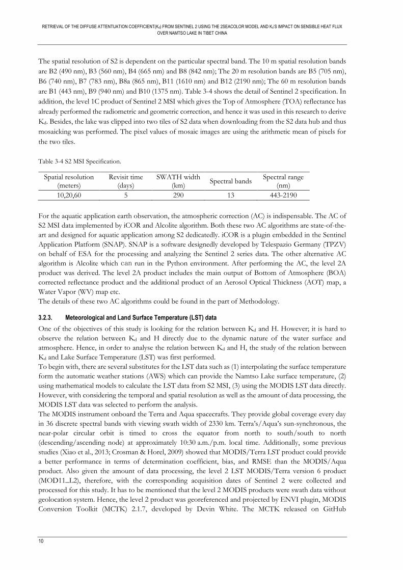
Table 3-4 S2 MSI Specification. ............................................................................................................................... 10

Table 4-1 The coefficients description in the attenuation process. .................................................................... 14

Table 5-1 The average values (mean) and standard deviations (STD) for the Rrs and Kd of selected

wavelengths over Namtso Lake. .............................................................................................................................. 21

Table 5-2 Statistical parameters of the iCOR and Alcolite AC algorithms in 10m and 60m spatial

resolutions. ................................................................................................................................................................... 24

Table 5-3 The statistic variables of Kd for C2RCC and 2SeaColor models on three days. DR represents

dynamic range (N=10). .............................................................................................................................................. 26

Table 5-4 The meteorological data, computed H and the correlation coefficients. ........................................ 28



iv

LIST OF ACRONYMS

Kd Diffuse attenuation coefficient

IOPs Inherent optical properties

H Sensible heat flux

G Heat storage in water

TP Tibet Plateau

AC Atmospheric correction

a Absorption coefficient

bb Backscattering coefficient

CZCS Atmospherically Correct Coastal Zone Colour Scanner

COASTLOOC Coastal Surveillance through Observation of Ocean Colour

GOCI Geostationary Ocean Colour Imager

Chl-a Chlorophyll-a

SPM Suspended particulate matters

PAR Photosynthetically Active Radiation

LST Lake surface temperature

S2 MSI Sentinel 2 MultiSpectral Instrument

MSTK MODIS Conversion Toolkit

U Wind speed

Ta Near surface temperature

Ts Lake surface temperature

Rrs Remote sensing reflectance

Ed Downwelling irradiance

Eu Upwelling irradiance

Lu Upwelling radiance

R Temporal correlation coefficient

r Spatial correlation coefficient



1

1. INTRODUCTION

Diffuse attenuation coefficient (Kd in m-1) for underwater downwelling irradiance is a key variable that can

quantify the attenuation processes of incident light in a water column. It is a bulk measurement of the light

propagation, and it could be used to evaluate heat and evaporation transfer at the water-atmosphere interface

on the one hand. On the other hand, Kd can determine whether there is sufficient Photosynthetically Active

Radiation (PAR:400-700 nm) that can support photosynthesis in a water column(Stramska & Zuzewicz,

2013; Loiselle et al., 2009; Wu, Tang, Sathyendranath, & Platt, 2007). PAR is fundamental for the aquatic

life activities. Thus, Kd is a vital indicator of inland water quality which is of significance to the function of

the aquatic ecosystem.

Due to the increasing anthropogenic activities and industry pollutions, a large number of inland waters are

deteriorating (Pu, Liu, Qu, & Sun, 2017; Vorosmarty et al., 2010). The traditional methods to quantify and

monitor the inland water quality are labour-intensive and time-consuming. Satellite remote sensing

compared to the conventional methods can provide an effective way to obtain the water status parameters

on spatial-scales (Glasgow, Burkholder, Reed, Lewitus, & Kleinman, 2004; Dekker, Vos, & Peters, 2002). It

can also provide synoptic views of the water target over large areas and extend the predictable time periods.

Remote sensing can measure the water leaving signals that characterize the optical properties of the water

body. The signals recorded by sensors can disintegrate into some sub-signals. These sub-signals stem from

the different attenuation processes in the atmosphere, at the water-atmosphere interface, and in the water

column. Water leaving reflectance (rho_w) is the signal of interest as it can be related to IOPs. To obtain

rho_w, atmospheric correction (AC) is needed to remove the interactions between the solar radiation and

atmosphere. Therefore, this research performs both atmosphere correction of the signals recorded by

sensors and using inversion scheme to quantify the inherent optical properties and then to derive the Kd.

From this perspective, with remote sensing technique, the interaction of transmitted solar radiation in a

water column with the water constituents can be detected and quantified through IOPs (Mobley, 1994).

These IOPs could be absorption and scattering caused by the optically significantly water components and

thus determine the Kd. Further, eutrophication and thermal stratification (Liu et al., 2016) often lead to an

increase of diffuse attenuation coefficient and water turbidity.

Since the operational algorithm (C2RCC) to retrieve Kd of Sentinel 2 released recently, therefore, in this

thesis, the MultiSpectral Instrument (MSI) on-board the Sentinel 2 satellite series designed by European

Space Agency (ESA) will be used for retrieved Kd by 2SeaColor model (Salama & Verhoef, 2015) and then

validated by corresponding in-situ data as well as verified by C2RCC.

It is studied that Kd affected the incident solar energy partitioning in the water column at different depth by

Read, Rose, Winslow, & Read, (2015). Thus, Kd could impact on the water surface temperature,

consequently on the heat transfer at the water-atmosphere boundary. Sensible heat flux (H) is one of the

important heat flux components in the heat transfer process. Because H is capable of computing by the

readily derived temperature. This thesis also analyses the relationship between Kd and sensible heat flux (H)

by firstly investigated the dependence of Kd on water surface temperature.

To sum up, the thesis produced the Kd map in varied time series using the 2SeaColor model in combination

with Sentinel 2 data attempting to derive the spatial and temporal variations of Namtso Lake in Tibet Plateau

(TP). Besides, this thesis also analysed the Kd impact on the water surface temperature and the sensible heat



2

flux to look for how Kd affect the H. It is expected to provide a robust exploration of the Kd impact on air-

water interaction.

1.1. Problem definition

Despite the crucial significance of Kd in the biogeochemical functioning of the inland water system; our

current knowledge is incapable of fully understanding the optical complexity of interaction between the light

and water components. In addition, most of the previous works developed the algorithms for the remote

retrieval of Kd through employing (quasi) single scattering approximation and they normally generate large

uncertainty (more than 45%) on derived IOPs to the overall errors over turbid water(Lee, Arnone, Hu,

Werdell, & Lubac, 2010a; Salama & Stein, 2009). Some were focused on improving atmospheric correction

to obtain a higher accuracy of water leaving reflectance and then deducting the errors of Kd, very little

research has been performed to improve the forward model for radiative transfer in water. However,

2SeaColor model developed by is a forward remote sensing model with an inversion scheme for turbid

water. 2SeaColor model will be used in this research to investigate the opportunities of Sentinel 2 MSI to

estimate Kd in turbid inland water such as Namtso Lake.

Besides, previous studies (Frankignoul, Czaja, & L’Heveder, 1998; Giardino, Pepe, Brivio, Ghezzi, & Zilioli,

2001; Zhang et al., 2015) specified the Kd of the visible part of radiation as a constant value when they are

applying the water-heat transfer models and sea surface temperature models and, thus, could result in an

inconsistency between model and observation (Denman, 1973). In fact, Kd is with large variations spatially

and temporally (Zheng et al., 2016; Tiwari & Shanmugam, 2014). Therefore, it is urged to investigate the

spatial and temporal variations of Kd and its relationship between water surface temperature as well as H

for the inland waters.

1.2. Research objectives

The main objective of this study is to derive diffuse attenuation coefficient (Kd) for Sentinel 2 data in Namtso

lake and to assess the related errors using in situ data.

The specific objectives are:

1. To apply 2SeaColor model to estimate Kd over Namtso Lake.

2. To validate and assess the 2SeaColor model for Sentinel 2.

3. To analyse the spatial and temporal characteristics of Kd in Namtso Lake. 4. To analyse the relationship between Kd and H regarding spatial and temporal variations in Namtso

Lake.

1.3. Research questions

The following questions need to be addressed to achieve the objectives mentioned above for this work:

1. Is 2SeaColor model applicable to the Sentinel 2 series satellites?

2. To what extent that the derived Kd map from Sentinel 2 is reliable and applicable?

3. What is the spatial and temporal characteristic of Kd in Namtso lake?

4. What is the relationship between Kd and H with respect to spatial and temporal variations?



3

2. LITERATURE REVIEW

2.1. Kd with respect to heat transfer at the water-atmosphere interface

The presence of water constituents leads to the increasing of Kd. An increasing Kd value could lead to a

reduction of the light penetration along the propagation path within the water column, thus, the temperature

of the upper layer of a water body will increase (Chen, Zhang, Xing, Ishizaka, & Yu, 2017). In other words,

Kd effects the incident light energy distribution regarding vertical heat transfer within the water. And it is

well known that one of the driven mechanism of sensible heat flux (H) is the gradient between surface

temperature and air temperature (Brutsaert, 1982), thus Kd plays a role in the heat transfer process at the

water-atmosphere interface (Wu, Platt, Tang, & Sathyendranath, 2008). Besides, other physical processes

can also influence water surface temperatures, for example, mixing driven by wind or convection (Read et

al., 2012), or inflows (Imberger & Patterson, 1980).

Due to the lack of vertical temperature profile data of the Namtso Lake, heat storage in the water body (G)

cannot computed. Thus, this thesis selected the sensible heat flux as the representative of heat transfer

progress at the water-atmosphere interface. In summary, Figure 2-1 shows the physical process that Kd

impact on H theoretically.

Some studies were carried out on the importance of Kd with respect to the heat transfer at the water-

atmosphere interface. Chang & Dickey (2004) suggested that increased Kd could lead to the greater heat

gain at the upper layer of the water body. The gained heat could result in the enhancement of the thermocline

and lagging of the Chl-a in the eutrophic depth. Wu et al. (2007) studied the bio-optical heating caused by

Kd increasing and its contribution to upper dynamics in the Labrador Sea. The impact of Kd on sea surface

temperature was investigated by Wu et al. (2007) through comparing the mixed layer model that employed

the modelled Kd and an assumed constant Kd. Their results showed the sea surface temperature increased

1 ℃ at most of the sea and up to 2.7 ℃ at the high Kd value area.

However, there are other factors also determine the H, for instance, air temperature, wind speed,

atmospheric stability (Wang, Ma, Ma, & Su, 2017) except for Kd. Hence, it is complicated to find the relation

between Kd and H.

Figure 2-1 Schematic of Kd impacts on H.

2.2. Algorithms for estimation Kd

Figure 2-2 explicated the sources of signals using the remote sensing method to retrieve the Kd for the

inland water system, i.e. water constituents, adjacent land pixels, and atmosphere. Obviously, in order to

derive Kd, atmospheric correction (AC) algorithm and Kd retrieval algorithm are indispensable. A reliable

AC algorithm was implemented to remove the atmospheric interaction and the adjacent effect. AC algorithm

is going to be elaborated in the following part. Apart from AC, the analytical Kd retrieval algorithms focus

on the signal inside of the water.



4

Figure 2-2 Schematic diagram of retrieving the Kd using the remote sensing method (Su et al., 2011).

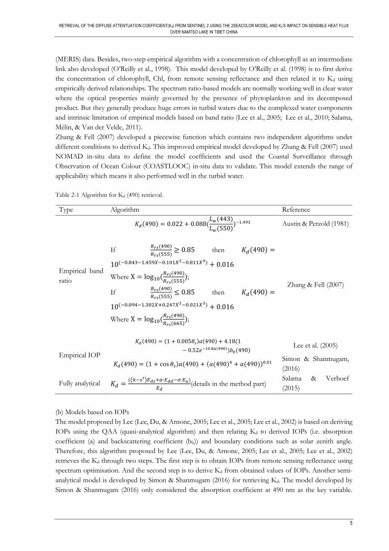
The models used for estimating Kd can be categorised into two types. The first ((a) in Figure 2-3) is the

empirical model which based on the band ratio. The second ((b) in Figure 2-3) is based on the derived IOPs

(i.e. absorption coefficient (a) and the backscattering coefficient (bb)). The relationship between Kd and IOP

could be “semi” analytical or empirical both. And the details are unfolded below.

(a)

(b)

Figure 2-3 Schematic of the retrieving the Kd form Rrs.

(a) Empirical models based on band ratio

Austin & Petzold (1981) developed an empirical algorithm to derive Kd (490) from Atmospherically Correct

Coastal Zone Colour Scanner (CZCS) data utilising the blue-green ratio of upwelling radiances above water

(Lw). All the algorithms discussed in this part showed in Table 2-1. A slightly modified approach was

proposed by Kratzer, Brockmann, & Moore (2008) to retrieve Kd (490) from Medium Imaging Spectrometer



5

(MERIS) data. Besides, two-step empirical algorithm with a concentration of chlorophyll as an intermediate

link also developed (O’Reilly et al., 1998). This model developed by O’Reilly et al. (1998) is to first derive

the concentration of chlorophyll, Chl, from remote sensing reflectance and then related it to Kd using

empirically derived relationships. The spectrum ratio-based models are normally working well in clear water

where the optical properties mainly governed by the presence of phytoplankton and its decomposed

product. But they generally produce huge errors in turbid waters due to the complexed water components

and intrinsic limitation of empirical models based on band ratio (Lee et al., 2005; Lee et al., 2010; Salama,

Mélin, & Van der Velde, 2011).

Zhang & Fell (2007) developed a piecewise function which contains two independent algorithms under

different conditions to derived Kd. This improved empirical model developed by Zhang & Fell (2007) used

NOMAD in-situ data to define the model coefficients and used the Coastal Surveillance through

Observation of Ocean Colour (COASTLOOC) in-situ data to validate. This model extends the range of

applicability which means it also performed well in the turbid water.

Table 2-1 Algorithm for Kd (490) retrieval.

Type Algorithm Reference

Empirical band

ratio

𝐾𝑑(490) = 0.022 + 0.088(𝐿𝑤(443)

𝐿𝑤(550))−1.491 Austin & Petzold (1981)

If 𝑅𝑟𝑠(490)

𝑅𝑟𝑠(555)≥ 0.85 then 𝐾𝑑(490) =

10(−0.843−1.459𝑋−0.101𝑋2−0.811𝑋3) + 0.016

Where X = log10(𝑅𝑟𝑠(490)

𝑅𝑟𝑠(555));

If 𝑅𝑟𝑠(490)

𝑅𝑟𝑠(555)≤ 0.85 then 𝐾𝑑(490) =

10(−0.094−1.302𝑋+0.247𝑋2−0.021𝑋3) + 0.016

Where X = log10(𝑅𝑟𝑠(490)

𝑅𝑟𝑠(665));

Zhang & Fell (2007)

Empirical IOP

𝐾𝑑(490) = (1 + 0.005𝜃𝑠)𝑎(490) + 4.18(1

− 0.52𝑒−10.8𝑎(490))𝑏𝑏(490) Lee et al. (2005)

𝐾𝑑(490) = (1 + cos 𝜃𝑠)𝑎(490) + (𝑎(490)4 + 𝑎(490))0.01 Simon & Shanmugam,

(2016)

Fully analytical 𝐾𝑑 =((𝑘−𝑠′)𝐸𝑑𝑠+𝛼∙𝐸𝑑𝑑−𝜎∙𝐸𝑢)

𝐸𝑑(details in the method part)

Salama & Verhoef

(2015)

(b) Models based on IOPs

The model proposed by Lee (Lee, Du, & Arnone, 2005; Lee et al., 2005; Lee et al., 2002) is based on deriving

IOPs using the QAA (quasi-analytical algorithm) and then relating Kd to derived IOPs (i.e. absorption

coefficient (a) and backscattering coefficient (bb)) and boundary conditions such as solar zenith angle.

Therefore, this algorithm proposed by Lee (Lee, Du, & Arnone, 2005; Lee et al., 2005; Lee et al., 2002)

retrieves the Kd through two steps. The first step is to obtain IOPs from remote sensing reflectance using

spectrum optimisation. And the second step is to derive Kd from obtained values of IOPs. Another semi-

analytical model is developed by Simon & Shanmugam (2016) for retrieving Kd. The model developed by

Simon & Shanmugam (2016) only considered the absorption coefficient at 490 nm as the key variable.



6

Further, their results of the model validated by a large number of field measurements and also compared to

others existing models.

Compared to these models, Salama & Verhoef (2015) developed a fully analytical model, 2SeaColor model,

with an inversion scheme to derive the diffuse attenuation coefficients from the remote sensing satellite

data. This 2SeaColor model projects the effect of turbidity on the inherent optical properties which is one

of the differences between the quasi-single scattering models. Thus, the 2SeaColor model is appropriate for

retrieving the Kd both for clear and turbid water. In addition, 2SeaColor model can derive the depth profile

of Kd in a homogenous water layer. Besides, being an analytical model, the 2SeaColor model does not

contain the empirical coefficients. As a result, the application of 2SeaColor model without limitation of a

particular region. Yu, Salama, Shen, & Verhoef (2016) proposed an improvement on the parameterisations

in the inverse scheme of the 2SeaColor model. The results of Yu et al. (2016) showed the reasonable

magnitude and range of Kd over Yangtze Estuary had been produced when applying the improved 2seacolor

model on the Geostationary Ocean Colour Imager (GOCI) data.

2.3. Light propagation in Namtso Lake

Kd describes the propagation of incoming light in a water column. Normally, the researchers pay more

attention to the Kd at a certain wavelength, for example, 490nm. While, due to a rare study carried on Kd at

a specific wavelength at Namtso Lake, this part introduced Kd (PAR) for Namtso Lake. Kd (PAR) calculate

by a weighted average of Kd values at a wavelength between 400 to 700 nm. In fact, the Kd (PAR) also

reflected the light propagation situation but only within the wavelength of 400 to 700nm.

Wang et al. (2009) measured the PAR at Namtso Lake. The result shows that (1) the average value of PAR

is 2622 μmol-1m-2 which indicated strong solar radiation in the Namtso area, (2) there are two types of the

vertical changing trend of PAR. One is exponentially declined from 4650 μmol-1m-2 at the surface to 100

μmol-1m-2 at a depth of 30 m. The other is a single sub-peak value appeared at the depth of 4-7 m, (3) the

diffuse attenuation coefficient of PAR, Kd (PAR), ranges from 0.07 to 0.17 m-1 with an average of 0.12 m-

1 and there are no obvious spatial variations.

Nima et al. (2016) suggested the Kd (PAR) in the range of 0.12-0.16 m-1 which is similar to the previous

study. The result of Nima et al. (2016) also indicated that absorption by phytoplankton at 440 and 676 nm,

dedicatedly due to the very low concentration of chlorophyll-a (Chl-a) in Namtso Lake. In addition, CDOM

is seen to be the dominant absorbing component at the UV wavelength of 380 nm and the visible wavelength

of 443 nm in this lake.

2.4. Sensible heat flux (H)

Sensible heat flux is a pivotal variable in the heat and water budget. Haginoya et al. (2009) calculated the

sensible heat flux using the heat balance equation over Namtso Lake throughout one year. The Lake Surface

Temperature (LST) and other meteorological data stem from the combination of Earth observation data

and Ground Weather Station data. According to the results of seasonal variation analysis, the sensible heat

flux was very small from February to July (pre-monsoon and mid-monsoon) whereas H is increasing

dramatically from October to January. It showed a typical deep lake feature that can provide a tremendous

heat to the atmosphere during post-monsoon. Wang et al. (2015) simulated the water-atmosphere heat

transfer process by using a bulk aerodynamic transfer model over so-called small Namtso Lake. Based on

Eddy Covariance (EC) measurements, Wang et al. (2015) indicated that with the presence of large water-

atmosphere gradients and strong wind, the wind speed dominates the heat transfer of the interface between

water and atmosphere. The other research (Wang, Ma, Ma, & Su, 2017) focused on physical control on

different temporal scales of turbulent heat flux exchange over the small Namtso Lake. They indicated that

the wind speed dominated the half hourly scale while water vapour and temperature difference tie the daily



7

and monthly scale of turbulence fluxes closely. However, this thesis investigated the relationship between

Kd and sensible heat flux at the same moment instead of within a time period. It means the instantaneous

H is more susceptible to the environment variables such as wind speed and air temperature. Therefore, it is

a challenge to look for the relationship between Kd and H.

3. STUDY AREA AND DATASETS

3.1. Study area

Namtso Lake (black area in Figure 3-1) is a mountain lake located in the Tibet Autonomous Region of

China, approximately 112 kilometres north-northwest of Lhasa. The lake lies at an elevation of 4718 m

above sea level and has a surface area of 1920 km2 with the average depth of 33m and the maximum depth

of 98.9 m(Wang et al., 2009). The length and width of the lake are approximately 65km and 40km,

respectively. In addition, the ice phenology was investigated by Kropáček, Maussion, Chen, Hoerz, &

Hochschild, (2013) and Ke, Tao, & Jin, (2013) showed below because the lake ice blocks the water-

atmosphere, consequently obstructed the heat transfer between the lake and atmosphere, while, sublimation

does not compensate this effect. Therefore, the analysis of ice phenology of Namtso Lake showed in Table

3-1 according to the previous study (Kropáček et al., 2013). But as the temperature of Namtso Basin trends

to increase rapidly, the ice-free duration has been extended (Ke et al., 2013). Besides, the Namtso Lake is a

subsaline lake (degree of mineralisation is 1.78 g·l-1 based on the survey data in 1979), but researcher argued

that it is gradually becoming salty (Guan et al., 1984).

Table 3-1 Ice phenology of Namtso Lake during 2001-2010. Freeze Onset (FO) indicates first ice formation; Freeze-Up (FU) refers to the date that the lake is fully covered by ice; Break-Up (BU) means the date is appearing the detectable ice-free water; Water Clean Ice denotes the end of ablation date that the full disappearance of ice.

Name Mean FO Mean FU Mean BU Mean WCI

Namtso Lake 4 Jan 14 Feb 4 Apr 15 May

Namtso Lake is a closed lake which is supplied mainly by precipitation and glacier meltwater which formed

more than 60 rivers from the Nyainqentanglha Range (Guan et al., 1984; Wang et al., 2010). Grey silt, fine

sand, and fine clay sand regulate the suspended particulate matter in the Namtso lake which contains

considerable carbonate. Barrier beaches formed of gravel, with some of them already cemented by calcic

materials, are a major source of lakeshore deposits (Zhu et al., 2004). The dominant cations and anion are

the Ca+ as well as Na+ and HCO3- in the lake and its inflowing river water (Wang et al., 2010).

During the August-September season, the vertical profile of this lake can be classified according to the

thermal stratification of three layers which are the epilimnion, metalimnion, and hypolimnion. The vertical

fluctuation of diffuse attenuation coefficient is influenced by the existence of these distinguished layers while

the spatial variations are not obvious (Liu & Chen, 2000; Wang et al., 2009).

Climatically, the study area is located in the transition zone that mainly impacted by the westerlies in winter

and Indian summer monsoons in summer. Strong wind often occurs in winter, and the dominate wind

direction is west-east controlled by westerlies. While, in summer, wind with low velocity forms (Kropáček

et al., 2013).



8

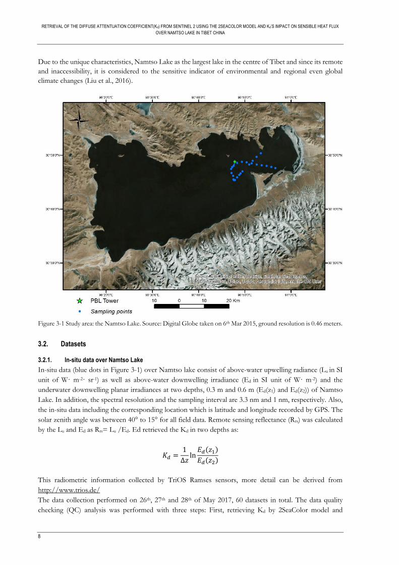
Due to the unique characteristics, Namtso Lake as the largest lake in the centre of Tibet and since its remote

and inaccessibility, it is considered to the sensitive indicator of environmental and regional even global

climate changes (Liu et al., 2016).

Figure 3-1 Study area: the Namtso Lake. Source: Digital Globe taken on 6th Mar 2015, ground resolution is 0.46 meters.

3.2. Datasets

3.2.1. In-situ data over Namtso Lake

In-situ data (blue dots in Figure 3-1) over Namtso lake consist of above-water upwelling radiance (Lu in SI

unit of W· m-2· sr-1) as well as above-water downwelling irradiance (Ed in SI unit of W· m-2) and the

underwater downwelling planar irradiances at two depths, 0.3 m and 0.6 m (Ed(z1) and Ed(z2)) of Namtso

Lake. In addition, the spectral resolution and the sampling interval are 3.3 nm and 1 nm, respectively. Also,

the in-situ data including the corresponding location which is latitude and longitude recorded by GPS. The

solar zenith angle was between 40° to 15° for all field data. Remote sensing reflectance (Rrs) was calculated

by the Lu and Ed as Rrs= Lu /Ed. Ed retrieved the Kd in two depths as:

𝐾𝑑 =1

∆𝑧ln

𝐸𝑑(𝑧1)

𝐸𝑑(𝑧2)

This radiometric information collected by TriOS Ramses sensors, more detail can be derived from

http://www.trios.de/

The data collection performed on 26th, 27th and 28th of May 2017, 60 datasets in total. The data quality

checking (QC) analysis was performed with three steps: First, retrieving Kd by 2SeaColor model and

http://www.trios.de/



9

validating by the field Kd data. Second, inspecting if the shapes of the outliers are abnormal or turbulent.

Third, deleting the turbulent data. According to the result of the quality check, 17 datasets were selected for

the further analysis.

The Lu and Ed values recorded by TriOS Ramses sensors equal to the diffuse and direct of the natural solar

radiation. Thus, the Lu and Ed values depended strongly on the weather condition when the measurement

executed. Table 3-2 shows the information of field data collection. The maximum values of Lu and Ed could

reach 21.55 mW·m-2nm-1 sr-1, and 1249.77 mW·m-2nm-1 and the minimum could reach 0.51 mW·m-2nm-1

sr-1 and 57.27 mW·m-2nm-1 during sunny midday among all the measurements. These radiance and irradiance

values indicated that the solar radiation intensity over the Namtso lake in the summer season is strong. In

general, the Ed(λ) spectra has a high magnitude in the blue-green region. The spectra of Kd(λ) (Figure 5-1)

is flat at the wavelength smaller than 700 nm and increase at the NIR band because the water molecules

have a strong absorption effect at NIR. During the in-situ data collection, the solar zenith angle of Namtso

Lake ranges from 49.25º~12.55 º.

Table 3-2 Field measurements.

Sampling date Sampling time

(GMT+8)

Number

of points

Number

of points

(after QC)

Weather condition

26th May 2017 10:07-14:57 14 4 Cloudy

27th May 2017 11:18-14:55 36 13 Cloudy

28th May 2017 10:51-12:55 10 0 Cloudy

Total / 60 17 /

3.2.2. Sentinel 2 MSI (S2 MSI) data and atmospheric correction

S2 MSI data has proven to be suitable for calculation of the water reflectance and thus retrieval of the water

quality variables (Vanhellemont & Ruddick, 2016). Therefore, the Sentinel 2 was selected as the input of

2SeaColor model to estimate Kd over Namtso Lake.

The corresponding S2 MSI data for validation should also be collected in 26th and 27th of May of 2017 with

minimal cloud cover. Unfortunately, only the data of 15th of May is available for the validation due to the

others are contaminated by cloud. Besides, because the TP features favourably low cloud cover during

winter, eight scenes of S2 MSI data from September to December of 2016 and 2017 were collected for

investigating the correlation between Kd and H. The dates of used S2 MSI data were shown in Table 3-3.

Also, the acquisition time of S2 MSI over Namsto Lake is around 04:41 to 04:45(UTC). The solar zenith

angle for all S2 data is ranging from 34° to 57°. In addition, a simple linear relationship was established to

shift wavelengths at 440 nm, 660 nm, 700 nm, and 780 nm of the field data to the corresponding wavelengths

at 443 nm, 665 nm, 705 nm, and 783 nm of S2 data due to the different channel setting between S2 and

field radiometric measurements. The determination coefficients larger than 0.99 were selected for the further

analysis.

Table 3-3 The dates of used S2 MSI data.

Year 2016 2016 2016 2016 2017 2017 2017 2017

Month 10 10 12 12 9 10 10 12

day 18 28 6 16 27 17 22 1



10

The spatial resolution of S2 is dependent on the particular spectral band. The 10 m spatial resolution bands

are B2 (490 nm), B3 (560 nm), B4 (665 nm) and B8 (842 nm); The 20 m resolution bands are B5 (705 nm),

B6 (740 nm), B7 (783 nm), B8a (865 nm), B11 (1610 nm) and B12 (2190 nm); The 60 m resolution bands

are B1 (443 nm), B9 (940 nm) and B10 (1375 nm). Table 3-4 shows the detail of Sentinel 2 specification. In

addition, the level 1C product of Sentinel 2 MSI which gives the Top of Atmosphere (TOA) reflectance has

already performed the radiometric and geometric correction, and hence it was used in this research to derive

Kd. Besides, the lake was clipped into two tiles of S2 data when downloading from the S2 data hub and thus

mosaicking was performed. The pixel values of mosaic images are using the arithmetic mean of pixels for

the two tiles.

Table 3-4 S2 MSI Specification.

Spatial resolution (meters)

Revisit time (days)

SWATH width (km)

Spectral bands Spectral range

(nm)

10,20,60 5 290 13 443-2190

For the aquatic application earth observation, the atmospheric correction (AC) is indispensable. The AC of

S2 MSI data implemented by iCOR and Alcolite algorithm. Both these two AC algorithms are state-of-the-

art and designed for aquatic application among S2 dedicatedly. iCOR is a plugin embedded in the Sentinel

Application Platform (SNAP). SNAP is a software designedly developed by Telespazio Germany (TPZV)

on behalf of ESA for the processing and analyzing the Sentinel 2 series data. The other alternative AC

algorithm is Alcolite which can run in the Python environment. After performing the AC, the level 2A

product was derived. The level 2A product includes the main output of Bottom of Atmosphere (BOA)

corrected reflectance product and the additional product of an Aerosol Optical Thickness (AOT) map, a

Water Vapor (WV) map etc.

The details of these two AC algorithms could be found in the part of Methodology.

3.2.3. Meteorological and Land Surface Temperature (LST) data

One of the objectives of this study is looking for the relation between Kd and H. However; it is hard to

observe the relation between Kd and H directly due to the dynamic nature of the water surface and

atmosphere. Hence, in order to analyse the relation between Kd and H, the study of the relation between

Kd and Lake Surface Temperature (LST) was first performed.

To begin with, there are several substitutes for the LST data such as (1) interpolating the surface temperature

form the automatic weather stations (AWS) which can provide the Namtso Lake surface temperature, (2)

using mathematical models to calculate the LST data from S2 MSI, (3) using the MODIS LST data directly.

However, with considering the temporal and spatial resolution as well as the amount of data processing, the

MODIS LST data was selected to perform the analysis.

The MODIS instrument onboard the Terra and Aqua spacecrafts. They provide global coverage every day

in 36 discrete spectral bands with viewing swath width of 2330 km. Terra’s/Aqua’s sun-synchronous, the

near-polar circular orbit is timed to cross the equator from north to south/south to north

(descending/ascending node) at approximately 10:30 a.m./p.m. local time. Additionally, some previous

studies (Xiao et al., 2013; Crosman & Horel, 2009) showed that MODIS/Terra LST product could provide

a better performance in terms of determination coefficient, bias, and RMSE than the MODIS/Aqua

product. Also given the amount of data processing, the level 2 LST MODIS/Terra version 6 product

(MOD11_L2), therefore, with the corresponding acquisition dates of Sentinel 2 were collected and

processed for this study. It has to be mentioned that the level 2 MODIS products were swath data without

geolocation system. Hence, the level 2 product was georeferenced and projected by ENVI plugin, MODIS

Conversion Toolkit (MCTK) 2.1.7, developed by Devin White. The MCTK released on GitHub



11

https://github.com/dawhite/MCTK. The LST MODIS/Terra product was reprojected onto

WGS84/UTM Zone 46N which was corresponding to S2 data. More information could be found in the

User’s Guide of MCTK.

The overpass time of MODIS recorded in coordinated universal time (UTC). MODIS/Terra LST products

provided two times (daytime and night time) per day measurements (Hu, Brunsell, Monaghan, Barlage, &

Wilhelmi, 2014). The MODIS/Terra overpass time for Namtso Lake is about 04:05 to 05:25 (UTC)

(daytime) and 15:40 to 16:45 (UTC) (night-time) in the study period, respectively. Concerning the acquisition

time of S2 MSI, the daytime MODIS/Terra product was selected for the further analysis. However, the

daytime MODIS/Terra product on the days of 18th October.2016, 28th October.2016, 16th October.2016,

and 1st December.2017 were not available because of the cloud contamination, thus, the night-time

MODIS/Terra products instead as the proxies.

The spatial resolution of MOD11_L2 product is 1 km. Due to the size of the Namtso Lake (L: 65 km, W:

40 km), the resolution of the MOD11_L2 product is acceptable. The MOD11_L2 product is the result of

the split-window method described by Zhengming Wan & Dozier (1996) and filtered with the MODIS

Cloud Mask products (MOD35 L2).

The meteorological data include wind speed (U) and near-surface air temperature (Ta) at the reference height

of 2.7 m which were derived from planetary boundary layer (PBL) tower (30°48'53.44"N 90°47'49.72"E,

green star in Figure 3-1) installed by the Nam Co Monitoring and Research Station for Multisphere, which

was established by the Institute of Tibetan Plateau Research, Chinese Academy of Sciences (Ma et al., 2014).

The wind speed and near-surface air temperature are measured at 05:00 (UTC) which is corresponding to

the acquisition time of S2 data.

https://github.com/dawhite/MCTK



12

4. METHODOLOGY

4.1. Flowchart of methodology

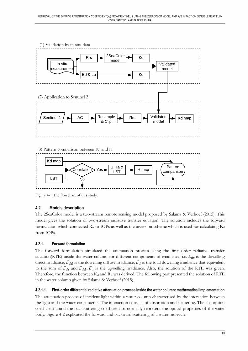
Figure 4-1 showed the overview of this study. Apparently, this study divided into three parts.

The first part concentrates on validating the 2SeaColor model by the in-situ data. Remote sensing reflectance

(Rrs) was inputted to the 2SeaColor model and then produced the Kd. Further, compared Kd produced by

2SeaColor model to Kd form in-situ data, consequently, the 2Seacolor model was validated by the in-situ

measurements.

The second part focuses on dealing with the Sentinel 2 images and applying the 2SeaColor model to calculate

the Kd of Namtso Lake. In addition, the validated 2SeaColor model applies to the Sentinel 2 images to

produce the Kd map over Namtso Lake. Certainly, the validation of Kd map estimated by the combination

of Sentinel 2 and the 2SeaColor model by the in-situ measurements could also be performed.

The third part is trying to establish a relationship between Kd and H to test the physical mechanism that

how Kd impacts on H. This step achieved by first investigating the correlation between Kd and lake surface

temperature (LST). Next, utilising the wind speed (U) and near-surface air temperature to calculate the H.

At last, the spatial and temporal patterns were analysed between Kd and H.

Kd in this context specifies the Kd at a wavelength of 490 nm, namely Kd (490). Because Kd as an apparent

optical property (AOP) determined by such factors as viewing illumination geometries and inelastic

scattering, thus, Kd is not constant with depth. However, as long as Kd at the adopted wavelength (490 nm),

the effect exerted by these factors are too small to consider compared to the overall measurement errors (

Zhang & Fell, 2007).



13

Figure 4-1 The flowchart of this study.

4.2. Models description

The 2SeaColor model is a two-stream remote sensing model proposed by Salama & Verhoef (2015). This

model gives the solution of two-stream radiative transfer equation. The solution includes the forward

formulation which connected Rrs to IOPs as well as the inversion scheme which is used for calculating Kd

from IOPs.

4.2.1. Forward formulation

The forward formulation simulated the attenuation process using the first order radiative transfer

equation(RTE) inside the water column for different components of irradiance, i.e. 𝐸𝑑𝑠 is the dowelling

direct irradiance, 𝐸𝑑𝑑 is the dowelling diffuse irradiance, 𝐸𝑑 is the total dowelling irradiance that equivalent

to the sum of 𝐸𝑑𝑠 and 𝐸𝑑𝑑 , 𝐸𝑢 is the upwelling irradiance. Also, the solution of the RTE was given.

Therefore, the function between Kd and Rrs was derived. The following part presented the solution of RTE

in the water column given by Salama & Verhoef (2015).

4.2.1.1. First-order differential radiative attenuation process inside the water column: mathematical implementation

The attenuation process of incident light within a water column characterised by the interaction between

the light and the water constituents. The interaction consists of absorption and scattering. The absorption

coefficient a and the backscattering coefficient bb normally represent the optical properties of the water

body. Figure 4-2 explicated the forward and backward scattering of a water molecule.

(1) Validation by in-situ data

(2) Application to Sentinel 2

(3) Pattern comparison between Kd and H



14

Figure 4-2 The scattering of a water molecule.

The radiative transfer equation described below (Duntley, 1942; Duntley, 1963):

d𝐸𝑑𝑑

dz= −𝑠′𝐸𝑑𝑠 + 𝛼𝐸𝑑𝑑 − 𝜎

d𝐸𝑢

dz= s𝐸𝑑𝑠 + 𝜎𝐸𝑑𝑑 − 𝛼𝐸𝑢

where 𝑘, 𝑠′, s , 𝛼, and 𝜎 are the attenuation coefficients for different irradiance components. These

components are listed in the Table 4-1 below. Table 4-1 The coefficients description in the attenuation process.

Coefficients Definition Equation

𝑘 The extinction coefficient m-1 𝑘 = 𝑐 𝜇𝑠⁄

𝑠′ Forward scattering for direct

sunlight s′ = 𝑏𝑓 𝜇𝑠⁄

s Backscattering direct for direct

sunlight s = 𝑏𝑏 𝜇𝑠⁄

𝛼 The diffuse extinction coefficient 𝛼 = 2𝑎 + 2𝑏𝑏

𝜎 The diffuse backward scattering

coefficient 𝜎 = 𝑏𝑏

c The extinction coefficient 𝑐 = 𝑎 + 𝑏

𝜇𝑠 Cosine of solar zenith angle

beneath the water 𝜇𝑠 = cos 𝜃𝑠

The diffuse attenuation coefficient, Kd, for the direct and diffuse light was described by the following

differential equation as:

Incident light

Backward

Forward

Water molecule

(1)



15

𝐾𝑑 =1

𝐸𝑑

d𝐸𝑑

dz

According to the solution of Eq.(1) given by Salama & Verhoef (2015), the function was shown below.

𝐾𝑑 =((𝑘 − 𝑠′)𝐸𝑑𝑠 + 𝛼 ∙ 𝐸𝑑𝑑 − 𝜎 ∙ 𝐸𝑢)

𝐸𝑑

where

𝐸𝑑 = 𝐸𝑑𝑑 + 𝐸𝑑𝑠

The 𝑟∞ and 𝑟𝑠𝑑∞ are the bi-hemispherical reflectance for the semi-infinite medium and the directional-

hemispherical reflectance of the semi-infinite medium. It is given by:

𝑟∞ =𝑥

1 + 𝑥 + √1 + 2𝑥

𝑟𝑠𝑑∞ =

√1 + 2𝑥 − 1

√1 + 2𝑥 + cos 𝜃𝑠

where x =𝑏𝑏

𝑎.

Therefore, the Kd was characterized by the IOPs. In addition,

R(0) =𝐸𝑢(0)

𝐸𝑑(0)=

𝑟∞ ∙ 𝐸𝑑𝑑(0) + 𝑟𝑠𝑑∞ ∙ 𝐸𝑑𝑠(0)

𝐸𝑑(0)

described the irradiance reflectance just beneath the water surface (R(0)). And then the R(0) converted to

the Rrs just above the water (Mobley, 1994):

𝑅𝑟𝑠 =0.52𝑅(0)

𝑄 − 1.7𝑅(0)

where Q is the Radiance-irradiance transfer coefficient which equals 3.25 in steradian (sr) under sunny

conditions (Lee et al., 2002).

Hereafter, the function between Rrs and Kd was established.

4.2.1.2. Forward scattering of suspended particles

The suspended particles normally present a peaked forward scattering which is different from the water molecules. The schematic diagram of the suspend particulate showed in Figure 4-3. In general, the

reflectance only related to the x which equals 𝑏𝑏

𝑎. This would imply that the forward scattering is not taken

into accounted the attenuation and backscattering. However, one can imagine that a proportion of the forward scattering still diffused and attenuated. Therefore, the 2SeaColor model consider the forward scattering component as a non-scattered flux in the attenuation process through similarity transformation (Hulst, 1981).

(2)

(3)

(4)

(5)

(6)

(7)

(8)



16

Figure 4-3 The scattering for a suspended particle.

4.2.2. Inversion scheme

The original 2SeaColor model proceeds through the assumption of the water molecule are the only

contributor to absorption of incident light in a water column within Near Infrared (NIR). Meanwhile, if x

was obtained through the relationship of Rrs and x, the bb at NIR can be calculated. The bb values at shorter

wavelengths then obtained by bio-optical model. Therefore, a can be calculated from the bb and x and thus,

only backscattering coefficient should be parameterized. Recently, this model improved by Yu et al. (2016)

using a parameterization of(Salama, Dekker, Su, Mannaerts, & Verhoef, 2009; Salama & Shen, 2010). Instead

of parameterising the bb, the improved 2SeaColor model parameterised the absorption coefficient of

chlorophyll( 𝛼𝜑) and combination of CDOM and non-algae (𝛼𝑑𝑔). The inversion scheme (Figure 4-4)

started by firstly inputting the initial values. Subsequently, the spectral optimization was employed to

simulate the Rrs through a nonlinear curve fitting based on the calculation of the minimum sum of squared

differences. The parameterization showed below.

𝑏𝑏 = 𝑏𝑏𝑝(𝜆0)(𝜆0

𝜆)𝑌

𝛼𝜑(𝜆) = 𝛼0(𝜆) + 𝛼1(𝜆)ln[(𝛼𝜑(440))]𝛼𝜑(440)

𝛼𝑑𝑔(𝜆) = 𝛼𝑑𝑔(𝜆0)𝑒−𝑆(𝜆−𝜆0)

where Y is the spectral slope of suspended particulates, and S is the spectral slope of the combination of

CDOM and non-algae. Note Y is ranging from 0.3 to 1.7 (Lee, Du, et al., 2005). S is ranged between 0.011

and 0.019 nm-1, and an average value of 0.015 nm-1 is adopted in this study (Lee et al., 2002).

Incident light

Backward

Forward

Suspended particulate

(9)

(10)

(11)



17

Figure 4-4 Inversion scheme of 2SeaColor model.

4.3. Atmospheric correction (AC) for Sentinel 2 data

AC for the coastal, transitional, and inland water application is a challenge due to the average ocean colour

AC algorithms normally neglect surface level change, adjacency effects, and non-Lambertian surface

reflection. Whereas iCOR and Alcolite are the state-of-the-art AC algorithm specify application of water

which released on 8th of August 2017 and 18th July 2017, respectively. These two AC algorithms are going

to be unfolded sequentially.

iCOR was originally designed for the airborne hyperspectral imagery. iCOR perform AC in following steps:

(1) identify the water and land pixels, and the land pixels are used for the generation of AOT, (2) adjacency

correction performed by SIMEC (Similarity Environment Correction), and (3) MODTRAN 5 (Berk et al.,

2006) Look Up Tables (LUT) was used to perform the AC. The strength of iCOR is that it can recognize if

a target pixel is a water or land and then performs a dedicated correction (Sindy Sterckx et al., 2015). In

addition, the extra module, SIMEC (Similarity Environment Correction), which can remove the

contamination of water pixels from the light of adjacency land and vegetation pixels (S Sterckx, Knaeps,

Kratzer, & Ruddick, 2014). Three output files of iCOR contain: (1) all the spectra at 60m spatial resolution,

(2) only bands with originally 20m spatial resolution and (3) only bands with originally 10m spatial resolution.

More information could be found in the iCOR manual: http://ec2-54-149-255-197.us-west-

2.compute.amazonaws.com/icor/manual/iCORpluginUserManual_v1.8.pdf.

Alcolite is an AC algorithm which can provide simple and fast processing for the Landsat 8 and S2 data.

Alcolite execute atmospheric correction in two steps: (1) after Rayleigh scattering correction using the 6SV

code (Vermote et al., 2006) to generate the LUT and (2) an aerosol correction based on the assumption of

black SWIR bands over water due to the pure water molecules absorption and multiple scattering aerosol

reflectance spectra(Vanhellemont & Ruddick, 2016). The resolution of output images is user-defined. It is

worthy to mention that the Alcolite is a very powerful algorithm which can produce the product of, i.e. Rrs,



18

chlorophyll-a concentration, SPM, turbidity, Quasi-Analytical Algorithm (Lee, Darecki, et al., 2005) which

including IOPs and Kd.

In this paper, the 10m and 60m resolution outputs of AC algorithms were used to compare to the AC

algorithm performance. Besides, this paper also evaluates the influence of different resolution to the AC

accuracy. The nearest neighbour of up-sampling (interpolation) method and down-sampling (aggregation)

method was adopted. The finer resolution product, 10m, allows more information of image is presenting

and the coarser resolution product, 60m, provides a shorter processing time. Therefore, these two resolution

products which have the best performance was selected for computing Kd.

4.4. Data analysis and accuracy assessment

To illustrate the performance of these models, there are four statistical parameters are planning present for

the retrieved Kd (490) from the model result and known Kd (490) from in-situ data. The five statistical

parameters are the root mean square error (RMSE), mean of absolute relative-differences (rMAD), slope

and intercept of the linear regression as well as the square of correlation coefficient R2. The RMSE and

rMAD expressed as:

RMSE = √∑(𝑑𝑒𝑟𝑖𝑣𝑒𝑑 − 𝑘𝑛𝑜𝑤𝑛)2

𝑁

rMAD = ∑|1 −

𝑑𝑒𝑟𝑖𝑣𝑒𝑑𝑟𝑎𝑛𝑔𝑒 |

𝑁× 100%

where N is the number of the observations. The slope and intercept are computed by model-II (Laws, 1997)

regression. Clearly, for the perfect goodness-of-fit between retrieved and known Kd (490) should have

RMSE=0, rMAD = 0, slope = 1, intercept = 0 and R2 = 1.

It is inevitable that validation of the Kd map produced by application of best model from Sentinel 2. The

accuracy assessment also represents the four statistical parameters.

4.5. Verification by Case 2 Regional Coast Colour (C2RCC) algorithm

The 2SeaColor model was verified by the C2RCC algorithm. Doerffer & Schiller, (2007) pioneered the

development of the C2RCC algorithm for MERIS using the neural network technique. The C2RCC

algorithm performed the AC and derived IOPs based on over five million cases of water types that generated

by neural networks. The C2RCC also gives the Kd at the wavelength of 489 nm that employed in this thesis

to verify the 2SeaColor model. C2RCC is applicable for all the ocean colour sensors, i.e. Sentinel 3 OLCI,

Sentinel 2 MSI, MERIS and SeaWiFS. C2RCC was widely validated by numerous of researchers, and it can

access by ESA’ s Sentinel toolbox, SNAP. The detail of the atmospheric correction and IOPs retrieval is

illustrated by Brockmann et al., (2016).

4.6. The correlation analysis for Kd and H

From a physical view, the Kd impacts on the LST, and consequently on H. However, it is hard to observe

the impaction. Therefore, the correlation analysis between Kd and H performed by firstly, correlating the Kd

and MODIS LST product, and secondly by analysing the spatial dependency relationship between Kd and

H.

(13)

(12)



19

4.6.1. The temporal correlation analysis for Kd and LST

The LST product was georeferenced and projected to share the same geographical and projection coordinate

with the Kd map produced by 2SeaColor model. Also, the values of not a number (NaN) in the LST product

was masked out. In addition, the correlation analysis executed only for the water pixels, thus, the Kd values

ranging from 0 to 2 m-1 were selected to define the water pixels.

The correlation coefficient, R, was computed by using

R =∑ ∑ (𝐴𝑚𝑛 − �̅�)(𝐵𝑚𝑛 − �̅�)𝑛𝑚

√(∑ ∑ (𝐴𝑚𝑛 − �̅�)2𝑛𝑚 )(∑ ∑ (𝐵𝑚𝑛 − �̅�)2)𝑛𝑚

where A and B are the matrices (images) that share the same size, i.e. m rows and n columns (pixel location).

Besides, �̅� , and �̅� are the mean value in A and B. Hence, the basic operator what Eq. (14) calculated is, the

difference, for every water pixel location, between the value in that pixel and the mean value of the whole

image (Figure 4-5). Besides, the denominator presents a kind of normalization where the pixel value

difference within every individual image. In summary, R, in this context, showed the overall correlation of

all pixels regardless the spatial aspect. Therefore, R can indicate the relationship of two images with respect

to temporal variations.

Figure 4-5 Schematic diagram of temporal correlation.

4.6.2. The spatial correlation analysis for Kd and LST

The spatial correlation analysis computed the correlation coefficient for every water pixel of the LST daytime

products (6th December.2016, 27th September.2017, 17th October.2017, and 22nd October.2017) and

corresponded Kd maps (Figure 4-6). Therefore, the result is a map of correlation coefficient which can

present the spatial relationship.

(14)



20

Figure 4-6 Schematic diagram of spatial correlation.

4.6.3. The correlation analysis for Kd and H

H was calculated as:

H = 𝐶𝑝𝜌𝑎𝐶𝐻𝑈(𝑇𝑠 − 𝑇𝑎)

where 𝐶𝑝 (1009 J*kg-1*K-1 at 10 ℃) is the specific heat of air, 𝜌𝑎 (0.73 kg*m-3 at TP) is the air density, 𝐶𝐻

is the bulk transfer coefficient which adopt 1.834 *10-3 at reference height above the lake according to

Kondo, (1975), and U is the wind speed. Ts and Ta are the lake surface temperature and air temperature

obtained from PBL tower at reference height, respectively.

The correlation coefficient for the Kd and H was calculated only for the daytime LST time series because

this correlation coefficient was based on a pixel which could induce turbulence if the entire time series was

counted.

(15)



21

5. RESULTS

5.1. Remote sensing reflectance and Kd from in-situ measurement

The remote sensing reflectance (Rrs) and the diffuse attenuation coefficient (Kd) calculated from field data

(Ed and Lu) are presented in Figure 5-1. The peak in Rrs (Figure 5-1 (a)) can be found at blue-green band

region. On the contrary, the extremely low values of Rrs were caused by the intense absorption of pure water

molecules in the red and NIR (Majozi, Suhyb, Bernard, Harper, & Ghirmai, 2014) (Ruddick, De Cauwer,

Park, & Moore, 2006). Looking at the Kd (Figure 5-1 (b)), the valley at blue-green band represent the

attenuation of incident light is not strong, while the peak in Figure 5-1 (b) at NIR band also showed the

consistent result with Rrs as almost all incident light was absorbed at NIR band.

Figure 5-1 Field measurements of Rrs and Kd spectrum curves (black) with their mean (red) and standard deviation (blue) values.

Table 5-1 showed the mean values and standard deviations for Kd as an auxiliary for understanding the

spectrum. Therefore, these spectrum features suggested most of the sites of water are relatively clear without

so much presence of phytoplankton, SPM, and CDOM. This preliminary speculation is similar to the result

of the previous research (Yong, Liping, Junbo, Jianting, & Xiao, 2012).

The Rrs spectrum curves highly fluctuate over the visible and near-infrared area. In addition, the Kd spectrum

curves also showed high variation with respect to magnitude and shape. Variations of these spectrum curve

mainly due to the undulating weather condition which means high frequency switching of cloudy and clear

skies at the time the spectra were collected. Besides, the optically important water constituents spatial and

temporal distribution also accounts for the fluctuations. As a matter of fact, the underwater topography and

river supply may also exert an unexpected effect on the Rrs and Kd variations.

Table 5-1 The average values (mean) and standard deviations (STD) for the Rrs and Kd of selected wavelengths over Namtso Lake.

Wavelength 400 450 500 550 600 650 700 750 800

Kd_Mean 0.61 0.61 0.61 0.64 0.80 0.94 1.19 2.97 2.75

Kd_STD 0.39 0.44 0.47 0.51 0.56 0.60 0.65 0.93 0.91



22

5.2. Validation for Kd retrieved by 2SeaColor model

5.2.1. Validating Kd by in-situ measurements

2SeaColor model (Salama & Verhoef, 2015) are used to estimate the Kd of Namtso Lake. Figure 5-2 showed

the scattering plot of derived Kd (490nm) from the model against known Kd (490nm) from field

measurements. The only input of 2SeaColor model is the remote sensing reflectance from field

measurements.

The Kd produced by 2SeaColor possesses a relatively large deviation in turbid water where Kd>0.2 m-1 (T.

Zhang & Fell, 2007). Besides, the model underestimated the Kd when the Kd values greater than 0.5 m-1 as

the slope (=0.765) is more than 20% off unity. Looking at the R2 (=0.765) and the relative error, rMAD

(=12.32%), which demonstrate the 2SeaColor model is relatively reliable. Besides, the intercept (=0.07) from

the linear regression between modelled and known Kd of 2SeaColor model is close to zero. The intercept

represented a small linear offset between the modelled Kd and known Kd. Therefore, it can conclude from

above results the 2SeaColor model performs acceptably despite the underestimation.

Figure 5-2 Derived Kd (490nm) from 2SeaColor model against known Kd (490nm) from field measurements.

5.2.2. Validating Kd by Convolved in-situ measurements

The instrument spectral response functions (SRFs) or relative spectral responses describe the quantum

efficiency of an instrument at specific wavelengths over the range of a spectral band (Fleming, 2006).

Therefore, the Rrs measured by TriOS Ramses sensors (in situ data) should be matched up the S2 MSI,

namely convolution. The convolution achieved by the following formula

𝑅𝑟𝑠(𝑖)(𝑐𝑜𝑛𝑣𝑜𝑙𝑣𝑒𝑑) =∫ (𝑅𝑟𝑠(𝑗)(𝑖𝑛−𝑠𝑖𝑡𝑢)(𝜆) ∗ 𝑆𝑅𝐹𝑠𝑖(𝜆))𝑑𝜆

𝜆2

𝜆1

∫ 𝑆𝑅𝐹𝑠𝑖𝜆2

𝜆1(𝜆)𝑑𝜆

where i is the number of bands of Sentinel 2, j is the site's number of in situ data as well as the 𝜆1and 𝜆2 are

adopt 400nm and 800nm thereby.

Figure 5-3 showed the validation of 2SeaColor model by convolved in-situ Rrs measurements. Obviously,

the 2SeaColor model performed better after convolution. But Kd is also dispersed as increasing of the known

Kd. The R2 was slightly higher than the result of field modelled. The rMAD and slope were diminished.

Also, the almost accordance slope was given by 2SeaColor model after convolution. In summary, the

convolution provided an overall better result for the modelling.



23

Figure 5-3 Derived Kd (490nm) from 2SeaColor model against known Kd (490nm) from convolved field measurements.

5.3. Estimating Kd from Sentinel 2 image

In order to further illustrate the potential of the 2SeaColor model for remote sensing Kd, the Sentinel 2 data

were tested to validate the applicability. The processing of Sentinel 2 proceeds to the atmospheric correction.

Simultaneously, convolving the in situ remote sensing reflectance to Sentinel 2 MSI spectra. After

convolution, the newly produced in situ remote sensing reflectance data transfer the view of TriOS Ramses

sensors to the view of Sentinel 2 MSI. Sequentially, mapping Kd by applied 2SeaColor model to atmospheric

corrected Sentinel 2 image. At last, validating the map of Kd generated from 2SeaColor model by the in situ

Kd measurements.

5.3.1. Atmospheric correction (AC) for Sentinel 2 image

The weather was cloudy when collecting the field data which resulted in the large errors occurred for both

iCOR and Alcolite algorithms. However, iCOR has better performance for some of field data sites.

The comparison of iCOR and Alcolite AC algorithms in 10m and 60m resolution of one site showed in

Figure 5-4. Blue lines represent Rrs from iCOR algorithm (the output of iCOR is water leaving reflectance,

and thus it has to transfer to Rrs divided by pi hereby). Red lines stand for Rrs from the Alcolite algorithm.

And black is the convolved field measured Rrs data. Additionally, solid lines represent 10m spatial resolution

while dash lines stand for the 60m spatial resolution. The statistical parameters are shown in Table 5-2 for

an insight of the assessment of AC algorithms.

Apparently, the spectra of iCOR in 60m spatial resolution is much closer than the others to the field

measurements from the Figure 5-4. And only the iCOR in 60m spectra describes the trend of 443nm and

490nm (Rrs(443)>Rrs(490)) in the same way with the in situ Rrs. Besides, the R2 represents the strength of

correlation between field data and AC results regarding shape, and the iCOR in 60m have the largest value

means the iCOR in 60m own the strongest relationship with the field data compared to the others. With

respect to RMSE and rMAD, the spectra of iCOR in 60m also possesses the smallest values (RMSE=0.0019.

rMAD=19.2977%). The rMAD of iCOR in 10m and Alcolite in 10m are excess 100% which signifies the

Rrs values between rMAD of iCOR in 10m as well as Alcolite in 10m and field measured are not in the same

magnitude. Therefore, the iCOR at 60m was adopted to perform AC.

It has to be mentioned that iCOR in 60m AC algorithm is not performed as good as this one site for all the

field data, it is considered, however, adequate for this study.



24

Figure 5-4 Assessment of AC algorithms with the convolved field measured Rrs data in 10m and 60m spatial resolutions.

Table 5-2 Statistical parameters of the iCOR and Alcolite AC algorithms in 10m and 60m spatial resolutions.

iCOR_10 iCOR_60 Alcolite_10 Alcolite_60

R2 0.94 0.99 0.55 0.51

RMSE 0.0238 0.0019 0.0167 0.0097

rMAD 225.36 19.30 164.17 81.95

5.3.2. Mapping Kd by 2SeaColor model

Figure 5-5 depicted the Kd maps at the wavelength of 490 nm from October to December of 2016 and 2017

of Namtso Lake. It must mention that the easily observed discrete horizontal line was created by mosaicking

in Figure 5-5 (a) and (e). Also, the relatively conspicuous strip area was the S2 camera trace for all the images

showed in Figure 5-5. Besides, there were several small abnormal areas in 28th Oct.2016, 6th December.2016

and 16th December.2016 caused by clouds. Thus, these three effects should ignore when one analysing the

spatial and temporal patterns of Kd.

The spatial characteristics could be observed, as nearshore waters presented a high Kd value, particularly at

the north and west of the lake, whereas, the offshore waters showed a much lower Kd value. The values of

Kd on 28 October 2016 (Figure 5-5 (b)), however, exhibited an inverse spatial pattern, as the high values

can be found in the middle of the lake, while, only the west of the lake presented a low Kd value. Besides,

the Kd on 27 September 2017 (Figure 5-5 (e)) also showed a different pattern that Kd is high except the

south of the lake.

As for the temporal pattern of Kd, there are no enormous variations within the whole time series regardless

the Figure 5-5 (b) and Figure 5-5 (e). However, one can conclude that Kd in December is lower than the

October if neglects the data limitation.



25

Figure 5-5 Kd (490nm) maps estimated by 2SeaColor model using atmospheric corrected S2 data for Namtso Lake on eight days: (a) 18th Oct. 2016, (b) 28th Oct.2016, (c) 6th Dec.2016, (d) 16th Dec.2016, (e) 27th Sept.2017, (f) 17th Oct.2017, (g) 22nd Oct.2017, and (h) 1st Dec.2017.



26

5.4. Verification

The statistic variables were Kd for C2RCC and 2SeaColor models on three days were shown in Table 5-3.

The field measurement also shown as the indicator of model performance. Apparently, according to the

mean values of C2RCC and 2SeaColor on the day of 28th Oct 2016, the 2SeaColor has a better

performance since it is closed to the mean value of the field data, while the mean values of C2RCC are

smaller than the 2Seacolor’s on all the three days which means the C2RCC could underestimate the Kd. In

addition, the stand deviations of 2SeaColor model are much greater than C2RCC’s could indicate the Kd

produced by 2SeaColor model is more dispersion. The stand deviation and dynamic range (DR) of

2SeaColor, however, closed to the field data on 28th Oct 2016 represented Kd of 28th Oct 2016 and field

data share the similar range.

Overall, the 2SeaColor has better performance while the C2RCC is underestimated the Kd.

Table 5-3 The statistic variables of Kd for C2RCC and 2SeaColor models on three days. DR represents dynamic range (N=10).

28th Oct.2016 15th May.2017 22nd Oct.2017

Statistics Mean STD DR Mean STD DR Mean STD DR C2RCC 0.106 0.038 0.129 0.162 0.031 0.118 0.095 0.017 0.065

2SeaColor 1.069 0.445 1.366 2.344 0.915 2.524 0.442 0.142 0.580

Field data Mean: 0.752, STD: 0.471, DR: 1.151 collected on 25th May.2017.



27

5.5. Kd and sensible heat flux (H)

5.5.1. The temporal correlation analysis for Kd and LST

The relation between Kd and LST with respect to temporal variation was quantified by the correlation

coefficient (R) showed in Figure 5-6. R took the contributions for all the pixels into consideration regardless

the spatial distribution, thus, it represented the temporal correlation ignored the spatial influence. One can

observe that R contained both positive and negative values from Figure 5-6. This inconsistency is able to

attribute to the replacement of night-time LST product because night-time LST presented an inverse

behaviour compared to the daytime LST, i.e. the lake surface temperature is lower than the land temperature

at daytime while it is opposed at night time. Besides, the only R of 22nd October 2017 was greater than 0.5,

while others are relatively low. This may imply lake surface temperature is not determined by diffuse

attenuation coefficient exclusively, further, it is hard to isolate the effect of light attenuation to the lake

surface temperature. In addition, the low correlation coefficients could also attribute to (1) the different

acquisition time between S2 and MODIS, (2) the algorithm of LST computation, since there is no in-situ

lake surface temperature was collected in the Namtso Lake, thus, the LST data from MODIS was not

validated.

Figure 5-6 The correlation coefficients between Kd and LST.

5.5.2. The spatial correlation analysis for Kd and LST

Every pixel value in correlation (r) map (Figure 5-7) were computed by two columns of data as (1) the pixel

value of LST for all the daytime series (2) the pixel value of Kd for all the same time series and location with

LST. Therefore, the correlation map presented the spatial characteristics of the relationship between Kd and

LST. Apparently, it is easy to observe that the most areas of the lake own a high correlation coefficient

except the south of the lake. The correlation almost zero in the south of the lake indicated that the Kd and

LST are almost uncorrelated. Besides, there is a small parcel presented a high negative correlation in the

southwest part of the lake.



28

Figure 5-7 The correlation coefficient (r) map for Kd and LST.

5.5.3. The correlation analysis for Kd and H

According to the Eq. (15), the sensible heat flux (H) and the correlation coefficients were (Co) computed

and was shown in Table 5-4. The correlation coefficient for Kd and LST (Ts) at the single site, PBL tower

site, is 0.93 which indicate that Kd and LST have a strong positive relationship, while the correlation

coefficient for the Kd and H is -0.85 which present a strong negative relationship. The correlation coefficient

for the Kd and the difference between Ts and Ta (△T) is -0.66, the correlation coefficient between the wind

speed (U) and H is 0.98 indicated that the wind speed predominates the sensible heat flux.

Table 5-4 The meteorological data, computed H and the correlation coefficients.

Date U(m/s) Ta(K) Ts(K) Ts-

Ta(K) Kd(m-1) H(W·m-2) Co_Kd_Ts Co_Kd_△T Co_Kd_H Co_H_U

Daytime

6th.10.2016 7.6 271.2 277.6 6.5 0.23 64.9

0.93 -0.66 -0.85 0.99 27th.09.2017 1.0 282.7 285.9 3.3 0.50 4.2 17th.10.2017 0.9 278.4 283.6 5.2 0.35 6.4 22nd.12.2017 2.7 274.7 283.2 8.5 0.34 30.1

Night time

18th.10.2016 2.3 276.1 282.4 6.3 0.04 19.4 -0.12 0.79 0.52 0.6 28th.10.2016 2.6 269.0 278.9 9.9 1.15 33.9

16th.12.2016 10.6 272.8 275.4 2.5 0.19 35.6



29

6. DISCUSSION

In this study, the 2SeaColor model was employed to estimate the Kd over Namtso Lake. The model was

validated by in situ data. Further, the sensible heat flux (H) was computed, sequentially, the correlation

analysis was conducted between Kd and H.

6.1. Assessment of 2SeaColor model

6.1.1. Validation

It is found that 2SeaColor model using the convolved Rrs performed much better than before convolution.

This is mainly because convolution averaged the error. The slight discrepancy of Rrs was enhanced when

propagated to IOPs, i.e. absorption coefficient and backscattering coefficient, through the spectrum

optimisation. The equations (Eq. (9) (10) (11)) employed by spectrum optimisation was an exponential

function which leads to the enhancement of IOPs. The absorption coefficient (a) and backscattering

coefficient (bb) increased by 44.7% and 35.8% averagely for all the in-situ measurements. The ratio x of

backscattering coefficient to the absorption coefficient present an ensemble effect of light attenuation, thus,

x was reduced due to the increasing of IOPs. Therefore, it indicated that more energy of incident light was

attenuated by the water constituents, consequently, Kd produced by 2SeaColor increased.

The significant improvement in terms of slope can be understood that the convolution plays a critical role

in the Kd retrieval. Spectral response functions define the spectral band position and extent, thus, it is

normally considered as the pivotal source of uncertainty and compatibility for different sensors (D’Odorico,

Gonsamo, Damm, & Schaepman, 2013; Teillet, Fedosejevs, Thome, & Barker, 2007). Although the

convolution is by no means affected the overall spectral shape of Rrs, it has a significant impact on Kd.

The impact also reflects that AC should be very careful to be treated (Wang, Son, & Shi, 2009).

This result showed the 2SeaColor model was stable and applicable to the alpine Lake Namtso using S2 data.

Also, it was consistent with previous studies that validation of 2SeaColor model in Naivasha Lake (Suhyb

Salama & Verhoef, 2015) and Yangtze estuary (Yu et al., 2016).

6.1.2. Verification

Basically, 2SeaColor model and C2RCC model have a different range of the estimated Kd which could

mainly due the employed the totally different AC algorithm. The only input of the 2SeaColor model is the

remote sensing reflectance that derived from AC, hence, AC is attributed to the enormous difference

between the Kd estimated by 2SeaColor model and C2RCC model. In addition, the mean value and stand

deviation of 2SeaColor on the 15th May 2017 in Table 5-3 is greater than the field data, which indicated on

that day, the 2SeaColor model could overestimate the Kd. Therefore, it is concluded that both of the

2SeaColor model and C2RCC model are not given a very good agreement, while comparably, the

2SeaColor model explicated a better performance.

6.2. The spatial and temporal characteristics of Kd in Namtso Lake

The Kd is an apparent optical property that depends on the illumination-viewing geometry. Since 2SeaColor

model takes into accounts the solar zenith angle, thus, solar zenith angle is not considered as a factor that

affects the Kd variation. Besides, Kd is the quantification of the underwater light availability, and it is

determined by the and IOPs of optically active water constituents. In general, typical optically active water

constituents such as chlorophyll-a (Chl-a), dissolved organic matter (DOM), suspended particulate matter

(SPM) mainly influence the Kd variability (Mobley, 1994; Liu et al., 2010; Cairo, Barbosa, de Moraes Novo,

& do Carmo Calijuri, 2017). Morel & Antoine (1994) suggested Kd rises from the concentration of Chl-a

caused by bio-optically induced radiative heating.



30

The geographical information explains the distribution of optically active water constituents in Namtso

Lake. About 60 rivers flowing into the Namtso Lake and most of these rivers are small rivers. These small

rivers distributed in the west and south of the lake (Wang et al., 2010). Additionally, Wang et al., (2010)

indicated the large perennial rivers are drain into the western and eastern parts of the lake.

The underwater topography has an important effect on the SPM enrichment. Bathymetric surgery was

conducted to understanding the underwater topography features (Wang et al., 2009). There is a large deep

flat area in the centre of the lake, and the deepest depth could reach 98.9m. Besides, the lake floor slope

with a sharp gradient was found at the north and south of the lake where mountains are situated, while the

west and east have a gentle slope where the alluvial fans are distributed caused by the large perennial rivers.

Thus, it has a potential of SPM enrichment in Nmatso Lake.

Liu et al. (2010) suggested that high Chl-a was found in the northern offshore water of Namtso Lake in

September 2005. But the average value of Chl-a was 0.46 μg*L-1 which are still low. Lami et al. (2010)

indicated the concentration of pigments was increased during the recent years. It can attribute to the

extended growing season of algae caused by climate warming. Nima et al. (2016) found that the

concentration of Chl-a was very low (0.1 μg*L-1) although the sample was collected during the productive

season, May to September.

To sum up, Kd in Namtso Lake is dominated by SPM rather than by the concentration of Chl-a. The

northeast and the northwest of the lake showed a high Kd value. This is mainly because the sand and silt

transported by the rivers were enriched in the northeast and northwest of the Namtso Lake. The sand and

silt could view as the SPM which often explicit a strong forward scattering. The strong forward scattering

considered as the non-scattering fluxes by a 2SeaColor model that results in the Kd increased. In fact, the

Kd values are still low compared to other study areas (Lee, Du, et al., 2005; Zhang & Fell, 2007; Simon &

Shanmugam, 2016) that indicate the Namtso Lake is a reasonable turbid alpine lake that Kd varied with time

(Vollenweider, 1982; Nima et al., 2016).

As for the temporal pattern, due to Namtso Lake located in the TP which is known as extremely cold in

winter, little activity of water, also phytoplankton (Calijuri, Dos Santos, & Jati, 2002) and suspended

particulates was presented. Therefore, the Kd explicated a similar pattern of variation in December. In

another hand, Kd in September and October, especially on the day of 28th of October 2016 presented a

much greater spatial variation than the Kd in December. The greater spatial variations of Kd on 28th of

October 2016 could attribute to the large △T value (9.9 K). It is reported that the largest △T appeared in

the autumn and winter in Namtso Lake (Haginoya et al., 2009). Due to the significant difference between

air temperature and water surface temperature, the deeper water is requested to exchange energy with the

upper layer water in order to compensate the large difference between lake surface temperature and air

temperature. This request leads to the enhancement of the stratification and convection of the upper layer

of the lake. This result could compare to the study on the Labrador Sea (Wu et al., 2007) that the mixed-

layer depth reduced by 20-50% after the external heating induced to the water body.

6.3. The relationship between Kd and H

Increased Kd represents more incoming solar radiation being attenuated by the upper layer of the water

body (Giardino, Pepe, Brivio, Ghezzi, & Zilioli, 2001; Zhang et al., 2015; Chen, Zhang, Xing, Ishizaka, &

Yu, 2017). The attenuated solar energy could result in the increasing of the water surface temperature. It is

known that surface temperature is one of the factors that controlled the sensible heat flux. Previous studies

(Wu et al., 2007; Wu, Platt, Tang, & Sathyendranath, 2008)demonstrated the bio-optically induced Kd

variations impact on the water surface temperature. However, rare studies concentrated on the question: to

what extent, the Kd dominate the LST or H? This study conducted the correlation analysis between Kd and

LST for the whole Namtso Lake, also the correlation between Kd and H for one point of the Namtso Lake.



31

6.3.1. The temporal correlation analysis of Kd and LST

R, temporal correlation coefficient in this context, represents the correlation between instantaneous

variables Kd and LST for all the pixels and for every single acquisition time of S2 and MODIS. Figure 5-6

indicates that it is not conclusive that the Kd and LST are correlated within the eight selected dates due to

the low correlation coefficients. This result could attribute to (1) Kd and H are instantaneous variables, thus,

different acquisition time of S2 and MODIS could lead to the uncorrelation, (2) R explicated the overall

effect (refer to Eq.14) of the map of Kd and LST which could eliminate some interconnections between Kd

and H. Additionally, the correlation coefficients of 17th and 22nd October 2017 are relatively high compared

to other dates. The reason for the high temporal correlation coefficient needs more investigation. In

summary, the Kd and LST are varied in these eight acquisition time, so the results are not enough to draw a

conclusion.

6.3.2. The spatial correlation analysis of Kd and LST

The spatial correlation coefficients, r, represent the correspondence for every pixel between Kd map and

LST map for the four daytime products. The result (Figure 5-7) of spatial correlation analysis showed Kd is

significantly positively correlated with LST except for the south part of the lake. The result indicated that

the Kd and LST shared the same pattern within the specified time series for the most part of the lake. The

weak correlation at the south part of the lake could attribute that the values of Kd at the south of the lake

on the 27th September.2017 was lower than the other three days. Besides, a small area with the extreme high

negative correlation coefficient occurred in the bottom left corner on account of the clouds on the day of

6th December.2016. The edge of the clouds presents a much higher Kd values than the water due to the

strong attenuation effect by the clouds, thus, the Kd of the edge of clouds was very high. The centre of the

clouds is no value in the Kd map because the Rrs is too high to input to the 2SeaColor model.

Previous studies (Wu et al., 2008; Giardino et al., 2001; Wu et al., 2007) normally focus on how LST varied

with Kd instead of the correlation analysis.

In summary, LST is the boundary that connects the turbulent air and the turbulent water. Generally, LST

dependent on sensible heat flux that the LST air-water heat flux feedback is around 20 W*m-1*K-1 for the

seawater (Hausmann, Czaja, & Marshall, 2016; Frankignoul, Czaja, & L’Heveder, 1998), considering, also,

the high correlation between Kd and LST presented in Figure 5-7 that indicated Kd is related to H. However,

solar radiation, wind speed, horizontal advection and stability of the water column also determined the LST

(Emery & Yu, 1997). Therefore, one should consider not only the relationship between Kd and LST but

also consider the other parameters of air-water interaction if one performs the correlation analysis between

light attenuation and water surface temperature.

6.3.3. Kd and H

The correlation coefficients of environment variables among the air-water interaction are listed in Table 5-

4 above. The correlation coefficients (Kd & Ts, Kd & △T, Kd & H and H & U) only calculate from the PBL

site which site contains the meteorological data. The daytime correlation coefficients computed by the

daytime LST products on 6th December.2016, 27th September.2017, 17th October.2017, and 22nd

October.2017 as well as the corresponding Kd map produced by 2SeaColor model. The night time

correlation coefficients were calculated in the same way. Table 5-4 showed the low coefficients of night time

simply because the Kd and LST product is not acquired at the same time as Kd maps were acquired at

daytime, but LST products were acquired at night time.

For daytime correlation coefficients, the significant negative correlation coefficient (=-0.85) between Kd and

H indicated that an increase of Kd results in a decrease of H. This is mainly because when Kd increased,

more energy was tapped in the water lead to restricting the heat releasing, thus, the H decreased. Wind speed

has the most important contribution of H according to the largest correlation coefficient (=0.98) between

U and H. In another word, wind speed plays a more significant role in the heat transfer compared to Kd on



32

the Namtso Lake. The result of the physical control of sensible heat flux was consistent with the small lake

near the Namtso Lake investigated by Wang et al., 2015 and Wang et al., 2017.

Actually, the Eq.15 simplify the calculation of H that only consider the Ta and Ts and wind speed. But the

real situation is much more complicated than the Eq.15 described. H is also related to the atmospheric

stability and the energy exchange via atmosphere advection between the lake and land surfaces (Lofgren &

Zhu, 2000).

6.4. The limitations

The field measurement was performed on 25th May 2017 while the acquisition date of S2 matchup data was

on 15th May 2017. The difference between data from the two days could induce the major uncertainty. In

addition, estimation of the uncertainty generated form IOPs inversion scheme play an important role in the

assessment of the ocean colour retrieval algorithm (Salama et al., 2011; Lee et al., 2010). In this study,

however, IOPs such as absorption coefficient and backscattering coefficient are not measured could result

in the errors originated from the inversion scheme in 2SeaColor model cannot observe. Besides, the

atmospheric correction should select carefully.

General errors may originate from the highly dynamic water turbulence and subpixel effect, and the human-

induced error when performing the in-situ measurements. Besides, satellite data limited by clouds, also the

number of in-situ measurements and the meteorological data that used to calculate the H is excepted cover

the whole lake.

Therefore, based on the limitation mentioned above, the following recommendations were given (1) field

measurements should cover more areas of the lake, (2) the wind speed data and the air temperature are

supposed to use the dedicated model to estimate in order to provide the wind speed map and air temperature

map of the lake, (3) the studied time series should extend.

7. CONCLUSIONS

In this study, the 2SeaColor model was employed to estimate the diffuse attenuation coefficient for the

underwater downward irradiance in combination with S2 data over Namtso Lake in TP. Based on the results

and analysis above, the following conclusions were drawn:

1. The 2SeaColor model is capable of providing a relatively accurate estimation of Kd that is ranging from 0

to 2 m-1 in Namtso Lake.

2. The northeast and northwest of the nearshore waters of the lake presented a higher Kd value than the

offshore of the lake. This spatial distribution of Kd is attributed to the SPM transported by the inflowed

river was enriched in the river mouth. Therefore, the Kd mainly controlled by SPM in Namtso Lake. The

temporal distribution of Kd explicated a similar pattern because it is cold months during the studies time

series which result in the little activity of the optically significant water constituents.

3. It is not conclusive that the Kd and LST are temporally correlated within the eight studied time series. As

for the spatial correlation between Kd and LST, however, Kd of most of the lake areas are significantly

correlated with LST.

4. The correlation coefficient between Kd and H is -0.85 for one site in the lake for four days’ measurements.

Therefore, Kd has an enormous potential to predict the LST or H despite the influential mechanism should

vastly investigate.

35

LIST OF REFERENCES

Austin, R. W., & Petzold, T. J. (1981). The Determination of the Diffuse Attenuation Coefficient of Sea Water Using the Coastal Zone Color Scanner BT - Oceanography from Space. In J. F. R. Gower (Ed.) (pp. 239–256). Boston, MA: Springer US. https://doi.org/10.1007/978-1-4613-3315-9_29

Berk, A., Anderson, G. P., Acharya, P. K., Bernstein, L. S., Muratov, L., Lee, J., … Hoke, M. L. (2006). MODTRAN5: 2006 update. In Proc. SPIE (Vol. 6233, p. 62331F).

Brockmann, C., Doerffer, R., Peters, M., Kerstin, S., Embacher, S., & Ruescas, A. (2016). Evolution of the C2RCC neural network for Sentinel 2 and 3 for the retrieval of ocean colour products in normal and extreme optically complex waters. In Living Planet Symposium (Vol. 740, p. 54).

Brutsaert, W. (1982). Energy Fluxes at the Earth’s Surface. In Evaporation into the Atmosphere (pp. 128–153). Dordrecht: Springer Netherlands. https://doi.org/10.1007/978-94-017-1497-6_6

Cairo, C. T., Barbosa, C. C. F., de Moraes Novo, E. M. L., & do Carmo Calijuri, M. (2017). Spatial and seasonal variation in diffuse attenuation coefficients of downward irradiance at Ibitinga Reservoir, São Paulo, Brazil. Hydrobiologia, 784(1), 265–282. https://doi.org/10.1007/s10750-016-2883-7

Calijuri, M. C., Dos Santos, A. C. A., & Jati, S. (2002). Temporal changes in the phytoplankton community structure in a tropical and eutrophic reservoir (Barra Bonita, S.P.--Brazil). Journal of Plankton Research, 24(7), 617–634. https://doi.org/10.1093/plankt/24.7.617

Chang, G. C., & Dickey, T. D. (2004). Coastal ocean optical influences on solar transmission and radiant heating rate. Journal of Geophysical Research, 109(C1), C01020. https://doi.org/10.1029/2003JC001821

Chen, J., Zhang, X., Xing, X., Ishizaka, J., & Yu, Z. (2017). A Spectrally Selective Attenuation Mechanism-Based KparAlgorithm for Biomass Heating Effect Simulation in the Open Ocean. Journal of Geophysical Research: Oceans, 9370–9386. https://doi.org/10.1002/2017JC013101

Crosman, E. T., & Horel, J. D. (2009). MODIS-derived surface temperature of the Great Salt Lake. Remote Sensing of Environment, 113(1), 73–81. https://doi.org/10.1016/J.RSE.2008.08.013

D’Odorico, P., Gonsamo, A., Damm, A., & Schaepman, M. E. (2013). Experimental evaluation of sentinel-2 spectral response functions for NDVI time-series continuity. IEEE Transactions on Geoscience and Remote Sensing, 51(3), 1336–1348. https://doi.org/10.1109/TGRS.2012.2235447

Dekker, A. G., Vos, R. J., & Peters, S. W. M. (2002). Analytical algorithms for lake water TSM estimation for retrospective analyses of TM and SPOT sensor data. International Journal of Remote Sensing, 23(1), 15–35. https://doi.org/10.1080/01431160010006917

Denman, K. L. (1973). A Time-Dependent Model of the Upper Ocean. Journal of Physical Oceanography, 3(2), 173–184. https://doi.org/10.1175/1520-0485(1973)003<0173:ATDMOT>2.0.CO;2

Doerffer, R., & Schiller, H. (2007). The MERIS Case 2 water algorithm. International Journal of Remote Sensing, 28(3–4), 517–535. https://doi.org/10.1080/01431160600821127

Duntley, S. Q. (1942). The Optical Properties of Diffusing Materials. Journal of the Optical Society of America, 32(2), 61. https://doi.org/10.1364/JOSA.32.000061

Duntley, S. Q. (1963). Light in the Sea*. Journal of the Optical Society of America, 53(2), 214. https://doi.org/10.1364/JOSA.53.000214

Emery, W. J., & Yu, Y. (1997). Satellite sea surface temperature patterns. International Journal of Remote Sensing, 18(2), 323–334. https://doi.org/10.1080/014311697219097

Fleming, D. J. (2006). EFFECT OF RELATIVE SPECTRAL RESPONSE ON MULTI-SPECTRAL MEASUREMENTS AND NDVI FROM DIFFERENT REMOTE SENSING SYSTEMS. University of Maryland. Retrieved from https://drum.lib.umd.edu/bitstream/handle/1903/3313/umi-umd-3147.pdf;jsessionid=802C75B9DBFC0BB835BEAD2288E23339?sequence=1

Frankignoul, C., Czaja, A., & L’Heveder, B. (1998). Air–Sea Feedback in the North Atlantic and Surface Boundary Conditions for Ocean Models. Journal of Climate, 11(9), 2310–2324. https://doi.org/10.1175/1520-0442(1998)011<2310:ASFITN>2.0.CO;2

Giardino, C., Pepe, M., Brivio, P. A., Ghezzi, P., & Zilioli, E. (2001). Detecting chlorophyll, Secchi disk depth and surface temperature in a sub-alpine lake using Landsat imagery. Science of The Total Environment, 268(1–3), 19–29. https://doi.org/10.1016/S0048-9697(00)00692-6

Glasgow, H. B., Burkholder, J. M., Reed, R. E., Lewitus, A. J., & Kleinman, J. E. (2004). Real-time remote monitoring of water quality: a review of current applications, and advancements in sensor, telemetry, and computing technologies. Journal of Experimental Marine Biology and Ecology, 300(1), 409–448.

Guan, Z. H., Chen, C. Y., Ou, Y. X., Fan, Y. Q., Zhang, Y. S., Chen, Z. M., … Zhang, M. T. (1984).

36

Rivers and lakes in Tibet. Science and Technology Press, Beijing (in Chinese). Haginoya, S., Fujii, H., Kuwagata, T., Xu, J., Ishigooka, Y., Kang, S., & Zhang, Y. (2009). Air-Lake

Interaction Features Found in Heat and Water Exchanges over Nam Co on the Tibetan Plateau. Sola, 5(55279), 172–175. https://doi.org/10.2151/sola.2009-044

Hausmann, U., Czaja, A., & Marshall, J. (2016). Estimates of air-sea feedbacks on sea surface temperature anomalies in the Southern Ocean. Journal of Climate, 29(2), 439–454. https://doi.org/10.1175/JCLI-D-15-0015.1

Hu, L., Brunsell, N. A., Monaghan, A. J., Barlage, M., & Wilhelmi, O. V. (2014). How can we use MODIS land surface temperature to validate long-term urban model simulations? Journal of Geophysical Research: Atmospheres, 119(6), 3185–3201. https://doi.org/10.1002/2013JD021101

Hulst, H. C. van de (Hendrik C. (1981). Light scattering by small particles. Dover Publications. Imberger, J., & Patterson, J. C. (1980). Dynamic Reservoir Simulation Model-DYRESM: 5. Transport models for

inland and coastal waters. New York: Academic press. Ke, C.-Q., Tao, A.-Q., & Jin, X. (2013). Variability in the ice phenology of Nam Co Lake in central Tibet

from scanning multichannel microwave radiometer and special sensor microwave/imager: 1978 to 2013. Journal of Applied Remote Sensing, 7(1), 73477. https://doi.org/10.1117/1.JRS.7.073477

Kondo, J. (1975). Air-sea bulk transfer coefficients in diabatic conditions. Boundary-Layer Meteorology, 9(1), 91–112. https://doi.org/10.1007/BF00232256

Kratzer, S., Brockmann, C., & Moore, G. (2008). Using MERIS full resolution data to monitor coastal waters — A case study from Himmerfjärden, a fjord-like bay in the northwestern Baltic Sea. Remote Sensing of Environment, 112(5), 2284–2300. https://doi.org/10.1016/j.rse.2007.10.006

Kropáček, J., Maussion, F., Chen, F., Hoerz, S., & Hochschild, V. (2013). Analysis of ice phenology of lakes on the Tibetan Plateau from MODIS data. The Cryosphere, 7(1), 287–301. https://doi.org/10.5194/tc-7-287-2013

Lami, A., Turner, S., Musazzi, S., Gerli, S., Guilizzoni, P., Rose, N. L., … Yang, R. (2010). Sedimentary evidence for recent increases in production in Tibetan plateau lakes. Hydrobiologia, 648(1), 175–187. https://doi.org/10.1007/s10750-010-0263-2

Laws, E. A. (1997). Mathematical methods for oceanographers: An introduction. John Wiley & Sons. Lee, Z.-P., Darecki, M., Carder, K. L., Davis, C. O., Stramski, D., & Rhea, W. J. (2005). Diffuse

attenuation coefficient of downwelling irradiance: An evaluation of remote sensing methods. Journal of Geophysical Research, 110(C2), C02017. https://doi.org/10.1029/2004JC002573

Lee, Z., Du, K., & Arnone, R. (2005). A model for the diffuse attenuation coefficient of downwelling irradiance. Journal of Geophysical Research, 110(C2), C02016. https://doi.org/10.1029/2004JC002275

Lee, Z., Arnone, R., Hu, C., Werdell, P. J., & Lubac, B. (2010). Uncertainties of optical parameters and their propagations in an analytical ocean color inversion algorithm. Applied Optics, 49(3), 369. https://doi.org/10.1364/AO.49.000369

Lee, Z., Carder, K. L., & Arnone, R. A. (2002). Deriving inherent optical properties from water color: a multiband quasi-analytical algorithm for optically deep waters. Applied Optics, 41(27), 5755. https://doi.org/10.1364/AO.41.005755

Lee, Z., Darecki, M., Carder, K. L., Davis, C. O., Stramski, D., & Rhea, W. J. (2005). Diffuse attenuation coefficient of downwelling irradiance: An evaluation of remote sensing methods. Journal of Geophysical Research C: Oceans, 110(2), 1–9. https://doi.org/10.1029/2004JC002573

Liu, K., Liu, Y., Jiao, N., Zhu, L., Wang, J., Hu, A., & Liu, X. (2016). Vertical variation of bacterial community in Nam Co, a large stratified lake in central Tibetan Plateau. Antonie van Leeuwenhoek, International Journal of General and Molecular Microbiology, 109(10), 1323–1335. https://doi.org/10.1007/s10482-016-0731-4

Liu, X., & Chen, B. (2000). Climatic warming in the Tibetan Plateau during recent decades. International Journal of Climatology, 20(14), 1729–1742. https://doi.org/10.1002/1097-0088(20001130)20:14<1729::AID-JOC556>3.0.CO;2-Y

Liu, X., Yao, T., Kang, S., Jiao, N., Zeng, Y., & Liu, Y. (2010). Bacterial community of the largest Oligosaline Lake, Namco on the Tibetan plateau. Geomicrobiology Journal, 27(8), 669–682. https://doi.org/10.1080/01490450903528000

Lofgren, B. M., & Zhu, Y. (2000). Surface energy fluxes on the Great Lakes based on satellite-observed surface temperatures 1992 to 1995. Journal of Great Lakes Research, 26(3), 305–314. https://doi.org/10.1016/S0380-1330(00)70694-0

Loiselle, S. A., Bracchini, L., Cózar, A., Dattilo, A. M., Tognazzi, A., & Rossi, C. (2009). Variability in photobleaching yields and their related impacts on optical conditions in subtropical lakes. Journal of

37

Photochemistry and Photobiology B: Biology, 95(2), 129–137. https://doi.org/10.1016/j.jphotobiol.2009.02.002

Ma, Y., Zhu, Z., Zhong, L., Wang, B., Han, C., Wang, Z., … Hu, Z. (2014). Combining MODIS, AVHRR and in situ data for evapotranspiration estimation over heterogeneous landscape of the Tibetan Plateau. Atmospheric Chemistry and Physics, 14(3), 1507–1515. https://doi.org/10.5194/acp-14-1507-2014

Majozi, N. P., Suhyb, M., Bernard, S., Harper, D. M., & Ghirmai, M. (2014). Remote Sensing of Environment Remote sensing of euphotic depth in shallow tropical inland waters of Lake Naivasha using MERIS data. Remote Sensing of Environment, 148, 178–189. https://doi.org/10.1016/j.rse.2014.03.025

Mobley, C. D. (1994). Light and water: radiative transfer in natural waters. Academic press. Morel, A., & Antoine, D. (1994). Heating Rate within the Upper Ocean in Relation to its Bio–optical

State. Journal of Physical Oceanography, 24(7), 1652–1665. https://doi.org/10.1175/1520-0485(1994)024<1652:HRWTUO>2.0.CO;2

Nima, C., Hamre, B., Frette, Ø., Erga, S. R., Chen, Y.-C., Zhao, L., … Stamnes, J. J. (2016). Impact of particulate and dissolved material on light absorption properties in a High-Altitude Lake in Tibet, China. Hydrobiologia, 768(1), 63–79. https://doi.org/10.1007/s10750-015-2528-2

O’Reilly, J. E., Maritorena, S., Mitchell, B. G., Siegel, D. A., Carder, K. L., Garver, S. A., … McClain, C. (1998). Ocean color chlorophyll algorithms for SeaWiFS. Journal of Geophysical Research: Oceans, 103(C11), 24937–24953. https://doi.org/10.1029/98JC02160

Pu, H., Liu, D., Qu, J.-H., & Sun, D.-W. (2017). Applications of Imaging Spectrometry in Inland Water Quality Monitoring—a Review of Recent Developments. Water, Air, & Soil Pollution, 228(4), 131. https://doi.org/10.1007/s11270-017-3294-8

Read, J. S., Hamilton, D. P., Desai, A. R., Rose, K. C., MacIntyre, S., Lenters, J. D., … Wu, C. H. (2012). Lake-size dependency of wind shear and convection as controls on gas exchange. Geophysical Research Letters, 39(9), n/a-n/a. https://doi.org/10.1029/2012GL051886

Read, J. S., Rose, K. C., Winslow, L. A., & Read, E. K. (2015). A method for estimating the diffuse attenuation coefficient (KdPAR) from paired temperature sensors. Limnology and Oceanography: Methods, 13(2), 53–61. https://doi.org/10.1002/lom3.10006

Ruddick, K. G., De Cauwer, V., Park, Y.-J., & Moore, G. (2006). Seaborne measurements of near infrared water-leaving reflectance: The similarity spectrum for turbid waters. Limnol. Oceanogr, 51(2), 1167–1179. Retrieved from http://ir.polytechnic.edu.na/bitstream/handle/10628/216/ve.pdf?sequence=1&isAllowed=y

Salama, M. S., Dekker, A., Su, Z., Mannaerts, C. M., & Verhoef, W. (2009). Deriving inherent optical properties and associated inversion-uncertainties in the Dutch Lakes. Hydrology and Earth System Sciences, 13(7), 1113–1121. https://doi.org/10.5194/hess-13-1113-2009

Salama, M. S., Mélin, F., & Van der Velde, R. (2011). Ensemble uncertainty of inherent optical properties. Optics Express, 19(18), 16772. https://doi.org/10.1364/OE.19.016772

Salama, M. S., & Shen, F. (2010). Simultaneous atmospheric correction and quantification of suspended particulate matters from orbital and geostationary earth observation sensors. Estuarine, Coastal and Shelf Science, 86(3), 499–511. https://doi.org/10.1016/J.ECSS.2009.10.001

Salama, M. S., & Stein, A. (2009). Error decomposition and estimation of inherent optical properties. Applied Optics, 48(26), 4947. https://doi.org/10.1364/AO.48.004947

Salama, M. S., & Verhoef, W. (2015). Two-stream remote sensing model for water quality mapping: 2SeaColor. Remote Sensing of Environment, 157, 111–122. https://doi.org/10.1016/j.rse.2014.07.022

Simon, A., & Shanmugam, P. (2016). Estimation of the spectral diffuse attenuation coefficient of downwelling irradiance in inland and coastal waters from hyperspectral remote sensing data: Validation with experimental data. International Journal of Applied Earth Observation and Geoinformation, 49, 117–125. https://doi.org/10.1016/j.jag.2016.02.003

Sterckx, S., Knaeps, E., Adriaensen, S., Reusen, I., Keukelaere, L. De, & Hunter, P. (2015). Opera : an Atmospheric Correction for Land and Water. Proceedings of the Sentinel-3 for Science Workshop, (1), 3–6. Retrieved from http://odnature.naturalsciences.be/downloads/publications/Sterckxetal_2015S3Forscience_finalv2-1.pdf

Sterckx, S., Knaeps, E., Kratzer, S., & Ruddick, K. (2014). SIMilarity Environment Correction (SIMEC) applied to MERIS data over inland and coastal waters. Remote Sensing of Environment (Vol. 157). https://doi.org/10.1016/j.rse.2014.06.017

38

Stramska, M., & Zuzewicz, A. (2013). Influence of the parametrization of water optical properties on the modelled sea surface temperature in the Baltic Sea**This work was supported by the SatBałtyk project funded by the European Union through the European Regional Development Fund (contract No. POIG.01.01.02-22-011/09 entitled “The Satellite Monitoring of the Baltic Sea Environment”). Oceanologia, 55(1), 53–76. https://doi.org/10.5697/oc.55-1.053

Su, Z., Levizzani, V., Rott, H., Wagner, W., Salama, M., Parodi, G., & Wang, L. (2011). Treatise on Water Science. (Peter Wilderer, Ed.). Oxford Aacdemic Press. Retrieved from https://blackboard.utwente.nl/bbcswebdav/pid-1013114-dt-content-rid-2369044_2/courses/M17-WREM-102/Documents/Remote sensing of water quality References Su etal 2011/42_TOWS_EOWC_Elsevier2011.pdf

Teillet, P. M., Fedosejevs, G., Thome, K. J., & Barker, J. L. (2007). Impacts of spectral band difference effects on radiometric cross-calibration between satellite sensors in the solar-reflective spectral domain. Remote Sensing of Environment, 110(3), 393–409. https://doi.org/10.1016/j.rse.2007.03.003

Tiwari, S. P., & Shanmugam, P. (2014). A Robust Algorithm to Determine Diffuse Attenuation Coefficient of Downwelling Irradiance From Satellite Data in Coastal Oceanic Waters. IEEE Journal of Selected Topics in Applied Earth Observations and Remote Sensing, 7(5), 1616–1622. https://doi.org/10.1109/JSTARS.2013.2282938

Vanhellemont, Q., & Ruddick, K. (2016). ACOLITE FOR SENTINEL-2: AQUATIC APPLICATIONS OF MSI IMAGERY. ESA Special Publication, 9–13. Retrieved from https://odnature.naturalsciences.be/downloads/publications/vanhellemontruddick_esa_lps2016_coastalapplications_final_header.pdf

Vermote, E., Tanré, D., Deuzé, J. L., Herman, M., Morcrette, J. J., & Kotchenova, S. Y. (2006). Second Simulation of a Satellite Signal in the Solar Spectrum -Vector (6SV). Retrieved from http://6s.ltdri.org/files/tutorial/6S_Manual_Part_1.pdf

Vollenweider, R. A. (1982). Eutrophication of waters : monitoring, assessment and control. (O. for E. C. and Development, Ed.). Paris : [Washington, D.C: Organisation for Economic Co-operation and Development ; Sold by OECD Publications and Information Center].

Vorosmarty, C. J., McIntyre, P. B., Gessner, M. O., Dudgeon, D., Prusevich, A., Green, P., … Davies, P. M. (2010). Global threats to human water security and river biodiversity. Nature, 467(7315), 555–561. Retrieved from http://dx.doi.org/10.1038/nature09440

Wang, B., Ma, Y., Chen, X., Ma, W., Su, Z., & Menenti, M. (2015). Observation and simulation of lake-air heat and water transfer processes in a high-altitude shallow lake on the Tibetan Plateau. Journal of Geophysical Research: Atmospheres, 120(24), 12327–12344. https://doi.org/10.1002/2015JD023863

Wang, B., Ma, Y., Ma, W., & Su, Z. (2017). Physical controls on half-hourly, daily, and monthly turbulent flux and energy budget over a high-altitude small lake on the Tibetan Plateau. Journal of Geophysical Research, 122(4), 2289–2303. https://doi.org/10.1002/2016JD026109

Wang, J., Zhu, L., Daut, G., Ju, J., Lin, X., Wang, Y., & Zhen, X. (2009). Investigation of bathymetry and water quality of Lake Nam Co, the largest lake on the central Tibetan Plateau, China. Limnology, 10(2), 149–158. https://doi.org/10.1007/s10201-009-0266-8

Wang, J., Zhu, L., Wang, Y., Ju, J., Xie, M., & Daut, G. (2010). Comparisons between the chemical compositions of lake water, inflowing river water, and lake sediment in Nam Co, central Tibetan Plateau, China and their controlling mechanisms. Journal of Great Lakes Research, 36(4), 587–595. https://doi.org/10.1016/j.jglr.2010.06.013

Wang, M., Son, S. H., & Shi, W. (2009). Evaluation of MODIS SWIR and NIR-SWIR atmospheric correction algorithms using SeaBASS data. Remote Sensing of Environment, 113(3), 635–644. https://doi.org/10.1016/j.rse.2008.11.005

Wu, Y., Platt, T., Tang, C., & Sathyendranath, S. (2008). Regional differences in the timing of the spring bloom in the Labrador Sea. Marine Ecology Progress Series, 355, 9–20. https://doi.org/10.3354/meps07233

Wu, Y., Tang, C. C. L., Sathyendranath, S., & Platt, T. (2007). The impact of bio-optical heating on the properties of the upper ocean: A sensitivity study using a 3-D circulation model for the Labrador Sea. Deep Sea Research Part II: Topical Studies in Oceanography, 54(23–26), 2630–2642. https://doi.org/10.1016/j.dsr2.2007.08.019

Xiao, F., Ling, F., Du, Y., Feng, Q., Yan, Y., & Chen, H. (2013). Evaluation of spatial-temporal dynamics in surface water temperature of Qinghai Lake from 2001 to 2010 by using MODIS data. Journal of Arid Land, 5(4), 452–464. https://doi.org/10.1007/s40333-013-0188-5

Yong, W., Liping, Z., Junbo, W., Jianting, J., & Xiao, L. (2012). The spatial distribution and sedimentary

39

processes of organic matter in surface sediments of Nam Co, Central Tibetan Plateau. Geography December, 5736, 4753–4764. https://doi.org/10.1007/s11434-012-5500-9

Yu, X., Salama, M. S., Shen, F., & Verhoef, W. (2016). Retrieval of the diffuse attenuation coefficient from GOCI images using the 2SeaColor model: A case study in the Yangtze Estuary. Remote Sensing of Environment, 175, 109–119. https://doi.org/10.1016/j.rse.2015.12.053

Zhang, R. H., Gao, C., Kang, X., Zhi, H., Wang, Z., & Feng, L. (2015). ENSO Modulations due to Interannual Variability of Freshwater Forcing and Ocean Biology-induced Heating in the Tropical Pacific. Scientific Reports, 5(November), 1–11. https://doi.org/10.1038/srep18506

Zhang, T., & Fell, F. (2007). An empirical algorithm for determining the diffuse attenuation coefficient K d in clear and turbid waters from spectral remote sensing reflectance. Limnology and Oceanography: Methods, 5(12), 457–462. https://doi.org/10.4319/lom.2007.5.457

Zheng, Z., Ren, J., Li, Y., Huang, C., Liu, G., Du, C., & Lyu, H. (2016). Remote sensing of diffuse attenuation coefficient patterns from Landsat 8 OLI imagery of turbid inland waters: A case study of Dongting Lake. Science of the Total Environment, 573, 39–54. https://doi.org/10.1016/j.scitotenv.2016.08.019

Zhengming Wan, & Dozier, J. (1996). A generalized split-window algorithm for retrieving land-surface temperature from space. IEEE Transactions on Geoscience and Remote Sensing, 34(4), 892–905. https://doi.org/10.1109/36.508406

Zhu, D. ., Meng, X. ., Zhao, X. ., Shao, Z. ., Feng, X. ., Yang, C. ., … Zhang, W. . (2004). On the Quaternary Environmental Evolution of Nam Co Area, Tibet. Beijing: Geology Press.