retrieval of equivalent currents by the use of an integral...

LUND UNIVERSITY

PO Box 117221 00 Lund+46 46-222 00 00

Retrieval of equivalent currents by the use of an integral representation and theextinction theorem --- radome applications

Persson, Kristin

2010

Link to publication

Citation for published version (APA):Persson, K. (2010). Retrieval of equivalent currents by the use of an integral representation and the extinctiontheorem --- radome applications. Department of Electrical and Information Technology, Lund University.

General rightsCopyright and moral rights for the publications made accessible in the public portal are retained by the authorsand/or other copyright owners and it is a condition of accessing publications that users recognise and abide by thelegal requirements associated with these rights.

• Users may download and print one copy of any publication from the public portal for the purpose of private studyor research. • You may not further distribute the material or use it for any profit-making activity or commercial gain • You may freely distribute the URL identifying the publication in the public portalTake down policyIf you believe that this document breaches copyright please contact us providing details, and we will removeaccess to the work immediately and investigate your claim.

http://portal.research.lu.se/portal/en/publications/retrieval-of-equivalent-currents-by-the-use-of-an-integral-representation-and-the-extinction-theorem--radome-applications(1eeb2710-7966-4e41-be63-c51aff2f0486).html

Retrieval o

f equ

ivalent cu

rrents b

y the u

se of an

integ

ral represen

tation

and

the extin

ction

theo

rem —

rado

me ap

plicatio

ns Department of Electrical and Information Technology,

Faculty of Engineering, LTH, Lund University, 2010.

Retrieval of equivalent currents bythe use of an integralrepresentation and the extinctiontheorem — radome applications

Kristin Persson

Series of licentiate and doctoral theses Department of Electrical and Information Technology

1654-790X No. 22

http://www.eit.lth.se

Kristin

Persso

n

Licentiate dissertation

Retrieval of equivalent currents bythe use of an integral

representation and the extinctiontheorem — radome applications

Kristin Persson

Licentiate Dissertation

Electromagnetic Theory

Lund University

Lund, Sweden

2010

Department of Electrical and Information TechnologyElectromagnetic TheoryLund UniversityP.O. Box 118, S-221 00 Lund, Sweden

Series of licentiate and doctoral thesesNo. 22ISSN 1654-790X

c© 2010 by Kristin Persson, except where otherwise stated.Printed in Sweden by Tryckeriet i E-huset, Lund University, Lund.January 2010

Abstract

The aim of this thesis is to solve an inverse source problem. The approach is basedon an integral representation together with the extinction theorem. Both a scalarand a full-wave integral representation are implemented and solved by a Method ofMoment procedure. The body of revolution enables usage of a Fourier transform toreduce the dimensions of the problem. A singular value decomposition is utilized tosuppress singular values in the inversion process. A nose-cone radome is diagnosed byrecreating the equivalent surface currents on its surface from measured near fields. Itis shown how the radome interacts with the field, creating beam deflection, patterndistortion, etc.. The phase shift of the field due to the transmission through theradome, i.e., the insertion phase delay, is visualized. Disturbances due to defects, notdetectable in the measured near field, are correctly localized by the equivalent surfacecurrents. The alteration of side and flash lobes, together with the introduction ofscattering due to the defects, are also visualized. Verification is made by comparisonbetween the calculated and measured far field.

Popularvetenskaplig sammanfattning (in Swedish)

Anvandningen av elektromagnetiska falt ar en naturlig del i det moderna samhallet.I var dagliga miljo ar vi beroende av informationen och energin som de elektro-magnetiska vagorna transporterar. Som exempel kan namnas mobiltelefonsamtal,uppvarmning av mat i mikrovagsugnen, anvandning av internet och radarover-vakning pa flygplatser.

For att konstruera en antenn sa att korrekta falt sands ut ar det viktigt att kunnastudera det elektromagnetiska faltets utseende pa antennytan. En sadan studie kanpeka pa var felaktigheter ar lokaliserade samt hjalpa till att optimera antennen.Falten pa ytan kan inte direkt matas upp. Ett sadant forsok resulterar i matfel pga.vaxelverkan mellan antennen och matproben. Istallet mats faltet upp en bit bortfran antennen och berakningar gors for att bestamma hur kallorna, det vill sagafalten pa antennytan, ser ut. Detta ar ett inverst kallproblem.

I denna avhandling loses det inversa kallproblemet med hjalp av en integralrep-resentation tillsammans med utslackningssatsen (eng. extinction theorem). Imple-menteringen baseras pa en momentkod (eng. Method of Moments). I artikel I–IIanvands en skalar integralrepresentation. I artikel III implementeras en vektorvardintegralrepresentation vilken tar hansyn till vaxelverkan mellan faltets komponen-ter. Det inversa problemet ar fel stallt, vilket innebar att sma fel i matdata kanforstarkas och ge upphov till stora felaktiga bidrag i kallbeskrivningen. Har minskasdenna paverkan genom att anvanda en singularvardesuppdelning (eng. SingularValue Decomposition, SVD) i inverteringsprocessen.

Metoden har anvants for att diagnostisera en radom (noskon som skyddar enradarantenn). En reflektorantenn innanfor en konformad radom alstrar ett elektro-magnetiskt falt. Det elektriska faltet mats upp pa en cylindrisk yta en bit utanforradomen i narfaltszonen, vid frekvenserna 8 − 12 GHz. Tre olika fall har studer-ats; ingen radom som tacker antennen, radomen pa plats, samt en defekt radomplacerad over antennen. Det uppmatta elektriska faltet ”backas” med hjalp avberakningar tillbaka till radomytan. Genom att studera tredimensionella bilder avfaltkomponenternas amplitud och fas pa radomytan, visas hur faltet forandras daradomen ar placerad over antennen. Bland annat minskar huvudloben, och sidloberuppkommer. Fasens forandring (eng. Insertion phase delay, IPD) ar ett satt attmata radomens prestanda vid tillverkning, och har visas en metod som har poten-tial att ersatta den idag vanliga manuella matningen.

Den defekta radomen har tva kopparbitar fastsatta pa ytan. Nar det upp-matta faltet studeras kan man se att nagot ar fel, men inte orsaken till felet. Dafaltet ”backas” syns defekternas placering tydligt. Man ser aven hur kopparbitarnaforandrar bakatloberna, samt att det uppkommer spridningseffekter. Metoden harverifierats genom en jamforelse med uppmatt fjarrfalt.

List of included papers

This dissertation consists of a General Introduction and the following scientific pa-pers:

I. K. Persson and M. Gustafsson. Reconstruction of equivalent currents using anear-field data transformation – with radome applications, Progress in Elec-tromagnetics Research, vol. 54, pp. 179–198, 2005.

II. K. Persson and M. Gustafsson. Reconstruction of equivalent currents using thescalar surface integral representation, Technical Report LUTEDX/(TEAT-7131), pp. 1–25, 2005, Department of Electrical and Information Technology,Lund University, Sweden. http://www.eit.lth.se

III. K. Persson, M. Gustafsson, and G. Kristensson. Reconstruction and visualiza-tion of equivalent currents on a radome surface using an integral representationformulation, Technical Report LUTEDX/(TEAT-7184), pp. 1–45, 2010, De-partment of Electrical and Information Technology, Lund University, Sweden.http://www.eit.lth.se1

Other publications by the author

IV. K. Persson and M. Gustafsson. Reconstruction of equivalent currents using anear-field data transformation - with radome applications, Technical ReportLUTEDX/(TEAT-7125), pp. 1–15, 2004, Department of Electrical and Infor-mation Technology, Lund University, Sweden.2


V. K. Persson and M. Gustafsson. Reconstruction of equivalent currents us-ing a near-field data transformation - with radome applications, ProceedingsEMB04, Computational Electromagnetics - Methods and Applications (EMB04), Goteborg, Sweden, pp. 124–131, October 18–19, 2004.

VI. K. Persson and M. Gustafsson. Near field to equivalent currents transfor-mation with radome applications, Proceedings International Symposium onElectromagnetic Theory, International Symposium on Electromagnetic The-ory (URSI EMTS 2004), Pisa, Italy, pp. 1122–1124, May 23–27, 2004.3

VII. K. Persson, M. Gustafsson, and G. Kristensson. Experimental validationof reconstructed equivalent currents on a radome, International Conferenceon Electromagnetic Near-Field Characterization & Imaging (ICONIC 2005),Barcelona, Spain, pp. 35-40, June 8–10, 2005.

1Submitted for publication.2This report is a longer and more detailed version of the publication in I.3Young Scientist Award.

VIII. K. Persson, M. Gustafsson, and G. Kristensson. Usage of a surface integralrepresentation to reconstruct equivalent currents - with radome applications,Proceedings of Radiovetenskap och kommunikation, Nordic Conference on Ra-dio Science and Communications (RVK 05), Linkoping, Sweden, June 14–16,2005.

IX. S. Nordebo, M. Gustafsson, K. Persson. Sensitivity analysis for antenna near-field imaging. IEEE Transactions on Signal Processing, vol. 55, no. 1, pp. 94-101, 2007.

Summary of included papers

Paper I - Reconstruction of equivalent currents using a near-field data transformation – with radome applications

This paper shows how the near-field amplitude of a scalar electric field can bereconstructed on a radome surface close to the source of radiation. The methodis based on a scalar surface integral representation together with the extinctiontheorem. The representation describes an inverse source problem with the scalarelectric field and its normal derivative on the radome surface as unknowns. Theexperimental set-up is axially symmetric, such that the complexity of the problemcan be reduced by employing a Fourier transform. The linear system is regularizedby the singular value decomposition (SVD). The measurement set-up consists ofa reflector antenna and a radome. The height of the radome corresponds to 29wavelength at 8 GHz. The electric near field is measured on a cylindrical surface.Three different configurations are considered in the frequency range 8 − 12 GHz:no radome, the radome, and the defect radome present. The defect radome hastwo copper plates attached to its surface. The formulation is first validated forsynthetic data and an error estimation is performed. It is then showed that themeasured electric field can be reconstructed on the radome surface in an accurateway, where e.g., the copper plates, not seen in the measured near field, are detected.The used technique is also verified by comparing the far field, calculated from thereconstructed fields, to measured far field.The author of this dissertation has carried out most of the analysis, and she isresponsible for the numerical simulations, and the writing of the paper.

Paper II - Reconstruction of equivalent currents using thescalar surface integral representation

This paper is a continuation of Paper I in the sense that the numerical analysisof the radome is investigated further. The phase of the electric field is taken intoaccount. The phase delay caused by the radome, referred to as insertion phase delay(IPD), is studied. It is also shown that the manufacturing errors, not shown in themeasured near-field data, can be focused and detected by reconstructing the phaseshift due to the propagation though the radome. Different ways of visualizing theresults are also discussed and presented in order to show which knowledge that canbe extracted from the measured near field.The author of this dissertation has carried out most of the analysis, and she isresponsible for the numerical simulations, and the writing of the paper.

Paper III - Reconstruction and visualization of equivalentcurrents on a radome surface using an integral representationformulation

In this paper, the inverse source problem is solved by utilizing a vector-valued in-tegral representation combined with a vector-valued integral equation originatingfrom the extinction theorem. The coupling between the components of the fieldsincreases the complexity of the problem. The problem is solved in a similar way asthe scalar case, i.e., the integral representation and equation are written as linearsystems and solved by a Method of Moment approach. An SVD is employed to in-vert the matrices and the singular values are suppressed to regularize the problem.The three radome configurations are investigated at 8 GHz, and all components ofthe measured field are now analyzed, i.e., both co- and cross components of theequivalent currents are reconstructed. It is shown in what way the radome changesthe radiation pattern and causes the main lobe to deflect. The copper plates at-tached to the radome alter the measured electric field. However, the cause of thedistortion is not seen in the near field. Here, it is shown that both components ofthe magnetic equivalent current can be used to localize these effects. The influenceof the radome on the phase of the field, i.e., the IPD, is also investigated. A calcula-tion of the thickness of the radome wall from the calculated IPD verifies the results.The results in this paper show that the method is promising and can eventually beemployed for industrial use.The author of this dissertation has carried out most of the analysis, and she isresponsible for the numerical simulations in parts, and the writing of the paper.

Acknowledgments

First and foremost, I would like to express my deep gratitude to my supervisorsProf. Gerhard Kristensson and Assoc. Prof. Mats Gustafsson. Without yourgreat knowledge within the area of electromagnetic theory, your guidance, and youreffort to always have time for discussions, I would not have made it this far. Itis an inspiration to take part of your positive spirit, eagerness to find intuitiveunderstanding of complex problems, and your remarkable stress hardiness.

The work reported in this thesis was made possible by a grant from the SwedishDefense Material Administration, and their support is gratefully acknowledged. Iam indebted to Saab Bofors Dynamics and Applied Composites AB, for providingmeasurement data. In discussing the concepts of radomes, Michael Andersson andSren Poulsen at Applied Comopsites AB have been most helpful, and their assistanceis most appreciated.

I am grateful to Ph.D. Richard Lundin and Ph.D. Lars Olsson for proofreadingand giving me valuable comments on parts of this thesis.

Thanks are due to the technical and administrative staff at the department fortheir support during the years. Special thanks go to Lars Hedenstjerna, Erik Jonssonfor invaluable help during my UNIX years, and Elsbieta Szybicka for taking care ofall details and making everybody feel good.

I thank all colleges, both former and current, who during my stay here havecreated a friendly and relaxed atmosphere with interesting, fruitful, humorous, andreally odd conversation topics during lunches and coffee breaks. In order to notforget any I just say a great thanks to all of you!

A great gratitude goes to my family who have given me solid support throughoutmy life and always believed in me. Finally, thank you Michael for your unconditionallove and your way of setting things in perspective.

Last I send a thought to Gizmo and Mini. Their determination to keep mecompany when working at home by placing their furry bodies on my books andpapers are not always appreciated but in a sense very sympathetic.

Lund, January 2010

Kristin Persson

Contents

Abstract . . . . . . . . . . . . . . . . . . . . . . . . . . . . . . . . . . . . . . . . . . . . . . . . . . . . . . . . . . 4Popularvetenskaplig sammanfattning (in Swedish) . . . . . . . . . . . . . . . . . . . . 5List of included papers . . . . . . . . . . . . . . . . . . . . . . . . . . . . . . . . . . . . . . . . . . . . . 6Other publications by the author . . . . . . . . . . . . . . . . . . . . . . . . . . . . . . . . . . . . 6Summary of included papers . . . . . . . . . . . . . . . . . . . . . . . . . . . . . . . . . . . . . . . . 8Acknowledgments . . . . . . . . . . . . . . . . . . . . . . . . . . . . . . . . . . . . . . . . . . . . . . . . . . 10Contents . . . . . . . . . . . . . . . . . . . . . . . . . . . . . . . . . . . . . . . . . . . . . . . . . . . . . . . . . . 11

General Introduction . . . . . . . . . . . . . . . . . . . . . . . . . . . . . . . . . . . . . . . . . . . . . . . . . . 11 Introduction . . . . . . . . . . . . . . . . . . . . . . . . . . . . . . . . . . . . . . . . . . . . . . . . . . . . 32 Applications . . . . . . . . . . . . . . . . . . . . . . . . . . . . . . . . . . . . . . . . . . . . . . . . . . . . 43 Solution methodologies . . . . . . . . . . . . . . . . . . . . . . . . . . . . . . . . . . . . . . . . . . 5

3.1 Plane wave spectrum . . . . . . . . . . . . . . . . . . . . . . . . . . . . . . . . . . . . . . . . 53.2 Modal expansion . . . . . . . . . . . . . . . . . . . . . . . . . . . . . . . . . . . . . . . . . . . . 63.3 Integral representations . . . . . . . . . . . . . . . . . . . . . . . . . . . . . . . . . . . . . . 7

4 Integral representation and extinction theorem. . . . . . . . . . . . . . . . . . . . . 85 General conclusions and future challenges . . . . . . . . . . . . . . . . . . . . . . . . . 11A Integral representations . . . . . . . . . . . . . . . . . . . . . . . . . . . . . . . . . . . . . . . . . 13

A.1 Introduction of the scalar free space Green’s function . . . . . . . . . . 14A.2 Introduction of the Maxwell equations . . . . . . . . . . . . . . . . . . . . . . . . 18A.3 Values of the integral equations on the surface S . . . . . . . . . . . . . . . 19A.4 The equivalent surface currents . . . . . . . . . . . . . . . . . . . . . . . . . . . . . . . 23

I Reconstruction of equivalent currents using a near-field datatransformation – with radome applications . . . . . . . . . . . . . . . . . . . . . 311 Introduction . . . . . . . . . . . . . . . . . . . . . . . . . . . . . . . . . . . . . . . . . . . . . . . . . . . . 332 Near-field measurements . . . . . . . . . . . . . . . . . . . . . . . . . . . . . . . . . . . . . . . . . 353 The surface integral representation . . . . . . . . . . . . . . . . . . . . . . . . . . . . . . . . 37

3.1 Angular Fourier transformation . . . . . . . . . . . . . . . . . . . . . . . . . . . . . . . 383.2 Inversion with singular value decomposition . . . . . . . . . . . . . . . . . . . 40

4 Implementation . . . . . . . . . . . . . . . . . . . . . . . . . . . . . . . . . . . . . . . . . . . . . . . . . 405 Results using measured near-field data . . . . . . . . . . . . . . . . . . . . . . . . . . . . 426 Discussion and conclusions . . . . . . . . . . . . . . . . . . . . . . . . . . . . . . . . . . . . . . . 45

II Reconstruction of equivalent currents using the scalar surfaceintegral representation . . . . . . . . . . . . . . . . . . . . . . . . . . . . . . . . . . . . . . . . . . 491 Introduction . . . . . . . . . . . . . . . . . . . . . . . . . . . . . . . . . . . . . . . . . . . . . . . . . . . . 51

1.1 Ranges of application . . . . . . . . . . . . . . . . . . . . . . . . . . . . . . . . . . . . . . . . 511.2 History . . . . . . . . . . . . . . . . . . . . . . . . . . . . . . . . . . . . . . . . . . . . . . . . . . . . . 521.3 The scalar surface integral representation. . . . . . . . . . . . . . . . . . . . . . 521.4 Results . . . . . . . . . . . . . . . . . . . . . . . . . . . . . . . . . . . . . . . . . . . . . . . . . . . . . 531.5 Outline . . . . . . . . . . . . . . . . . . . . . . . . . . . . . . . . . . . . . . . . . . . . . . . . . . . . . 54

2 Near-field measurements . . . . . . . . . . . . . . . . . . . . . . . . . . . . . . . . . . . . . . . . . 553 The surface integral representation . . . . . . . . . . . . . . . . . . . . . . . . . . . . . . . . 56

3.1 Angular Fourier transformation . . . . . . . . . . . . . . . . . . . . . . . . . . . . . . . 573.2 Inversion with singular value decomposition . . . . . . . . . . . . . . . . . . . 58

4 Implementation . . . . . . . . . . . . . . . . . . . . . . . . . . . . . . . . . . . . . . . . . . . . . . . . . 595 Results using measured near-field data . . . . . . . . . . . . . . . . . . . . . . . . . . . . 626 Alternative ways to visualize the electromagnetic currents . . . . . . . . . . 67

6.1 Amplitude of the reconstructed currents . . . . . . . . . . . . . . . . . . . . . . . 676.2 Differences between the measurement configurations . . . . . . . . . . . 696.3 Propagation of the reconstructed fields . . . . . . . . . . . . . . . . . . . . . . . . 70

7 Discussion and conclusions . . . . . . . . . . . . . . . . . . . . . . . . . . . . . . . . . . . . . . . 71III Reconstruction and visualization of equivalent currents on a

radome surface using an integral representation formulation . . 771 Introduction . . . . . . . . . . . . . . . . . . . . . . . . . . . . . . . . . . . . . . . . . . . . . . . . . . . . 792 Prerequisites . . . . . . . . . . . . . . . . . . . . . . . . . . . . . . . . . . . . . . . . . . . . . . . . . . . . 80

2.1 General case . . . . . . . . . . . . . . . . . . . . . . . . . . . . . . . . . . . . . . . . . . . . . . . . 802.2 Body of revolution . . . . . . . . . . . . . . . . . . . . . . . . . . . . . . . . . . . . . . . . . . . 82

3 Near-field measurements . . . . . . . . . . . . . . . . . . . . . . . . . . . . . . . . . . . . . . . . . 854 Results . . . . . . . . . . . . . . . . . . . . . . . . . . . . . . . . . . . . . . . . . . . . . . . . . . . . . . . . . 88

4.1 Verification . . . . . . . . . . . . . . . . . . . . . . . . . . . . . . . . . . . . . . . . . . . . . . . . . 985 Conclusions . . . . . . . . . . . . . . . . . . . . . . . . . . . . . . . . . . . . . . . . . . . . . . . . . . . . 99A Investigation of the weak formulation . . . . . . . . . . . . . . . . . . . . . . . . . . . . . 101B Parametrization of the surface . . . . . . . . . . . . . . . . . . . . . . . . . . . . . . . . . . . . 104C Expansion in basis functions . . . . . . . . . . . . . . . . . . . . . . . . . . . . . . . . . . . . . 106

C.1 Evaluation of a cross product . . . . . . . . . . . . . . . . . . . . . . . . . . . . . . . . . 107D Integration over ϕ . . . . . . . . . . . . . . . . . . . . . . . . . . . . . . . . . . . . . . . . . . . . . . . 107E Singularities in the Greens functions . . . . . . . . . . . . . . . . . . . . . . . . . . . . . . 110F Matrix formulation of the integral representation . . . . . . . . . . . . . . . . . . 113

F.1 The impedance matrices . . . . . . . . . . . . . . . . . . . . . . . . . . . . . . . . . . . . . 114G Matrix formulation of the integral equation . . . . . . . . . . . . . . . . . . . . . . . . 116

G.1 The impedance matrices . . . . . . . . . . . . . . . . . . . . . . . . . . . . . . . . . . . . . 117

General Introduction

Kristin Persson

1 Introduction 3

Unknown electro-magnetic field

direct calculation

Know

n c

urr

ents

?

Figure 1: A direct source problem.

1 Introduction

Radiation means that energy is emitted by a radiating body, e.g., an antenna. Theenergy then propagates out in the surrounding medium. The cause of the radiationare currents on the radiator.

In a direct problem, see Figure 1, the sources are given and the currents areknown. The goal is to calculate the radiated field in the media surrounding theradiator. This problem is well understood but often computationally challenging [8].The result is uniquely determined [43], which means that if the currents are known,the electromagnetic field can be expressed in one unique way.

The aim of this thesis is to solve the inverse source problem — to find the sourcesof a given electromagnetic field. In the inverse problem, the electromagnetic fieldis known on a surface some distance away from the radiating body, see Figure 2.The cause of the radiation is unknown, i.e., the challenge is to reconstruct thecurrents on the radiator or on a surface surrounding it. The inverse source problemis not uniquely determined, since adding a non-radiating source/current does notmodify the electric and magnetic fields on the measurement surface [18, 38, 42, 64,69]. That is, one cannot claim that all sources/currents are found since there mightbe components that do not contribute to the measured field. Another problem withthe inverse source problem is that a small perturbation in the measured field cancause large inaccuracies in the reconstructed currents.

In order to give an understanding of the problem, how it is solved, the appli-cation areas, and the interesting interpretations of the results, the sections beloware arranged as follows; Section 2 points out the reasons for the interest in theinverse source problem by identifying different areas of applications. The work ofother researchers within the area and some of their applications are covered in Sec-tion 3. Section 4 describes the method where an integral representation is combinedwith the extinction theorem, which is the basis for this thesis. The details of thisderivation are found in Appendix A. Finally, future challenges and conclusions arediscussed in Section 5.

4 General Introduction

Known electro-magnetic field

Unknow

n c

urr

ents

?

inverse

calculation

Figure 2: An inverse source problem.

2 Applications

The currents, describing the source of the radiation, can serve as an instrument ofdiagnostics. For example, antennas need to be diagnosed to find malfunctioningparts. In wireless communication, it is important to have tools to specify the radi-ation of mobile phones and the safety distance of base stations’ antennas. Anotherexample is electronic equipment interacting with other electronic devices — the elec-tromagnetic compatibility problem (EMC). To minimize this interaction and to findout shielding strategies, the sources must be known.

A radome is a structure designed to protect its enclosed antenna against environ-mental effects, see Figure 3. A review of the radome concept can be found in [51].For instance, the nose cone of an airplane covers its radar antenna. Other placeswhere radomes protect radiating equipment are on high towers, on board ships, insurveillance bases etc.. The radome will inevitable interact and change the fieldradiated by the antenna in unwanted ways, e.g., creation of high side lobes causesincreased clutter, false-alarm rate and susceptibility to jamming. Moreover, themain lobe is deflected (boresight error) and attenuated, whereas reflections causeinterferometry phase errors. In order to analyze and minimize these disturbances,i.e., to make the radome as transparent as possible at the operating frequencies, itis of great importance to diagnose how the electromagnetic fields interact with theradome.

It is also significant to have a powerful tool to determine the insertion phasedelay (IPD), also known as the electrical thickness of the radome. The IPD is oneof the specified qualities that characterize a radome. It is traditionally measuredby locating two horn antennas in such a way that the incident angle of the fieldbecomes the Brewster angle. This choice of incident angle minimizes the reflectedfield, i.e., the disturbances due to back scattering into the radiating horn antennaare reduced [17, 52]. To calculate the IPD, the phase of the transmitted field issubtracted by the phase of the measured field with no radome present between thehorn antennas. This process is very time consuming, since it has to be repeated

3 Solution methodologies 5

(a) (b) (c)

Figure 3: Different radome applications: a) Aeroplane. Copyright Gripen Inter-national. Photo: Katsuhiko Tokunaga. b) Station monitoring tectonic motionsof the volcano Popocatepetl in Mexico. Photo courtesy of Enrique Cabral-Cano.c) Aircraft surveillance, Bromma airport, Sweden. Photo courtesy of Maciej Swic.

several times to cover the whole radome surface.Another crucial utilization is within the design process of a radome. This task

includes numerical calculations of the alteration of the electric field as it passesthrough the radome wall [4, 5, 57]. To get reliable results it is crucial that therepresentation of the field radiated from the antenna, i.e., the input data, is wellknown. This field cannot be measured directly, since it is very difficult to measurethe electromagnetic fields close to a radiating body or scatterer. The reason is thatthe measurement probe itself can interact with the measured field and contaminatethe measurement.

3 Solution methodologies

The inverse source problem attracts a lot of attention. The main difference betweenthe various techniques depends on the geometry of the surface where the field ismeasured, and the geometry of the body where the fields are to be reconstructed.The material of the body of the equivalent currents also differs. The most com-mon ones are the perfect magnetic conductor (PMC), the perfect electric conductor(PEC), or air. Some methods require a priori information of the object, and someuse iterative solvers. Also, the demand for computer capacity differs among thetechniques. The following paragraphs give a overview of different approaches andtheir usage.

3.1 Plane wave spectrum

One of the first techniques developed and a numerically fast method is the use ofthe plane wave spectrum (PWS) [10, 16, 23, 25, 44, 71]. This technique expands themeasured field in plane waves. The PWS is equal to the Fourier transformation ofthe radiated far field. The near field on a plane, arbitrarily close to the antenna, canthen be obtained through an inverse Fourier transform. Both spherical and planar


measurement surfaces can be used as well as measurements in the near field or inthe far field, since accurate transformations between the different geometries andthe fields are available [11].

The PWS has been used to determine the specific absorption rate (SAR) ofmobile phones [21]. Instead of scanning the electric field strength in the wholevolume of the phantom, it is enough to measure the amplitude of the electric fieldon two planes. The phase of the electric field is retrieved by an iterative process [74]and the expansion of the field in its plane wave spectrum is utilized to evaluate theelectric field and thereby the SAR on other planes in the phantom. The method hasalso been utilized to localize defects, i.e., patches of Eccosorb attached to a planararray [37]. Another application is the reconstruction of the near field on the surfaceof a parabolic antenna where an iterative scheme and certain approximations makeit possible to find the fields on the non-planar surface [53–55].

3.2 Modal expansion

A modal expansion of the field can be utilized if the reconstruction surface is cylin-drical or spherical [24, 40]. The field is then described as a sum of cylindrical orspherical vector waves. The radial part of the expansion is expressed in cylindricalor spherical Bessel functions, respectively. The angular part contains trigonomet-ric functions, and in the spherical case Associated Legendre functions [70]. Theresolution obtained with spherical wave expansion (SWE) can be higher than theresolution achieved when using plane wave spectrum [22]. However, the method isonly valid outside the smallest sphere enclosing the radiating body, i.e., equivalentcurrents on the radiating body cannot be obtained unless the body is a sphere.This method has been used to calculate the insertion phase delay (IPD) and detectdefects, i.e., deviations in the dielectric constant and wall thickness on a sphericalradome [22].

The SWE has also been employed in antenna near-field imaging problems tofind the relation between accuracy and resolution [45, 46]. The Cramer-Rao boundgives a lower bound on the estimation error and a fundamental physical limit onsystem accuracy. This bound is related, via the Fisher information matrix [28],to the resolution as a function of the number of vector waves included [45]. Themathematical frame-work is applied to an electric field, measured on a cylindricalsurface, and it is shown in which regions the result is trustworthy.

In [41] the authors have investigated how constraints, e.g., zero reactive power, ina Lagrangian formulation, can optimize the spherical vector wave technique. Moregeneral geometries, e.g., needle shaped objects and flat disks, can be handled byexpanding the field in spheroidal wave functions [61, 62]. As with the sphericalvector waves, the solution is only valid outside the smallest spheroid enclosing theradiating body. Also, the Lagrangian optimization approach with constraints aredeveloped for this expansion [63].

A combination of SWE and PWE (plane wave expansion) has been employedby [13]. The electric field of a spherical near-field measurement is expanded inspherical vector waves. Utilizing an extended transform of [19], the field is expressed

3 Solution methodologies 7

in its plane wave spectrum, whereby the field on a plane close to the origin can beretrieved through an inverse fast Fourier transform. The method combines the highresolution of SWE with the ability to come very close to the antenna under testprovided by PWE. This diagnostic technique is demonstrated by introducing errors,i.e., feed tilt, Gaussian shaped metallic bump, and dishes of aluminum, on an offsetreflector antenna. These deviations can then be found in the recreated field on aplane surface just in front of the antenna [14].

Another combination of modal expansion and PWE is utilized by [76], wherethe safety perimeter of base station antennas is investigated. The electric field ismeasured on a cylindrical surface, it is expanded in cylindrical vector waves andthe far field is calculated. The far field is then expanded in PWS and the field ondifferent planes close to the antenna is retrieved. This approach does not take thepresence of the reactive near field into account, since this is negligible at the safetydistances of interest.

3.3 Integral representations

To be able to handle a wider class of geometries, diagnostic techniques based onintegral equations to describe the electromagnetic field can be utilized, i.e., a linearinverse source problem is solved by a method of moment (MoM) approach. Thedrawback is the computational complexity. The equivalent currents of the sourceare recreated on a surface arbitrarily close to the source.

If the object on which the currents are to be reconstructed is metallic, i.e.,a perfect electric conductor (PEC), either the electric or magnetic field integralequation (EFIE or MFIE) can be employed. The methods differ by the field usedas the source term — the electric field in EFIE, and the magnetic field in MFIE,respectively. MFIE only applies to closed surfaces whereas EFIE can be used forboth open and closed surfaces. The EFIE has been employed in [67] to calculate thenear field of a cylindrical PEC via the surface currents. The PEC also has apertureholes of various sizes to show how to find and diagnose leakage points in metallicobjects, i.e., wires.

Both EFIE and MFIE have problems with spurious resonances. However, thiseffect can be reduced by using a combination of the two, i.e., the combined fieldintegral equation (CFIE), since the resonances of EFIE differ from the ones ofMFIE [9, 47]. A description of other used combinations are found in e.g., [30].Yet another approach to avoid spurious resonances was proposed in [68, 72]. Herethe MFIE is combined with an integral equation where the source term is located onan imaginary dual surface inside the scatterer. One advantage of this method overthe CFIE is that the use of both the operators of the EFIE and MFIE is avoided.The dual-surface EFIE and MFIE are employed to recreate surface currents on aPEC of cubic or azimuthal geometry [58, 59, 73].

Even if the surface where the reconstructed currents are calculated is not aPEC, the above methods, i.e., EFIE and MFIE, can be employed by using anequivalence principle where the volume inside the surface containing the sourcesis replaced by a PEC or a PMC (perfect magnetic conductor) [8]. This approach


has been used by [33, 35, 48, 49, 56, 66], where the equivalent currents, either themagnetic or electric, are reconstructed on a plane in front of the antenna fromnear-field measurements over arbitrary geometries. This technique is convenientwhen diagnosing flat antenna structures, e.g., in [36], where an equivalent magneticcurrent together with a priori knowledge of the antennas geometry is utilized todiagnose a low-directivity printed antenna. In [26], the technique together with aniterative solver based on the conjugate gradient method, is used to diagnose radiatednoise on a plane over a power electronic circuit. A development of this method isgiven in [34] where the antenna is enclosed by two infinite planes, one in front of theantenna and one on its back, on which the magnetic equivalent current is recreated.This technique is used to find the safety perimeter of a base station antenna byrecreating the radiating field on planes at various distances in front of and behindthe antenna. In [75] the radiation pattern from superspheroidally shaped dielectricradomes enclosing dipole arrays is calculated using the equivalence principle to get acombined integral equation, which is solved by an adaptive integral solver. Furtherreferences within the area are given in [39], where a volume integral equation isutilized.

An integral representation, relating both the unknowns, i.e., the electric andmagnetic currents, to the measured electric field, is used together with the additionalcondition that the normal component of the surface currents are zero in [1, 3]. Thelinear equation system is solved by the conjugate gradient method. In [3], theelectric current on the walls of a PEC, pyramidal horn antenna, is visualized. Undercertain circumstances, such that reconstruction on planar surfaces or bodies of PEC,only one of the currents needs to be taken into account. This simplification is usedin [32] where defect elements in antenna arrays and irregularities in the surface of areflector antenna are detected. Also, [20] solves an integral representation using fastmultipoles and an iterative solver based on generalized minimal residual (GMRES).The electric equivalent current is reconstructed on PEC plane in front of a reflectorantenna and a monopole located on the chassis of a car. Even other optimizationtechniques have been proposed to solve the problem. In [6, 7] neural networks areused, and in [2] a cost function is introduced to find the location of EM transmitters.Further references in this subject can be found in [12].

4 Integral representation and extinction theorem

In this thesis a technique using the integral representations to relate the unknownequivalent currents to a known measured near field is proposed. In addition to theintegral representation, an integral equation, originating from the extinction the-orem, is used. The use of the the extinction theorem together with the integralrepresentation guaranties that the sources of the reconstructed currents only existinside the enclosing volume, see Paper I-III. The equivalent currents can be recon-structed on a surface arbitrarily close to the antenna. No a priori information ofthe material just inside the surface is utilized.

The aim is to recreate the equivalent currents on a radome-shaped surface from

4 Integral representation and extinction theorem 9

Known electro-magnetic field

'E

JM / ''

JM vv

E z

Unknowncurrents

n

/

(a) (b)

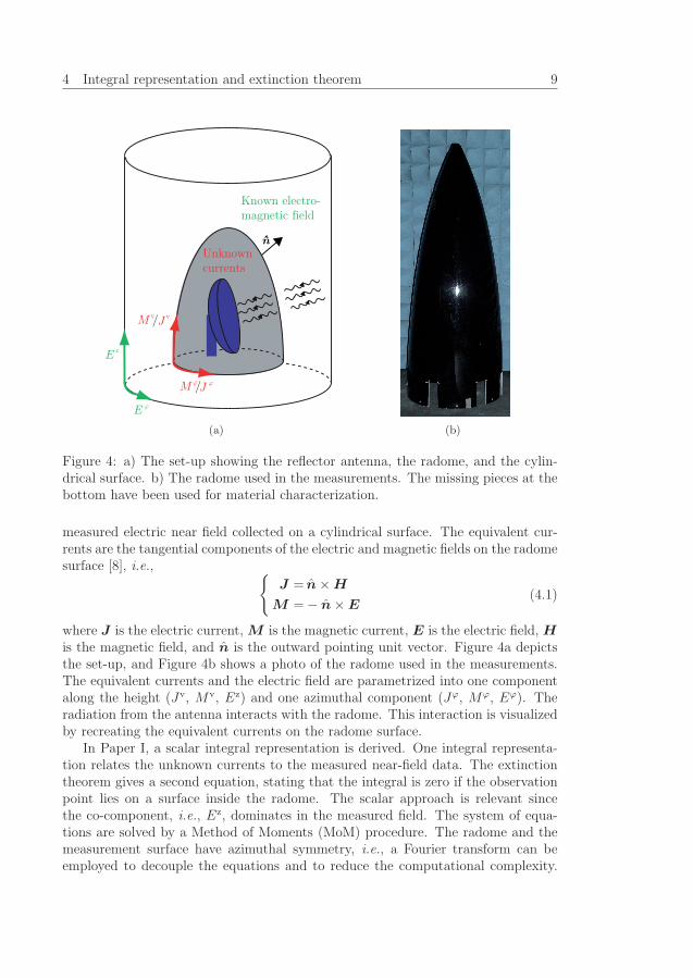
Figure 4: a) The set-up showing the reflector antenna, the radome, and the cylin-drical surface. b) The radome used in the measurements. The missing pieces at thebottom have been used for material characterization.

measured electric near field collected on a cylindrical surface. The equivalent cur-rents are the tangential components of the electric and magnetic fields on the radomesurface [8], i.e., {

J = n × H

M = − n × E(4.1)

where J is the electric current, M is the magnetic current, E is the electric field, His the magnetic field, and n is the outward pointing unit vector. Figure 4a depictsthe set-up, and Figure 4b shows a photo of the radome used in the measurements.The equivalent currents and the electric field are parametrized into one componentalong the height (Jv, Mv, Ez) and one azimuthal component (Jϕ, Mϕ, Eϕ). Theradiation from the antenna interacts with the radome. This interaction is visualizedby recreating the equivalent currents on the radome surface.

In Paper I, a scalar integral representation is derived. One integral representa-tion relates the unknown currents to the measured near-field data. The extinctiontheorem gives a second equation, stating that the integral is zero if the observationpoint lies on a surface inside the radome. The scalar approach is relevant sincethe co-component, i.e., Ez, dominates in the measured field. The system of equa-tions are solved by a Method of Moments (MoM) procedure. The radome and themeasurement surface have azimuthal symmetry, i.e., a Fourier transform can beemployed to decouple the equations and to reduce the computational complexity.


A singular value decomposition (SVD) is used to invert and regularize the matrix,i.e., remove singular values below a cut off level. The code is verified by using syn-thetic data, where the error is shown to be below −60 dB. Measured near-field data,originating from a reflector antenna, and collected on a cylindrical surface is theninvestigated. Three different configurations are studied, one with just the antenna,one with a radome enclosing the antenna, and finally one where a defect radome isplaced over the antenna. The amplitude of the reconstructed currents are visualizedin the frequency range 8 − 12 GHz, revealing diffraction effects. Introduced defectson the radome, i.e., copper plates, not visible in the near field data are localized inthe equivalent currents. The results are verified by calculating the far field from thereconstructed currents. This far-field pattern agrees very well with measurements.

The aim in Paper II is to obtain the phase of the reconstructed currents, e.g.,the insertion phase delay (IPD). The phase of the recreated currents is visualizedand analyzed in the frequency range 8 − 12 GHz. The thickness of the radome wallis approximated in order to validate the calculated phase shift. Different ways ofvisualizing the amplitude and phase of the equivalent currents are also discussedand presented in order to show which knowledge that can be extracted from themeasured near field.

In Paper III the analysis is derived for the full-wave electric field, i.e., the crosscomponent are no longer assumed to be negligible. The integral representation isevaluated at the radome surface instead of on a surface inside the radome whichgives a classical integral equation. That is, an integral equation that relates theunknown equivalent currents to each other on the radome surface, i.e.,

n(r) ×¨

Sradome

{jωμ0 g(r

′, r)J(r′) − j1

ωε0∇′g(r′, r)

[∇′S · J(r′)

]−∇′g(r′, r) × M(r′)

}dS ′ =

1

2M(r) r ∈ Sradome

where g(r′, r) is the free space Green’s function, n is the outward pointing normalof the radome surface, and ∇S is the surface divergence [15]. When necessary, theintegrals are interpreted as Cauchy’s principal value [15, 50]. The integral repre-sentation relates, as before, the equivalent currents to the measured near field, i.e.,

¨

Sradome

{−jωμ0 g(r

′, r)J(r′) + j1

ωε0∇′g(r′, r)

[∇′S · J(r′)

]+ ∇′g(r′, r) × M(r′)

}dS ′ = E(r) r outside Sradome

The approach of solution is the same as in Paper I-II. However, the expressions nowcontain coupled vector-valued fields and singular integrals. A detailed derivation ofthe representations is found in Appendix A.

The equivalent magnetic current is investigated at 8 GHz, see Figures 5 and 6.In Paper III the diffraction and transmission losses caused by the radome and the

5 General conclusions and future challenges 11

(a) (c)(b)-30

-20

-10

0

Figure 5: The recreated |Mϕ|-component on the front side of the radome. All valuesare normalized with the largest value of |Mϕ| when the defect radome is present andshown in dB-scale. (a) No radome present. (b) Radome present. (c) Defect radomepresent. The arrows point out the locations of the copper plates.

defect radome are depicted for both the co- and cross-polarized component. Alsoflash lobes caused by the radome are visualized. The effects of the defects, i.e.,copper plates, are localized in both the amplitude and phase components. However,to get the exact positions a combination of all components need to be analyzed. Theresults are verified by a comparison with the scalar code in Paper I. The resultsagree very well considering the cross-component is assumed to be zero in the scalarcode. The phase shift due to the radome, i.e., the IPD, is visualized and the resultsare promising which might lead to an alternative way of diagnosing radomes in thefuture.

5 General conclusions and future challenges

This thesis shows the potentials of the integral representation and the extinctiontheorem in solving the inverse source problem. In Paper I-II, the scalar represen-tation is explored. In Paper III, the vector-valued representation is investigatedby visualizing the reconstructed equivalent magnetic current on a radome surface.Future challenges are to analyze if also the electric equivalent current on the radomesurface can contribute to more knowledge. Moreover, investigation of the frequencydependence of the radome, using the full-wave representation, is planned. A closelyrelated question is the resolution of the equivalent currents. An initial investigationof this work is found in [45], where the problem is solved with spherical vector waves.


(a) (c)(b)-30

-20

-10

0

Figure 6: The recreated |Mv|-component on the front side of the radome. All valuesare normalized with the largest value of |Mv| when the defect radome is present andshown in dB-scale. (a) No radome present. (b) Radome present. (c) Defect radomepresent. The arrows point out the locations of the copper plates.

This paper gives a relation between the accuracy and resolution in the problem, andcalculates in which areas the solution is reliable.

The results reported in this thesis show great potential, and the method of cal-culating the IPD can hopefully be implemented for industrial use. Another excitingchallenge is to combine the method with the transmission of the field through theradome [4].

A Integral representations 13

n

nV

SS

Figure 7: The domain V of integration.

Appendix A Integral representations

There are several ways to derive the integral representations of the Maxwell equa-tions [15, 27, 43, 65]. In this appendix, one way is demonstrated [31].

The surface integral representation expresses the electromagnetic field in a ho-mogeneous and isotropic region in terms of its values on the bounding surface. Therepresentation states that if the electromagnetic field on a surface of a volume isknown, the electromagnetic field in the volume can be determined. The represen-tation is derived starting with two arbitrary scalar fields, φ(r) and ψ(r) and thedivergence relation

∇ · [φ(r)∇ψ(r) − ψ(r)∇φ(r)] = φ(r)∇2ψ(r) − ψ(r)∇2φ(r) (A.1)

The scalar fields are defined in a bounded domain V . The domain V is bounded bythe surface S with outward pointing normal vector n(r), see Figure 7. The surfacedoes not have to be a surface that separates two different materials, but can be anarbitrary surface in space.

Integration of (A.1) over the volume V and the use of the divergence theoremgive the Green’s second formula, i.e.,

¨

S

[φ(r)∇ψ(r) − ψ(r)∇φ(r)] · n(r) dS =

˚

V

[φ(r)∇2ψ(r) − ψ(r)∇2φ(r)

]dv

(A.2)Proceeding to the representation of vector fields, let the scalar field φ(r) in (A.2)

be [a ·F (r)], where a is an arbitrary constant vector and F (r) is a vector field. Wehave

¨

S

{[a · F (r)]∇ψ(r) − ψ(r)∇[a · F (r)]

}· n(r) dS

=

˚

V

{[a · F (r)]∇2ψ(r) − ψ(r)∇2[a · F (r)]

}dv


n

nV

SS

O

r

r

0

Figure 8: The domain V of integration. The variable of integration is denoted r′

and the observation point r.

Tedious algebra using differentiation rules of the Nabla-operator and the divergencetheorem give

¨

S

(ψ(r)

{n(r) × [∇× F (r)]

}+ ∇ψ(r)

[n(r) · F (r)

]− ψ(r)

[∇ · F (r)]n(r) −∇ψ(r) × [

n(r) × F (r)])

dS

=

˚

V

(F (r)∇2ψ(r) + ψ(r)

{∇× [∇× F (r)] −∇[∇ · F (r)]

})dv (A.3)

which is the Green’s vector formula. This equation is the foundation for findingintegral representations of vector fields.

A.1 Introduction of the scalar free space Green’s function

Let the scalar field ψ in (A.3) be the scalar Green’s function,

g(r, r′) =e−jk|r−r′|

4π|r − r′|using the time conventions ejωt. The variable of integration is denoted r′ and theobservation point r, see Figure 8. Assume r /∈ S. The Green’s function satisfies,

∇2g(r, r′) + k2g(r, r′) = 0 r′ �= r (A.4)


O

n

V -S

r

r

0

n

S

S

V"

"

º

Figure 9: The geometry for the evaluation of the limit process. The volume V ispunctuated by a ball of radius ε centered at the observation point r. The boundingsurface of this ball is Sε and its volume is denoted Vε. The variable of integration isdenoted r′.

where k is the wave number of the material. Replacing ψ in (A.3) with the scalarGreen’s function gives

¨

S

(g(r, r′)

{n(r′) × [∇′ × F (r′)

]}+ ∇′g(r, r′)

[n(r′) · F (r′)

]− g(r, r′)

[∇′ · F (r′)]n(r′) −∇′g(r, r′) × [

n(r′) × F (r′)])

dS ′

=

˚

V

(g(r, r′)

{∇′ × [∇′ × F (r′)

]−∇′[∇′ · F (r′)]− k2F (r′)

})dv′ (A.5)

where (A.4) is used. The Green’s function is singular at the point r′ = r. That is,the representation (A.5) is only valid when r′ �= r. The singularity can be treated inseveral ways. Here, the integrals are investigated in the limit of classical integrals.That is, a small ball Vε, centered at the singularity r, is excluded. The radius ofthis ball is ε and its spherical bounding surface is denoted Sε, see Figure 9. Lettingthe radius of the sphere approach zero, in (A.5), gives¨

S

... dS ′ + limr′→r

¨

Sε

... dS ′ =

˚

V

... dv′ − limr′→r

˚

Vε

... dv′ (A.6)

The surface Sε is parameterized in spherical coordinates, i.e., ε � 0, 0 � ϕ � 2π,and 0 � θ � π, with ez as the symmetry axis. The used notation is, cf., Figure 10,

ε = |r′ − r| dS = ε2 sin θ dϕ dθ

n = −ν dv = ε2 sin θ dε dϕ dθ(A.7)


O

V

r

r

0

S º"

" μ

"

ez

Figure 10: The geometry for the evaluation of integrals over the sphere Sε.

ν =r′ − r

ε= cosϕ sin θ ex + sinϕ sin θ ey + cos θ ez

∇′g(r, r′) =(r − r′) e−jk|r−r′|

4π|r − r′|3[1 + jk|r − r′|] = n

e−jkε

4πε

[1

ε+ jk

] (A.8)

where e denotes the Cartesian orthonormal basis vectors in the x-, y-, and z-direction, respectively.

In the integrals over the small sphere Sε, the normal unit vector ν varies rapidlyover the integral domain while the fields F , [∇ · F ], [∇× F ], {∇ × [∇× F

]}, and{∇[∇·F ]} are assumed to vary more slowly. Provided these fields are smooth (e.g.,Holder continuous), the mean value theorem for integrals implies that in the limitof ε→ 0 the fields can be evaluated at the singular point r [15]. Letting ε→ 0, i.e.,r′ → r, results in the following limits for the different parts in (A.5).

limε→0

¨

Sε

g(r, r′){

n(r′) × [∇′ × F (r′)]}

dS ′

= limε→0

¨

Sε

e−jkε

4πε

{n(r′) × [∇′ × F (r′)

]}ε2 sin θ′ dϕ′ dθ′ = 0

limε→0

¨

Sε

∇′g(r, r′)[n(r′) · F (r′)

]dS ′

= limε→0

¨

Sε

n(r′)e−jkε

4πε

[1

ε+ jk

] [n(r′) · F (r′)

]ε2 sin θ′ dϕ′ dθ′

=1

4π

¨

Sε

n(r′)[n(r′) · F (r)

]sin θ′ dϕ′ dθ′


=1

4π

πˆ

θ′=0

2πˆ

ϕ′=0

{[cosϕ′ sin θ′ ex + sinϕ′ sin θ′ ey + cos θ′ ez

]· [Fx(r) cosϕ′ sin θ′ + Fy(r) sinϕ′ sin θ′ + Fz(r) cos θ′

]sin θ′

}dϕ′ dθ′

=1

4π

[4π

3Fx(r) ex +

4π

3Fy(r) ey +

4π

3Fz(r) ez

]=

1

3F (r)

limε→0

¨

Sε

g(r, r′)[∇′ · F (r′)

]n(r′) dS ′

= limε→0

¨

Sε

e−jkε

4πε

[∇′ · F (r′)]n(r′) ε2 sin θ′ dϕ′ dθ′ = 0

limε→0

¨

Sε

∇′g(r, r′) × [n(r′) × F (r′)

]dS ′

= limε→0

¨

Sε

n(r′)e−jkε

4πε

[1

ε+ jk

]× [

n(r′) × F (r′)]ε2 sin θ′ dϕ′ dθ′

=1

4π

¨

Sε

n(r′) × [n(r′) × F (r)


=1

4π

¨

Sε

{n(r′)

[n(r′) · F (r)

]− F (r)[n(r′) · n(r′)

]}sin θ′ dϕ′ dθ′

=1

4π

[4π

3F (r) − 4πF (r)

]= −2

3F (r)

limε→0

˚

Vε

g(r, r′){∇′ × [∇′ × F (r′)

]−∇′[∇′ · F (r′)]− k2F (r′)

}dv′

= limε→0

˚

Vε

e−jkε

4πε

{∇′ × [∇′ × F (r′)

]−∇′[∇′ · F (r′)]

− k2F (r′)}ε2 sin θ′ dε dϕ′ dθ′ = 0

The parts are inserted into (A.6) giving

¨

S

... dS ′ + F (r) =

˚

V

... dv′ − 0 r ∈ V


Including the region without singularities, i.e., r /∈ V , from (A.5), gives

˚

V

(g(r, r′)

{∇′ × [∇′ × F (r′)

]−∇′[∇′ · F (r′)]− k2F (r′)

})dv′

−¨

S

(g(r, r′)

{n(r′) × [∇′ × F (r′)

]}+ ∇′g(r, r′)

[n(r′) · F (r′)

]− g(r, r′)

[∇′ · F (r′)]n(r′) −∇′g(r, r′) × [

n(r′) × F (r′)])

dS ′

=

{F (r) r ∈ V

0 r /∈ V

(A.9)

This is a general representation of a vector field F . The field F is represented asa volume integral of its values in V and as a surface integral of its values over thebounding surface S of V . If these integrals are evaluated at a point r that liesoutside the volume V , these integrals cancel each other — the extinction theorem.It is important to notice that this does not necessarily mean that the field F isidentically zero outside the volume V — only the values of the integrals cancel.

A.2 Introduction of the Maxwell equations

So far, the vector field F has been an arbitrary vector field. This field can be chosenas the electric or magnetic field that satisfies the source free Maxwell equations withthe time convention ejωt, i.e., {

∇× E = −jωB

∇× H = jωD(A.10)

The constitutive relations in a homogeneous, isotropic region are given by{D = ε0εE

B = μ0μH(A.11)

Combination of (A.10) and (A.11) give{∇× E = −jωμ0μH

∇× H = jωε0εE(A.12)

{∇× (∇× E) = k2E

∇× (∇× H) = k2H(A.13)

{∇ · E = 0

∇ · H = 0(A.14)


where ε0 is the permittivity of vacuum, ε the relative permittivity, μ0 the per-meability of vacuum, μ the relative permeability, ω the angular frequency, andk = ω

√ε0μ0εμ the wave number.

Letting F be the electric field E in (A.9) gives together with (A.12)-(A.14) asurface integral representation for the electric field, i.e.,

¨

S

{jωμ0μ g(r, r

′)[n(r′) × H(r′)

]−∇′g(r, r′)[n(r′) · E(r′)

]+ ∇′g(r, r′) × [

n(r′) × E(r′)]}

dS ′ =

{E(r) r inside S

0 r outside S(A.15)

where the surface S is shown in Figure 8. Observe that the volume integral iszero and only the surface integral remains. The relative permittivity ε and therelative permeability μ may depend on the angular frequency ω, i.e., the materialcan be dispersive, but constant as a function of space (homogeneous material). IfF is interchanged by the magnetic field H , a surface integral representation forthe magnetic field is attained. The integral representation (A.15) contains both thenormal and the tangential components of the electromagnetic field. In practice, itis more convenient to work only with the tangential fields. The normal component,i.e., the second term in (A.15), can be written in terms of a tangential componentby an application of the Maxwell equations (A.10)-(A.11), i.e.,

n(r) · E(r) = −j1

ωε0εn(r) · [∇× H(r)

]= j

1

ωε0ε∇S · [n(r) × H(r)

]where the identity ∇S · (n × a) = −n · (∇×a) is used with a denoting an arbitraryvector and ∇S· the surface divergence [15]. That gives a surface integral represen-tation for the electric field consisting of only tangential components on the surfaceS, i.e.,

¨

S

(jωμ0μ g(r, r

′)[n(r′) × H(r′)

]− j1

ωε0ε∇′g(r, r′)

{∇′

S · [n(r′) × H(r′)]}

+ ∇′g(r, r′) × [n(r′) × E(r′)

])dS ′ =

{E(r) r inside S

0 r outside S(A.16)

A.3 Values of the integral equations on the surface S

The integral representation in (A.16) is defined for all r /∈ S. To include the surfaceinto the domain it must be studied what happens as r approaches S. At this stageit is not even clear that these limit values exist at all. The integrands in (A.16)become singular as r moves toward the surface. This singularity can be treated inseveral ways. Here, a classic approach is used, where the limit is investigated byadding a half sphere from the outside and the inside, respectively.


O

V

S

r

r

0

n

S

"

º

(a) (b)

O

S"

punc

puncμ

"

ez

rr0

Figure 11: (a) The geometry for the evaluation of the limit process. In the limit thesurface (S ′ = Spunc ∪ Sε) → S and Vpunc → V . (b) The parameterization of the halfsphere Sε. Observe that n = −ν.

Starting with the approach from the outside, the integral representation is,see (A.16)

¨

S

(jωμ0μ g(r, r

′)[n(r′) × H(r′)

]− j1


{∇′

S · [n(r′) × H(r′)]}

+ ∇′g(r, r′) × [n(r′) × E(r′)

])dS ′ = 0 r /∈ V

It is applied to a volume Vpunc which is slightly deformed compared to the originalvolume V , i.e., a small half ball of radius ε is excluded. The bounding surface of thevolume Vpunc is denoted S ′ and consists of two parts: the punctuated surface Spunc,and a half sphere Sε of radius ε, i.e., S ′ = Spunc ∪ Sε, see Figure 11a. In the limitε→ 0 the surface S ′ → S and Vpunc → V , i.e.,

limr′→r

¨

S′

... dS ′ =

S

... dS ′ + limr′→r

¨

Sε

... dS ′ (A.17)

where the integralfflffl... dS denotes Cauchy’s principal value [50].

To investigate the limit of the integral over the surface Sε, this surface is param-eterized by the spherical angles 0 � ϕ � 2π and 0 � θ � π/2 with the direction ez

as the symmetry axis, see Figure 11b and (A.7)-(A.8). The normal unit vector νvaries rapidly over the small half sphere Sε, while the electromagnetic fields E andH are assumed to vary more slowly. Provided these fields are smooth (e.g., Holdercontinuous), the mean value theorem for integrals implies that in the limit of ε→ 0the fields can be evaluated at the point r [15]. Letting ε → 0, in the integrals over


Sε, give the following limits1

limε→0

¨

Sε

g(r, r′)[n(r′) × H(r′)

]dS ′

= limε→0

¨

Sε

e−jkε

4πε

[−ν(r′) × H(r′)]ε2 sin θ′ dϕ′ dθ′ = 0

limε→0

¨

Sε

− j1

ωε0εr∇′g(r, r′)

{∇′

S · [n(r′) × H(r′)]}

dS ′

= limε→0

¨

Sε

−∇′g(r, r′)[n(r′) · E(r′)

]dS ′

= limε→0

¨

Sε

ν(r′)e−jkε

4πε

[1

ε+ jk

] [−ν(r′) · E(r′)]ε2 sin θ′ dϕ′ dθ′

= − 1

4π

¨

Sε

ν(r′)[ν(r′) · E(r)


= − 1

4π

π/2ˆ

θ′=0

2πˆ

ϕ′=0

{[cosϕ′ sin θ′ ex + sinϕ′ sin θ′ ey + cos θ′ ez

]· [Ex(r) cosϕ′ sin θ′ + Ey(r) sinϕ′ sin θ′ + Ez(r) cos θ′

]sin θ′

}dϕ′ dθ′

= − 1

4π

[2π

3Ex(r) ex +

2π

3Ey(r) ey +

2π

3Ez(r) ez

]= −1

6E(r)

limε→0

¨

Sε

∇′g(r, r′) × [n(r′) × E(r′)

]dS ′

= limε→0

¨

Sε

−ν(r′)e−jkε

4πε

[1

ε+ jk

]× [−ν(r′) × E(r′)

]ε2 sin θ′ dϕ′ dθ′

=1

4π

¨

Sε

ν(r′) × [ν(r′) × E(r)


=1

4π

π/2ˆ

θ′=0

2πˆ

ϕ′=0

{ν(r′)

[ν(r′) · E(r)

]− E(r)[ν(r′) · ν(r′)

]}sin θ′ dϕ′ dθ′

=1

4π

[2π

3E(r) − 2πE(r)

]= −1

3E(r)

The limit values above are plugged into (A.17), i.e.,

1In the second integral, the relative permittivity is temporarily denoted by εr to avoid mix upwith the radius ε.


O

V

Sr

r

0

n

S "

º

(a) (b)

O

S"

punc

puncμ

"

ez

r

r0

Figure 12: (a) The geometry for the evaluation of the limit process. In the limit thesurface (S ′ = Spunc ∪ Sε) → S and Vpunc → V . (b) The parameterization of the halfsphere Sε. Observe that now n = ν.

S

(jωμ0μ g(r, r

′)[n(r′) × H(r′)

]− j1


{∇′

S · [n(r′) × H(r′)]}

+ ∇′g(r, r′) × [n(r′) × E(r′)

])dS ′ =

1

2E(r) r ∈ S (A.18)

which is the limit value of the surface integral representation for the electric fieldwhen approaching from the outside.2

If the limit is taken from the inside instead, the integral representation, (A.16),i.e.,

¨

S

(jωμ0μ g(r, r

′)[n(r′) × H(r′)

]− j1

ωε0εr∇′g(r, r′)

{∇′

S · [n(r′) × H(r′)]}

+ ∇′g(r, r′) × [n(r′) × E(r′)

])dS ′ = E(r) r ∈ V (A.19)

is applied to a volume Vpunc shown in Figure 12a. The derivation is similar to theanalysis above. The difference is that now n = ν. This changes the sign in thelimit processes, which inserted in (A.19) give the same final integral equation, i.e.,(A.18).

The representation (A.18) consists of three components, two describing the tan-gential field and one describing the normal component of the field. Since the normalcomponent can be determined by the knowledge of the tangential parts the normal

2The first surface integral does not have to be written as Cauchy’s principle value sincefflfflS

. . . dS =˜S

. . . dS.


S

r

r

n º

n

rS

(a) (b)

0r0

O O

Figure 13: (a) The interior problem. (b) The exterior problem.

component can be eliminated [43], i.e.,

n(r)×

S

(jωμ0μ g(r, r

′)[n(r′)×H(r′)

]−j1


{∇′

S ·[n(r′)×H(r′)

]}+ ∇′g(r, r′) × [

n(r′) × E(r′)])

dS ′ =1

2n(r) × E(r) r ∈ S (A.20)

A.4 The equivalent surface currents

The electric and magnetic equivalent surface currents, J and M , are defined as [8]{J(r) = n(r) × H(r)

M(r) = − n(r) × E(r)

Introducing the equivalent currents in (A.16) and (A.20) yield a surface integralrepresentation and a surface integral equation for the electric field⎧⎪⎪⎪⎪⎪⎪⎪⎪⎪⎪⎪⎪⎨⎪⎪⎪⎪⎪⎪⎪⎪⎪⎪⎪⎪⎩

¨

S

{jωμ0μ g(r, r

′)J(r′) − j1


[∇′S · J(r′)

]−∇′g(r, r′) × M(r′)

}dS ′ = E(r) r inside S

n(r) ×

S

{jωμ0μ g(r, r

′)J(r′) − j1


[∇′S · J(r′)

]−∇′g(r, r′) × M(r′)

}dS ′ = −1

2M(r) r ∈ S

The regions are depicted in Figure 13a.In this thesis, the integral representation and equation are applied to the exterior

problem, i.e., see Figure 13b. This volume is not bounded. However, employing the


Silver-Muller radiation conditions, the solution of the Maxwell equations satisfiesthe following integral representation [29, 43, 60, 65]⎧⎪⎪⎪⎪⎪⎪⎪⎪⎪⎪⎪⎪⎨⎪⎪⎪⎪⎪⎪⎪⎪⎪⎪⎪⎪⎩

¨

S

{jωμ0μ g(r, r

′)J(r′) − j1


[∇′S · J(r′)

]−∇′g(r, r′) × M(r′)

}dS ′ = −E(r) r outside S

ν(r) ×

S

{jωμ0μ g(r, r

′)J(r′) − j1


[∇′S · J(r′)

]−∇′g(r, r′) × M(r′)

}dS ′ =

1

2M(r) r ∈ S

where the change of signs is due to the choice of normal, i.e., ν = −n.

References

[1] Y. Alvarez and F. Las-Heras. Integral equation algorithms for equivalent cur-rents distribution retrieval over arbitrary three-dimensional surfaces. In Proc.2006 IEEE Antennas and Propagation Society International Symp., pages 1061–1064, Albuquerque, New Mexico, 2006.

[2] Y. Alvarez, F. Las-Heras, and M. R. Pino. Full-wave method for RF sourceslocation. In Proc. Second European Conference on Antennas and Propagation,pages 1–5, Edinburgh, UK, 2007. The Institution of Engineering and Technol-ogy.

[3] Y. Alvarez, F. Las-Heras, and M. R. Pino. Reconstruction of equivalent cur-rents distribution over arbitrary three-dimensional surfaces based on integralequation algorithms. IEEE Trans. Antennas Propagat., 55(12), 3460–3468,2007.

[4] M. Andersson. Software for analysis of radome performance. In Proc. Interna-tional Conference on Electromagnetics in Advanced Applications (ICEAA’05),pages 537–539, Torino, Italy, 2005.

[5] B. Audone, A. Delogu, and P. Moriondo. Radome design and measurements.IEEE Trans. Antennas Propagat., 37(2), 292–295, 1988.

[6] R. G. Ayestaran and F. Las-Heras. Near field to far field transformation us-ing neural networks and source reconstruction. J. Electromagn. Waves Appl.,20(15), 2201–2213, 2006.

[7] R. G. Ayestaran and F. Las-Heras. Neural network-based array synthesis inpresence of obstacles. International Journal of Numerical Modelling-ElectronicNetworks Devices and Fields, 19, 1–13, 2006.

References 25

[8] C. A. Balanis. Advanced Engineering Electromagnetics. John Wiley & Sons,New York, 1989.

[9] A. Bondeson, T. Rylander, and P. Ingelstrom. Computational Electromagnetics.Springer-Verlag, Berlin, 2005.

[10] H. G. Booker and P. C. Clemmow. The concept of an angular spectrum ofplane waves and its relation to that of polar diagram and aperture distribution.Proc. Inst. Elec. Eng., 97(1), 11–16, 1950.

[11] A. Bostrom, G. Kristensson, and S. Strom. Transformation properties of plane,spherical and cylindrical scalar and vector wave functions. In V. V. Varadan,A. Lakhtakia, and V. K. Varadan, editors, Field Representations and Intro-duction to Scattering, Acoustic, Electromagnetic and Elastic Wave Scattering,chapter 4, pages 165–210. Elsevier Science Publishers, Amsterdam, 1991.

[12] O. M. Bucci, M. D. Migliore, G. Panariello, and P. Sgambato. Accurate diag-nosis of conformal arrays from near-field data using the matrix method. IEEETrans. Antennas Propagat., 53(3), 1114–1120, 2005.

[13] C. Cappellin, O. Breinbjerg, and A. Frandsen. Properties of the transformationfrom the spherical wave expansion to the plane wave expansion. Radio Sci.,43(1), 2008.

[14] C. Cappellin, A. Frandsen, and O. Breinbjerg. Application of the SWE-to-PWEantenna diagnostics technique to an offset reflector antenna. IEEE Antennasand Propagation Magazine, 50(5), 204–213, 2008.

[15] D. Colton and R. Kress. Integral Equation Methods in Scattering Theory. JohnWiley & Sons, New York, 1983.

[16] L. E. Corey and E. B. Joy. On computation of electromagnetic fields on pla-nar surfaces from fields specified on nearby surfaces. IEEE Trans. AntennasPropagat., 29(2), 402–404, 1981.

[17] A. Delogu and M. Mwanya. Design and testing of a radome for a beam steer-ing radar antenna. In Proc. International Conference on Electromagnetics inAdvanced Applications (ICEAA’05), pages 505–508, Torino, Italy, 2005.

[18] A. J. Devaney and E. Wolf. Radiating and nonradiating classical current dis-tributions and the fields they generate. Phys. Rev. D, 8(4), 1044–1047, 1973.

[19] A. J. Devaney and E. Wolf. Multipole expansions and plane wave representa-tions of the electromagnetic field. J. Math. Phys., 15(2), 234–244, 1974.

[20] T. F. Eibert and C. H. Schmidt. Multilevel fast multipole accelerated inverseequivalent current method employing Rao-Wilton-Glisson discretization of elec-tric and magnetic surface currents. IEEE Trans. Antennas Propagat., 57(4),1178–1185, 2009.


[21] J. Friden, H. Isaksson, B. Hansson, and B. Thors. Robust phase-retrieval forquick whole-body SAR assessment using dual plane amplitude-only data. Elec-tronics Letters, 45(23), 1155–1157, 2009.

[22] M. G. Guler and E. B. Joy. High resolution spherical microwave holography.IEEE Trans. Antennas Propagat., 43(5), 464–472, 1995.

[23] J. Hanfling, G. Borgiotti, and L. Kaplan. The backward transform of the nearfield for reconstruction of aperture fields. IEEE Antennas and PropagationSociety International Symposium, 17, 764–767, 1979.

[24] J. E. Hansen, editor. Spherical Near-Field Antenna Measurements. Number 26in IEE electromagnetic waves series. Peter Peregrinus Ltd., Stevenage, UK,1988. ISBN: 0-86341-110-X.

[25] T. B. Hansen and A. D. Yaghjian, editors. Plane-wave theory of time-domainfields: near-field scanning applications. IEEE electromagnetic wave theory.IEEE Press, New York, 1999. ISBN: 0-7803-3428-0.

[26] M. M. Hernando, A. Fernandez, M. Arias, M. Rodriguez, Y. Alvarez, andF. Las-Heras. EMI radiated noise measurement system using the source re-construction technique. IEEE Trans. Industrial Electronics, 55(9), 3258–3265,2008.

[27] D. S. Jones. Acoustic and Electromagnetic Waves. Oxford University Press,New York, 1986.

[28] S. M. Kay. Fundamentals of Statistical Signal Processing, Estimation Theory.Prentice-Hall, Inc., NJ, 1993.

[29] R. E. Kleinman and G. F. Roach. Boundary integral equations for the three-dimensional Helmholtz equation. SIAM Review, 16(2), 214–236, 1974.

[30] B. M. Kolundzija and A. R. Djordjevic. Electromagnetic modeling of compositemetallic and dielectric structures. Artech House, Boston, London, 2002.

[31] G. Kristensson. Spridningsteori med antenntillampningar. Studentlitteratur,Lund, 1999. (In Swedish).

[32] F. Las-Heras, B. Galocha, and Y. Alvarez. On the sources reconstructionmethod application for array and aperture antennas diagnostics. MicrowaveOpt. Techn. Lett., 51(7), 1664–1668, 2009.

[33] F. Las-Heras, B. Galocha, and J. L. Besada. Far-field performance of linearantennas determined from near-field data. IEEE Trans. Antennas Propagat.,50(3), 408–410, 2002.

[34] F. Las-Heras, M. R. Pino, S. Loredo, Y. Alvarez, and T. K. Sarkar. Evaluatingnear-field radiation patterns of commercial antennas. IEEE Trans. AntennasPropagat., 54(8), 2198–2207, 2006.

References 27

[35] F. Las-Heras and T. K. Sarkar. Radial field retrieval in spherical scanningfor current reconstruction and NF–FF transformation. IEEE Trans. AntennasPropagat., 50(6), 866–874, 2002.

[36] J.-J. Laurin, J.-F. Zurcher, and F. E. Gardiol. Near-field diagnostics of smallprinted antennas using the equivalent magnetic current approach. IEEE Trans.Antennas Propagat., 49(5), 814–828, 2001.

[37] J. Lee, E. M. Ferren, D. P. Woollen, and K. M. Lee. Near-field probe used as adiagnostic tool to locate defective elements in an array antenna. IEEE Trans.Antennas Propagat., 36(6), 884–889, 1988.

[38] I. V. Lindell. Methods for Electromagnetic Field Analysis. IEEE Press andOxford University Press, Oxford, 1995.

[39] C.-C. Lu. A fast algorithm based on volume integral equation for analysis ofarbitrary shaped dielectric radomes. IEEE Trans. Antennas Propagat., 51(3),606–612, 2003.

[40] E. A. Marengo and A. J. Devaney. The inverse source problem of electro-magnetics: Linear inversion formulation and minimum energy solution. IEEETrans. Antennas Propagat., 47(2), 410–412, February 1999.

[41] E. A. Marengo, A. J. Devaney, and F. K. Gruber. Inverse source problem withreactive power constraint. IEEE Trans. Antennas Propagat., 52(6), 1586–1595,June 2004.

[42] E. A. Marengo and R. W. Ziolkowski. Nonradiating and minimum energysources and their fields: Generalized source inversion theory and applications.IEEE Trans. Antennas Propagat., 48(10), 1553–1562, October 2000.

[43] C. Muller. Foundations of the Mathematical Theory of Electromagnetic Waves.Springer-Verlag, Berlin, 1969.

[44] M. S. Narasimhan and B. P. Kumar. A technique of synthesizing the excitationcurrents of planar arrays or apertures. IEEE Trans. Antennas Propagat., 38(9),1326–1332, 1990.

[45] S. Nordebo, M. Gustafsson, and K. Persson. Sensitivity analysis for antennanear-field imaging. IEEE Trans. Signal Process., 55(1), 94–101, January 2007.

[46] S. Nordebo and M. Gustafsson. Statistical signal analysis for the inverse sourceproblem of electromagnetics. IEEE Trans. Signal Process., 54(6), 2357–2361,June 2006.

[47] A. F. Peterson, S. L. Ray, and R. Mittra. Computational Methods for Electro-magnetics. IEEE Press, New York, 1998.


[48] P. Petre and T. K. Sarkar. Planar near-field to far-field transformation usingan equivalent magnetic current approach. IEEE Trans. Antennas Propagat.,40(11), 1348–1356, 1992.

[49] P. Petre and T. K. Sarkar. Planar near-field to far-field transformation usingan array of dipole probes. IEEE Trans. Antennas Propagat., 42(4), 534–537,1994.

[50] A. J. Poggio and E. K. Miller. Integral equation solutions of three-dimensionalscattering problems. In R. Mittra, editor, Computer Techniques for Electro-magnetics. Pergamon, New York, 1973.

[51] S. Poulsen. Stealth radomes. PhD thesis, Lund University, Department ofElectroscience, Lund University, P.O. Box 118, S-221 00 Lund, Sweden, 2006.

[52] D. M. Pozar. Microwave Engineering. John Wiley & Sons, New York, 1998.

[53] Y. Rahmat-Samii. Surface diagnosis of large reflector antennas using microwaveholographic metrology: an iterative approach. Radio Sci., 19(5), 1205–1217,1984.

[54] Y. Rahmat-Samii and J. Lemanczyk. Application of spherical near-field mea-surements to microwave holographic diagnosis of antennas. IEEE Trans. An-tennas Propagat., 36(6), 869–878, 1988.

[55] D. J. Rochblatt and B. L. Seidel. Microwave antenna holography. IEEE Trans.Microwave Theory Tech., 40(6), 1294–1300, 1992.

[56] T. K. Sarkar and A. Taaghol. Near-field to near/far-field transformation forarbitrary near-field geometry utilizing an equivalent electric current and MoM.IEEE Trans. Antennas Propagat., 47(3), 566–573, March 1999.

[57] J. A. Shifflett. CADDRAD: A physical opics radar/radome analysis code forarbitrary 3D geometries. IEEE Antennas and Propagation Magazine, 6(39),73–79, 1997.

[58] R. A. Shore and A. D. Yaghjian. Dual surface electric field integral equation.Air Force Research Laboratory Report, 2001. No. AFRL-SN-HS-TR-2001-013.

[59] R. A. Shore and A. D. Yaghjian. Dual-surface integral equations in electromag-netic scattering. IEEE Trans. Antennas Propagat., 53(5), 1706–1709, 2005.

[60] S. Silver. Microwave Antenna Theory and Design, volume 12 of RadiationLaboratory Series. McGraw-Hill, New York, 1949.

[61] J. C.-E. Sten. Reconstruction of electromagnetic minimum energy sources in aprolate spheroid. Radio Sci., 39(2), 2004.

[62] J. C.-E. Sten and E. A. Marengo. Inverse source problem in an oblate spheroidalgeometry. IEEE Trans. Antennas Propagat., 54(11), 3418–3428, 2006.

References 29

[63] J. C.-E. Sten and E. A. Marengo. Inverse source problem in the spheroidalgeometry: Vector formulation. IEEE Trans. Antennas Propagat., 56(4), 961–969, 2008.

[64] W. R. Stone. A review and examination of results on uniqueness in inverseproblems. Radio Sci., 22(6), 1026–1030, November 1987.

[65] S. Strom. Introduction to integral representations and integral equations fortime-harmonic acoustic, electromagnetic and elastodynamic wave fields. InV. V. Varadan, A. Lakhtakia, and V. K. Varadan, editors, Field Representationsand Introduction to Scattering, volume 1 of Handbook on Acoustic, Electromag-netic and Elastic Wave Scattering, chapter 2, pages 37–141. Elsevier SciencePublishers, Amsterdam, 1991.

[66] A. Taaghol and T. K. Sarkar. Near-field to near/far-field transformation forarbitrary near-field geometry, utilizing an equivalent magnetic current. IEEETrans. Electromagn. Compatibility, 38(3), 536–542, 1996.

[67] F. Therond, J. C. Bolomey, N. Joachmowicz, and F. Lucas. Electromagneticdiagnosis technique using spherical near-field probing. In Proc. EUROEM’94,pages 1218–1226, Bordeaux, France, 1994.

[68] A. R. Tobin, A. D. Yaghjian, and M. M. Bell. Surface integral equation formulti-wavelength, arbitrarily shaped, perfectly conducting bodies. In Digest ofthe National Radio Science Meeting (URSI), page 9, Boulder, Colorado, 1987.

[69] J. G. van Bladel. Electromagnetic Fields. IEEE Press, New York, 2007.

[70] V. V. Varadan and V. K. Varadan. Acoustic, electromagnetic and elastodynam-ics fields. In V. V. Varadan, A. Lakhtakia, and V. K. Varadan, editors, FieldRepresentations and Introduction to Scattering, Acoustic, Electromagnetic andElastic Wave Scattering, chapter 1, pages 1–35. Elsevier Science Publishers,Amsterdam, 1991.

[71] J. J. H. Wang. An examination of the theory and practices of planar near-fieldmeasurement. IEEE Trans. Antennas Propagat., 36(6), 746–753, 1988.

[72] M. B. Woodworth and A. D. Yaghjian. Derivation, application and conjugategradient solution of dual-surface integral equations for three-dimensional, multi-wavelength perfect conductors. Progress in Electromagnetics Research, 5, 103–129, 1991.

[73] M. B. Woodworth and A. D. Yaghjian. Multiwavelength three-dimensionalscattering with dual-surface integral equations. J. Opt. Soc. Am. A, 11(4),1399–1413, 1994.

[74] R. G. Yaccarino and Y. Rahmat-Samii. Phaseless bi-polar planar near-fieldmeasurements and diagnostics of array antennas. IEEE Trans. Antennas Prop-agat., 47(3), 574–583, 1999.


[75] W.-J. Zhao, L.-W. Li, and Y.-B. Gan. Efficient analysis of antenna radiationin the presence of airborne dielectric radomes of arbitrary shape. IEEE Trans.Antennas Propagat., 53(1), 442–449, 2005.

[76] A. Ziyyat, L. Casavola, D. Picard, and J. C. Bolomey. Prediction of BTSantennas safety perimeter from NF to NF transformation: an experimentalvalidation. In Proc. Antenna Measurement Techniques Association (AMTA),pages 22–26, Denver, US, 2001.

Paper I

Reconstruction ofequivalent currents using anear-field datatransformation – withradome applications

Kristin Persson and Mats Gustafsson

Based on: K. Persson and M. Gustafsson. Reconstruction of equivalent currentsusing a near-field data transformation – with radome applications, Progress in Elec-tromagnetics Research, vol. 54, pp. 179–198, 2005.

1 Introduction 33

Abstract

Knowledge of the current distribution on a radome can be used to improveradome design, detect manufacturing errors, and to verify numerical simula-tions. In this paper, the transformation from near-field data to its equivalentcurrent distribution on a surface of arbitrary material, i.e., the radome, isanalyzed. The transformation is based on the scalar surface integral represen-tation that relates the equivalent currents to the near-field data. The presenceof axial symmetry enables usage of the fast Fourier transform (FFT) to reducethe computational complexity. Furthermore, the problem is regularized usingthe singular value decomposition (SVD). Both synthetic and measured dataare used to verify the method. The quantity of data is vast since the heightof the radome corresponds to 29 − 43 wavelengths in the frequency interval8.0 − 12.0 GHz. It is shown that the method gives an accurate descriptionof the field radiated from an antenna, on a surface enclosing it. Moreover,disturbances introduced by copper plates attached to the radome surface, notlocalized in the measured near field, are focused and detectable in the equiv-alent currents.

1 Introduction

There are several applications of a near field to equivalent currents transformation.For example, in the radome industry it is important to have accurate models of thefield radiated from the antenna inside the radome. This field cannot be measureddirectly since the radome often is placed very close to the antenna and at thesedistances, there is a substantial interaction between the antenna and the measuringprobe [5, 10, 16]. Another field of application is in the manufacturing of radiatingbodies, i.e., radomes, antenna arrays etc., when the radiation pattern from the bodydoes not exhibit the expected form. By determination of the equivalent currents onthe radiating body the malfunctioning areas or components can be found.

A common method, transforming near field to equivalent currents and vice versa,is to use modal-expansions of the electric field [5]. This is a very efficient method forradiating bodies with certain geometrical symmetries, i.e., planar, cylindrical, andspherical. Having a planar aperture the plane wave spectrum of the field is utilized inthe back transformation [3, 4]. The fact that the expression of the far field originatingfrom a planar surface is equal to the Fourier transform of the radiating field on theaperture has been investigated in [9, 10]. The paper [9] also illustrates that defects,i.e., patches of Eccosorb, can be detected on the aperture. If the radiating bodyis of cylindrical or spherical geometry the radial solutions contain cylindrical andspherical Bessel functions while the angular solutions are described by trigonometricfunctions and the associated Legendre functions, respectively [5, 14]. For generalgeometrical symmetries, where modal-expansions do not exist, the modal-expansionis not applicable.

Later on different combinations of the electric- and magnetic-field integral equa-tions (EFIE and MFIE) derived from the Maxwell equations, cf., the Method ofMoments (MoM), have been used to back propagate fields towards their origin, i.e.,

34 Paper I

a linear inverse source problem is solved. By this method it is possible to handle awider class of geometries [10]. In [15] the dual-surface magnetic and electric-field in-tegral equations are investigated. The fields are transformed back to a cubic perfectelectric conductor by solving the dual-surface magnetic-field integral equation usingthe conjugate gradient method. Other work using the integral equations is reportedin [11], where the near field is measured on a arbitrary surface and later invertedto a planar perfectly conducting surface by using a singular value decomposition(SVD) for regularization.

In this paper, the approach is to investigate a scalar surface integral representa-tion that does not require the aperture to be a perfect electric or magnetic conductor.The representation provides a relation relating the unknown electric and magneticequivalent currents on a surface to the measured electric field. An additional re-lation is given by the fact that the equivalent currents are constructed such thatthe integral is zero inside the volume, on which surface the currents exist, i.e., theextinction theorem [13].

The integral relations are discretized into matrix linear equations. The matrixequations include an azimuthal convolution which is solved with a fast Fourier trans-form (FFT) in the angular coordinate. The fast Fourier transform brings down thecomplexity of the problem, i.e., the original surface-to-surface linear map is decom-posed into a set of line-to-line linear maps. A singular value decomposition (SVD)is used to invert each of these linear maps. As most inverse problems it is ill-posed,i.e., small errors in the near-field data can produce large errors in the equivalentcurrents. Thus, the problem needs to be regularized by suppression of small singularvalues when inverted.

In this paper, the electric field to be inverted is presumed to be scalar, i.e., thescalar surface integral representation is utilized. The assumption is acceptable sincethe used near-field data, supplied by SAAB Bofors Dynamics and Chelton AppliedComposites, Sweden, clearly have one dominating component in the main lobe,see Figure 3. The measured data is given for three different antenna and radomeconfigurations, viz., antenna, antenna together with radome, and antenna togetherwith defect radome. The height of the radome corresponds to 29 − 43 wavelengthsin the frequency interval 8.0 − 12.0 GHz.

As a start, synthetic data is used to verify the method. Verification is alsoperformed by a comparison between the measured far field and the far field calculatedfrom the equivalent currents on the radome. The calculated far field agrees well withthe measured far field. We show that the method can describe the field radiatedfrom an antenna, on a surface enclosing it. When the radome is introduced thefield is scattered and flash lobes arise. The equivalent currents on the radome, thatproduce the electric field measured in the near-field area, are identified and the flashlobes are accurately detected.

Manufacturing errors, not localized in the measured near-field data, can be fo-cused and detected in the equivalent currents on the radome surface. In this paper,it is shown that the field scattered by copper plates attached on the radome, arefocused back towards the original position of the copper plates. The length of theside of the square copper plates is 6 cm, i.e., 1.6− 2.4 wavelengths corresponding to

2 Near-field measurements 35

Figure 1: Photo of the cylindrical near-field range at SAAB Bofors Dynamics,Sweden. The antenna under test is rotated and the probe is moved in the verticaldirection. A close up of the reflector antenna is shown in the upper right corner.

the frequency span 8.0 − 12.0 GHz.In Section 2 the experimental set-up is described and the measured near-field

data is presented. The scalar surface integral representation is introduced andadapted to the specific problem in Section 3. Section 4 discusses the implemen-tation process of the scalar surface integral representation. Results, using syntheticnear-field data and the error of the method is elucidated. The results, when usingthe experimental near-field data, are shown and examined in Section 5. The paperends with the achieved conclusions in Section 6.

2 Near-field measurements

The near-field data, used in this paper, was supplied by SAAB Bofors Dynamicsand Chelton Applied Composites, Sweden. The set-up with relevant dimensionsindicated is shown in Figures 1 and 2a. Three different measurements were per-formed; data measured without the radome, data measured with the radome, anddata measured with the defect radome. The defect radome has two copper platesattached to its surface.

A reflector antenna fed by a symmetrically placed wave-guide generates the near-field data, see Figure 1. The diameter of the antenna is 0.32 m and its focal distanceis 0.1 m. The main lobe of the antenna is vertically polarized relative to the hori-zontal plane. The standing wave ratio (SWR) is approximately 1.4 in the frequencyrange 8.2 − 9.5 GHz. The antenna is poorly adapted for other frequencies. A 10 dBreflection attenuator is connected to the antenna.

36 Paper I

a) b)

zizm

zp

ϕn

ϕj

ϕj

z/mm

800

342

0

-728-800

ρ/mm0 213 459

33

320

0 ≤ i ≤ Ni − 10 ≤ j ≤ Nj − 10 ≤ m ≤ Nm − 10 ≤ n ≤ Nn − 10 ≤ p ≤ Np − 1

Figure 2: (a) The dimensions of the reflector antenna, the radome, and the cylinderwhere the electric near field is measured. (b) A close-up showing the discretizedgeometric variables.

The radome surface is described by

ρ(z) =

{0.213 m −0.728 m ≤ z ≤ −0.663 m

−(bz′ + d) +√

(bz′ + d)2 − a(z′)2 − 2cz′ − e −0.663 m < z ≤ 0.342 m

(2.1)where z′ = z + 0.728 m and the constants are a = 0.122, b = 0.048, c = −0.018 m,d = 0.148 m, and e = −0.108 m2. The near-field measurement probe consists of awave-guide for which no compensation is made in the final data. The cylindricalsurface, where the electric field is measured, is placed in both the reactive near-fieldzone and the radiating near-field zone [2].

The amplitude and phase of the electric field are measured in the frequencyinterval 8.0−12.0 GHz on a cylindrical surface by moving the probe in the z-directionand rotating the antenna under test, see Figure 1. With this measurement set-up thefields on the top and the bottom of the cylindrical surface could not be collected. Itwould have been preferable to measure the fields on an infinite cylinder. However,the size of the cylinder is chosen due to the influence of the turntable below theradome and the low field amplitudes above z = 800 mm, cf., Figures 2a and 3. Inangle, 120 points are measured between −180◦ and 180◦ in steps of 3◦. The z-dimension is divided into 129 points, every two points separated by 12.5 mm. Thismeans that at 8.0 GHz the electric field is measured 3 times per wavelength, inthe z-direction, and 1.5 times per wavelength, in the angular direction, respectively.Together, a total of 120×129 = 15480 measurement points are used for each radome

3 The surface integral representation 37

−0.8 −0.6 −0.4 −0.2 0 0.2 0.4 0.6 0.8−40

−35

−30

−25

−20

−15

−10

−5

0

−3 −2 −1 0 1 2 3−40

−35

−30

−25

−20

−15

−10

−5

0

−3 −2 −1 0 1 2 3−40

−35

−30

−25

−20

−15

−10

−5

0

−0.8 −0.6 −0.4 −0.2 0 0.2 0.4 0.6 0.8−40

−35

−30

−25

−20

−15

−10

−5

0

cylinder angle / rad

mag

nitu

de o

f mea

sure

dco

−pol

ariz

ed fi

eld

/ dB

(d)

mag

nitu

de o

f mea

sure

d

mag

nitu

de o

f mea

sure

dcr

oss−

pola

rized

fiel

d / d

Bm

agni

tude

of m

easu

red

cros

s−po

lariz

ed fi

eld

/ dB

(a) (b)

(c)

co−p

olar

ized

fiel

d / d

B


cylinder height / m cylinder height / m

with defect radomewith radome

with defect radome

without radomewith radome

without radome

without radome

without radome

with defect radomewith radomewith radome

with defect radome

Figure 3: The measured co- and cross-polarized electric field on the measurementcylinder at 8.0 GHz. In (a) and (b) the angle is fixed at ϕ = 0, and the fields arenormalized to the maximum value when no radome is present in (a). In (c) and (d)the height is fixed at z = 0, and the fields are normalized to the maximum valuewhen no radome is present in (c).

configuration and frequency. The co- and cross-polarized measured electric fields areshown in Figure 3. The differences between the three different antenna and radomecases arise from constructive and destructive interference between the radiated fieldand the scattered field. In Figure 3 it is also observed that the electric field consistsof a dominating co-component in the main lobe, i.e., a dominating z-componentsince the antenna is vertically polarized.

3 The surface integral representation

The surface integral representation expresses the electromagnetic field in a homo-geneous and isotropic region in terms of its values on the bounding surface. Therepresentation states that if the electromagnetic field on a surface of a volume isknown, the electromagnetic field in the volume can be determined [7, 13]. The rep-resentation is derived starting from the time harmonic Maxwell equations with thetime convention eiωt. The Maxwell equations transform into the vector Helmholtz

38 Paper I

equation∇2E(r) + k2E(r) = 0 (3.1)

since the material (air) is source free, homogeneous, and isotropic.Assume that the electric field only consists of a component in the z-direction.

This is a good approximation dealing with the specific measurements described inSection 2 since our prime interest is to reconstruct the electric field in the main lobe,where the z-component is clearly the dominating one, cf., Figure 3.

Working with a scalar field, the surface integral representation only depends onthe scalar electric field, Ez, and its normal derivative, ∂Ez/∂n, i.e., the magneticfield is not taken into account as it must in the full three dimensional expression [7].The scalar surface integral representation is derived using the free space Green’sfunction g(r, r′) = e−ik|r−r′|/4π|r − r′| [13]

ˆˆ

S

[∂g(r, r′)∂n

Ez(r) − g(r, r′)∂Ez(r)

∂n

]dS =

{−Ez(r

′) r′ ∈ V

0 r′ /∈ V(3.2)

where V is the volume spanning from the outside of the radome to infinity. Theclosed surface S is the radome surface with an added top and bottom surface. Ob-serve that the electric field does not have to be zero outside the volume, i.e., insidethe radome. The surface integral representation (3.2) only states that the left-handside of the equation is zero if the vector r′ points outside the volume V , i.e., theextinction theorem [13].

The equivalent surface currents are introduced as

M(r) ≡ Ez(r) and M ′(r) ≡ ∂Ez(r)

∂n(3.3)

which are inserted in (3.2) to give

ˆˆ

radome

[∂g(r, r′)∂n

M(r) − g(r, r′)M ′(r)

]dS =

{−Ecyl

z (r′) r′ ∈ cylinder

0 r′ ∈ surface inside radome

(3.4)where Ecyl

z is the z-component of the electric field on the measurement cylinder.The continuous variables are discretized to give linear matrix equations. The dis-cretized cylindrical coordinate system is described by the integer indices displayedin Figure 2b.

3.1 Angular Fourier transformation

The transformation, the Green’s function, is axially symmetric due to the mea-surement set-up, see Section 2. Observe that the symmetry only applies to thetransformation, not to the electric field. Thus, the left-hand side in (3.4) representsa convolution and by using a Fourier transformation of the angle coordinate thecomputational complexity can be brought down one dimension. This reduction of


one dimension, can be understood by writing the left-hand side in (3.4) as a ma-trix X. This matrix is a circulant matrix, i.e., every row is shifted one step to theright compared to the previous row. The eigenvectors of all circulant matrices arethe column vectors of the Fourier matrix F . When a circulant matrix is multipliedwith the Fourier matrix. i.e., performing the Fourier transformation, the result isFX = FΛ where Λ is a diagonal matrix, which can be seen as a reduction of onedimension [12].

Discretization and Fourier transformation, in the angle coordinate, of (3.4) give

Nm−1∑m=0

[G ′

imjMmj − GimjM′mj

]= −Ecyl

ij for all i, j (3.5)

andNm−1∑m=0

[G′

pmjMmj − GpmjM′mj

]= 0 for all p, j (3.6)

where G and G are the surface integrals, taken over the radome, of the Green’sfunction multiplied with the basis functions used in the discretization process. Ghas the discretized space variable r′ belonging to the measurement cylinder andG has the discretized space variable r′ belonging to a surface inside the radome,respectively. The prime denotes the normal derivative of the Green’s function, j isthe integer index belonging to the Fourier transformed angle component, and the“hat” denotes the Fourier transformed variables. The summation limits Nm and Np

are described in Figure 2b. To solve the scalar surface integral representation, alimit process of equation (3.6) should be performed by forcing the fictitious surfaceinside the radome towards the radome surface [2, 8]. However, in our attempt to finda simple and feasible method to allocate the surface current the use of the extinctiontheorem as an approximate solution to the integral representation in equation (3.6)is sufficient.

Reduction of M ′ in (3.5) and (3.6) gives

Nm−1∑m=0

{G ′

imj −Np−1∑p=0

Nm−1∑q=0

Giqj (G−1)qpj G′pmj

}Mmj = −Ecyl


Equation (3.7) can also be written as j matrix equations

Gradome

j M j = −Ecyl

j for all j (3.8)

where the matrices are defined as M j ≡ [Mm1]j, Ecyl

j ≡ [Ecyli1 ]j, and

Gradome

j ≡ [G ′im]j − [Gim]j[Gmp]

−1j [G′

pm]j (3.9)

The notation of matrices used here is that of [1].

40 Paper I

3.2 Inversion with singular value decomposition

Since the matrices Gradome

j and [Gmp]j in (3.8) and (3.9) are not quadratic, a regularinversion cannot be performed. A fast and easy way to solve this is to use thesingular value decomposition (SVD) [12]. This method is used on both matrices,

but the SVD-equations are only given here for Gradome

j . The matrix system (3.8)can then be rewritten as

U jS jV†jM j = −E

cyl

j for all j (3.10)

where V†j denotes the Hermitian conjugate of V j. Both U j and V j are orthogonal

matrices. S j is a diagonal matrix consisting of the singular values to Gradome

j in de-

creasing order. The singular values of both Gradome

j and [Gmp]j exhibit the tendencyshown by the curves in Figure 4a.

A cut-off value δ normalized to the operator L2-norm of Gradome

1 is chosen. The

operator L2-norm of Gradome

1 is equal to the largest singular value (σ1) of the largestFourier transformed angle component [8]. All singular values smaller than δ are

ignored during the inversion of S j and are afterwards set to zero. If this is not donethe small singular values create an uncontrolled growth of non-radiation currentswhen inverted. The mathematical formulation then fails since very small electricfield contributions become dominating. Performing the inversion of (3.10) gives

M j = − U†jS

−1

j V jEcyl

j for all j (3.11)

Before the system of equations is solved it is necessary to convert it back fromFourier space by an inverse Fourier transformation

M j = F−1

[−U

†jS

−1

j V jEcyl

j

]for all j, j (3.12)

where j, as before, denotes the integer index belonging to the discretized anglecomponent, see Figure 2b.

4 Implementation

Some adjustments of the formulas are made in the implementation process. Tofacilitate the calculations, the radome surface is reshaped into a closed surface byadding a smooth top and bottom surface. These extra surfaces are useful since themeasurements are performed under non-ideal conditions. The table, on which theantenna and radome are placed, see Figure 1, reflects some of the radiation, whichis taken care of by the bottom surface. The top surface represents the electric fieldthat is reflected on the inside of the radome and then is passed out through thetop hole. If these factors are not considered, unwanted edge effects occur since the

4 Implementation 41

10 20 30 40 50 60 70−80

−60

−40

−20

0

mag

nitu

de o

f sin

gula

r va

lue

/ dB

singular value

σ1

(a) (b) (c)

Figure 4: (a) The tendency of singular values of Gradome

j and [Gmp]j. Every curverepresents the singular values of a Fourier transformed angle component, i.e., dif-ferent j. The horizontal lines describe the cut-off values δ = σ1[0.15 0.1 0.05 0.010.005]. (b) The synthetic equivalent current, originating from three dipoles, in dB-scale [−15, 0], normalized to the highest current value, i.e., the maximum currentmagnitude in figure c. (c) The reconstructed current in dB-scale [−15, 0], normalizedto its highest current value.

electric field originating from the table and the top of the radome is forced to arisefrom the radome itself.

The measured electric near field is only measured 1.5 times per wavelength, inthe angular direction, at the frequency 8.0 GHz, see Section 2. To be sure that theequivalent currents on the radome are recreated in an accurate way it is necessary tohave a high sample density on the radome. This is achieved by increasing the numberof discrete points, in the angular direction, on the radome surface by including extraangles between the already existing ones. Thus, the axial symmetry of the Green’stransformation is kept. The sample density on the measurement cylinder contributesvery little to the total error. The scalar surface integral representation createscurrents on the radome such that the electric field is correct at the measurementpoints. However, if the Nyquist theorem is fulfilled, then the electric field is correct atall points on the measurement surface, i.e., not only at the measurement points. Asmentioned before, the problem is vast and the matrix G, cf., (3.9), has approximately108 elements at the frequency 8.0 GHz when the sample density is 10 points perwavelength both in the angular direction and in the z-direction on the radome.

To verify and find the error of the method, synthetic data is used. A syntheticelectric field, originating from three dipoles inside the radome is shown in Figure 4b.The corresponding reconstructed current on a surface shaped as the radome is shownin Figure 4c where the sample density is 10 points per wavelength both in the z-direction and in the angular direction. The inner fictitious surface is located onewavelength from the radome surface.

The error as a function of the Fourier transformed angle component is defined

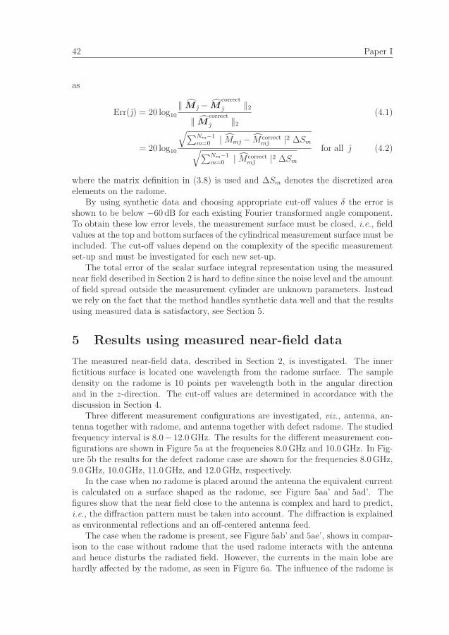
42 Paper I

as

Err(j) = 20 log10

‖ M j − Mcorrect

j ‖2

‖ Mcorrect

j ‖2

(4.1)

= 20 log10

√∑Nm−1m=0 | Mmj − M correct

mj |2 ΔSm√∑Nm−1m=0 | M correct

mj |2 ΔSm

for all j (4.2)

where the matrix definition in (3.8) is used and ΔSm denotes the discretized areaelements on the radome.

By using synthetic data and choosing appropriate cut-off values δ the error isshown to be below −60 dB for each existing Fourier transformed angle component.To obtain these low error levels, the measurement surface must be closed, i.e., fieldvalues at the top and bottom surfaces of the cylindrical measurement surface must beincluded. The cut-off values depend on the complexity of the specific measurementset-up and must be investigated for each new set-up.

The total error of the scalar surface integral representation using the measurednear field described in Section 2 is hard to define since the noise level and the amountof field spread outside the measurement cylinder are unknown parameters. Insteadwe rely on the fact that the method handles synthetic data well and that the resultsusing measured data is satisfactory, see Section 5.

5 Results using measured near-field data

The measured near-field data, described in Section 2, is investigated. The innerfictitious surface is located one wavelength from the radome surface. The sampledensity on the radome is 10 points per wavelength both in the angular directionand in the z-direction. The cut-off values are determined in accordance with thediscussion in Section 4.

Three different measurement configurations are investigated, viz., antenna, an-tenna together with radome, and antenna together with defect radome. The studiedfrequency interval is 8.0− 12.0 GHz. The results for the different measurement con-figurations are shown in Figure 5a at the frequencies 8.0 GHz and 10.0 GHz. In Fig-ure 5b the results for the defect radome case are shown for the frequencies 8.0 GHz,9.0 GHz, 10.0 GHz, 11.0 GHz, and 12.0 GHz, respectively.

In the case when no radome is placed around the antenna the equivalent currentis calculated on a surface shaped as the radome, see Figure 5aa’ and 5ad’. Thefigures show that the near field close to the antenna is complex and hard to predict,i.e., the diffraction pattern must be taken into account. The diffraction is explainedas environmental reflections and an off-centered antenna feed.

The case when the radome is present, see Figure 5ab’ and 5ae’, shows in compar-ison to the case without radome that the used radome interacts with the antennaand hence disturbs the radiated field. However, the currents in the main lobe arehardly affected by the radome, as seen in Figure 6a. The influence of the radome is

5 Results using measured near-field data 43

(a) (b)

b’

d’ e’

a’

f’

c’

10.0 GHz

8.0 GHz

10.0 GHz

12.0 GHz11.0 GHz

9.0 GHz8.0 GHz

Figure 5: The reconstructed currents in dB-scale [−30, 0], all normalized to thehighest current value, i.e., the maximum current magnitude in figure ac’. (a) Thedifferent measurement configurations are depicted at two different frequencies. Fromleft to right; antenna without radome, antenna together with radome, and antennatogether with defect radome, respectively. The arrows point out the location of thecopper plates on the defect radome. (b) The defect radome case, shown at differentfrequencies.

clearly visible in the reconstructed currents on the back of the radome where flashlobes occur, see Figure 6b.

The defect radome has two copper plates attached to its surface. These areplaced in the forward direction of the main lobe of the antenna and centered at theheights 41.5 cm and 65.5 cm above the bottom of the radome. The length of theside of the squared copper plates is 6 cm, which corresponds to 1.6 wavelengths at8.0 GHz and 2.4 wavelengths at 12.0 GHz, respectively. The locations of the copperplates are detected as shown in Figure 5ac’ and 5af’, where the lower plate appearsclearly. The other plate is harder to discern since it is placed in a region with smallcurrent magnitudes. However, a cross section graph through the main lobe detectseven this copper plate, see Figure 6a. Observe that the effects of the copper platescannot be localized directly in the near-field data, compare Figure 6a to Figure 3a.The near-field data only shows that the field is disturbed, not the location of thedisturbance. Nevertheless, by using the scalar surface integral representation theeffects of the plates are localized and focused. The defect radome also increases thebackscattering as seen in Figure 6b. Due to the copper plates the flash lobes aredifferent compared to the case with the non-defect radome.

44 Paper I

(a)

−0.7 −0.6 −0.5 −0.4 −0.3 −0.2 −0.1 0 0.1 0.2−40

−35

−30

−25

−20

−15

−10

−5

0

mag

nitu

de o

f rec

onst

ruct

ed fi

eld

/ dB

radome height / m

without radome with radome with defect radome

−0.7 −0.6 −0.5 −0.4 −0.3 −0.2 −0.1 0 0.1 0.2−40

−35

−30

−25

−20

−15

−10

−5

0m

agni

tude

of r

econ

stru

cted

fiel

d / d

B

radome height / m


(b)

lobesflash

mag

nitu

de o

f rec

onst

ruct

ed c

urre

nt /

dBdB

mag

nitu

de o

f rec

onst

ruct

ed c

urre

nt /

dBdB

radome height / mradome height / m

with radomewith defect radome

without radomewithout radome


Figure 6: Cross section of the reconstructed current on the radome surface forthe different measurement configurations, at 8.0 GHz. The current is shown asfunctions of the radome height for a fixed angle. All graphs are normalized to thehighest current value, i.e., the maximum current for the defect radome. (a) Thegraph representing the currents in the main lobe, i.e., the front of the radome. Theposition of the copper plates are marked as thick lines on the horizontal axis. (b) Thecurrents on the back of the radome.

As a final verification, the far-field amplitude on a sphere in the far-field region isstudied. The electric field, originating from the equivalent currents on the radome,is calculated on the sphere,

Esphj = −F−1

[GjM j

]for all j, j (5.1)

in accordance with (3.8) and (3.12), except that Gj now describes the transformationfrom the radome to the inner fictitious surface and the far field sphere, respectively.The denotions j and j are, as before, the integer index belonging to the discretizedangle component and the Fourier transformed discretized angle component, respec-tively.

The far-field amplitude F is derived as

F (θ, φ) = kr eikrEsph(r, θ, φ) as r → ∞ (5.2)

where (r, θ, φ) describes the spherical coordinate system [6]. The result is comparedwith far-field data, supplied by Chelton Applied Composites, as shown in Figure 7.The far field is depicted for the angles φ = 0 and φ = π, i.e., a cross-section throughthe far field of the main lobe and the corresponding far field originating from thecurrents on the back of the radome. There is a lack of agreement between themeasured far field and the calculated one in the angles corresponding to the topof the radome,i.e., θ ≈ 0. This is due to the fact that fields originating hereof arenot all included in the measured near-field data, since the measurement surface is a

6 Discussion and conclusions 45

−80 −60 −40 −20 0 20 40 60 80−40

−35

−30

−25

−20

−15

−10

−5

0

−80 −60 −40 −20 0 20 40 60 80−40

−35

−30

−25

−20

−15

−10

−5

0

−80 −60 −40 −20 0 20 40 60 80−40

−35

−30

−25

−20

−15

−10

−5

0

−80 −60 −40 −20 0 20 40 60 80−40

−35

−30

−25

−20

−15

−10

−5

0

calculated far field

far

fie

ld /

dB

theta / degree(a)

(d)c)

(b)

theta / degree theta / degree

theta / degreefa

r fiel

d / d

Bfa

r fiel

d / d

B

far fi

eld

/ dB

with radomewithout radome

defect radome

measured far fieldcalculated far field


measured far field

Figure 7: Comparison between the measured far-field data, supplied by CheltonApplied Composites, and the far field calculated from the equivalent currents on theradome surface. The far fields are normalized to the maximum value of the far fieldwhen no radome is present. (a) Antenna without radome. (b) Antenna togetherwith radome. (c) Antenna together with defect radome. (d) The calculated far-fieldpattern for the three measurement configurations.

cylinder, see Figure 2a. The fact that the radome disturbs and reflects the electricfield, as earlier seen in Figure 6b, can also be detected in the far field, see Figure 7d,where flash lobes appear when the radome is present.

6 Discussion and conclusions

The used scalar surface integral representation gives a linear map between the equiv-alent currents and the near-field data for general structures. It is here shown thatthis map can be inverted for axially symmetric geometries. The model can the-oretically be adapted to geometries lacking symmetry axes. Although it is not afeasible approach for radome applications, demanding large quantities of measureddata, with the present computer capacity.

46 Paper I

The transformation method is stable and useful in radome design and for eval-uation purposes. To investigate the electric field passing through the radome, thecurrent distribution on the antenna or on a surface enclosing the antenna mustbe known. Using the surface integral representation, the equivalent currents, on asurface enclosing the antenna, can be described.

Another range of application within the radome industry is to study how e.g.,lightning conductors and Pitot tubes, often placed on radomes, influence the equiv-alent currents. We show that such influences and the field effects of the radomeitself can be detected. In this paper, copper plates are attached on the radome, inthe direction of the antenna main lobe. The length of the side of the square copperplates are 1.6−2.4 wavelengths, corresponding to the frequency span 8.0−12.0 GHz.The effects of the plates cannot be localized directly by using the near-field data,but by using the equivalent currents the effects are focused and detected on theradome surface. Thus, by transforming the near-field data to the radome surface,field defects introduced by the radome and other disturbances are focused back totheir origins.

It is concluded that the transformation method based on the surface integralrepresentation works very well and that the field of applications is large. A nat-ural continuation is to elaborate the algorithm by including near field data withcross-polarization, i.e., to implement the full Maxwell equations with a Method ofMoments (MoM). Nevertheless, if the measured near-field data consists of one dom-inating component the use of the full Maxwell equations are not necessary, as shownin this paper.

Additional aspects to be investigated more thoroughly in the future are theresolution possibilities of manufacturing errors and other external field influences.Analysis of the phase information in the equivalent currents is also of interest. More-over, a study regarding the detection of different materials attached to the radomesurface is desirable.

Acknowledgments

The work reported in this paper is sponsored by Forsvarets Materielverk (FMV),Sweden, which is gratefully acknowledged.

The authors also like to express their gratitude to the people at SAAB BoforsDynamics, Sweden, and especially to Michael Andersson and Soren Poulsen at Chel-ton Applied Composites, Sweden, for supplying the near-field data and pictures ofthe experimental setup.

References

[1] H. Anton. Elementary Linear Algebra. John Wiley & Sons, New York, 7edition, 1994.

References 47

[2] C. A. Balanis. Antenna Theory. John Wiley & Sons, New York, second edition,1997.




[6] J. D. Jackson. Classical Electrodynamics. John Wiley & Sons, New York,second edition, 1975.


[8] R. Kress. Linear Integral Equations. Springer-Verlag, Berlin Heidelberg, secondedition, 1999.


[10] Y. Rahmat-Samii, L. I. Williams, and R. G. Yaccarino. The UCLA bi-polarplanar-near-field antenna-measurement and diagnostics range. IEEE Antennasand Propagation Magazine, 37(6), 16–35, December 1995.


[12] G. Strang. Introduction to applied mathematics. Wellesley-Cambridge Press,Box 157, Wellesley MA 02181, 1986.


[14] V. V. Varadan, Y. Ma, V. K. Varadan, and A. Lakhtakia. Scattering of wavesby spheres and cylinders. In V. V. Varadan, A. Lakhtakia, and V. K. Varadan,

48 Paper I

editors, Field Representations and Introduction to Scattering, volume 1 of Hand-book on Acoustic, Electromagnetic and Elastic Wave Scattering, chapter 4,pages 211–324. Elsevier Science Publishers, Amsterdam, 1991.


[16] A. D. Yaghjian. An overview of near-field antenna measurements. IEEE Trans.Antennas Propagat., 34(1), 30–45, January 1986.

Paper II

Reconstruction ofequivalent currents usingthe scalar surface integralrepresentation

Kristin Persson and Mats Gustafsson

Based on: K. Persson and M. Gustafsson. Reconstruction of equivalent currentsusing the scalar surface integral representation, Technical Report LUTEDX/(TEAT-7131), pp. 1–25, 2005, Department of Electrical and Information Technology, LundInstitute of Technology, Sweden. http://www.eit.lth.se

1 Introduction 51

Abstract

Knowledge of the current distribution on a radome can be used to improveradome design, detect manufacturing errors, and to verify numerical simula-tions. In this paper, the transformation from near-field data to its equivalentcurrent distribution on a surface of arbitrary material, i.e., the radome, isanalyzed. The transformation is based on the scalar surface integral represen-tation that relates the equivalent currents to the near-field data. The presenceof axial symmetry enables usage of the fast Fourier transform (FFT) to reducethe computational complexity. Furthermore, the problem is regularized usingthe singular value decomposition (SVD). Both synthetic and measured dataare used to verify the method. The quantity of data is large since the heightof the radome corresponds to 29 − 43 wavelengths in the frequency interval8.0 − 12.0 GHz. It is shown that the method gives an accurate descriptionof the field radiated from an antenna, on a surface enclosing it. Moreover,disturbances introduced by copper plates attached to the radome surface, notlocalized in the measured near field, are focused and detectable in the equiva-lent currents. The method also enables us to determine the phase shift of thefield due to the passage of the radome, cf., the insertion phase delay.

1 Introduction

This paper provides a wrap-up and a final report of the reconstruction of equivalentcurrents in the scalar approximation. The theoretical derivation is a summary ofthe work [11]. The new aspect in this report is mainly the analysis of the measurednear-field data, especially the investigation of the phase information. Different waysof visualizing the results are also discussed and presented.

1.1 Ranges of application

There are several applications of a near field to equivalent currents transformation.For example, in the radome industry it is important to have accurate models of thefield radiated from the antenna placed inside the radome. It is hard to measurethis field directly since the radome often is located very close to the antenna andat these distances, there is a substantial interaction between the antenna and themeasuring probe [6, 13, 19]. It is also important to have a powerful tool to determinethe insertion phase delay (IPD), also known as the electrical thickness of the radome.The IPD is often one of the specified qualities given to characterize a radome. Oneway to measure the IPD is to place two horn antennas in such a way that theincident angle on the radome coincide with the Brewster angle, which is the anglewhere the transmitted field has its highest value [12]. To get the IPD, the phaseof the transmitted field is subtracted from the phase of the measured field with noradome between the horn antennas. This process is very time consuming since ithas to be repeated several times to cover the whole radome surface. Using the scalarsurface integral equation, the phase shift due to the propagation through the radomeis determined.

52 Paper II

Another field of application is in the manufacturing of radiating bodies, i.e.,antenna arrays etc., when the radiation pattern from the body does not exhibit theexpected form. By determination of the equivalent currents on the radiating body,the malfunctioning areas or components can be found.

1.2 History

A common method, transforming near field to equivalent currents and vice versa,is to use modal-expansions of the electric field [6]. This is a very efficient methodfor radiating bodies with certain geometrical symmetries, i.e., planar, cylindrical,and spherical. Having a planar aperture, the plane wave spectrum of the fieldis utilized in the back transformation [3, 5]. The fact that the expression of thefar field originating from a planar surface is equal to the Fourier transform of theradiating field on the aperture has been investigated in [10, 13]. The paper [10] alsoillustrates that defects, i.e., patches of Eccosorb, can be detected on the aperture. Ifthe radiating body is of cylindrical or spherical geometry, the radial solutions containcylindrical and spherical Bessel functions, while the angular solutions are describedby trigonometric functions and the associated Legendre functions [6, 17]. For generalgeometrical symmetries, where modal-expansions do not exist, the modal-expansionis less applicable.

Moreover, different combinations of the electric- and magnetic-field integral equa-tions (EFIE and MFIE) derived from the Maxwell equations, have been used to backpropagate fields towards their sources, i.e., a linear inverse source problem is solved.By this method it is possible to handle a wider class of geometries [13]. In [18] thedual-surface, magnetic and electric-field integral equations are investigated. Thefields are transformed back to a cubic perfect electric conductor by solving the dual-surface magnetic-field integral equation using the conjugate gradient method. Otherwork using the integral equations is reported in [14], where the near field is measuredon a arbitrary surface and later inverted to a planar, perfectly conducting surfaceby using a singular value decomposition (SVD) for regularization.

1.3 The scalar surface integral representation

In this paper, the approach is to investigate a scalar surface integral representationthat does not require the aperture to be a perfect electric or magnetic conductor.The representation provides a relation relating the unknown electric and magneticequivalent currents on a surface to the measured electric field. An additional relationis given by the fact that the equivalent currents are constructed such that the integralis zero inside the volume, on which surface the currents exist, i.e., the extinctiontheorem [16].

The integral relations are discretized into matrix linear equations. The matrixequations include an azimuthal convolution which is solved with a fast Fourier trans-form (FFT) in the angular coordinate. The fast Fourier transform brings down thecomplexity of the problem, i.e., the original surface-to-surface linear map is decom-posed into a set of line-to-line linear maps. A singular value decomposition (SVD)

1 Introduction 53

−0.8 −0.6 −0.4 −0.2 0 0.2 0.4 0.6 0.8−40

−35

−30

−25

−20

−15

−10

−5

0

−3 −2 −1 0 1 2 3−40

−35

−30

−25

−20

−15

−10

−5

0

−3 −2 −1 0 1 2 3−40

−35

−30

−25

−20

−15

−10

−5

0

−0.8 −0.6 −0.4 −0.2 0 0.2 0.4 0.6 0.8−40

−35

−30

−25

−20

−15

−10

−5

0


mag

nitu

de o

f mea

sure

dco

−pol

ariz

ed fi

eld

/ dB

(d)

mag

nitu

de o

f mea

sure

d

mag

nitu

de o

f mea

sure

dcr

oss−

pola

rized

fiel

d / d

Bm

agni

tude

of m

easu

red

cros

s−po

lariz

ed fi

eld

/ dB

(a) (b)

(c)

co−p

olar

ized

fiel

d / d

B


cylinder height / m cylinder height / m


with defect radome

without radomewith radome

without radome

without radome

without radome

with defect radomewith radomewith radome

with defect radome

Figure 1: The measured co- and cross-polarized electric field on the measurementcylinder at 8.0 GHz. In (a) and (b) the angle is fixed at ϕ = 0, and the fields arenormalized by the maximum value when no radome is present in (a). In (c) and (d)the height is fixed at z = 0, and the fields are normalized to the maximum valuewhen no radome is present in (c).

is used to invert each of these linear maps. As most inverse problems it is ill-posed,i.e., small errors in the near-field data can produce large errors in the equivalentcurrents. Thus, the problem needs to be regularized by suppression of small singularvalues when inverted.

1.4 Results

In this paper, the measured electric field is presumed to be scalar, i.e., the scalarsurface integral representation is utilized. The assumption is acceptable since theused near-field data, supplied by SAAB Bofors Dynamics and Applied CompositesAB, Sweden, clearly have one dominating component in the main lobe, see Figure 1.The measured data is given for three different antenna and radome configurations,viz., antenna, antenna together with radome, and antenna together with defectradome. The measurement set-up is shown in Figure 2. The height of the radome

54 Paper II

Figure 2: Photo of the cylindrical near-field range at SAAB Bofors Dynamics,Sweden. The antenna under test is rotated and the probe is moved in the verticaldirection. A close up of the reflector antenna is shown in the upper right corner.

corresponds to 29 − 43 wavelengths in the frequency interval 8.0 − 12.0 GHz.As a start, synthetic data is used to verify the method. Verification is also

performed by a comparison between the measured far field and the far field calculatedfrom the equivalent currents on the radome. The calculated far field agrees wellwith the measured far field. Moreover, when the radome is introduced, the field isscattered and flash lobes arise. The equivalent currents on the radome, due to theseeffects are identified and the flash lobes are accurately detected.

Manufacturing errors, not localized in the measured near-field data, can be fo-cused and detected in the equivalent currents on the radome surface. In this paper,it is shown that the field scattered by copper plates attached on the radome, isfocused back towards the original position of the copper plates. The length of theside of the square copper plates is 6 cm, i.e., 1.6− 2.4 wavelengths corresponding tothe frequency span 8.0 − 12.0 GHz.

1.5 Outline

In Section 2, the experimental set-up is described and the measured near-field datais presented. The scalar surface integral representation is introduced and adapted tothe specific problem in Section 3. Section 4 contains the implementation process ofthe scalar surface integral representation. Results, using synthetic near-field data,and the error of the method are presented. The results, when using the experimentalnear-field data, are shown and examined in Section 5. To give the reader a under-standing of the information that can be extracted from the resulting data, Section 6gives examples of ways to visualize the results. The paper ends with the achieved


a) b)

zizm

zp

ϕn

ϕj

ϕj

z/mm

800

342

0

-728-800

ρ/mm0 213 459

33

320

0 ≤ i ≤ Ni − 10 ≤ j ≤ Nj − 10 ≤ m ≤ Nm − 10 ≤ n ≤ Nn − 10 ≤ p ≤ Np − 1

Figure 3: (a) The dimensions of the reflector antenna, the radome, and thecylinder where the electric near field is measured. (b) A close-up showing the innerfictitious surface and the discretized geometric variables.

conclusions in Section 7.


The near-field data, used in this paper, was supplied by SAAB Bofors Dynamics andApplied Composites AB, Sweden. The set-up with relevant dimensions indicated isshown in Figures 2 and 3a. Three different measurements were performed; datameasured without the radome, data measured with the radome, and data measuredwith the defect radome. The defect radome has two copper plates attached to itssurface.

A reflector antenna, fed by a symmetrically located wave-guide, generates thenear-field, see Figure 2. The diameter of the antenna is 0.32 m and its focal distanceis 0.1 m. The main lobe of the antenna is vertically polarized relative to the hori-zontal plane. The standing wave ratio (SWR) is approximately 1.4 in the frequencyrange 8.2 − 9.5 GHz. The antenna is poorly adapted for other frequencies. A 10 dBreflection attenuator is connected to the antenna.

56 Paper II

The height of the radome surface is modeled by

ρ(z) =

{0.213 m −0.728 m ≤ z ≤ −0.663 m

−(bz′ + d) +√

(bz′ + d)2 − a(z′)2 − 2cz′ − e −0.663 m < z ≤ 0.342 m

(2.1)where z′ = z + 0.728 m and the constants are a = 0.122, b = 0.048, c = −0.018 m,d = 0.148 m, and e = −0.108 m2, respectively. The material of the radome has arelative permittivity of 4.32 and its loss tangent is 0.0144. The thickness of thewall of the radome varies between 7.6− 8.2 mm. The near-field measurement probeconsists of a wave-guide for which no compensation is made in the final data. Thecylindrical surface, where the electric field is measured, is located in the near-fieldzone [2].

The amplitude and phase of the electric field are measured in the frequency in-terval 8.0−12.0 GHz on a cylindrical surface by moving the probe in the z-directionand rotating the antenna under test, see Figure 2. With this measurement set-up,the fields on the top and the bottom of the cylindrical surface could not be col-lected. It would have been preferable to measure the fields on an infinite cylinder.However, the size of the cylinder is chosen such that the turntable below the radomedoes not have a major influence of the measurements and such that the fields abovez = 800 mm are negligible, cf., Figures 1 and 3a. In the azimuth angle, 120 pointsare measured between −180◦ and 180◦ in steps of 3◦. The z-dimension is dividedinto 129 points, separated by 12.5 mm. This means that at 8.0 GHz the electricfield is measured 3 times per wavelength, in the z-direction, and 1.5 times per wave-length, in the azimuth direction, respectively. Together, a total of 120×129 = 15480measurement points are used for each radome configuration and frequency. The co-and cross-polarized measured electric fields are shown in Figure 1. The differencesbetween the three different antenna and radome cases arise from constructive anddestructive interference between the radiated field and the scattered field. In Fig-ure 1 it is also observed that the electric field consists of a dominating co-componentin the main lobe, i.e., a dominating z-component since the antenna is vertically po-larized.

3 The surface integral representation

The surface integral representation expresses the electromagnetic field in a homoge-neous, isotropic region in terms of its values on the bounding surface. The represen-tation states that if the electromagnetic field on a surface of a volume is known, theelectromagnetic field in the volume can be determined [8, 16]. The representation isderived starting from the time harmonic Maxwell equations with the time conventioneiωt. The Maxwell equations transform into the vector Helmholtz equation

∇2E(r) + k2E(r) = 0 (3.1)

since the material (air) is source free, homogeneous, and isotropic.


Assume that the electric field only consists of a component in the z-direction.This is a good approximation dealing with the specific measurements described inSection 2 since our prime interest is to reconstruct the electric field in the main lobe,where the z-component is clearly the dominating one, cf., Figure 1.

Working with a scalar field, the surface integral representation only depends onthe scalar electric field, Ez, and its normal derivative, ∂Ez/∂n, i.e., not all compo-nents of the electric and magnetic fields need to be included. Observe that in thevector integral representation all tangential components of the electric and magneticfields must be taken into account [8]. The scalar surface integral representation isderived using the free space Green function g(r, r′) = e−ik|r−r′|/4π|r−r′| giving [16]

ˆˆ

S

[∂g(r, r′)∂n

Ez(r) − g(r, r′)∂Ez(r)

∂n

]dS =

{−Ez(r

′) r′ ∈ V

0 r′ /∈ V(3.2)

where V is the volume exterior to the closed surface S which consists of the radomesurface with an added top and bottom surface. Observe that the electric field doesnot have to be zero outside the volume, i.e., inside the radome. The surface integralrepresentation (3.2) only states that the left-hand side of the equation, evaluated ata point r′ outside the volume V , is zero, i.e., the extinction theorem [16].

The equivalent surface currents are introduced as

M(r) ≡ Ez(r) and M ′(r) ≡ ∂Ez(r)

∂n(3.3)

which inserted in (3.2) give

ˆˆ

radome

[∂g(r, r′)∂n

M(r) − g(r, r′)M ′(r)

]dS =

{−Ecyl

z (r′) r′ ∈ cylinder

0 r′ ∈ inside radome(3.4)

where Ecylz is the z-component of the electric field on the measurement cylinder.

The fictitious surface, inside the radome, is shaped as the radome and located closeto the radome wall.

3.1 Angular Fourier transformation

Due to the measurement set-up, the transformation, the Green’s function, is axiallysymmetric, see Section 2. The symmetry only applies to the transformation, notto the electric field. Thus, the left-hand side in (3.4) represents a convolution andby using a Fourier transformation of the azimuth coordinate, the computationalcomplexity can be brought down one dimension. This reduction of one dimension,can be understood by writing the left-hand side in (3.4) as a matrix, X. This matrixis a circulant matrix, i.e., every row is shifted one step to the right compared tothe previous row. The eigenvectors of all circulant matrices are the column vectorsof the Fourier matrix, F . Multiplying a circulant matrix with the Fourier matrix,i.e., performing the Fourier transformation, gives FX = FΛ where Λ is a diagonalmatrix, which can be seen as a reduction of one dimension [15].

58 Paper II

The continuous variables in (3.4) are discretized to give linear matrix equations.The discretized cylindrical coordinate system is described by the integer indicesdepicted in Figure 3b. Discretization and Fourier transformation, in the azimuthcoordinate, of (3.4) give

Nm−1∑m=0

[G ′

imjMmj − GimjM′mj

]= −Ecyl


andNm−1∑m=0

[G′

pmjMmj − GpmjM′mj

]= 0 for all p, j (3.6)

where G and G are the surface integrals, taken over the radome, of the Green’sfunction multiplied with the basis functions used in the discretization process. G hasthe discretized space variable r′ belonging to the measurement cylinder and G hasthe discretized space variable r′ belonging to the fictitious surface inside the radome,respectively. The prime denotes the normal derivative of the Green’s function, j isthe integer index belonging to the Fourier transformed azimuth component, and the“hat” denotes the Fourier transformed variables. The summation limits Nm and Np

are given in Figure 3b.To solve the scalar surface integral representation, a limit process of (3.6) should

be performed, letting the fictitious surface inside the radome approach the radomesurface [2, 9]. To avoid singularities, we let the fictitious surface be located at afinite distance from the radome surface. This provides us with a simple and feasiblemethod to allocate the surface currents, i.e., the extinction theorem is used as anapproximate solution to the integral representation in (3.6).

Reduction of M ′ in (3.5) and (3.6) gives

Nm−1∑m=0

{G ′

imj −Np−1∑p=0

Nm−1∑q=0

Giqj (G−1)qpj G′pmj

}Mmj = −Ecyl


Equation (3.7) can also be written as j matrix equations

Gradome

j M j = −Ecyl

j for all j (3.8)

where the matrices are defined as M j ≡ [Mm1]j, Ecyl

j ≡ [Ecyli1 ]j, and

Gradome

j ≡ [G ′im]j − [Gim]j[Gmp]

−1j [G′

pm]j for all j (3.9)

The used notation of matrices is that of [1].

3.2 Inversion with singular value decomposition

Since the matrices Gradome

j and [Gmp]j in (3.8) and (3.9) are not quadratic, a regularinversion cannot be performed. A fast and easy way to solve this is to use the

4 Implementation 59

singular value decomposition (SVD) [15]. This method is used on both matrices,

but the SVD-equations are only given here for Gradome

j . The matrix system (3.8)can then be rewritten as

U jS jV†jM j = −E

cyl

j for all j (3.10)

where V†j denotes the Hermitian conjugate of V j. Both U j and V j are orthogonal

matrices. S j is a diagonal matrix consisting of the singular values to Gradome

j in de-

creasing order. The singular values of both Gradome

j and [Gmp]j exhibit the tendencyshown by the curves in Figure 4a.

A cut-off value, δ, normalized to the operator L2-norm of Gradome

1 is chosen. The

operator L2-norm of Gradome

1 is equal to the largest singular value (σ1) of the largestFourier transformed azimuth component [9]. All singular values smaller than δ are

ignored during the inversion of S j and are afterwards set to zero. If this is not donethe small singular values create an uncontrolled growth of non-radiation currentswhen inverted. The mathematical formulation then fails since very small electricfield contributions become dominating. Performing the inversion of (3.10) gives

M j = − V jS−1

j U†jE

cyl

j for all j (3.11)

Before the system of equations is solved, it is necessary to convert it back fromFourier space by an inverse Fourier transformation

M j = F−1

[−V jS

−1

j U†jE

cyl

j

]for all j, j (3.12)

where j, as above, denotes the integer index belonging to the discretized azimuthcomponent, see Figure 3b.

4 Implementation

Some adjustments of the formulas are made in the implementation process. Tofacilitate the calculations, the radome surface is reshaped into a closed surface byadding a smooth top and bottom surface. These extra surfaces are useful since themeasurements are performed under non-ideal conditions. The turntable, on whichthe antenna and radome are located, see Figure 2, reflects some of the radiation,which is taken care of by the added bottom surface. The top surface takes care of theelectric field that is reflected on the inside of the radome and then radiated throughthe top hole. If these factors are not considered, unwanted edge effects occur sincethe electric field originating from the turntable and the top of the radome is forcedto arise from the radome itself.

The measured electric near field is only measured 1.5 times per wavelength, inthe azimuth direction, at the frequency 8.0 GHz, see Section 2. To be sure that the

60 Paper II

10 20 30 40 50 60 70−80

−60

−40

−20

0

mag

nitu

de o

f sin

gula

r va

lue

/ dB

singular value

σ1

(a) (b) (c)

Figure 4: (a) The typical behavior of singular values of Gradome

j and [Gmp]j. Everycurve represents the singular values of a Fourier transformed azimuth component,i.e., different j. The horizontal lines describe the cut-off values, δ = σ1[0.15 0.1 0.050.01 0.005]. (b) The synthetic equivalent currents, originating from three dipoles, ina dB-scale [−15, 0], normalized to the highest current value, i.e., the maximum cur-rent magnitude in subfigure c. (c) The reconstructed currents in dB-scale [−15, 0],normalized to its highest current value.

equivalent currents on the radome are recreated in an accurate way, it is necessary tohave a high sample density on the radome. This is achieved by increasing the numberof discrete points, in the azimuth direction, on the radome surface by including extraangles between the already existing ones. Thus, the axial symmetry of the Green’stransformation is preserved.

The sample density on the measurement cylinder contributes very little to thetotal error. The scalar surface integral representation creates currents on the radomesuch that the electric field is correct at the measurement points. However, if theNyquist theorem is fulfilled, then the electric field is correct at all points on themeasurement surface, i.e., not only at the measurement points [15]. As mentioned

above, the amount of data is large and the matrix Gradome

, cf., (3.9), has approxi-mately 108 elements at the frequency 8.0 GHz when the sample density is 10 pointsper wavelength both in the azimuth direction and in the z-direction on the radome.

To verify and find the error of the method, synthetic data is used. A syntheticelectric field, originating from three dipoles inside the radome is shown in Figure 4b.The corresponding reconstructed currents on a surface shaped as the radome areshown in Figure 4c where the sample density is 10 points per wavelength both inthe z-direction and in the azimuth direction. The inner fictitious surface is locatedone wavelength from the radome surface.

The error as a function of the Fourier transformed azimuth angle component is

4 Implementation 61

(a) (b)

b’

d’ e’

a’

f’

c’

10.0 GHz

8.0 GHz

10.0 GHz

12.0 GHz11.0 GHz

9.0 GHz8.0 GHz

Figure 5: The reconstructed currents in dB-scale [−30, 0], all normalized to thehighest current value, i.e., the maximum current magnitude in figure ac’. (a) Thedifferent measurement configurations are depicted at two different frequencies. Fromleft to right; antenna without radome, antenna together with radome, and antennatogether with defect radome, respectively. The arrows point out the location of thecopper plates on the defect radome. (b) The defect radome case, shown at differentfrequencies.

defined as

Err(j) = 20 log10

‖ M j − Mcorrect

j ‖2

‖ Mcorrect

j ‖2

= 20 log10

√∑Nm−1m=0 | Mmj − M correct

mj |2 ΔSm√∑Nm−1m=0 | M correct

mj |2 ΔSm

for all j

(4.1)

where ΔSm denotes the discretized area elements on the radome.By using synthetic data and choosing appropriate cut-off values, δ, the error is

shown to be below −60 dB for each existing Fourier transformed azimuth angle com-ponent. To obtain these low error levels, the measurement surface must be closed,i.e., field values at the top and bottom surfaces of the cylindrical measurement sur-face must be included. The cut-off values depend on the complexity of the specificmeasurement set-up and must be investigated for each new set-up.

The total error of the scalar surface integral representation using the measurednear field described in Section 2 is hard to define since the noise level and the amount

62 Paper II

(a)

−0.7 −0.6 −0.5 −0.4 −0.3 −0.2 −0.1 0 0.1 0.2−40

−35

−30

−25

−20

−15

−10

−5

0

mag

nitu

de o

f rec

onst

ruct

ed fi

eld

/ dB

radome height / m


−0.7 −0.6 −0.5 −0.4 −0.3 −0.2 −0.1 0 0.1 0.2−40

−35

−30

−25

−20

−15

−10

−5

0m

agni

tude

of r

econ

stru

cted

fiel

d / d

B

radome height / m


(b)

lobesflash

mag

nitu

de o

f rec

onst

ruct

ed c

urre

nt /

dBdB

mag

nitu

de o

f rec

onst

ruct

ed c

urre

nt /

dBdB

radome height / mradome height / m

with radomewith defect radome

without radomewithout radome


Figure 6: Cross section of the reconstructed currents, on the radome surface, forthe different measurement configurations at 8.0 GHz. The currents are shown asfunctions of the radome height for a fixed angle. All graphs are normalized to thehighest current value, i.e., the maximum current for the defect radome case. (a) Thegraph representing the currents in the main lobe, i.e., the front of the radome. Thepositions of the copper plates are marked by thick lines on the horizontal axis.(b) The currents on the back of the radome.

of field spread outside the measurement cylinder are unknown parameters. Instead,we rely on the fact that the method handles synthetic data well and that the resultsusing measured data is satisfactory, see Section 5.

5 Results using measured near-field data

The measured near-field data, described in Section 2, is investigated. The innerfictitious surface is located one wavelength from the radome surface. The sampledensity on the radome is 10 points per wavelength both in the azimuth directionand in the z-direction. The cut-off values are determined in accordance with thediscussion in Section 4.

Three different measurement configurations are investigated, viz., antenna, an-tenna together with radome, and antenna together with defect radome. The studiedfrequency interval is 8.0− 12.0 GHz. The results for the different measurement con-figurations are shown in Figure 5a at the frequencies 8.0 GHz and 10.0 GHz. In Fig-ure 5b the results for the defect radome case are shown for the frequencies 8.0 GHz,9.0 GHz, 10.0 GHz, 11.0 GHz, and 12.0 GHz, respectively.

In the case when no radome is located around the antenna, the equivalent cur-rents are calculated on a surface shaped as the radome, see Figure 5aa’ and 5ad’.The figures show that the near field close to the antenna is complex and hard topredict, i.e., the diffraction pattern must be taken into account. The diffraction isexplained as environmental reflections and an off-centered antenna feed.

The case when the radome is present, see Figure 5ab’ and 5ae’, shows in com-


a’ b’

(b)

8.0 GHz 9.0 GHz 10.0 GHz

11.0 GHz 12.0 GHz

c’

d’ e’ f’

8.0 GHz

10.0 GHz

(a)

0

π

−π

Figure 7: The reconstructed phase of the currents on the front of the radome.(a) The different measurement configurations are depicted at two different frequen-cies. From left to right; antenna without radome, antenna together with radome,and antenna together with defect radome, respectively. (b) The defect radome case,shown at different frequencies.

parison to the case without radome that the radome interacts with the antenna andhence disturbs the radiated field. However, the currents in the main lobe are hardlyaffected by the radome, as seen in Figure 6a. The influence of the radome is clearlyvisible in the reconstructed currents on the back of the radome where flash lobesoccur, see Figure 6b.

The defect radome has two copper plates attached to its surface. These arelocated in the forward direction of the main lobe of the antenna and centered atthe heights 41.5 cm and 65.5 cm above the bottom of the radome. The length of theside of the squared copper plates is 6 cm, which corresponds to 1.6 wavelengths at8.0 GHz and 2.4 wavelengths at 12.0 GHz, respectively. The locations of the copperplates are detected as shown in Figure 5ac’ and 5af’, where the lower plate appearsclearly. The other plate is harder to discern since it is located in a region with lowamplitudes. However, a cross section graph through the main lobe detects even thiscopper plate, see Figure 6a. Observe that the effects of the copper plates cannot belocalized directly in the near-field data, compare Figure 6a to Figure 1a. The near-field data only shows that the field is disturbed, not the location of the disturbance.Nevertheless, by using the scalar surface integral representation, the effects of theplates are localized and focused. The defect radome also increases the backscatteringas seen in Figure 6b. Due to the copper plates, the flash lobes are different comparedto the case with the non-defect radome.

Until now only the amplitude of the reconstructed currents has been investigated.The phase of the currents is depicted in Figure 7. The vertical lines above themain lobe in Figure 7a’ and 7d’ are due to phase jumps and are caused by the low

64 Paper II

π

0

−π

Front

Back

8.0 GHz 9.0 GHz 10.0 GHz 11.0 GHz 12.0 GHz

Figure 8: The phase difference (antenna - antenna with radome) for severalfrequencies.

amplitude of the currents in these areas. The phase difference (antenna - antennawith radome) reveals how the the phase is changed due to the influence of theradome, see Figure 8. The phase shift, denoted Δϕ, is only known modulus 2π. Thephase shift in the main lobe is almost constant, especially for the low frequencies,which is more clearly seen by looking at the cross section of the front side of theradome, see Figure 9. What is noticeable in this image is the region between z =−0.4 m and z = 0 m, i.e., the main lobe where the phase shift is nearly constant.In areas where the amplitude of the field is small, cf., Figure 6a, the phase of thefield is not well defined, i.e., it is dominated by noise. This almost constant phaseshift, for the low frequencies, confirms that the radome is quite well adapted to thefrequencies 8.0− 9.0 GHz, which is also the frequency interval where the antenna iswell matched, see Section 2.

Sometimes, when dealing with phase information, the figures can be clarified byusing phase unwrapping [4]. It means that the jump in the scale between 0 and 2πis removed. In our case phase unwrapping gives us no new information since thearea of interest is the main lobe and the phase shift there is almost constant.

To validate the calculation of the phase shift, the propagation distance of thefield through the radome, i.e., the actual propagation path of the field in the radomematerial, is estimated and compared to the actual thickness of the radome given inSection 2. The propagation distance of the field through the radome is longer thanthe wall thickness since the field has an incident angle larger than zero. The phasedifference between two fields propagating the distance d in air and in the radomematerial, respectively, can be written as [12]

Δϕ = Re[2πf

√ε0εrμ0(1 − i tan δ)

]d− 2πf

√ε0μ0 d (5.1)

where f is the frequency, d the propagation distance of the field, ε0 the permittivity of


−0.6 −0.4 −0.2 0 0.2−3

−2

−1

0

1

2

3

phas

e di

ffere

nce

/ rad

radome height / m

8.0 GHz 9.0 GHz 10.0 GHz11.0 GHz12.0 GHz

Figure 9: Cross section of the phase difference (antenna - antenna with radome)on the front of the radome. Observe that in areas where the amplitude of thecurrents are small, cf., Figure 6a, the phase of the field is not well defined, i.e., it isdominated by noise.

π

0

−π

Front

Back

9.0 GHz 10.0 GHz 11.0 GHz 12.0 GHz8.0 GHz

Figure 10: The phase difference (antenna with radome - antenna with defectradome) for several frequencies. The arrows point out the location of the copperplates.

66 Paper II

vacuum, and μ0 the permeability of vacuum, respectively. The parameters belongingto the radome, described in Section 2, are the relative permittivity, εr, and the losstangent, tan δ. Since only an estimation of the propagation distance is performed,we assume that this distance is the same in both air and the radome material. Weassume perpendicular incidence and neglect all reflections. According to Section 2,the thickness of the radome is between 7.6 − 8.2 mm. The almost constant phaseshifts in the main lobe are approximated from Figure 9 for all frequencies. Solvingfor d in (5.1) results in a propagation distance of 9.3 − 9.7 mm for all frequencies,which is considered constant due to the crude approximations of the phase shifts.The phase shift, Δϕ, is comparable to the insertion phase delay (IPD) often used inthe radome industry.

The phase images in Figure 7b are not appropriate for finding the location of thecopper plates. Instead, the phase difference (antenna with radome - antenna withdefect radome) is useful, see Figure 10. These images reveal the change of the phasedue to the attached copper plates on the defect radome.

As a final verification of the method, the amplitude on a sphere in the far-fieldregion is studied. The electric field, originating from the equivalent currents on theradome, is calculated on the sphere, i.e.,

Esphj = −F−1

[GjM j

]for all j, j (5.2)

in accordance with (3.8) and (3.12), except that Gj now describes the transformationfrom the radome to the inner fictitious surface and to the far-field sphere. Thedenotions j and j are, as above, the integer index belonging to the discretizedazimuth component and the Fourier transformed discretized azimuth component,respectively.

The far-field amplitude F is derived as

F (θ, φ) = kr eikrEsph(r, θ, φ) as r → ∞ (5.3)

where (r, θ, φ) denotes the spherical coordinate system [7]. The result is comparedwith far-field data, supplied by Applied Composites AB, as shown in Figure 11. Thefar field is depicted for the angles φ = 0 and φ = π, i.e., a cross-section throughthe far field of the main lobe and the corresponding far field originating from thecurrents on the back of the radome. There is a lack of agreement between themeasured far field and the calculated one at the angles corresponding to the top ofthe radome, i.e., θ ≈ 0. This is due to the fact that fields originating hereof arenot all included in the measured near-field data, since the measurement surface is acylinder, see Figure 3a. The fact that the radome disturbs and reflects the electricfield, as earlier seen in Figure 6b, can also be detected in the far field, see Figure 11d,where flash lobes appear when the radome is present.

6 Alternative ways to visualize the electromagnetic currents 67

−80 −60 −40 −20 0 20 40 60 80−40

−35

−30

−25

−20

−15

−10

−5

0

−80 −60 −40 −20 0 20 40 60 80−40

−35

−30

−25

−20

−15

−10

−5

0

−80 −60 −40 −20 0 20 40 60 80−40

−35

−30

−25

−20

−15

−10

−5

0

−80 −60 −40 −20 0 20 40 60 80−40

−35

−30

−25

−20

−15

−10

−5

0

calculated far field

far

fie

ld /

dB

theta / degree(a)

(d)c)

(b)

theta / degree theta / degree

theta / degree

far fi

eld

/ dB

far fi

eld

/ dB

far fi

eld

/ dB

with radomewithout radome

defect radome



measured far field

Figure 11: Comparison between the measured far-field data, supplied by AppliedComposites AB, and the far field calculated from the equivalent currents on theradome surface. The far fields are normalized to the maximum value of the far fieldwhen no radome is present. (a) Antenna without radome. (b) Antenna togetherwith radome. (c) Antenna together with defect radome. (d) The calculated far-fieldpattern for the three measurement configurations.

6 Alternative ways to visualize the electromag-

netic currents

6.1 Amplitude of the reconstructed currents

In the previous section, the amplitude and the phase of the reconstructed currentshave been visualized by showing the amplitude in dB-scale over the front side of theradome in Figure 5, and over a cross section of the front and the back in Figure 6.These ways of presenting the results are in this section supplemented in an attemptto see what possibilities other visualization approaches offer. First, the back side ofthe radome is shown in a dB-scale in Figure 12. The absolute value of the currents isalso displayed in a linear scale on the front and the back of the radome in Figures 13

68 Paper II

a’ 10.0 GHzb’

12.0 GHz

c’

d’ e’ f’

8.0 GHz

10.0 GHz

(a) (b)

8.0 GHz 9.0 GHz

11.0 GHz

Figure 12: The reconstructed currents on the back of the radome in a dB-scale[−30, 0], all normalized to the highest current value, i.e., the maximum current mag-nitude in Figure 5ac’. (a) The different measurement configurations are depicted attwo different frequencies. From left to right; antenna without radome, antenna to-gether with radome, and antenna together with defect radome, respectively. (b) Thedefect radome case, shown at different frequencies.

a’ b’ 9.0 GHz 10.0 GHz

11.0 GHz 12.0 GHz

c’

d’ e’ f’

8.0 GHz

10.0 GHz

(a) (b)

8.0 GHz

Figure 13: The reconstructed currents on the front of the radome in a linear scale,all normalized to the highest current value, i.e., the maximum current magnitudein figure ac’. (a) The different measurement configurations are depicted at twodifferent frequencies. From left to right; antenna without radome, antenna togetherwith radome, and antenna together with defect radome, respectively. The arrowspoint out the location of the copper plates on the defect radome. (b) The defectradome case, shown at different frequencies.

6 Alternative ways to visualize the electromagnetic currents 69

a’ 10.0 GHzb’

12.0 GHz

c’

d’ e’ f’

8.0 GHz

10.0 GHz

(a) (b)

8.0 GHz 9.0 GHz

11.0 GHz

Figure 14: The reconstructed currents on the back of the radome in a linear scale,all normalized to the highest current value, i.e., the maximum current magnitudein Figure 13ac’. (a) The different measurement configurations are depicted at twodifferent frequencies. From left to right; antenna without radome, antenna togetherwith radome, and antenna together with defect radome, respectively. (b) The defectradome case, shown at different frequencies.

and 14, respectively. The flash lobes clearly appear in both dB- and linear scale, seeFigures 12 and 14. Notice that the top copper plate is not resolved very well in thelinear scale compared to the dB-scale in Figure 5.

6.2 Differences between the measurement configurations

To further demonstrate the distinctions between the three radome configurationstheir differences are calculated. The difference (|antenna| - |antenna with radome|)is shown in Figure 15 in a dB-scale, and in Figure 16 in a linear scale. The imagesshow the influence of the radome and the appearance of flash lobes at the back ofthe radome. The dB-scale, Figure 15, has the advantage that also small currentvalues are made visible. The advantage with the linear scale is that the sign of thedifference is visible. In Figure 16, on the front of the radome, the field originatingfrom the antenna is the strongest, i.e., the difference is positive, while on the backof the radome, the field passing trough the radome as flash lobes is the strongest,i.e., the difference is negative. This conclusion can not be drawn by looking at thedB-scale in Figure 15, where only the amplitude of the difference is displayed.

To emphasize the contribution of the defect radome, the difference (|antennawith radome| - |antenna with defect radome|) is studied in a dB-scale, see Figure 17and in a linear scale, see Figure 18. The effect of the lower copper plate is clearlydetectable in both figures, while the top plate is hard to discern in both scales,i.e., these figures are useful to get an overview, but when it comes to details, other

70 Paper II

Front

Back

11.0 GHz 12.0 GHz8.0 GHz 9.0 GHz 10.0 GHz

Figure 15: The amplitude difference abs(|antenna| - |antenna with radome|) forseveral frequencies. The amplitude differences are normalized to the highest valueat each frequency and are all depicted in a dB-scale [−20, 0].

visualizations approaches are needed. The tricky part with the dB-scale is to chooseits lower limit. If a too low value is used, too much noise appears and blurs theimage. However, if instead a too high value is picked, the field effects caused by thecopper plates are hidden. To reveal the exact positions of the copper plates, crosssection graphs through the front of the radome are presented in a linear and in adB-scale in Figure 19 for the frequency 8.0 GHz. The effects of the copper platesare clearly seen in both scales, but their positions are somewhat off-centered. Thisis probably due to the fact that the copper plates cause diffractions and reflections,which do not occur when only the radome is present. There is also an uncertaintyin the measurement set-up.

6.3 Propagation of the reconstructed fields

To see how the waves propagate on the radome-shaped surface, the field values, i.e.,Re (M eiωt) for 0 � ωt � 2π, are presented as a movie on http://www.eit.lth.se/

staff/kristin.persson under the link Research. The distinctions between thedifferent frequencies and radome configurations are revealed on both the front andthe back side of the radome surface.

7 Discussion and conclusions 71

1

0

−1

Front

Back

8.0 GHz 9.0 GHz 10.0 GHz 11.0 GHz 12.0 GHz

Figure 16: The amplitude difference (|antenna| - |antenna with radome|) for severalfrequencies. The amplitude differences are normalized to the highest value at eachfrequency and are all depicted in a linear scale.

7 Discussion and conclusions

The scalar surface integral representation gives a linear map between the equivalentcurrents and the near-field data for general geometries. It is shown that this mapcan be inverted for axially symmetric geometries. The model can theoretically beadapted to geometries lacking symmetry axes. Although it is not a feasible approachfor radome applications, demanding large quantities of measured data, with thepresent computer capacity.

The transformation method is stable and useful in radome design and for eval-uation purposes. To investigate the electric field passing through the radome, thecurrent distribution on the antenna or on a surface enclosing the antenna must beknown. Using the surface integral representation, the equivalent currents, on a sur-face enclosing the antenna, can be described. The insertion phase delay is estimatedby investigating the phase of the reconstructed currents.

In this paper, copper plates are attached on the radome, in the direction ofthe antenna main lobe. The length of the side of the square copper plates is1.6 − 2.4 wavelengths, corresponding to the frequency span 8.0 − 12.0 GHz. Theeffects of the plates cannot be localized directly by using the near-field data, but byusing the equivalent currents, the effects are focused and detected on the radomesurface. Thus, by transforming the near-field data to the radome surface, field de-fects introduced by the radome and other disturbances are focused back to theirorigins. Another range of application within the radome industry is to study howe.g., lightning conductors and Pitot tubes, often placed on radomes, influence theequivalent currents. We predict that such influences and the field effects of the

72 Paper II

Front

Back

9.0 GHz 10.0 GHz 12.0 GHz8.0 GHz 11.0 GHz

Figure 17: The amplitude difference abs(|antenna with radome| - |antenna withdefect radome|) for several frequencies. The amplitude differences are normalized tothe highest value at each frequency and are all depicted in a dB-scale [−30, 0]. Thearrows point out the location of the copper plates.

radome itself can be detected.It is concluded that the transformation method based on the scalar surface in-

tegral representation works very well and that the field of applications is large. Anatural continuation is to elaborate the algorithm by including near-field data withcross-polarization, i.e., to implement the full Maxwell equations with a Method ofMoments (MoM). Nevertheless, if the measured near-field data consists of one domi-nating component, the use of the full Maxwell equations are not necessary, as shownin this paper.

Additional aspects to be investigated more thoroughly in the future are theresolution possibilities of manufacturing errors and other external field influences.Moreover, a study regarding the detection of different materials attached to theradome surface is desirable.

Acknowledgments

The work reported in this paper is sponsored by Forsvarets Materielverk (FMV),Sweden, which is gratefully acknowledged.

The authors also like to express their gratitude to SAAB Bofors Dynamics, Swe-den, and especially to Michael Andersson and Soren Poulsen at Applied CompositesAB, Sweden, for supplying the near-field data and pictures of the experimentalset-up.

References 73

1

0

−1

Front

Back

9.0 GHz 10.0 GHz 11.0 GHz 12.0 GHz8.0 GHz

Figure 18: The amplitude difference (|antenna with radome| - |antenna with defectradome|) for several frequencies. The amplitude differences are normalized to thehighest value at each frequency and are all depicted in a linear scale. The arrowspoint out the location of the copper plates.

References

[1] H. Anton. Elementary Linear Algebra. John Wiley & Sons, New York, 7edition, 1994.



[4] D. C. Ghiglia and M. d. Pritt. Two-Dimensional Phase Unwrapping: theory,algorithms, and software. John Wiley & Sons, New York, 1998.



[7] J. D. Jackson. Classical Electrodynamics. John Wiley & Sons, New York,second edition, 1975.

74 Paper II

−0.6 −0.4 −0.2 0 0.2−20

−18

−16

−14

−12

−10

−8

−6

−4

−2

0

−0.6 −0.4 −0.2 0 0.2−0.5

0

0.5

1

radome height / m

ampl

itude

diff

eren

ce/d

B

radome height / m(a) (b)

ampl

itude

diff

eren

ceFigure 19: Cross section of the amplitude difference (|antenna with radome| -|antenna with defect radome|) at 8.0 GHz. The graphs show the difference on thefront of the radome as a function of the radome height for a fixed angle. Theyare both normalized to their highest values. The positions of the copper plates aremarked by thick lines on the horizontal axis. (a) The difference abs(|antenna withradome| - |antenna with defect radome|) in dB-scale. (b) The difference (|antennawith radome| - |antenna with defect radome|) in a linear scale.




[11] K. Persson and M. Gustafsson. Reconstruction of equivalent currents using anear-field data transformation – with radome applications. Progress in Electro-magnetics Research, 54, 179–198, 2005.

[12] D. M. Pozar. Microwave Engineering. John Wiley & Sons, New York, 1998.




References 75


[17] V. V. Varadan, Y. Ma, V. K. Varadan, and A. Lakhtakia. Scattering of wavesby spheres and cylinders. In V. V. Varadan, A. Lakhtakia, and V. K. Varadan,editors, Field Representations and Introduction to Scattering, volume 1 of Hand-book on Acoustic, Electromagnetic and Elastic Wave Scattering, chapter 4,pages 211–324. Elsevier Science Publishers, Amsterdam, 1991.



Paper III

Reconstruction andvisualization of equivalentcurrents on a radomesurface using an integralrepresentation formulation

Kristin Persson, Mats Gustafsson, and Gerhard Kristensson

Based on: K. Persson, M. Gustafsson, and G. Kristensson. Reconstructionof equivalent currents on a radome using an integral representation formula-tion, Technical Report LUTEDX/(TEAT-7184), pp. 1–45, 2010, Department ofElectrical and Information Technology, Lund Institute of Technology, Sweden.http://www.eit.lth.se

1 Introduction 79

Abstract

In this paper an inverse source problem is investigated. The measurementset-up is a reflector antenna covered by a radome. Equivalent currents arereconstructed on a surface shaped as the radome in order to diagnose theradome’s interaction with the radiated field. To tackle this inverse sourceproblem an analysis of a full-wave integral representation, with the equivalentcurrents as unknowns, is used. The extinction theorem and its associated inte-gral equation ensure that the reconstructed currents represent sources withinthe radome. The axially symmetric experimental set-up reduces the compu-tational complexity of the problem. The resulting linear system is invertedby using a singular value decomposition. We visualize how the presence ofthe radome alters the components of the equivalent currents. The methodenables us to determine the phase shift of the field due to the transmission ofthe radome, i.e., the IPD (insertion phase delay). Also, disturbances due todefects, not observable in the measured near field, are localized in the equiva-lent currents. The results are also compared with earlier results where a scalarintegral representation was employed.

1 Introduction

The aim of this paper is to calculate and visualize the sources of a measured electricfield on a radome-shaped surface. The electric field is originating from an antennainside the radome and is measured in the near-field zone outside the radome. Theelectrical size of the radome is 29 wavelengths at the frequency 8.0 GHz.

This kind of calculations are important in diagnosing antennas, designing ra-domes, etc., since the field close to the body of interest is difficult to measure directly.By doing so, the interaction between the source and the measurement probe cangive incorrect results [14, 36, 49]. In the process of designing a radome, the electricfield close to the antenna is requested as an input to software calculating the fieldpropagation through the radome wall [2, 39]. To get reliable results, it is crucialthat the representation of the field radiated from the antenna, i.e., the input data,is well known. To determine the performance of the radome it is eligible to quantifye.g., beam deflection, transmission efficiency, pattern distortion, and the electricalthickness of the radome wall, i.e., the insertion phase delay (IPD). It is also ofinterest to see how the mounting device and e.g., lightning conductors and Pitottubes, often placed on radomes, interact with the electric field.

One of the first techniques developed to solve the inverse source problems ofthis kind employs the plane wave expansion [10, 25, 37]. The method works verywell when the equivalent currents are reconstructed on a planar surface. One recentarea of application is the determination of the specific absorption rate of mobilephones [12]. A modal expansion of the field can be utilized if the reconstructionsurface is cylindrical or spherical [14, 26, 31]. This method has been used to calculatethe insertion phase delay (IPD) and to detect defects on a spherical radome [13].More general geometries, e.g., needle shaped objects and flat disks, can be handledby expanding the field in spheroidal wave functions [44]. A combination of the plane

80 Paper IV

wave spectrum and the modal expansion has been utilized in [7, 8] and [50] whereflat antenna structures are diagnosed and safety perimeter of base stations’ antennasis investigated, respectively.

To be able to handle a wider class of geometries, diagnostic techniques basedon integral representations, which are solved by a method of moment approach, areapplied. The drawback is the computational complexity. If the object on which thecurrents are to be reconstructed is metallic, i.e., a perfect electric conductor (PEC),either the electric or magnetic field integral equation (EFIE or MFIE) can be em-ployed [47] or combinations thereof [34, 40]. The equivalence principle is convenientlyused when analyzing flat antenna structures [23, 24, 38]. An integral representationtogether with a priori information of the object and iterative solvers is used by [22]and [11] to find the electric current on the walls of a PEC for diagnose of a pyramidalhorn antenna and a monopole placed on the chassis of a car.

In this paper we propose a technique using the integral representations to relatethe unknown equivalent currents to a known measured near field. In addition tothe integral representation, we also use an integral equation, originating from theextinction theorem [9]. By using the extinction theorem together with the integralrepresentation we secure that the sources of the reconstructed currents only existinside the enclosing volume [46]. The equivalent currents can be reconstructed on asurface arbitrarily close to the antenna. No a priori information of the material ofthe object just inside the surface is utilized.

2 Prerequisites

In this section, we review the basic equations employed in this paper. We start witha general geometry, and specialize to a body of revolution in Section 2.2.

2.1 General case

The surface integral representation expresses the electromagnetic field in a homo-geneous, isotropic region in terms of its values on the closed bounding surface.We engage the integral representations to a domain outside a closed, bounded sur-face Srad. Carefully employing the Silver-Muller radiation conditions, the solutionof the Maxwell equations satisfy the following integral representation [17, 29, 42, 46]

¨

Srad

(−jωμ0μ g(r1, r2)

[n(r1) × H(r1)

]+

j

ωε0ε∇1g(r1, r2)

{∇1S · [n(r1) × H(r1)

]}

−∇1g(r1, r2) ×[n(r1) × E(r1)

])dS1 =

{E(r2) r2 outside Srad

0 r2 inside Srad

(2.1)where the time convention used is ejωt, and the surface divergence is denoted ∇S· [9].The variable of integration is denoted r1 and the observation point r2, see Figure 1.The relative permittivity ε and the relative permeability μ may depend on the

2 Prerequisites 81

O

r

r

1

2

Srad

n

Figure 1: The surface Srad of integration. The unit normal to the surface is n. Thevariable of integration is denoted r1 and the observation point r2.

angular frequency ω, i.e., the material can be dispersive, but they are constants asa functions of space (homogeneous material). The scalar free space Green functionis

g(r1, r2) =e−jk|r2−r1|

4π|r2 − r1| (2.2)

where the wave number of the material is k = ω√ε0μ0εμ. The representation (2.1)

states that if the electromagnetic field on Srad is known, the electromagnetic fieldoutside Srad can be determined [15, 30, 46]. If these integrals are evaluated at apoint r2 lying in the volume enclosed by Srad these integrals cancel each other(extinction). It is important to notice that this does not necessarily mean that thefield E is identically zero inside Srad, it only states that the values of the integralscancel.

The electric and magnetic equivalent surface current densities, J and M , areintroduced to simplify the notation and they are defined as [5]{

J(r) = n(r) × H(r)

M(r) = − n(r) × E(r)(2.3)

The lower (or upper) representation in (2.1) is transformed into an integral equa-tion letting r2 approach Srad, cf., Figure 1. However, care must be taken sincethe integrands become singular when r2 approaches the surface [9, 17, 28, 46]. Theequation consists of three components, two describing the tangential field and onedescribing the normal component of the field. Since the normal component canbe determined by the knowledge of the tangential parts, this representation hasredundancies, i.e., the normal component is eliminated [29].

82 Paper IV

To this end, (2.1) splits into a surface integral representation of the electric field¨

Srad

{−jωμ0μ g(r1, r2)J(r1) + j

1


[∇1S · J(r1)]

+ ∇1g(r1, r2) × M(r1)}

dS1 = E(r2) r2 outside Srad

(2.4)

and a surface integral equation in J and M

n(r2) ×¨

Srad

{jωμ0μ g(r1, r2)J(r1) − j

1


[∇1S · J(r1)]

−∇1g(r1, r2) × M(r1)}

dS1 =1

2M(r2) r2 ∈ Srad

(2.5)

When necessary, the integrals in the surface integral equation are interpreted asCauchy’s principal value [9, 35].

The integral equation is written in a weak form, i.e., it is multiplied by a testfunction and integrated over its domain [6, 20, 28, 34]. The representation (2.4) doesnot need this treatment since r2 consists of a discrete number of points outside Srad,i.e., r1 and r2 do not coincide. The weak formulation of (2.5) is derived in AppendixA, where the test function is denoted by Ψ, giving

jωμ0μ

¨

Srad

¨

Srad

Ψ(r2) · g(r1, r2)J(r1) dS1 dS2

− j1

ωε0ε

¨

Srad

¨

Srad

[∇2S · Ψ(r2)]g(r1, r2)

[∇1S · J(r1)]

dS1 dS2

−¨

Srad

¨

Srad

Ψ(r2) ·[∇1g(r1, r2) × M(r1)

]dS1 dS2

− 1

2

¨

Srad

[n(r2) × Ψ(r2)

] · M(r2) dS2 = 0 (2.6)

2.2 Body of revolution

From now on the equations are adapted to a body of revolution (BOR) in vacuum,i.e., ε = 1 and μ = 1. The surface is parameterized by the azimuth angle ϕ and theheight coordinate along the surface v, i.e., the position vector r can be expressedas r(ϕ, v) = ρ(v) cosϕ ex + ρ(v) sinϕ ey + z(v) ez. The normalized basis vectors arethen

ϕ(ϕ) =∂r

∂ϕ/

∣∣∣∣∂r∂ϕ∣∣∣∣ = − sinϕ ex + cosϕ ey and v(ϕ, v) =

∂r

∂v/

∣∣∣∣∂r∂v∣∣∣∣

and {n, ϕ, v} forms a right-handed triple of unit vectors. The curvilinear compo-nents of the magnetic equivalent surface current and electric field are denoted as

2 Prerequisites 83

O

r

r

1

2

S

Srad

meas

Figure 2: The regions of integration in (2.9).

Eϕ = −Mv and Ev = Mϕ, cf., (2.3), where Mϕ = M · ϕ, and Mv = M · v. Themagnetic field and the electric equivalent current are related in a similar way. Theexplicit expressions of the normalized basis vectors, surface divergence, the gradientof the Green function, and other useful formulas are derived in Appendix B.

Two functions, aϕmj and av

mj, are used as basis functions. They are defined as

aϕmj = fϕ

j (v) ejmϕϕ

avmj = fv

j (v) ejmϕv(2.7)

The height of the radome, v1, is discretized into points, vj, where j = 1, . . . , Nz.

The functions fϕ/vj (v) can be chosen as a constant, linear, cubic, spline functions

etc., with support in a neighborhood of vj [6, 34]. For the results in this paper,

both fϕ/vj (v) are chosen as piecewise linear functions, i.e., one-dimensional rooftops.

Observe that ϕ/v in fϕ/v denotes a superscript and not an exponential. In theazimuthal direction, a global function, ejmϕ, i.e., a Fourier basis, is used due to thesymmetry of the body, and m is an integer index. The current is expanded as

J =∑m,j

{Jϕ

mj aϕmj + Jv

mj avmj

}(2.8)

The magnetic current M is expanded in a similar way, but with expansion coeffi-cients M

ϕ/vmj .

Galerkin’s method is used [6]. That is, the test functions are according to (2.7)Ψϕ

ni = (aϕni)

∗ and Ψvni = (av

ni)∗ where complex conjugation is denoted by a star and

the indicies run through the same integers as m and j. The surface divergence, thetangential components of the test function and the current are explicitly derivedand listed in Appendix C.

The surface integral representation (2.4) is applied to the measurement set-updescribed in Section 3, i.e., r2 belongs to a cylindrical surface Smeas, see Figure 2.This surface has axial symmetry with constant radius and is parameterized by ϕ2

84 Paper IV

and v2, in the same manner as the surface Srad is. The height is discretized intopoints, vq, where q = 1, . . . , Nmeas

z . None of the integrals contains singularities sincer1 and r2 will not coincide. From equation (2.4) we get[

vϕ

]·{−jωμ0

¨

Srad

g(r1, r2)J(r1) dS1 + j1

ωε0

¨

Srad

∇1g(r1, r2)[∇1S · J(r1)

]dS1

+

¨

Srad

∇1g(r1, r2) × M(r1) dS1

}=

[v · E(r2)ϕ · E(r2)

]=

[Ev(ϕ2, v2)Eϕ(ϕ2, v2)

]r2 ∈ Smeas

(2.9)where the tangential components are projected using scalar multiplication.

Since the currents are expanded in the Fourier series, the right hand side of (2.9)is expanded in the same way, i.e., the Fourier expansion of Eϕ/v is

Eϕ/v(ϕ2, v2) =∞∑

n=−∞Eϕ/v

n (v2)ejnϕ2

where

Eϕ/vn (v2) =

1

2π

ˆ 2π

0

Eϕ/v(ϕ2, v2)e−jnϕ2 dϕ2 (2.10)

and n is an integer index. Observe that ϕ/v in Eϕ/v denotes a superscript and notan exponential. The Fourier series reduce the dimensions of the problem by onedegree [27, 34, 45].

Equation (2.9) consists of nine different angular integrals. These integrals arenon-singular and are derived and listed in Appendix D. Equation (2.9) is organizedas a system of matrices, i.e.,[

[Z11] [Z12][Z21] [Z22]

] [[Jv][Jϕ]

]+

[[X11] [X12][X21] [X22]

] [[Mv][Mϕ]

]=

[[Ev][Eϕ]

](2.11)

where the right hand side consists of the Fourier coefficients of the electric field. Thedetails of the derivation and the explicit expressions of the matrix elements

[Zkl

]and

[Xkl

]are given in Appendix F.

The integral equation in (2.6) also contains nine different integrals in the angulardirection. These are the same as in the integral representation, i.e., (2.9), but theynow contain singularities. The integrals are derived and listed in Appendix D.Equation (2.6) is also organized as a system of matrices, i.e.,[

[Z11] [Z12][Z21] [Z22]

] [[Jv][Jϕ]

]+

[[X 11] [X 12][X 21] [X 22]

] [[Mv][Mϕ]

]=

[[0][0]

](2.12)

The details of the derivation and the explicit expressions of the matrix elements[Zkl]

and[X kl

]are given in Appendix G.

Combining the matrix systems for the integral representation (2.11) and (2.12)gives, in short-hand notation,[

[Z] [X][Z] [X ]

] [[J ][M ]

]=

[[E][0]

]


(a)

320

- 800

0

800

33

z

342

[mm]

0 459213

- 728

½

(b)

Figure 3: (a) Photo of the cylindrical near-field range at SAAB Bofors Dynamics,Sweden. The antenna under test is rotated and the probe is moved in the verticaldirection. A close up of the reflector antenna is shown in the upper right corner.(b) The dimensions of the reflector antenna, the radome, and the cylinder where theelectric near field is measured.

The magnitude of the entries of the matrices may differ by several orders of magni-tude. To avoid numerical errors, the system is solved for one current at a time,

[J ] = −[Z]−1[X ][M ] =⇒{−[Z][Z]−1[X ] + [X]

}[M ] = [E]

(2.13)

when J is eliminated. In the first line, J is expressed as a function of M utiliz-ing the integral equation. The matrix [Z] is quadratic and inverted numerically inMATLAB. The second equation is ill-posed. The matrix is no longer quadratic andto solve for M , the linear system is inverted and regularized by the singular valuedecomposition (SVD) in MATLAB [45]. Besides numerical errors also noise andmeasurement errors show up. Here, the SVD helps in suppressing the amplificationof noise in the inversion [3]. In our initial investigation we have not encountered anyproblems with spurious modes [41] or by using the numerical inversion of MATLABor the SVD. However, a more detailed investigation of the ill-posed equations isneeded. Specifically, a discussion of how to chose the cut-off value, i.e., the magni-tude of the largest singular value that is excluded, needs to be addressed further.


The experimental set-up and the measured electric field is described in [32]. How-ever, for convenience, the necessary information is summarized. The measurement

86 Paper IV

set-up is shown in Figure 3. A reflector antenna, fed by a symmetrically mountedwave-guide, generates the electromagnetic field. The diameter of the antenna is0.32 m, and the main lobe of the antenna is vertically polarized relative to the hor-izontal plane. The radome surface is axially symmetric and its radius, in terms ofthe height coordinate, is modeled by

ρ(z) =

{0.213 m −0.728 m ≤ z ≤ −0.663 m

−(bz′ + d) +√

(bz′ + d)2 − a(z′)2 − 2cz′ − e −0.663 m < z ≤ 0.342 m

where z′ = z + 0.728 m and the constants are a = 0.122, b = 0.048, c = −0.018 m,d = 0.148 m, and e = −0.108 m2, respectively. The height of the radome correspondsto 29 wavelengths for the frequency 8.0 GHz. The material of the radome has arelative permittivity of about 4.32 and its loss tangent is about 0.0144. The thicknessof the wall of the radome varies over the surface in the interval 7.6 − 8.2 mm.

The surface Srad in (2.6) and (2.9) is defined by the radome surface, closed withsmooth top and bottom surfaces. These added surfaces are needed since the integralrepresentation applies to a closed surface and the measurements are performed undernon-ideal conditions. The turntable, on which the antenna and radome are located,see Figure 3a, reflects some of the radiation, which is taken care of by the addedbottom surface. The top surface takes care of the electric field that is reflected onthe inside of the radome and then radiated through the top hole. If these factors areneglected, unwanted edge effects occur, since the electric fields originating from theturntable and the top of the radome are forced to originate from the radome itself.The radome surface is divided into 8 cells per wavelength in the height direction,and in each cell 4 points are chosen where the integrations are evaluated.

The electric field is measured on a cylindrical surface by moving the probe inthe z-direction and rotating the radome and the antenna under test, see Figure 3.This surface is located in the near-field zone [4]. The near-field measurement probeconsists of a waveguide for which no compensation is made in the final data. Withthis measurement set-up, the data on the top and the bottom of the cylindricalsurface cannot be collected. It would have been preferable to measure the fieldson an infinite cylinder. However, the size of the cylinder is chosen such that theturntable below the radome does not have a major influence on the measurementsand such that the fields above z = 800 mm are negligible. In the azimuth angle,120 points are measured in steps of 3◦. The z-dimension is divided into 129 points,every two points, vq and vq+1, are separated by 12.5 mm.

Three different measurement configurations are considered; antenna withoutradome, antenna together with radome, and antenna together with defect radome.The defect radome has two copper plates attached to its surface. These are lo-cated in the forward direction where the main lobe hits the radome and centered atthe heights 41.5 cm and 65.5 cm above the bottom of the radome. The side of thesquared copper plates is 6 cm, corresponding to 1.6 wavelengths at 8.0 GHz.

The absolute values of the measured co- and cross-polarized electric fields, Ev andEϕ, respectively, are shown in Figures 4–5, where |Ev|dB = 20 log (|Ev|/|Ev|max) and|Eϕ|dB = 20 log (|Eϕ|/|Ev|max), respectively. That is, all fields are normalized with


(a) (b) (c)

-30

-20

-10

0

Figure 4: The co-component, |Ev|dB, of the experimentally measured near-field dataat 8.0 GHz, normalized with the largest value of |Ev| when no radome is present.(a) No radome present. (b) Radome present. (c) Defect radome present.

(a) (b) (c)

-30

-20

-10

0

Figure 5: The cross-component, |Eϕ|dB, of the experimentally measured near-fielddata at 8.0 GHz, normalized with the largest value of |Ev| when no radome is present.(a) No radome present. (b) Radome present. (c) Defect radome present.

88 Paper IV

20 40-40

-30

-20

-10

0

index n

index

q

11

Nmeas

z

20 40index n

index

q

11

Nmeas

z

20 40index n

index

q

11

Nmeas

z

(a) (c)(b)

Figure 6: The Fourier transformed measured field, |Ev|dB, at 8.0 GHz. All valuesare normalized with the largest value of |Ev| when no radome is present. a) Noradome present. (b) Radome present. (c) Defect radome present.

20 40-40

-30

-20

-10

0

index n

index

q

11

Nmeas

z

20 40index n

index

q

11

Nmeas

z

20 40index n

index

q

11

Nmeas

z

(a) (c)(b)

Figure 7: The Fourier transformed measured field, |Eϕ|dB, at 8.0 GHz. All valuesare normalized with the largest value of |Ev| when no radome is present. a) Noradome present. (b) Radome present. (c) Defect radome present.

the largest value of |Ev| when no radome is present. In particular, Eϕ has a quitecomplicated pattern. The diffraction is explained as environmental reflections andan off-centered antenna feed. Observe that the amplitude of the azimuth componentis smaller than the amplitude of the height component, i.e., measurement errors aremore likely to show up here. The differences between the three different antennaand radome cases arise from constructive and destructive interference between theradiated field and the scattered field. The absolute value of the Fourier transformedmeasured fields are shown in dB-scale in Figures 6–7. According to these figures,the spectrum is truncated at n = 30, above which the energy contents is too low.

4 Results

The measured field on the cylindrical surface at 8.0 GHz, cf., Figures 4 and 5, istransformed back onto a surface corresponding to the radome surface. Figures 8and 9 show the recreated electric fields, |Ev|dB and |Eϕ|dB, respectively, in the main

4 Results 89

(a) (c)(b)-30

-20

-10

0

Figure 8: The recreated |Ev|dB-component on the front side of the radome. Allvalues are normalized with the largest value of |Ev| when the defect radome ispresent. (a) No radome present. (b) Radome present. (c) Defect radome present.The arrows point out the locations of the copper plates.

lobe for the different configurations. Observe that all values are normalized with thelargest value of |Ev| when the defect radome is present. The figures show that thenear field close to the antenna is complex and hard to predict. In the case, when noradome is located around the antenna, the electric fields are calculated on a surfaceshaped as the radome, see Figures 8a and 9a. The case when the radome is present,see Figures 8b and 9b, shows that the radome interacts with the antenna and hencedisturbs the radiated field. How this interaction affects the amplitude is depictedin Figures 10a and b, where (|Ev

no radome| − |Evradome|) and (|Eϕ

no radome| − |Eϕradome|)

are shown in a linear scale and normalized with the maximum difference for eachcomponent. Both components of the electric field are reduced in amplitude in themain lobe whereas the field strength outside the main lobe is increased when theradome is introduced. This is most likely due to transmission loss in the radomewall and scattering against the inside wall.

The effect of the attached copper plates are detected as shown in Figures 8cand 9c, where the lower plate appears clearly. Observe that the copper plates cannotbe localized directly in the near-field data, compare Figures 4c and 5c to Figures 8cand 9c. The near-field data only shows that the field is disturbed, not the locationsof the disturbances. The upper plate is hard to discern in Figures 8c and 9c sinceit is located in a region with small field magnitudes. However, the influence of theupper copper plate can be detected in the cross section graphs, see Figures 11aand b. To determine the exact position of the defects several cross section graphs

90 Paper IV

(a) (c)(b)-30

-20

-10

0

Figure 9: The recreated |Eϕ|dB-component on the front side of the radome. Allvalues are normalized with the largest value of |Ev| when the defect radome ispresent. (a) No radome present. (b) Radome present. (c) Defect radome present.The arrows point out the locations of the copper plates.

have to be examined. It is interesting to see that even though the magnitude of thecross-polarization is small, the locations of the copper plates can be found.

The presence of the radome also creates some backscattering (flash lobes) as seenin Figures 11 c–d, 12, and 13. In Figures 11 c–d, a cross section at an angle 180o

from the center of the main lobe, i.e., in the middle of the back side, is viewed.Figures 12 and 13 depict both components on the back side of the radome for allthree configurations in a dB-scale. In these figures it is also observed that the flashlobes are altered when the copper plates are present.

The copper plates can also be detected by subtracting the field of the defectradome and the field of the non-defect radome. This result is shown in dB-scale inFigure 14 for both the components of the electric field, i.e., |Ev

radome −Evdef radome|dB

and |Eϕradome −Eϕ

def radome|dB, each component normalized with the maximum differ-ence for each component. The reconstruction of the Eϕ-component, cf., Figure 14b,only shows the effects of some parts of the copper plates. The reason is that parts ofthe copper plates are located in an area where the amplitude of the Eϕ-componentis small, cf., Figure 5 and 9a.

Figure 14a indicates that there is an amplitude difference between the configu-rations slightly above the location of the lower copper plate. To visualize what ishappening, the difference (|Ev

radome| − |Evdef radome|), normalized with its maximum

value, in a linear scale, is depicted in Figure 15. The scale is truncated in order tosee the small field difference above the copper plate. Here it becomes clear that the

4 Results 91

-1

0

1

0.5

-0.5

(a) (b)

Figure 10: The subtraction between the fields with and without radome present.In (a) (|Ev

no radome| − |Evradome|)/max||Ev

no radome| − |Evradome|| is shown and in

(b) (|Eϕno radome| − |Eϕ

radome|)/max||Eϕno radome| − |Eϕ

radome||. The front side of theradome, i.e., the side with the main lobe, is viewed. The scale is linear.

area, where the copper plate is attached, has a reduced electric field, when the defectradome is present. The area above the copper plate has instead an increased electricfield, when the defect radome is present. This is most likely due to scattering of thecopper plate.

So far only the amplitudes of the reconstructed fields has been investigated. How-ever, even the phase can give useful information. The phase of the Ev-component,i.e., ∠Ev, where ∠ denotes the argument, is depicted in Figure 16 for all configura-tions. The vertical lines above the main lobe in Figure 16a are due to phase jumps,and are caused by the low amplitude of the fields in these areas.

Just showing the phase as in Figure 16 does not give very much information.What is interesting is to study the phase difference (antenna - antenna with radome)for the two recreated components, see Figure 17. It reveals how the phase is changeddue to the influence of the radome. It is observed that the phase shift in the mainlobe is almost constant, for both components. This confirms that the radome is welladapted to the frequency 8.0 GHz. Since the amplitude of Eϕ is low, cf., Figures 5and 9, its phase contains much noise, and it is therefore somewhat more unreliablethan ∠Ev.

In Figure 18, a cross section in the middle of the main lobe of the phase differencein Figure 17 is depicted. The cross section of ∠Eϕ is shown for a slightly acentricangle, since the amplitude in the center of the main lobe is very low, see Figure 9. Inareas where the field is strong, the phase shift does not fluctuate as much. Outside

92 Paper IV

mag

nitude

of fie

ld /

dB

radome height / m

mag

nitude

of fie

ld /

dB

radome height / m

mag

nitude

of fie

ld /

dB

radome height / m

mag

nitude

of fie

ld /

dB

radome height / m

(a)

(d)

(b)

(c)

-0.6 -0.4 -0.2 0 0.2-40

-30

-20

-10

0

-0.6 -0.4 -0.2 0 0.2-40

-30

-20

-10

0

-0.6 -0.4 -0.2 0 0.2-40

-30

-20

-10

0

-0.6 -0.4 -0.2 0 0.2-40

-30

-20

-10

0

Figure 11: Cross sections of the reconstructed field components. (a) |Ev|dB in themain lobe. (b) |Eϕ|dB in the main lobe. (c) |Ev|dB on the back of the radome.(d) |Eϕ|dB on the back of the radome. All values are normalized with the maximumvalue of |Ev| when the defect radome is present. The black line corresponds to noradome, the blue line has the radome present and the red line represents the defectradome. The positions of the copper plates on the defect radome are marked bythick lines on the horizontal axis.

4 Results 93

(a) (c)(b) -30

-20

-10

0

Figure 12: The recreated |Ev|dB-component on the back side of the radome. Allvalues are normalized with the maximum value of |Ev|, on the front side, when thedefect radome is present. (a) No radome present. (b) Radome present. (c) Defectradome present.

(a) (c)(b) -30

-20

-10

0

Figure 13: The recreated |Eϕ|dB-component on the back side of the radome. Allvalues are normalized with the maximum value of |Ev|, on the front side, when thedefect radome is present. (a) No radome present. (b) Radome present. (c) Defectradome present.

94 Paper IV

(a) (b)-20

-10

0

-25

-12.5

0

Figure 14: The logarithmic differences revealing the copper plates,(a) 20 log{|Ev

radome−Evdef radome|/max|Ev

radome−Evdef radome|}, and (b) 20 log{|Eϕ

radome−Eϕ

def radome|/max|Eϕradome −Eϕ

def radome|} on the front side of the radome. The arrowspoint out the locations of the copper plates.

0

0.5

-0.5

amplitudedifference

Figure 15: The difference (|Evradome| − |Ev

def radome|)/max||Evradome| − |Ev

def radome|| ina linear scale on the front side of the radome. The scale is truncated in order to seethe small field amplitude above the copper plate, marked with an arrow.

4 Results 95

(a) (c)(b)

0

-¼

¼

Figure 16: The recreated phase of the Ev-component on the front side of the radomein a linear scale. a) No radome present. b) Radome present. c) Defect radomepresent.

-¼

0

¼

(a) (b)

Figure 17: The IPD, i.e., the phase difference between the field when no radome ispresent and the field when the radome is present, on the front side of the radome.a) (∠Ev

no radome − ∠Evradome). b) (∠Eϕ

no radome − ∠Eϕradome).

96 Paper IV

-0.6 -0.4 -0.2 0 0.2

0

¼

-¼

radome height / m

phas

e diffe

rence

/ r

ad

-0.5 -0.3 -0.1

0

¼

¼/2

radome height / m

phas

e diffe

rence

/ r

ad

Figure 18: Cross section in the middle of the main lobe of the IPD depicted inFigure 17. The blue line corresponds to (∠Ev

no radome − ∠Evradome) and the red to

(∠Eϕno radome −∠Eϕ

radome), respectively. The insert shows the area with reliable data.

-¼

0

π

(a) (b)

Figure 19: The phase difference between the field when the radome is present andthe field when the defect radome is present, on the front side of the radome. Thearrows point out the copper plates. a) (∠Ev

radome − ∠Evdef radome). b) (∠Eϕ

radome −∠Eϕ

def radome).

4 Results 97

-0.4 -0.2 -0.1-0.3

0

¼

-¼

radome height / m

phas

e diffe

rence

/ r

ad

Figure 20: Cross section in the middle of the main lobe of the phase differencesdepicted in Figure 19. The axis describing the radome height is truncated and showsonly the region where the phase information is reliable, cf., Figure 18. The blue linecorresponds to (∠Ev

radome − ∠Evdef radome) and the red to (∠Eϕ

radome − ∠Eϕno radome),

respectively.

this areas the amplitude is low and the phase is not well defined, i.e., dominated bynoise, and it will not give valid information. This means that when looking at themain lobe, the only area that contains reliable values is z ∈ [−0.5,−0.05].

The phase shift arising when the radome is introduced, i.e., the phase shiftviewed in Figures 17 and 18, is called the IPD (Insertion Phase Delay). It is oneof the parameters that quantifies the performance of the radome, and depending onthe polarization, two different IPD are defined [19]

T = |T |∠IPD (4.1)

where T = Et/Ei is the complex transmission coefficient. The incoming field isdenoted Ei, and the transmitted Et. The phase shift is only known modulus 2π. Tovalidate the calculation of the IPD, an estimation of the thickness of the radomewall is carried out. Under the assumption of negligible reflections the IPD can beexpressed as [18, 21]

IPD =ω

c

{Re

√εr(1 − j tan δ) cos θt − cos θi

}d (4.2)

for both polarizations, where ω is the angular frequency, c is the speed of light invacuum, θi is the incident angle, and θt is the transmission angle of the field on theinside of the radome wall. Approximate values of the relative permittivity, εr ≈ 4.32,and the loss tangent, tan δ ≈ 0.0144, are used. The thickness of the radome wall is

98 Paper IV

-40

-30

-20

-10

0

(a) (c)(b)

Figure 21: A comparison between the code based on the scalar and full vectorintegral representation when no radome is present. All values are shown i dB-scaleand normalized with the maximum value of |Ev|. (a) Vector code, |Ev|dB. (b) Scalarcode, |Ez/ cos θ|dB. (c) Difference, |Ev − Ez/ cos θ|dB.

denoted d. The incident angle is approximated to 40o, cf., Figure 3b. The measuredradome thickness, d, varies over the surface in the interval 7.6− 8.2 mm. The phaseshift in the main lobe is crudely approximated from Figure 18 to be 1.7 rad for bothcomponents/polarizations. Solving for d in (4.2) results in a radome thickness of8.4 mm. The agreement is quite well considering the approximations made.

An investigation of the phase difference (radome - defect radome), see Figures 19and 20, reveals that its harder to localize the actual positions of the copper plates byusing the phase instead of only the amplitude, cf., Figures 8 and 9. Nevertheless, theupper copper plate is visible in the 3-D visualization in Figure 19a, and by lookingat a cross section over the main lobe of the phase difference, the position of theupper copper plate is located for both components, see Figure 20. We only showthe interval, where the phase is not too contaminated by noise, cf., Figure 18. Theupper copper plate is located on the boundary to where noise dominates. Thus, ifthe positions of the copper plate were not known in advance, the phase shift mightbe interpreted as noise. The lower copper plate also introduces a phase shift, butthese effects are hard to interpret and not confined to the exact position of the plate.

4.1 Verification

To verify the code, the new results for the Ev-component is compared with theresults given by the scalar integral representation, see [32, 33]. The comparison is

5 Conclusions 99

shown in Figure 21 for the case when no radome is present. In the scalar case, theEz-component is calculated whereas in the vector code it is the component tangentialto the surface, i.e., Ev. To compensate for this the Ez-component is divided by cos θ,where θ is the angle between the z-axis and the radome surface. In Figure 21 allfields are normalized with the maximum value of |Ev| and shown in dB-scale. Wenotice that the field pattern given by both codes are very similar. The amplitudesare higher in the vector case, and the largest difference, about −19 dB, occurs inthe main lobe where both field-components are strong. This is evident since theinteraction between both field components, Ev and Eϕ, is taken into account inthe vector calculations. Whereas, in the scalar case, Eϕ was assumed to be zero.Verification of the scalar code has been made in [32]. Specifically, the reconstructedfields on the radome surface was transformed to the far field. Comparison withmeasured far field shows good agreement.

5 Conclusions

The aim of this paper is to reconstruct equivalent currents on a surface bounding thesources of an electromagnetic field. A vector-valued surface integral representationis utilized together with the extinction theorem. The surface integral representa-tion gives a linear map between the equivalent surface currents and the near-fielddata for general geometries. It is shown that this map can be inverted for axiallysymmetric geometries with the measured near field. The theory can be adaptedto geometries lacking symmetry axes. However, it is not a feasible approach forradome applications today due to the computational demand to solve the integralequations. An alternative approach would be to address this problem using fastmultipoles methods [43].

In previous papers only the dominating vertical co-component of the measuredfield has been used in the reconstruction by using a scalar integral representation,where comparison with measured far field shows good agreement [32, 33]. In thispaper it is shown that both components of the equivalent currents can be recon-structed by using a full-wave surface integral representation. The results for thecross-component show that also this component provides useful insight of the com-plex field close to the antenna and the field altered by the radome. It is illustratedhow the radome interacts with the electric field. In particular, transmission losses inthe radome wall and reflections on the inside decrease the field in the main lobe, andnew side and flash lobes appear. Both components of the experimentally measuredfield can also be used to locate the effect of defects, i.e., copper plates, not directlyvisible in the measured near-field data. Furthermore, the copper plates introducescattering and alter the flash lobes.

Also, the phase of the reconstructed fields is investigated. The IPD, i.e., thephase difference, arising when the radome is located between the antenna and themeasurement probe, is visualized. The results give a good estimate of the thicknessof the radome wall. The effects of the copper plates are visible in the phase shift.However, the exact location of the defects is hard to determine solely from the phase

100 Paper IV

images.By comparison with the results given by the scalar integral representation, it

is concluded that the patterns of the electric field, obtained by the different codes,are similar. The amplitude does however differ somewhat between the codes. Thisresult is expected since in the scalar case assumes zero azimuthal component ofthe measured electric field. However, in this paper, the interaction between bothcomponents is taken into consideration.

This paper shows the potentials of the approach in radome diagnostics. Nextstep is to analyze if the electric equivalent current, i.e., the magnetic field, on theradome surface gives some more information. Moreover, investigations with differentfrequencies are expected. To localize the exact positions of the defects, a deeperanalyze of 3D-pictures, cf., Figures 8c and 9c, and cross-section graphs, cf., Figure11, combined with the phase shift data, is planned. To use this method in verifyingradomes, i.e., calculating the IPD, more analysis of the phase and its noise levels isneeded.

Acknowledgements

The work reported in this paper was made possible by a grant from the SwedishDefense Material Administration, and their support is gratefully acknowledged. Weare indebted to Saab Bofors Dynamics and Applied Composites AB, for providingmeasurement data. In discussing the concepts of IPD, Michael Andersson has beenmost helpful, and his assistance is most appreciated.

A Investigation of the weak formulation 101

Appendix A Investigation of the weak formula-

tion

In this appendix, the weak formulation of (2.5) is evaluated. The aim is to showthat all singularities are removable, and the final result is presented in (2.6).

The weak formulation is attained by multiplying with a test function and inte-grating over the domain. We chose to multiply with the test function

Ψort = −n × Ψ

The reason for this choice will become clear as we proceed.

Term 1:¨

Srad

Ψort(r2) ·(

n(r2) ×¨

Srad

g(r1, r2)J(r1) dS1

)dS2

= −¨

Srad

(¨Srad

g(r1, r2)J(r1) dS1

)·{

n(r2) × Ψort(r2)}

dS2

= −¨

Srad

¨

Srad

Ψ(r2) · g(r1, r2)J(r1) dS1 dS2

The integral causes no numerical problems since the singularity in g(r1, r2) is inte-grable.

Term 2:

¨

Srad

Ψort(r2) ·(

n(r2) ×¨

Srad

∇1g(r1, r2)[∇1S · J(r1)

]dS1

)dS2

= −¨

Srad

Ψort(r2) ·(

n(r2) ×∇2

¨

Srad

g(r1, r2)[∇1S · J(r1)

]dS1

︸︷︷︸K(r2)

)dS2

(1)= −

¨

Srad

Ψort(r2) ·(

n(r2) ×{∇2S + n(r2)

[n(r2) · ∇2

]}K(r2)

)dS2

= −¨

Srad

Ψort(r2) ·[n(r2) ×∇2SK(r2)

]dS2 =

¨

Srad

Ψ(r2) · ∇2SK(r2) dS2

(2)=

¨

Srad

∇2S · [Ψ(r2)K(r2)]

dS2 −¨

Srad

[∇2S · Ψ(r2)]K(r2) dS2

102 Paper IV

(a)

SSrad

n

(b)

0

'

0

n

¡

n

Figure 22: (a) The surface Srad and its outward unit vector n. (b) The surface S ′

bounded by the curve Γ. The unit normal vectors are; nϕ - tangent to Γ and S ′, n0

tangent to S ′ and normal to Γ. That is n0 = nϕ × n.

(3)=

ˆ

Γ

n0(r2) ·[Ψ(r2)K(r2)

]dΓ −

¨

Srad

[∇2S · Ψ(r2)]K(r2) dS2

= −¨

Srad

¨

Srad

[∇2S · Ψ(r2)]g(r1, r2)

[∇1S · J(r1)]

dS1 dS2

The nabla operator is divided into one part intrinsic to the surface and one part oper-ating in the direction normal to the surface in step 1, i.e., ∇2S = ∇2− n(r2)

[n(r2) ·

∇2

][9, 48]. In step 2 the identity ∇S · (fa) = f(∇S · a) + (∇Sf) · a is utilized [48].

Step 3 uses the theorem of Gauss on surfaces where n0(r2) and Γ are depicted inFigure 22 [29]. The line integral over the closed surface is zero, since there is nobounding curve on Srad [1].

Term 3: ¨

Srad

Ψort(r2) ·(

n(r2) ×¨

Srad

∇1g(r1, r2) × M(r1) dS1

)dS2

= −¨

Srad

Ψ(r2) ·¨

Srad

∇1g(r1, r2) × M(r1) dS1 dS2

(A.1)

The gradient of the Green function cannot easily be moved to the test function.However, it is shown below that the singularity is removable.

A Investigation of the weak formulation 103

We start by rewriting the expression, i.e.,¨

Srad

Ψ(r2) ·¨

Srad

∇1g(r1, r2) × M(r1) dS1 dS2

(1)=

¨

Srad

Ψ(r2) ·¨

Srad

∇1g(r1, r2) ×[n(r1) ×

∼MS(r1)

]dS1 dS2

=

¨

Srad

Ψ(r2) ·¨

Srad

n(r1)[∇1g(r1, r2) ·

∼MS(r1)

]dS1 dS2

−¨

Srad

Ψ(r2) ·¨

Srad

∼MS(r1)

[∇1g(r1, r2) · n(r1)]

dS1 dS2

(A.2)

where∼

MS(r1) is introduced as M(r1) ≡ n(r1) ×∼

MS(r1), in step 1.The gradient of the Green’s function is, cf., (2.2)

∇1g(r1, r2) =e−jk|r2−r1|

4π

r2 − r1

|r2 − r1|2[

1

|r2 − r1| + jk

]The singularity in r2−r1

|r2−r1|2 is integrable. However, the first term has an additionally

singularity 1|r2−r1| that needs to be dealt with.

To remove the singularity in the first term of (A.2), we show that Ψ(r2)·n(r1) �K|r2−r1| as r1 → r2 and K is a constant. A Taylor expansion of n(r1) at r2 gives

Ψ(r2) · n(r1) = Ψ(r2) · n(r2) + Ψ(r2) ·[C · (r2 − r1)

]as r1 → r2 and the differential is

C =

⎛⎜⎝∂nx(r1)

∂x′∂nx(r1)

∂y′∂nx(r1)

∂z′∂ny(r1)

∂x′∂ny(r1)

∂y′∂ny(r1)

∂z′∂nz(r1)

∂x′∂nz(r1)

∂y′∂nz(r1)

∂z′

⎞⎟⎠∣∣∣∣∣∣∣r1=r2

The first term is zero since the test function is tangential to the surface which gives|Ψ(r2) · n(r1)| � K(r2 − r1) as r1 → r2 and the singularity in the first term of theintegral is removed.

To remove the singular part in the second term in (A.2), we show that ∇1g(r1, r2)·n(r1) � K 1

|r2−r1| and thus integrable.This is true since

|n(r1) · [r2 − r1]||r2 − r1|3 � L

|r2 − r1|when r1 → r2 and L is a positive constant [9].

Term 4:¨

Srad

Ψort(r2) · M(r2) dS2 = −¨

Srad

[n(r2) × Ψ(r2)

] · M(r2) dS2

This term does not contain any singularity.

104 Paper IV

Appendix B Parametrization of the surface

The surface is parameterized by the azimuth angle ϕ and the height coordinate alongthe surface v, i.e., the position vector r can be expressed as

r(ϕ, v) = ρ(v) cosϕ ex + ρ(v) sinϕ ey + z(v) ez

Evaluation of |r2 − r1| in cylindrical coordinates give

|r(ϕ2, v2) − r(ϕ1, v1)| =√C(v1, v2) − 2ρ(v1)ρ(v2) cos(ϕ1 − ϕ2) (B.1)

where C(v1, v2) = ρ2(v1) + ρ2(v2) + [z(v2) − z(v1)]2.

Normalized basis vectors, convenient for the problem, are⎧⎪⎪⎨⎪⎪⎩ϕ =

∂r

∂ϕ

/|∂r∂ϕ

| = − sinϕ ex + cosϕ ey

v =∂r

∂v

/|∂r∂v

|

where

hϕ(v) ≡∣∣∣∣∂r∂ϕ

∣∣∣∣ = ρ(v) hv(v) ≡∣∣∣∣∂r∂v

∣∣∣∣ =

√(∂ρ(v)

∂v

)2

+

(∂z(v)

∂v

)2

The Jacobian is given by

J (v) =

∣∣∣∣∂r∂ϕ × ∂r

∂v

∣∣∣∣ = ρ(v)

√(∂ρ(v)

∂v

)2

+

(∂z(v)

∂v

)2

= hϕ(v)hv(v)

and the differential area element is

dS = J (v) dϕ dv = ρ(v)hv(v) dϕ dv

The normalized basis vectors of the coordinate system are explicitly

ϕ(ϕ) =1

ρ(v)

∂r

∂ϕ= − sinϕ ex + cosϕ ey

v(ϕ, v) =1

hv(v)

∂r

∂v=

1

hv(v){ρ′(v) cosϕ ex + ρ′(v) sinϕ ey + z′(v)ez}

n(ϕ, v) = ϕ(ϕ) × v(ϕ, v) =1

hv(v){z′(v) cosϕ ex + z′(v) sinϕ ey − ρ′(v)ez}

(B.2)

and the scalar products between them are

ϕ(ϕ1) · ϕ(ϕ2) = cos(ϕ1 − ϕ2)

ϕ(ϕ1) · v(ϕ2, v2) = − ρ′(v2)

hv(v2)sin(ϕ1 − ϕ2)

B Parametrization of the surface 105

v(ϕ1, v1) · ϕ(ϕ2) =ρ′(v1)


v(ϕ1, v1) · v(ϕ2, v2) =1

hv(v1)hv(v2){ρ′(v1)ρ

′(v2) cos(ϕ1 − ϕ2) + z′(v1)z′(v2)}

ϕ(ϕ1) · n(ϕ2, v2) = − z′(v2)


n(ϕ1, v1) · ϕ(ϕ2) =z′(v1)


v(ϕ1, v1) · n(ϕ2, v2) =1

hv(v1)hv(v2){ρ′(v1)z

′(v2) cos(ϕ1 − ϕ2) − z′(v1)ρ′(v2)}

n(ϕ1, v1) · v(ϕ2, v2) =1

hv(v1)hv(v2){z′(v1)ρ

′(v2) cos(ϕ1 − ϕ2) − ρ′(v1)z′(v2)}

The surface divergence for the parametrization and coordinate system describedabove is [16]

∇S · F (ϕ, v) =1

J (v)

{hv(v)

∂

∂ϕFϕ(ϕ, v) +

∂

∂v

[ρ(v)Fv(ϕ, v)

]}(B.3)

where Fx = F · x, x = ϕ, v. That is, the surface divergences of the tangential basisvectors in (B.2) are given by

∇S · ϕ(ϕ) =1

J (v)

∂

∂ϕ

[hv(v)1

]= 0

∇S · v(ϕ, v) =1

J (v)

∂

∂v[ρ(v)1] =

ρ′(v)J (v)

(B.4)

The Green function is parametrized as, cf., (2.2),

g(ϕ1 − ϕ2, v1, v2) =1

4π

e−jk√

C(v1,v2)−2ρ(v1)ρ(v2) cos(ϕ1−ϕ2)√C(v1, v2) − 2ρ(v1)ρ(v2) cos(ϕ1 − ϕ2)

as is the gradient of the Green function

∇1g(r2, r1) = g(r2, r1) (1 + jk|r2 − r1|) r2 − r1

|r2 − r1|2= g(ϕ1 − ϕ2, v1, v2)D(ϕ1 − ϕ2, v1, v2){[

ρ(v2) cosϕ2 − ρ(v1) cosϕ1

]ex +

[ρ(v2) sinϕ2 − ρ(v1) sinϕ1

]ey

+[z(v2) − z(v1)

]ez

}where we used the notation⎧⎪⎨⎪⎩

C(v1, v2) = ρ2(v1) + ρ2(v2) + [z(v2) − z(v1)]2

D(ϕ1 − ϕ2, v1, v2) =1 + jk

√C(v1, v2) − 2ρ(v1)ρ(v2) cos(ϕ1 − ϕ2)

C(v1, v2) − 2ρ(v1)ρ(v2) cos(ϕ1 − ϕ2)

(B.5)

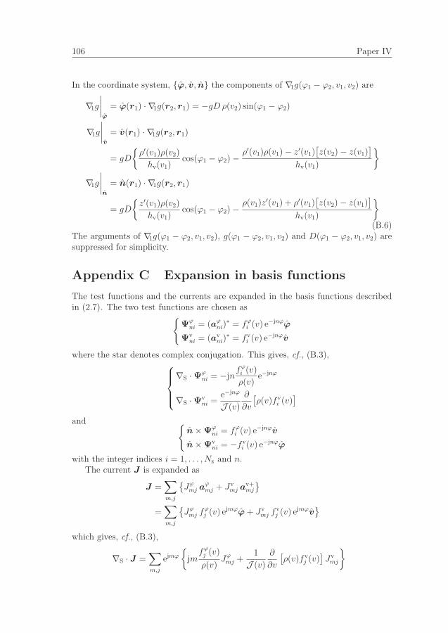
106 Paper IV

In the coordinate system, {ϕ, v, n} the components of ∇1g(ϕ1 − ϕ2, v1, v2) are

∇1g

∣∣∣∣ϕ

= ϕ(r1) · ∇1g(r2, r1) = −gD ρ(v2) sin(ϕ1 − ϕ2)

∇1g

∣∣∣∣v

= v(r1) · ∇1g(r2, r1)

= gD

{ρ′(v1)ρ(v2)

hv(v1)cos(ϕ1 − ϕ2) −

ρ′(v1)ρ(v1) − z′(v1)[z(v2) − z(v1)

]hv(v1)

}∇1g

∣∣∣∣n

= n(r1) · ∇1g(r2, r1)

= gD

{z′(v1)ρ(v2)


ρ(v1)z′(v1) + ρ′(v1)

[z(v2) − z(v1)

]hv(v1)

}(B.6)

The arguments of ∇1g(ϕ1 − ϕ2, v1, v2), g(ϕ1 − ϕ2, v1, v2) and D(ϕ1 − ϕ2, v1, v2) aresuppressed for simplicity.

Appendix C Expansion in basis functions

The test functions and the currents are expanded in the basis functions describedin (2.7). The two test functions are chosen as{

Ψϕni = (aϕ

ni)∗ = fϕ

i (v) e−jnϕϕ

Ψvni = (av

ni)∗ = fv

i (v) e−jnϕv

where the star denotes complex conjugation. This gives, cf., (B.3),⎧⎪⎪⎨⎪⎪⎩∇S · Ψϕ

ni = −jnfϕ

i (v)

ρ(v)e−jnϕ

∇S · Ψvni =

e−jnϕ

J (v)

∂

∂v

[ρ(v)fv

i (v)]

and {n × Ψϕ

ni = fϕi (v) e−jnϕv

n × Ψvni = −fv

i (v) e−jnϕϕ

with the integer indices i = 1, . . . , Nz and n.The current J is expanded as

J =∑m,j

{Jϕ

mj aϕmj + Jv

mj av+mj

}=

∑m,j

{Jϕ

mj fϕj (v) ejmϕϕ + Jv

mj fvj (v) ejmϕv

}which gives, cf., (B.3),

∇S · J =∑m,j

ejmϕ

{jmfϕ

j (v)

ρ(v)Jϕ

mj +1

J (v)

∂

∂v

[ρ(v)fv

j (v)]Jv

mj

}

D Integration over ϕ 107

andn × J =

∑m,j

{Jϕ

mj fϕj (v) ejmϕv − Jv

mj fvj (v) ejmϕϕ

}with the integer indices j = 1, . . . , Nz and m, and J

ϕ/vmj denoting the expansion

coefficients. The magnetic current M is expanded in a similar way with expansioncoefficients Mmj.

C.1 Evaluation of a cross product

In this appendix the cross product in (2.9) is evaluated, i.e.,

∇1g(r2, r1) × M(r1) = g(ϕ1 − ϕ2, v1, v2)D(ϕ1 − ϕ2, v1, v2)

·({[z′(v1)ρ(v2)


ρ(v1)z′(v1) + ρ′(v1)

[z(v2) − z(v1)

]hv(v1)

]v(ϕ1, v1)

+[−ρ

′(v1)ρ(v2)

hv(v1)cos(ϕ1 + ϕ2) +

ρ′(v1)ρ(v1) − z′(v1)[z(v2) − z(v1)

]hv(v1)

]n(ϕ1, v1)

}·∑m,j

Mϕmj f

ϕj (v1) ejmϕ1

+{[

−z′(v1)ρ(v2)

hv(v1)cos(ϕ1 − ϕ2) +

ρ(v1)z′(v1) + ρ′(v1)

[z(v2) − z(v1)

]hv(v1)

]ϕ(ϕ1)

− ρ(v2) sin(ϕ1 − ϕ2)n(ϕ1, v1)}·∑m,j

Mvmj f

vj (v1) ejmϕ1

)(C.1)

where (2.8) and (B.6) are used. The function D(ϕ1 − ϕ2, v1, v2) is labeled in (B.5).

Appendix D Integration over ϕ

The integration in the angular direction of (2.6) and (2.9) is investigated in detail.Nine different integrals Ia/A−Ii/I appear. The integrals from (2.6) and (2.9) have thesame form, but the ones in (2.6) contain singularities and are denoted by upper-caseindices. One of the integrals is studied in detail, while the others are listed at theend of this section. The cross product in (2.6) and (2.9) is evaluated separately inAppendix C.1.

The relevant integral is

Ib =

2πˆ

0

2πˆ

0

g(ϕ1 − ϕ2, v1, v2)e−jnϕ2ejmϕ1 cos(ϕ1 − ϕ2) dϕ1 dϕ2

A change of variable, ϕ1 = ϕ2 + φ, gives

Ib =

2πˆ

0

g(φ, v1, v2)ejmφ cos(φ)

2πˆ

0

ej(m−n)ϕ2 dϕ2 dφ

108 Paper IV

The inner integral is zero if m �= n. Therefore, the only interesting case is n = m,giving

Ib = 2π

2πˆ

0

g(φ, v1, v2) [cos(mφ) + j sin(mφ)] cos(φ) dφ

= 4π

πˆ

0

g(φ, v1, v2) cos(mφ) cos(φ) dφ

= 2π

πˆ

0

g(φ, v1, v2) cos([m− 1]φ) dφ+ 2π

πˆ

0

g(φ, v1, v2) cos([m+ 1]φ) cos dφ

using that g(φ, v1, v2) is an even function in φ.The rest of the integrals in the angular direction of (2.9) are derived in the same

manner and listed below.

Ia =

2πˆ

0

2πˆ

0

g(ϕ1 − ϕ2, v1, v2)ejm(ϕ1−ϕ2) dϕ1 dϕ2 = 4π

πˆ

0

g(φ, v1, v2) cos(mφ) dφ

= 4π Gm(v1, v2)

Ib =

2πˆ

0

2πˆ

0

g(ϕ1 − ϕ2, v1, v2)ejm(ϕ1−ϕ2) cos(ϕ1 − ϕ2) dϕ1 dϕ2

= 4π

πˆ

0

g(φ, v1, v2) cos(mφ) cos(φ) dφ = 2π[Gm−1(v1, v2) +Gm+1(v1, v2)

]

Ic =

2πˆ

0

2πˆ

0

g(ϕ1 − ϕ2, v1, v2)ejm(ϕ1−ϕ2) sin(ϕ1 − ϕ2) dϕ1 dϕ2

= 4πj

πˆ

0

g(φ, v1, v2) sin(mφ) sin(φ) dφ = 2πj[Gm−1(v1, v2) −Gm+1(v1, v2)

]

Id =

2πˆ

0

2πˆ

0

g(ϕ1 − ϕ2, v1, v2)D(ϕ1 − ϕ2, v1, v2)ejm(ϕ1−ϕ2) dϕ1 dϕ2

= 4π

πˆ

0

g(φ, v1, v2)D(φ, v1, v2) cos(mφ) dφ = 4π Gm(v1, v2)

Ie =

2πˆ

0

2πˆ

0

g(ϕ1 − ϕ2, v1, v2)D(ϕ1 − ϕ2, v1, v2)ejm(ϕ1−ϕ2) cos(ϕ1 − ϕ2) dϕ1 dϕ2

= 4π

πˆ

0

g(φ, v1, v2)D(φ, v1, v2) cos(mφ) cos(φ) dφ

D Integration over ϕ 109

= 2π[Gm−1(v1, v2) + Gm+1(v1, v2)

]If =

2πˆ

0

2πˆ

0

g(ϕ1 − ϕ2, v1, v2)D(ϕ1 − ϕ2, v1, v2)ejm(ϕ1−ϕ2) sin(ϕ1 − ϕ2) dϕ1 dϕ2

= 4πj

πˆ

0

g(φ, v1, v2)D(φ, v1, v2) sin(mφ) sin(φ) dφ

= 2πj[Gm−1(v1, v2) − Gm+1(v1, v2)

]Ig =

2πˆ

0

2πˆ

0

g(ϕ1 − ϕ2, v1, v2)D(ϕ1 − ϕ2, v1, v2)ejm(ϕ1−ϕ2) cos(ϕ1 − ϕ2)

· sin(ϕ1 − ϕ2) dϕ1 dϕ2

= 2πj

πˆ

0

g(φ, v1, v2)D(φ, v1, v2) sin(mφ) sin(2φ) dφ

= πj[Gm−2(v1, v2) − Gm+2(v1, v2)

]Ih =

2πˆ

0

2πˆ

0

g(ϕ1 − ϕ2, v1, v2)D(ϕ1 − ϕ2, v1, v2)ejm(ϕ1−ϕ2) cos2(ϕ1 − ϕ2) dϕ1 dϕ2

= 2π

πˆ

0

g(φ, v1, v2)D(φ, v1, v2) cos(mφ)[1 + cos(2φ)

]dφ

= 2πGm(v1, v2) + π[Gm−2(v1, v2) + Gm+2(v1, v2)

]Ii =

2πˆ

0

2πˆ

0

g(ϕ1 − ϕ2, v1, v2)D(ϕ1 − ϕ2, v1, v2)ejm(ϕ1−ϕ2) sin2(ϕ1 − ϕ2) dϕ1 dϕ2

= 2π

πˆ

0

g(φ, v1, v2)D(φ, v1, v2) cos(mφ)[1 − cos(2φ)

]dφ

= 2πGm(v1, v2) − π[Gm−2(v1, v2) + Gm+2(v1, v2)

]The new Green functions are defined as

Gm(v1, v2) =

πˆ

0


Gm(v1, v2) =

πˆ

0

g(φ, v1, v2)D(φ, v1, v2) cos(mφ) dφ

(D.1)

where φ = ϕ1 − ϕ2, the function D is defined in (B.5), and m is an integer index.Observe that these Green functions are not singular as r1 and r2 are always different.

The angular integrals of (2.6), IA − II, have the same appearance as Ia − Ii.However, the Green functions contain singularities and are denoted by gm(v1, v2)

110 Paper IV

and �m(v1, v2). The numerical treatment of these singularities is addressed in Ap-pendix E.

Appendix E Singularities in the Greens functions

Two new Greens functions, i.e.,⎧⎪⎪⎪⎪⎪⎪⎨⎪⎪⎪⎪⎪⎪⎩gm(v1, v2) =

πˆ

0


�m (v1, v2) =

πˆ

0

g(φ, v1, v2)D(φ, v1, v2) cos(mφ) dφ

are defined in the derivation of the integral equation (2.6), where g(φ, v1, v2) isdefined in (2.2), D(φ, v1, v2) in (B.5), and m is an integer index. These Green func-tions contain singularities. In this appendix, one way of handling these singularitiesis shown.

Integrals containing gm have the form˜f(v1, v2)gm(v1, v2) dv1 dv2. The inte-

grand gm(v1, v2) has a logarithmic singularity, i.e., gm(v1, v2) ∼ ln|v1 − v2|, i.e., theintegral is of the type [6] ˆ b

a

f(x) lnx dx

Changing variables x = y2gives an integral where the singularity is removed, i.e.,

ˆ √b

√a

f(y2) ln y2 2y dy

The second Green function contains a singularity of the third order, i.e.,

�m(v1, v2) =

ˆg(φ, v1, v2)D(φ, v1, v2) cos(mφ) dφ =

ˆe−jkR

[1 + jkR

]4πR3

cos(mφ) dφ

where R = |r2 − r1|. This Green function occurs in two different combinations,either as

�m−1(v1, v2) − �m+1(v1, v2)

orf(v1, v2) �m (v1, v2) + h(v1, v2) [�m−1(v1, v2) + �m+1(v1, v2)]

E Singularities in the Greens functions 111

The first combination can be rewritten as

�m−1 (v1, v2) − �m+1(v1, v2) = 2

πˆ

0

g(φ, v1, v2)D(φ, v1, v2) sin(mφ) sin(φ) dφ

=1

2π

πˆ

0

{e−jkR

R+ jk e−jkR

}sin(mφ) sin(φ)

R2︸︷︷︸singularity removed

dφ

=1

2π

πˆ

0

{ e−jkR − 1

R︸︷︷︸singularity removed

+1

R︸︷︷︸analytically solved

+ jk e−jkR}sin(mφ) sin(φ)

R2dφ

That is, the singularities are removed.The second combination is rewritten as

f(v1, v2) �m (v1, v2) + h(v1, v2) [�m−1(v1, v2) + �m+1(v1, v2)]

=

πˆ

0

g(φ, v1, v2)D(φ, v1, v2)[f(v1, v2) + h(v1, v2) cos(φ)

]cos(mφ) dφ

=

πˆ

0

1

4π

{ e−jkR − 1


+1


+ jk e−jkR}

·[f(v1, v2) + h(v1, v2) cos(φ)

][ 1

R2− 2

sin2(

mφ2

)R2︸︷︷︸

singularity removed

]dφ

Continuing with the term that still contains a singularity gives

πˆ

0

1

4π

{e−jkR − 1

R+

1

R+ jk e−jkR

}[f(v1, v2) + h(v1, v2) cos(φ)

] 1

R2dφ

=

πˆ

0

1

4π

{e−jkR − 1

R+

1

R+ jk e−jkR

}[f(v1, v2)

R2+h(v1, v2)

R2− 2h(v1, v2)

sin2(

φ2

)R2︸︷︷︸

singularity removed

]dφ

This means that the only term where the singularities are not removed so far isπ

0

g(φ, v1, v2)D(φ, v1, v2)[f(v1, v2) + h(v1, v2)] dφ. To remove this last singularity we

investigate the triple integral, i.e.,˝

. . . dφ dv1 dv2 instead of performing the in-tegrations over φ and v separately. The actual expressions of the terms containing

112 Paper IV

this last singularity are,cf., Appendix G,⎧⎪⎪⎪⎪⎪⎪⎪⎪⎪⎪⎨⎪⎪⎪⎪⎪⎪⎪⎪⎪⎪⎩

¨−ρ(v1)z

′(v2) �m (v1, v2)

+[ρ(v2)z

′(v2) − ρ′(v2)[z(v2) − z(v1)]]�m−1(v1, v2) + �m+1(v1, v2)

2dv1 dv2¨

−z′(v1)ρ(v2) �m (v1, v2)

+[ρ(v1)z

′(v1) + ρ′(v1)[z(v2) − z(v1)]]�m−1(v1, v2) + �m+1(v1, v2)

2dv1 dv2

Both integrals are treated in the same way, i.e., only the first one is investigated indetail. Only the part of the Green functions containing the singularity is investigated

¨ πˆ

0

−ρ(v1)z′(v2)g(φ, v1, v2)D(φ, v1, v2)

+[ρ(v2)z

′(v2) − ρ′(v2)[z(v2) − z(v1)]]g(φ, v1, v2)D(φ, v1, v2) dφ dv1 dv2

=

¨ πˆ

0

[z′(v2)[ρ(v2) − ρ(v1)] − ρ′(v2)[z(v2) − z(v1)]

]e−jkR[1 + jkR

]4πR3

dφ dv1 dv2

(E.1)Now, both ρ(v1) and z(v1) are expanded in its Taylor series about v1 = v2.

ρ(v1) = ρ(v2) + ρ′(v2)(v1 − v2) +ρ′′(v2)

2(v1 − v2)

2 + O((v1 − v2)3)

z(v1) = z(v2) + z′(v2)(v1 − v2) +z′′(v2)

2(v1 − v2)

2 + O((v1 − v2)3)

That is, in the vicinity of v2, (E.1) can be written as

¨ πˆ

0

[z′(v2)[−ρ′(v2)(v1 − v2) − ρ′′(v2)

2(v1 − v2)

2]

− ρ′(v2)[−z′(v2)(v1 − v2) − z′′(v2)

2(v1 − v2)

2]]e−jkR

[1 + jkR

]4πR3

dφ dv1 dv2

=1

2

¨ πˆ

0

[−z′(v2)ρ′′(v2) + ρ′(v2)z

′′(v2)](v1 − v2)

2 e−jkR[1 + jkR

]4πR3

dφ dv1 dv2

=1

8π

¨ πˆ

0

[−z′(v2)ρ′′(v2) + ρ′(v2)z

′′(v2)] (v1 − v2)

2

R2︸︷︷︸singularity removed

·{ e−jkR − 1


+1


+ jk e−jkR}

dφ dv1 dv2

and all the singularities are removed.

F Matrix formulation of the integral representation 113

Appendix F Matrix formulation of the integral

representation

In this section equation (2.9), i.e.,[vϕ

]·{−jωμ0

¨

Srad

g(r1, r2)J(r1) dS1 + j1

ωε0

¨

Srad

∇1g(r1, r2)[∇1S · J(r1)

]dS1

+

¨

Srad

∇1g(r1, r2) × M(r1) dS1

}=

[v · E(r2)ϕ · E(r2)

]=

[Ev(ϕ2, v2)Eϕ(ϕ2, v2)

]r2 ∈ Smeas

⇐⇒− jωμ0 I1 + j

1

ωε0I2 + I3 = E

is rewritten into a system of matrices. Start by writing I1, I2 and I3 as

(I1)ij = Z11aij Jv

j + Z12aij Jϕ

j

(I2)ij = Z11bij Jv

j + Z12bij Jϕ

j

(I3)ij = X11ij M

vj +X12

ij Mϕj

for the v-component and

(I1)ij = Z21aij Jv

j + Z22aij Jϕ

j

(I2)ij = Z21bij Jv

j + Z22bij Jϕ

j

(I3)ij = X21ij M

vj +X22

ij Mϕj

for the ϕ-component. The indices are j = 1, . . . , J , where J = Nz and i = 1, . . . , I,where I = Nmeas

z . This gives the matrix system,

− jωμ0 [I1] +j

ωε0[I2] + [I3] =[ −jωμ0 [Z11a] + jωε0

[Z11b

] −jωμ0 [Z12a] + jωε0

[Z12b

]−jωμ0 [Z21a] + j

ωε0

[Z21b

] −jωμ0 [Z22a] + jωε0

[Z22b

] ] [[Jv][Jϕ]

]+

[[X11] [X12][X21] [X22]

] [[Mv][Mϕ]

]=

[[Ev][Eϕ]

]⇐⇒[

[Z11] [Z12][Z21] [Z22]

] [[Jv][Jϕ]

]+

[[X11] [X12][X21] [X22]

] [[Mv][Mϕ]

]=

[[Ev][Eϕ]

](F.1)

for all m. Expressions for the matrix elements[Zkl

]and

[Xkl

]are derived in the

next section.

114 Paper IV

F.1 The impedance matrices

For a given value of the index m, the impedance matrices in (F.1) are given byZ11

ij = −jωμ0Z11aij + j

ωε0Z11b

ij where⎧⎪⎪⎪⎪⎪⎪⎪⎪⎪⎪⎪⎪⎪⎪⎨⎪⎪⎪⎪⎪⎪⎪⎪⎪⎪⎪⎪⎪⎪⎩

Z11aij =

1

hv(v2)

ˆfv

j (v1)ρ(v1){ρ′(v1)ρ

′(v2)Ib + z′(v1)z′(v2)Ia

}dv1

= 2

ˆfv

j (v1)ρ(v1)z′(v1)Gm(v1, v2) dv1

Z11bij =

1

hv(v2)

ˆ∂

∂v1

[ρ(v1)f

vj (v1)

]{ρ′(v2)ρ(v2)Ii + ρ′(v2)ρ(v2)Ih

+ z′(v2)[z(v2) − z(v1)]Id − ρ(v1)ρ′(v2)Ie

}dv1

= 2

ˆ∂

∂v1

[ρ(v1)f

vj (v1)

][z(v2) − z(v1)

]Gm(v1, v2) dv1

and Z12ij = −jωμ0Z

12aij + j

ωε0Z12b

ij where⎧⎪⎪⎪⎪⎪⎪⎪⎪⎪⎪⎨⎪⎪⎪⎪⎪⎪⎪⎪⎪⎪⎩

Z12aij = − ρ′(v2)

hv(v2)

ˆfϕ

j (v1)hv(v1)ρ(v1)Ic dv1 = 0

Z12bij = j

m

hv(v2)

ˆfϕ

j (v1)hv(v1){ρ′(v2)ρ(v2)Ii + ρ′(v2)ρ(v2)Ih

+ z′(v2)[z(v2) − z(v1)

]Id − ρ(v1)ρ

′(v2)Ie

}dv1

= 2jm

ˆfϕ

j (v1)hv(v1)[z(v2) − z(v1)

]Gm(v1, v2) dv1


21aij + j

ωε0Z21b

ij where⎧⎪⎪⎪⎪⎪⎪⎪⎪⎪⎪⎨⎪⎪⎪⎪⎪⎪⎪⎪⎪⎪⎩

Z21aij =

ˆfv

j (v1)ρ(v1)ρ′(v1)Ic dv1

= j

ˆfv

j (v1)ρ(v1)ρ′(v1)

[Gm−1(v1, v2) −Gm+1(v1, v2)

]dv1

Z21bij =

ˆρ(v1)

∂

∂v1

[ρ(v1)f

vj (v1)

]If dv1

= j

ˆρ(v1)

∂

∂v1

[ρ(v1)f

vj (v1)

][Gm−1(v1, v2) − Gm+1(v1, v2)]

dv1


22aij + j

ωε0Z22b

ij where⎧⎪⎪⎪⎪⎪⎪⎪⎪⎪⎪⎨⎪⎪⎪⎪⎪⎪⎪⎪⎪⎪⎩

Z22aij =

ˆfϕ

j (v1)hv(v1)ρ(v1)Ib dv1

=

ˆfϕ

j (v1)hv(v1)ρ(v1)[Gm−1(v1, v2) +Gm+1(v1, v2)

]dv1

Z22bij = jm

ˆfϕ

j (v1)ρ(v1)hv(v1)If dv1

= −mˆfϕ

j (v1)ρ(v1)hv(v1)[Gm−1(v1, v2) − Gm+1(v1, v2)

]dv1

F Matrix formulation of the integral representation 115

and

X11ij =

ˆfv

j (v1)ρ(v1)

hv(v2)

·[−ρ(v1)z

′(v1)ρ′(v2) − ρ′(v1)ρ

′(v2)[z(v2) − z(v1)

]+ρ′(v1)ρ(v2)z

′(v2)]If dv1

= j

ˆfv

j (v1)ρ(v1)ρ′(v1)ρ(v2)

[Gm−1(v1, v2) − Gm+1(v1, v2)]

dv1

X12ij =

1

hv(v2)

ˆfϕ

j (v1)ρ(v1)hv(v1)

(−ρ(v1)z

′(v2)Id

+[ρ(v2)z

′(v2) − ρ′(v2)[z(v2) − z(v1)]]Ie

)dv1

=

ˆfϕ

j (v1)ρ(v1)hv(v1)

(−2ρ(v1)Gm(v1, v2)

+ρ(v2)[Gm−1(v1, v2) + Gm+1(v1, v2)

])dv1

X21ij =

ˆfv

j (v1)ρ(v1)

(−z′(v1)ρ(v2)Ih +

[ρ(v1)z

′(v1) + ρ′(v1)[z(v2) − z(v1)]]Ie

− z′(v1)ρ(v2)Ii

)dv1

=

ˆfv

j (v1)ρ(v1)

(−2z′(v1)ρ(v2)Gm(v1, v2)

+[ρ(v1)z

′(v1) + ρ′(v1)[z(v2) − z(v1)]][Gm−1(v1, v2) + Gm+1(v1, v2)

])dv1

X22ij = −

ˆfϕ

j (v1)hv(v1)ρ(v1)[z(v2) − z(v1)

]If dv1

= −j

ˆfϕ

j (v1)hv(v1)ρ(v1)[z(v2) − z(v1)

][Gm−1(v1, v2) − Gm+1(v1, v2)]

dv1

where the integrals Ia − Ii are given in Appendix D and the Green functions aredefined in (D.1).

116 Paper IV

Appendix G Matrix formulation of the integral

equation

In this section equation (2.6), i.e.,

jωμ0

¨

Srad

¨

Srad

Ψ(r2) · g(r1, r2)J(r1) dS1 dS2

− j1

ωε0

¨

Srad

¨

Srad

[∇2S · Ψ(r2)]g(r1, r2)

[∇1S · J(r1)]

dS1 dS2

−¨

Srad

¨

Srad

Ψ(r2) ·[∇′g(r1, r2) × M(r1)

]dS1 dS2

− 1

2

¨

Srad

[n(r2) × Ψ(r2)

] · M(r2) dS2 = 0

⇐⇒jωμ0 I4 − j

1

ωε0I5 − I6 − 1

2I7 = 0

(G.1)

is rewritten into a system of matrices. Start by writing I4-I7 as

(I4)ij = Z11Aij Jv

j + Z12Aij Jϕ

j

(I5)ij = Z11Bij Jv

j + Z12Bij Jϕ

j

(I6)ij = X11Aij Mv

j +X12Aij Mϕ

j

(I7)ij = X11Bij Mv

j +X12Bij Mϕ

j

when Ψ = Ψvmi and

(I4)ij = Z21Aij Jv

j + Z22Aij Jϕ

j

(I5)ij = Z21Bij Jv

j + Z22Bij Jϕ

j

(I6)ij = X21Aij Mv

j +X22Aij Mϕ

j

(I7)ij = X21Bij Mv

j +X22Bij Mϕ

j

when Ψ = Ψϕmi. The indices are j = 1, . . . , J , where J = Nz and i = 1, . . . , I, where

I = Nz. This give the matrix system,

jωμ0 [I4] − j

ωε0[I5] − [I6] − 1

2[I7] =[

jωμ0

[Z11A

]− jωε0

[Z11B

]jωμ0

[Z12A

]− jωε0

[Z12B

]jωμ0

[Z21A

]− jωε0

[Z21B

]jωμ0

[Z22A

]− jωε0

[Z22B

] ] [[Jv][Jϕ]

]+

[ − [X11A

]− 12

[X11B

] − [X12A

]− 12

[X12B

]− [

X21A]− 1

2

[X21B

] − [X22A

]− 12

[X22B

] ] [[Mv][Mϕ]

]=

[[0][0]

]⇐⇒

G Matrix formulation of the integral equation 117

[[Z11] [Z12][Z21] [Z22]

] [[Jv][Jϕ]

]+

[[X 11] [X 12][X 21] [X 22]

] [[Mv][Mϕ]

]=

[[0][0]

](G.2)

for all m. Expressions for the matrix elements[Zkl

]and

[Xkl

]are derived in the

next section.

G.1 The impedance matrices

For a given value of the index m, the impedance matrices in (G.2) are given byZ11

ij = jωμ0Z11Aij − j

ωε0Z11B

ij where⎧⎪⎪⎪⎪⎪⎪⎪⎪⎪⎪⎪⎪⎪⎪⎪⎨⎪⎪⎪⎪⎪⎪⎪⎪⎪⎪⎪⎪⎪⎪⎪⎩

Z11Aij =

¨fv

i (v2)fvj (v1)ρ(v2)ρ(v1)

{ρ′(v2)ρ

′(v1) IB + z′(v1)z′(v2) IA

}dv1 dv2

= 4π

¨fv

i (v2)fvj (v1)ρ(v2)ρ(v1)

·{ρ′(v2)ρ

′(v1)gm−1 + gm+1

2+ z′(v1)z

′(v2)gm

}dv1 dv2

Z11Bij =

¨∂

∂v2

[ρ(v2)f

vi (v2)

] ∂

∂v1

[ρ(v1)f

vj (v1)

]IA dv1 dv2

= 4π

¨∂

∂v2

[ρ(v2)f

vi (v2)

] ∂

∂v1

[ρ(v1)f

vj (v1)

]gm dv1 dv2

and Z12ij = jωμ0Z

12Aij − j

ωε0Z12B

ij where⎧⎪⎪⎪⎪⎪⎪⎪⎪⎪⎪⎨⎪⎪⎪⎪⎪⎪⎪⎪⎪⎪⎩

Z12Aij = −

¨fv

i (v2)fϕj (v1)ρ

′(v2)ρ(v2)ρ(v1)hv(v1) IC dv1 dv2

= −j 4π

¨fv

i (v2)fϕj (v1)ρ

′(v2)ρ(v2)ρ(v1)hv(v1)gm−1 − gm+1

2dv1 dv2

Z12Bij = jm

¨∂

∂v2

[ρ(v2)f

vi (v2)

]fϕ

j (v1)hv(v1) IA dv1 dv2

= j 4πm

¨∂

∂v2

[ρ(v2)f

vi (v2)

]fϕ

j (v1)hv(v1)gm dv1 dv2

and Z21ij = jωμ0Z

21Aij − j

ωε0Z21B

ij where⎧⎪⎪⎪⎪⎪⎪⎪⎪⎪⎪⎨⎪⎪⎪⎪⎪⎪⎪⎪⎪⎪⎩

Z21Aij =

¨fϕ

i (v2)fvj (v1)ρ(v1)ρ

′(v1)ρ(v2)hv(v2) IC dv1 dv2

= j 4π

¨fϕ

i (v2)fvj (v1)ρ(v1)ρ

′(v1)ρ(v2)hv(v2)gm−1 − gm+1

2dv1 dv2

Z21Bij = −jm

¨fϕ

i (v2)hv(v2)∂

∂v1

[ρ(v1)f

vj (v1)

]IA dv1 dv2

= −j 4πm

¨fϕ

i (v2)hv(v2)∂

∂v1

[ρ(v1)f

vj (v1)

]gm dv1 dv2

118 Paper IV

and Z22ij = jωμ0Z

22Aij − j

ωε0Z22B

ij where⎧⎪⎪⎪⎪⎪⎪⎪⎪⎪⎪⎨⎪⎪⎪⎪⎪⎪⎪⎪⎪⎪⎩

Z22Aij =

¨fϕ

i (v2)fϕj (v1)ρ(v2)hv(v2)ρ(v1)hv(v1) IB dv1 dv2

= 4π

¨fϕ

i (v2)fϕj (v1)ρ(v2)hv(v2)ρ(v1)hv(v1)

gm−1 + gm+1

2dv1 dv2

Z22Bij = m2

¨fϕ

i (v2)fϕj (v1)hv(v2)hv(v1) IA dv1 dv2

= 4πm2

¨fϕ

i (v2)fϕj (v1)hv(v2)hv(v1) gm dv1 dv2

and X 11ij = −X11A

ij − 12X11B

ij where⎧⎪⎪⎪⎪⎪⎪⎪⎪⎪⎪⎪⎪⎪⎪⎪⎨⎪⎪⎪⎪⎪⎪⎪⎪⎪⎪⎪⎪⎪⎪⎪⎩

X11Aij =

¨fv

j (v1)fvi (v2)ρ(v1)ρ(v2)

· [−ρ(v1)z′(v1)ρ

′(v2) − ρ′(v1)ρ′(v2)

[z(v2) − z(v1)

]+ ρ′(v1)ρ(v2)z

′(v2)]IF dv1 dv2

= 4πj

¨fv

j (v1)fvi (v2)ρ(v1)ρ(v2)

·{−ρ(v1)z

′(v1)ρ′(v2) − ρ′(v1)ρ

′(v2)[z(v2) − z(v1)

]+ ρ′(v1)ρ(v2)z

′(v2)}

· �m−1(v1, v2) − �m+1(v1, v2)

2dv1 dv2

X11Bij = 0


ij − 12X12B where⎧⎪⎪⎪⎪⎪⎪⎪⎪⎪⎪⎪⎪⎪⎪⎪⎪⎨⎪⎪⎪⎪⎪⎪⎪⎪⎪⎪⎪⎪⎪⎪⎪⎪⎩

X12Aij =

¨fϕ

j (v1)fvi (v2)ρ(v1)ρ(v2)hv(v1)

(−ρ(v1)z

′(v2)ID

+[ρ(v2)z

′(v2) − ρ′(v2)[z(v2) − z(v1)]]IE

)dv1 dv2

= 4π

¨fϕ

j (v1)fvi (v2)ρ(v1)ρ(v2)hv(v1)

(−ρ(v1)z

′(v2) �m (v1, v2)

+[ρ(v2)z

′(v2) − ρ′(v2)[z(v2) − z(v1)]]�m−1(v1, v2) + �m+1(v1, v2)

2

)dv1 dv2

X12Bij = −2π

ˆfv

i (v2)fϕj (v2)ρ(v2)hv(v2) dv2

References 119


ij − 12X21B

ij where⎧⎪⎪⎪⎪⎪⎪⎪⎪⎪⎪⎪⎪⎪⎪⎪⎪⎨⎪⎪⎪⎪⎪⎪⎪⎪⎪⎪⎪⎪⎪⎪⎪⎪⎩

X21Aij =

¨fv

j (v1)fϕi (v2)ρ(v1)ρ(v2)hv(v2)

(−z′(v1)ρ(v2)IH

+[ρ(v1)z

′(v1) + ρ′(v1)[z(v2) − z(v1)]]IE − z′(v1)ρ(v2)II

)dv1 dv2

= 4π

¨fv

j (v1)fϕi (v2)ρ(v1)ρ(v2)hv(v2)

(−z′(v1)ρ(v2) �m (v1, v2)

+[ρ(v1)z

′(v1) + ρ′(v1)[z(v2) − z(v1)]]�m−1(v1, v2) + �m+1(v1, v2)

2

)dv1 dv2

X21Bij = 2π

ˆfϕ

i (v2)fvj (v2)ρ(v2)hv(v2) dv2


ij − 12X22B

ij where⎧⎪⎪⎪⎪⎪⎪⎪⎪⎨⎪⎪⎪⎪⎪⎪⎪⎪⎩

X22Aij = −

¨fϕ

j (v1)fϕi (v2)ρ(v1)ρ(v2)hv(v1)hv(v2)

[z(v2) − z(v1)

]IF dv1 dv2

= −4πj

¨fϕ

j (v1)fϕi (v2)ρ(v1)ρ(v2)hv(v1)hv(v2)

[z(v2) − z(v1)

]· �m−1(v1, v2) − �m+1(v1, v2)

2dv1 dv2

X22Bij = 0

where the integrals IA − II are given in Appendix D and the Green functions aresingular versions of the ones defined in (D.1). The numerical treatment of thesingularities in the integrals is addressed in Appendix E.

References

[1] R. A. Adams. Calculus: a complete course. Addison-Wesley, Reading, MA,USA, third edition, 1995.

[2] M. Andersson. Software for analysis of radome performance. In Proc. Interna-tional Conference on Electromagnetics in Advanced Applications (ICEAA’05),pages 537–539, Torino, Italy, 2005.

[3] R. Aster, B. Borchers, and C. Thurber. Parameter Estimation and InverseProblems. Academic Press, New York, 2005.


[5] C. A. Balanis. Advanced Engineering Electromagnetics. John Wiley & Sons,New York, 1989.

120 Paper IV

[6] A. Bondeson, T. Rylander, and P. Ingelstrom. Computational Electromagnetics.Springer-Verlag, Berlin, 2005.

[7] C. Cappellin, O. Breinbjerg, and A. Frandsen. Properties of the transformationfrom the spherical wave expansion to the plane wave expansion. Radio Sci.,43(1), 2008.

[8] C. Cappellin, A. Frandsen, and O. Breinbjerg. Application of the SWE-to-PWEantenna diagnostics technique to an offset reflector antenna. IEEE Antennasand Propagation Magazine, 50(5), 204–213, 2008.

[9] D. Colton and R. Kress. Integral Equation Methods in Scattering Theory. JohnWiley & Sons, New York, 1983.


[11] T. F. Eibert and C. H. Schmidt. Multilevel fast multipole accelerated inverseequivalent current method employing Rao-Wilton-Glisson discretization of elec-tric and magnetic surface currents. IEEE Trans. Antennas Propagat., 57(4),1178–1185, 2009.

[12] J. Friden, H. Isaksson, B. Hansson, and B. Thors. Robust phase-retrieval forquick whole-body SAR assessment using dual plane amplitude-only data. Elec-tronics Letters, 45(23), 1155–1157, 2009.

[13] M. G. Guler and E. B. Joy. High resolution spherical microwave holography.IEEE Trans. Antennas Propagat., 43(5), 464–472, 1995.



[16] D. S. Jones. Methods in Electromagnetic Wave Propagation. IEEE Press, Pis-cataway, NJ, second edition, 1994.

[17] R. E. Kleinman and G. F. Roach. Boundary integral equations for the three-dimensional Helmholtz equation. SIAM Review, 16(2), 214–236, 1974.

[18] J. A. Kong. Electromagnetic Wave Theory. John Wiley & Sons, New York,1986.

[19] D. J. Kozakoff. Analysis of Radome-Enclosed Antennas. Artech House, Boston,London, 1997.

References 121


[21] G. Kristensson. Elektromagnetisk vagutbredning. Studentlitteratur, Lund,1999. (In Swedish).

[22] F. Las-Heras, B. Galocha, and Y. Alvarez. On the sources reconstructionmethod application for array and aperture antennas diagnostics. MicrowaveOpt. Techn. Lett., 51(7), 1664–1668, 2009.

[23] F. Las-Heras, M. R. Pino, S. Loredo, Y. Alvarez, and T. K. Sarkar. Evaluatingnear-field radiation patterns of commercial antennas. IEEE Trans. AntennasPropagat., 54(8), 2198–2207, 2006.

[24] J.-J. Laurin, J.-F. Zurcher, and F. E. Gardiol. Near-field diagnostics of smallprinted antennas using the equivalent magnetic current approach. IEEE Trans.Antennas Propagat., 49(5), 814–828, 2001.


[26] E. A. Marengo and A. J. Devaney. The inverse source problem of electro-magnetics: Linear inversion formulation and minimum energy solution. IEEETrans. Antennas Propagat., 47(2), 410–412, February 1999.

[27] J. R. Mautz and R. F. Harrington. Radiation and scattering from bodies ofrevolution. Appl. Scientific Research, 20(1), 405–435, 1969.

[28] N. Morita, N. Kumagai, and J. R. Mautz. Integral Equation Methods for Elec-tromagnetics. Artech House, Boston, London, 1990.

[29] C. Muller. Foundations of the Mathematical Theory of Electromagnetic Waves.Springer-Verlag, Berlin, 1969.

[30] M. Nieto-Vesperinas. Scattering and diffraction in physical optics. World Sci-entific Publisher, Singapore, second edition, 2006.

[31] S. Nordebo, M. Gustafsson, and K. Persson. Sensitivity analysis for antennanear-field imaging. IEEE Trans. Signal Process., 55(1), 94–101, January 2007.

[32] K. Persson and M. Gustafsson. Reconstruction of equivalent currents using anear-field data transformation – with radome applications. Progress in Electro-magnetics Research, 54, 179–198, 2005.

[33] K. Persson and M. Gustafsson. Reconstruction of equivalent currents usingthe scalar surface integral representation. Technical Report LUTEDX/(TEAT-7131)/1–25/(2005), Lund University, Department of Electrical and In-formation Technology, P.O. Box 118, S-221 00 Lund, Sweden, 2005.http://www.eit.lth.se.

122 Paper IV

[34] A. F. Peterson, S. L. Ray, and R. Mittra. Computational Methods for Electro-magnetics. IEEE Press, New York, 1998.

[35] A. J. Poggio and E. K. Miller. Integral equation solutions of three-dimensionalscattering problems. In R. Mittra, editor, Computer Techniques for Electro-magnetics. Pergamon, New York, 1973.


[37] D. J. Rochblatt and B. L. Seidel. Microwave antenna holography. IEEE Trans.Microwave Theory Tech., 40(6), 1294–1300, 1992.


[39] J. A. Shifflett. CADDRAD: A physical opics radar/radome analysis code forarbitrary 3D geometries. IEEE Antennas and Propagation Magazine, 6(39),73–79, 1997.

[40] R. A. Shore and A. D. Yaghjian. Dual surface electric field integral equation.Air Force Research Laboratory Report, 2001. No. AFRL-SN-HS-TR-2001-013.

[41] R. A. Shore and A. D. Yaghjian. Dual-surface integral equations in electromag-netic scattering. IEEE Trans. Antennas Propagat., 53(5), 1706–1709, 2005.

[42] S. Silver. Microwave Antenna Theory and Design, volume 12 of RadiationLaboratory Series. McGraw-Hill, New York, 1949.

[43] J. Song and W. Chew. FMM and MLFMA in 3-D and fast Illinois solver code.In W. Chew, J.-M. Jin, E. Michielssen, and J. Song, editors, Fast and EfficientAlgorithms in Computational Electromagnetics, pages 77–118. Artech House,2001.

[44] J. C.-E. Sten and E. A. Marengo. Inverse source problem in the spheroidalgeometry: Vector formulation. IEEE Trans. Antennas Propagat., 56(4), 961–969, 2008.



References 123

[47] F. Therond, J. C. Bolomey, N. Joachmowicz, and F. Lucas. Electromagneticdiagnosis technique using spherical near-field probing. In Proc. EUROEM’94,pages 1218–1226, Bordeaux, France, 1994.

[48] J. G. van Bladel. Electromagnetic Fields. IEEE Press, New York, 2007.


[50] A. Ziyyat, L. Casavola, D. Picard, and J. C. Bolomey. Prediction of BTSantennas safety perimeter from NF to NF transformation: an experimentalvalidation. In Proc. Antenna Measurement Techniques Association (AMTA),pages 22–26, Denver, US, 2001.

Retrieval o

f equ

ivalent cu

rrents b

y the u

se of an

integ

ral represen

tation

and

the extin

ction

theo

rem —

rado

me ap

plicatio

ns Department of Electrical and Information Technology,

Faculty of Engineering, LTH, Lund University, 2010.

Retrieval of equivalent currents bythe use of an integralrepresentation and the extinctiontheorem — radome applications

Kristin Persson

Series of licentiate and doctoral theses Department of Electrical and Information Technology

1654-790X No. 22


Kristin

Persso

n

Licentiate dissertation

retrieval of equivalent currents by the use of an integral...

Documents