A&A 600, A12 (2017)DOI: 10.1051/0004-6361/201628620c© ESO 2017

Astronomy&Astrophysics

Results from a triple chord stellar occultationand far-infrared photometry of the trans-Neptunian

object (229762) 2007 UK126?,??

K. Schindler1, 2, J. Wolf1, 2, J. Bardecker3,???, A. Olsen3, T. Müller4, C. Kiss5, J. L. Ortiz6,F. Braga-Ribas7, 8, J. I. B. Camargo7, 9, D. Herald3, and A. Krabbe1

1 Deutsches SOFIA Institut, Universität Stuttgart, Pfaffenwaldring 29, 70569 Stuttgart, Germanye-mail: schindler@dsi.uni-stuttgart.de

2 SOFIA Science Center, NASA Ames Research Center, Mail Stop N211-1, Moffett Field, CA 94035, USA3 International Occultation Timing Association (IOTA), USA4 Max Planck Institute for Extraterrestrial Physics, Giessenbachstrasse 1, 85748 Garching, Germany5 Konkoly Observatory, Research Centre for Astronomy and Earth Sciences, Hungarian Academy of Sciences, Konkoly Thege 15-17,

1121 Budapest, Hungary6 Instituto de Astrofisica de Andalucia-CSIC, Glorieta de la Astronomia 3, 18080 Granada, Spain7 Observatório Nacional/MCTI, Rua Gal. José Cristino 77, 20921-400 Rio de Janeiro, Brazil8 Federal University of Technology – Paraná (UTFPR/DAFIS), Rua Sete de Setembro 3165, 80230-901 Curitiba, PR, Brazil9 Laboratório Interinstitucional de e-Astronomia – LIneA, Rua Gal. José Cristino 77, 20921-400 Rio de Janeiro, Brazil

Received 31 March 2016 / Accepted 10 October 2016

ABSTRACT

Context. A stellar occultation by a trans-Neptunian object (TNO) provides an opportunity to probe the size and shape of these distantsolar system bodies. In the past seven years, several occultations by TNOs have been observed, but mostly from a single location.Only very few TNOs have been sampled simultaneously from multiple locations. Sufficient data that enable a robust estimation ofshadow size through an ellipse fit could only be obtained for two objects.Aims. We present the first observation of an occultation by the TNO 2007 UK126 on 15 November 2014, measured by three observers,one nearly on and two almost symmetrical to the shadow’s centerline. This is the first multi-chord dataset obtained for a so-calleddetached object, a TNO subgroup with perihelion distances so large that the giant planets have likely not perturbed their orbits.We also revisit Herschel/PACS far-infrared data, applying a new reduction method to improve the accuracy of the measured fluxes.Combining both datasets allows us to comprehensively characterize 2007 UK126.Methods. We use error-in-variable regression to solve the non-linear problem of propagating timing errors into uncertainties of theellipse parameters. Based on the shadow’s size and a previously reported rotation period, we expect a shape of a Maclaurin spheroidand derive a geometrically plausible size range. To refine our size estimate of 2007 UK126, we model its thermal emission using athermophysical model code. We conduct a parametric study to predict far-infrared fluxes and compare them to the Herschel/PACSmeasurements.Results. The favorable geometry of our occultation chords, combined with minimal dead-time imaging, and precise GPS time mea-surements, allow for an accurate estimation of the shadow size (best-fitting ellipse with axes 645.80 ± 5.68 km × 597.81 ± 12.74 km)and the visual geometric albedo (pV = 15.0 ± 1.6%). By combining our analyses of the occultation and the far-infrared data, we canconstrain the effective diameter of 2007 UK126 to deff = 599−629 km. We conclude that subsolar surface temperatures are in the orderof ≈50−55 K.

Key words. Kuiper belt objects: individual: (229762) 2007 UK126 – radiation mechanisms: thermal – methods: data analysis –occultations - errata, addenda

1. Introduction

Stellar occultations are the best opportunity to directly and ac-curately determine the size and shape of a solar system body re-motely from Earth. They allow improvements of orbital elements

? Herschel is an ESA space observatory with science instruments pro-vided by European-led Principal Investigator consortia and with impor-tant participation from NASA.?? Movies are available at http://www.aanda.org

??? Also affiliated with the Western Nevada Astronomical Society,2699 Van Patten Avenue, Carson City, NV 89703, USA and the Re-search and Education Collaborative Occultation Network (RECON).

and have the potential to discover previously unknown satellites(e.g. Timerson et al. 2013; Descamps et al. 2011), or even ringsystems, as recently revealed for Centaur (10199) Chariklo(Braga-Ribas et al. 2014a). The shape of the light curve can re-veal the presence of an atmosphere, and enable the study of itsproperties (e.g. Person et al. 2013). While observations of occul-tations only require basic photometric tools, the technical chal-lenge is to acquire images at high cadence with little-to-no deadtime between acquisitions, and with very precise timing infor-mation to measure disappearance and reappearance times of theocculted star with little uncertainty. Knowledge of the target’sapparent orbital velocity and length of the occultation allow for

Open Access article, published by EDP Sciences, under the terms of the Creative Commons Attribution License (http://creativecommons.org/licenses/by/4.0),which permits unrestricted use, distribution, and reproduction in any medium, provided the original work is properly cited.

A12, page 1 of 16

A&A 600, A12 (2017)

a direct calculation of its size at the location of the sampled planeor chord. Multiple observers distributed across the shadow pathcan sample the occulting object at different locations, which pro-vides information on its shape.

Trans-Neptunian objects (TNOs) are considered the mostpristine objects in our solar system. Being left-overs from thevery early stage of the accretion phase, estimates of their sizes,densities and albedos, as well as constraints on their compositioncan provide critical information on the evolution of the solar sys-tem. Given their large geocentric distance and very small angulardiameter, the prediction of a TNO’s shadow path on the Earth’ssurface during an occultation is difficult. Owing to the very longorbital periods of TNOs, only a very small fraction of their orbitshas been observed since their discovery, leaving relatively largeuncertainties in their orbital elements. Another issue for shadowpath predictions are astrometric uncertainties of currently avail-able star catalogs, which are inherited by orbit and ephemeriscalculations for TNOs and which blur the true position of theocculted star. Besides random astrometric uncertainties that typ-ically increase towards fainter stars, catalogs usually have zonalerrors. Another dominating error that can shift a shadow pathsignificantly is potential stellar duplicity, which usually cannotbe excluded in advance. We also have no information on albedovariations on the TNO’s surface, which could cause a periodicshift of the center of light. All these error sources make pre-dictions and successful observation campaigns for TNO occul-tations a difficult task (Bosh et al. 2016). To improve shadowpath predictions, extensive astrometric observations with highprecision of both the target star and the occulting body are usu-ally conducted for many weeks in advance of an event. Thefirst data release of the Gaia star catalog (Lindegren et al. 2016;Gaia Collaboration 2016) and all subsequent data releases1 upto the final Gaia catalog in 2022 are expected to improve theaccuracy of occultation predictions significantly, since Gaia willoffer the most accurate astrometry ever obtained. Gaia will alsosignificantly contribute towards stellar duplicity measurements.

A number of occultation events covering at least 11 differ-ent TNOs (see e.g. Ortiz et al. 2014; Braga-Ribas et al. 2014b)have been successfully observed to date, not counting the well-studied Pluto system. However, most occultations by TNOscould only be observed at a single location, while the acqui-sition of multiple chords during an event has been extremelyrare. Table 1 gives an overview of all successful multi-chordobservations of occultations by TNOs (except Pluto) that havebeen published in peer-reviewed literature so far, covering onlyfour objects to date. (50000) Quaoar (Braga-Ribas et al. 2013)is currently the best sampled TNO, having five unique chords(i.e. chords that are geographically sufficiently distant to eachother to sample the occulting object at distinguishable locations)that were recorded during a single event (04 May 2011). Inthis dataset, the time resolution and accuracy of the two chordsabove the centerline have been low, resulting in large uncer-tainties of ingress and egress times and consequently in someambiguity of the ellipse fit. (136472) Makemake (Ortiz et al.2012) has been generally sampled with good time resolution,but three of the four unique chords were very close to eachother and almost located at the centerline of the ellipse fit,while the fourth chord was located below the centerline, andno chord was located above, likewise resulting in ambigu-ity of the shadow geometry. For the remaining two objects,(136199) Eris and (55636) 2002 TX300, only two unique chordsare available, which results in an under-determined ellipse fit.

1 http://www.cosmos.esa.int/web/gaia/release

To our knowledge, multi-chord events were also recorded forthe following objects, but have not been published in peer-reviewed literature so far: (208996) 2003 AZ84, (20000) Varunaand (84922) 2003 VS2.

In this paper, we report results from the very first multi-chordobservation of a stellar occultation by a TNO that is classified asa detached object according to the widely used definitions byGladman et al. (2008). This term denotes a sub class of TNOswith perihelion distances so large that Neptune and the other gi-ant planets have likely not perturbed their orbits in the past. Inaddition to being the first comprehensive study of an object ofthis dynamical class, the dataset presented in this paper is alsoextremely rare compared to previously achieved observations ofoccultations by TNOs: to our knowledge, it is only the secondafter (50000) Quaoar that provides a sufficient number of chords(at least three chords are required for an ellipse fit) that are wellspaced (in the present case sampling the target simultaneouslyabove, very close, and below the centerline by extremely fa-vorably distributed, quasi symmetrically located observers). Thesize derived from the occultation measurements is used as animportant new constraint for thermophysical modeling based onHerschel far-infrared (FIR) flux measurements. This combinedanalysis allows us to comprehensively characterize 2007 UK126.

2. Known properties of 2007 UK126 from literature

2007 UK126 was discovered at Palomar Observatory on19 October 2007. According to the database of the Minor PlanetCenter (MPC)2, it has been identified subsequently on older im-ages taken at Siding Spring Observatory and Palomar datingback to August 1982, which allowed improvements of orbit cal-culations (i = 23.34◦, e = 0.49, a = 74.01 AU). Having an or-bital period of 636.73 yr, the object is approaching perihelion (ata heliocentric distance of rH = 37.522 AU), which it will passon 18 March 2046, based on current ephemeris data providedby the JPL Small-Body Database3. Around perihelion, the targetwill have its largest apparent magnitude of mV ≈ 19.13 mag (inV-band) during its entire orbit according to MPC estimates.

Photometric and spectroscopic data of 2007 UK126 wereacquired with several instruments at ESO’s VLT in a coor-dinated campaign on 21 and 22 September 2008. Perna et al.(2010) report visible and infrared photometry (VRIJH) takenwith VLT/FORS2 and VLT/ISAAC. They estimated the abso-lute magnitude (defined as the apparent magnitude at a distanceof 1 AU both to the Sun and to the observer at zero phase an-gle) of 2007 UK126 in V-band as HV = 3.69 ± 0.04 mag. TheirR-band measurement allows us to derive HR = 3.07 ± 0.04 mag.While these photometric measurement uncertainties ∆Hphot re-sult from noise in the data, they do not consider possible peri-odic magnitude variations ∆m owing to the rotation of the body.To take these into account as well, Santos-Sanz et al. (2012) pro-posed an additional error term of ∆Hrot = 0.88 · ∆m

2 . This isjustified by assuming a sinusoidal light curve, where roughly88% of its amplitude contains 68.3% of the function values.As the light curve amplitude was not measured back in 2012,a peak-to-peak amplitude of ∆m = 0.2 mag was assumed, argu-ing that roughly 70% of a sample of TNO light curves studiedby Duffard et al. (2009) showed less magnitude variations. Con-sidering both independent error sources, the total measurement

uncertainty becomes ∆H =

√(∆Hphot

)2+ (∆Hrot)2. This leads to

2 http://www.minorplanetcenter.net3 http://ssd.jpl.nasa.gov/sbdb.cgi | http://ssd.jpl.nasa.gov/horizons.cgi

A12, page 2 of 16

K. Schindler et al.: Results from an occultation and FIR photometry of (229762) 2007 UK126

Table 1. Multi-chord observations of stellar occultations by trans-Neptunian objects (TNOs) published in peer-reviewed literature to date.

Object Dynamicalclass

Date (UTC) Location No. of recorded chords(No. of unique chords)

Keyreference

(55636) 2002 TX300 HC 09 October 2009 Hawaii 2 1(136199) Eris SDO 06 November 2010 Chile 3 (2) 2

(136472) Makemake HC 23 April 2011 Chile, Brazil 7 (4) 3(50000) Quaoar HC 04 May 2011

17 February 2012Chile, Brazil, UruguayFrance, Switzerland

6 (5)4 (2)

4

(229762) 2007 UK126 DO 15 November 2014 USA 3 this work

Notes. Numbers in brackets indicate the number of chords that were geographically sufficiently distant to each other to sample the occulting objectat distinguishable (i.e. unique) locations. Abbreviations: SDO – Scattered disk object; HC – Hot classical Kuiper belt object; DO – DetachedObject.

References. (1) Elliot et al. (2010); (2) Sicardy et al. (2011); (3) Ortiz et al. (2012); (4) Braga-Ribas et al. (2013).

refined absolute magnitude estimates of HV = 3.69 ± 0.10 magand HR = 3.07 ± 0.10 mag.

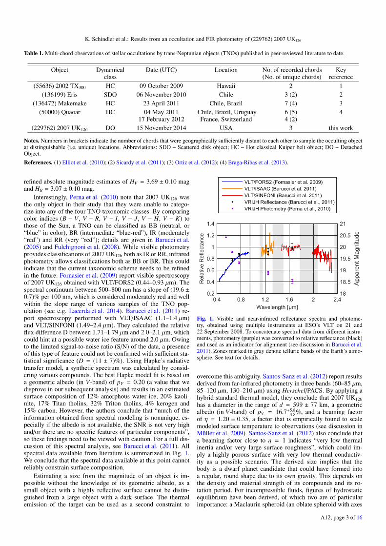
Interestingly, Perna et al. (2010) note that 2007 UK126 wasthe only object in their study that they were unable to catego-rize into any of the four TNO taxonomic classes. By comparingcolor indices (B − V , V − R, V − I, V − J, V − H, V − K) tothose of the Sun, a TNO can be classified as BB (neutral, or“blue” in color), BR (intermediate “blue-red”), IR (moderately“red”) and RR (very “red”); details are given in Barucci et al.(2005) and Fulchignoni et al. (2008). While visible photometryprovides classifications of 2007 UK126 both as IR or RR, infraredphotometry allows classifications both as BB or BR. This couldindicate that the current taxonomic scheme needs to be refinedin the future. Fornasier et al. (2009) report visible spectroscopyof 2007 UK126 obtained with VLT/FORS2 (0.44–0.93 µm). Thespectral continuum between 500–800 nm has a slope of (19.6 ±0.7)% per 100 nm, which is considered moderately red and wellwithin the slope range of various samples of the TNO pop-ulation (see e.g. Lacerda et al. 2014). Barucci et al. (2011) re-port spectroscopy performed with VLT/ISAAC (1.1–1.4 µm)and VLT/SINFONI (1.49–2.4 µm). They calculated the relativeflux difference D between 1.71–1.79 µm and 2.0–2.1 µm, whichcould hint at a possible water ice feature around 2.0 µm. Owingto the limited signal-to-noise ratio (S/N) of the data, a presenceof this type of feature could not be confirmed with sufficient sta-tistical significance (D = (11 ± 7)%). Using Hapke’s radiativetransfer model, a synthetic spectrum was calculated by consid-ering various compounds. The best Hapke model fit is based ona geometric albedo (in V-band) of pV = 0.20 (a value that wedisprove in our subsequent analysis) and results in an estimatedsurface composition of 12% amorphous water ice, 20% kaoli-nite, 17% Titan tholins, 32% Triton tholins, 4% kerogen and15% carbon. However, the authors conclude that “much of theinformation obtained from spectral modeling is nonunique, es-pecially if the albedo is not available, the SNR is not very highand/or there are no specific features of particular components”,so these findings need to be viewed with caution. For a full dis-cussion of this spectral analysis, see Barucci et al. (2011). Allspectral data available from literature is summarized in Fig. 1.We conclude that the spectral data available at this point cannotreliably constrain surface composition.

Estimating a size from the magnitude of an object is im-possible without the knowledge of its geometric albedo, as asmall object with a highly reflective surface cannot be distin-guished from a large object with a dark surface. The thermalemission of the target can be used as a second constraint to

Wavelength [µm]0.4 0.8 1.2 1.6 2 2.4

Rel

ativ

e R

eflec

tanc

e

0.2

0.4

0.6

0.8

1

1.2

1.4

VLT/FORS2 (Fornasier et al. 2009)VLT/ISAAC (Barucci et al. 2011)VLT/SINFONI (Barucci et al. 2011)VRIJH Reflectance (Barucci et al., 2011)VRIJH Photometry (Perna et al., 2010)

App

aren

t Mag

nitu

de

18

18.5

19

19.5

20

20.5

21

Fig. 1. Visible and near-infrared reflectance spectra and photome-try, obtained using multiple instruments at ESO’s VLT on 21 and22 September 2008. To concatenate spectral data from different instru-ments, photometry (purple) was converted to relative reflectance (black)and used as an indicator for alignment (see discussion in Barucci et al.2011). Zones marked in gray denote telluric bands of the Earth’s atmo-sphere. See text for details.

overcome this ambiguity. Santos-Sanz et al. (2012) report resultsderived from far-infrared photometry in three bands (60–85 µm,85–120 µm, 130–210 µm) using Herschel/PACS. By applying ahybrid standard thermal model, they conclude that 2007 UK126has a diameter in the range of d = 599 ± 77 km, a geometricalbedo (in V-band) of pV = 16.7+5.8

−3.8%, and a beaming factorof η = 1.20 ± 0.35, a factor that is empirically found to scalemodeled surface temperature to observations (see discussion inMüller et al. 2009). Santos-Sanz et al. (2012) also conclude thata beaming factor close to η = 1 indicates “very low thermalinertia and/or very large surface roughness”, which could im-ply a highly porous surface with very low thermal conductiv-ity as a possible scenario. The derived size implies that thebody is a dwarf planet candidate that could have formed intoa regular, round shape due to its own gravity. This depends onthe density and material strength of its compounds and its ro-tation period. For incompressible fluids, figures of hydrostaticequilibrium have been derived, of which two are of particularimportance: a Maclaurin spheroid (an oblate spheroid with axes

A12, page 3 of 16

A&A 600, A12 (2017)

a = b > c) and a Jacobi ellipsoid (all three axes a > b > c hav-ing different length, Chandrasekhar 1967). However, the discus-sion of these shapes only represents a theoretical limiting case,since bodies made of solid matter have mechanical strength. Aspointed out by Sheppard & Jewitt (2002), a fractured interior asa result of impacts could lead to fluid-like behavior, but condi-tions are never determined solely by hydrodynamics.

Thirouin et al. (2014) report photometric light curves takenat the Telescopio Nazionale Galileo (TNG) over a time span of≈10 h in total, distributed over three nights in October 2011.The obtained light curve of 2007 UK126 is very flat and variesby just ∆m = 0.03 ± 0.01 mag peak-to-peak. The light curveamplitude depends on the shape of the body, the viewing ge-ometry and albedo variation across the surface, all three be-ing unknown factors. Both a single-peaked (Maclaurin spheroidwith albedo inhomogeneity) and double-peaked (Jacobi ellip-soid) light curve are plausible. Thirouin et al. (2014) have useda criterion of ∆m = 0.15 mag peak-to-peak amplitude to distin-guish between albedo and shape-related light curve variations;consequently, this object was analyzed assuming a single-peaksolution. Still, they were unable to estimate a secure sidereal ro-tation period P, since data indicate multiple possible solutionsof P = {11.05 h, 14.30 h, 20.25 h}, giving the P = 11.05 h so-lution only a minimal higher likelihood compared to the othertwo. They conclude that their data only allow the rotation pe-riod to be constrained with a lower limit of P > 8 h at this time.As a rough first indicator, Thirouin et al. (2014) also derived alower density limit of ρ > 0.32 g cm−3 based on the assump-tion of a homogeneous Jacobi ellipsoid in hydrostatic equilib-rium that rotates in P = 8 h. They note that this assumption onshape is in conflict with the preference for an oblate spheroid,and emphasize that this estimate is very vague and can be un-realistic. Thirouin et al. (2014) also state an absolute magnitudeof H = 3.4 mag without specifying a filter band (presumably R)or uncertainty estimate, and indicate that no absolute photome-try has been derived; hence we discarded their value. As we nowhave additional information on the peak-to-peak amplitude of thelight curve, we can reapply the approach from Santos-Sanz et al.(2012), as explained earlier, to derive an improved uncertaintyestimate of their absolute magnitude measurements. We obtain

∆H =

√(0.04 mag

)2+

(0.88 · 0.04 mag

2

)2= 0.044 mag.

Hubble Space Telescope (HST)/WFPC2-PC observations on13 November 20084 have revealed the existence of a satellite(Noll et al. 2009; Santos-Sanz et al. 2012), but its orbit could notbe determined so far. The satellite has a magnitude differenceof ∆m = 3.79 ± 0.24 mag, measured in the HST/WFPC2-PCF606W band (599.7 nm±75 nm, see Mikulski Archive for SpaceTelescopes for more details5).

3. Observations3.1. Visual observations of the stellar occultation

2007 UK126 occulted USNO CCD Astrograph Catalog 4 starUCAC4 448-006503 in the constellation Eridanus (RAJ2000 =04h 29m 30.6s, DecJ2000 = −00◦ 28′ 20.9′′, apparent magni-tude mV = 15.86 mag (V-band), mB = 17.00 mag (B-band),mJ = 14.34 mag (J-band)6) on 15 November 2014 UTC. At

4 http://www2.lowell.edu/users/grundy/tnbs/229762_2007_UK126.html5 https://archive.stsci.edu/6 http://vizier.u-strasbg.fr/viz-bin/VizieR-5?-ref=VIZ5599d6063ad7&-out.add=.&-source=I/322A/out&UCAC4===448-006503

the time of the occultation, the target had a geocentric distanceof rG = 42.572 AU and a heliocentric distance of rH = 43.47 AU.It was close to opposition (01 December 2014, phase angleχ = 0.56) and had an approximate apparent visual magnitudeof mV ≈ 19.84 mag. Details on the prediction of this event canbe found in Camargo et al. (2014).

The event was announced in October 2014 via the RIO TNOEvents data feed7 in OccultWatcher8, a software program writ-ten by H. Pavlov (Pavlov 2014) that allows coordination amongprofessional and amateur observers, planning of campaigns, anddeployment of mobile setups across the predicted path to acquireas many chords as possible. Before the event, 25 stations regis-tered to attempt an observation of the event, while 16 stationsreported back afterwards. In addition, this event was announcedin a private email by J. L. Ortiz.

Unfortunately, weather conditions clouded out most ob-servers in California and the south western US. Three observersreported a successful observation of the event on OccultWatcher.Table 2 provides an overview of their locations and setups. Itturned out that all successful observers were coincidentally po-sitioned with almost equal spacing to each other in relation tothe shadow path, sampling the shadow almost symmetrically tothe centerline. Schindler & Wolf observed at about 89–91% hu-midity and low transparency sky conditions in California; for-tunately, the event happened during a larger gap in a high cir-rus cloud cover seen around the time of the event. The 60 cmAstronomical Telescope of the University of Stuttgart (ATUS)9,located at Sierra Remote Observatories about an hour’s drivenorth-east of Fresno, was controlled remotely from Germanyvia internet connection. Bardecker, located in Nevada, also re-ported that high cirrus clouds moved in about two minutes afterthe event. Olsen reported clear and stable weather conditions inIllinois.

Schindler & Wolf were observing with an Andor iXon DU-888 camera with a back-illuminated EMCCD sensor in2 × 2 binning mode. Being cooled to −80◦C via an internalthermo-electrical cooler, exposures are virtually free of dark cur-rent. The frame-transfer design of the EMCCD allows a fast shiftof the accumulated charge from the light-sensitive image areato a masked storage area that is read out subsequently, whilethe next exposure is already under way in the image area. Thisallows virtually gap-free imaging, with a dead time betweenframes of only 3.45 ms (the time to shift an image from the light-sensitive to the storage area). The video signal is digitized inthe camera and transmitted to a proprietary PCIe frame grabberand controller card. Image acquisition was controlled with An-dor SOLIS running on Windows 7 64 bit. Running the camerain frame-transfer mode, subsequent series of 50 frames with 2 sintegration time were taken and written directly to the PC’s harddrive into three-dimensional FITS files without buffering imagedata in the computer’s main memory (spooling). Between twoimage series, a gap of about 300 ms cannot be avoided owingto the non-real-time behavior of the operating system. A numberof 50 images per series was chosen as a compromise betweenachieving a high probability to capture the disappearance andreappearance event during an image series while still achievinga timing accuracy well below 1 ms. Precise time stamps were

7 Maintained by D. Gault, Australia, publishing predictions from theRIO TNO Group (with members from Observatório Nacional/MCTIand Observatório do Valongo/UFRJ, Rio de Janeiro, Brazil; and Ob-servatoire de Paris-Meudon/LESIA, Meudon, France).8 www.occultwatcher.com9 https://www.dsi.uni-stuttgart.de/forschung/atus.html

A12, page 4 of 16

K. Schindler et al.: Results from an occultation and FIR photometry of (229762) 2007 UK126

Table 2. Locations, setups and image acquisition parameters of successful observers, and disappearance/reappearance times derived from obtainedlight curves.

Observer Schindler & Wolf Olsen BardeckerClosest city Alder Springs, CA Urbana, IL Gardnerville, NVLatitude N (deg mm ss.ss) 37 04 13.50 40 05 12.40 38 53 23.53Longitude W (deg mm ss.ss) 119 24 45.00 88 11 46.30 119 40 20.32Altitude (m) 1405 224 1534Telescope type Ritchey-Chrétien Newtonian Schmidt-CassegrainAperture, focal ratio 600 mm, f/8 500 mm, f/4 304 mm, f/3.3Camera Andor iXon

DU-888E-C00-BVWatec 120N+ MallinCam B/W Special

Sensor type Frame transfer EMCCD(e2v CCD201-20,

back-illuminated, grade 1)

Interline transfer CCD(Sony ICX418ALL)

Interline transfer CCD(Sony ICX428ALL-A with

micro lenses)Sensor cooling (temperaturea ) Thermo-electrical (−80◦C) None (≈−9◦C) None (≈+4◦C)Frame grabber card Andor CCI-24 PCIe Pinnacle DVC-100 Hauppauge USB-Live2File format FITS, uncompressed Video, uncompressed Video, Lagarithb codecGPS time logger Spectrum Instruments TM-4,

triggered by electronicshutter of camera

Kiwi Video Time Inserter(VTI), overlaying GPS time

stamp on camera frames

IOTA Video Time Inserter(VTI), overlaying GPS time

stamp on camera framesIntegration time (s) 2.000 4.271 2.135Camera-internal frameaccumulation

none 128 × 1/29.97 64 × 1/29.97

Cycle time per frame (s) 2.00345 0.03337 0.03337Disappearance (D) time fromsquare-well fit (UTC)

10:19:24.356 ± 0.159 10:18:05.447 ± 1.032 10:19:29.151 ± 0.452

Reappearance (R) time fromsquare-well fit (UTC)

10:19:50.249 ± 0.159 10:18:26.802 ± 1.032 10:19:48.370 ± 0.452

Duration of event (s) 25.893 ± 0.225 21.355 ± 1.459 19.219 ± 0.639Chord length (km) 641.0 ± 3.9 525.9 ± 25.4 475.7 ± 11.2SNRc , star & target combined ≈12.6 ≈4.1 ≈4.7

Notes. None of the observers have used any broadband filter. (a) Given temperatures are measured at the image sensor (Schindler & Wolf) or closeto the telescope setup at the time of recording (Olsen, Bardecker). (b) Lossless video compression algorithm. (c) Signal-to-noise (S/N) ratio per datapoint.

logged with a Spectrum-Instruments TM-4 GPS receiver thatwas triggered directly via a TTL signal from the shutter portof the camera every time a series of 50 images started. Timestamps of the 2nd–50th image in a series have been extrapolatedbased on the time stamp of the first image and the well-knowncycle time. The total uncertainty of the time stamp for each ex-posure is estimated to be <0.25 ms and consists of the followingcomponents:

(a) the uncertainty of the TM-4 GPS time measurement of±10 ns (Spectrum Instruments, Inc. 2014),

(b) the synchronization of the TTL signal generated at the shut-ter port of the camera with the beginning of an exposurebetter than 1 µs (Andor Technology, priv. comm.),

(c) cycle time that is known with an accuracy of ±5 µs, whichleads to an accumulated timing uncertainty of ±245 µs afterextrapolating the time stamp for the 50th frame of a series.

Consequently, the cycle time uncertainty dominates the total un-certainty of the time measurement. The event was captured inframes 30–43 of an image series. A time-lapse animation ofthe frames acquired during the event is provided in Fig. 2 andonline. The setup was inspired by an earlier system described

by Souza et al. (2006) and is based on very good experienceswith this type of camera during characterization measurementsof the SOFIA telescope (Pfüller et al. 2012) and the subse-quent upgrade of SOFIA’s focal plane imager (Wolf et al. 2014).Differential aperture photometry was performed relative to fivefield stars in AstroImageJ10 (Collins & Kielkopf 2013; Collins2015; Collins et al. 2016), an image processing program writtenin Java on the basis of ImageJ (Schneider et al. 2012). The aper-ture radius was initially set to 3 pixels and subsequently variedbased on the estimated full width at half maximum (FWHM)of the star image (radial profile mode). The background annu-lus size was set to an inner radius of 8 and an outer radius of16 pixels; no background stars were visible within the annuli.

Olsen and Bardecker used monochrome video cameras thatemploy uncooled interline CCDs. Ambient temperature duringdata recording was −9◦C (Olsen) and +4◦C (Bardecker); sensortemperatures could not be measured and were somewhat higherthan ambient owing to heat dissipated by the camera’s sensor andelectronics. An interline CCD has a masked storage column next

10 http://www.astro.louisville.edu/software/astroimagej/

A12, page 5 of 16

A&A 600, A12 (2017)

Fig. 2. Time lapse of the stellar occultation by TNO 2007 UK126 asrecorded by Schindler & Wolf (if the animation fails to appear, clickhere), playing 10× faster than real time. The time stamp indicates thestart of each individual exposure; all frames have been cropped to210 × 210 pixels.

to each light sensitive imaging column. All accumulated chargesare simultaneously shifted sidewards into masked columns thatare read out subsequently while the next frame is already ac-quired in the light sensitive area. Thanks to this design, these im-age sensors are also virtually free of any dead time and widelyused in video cameras. The disadvantages compared to frame-transfer CCDs (that mostly find application in scientific cam-eras) are their reduced light-sensitive area and less optimizednoise characteristics. The disadvantage of a reduced fill factoris partly mitigated by the use of micro lenses that are placed oneach pixel of the CCD, which is the case in the MallinCam B/WSpecial used by Bardecker. This results in a higher sensitivitycompared to the Watec 120N+ used by Olsen that has a sensorwithout micro lenses. Both types of cameras are widely used byamateurs who routinely conduct observations of occultations andreport their results to the International Occultation Timing As-sociation (IOTA). Based on the monochrome EIA video signalstandard (Engineering Industries Association (EIA) 1957), thesecameras are running with a fixed frame rate of 29.97 frames/s(59.94 fields/s) and have an analog video output. One framehas 525 lines and consists of two fields that are interlaced (firstfield even-numbered lines, second field odd-numbered lines).To achieve longer integration times, a number of n frames can beaccumulated internally in the camera. Since the camera and itsoutput are running at a fixed frame rate, the camera provides anaccumulated frame n-times at its output, while it is accumulatingthe next frame (see Fig. 3). A video time inserter (VTI) was usedto overlay a GPS-provided time stamp on the lower part of eachfield coming from the camera’s analog video signal output. Thetime-stamped analog video signal was then digitized directly toa Windows PC via a USB video capture device by using the soft-ware VirtualDub11. Olsen captured the video into uncompressedvideo files of 4 min length, while Bardecker used the lossless La-garith video codec and recorded in segments of 5 min. The eventwas captured by both observers well within a video segment.

Data reduction differs from classical CCD imaging in twoways: the camera returns the same accumulated frame n times,superimposed with noise from analog amplifiers and the analog-digital conversion of the video capture device. This means thatthe accumulated frame is sampled n times, so the average valueof all samples in the respective bin is a representative value of

11 http://www.virtualdub.org/

the measured signal. Therefore, data have to be binned accord-ingly over n frames, corresponding to each image accumulationinterval. During data reduction, internal camera delays specificto each camera model (e.g. the accumulated image is delayed bya number of fields at the camera output) and VTI (e.g. the timestamp is delayed by a field) need to be considered to preciselyestablish the start of each individual exposure.

The captured digital video has been analyzed with Tangra 3(Pavlov 2014) and Limovie (K. Miyashita12) to extract the un-corrected time stamp for each frame from the video and toconduct differential aperture photometry of the target and fieldstars. While a classical annulus was used in Olsen’s datasetfor background estimation, two annulus sectors had to be usedin Bardecker’s dataset as a satellite trail was recorded in di-rect proximity of the target star in the frame integrated from10:19:48.370 to 10:19:50.505 UTC. This accumulated framerecorded the reappearance of the target star at Bardecker’s loca-tion; the profile of the target star could be clearly distinguishedfrom the background. The two annular sectors were carefully po-sitioned to avoid any pixels being contaminated by the satellitetrail for local background estimation. A slight contamination ofthe central aperture could not be avoided, which resulted in aslightly overestimated flux of the target star, as seen in Fig. 3 inthe first data point after the estimated end of the occultation atBardecker’s site. Usage of a classical annulus for background es-timation would have caused an overestimated background level,similar in counts to the measurement in the central aperture onthe reappearing star, thus hiding the reappearance of the starin the derived light curve, and overestimating the length of theevent at Bardecker’s location by 2.135 s.

Time stamp corrections were applied as described in George(2014) based on measurements by G. Dangl13, with the help ofthe software package R-OTE14 (George & Anderson 2013): forBardecker’s dataset, a correction of −2.1355 s accounting forcamera delay and −0.01668 s accounting for VTI delay wasmade; for Olsen’s dataset, applied corrections were −4.2876 sand −0.01668 s, respectively.

The difference in S/N between the three datasets is causedby differences in telescope aperture size, noise characteristicsof the respective camera (e.g. dark noise, amplifier noise, readnoise of A/D converters), and sensor design affecting quantumefficiency (back-illuminated frame-transfer CCD with fill fac-tor =1 vs. front-illuminated interline CCD with fill factor <1,with or without micro lenses; differences in AR coating). Giventhe small telescopes used in this campaign, the low S/N was anecessary compromise to sample the faint star at an acceptablecadence, while integration times have been chosen wisely to goto the limit of the respective equipment.

3.2. Far-infrared observations with Herschel/PACS

In addition to the data obtained from the occultation, wehave revisited far-infrared photometric data that were pre-viously acquired with the PACS photometer (Poglitsch et al.2010) on-board Herschel (Pilbratt et al. 2010). Table 3 providesa summary of all observations of 2007 UK126 that weremade on 08 and 09 August 2010. This dataset has been re-duced by constructing double-differential images optimized bysource matching, which leads to a higher S/N compared tosupersky-subtracted images used in a previous reduction by

12 http://www005.upp.so-net.ne.jp/k_miyash/occ02/limovie_en.html13 http://www.dangl.at/ausruest/vid_tim/vid_tim1.htm14 http://www.asteroidoccultation.com/observations/NA/

A12, page 6 of 16

K. Schindler et al.: Results from an occultation and FIR photometry of (229762) 2007 UK126

Table 3. Summary of observations of 2007 UK126 with Herschel/PACS.

OBSID Start time (UTC) Bands β (deg)1342202277 2010 Aug. 08 17:52:17 B/R 1101342202278 2010 Aug. 08 18:02:48 B/R 701342202279 2010 Aug. 08 18:13:19 G/R 1101342202280 2010 Aug. 08 18:23:50 G/R 701342202324 2010 Aug. 09 12:47:55 B/R 701342202325 2010 Aug. 09 12:58:26 B/R 1101342202326 2010 Aug. 09 13:08:57 G/R 1101342202327 2010 Aug. 09 13:19:28 G/R 70

Notes. OBSID denotes a Herschel internal ID for each observation. Allobservations were done in standard mini scan-map mode with a scan-leg length of 3′, a scan-leg separation of 4′′, and a total of 10 scan legs,resulting in a duration of 603 s per acquisition. For more details on themini scan-map mode, its data reduction and calibration, see Balog et al.(2014). The scan-maps were taken with the specified orientation angle βrelative to the instrument. During each observation, data were taken si-multaneously in two bands: B – blue band (60–85 µm), G – green band(85–120 µm), R – red band (130–210 µm). All observations were con-ducted with a repetition factor of 2, i.e. all maps have been observedtwice.

Santos-Sanz et al. (2012). Also, the PACS pipeline flux calibra-tion is based on standard stars and asteroids that are significantlybrighter than the target. The absolute photometric calibration ofour reduction is instead based on a number of faint standardstar measurements. The applied data reduction technique is de-scribed in detail in Kiss et al. (2014). The fluxes obtained in eachband are summarized in Table 4.

We have also checked data from the Wide-field Infrared Sur-vey Explorer (WISE, Wright et al. 2010) satellite for possibledetections of 2007 UK126. Although two possible detections inimages taken on 10 January 2010 are listed in the WISE All-Sky Known Solar System Object Possible Association List15, weconcluded that those are false positives for several reasons: theassociated sources are off by several arcsec from their predictedpositions, and our thermophysical modeling (see Sect. 5) pre-dicts fluxes in the WISE bands that are well below the respectivedetection limits. Both Herschel/PACS and WISE measurementswere taken close in time, i.e. at very similar observing geometry,so it appears safe to say that 2007 UK126 was below the detectionlimits of WISE. Also, the Minor Planet Center does not list anyentries for 2007 UK126 reported from WISE.

4. Results from the stellar occultation

4.1. Occultation light curves and square-well fits

The integration time and achieved S/N of each camera dictate thefundamental limit of how accurate the moment of disappearanceand reappearance of the occulted star can be determined on eachchord. The expected light curve resembles a square-well if thefollowing conditions are fulfilled:

1. The body has no atmosphere, or one that is so thin that itcannot be detected, given the sampling rate and S/N.

2. Effects of Fresnel diffraction and the finite stellar diameterare negligible.

15 http://irsa.ipac.caltech.edu/cgi-bin/Gator/nph-scan?submit=Select&projshort=WISE

Considering the peak sensitivity wavelength of the Si-basedCCD cameras (λ ≈ 650 nm) and the geocentric distance of2007 UK126, the Fresnel scale is F ≈ 1.44 km (Roques et al.1987). The estimated angular stellar diameter is about 0′′.0097(van Belle 1999), or 0.3 km projected at the geocentric distanceof 2007 UK126. Given the very high speed of the shadow on theEarth’s surface of about v = 24.1 km s−1 and the three orders ofmagnitude larger size of 2007 UK126, it becomes clear that botheffects can be neglected for the dataset at hand.

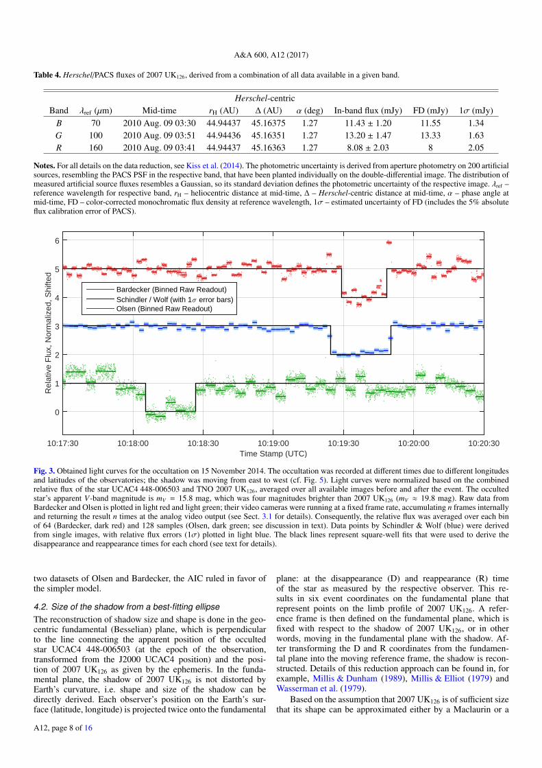
The light curves that have been obtained by the three ob-servers are illustrated in Fig. 3, together with derived square-well fits. All relative fluxes have been normalized based on theaverage combined relative flux of star and TNO in all availableexposures before and after the occultation (“baseline”). Noneof the light curves indicate a gradual decline and emergenceof the star, so a square-well fit is a legitimate approximation.Given the achieved sampling rates, the presence of a thin at-mosphere cannot be excluded; this question remains to be stud-ied during future occultations that allow for faster sampling (i.e.brighter star or availability of larger telescopes). Given the quasi-zero dead time of all cameras used in this study, disappear-ance and reappearance of the occulted star must have occurred(with near-100% certainty) during integration of an exposure (asingle frame for Schindler/Wolf, or n accumulated frames forBardecker and Olsen). The measured relative flux in the respec-tive exposure is consequently smaller than the combined relativeflux of the star and the TNO, but larger than the TNO’s relativeflux alone.

The S/N of the dataset of Schindler & Wolf is sufficientto clearly isolate the frames that recorded disappearance andreappearance, and to interpolate their time stamps to subframeaccuracy. As the response of the CCD is linear, the ratio be-tween the measured relative flux in the disappearance or reap-pearance frame and the baseline is directly proportional to theoffset of disappearance or reappearance in time relative to thestart of the respective exposure16. An upper and lower limit ofthis ratio has been derived using the normalized relative flux er-ror σSignal = (S/N)−1, which propagates directly into the un-certainty of the estimated disappearance and reappearance timesσD/R = σSignal tint, as given in Table 2.

Unfortunately, the S/Ns of the datasets of Olsen andBardecker do not allow for the identification of the accumu-lated frame that recorded disappearance and reappearance. Thisbecomes clear from the light curves: none of the accumulatedframes has a relative flux that separates it from the upper orlower baseline with statistical significance. Thus, we decidedto apply square-well fits that are coincident with the samplingfrequency. Again, the normalized relative flux error has beenused as an uncertainty estimate to calculate timing uncertain-ties (see Table 2). We note that the R-OTE software packageuses the Akaike information criterion (AIC) as a logic to de-cide objectively if a square-well fit shall be applied to exposuretiming (3 parameter model) or sub-exposure timing (4 param-eter model). While the goodness of fit improves with an addi-tional parameter, the fit is not necessarily a better representationof the data at hand. By weighing the number of parametersof a model against its goodness of fit, AIC provides a formalway to decide if sub-exposure timing can be applied. For the

16 This simplification is only accurate for a body without any atmo-sphere. Assuming a gradual dimming would have happened on shortertime scales than the integration time, the gradual transition could havebeen integrated by a single image. The length of the chord would thenbe slightly overestimated.

A12, page 7 of 16

A&A 600, A12 (2017)

Table 4. Herschel/PACS fluxes of 2007 UK126, derived from a combination of all data available in a given band.

Herschel-centricBand λref (µm) Mid-time rH (AU) ∆ (AU) α (deg) In-band flux (mJy) FD (mJy) 1σ (mJy)

B 70 2010 Aug. 09 03:30 44.94437 45.16375 1.27 11.43 ± 1.20 11.55 1.34G 100 2010 Aug. 09 03:51 44.94436 45.16351 1.27 13.20 ± 1.47 13.33 1.63R 160 2010 Aug. 09 03:41 44.94437 45.16363 1.27 8.08 ± 2.03 8 2.05

Notes. For all details on the data reduction, see Kiss et al. (2014). The photometric uncertainty is derived from aperture photometry on 200 artificialsources, resembling the PACS PSF in the respective band, that have been planted individually on the double-differential image. The distribution ofmeasured artificial source fluxes resembles a Gaussian, so its standard deviation defines the photometric uncertainty of the respective image. λref –reference wavelength for respective band, rH – heliocentric distance at mid-time, ∆ – Herschel-centric distance at mid-time, α – phase angle atmid-time, FD – color-corrected monochromatic flux density at reference wavelength, 1σ – estimated uncertainty of FD (includes the 5% absoluteflux calibration error of PACS).

Time Stamp (UTC)10:17:30 10:18:00 10:18:30 10:19:00 10:19:30 10:20:00 10:20:30

Rel

ativ

e F

lux,

Nor

mal

ized

, Shi

fted

0

1

2

3

4

5

6

Bardecker (Binned Raw Readout)Schindler / Wolf (with 1< error bars)Olsen (Binned Raw Readout)

Fig. 3. Obtained light curves for the occultation on 15 November 2014. The occultation was recorded at different times due to different longitudesand latitudes of the observatories; the shadow was moving from east to west (cf. Fig. 5). Light curves were normalized based on the combinedrelative flux of the star UCAC4 448-006503 and TNO 2007 UK126, averaged over all available images before and after the event. The occultedstar’s apparent V-band magnitude is mV = 15.8 mag, which was four magnitudes brighter than 2007 UK126 (mV ≈ 19.8 mag). Raw data fromBardecker and Olsen is plotted in light red and light green; their video cameras were running at a fixed frame rate, accumulating n frames internallyand returning the result n times at the analog video output (see Sect. 3.1 for details). Consequently, the relative flux was averaged over each binof 64 (Bardecker, dark red) and 128 samples (Olsen, dark green; see discussion in text). Data points by Schindler & Wolf (blue) were derivedfrom single images, with relative flux errors (1σ) plotted in light blue. The black lines represent square-well fits that were used to derive thedisappearance and reappearance times for each chord (see text for details).

two datasets of Olsen and Bardecker, the AIC ruled in favor ofthe simpler model.

4.2. Size of the shadow from a best-fitting ellipseThe reconstruction of shadow size and shape is done in the geo-centric fundamental (Besselian) plane, which is perpendicularto the line connecting the apparent position of the occultedstar UCAC4 448-006503 (at the epoch of the observation,transformed from the J2000 UCAC4 position) and the posi-tion of 2007 UK126 as given by the ephemeris. In the funda-mental plane, the shadow of 2007 UK126 is not distorted byEarth’s curvature, i.e. shape and size of the shadow can bedirectly derived. Each observer’s position on the Earth’s sur-face (latitude, longitude) is projected twice onto the fundamental

plane: at the disappearance (D) and reappearance (R) timeof the star as measured by the respective observer. This re-sults in six event coordinates on the fundamental plane thatrepresent points on the limb profile of 2007 UK126. A refer-ence frame is then defined on the fundamental plane, which isfixed with respect to the shadow of 2007 UK126, or in otherwords, moving in the fundamental plane with the shadow. Af-ter transforming the D and R coordinates from the fundamen-tal plane into the moving reference frame, the shadow is recon-structed. Details of this reduction approach can be found in, forexample, Millis & Dunham (1989), Millis & Elliot (1979) andWasserman et al. (1979).

Based on the assumption that 2007 UK126 is of sufficient sizethat its shape can be approximated either by a Maclaurin or a

A12, page 8 of 16

K. Schindler et al.: Results from an occultation and FIR photometry of (229762) 2007 UK126

Jacobi ellipsoid, its projected shadow on the Earth’s surface isexpected to be an ellipse. For a subsequent analysis of size andshape, we need to find the ellipse that best fits to the measureddisappearance (D) and reappearance (R) times (or respectively,the D and R coordinates in the reference frame moving with theshadow). An ellipse can be described by five geometrical param-eters: its center coordinates xEl, yEl, the major and minor axes aEland bEl, and the orientation angle of the major axis θEl. Fortu-nately, the availability of three chords covering both sides of theshadow path allows for an ellipse fit without taking additionalassumptions.

We used Occult17, a software program written and contin-uously developed by D. Herald and used by occultation ob-servers worldwide for predictions of events and subsequent dataanalysis. Using Occult, we translated measured D and R timesand their derived uncertainties (see previous section) into D andR coordinates with propagated uncertainties in the moving ref-erence frame, and calculated an initial ellipse fit (for details, seeHerald 2016). To verify these results independently, we recalcu-lated the ellipse fit with our own code written in Matlab and re-alized that the algorithm implemented in Occult has a significantshortcoming. Occult uses a direct least-square ellipse fit algo-rithm, where uncertainties of D and R timings have no effect onthe resulting ellipse and are not propagated into the uncertaintiesassociated to the ellipse parameters. Timing error estimates arecollected merely for archiving purposes at this moment. The un-certainties of the geometric ellipse parameters provided by Oc-cult are solely derived from the residuals between the ellipse andeach D or R coordinate, measured along the line between ellipsecenter and D or R. Although Occult allows the user to specifyweights to differentiate between different levels of data quality,these weights only influence the estimated uncertainties of theellipse parameters, not the ellipse fit itself.

It became clear that the desired propagation of timing errorsinto the ellipse fit leads to a non-linear errors-in-variable prob-lem. We found a perfectly suited algorithm recently describedby Szpak et al. (2015) that offers a solution for exactly this typeof problem. The D and R uncertainties can be described as inde-pendent Gaussian noise with zero mean that is inhomogeneous,i.e. that depends on the respective setup, integration time andobserving conditions. Therefore, we can use the propagated Dand R uncertainties in the moving reference frame to define acovariance matrix for each D and R coordinate. The algorithmuses these covariance matrices as weights in a cost function thatneeds to be minimized to determine the best-fitting ellipse. Afterthe algorithm has calculated the algebraic parameters of the el-lipse and their corresponding covariances, a conversion and co-variance propagation to the ellipse’s geometrically meaningfulparameters is conducted. In this way, we get a reliable and ro-bust estimate of the uncertainties of all parameters of interest,while the ellipse fit itself considers the noise in the data points.Finally, a confidence region in the plane of the ellipse is calcu-lated, illustrating the zone in which the true ellipse is located ata given probability. We chose a planar 68.3% confidence regionto be consistent with other literature in the field instead of the95% region suggested by Szpak et al. (2015), e.g. for industrialmachine vision applications.

The resulting geometrical parameters of the best fitting el-lipse and their associated uncertainties are listed in Table 5.The ellipse fit and its 68.3% confidence region is illustrated inFig. 4. The positive y axis is directed to the north, while the pos-itive x axis indicates east. The origin (x, y) = (0, 0) represents

17 http://www.lunar-occultations.com/iota/occult4.htm

Table 5. Geometric parameters of the best fitting ellipse and associateduncertainties.

Parameter ValueaEl (km) 645.80 ± 5.68bEl (km) 597.81 ± 12.74xEl (km) 6.57 ± 2.06yEl (km) −10.82 ± 3.13θEl (deg) 21.25 ± 5.65

Fig. 4. The derived ellipse fit and its 68.3% confidence region (gray).Uncertainties of each individual ellipse parameter are summarized inTable 5. The angle θ gives the rotation of the major axes, measuredfrom east to north. The plotted error bars of the D and R locations havebeen derived from the timing deviations given in Table 2. The majorand minor axes are indicated by the dotted lines. The distances providedin the legend are topocentric with respect to the centerline derived forthe best fit (dash-dotted line). The chord by Schindler & Wolf sampled2007 UK126 almost at the centerline, while the chords by Bardeckerand Olsen sampled the upper and lower part quasi symmetrically. Thegeocentric distance of 2007 UK126 was rG = 42.572 AU at the time ofthe observation.

the average of the minimum and maximum event coordinate innorth-south and east-west direction.

Figure 5 illustrates the reconstructed shadow path on the sur-face of the Earth, where the shadow’s upper and lower bound-ary and centerline are based on the size and orientation ofthe ellipse as illustrated in Fig. 4. An animation that illus-trates the shadow traveling across the continental US and themeasurements conducted in parallel is available online. We con-clude that the relative measurement uncertainty of the ellipseaxes is in the order of 0.9% and 2.1%, respectively. The axial

A12, page 9 of 16

A&A 600, A12 (2017)

21

3

1 = Bardecker2 = Schindler3 = Olsen

Fig. 5. Reconstructed shadow path and geographic locations of all ob-servers across the continental US. The three lines indicate the shadowpath’s northern boundary, centerline, and southern boundary, assumingan elliptical shape for 2007 UK126 based on the ellipse fit presented inFig. 4. The arrows indicate the direction of travel of the shadow on theEarth’s surface from east to west. An animation illustrating the eventand the acquired light curves is available online.

ratio of the ellipse translates to aEl/bEl = 1.080 ± 0.025, i.e. acircular fit and hence a pole-on viewing geometry can alreadybe ruled out geometrically.

4.3. Albedo

Thanks to the occultation measurement, we can improve the ge-ometric albedo estimate. Following the formula

pV = 4 × 100.4(HV,Sun−HV,TNO) · (1 AU)2 a−1El b−1

El , (1)

where HV,Sun = −26.78 mag is the absolute magnitude of theSun (Bessel V18), HV,TNO = 3.69 ± 0.044 mag is the absolutemagnitude of 2007 UK126 in V-Band (see Sect. 2, although thisvalue might include a small flux contribution from a potentialsatellite) and 1 AU = 1.49598 × 108 km. Considering propaga-tion of all measurement errors (see Appendix B), we derive pV =15.0 ± 1.6%. This calculation assumes that, between the epochsof the photometric measurements (September 2008) and the oc-cultation (November 2014), the projected area did not change,i.e. the pole orientation of the body as seen from Earth remainsvirtually the same. This assumption is reasonable: as pointed outby Sheppard & Jewitt (2002), with reference to Harris (1994),an object of the size of 2007 UK126 has a damping timescalefor its non-principal axis rotation (“wobble”) that is significantlysmaller than the age of the solar system. Considering the orbitalperiod of 636.73 yr, a body in pure principal axis rotation wouldappear in almost the same projection on such short timescales.The new albedo estimate is within the previously derived rangeby Santos-Sanz et al. (2012) of pV = 16.7+5.8

−3.8%.2007 UK126 is one of eight detached objects that have been

observed with Herschel in the far-infrared and subsequentlyanalyzed via thermophysical modeling. Based on this sample,Lacerda et al. (2014) derived a median albedo for detached ob-jects of pV,DO = 16.7%. Considering our new estimate, the me-dian albedo for this class of objects shifts to pV,DO = 15.0%, butthe sample size is too small for reliable statistical analysis.

Substituting the magnitudes in Eq. (1) with the R-bandestimates HR,TNO = 3.07 ± 0.044 mag (see Sect. 2) andHR,Sun = −27.12 mag (Bessel R18), we obtain a geometric albedoin the R-band of pR = 19.5 ± 2.0%.

18 Willmer (2006), http://mips.as.arizona.edu/~cnaw/sun.html, using Bohlin & Gilliland (2004) and Fukugita et al. (1995).

4.4. Shape and size

The very small light curve variations (∆mV = 0.03 ± 0.01 magpeak-to-peak, see Sect. 2) are another strong indicator of aMaclaurin spheroid with albedo variations that is not seen pole-on. From spacecraft fly-bys, we know about objects in the so-lar system that were shaped into oblate spheroids by their owngravity, but which are considerably smaller than 2007 UK126:the icy Saturnian satellites Mimas (ρ = 1.149 ± 0.007 g cm−3,deq = 396.4 ± 0.8 km, Roatsch et al. 2009), Enceladus (ρ =

1.609 ± 0.005 g cm−3, deq = 504.2 km, Roatsch et al. 2009)and Miranda (ρ = 1.20 ± 0.14 g cm−3, deq = 472 ± 3 km,Jacobson et al. 1992). We feel it is a reasonable assumption toconstrain our following analysis to a Maclaurin spheroid thatrotates around its principal axis c, and to discard the Jacobisolution.

Viewing a Maclaurin spheroid pole-on (θ = 0◦) would leadto a circular shadow during an occultation, while viewing itequator-on (θ = 90◦) would lead directly to the elliptical shadowthat was measured. While a circular fit (and hence a pole-onview) has been ruled out geometrically, the ellipse derived inthe previous section represents a distorted projection of the trueshape of 2007 UK126 in any other pole orientation than equator-on. For a Maclaurin spheroid, we can calculate the flattening ra-tio a/c from the major axis aEl and minor axis bEl of the shadowellipse and the angle θ between the spheroid’s rotation axis andthe line of sight:

ac

=

√√√√ sin2 θb2

Ela2

El− cos2 θ

· (2)

We do not know θ at the time of the occultation. This implies thatwe can only specify a plausible range of flattening ratios basedon the uncertainties of the shadow ellipse parameters and an arbi-trary tilt angle. The upper limit of the flattening ratio is given bythe bifurcation point between a Maclaurin spheroid and a Jacobiellipsoid at a/c = 1.71609, corresponding to an ellipse eccentric-ity of e = 0.81267 (Chandrasekhar 1967). As illustrated in Fig. 6and summarized in Table 6, the flattening ratio of 2007 UK126,and therefore its size, are relatively poorly constrained.

We also do not have a density estimate for 2007 UK126.Models of volatile retention (see e.g. Schaller & Brown 2007)could be used to derive a lower bulk density limit when surfaceices or a thin atmosphere are present, but the featureless near-infrared spectrum (see Sect. 2) does not indicate the presence ofany prominent volatiles (within the S/N limits of the dataset).As pointed out by Brown (2013a), the absence of volatiles and ameasurable atmosphere cannot be used as an argument to derivean upper density limit, as Jeans escape is unfortunately not theonly mechanism that can cause a body to lose its volatiles, eventhough it is the slowest.

One way to estimate a lower bulk density limit would bea precise determination of the rotation period. At bifurcation,we can calculate the density of the spheroid as shown byChandrasekhar (1967) from

ρ =ω2

0.37423 π G, (3)

where ω denotes the angular velocity and G = 6.67384 ×10−11 m3 kg−1 s−2 the gravitational constant. We only know that2007 UK126 takes more than P > 8 h for a full rotation (seeSect. 2), which means its bulk density at bifurcation would be

A12, page 10 of 16

K. Schindler et al.: Results from an occultation and FIR photometry of (229762) 2007 UK126

Tilt angle of principal axis c [deg]0 15 30 45 60 75 90

Sph

eroi

d fla

tteni

ng ra

tio a

/c

1

1.25

1.5

1.75

2

Best fitting ellipse axes ratio (aEl /bEl = 1.080)

Confidence interval for best fitting ellipse axes ratioBifurcation point (a/c = 1.716)Limit for 0.73 g cm-3 , P > 8 h (a/c 1.487)Possible solutionsPossible solutions with constraint 0.73 g cm-3, P > 8 h

Fig. 6. Flattening ratio a/c of the Maclaurin spheroid as a function ofangle θ between the spheroid’s rotation axis and the line of sight. With-out a density estimate, true flattening ratios up to the bifurcation pointare theoretically plausible. We argue that a more realistic lower densitylimit is ρ = 0.73 g cm−3, which would exclude extreme axis ratios andtherefore constrain the volume of the body considerably.

ρ < 0.61 g cm−3. Rotation period and density are indirectly pro-portional to the square, i.e. if the body takes twice as long for afull rotation, its lower density limit would be one quarter of thisestimate. We can therefore not constrain a lower limit on bulkdensity for 2007 UK126 at this time.

Estimated bulk densities and sizes of TNOs have been col-lected, e.g. in Ortiz et al. (2012) (see supplementary informa-tion), Brown (2013b) and Johnston (2014). We compiled a listof all TNOs whose size has been constrained by thermophysi-cal modeling and/or occultations, and bulk density has been es-timated owing to the presence of a satellite with a known or-bit (see Appendix A). We did not include TNOs for which bulkdensity estimates have been derived solely from light curves (asan assumption on body figure has to be made in these cases),or limits on bulk density have been stated mistakenly based onthe absence of volatiles or a measurable atmosphere. Our listcovers 19 objects with a diameter range of 157−2374 km. Weemphasize that this compilation can only be used for qualitativestatements; it is not meaningful to derive a correlation functionbetween size and density – the sample is too small, could be ob-servationally biased, and uncertainties are, in general, very large.Also, the large diversity among the TNO population is not under-stood, and bodies could have undergone entirely different evo-lutions. To our knowledge, no density estimate has been derivedfor any detached object to date. Only few objects have been stud-ied through far-infrared observations, and 2007 UK126 is the firstdetached object that has been studied in detail during an occul-tation. In addition, the limits of orbital elements of the detachedobject population are unclear, and transitional objects betweenthe scattered disk and the inner Oort cloud could belong to thispopulation as well. The only two scattered disk objects (SDOs)for which densities have been estimated thanks to their satellitesare Ceto (dsystem,eff = 281 ± 11 km, ρ = 0.64+0.16

−0.13 g cm−3, pV =5.6±0.6, Santos-Sanz et al. 2012) and Eris (deff = 2326±12 km,ρ = 2.52 ± 0.05 g cm−3, pV = 96+9

−4%, Sicardy et al. 2011). Bothobjects could not be more contrary in character; their properties

Table 6. Possible size range of the axes of a Maclaurin spheroid.

Parameter a/c < 1.7161 a/c ≤ 1.4870P ≥ 8 h

ρ ≥ 0.73 g cm−3

a = b (km) 640−651 640−651c (km) 373−611 432−611

dSphere,eff (km) 535−638 563−638

Notes. The equivalent diameter of a sphere dSphere has been calculatedto compare with a previous size estimate.

are at complete opposite ends of the parameter space, illustratingthe difficulties at hand.

From our list, we find that, except for two targets (both abouthalf the size of 2007 UK126), no TNO has an estimated densityρ < 0.6 g cm−3. This corresponds to our estimated lower densitylimit at bifurcation based on P = 8 h. A subset of 13 objects inour list have a size deff < 800 km; the average density of thissubset is ρ̄ = 0.87 g cm−3, while the median density is ρmedian =0.73 g cm−3. Eleven of these 13 objects are smaller than deff <400 km, so this selection is strongly biased towards objects thatare significantly smaller than 2007 UK126.

We feel that it is unlikely that 2007 UK126 has a bulk densitybelow ρ = 0.73 g cm−3 given its size, since this would require asignificant porosity comparable to a comet. The Rosetta missionrevealed a density of ρ = 0.533 ± 0.006 g cm−3 and a poros-ity of 72−74% for the nucleus of 67P/Churyumov-Gerasimenko(Pätzold et al. 2016). These properties appear feasible for highlyfractured rubble piles, but are hard to imagine for a dwarf planetcandidate that is larger than the three Saturnian satellites men-tioned earlier. Arguing from a different perspective, finding anoblate spheroid with a flattening ratio close to bifurcation isvery unlikely, since 2007 UK126 is certainly not composed ofa strengthless fluid. Solving the following equation provided byChandrasekhar (1967) numerically,

ρ = ω2

π G

√1 − e2

e3 2(3 − 2e2

)arcsin e −

6e2

(1 − e2

)−1

, (4)

leads to an ellipse eccentricity of e = 0.7401, or a/c = 1.4870,assuming ρ = 0.73 g cm−3 and P = 8 h. A longer rotation periodwould lower the flattening ratio. We feel that a flattening ratio ofa/c = 1.4870 represents an acceptable, albeit qualitative, upperlimit.

Table 6 summarizes the possible size range of all threespheroid axes for both the generic case (unknown density) andconsidering the added qualitative constraint on density. It can beseen that the occultation data is able to improve the previous sizeestimate of dSphere,eff = 599±77 km for an equivalent sphere thatwas derived by Santos-Sanz et al. (2012) solely through thermo-physical modeling based on Herschel/PACS data. In the nextsection, we refine our size estimate from the occultation furtherthrough thermophysical modeling, using the occultation data asconstraints.

5. Results from thermophysical modeling

To improve our geometrically obtained size estimate of2007 UK126, we model the body’s thermal emission using a ther-mophysical model (TPM) code. We conduct a parametric study

A12, page 11 of 16

A&A 600, A12 (2017)

to predict far-infrared fluxes for a wide range of plausible ge-ometries and physical properties, and compare them to our re-reduced Herschel/PACS measurements presented in Sect. 3.2.A description of the thermophysical model, its parameters andfurther details can be found in Müller & Lagerros (1998, 2002).The model considers the heliocentric distance of 2007 UK126(rH = 44.944 AU) at the epoch of Herschel’s observations.

2007 UK126 is considered a binary system. Since we do notknow the position of the satellite relative to the primary duringHerschel’s observations, we need to consider that the satellitemight have contributed some flux to the Herschel/PACS mea-surements. We therefore studied the following cases to constrainwhich combination of parameters are compatible to the occulta-tion and to the Herschel/PACS data:

I the satellite did not contribute flux to the observed FIRfluxes;

II the satellite contributed a maximum plausible flux to theobserved FIR fluxes;

each considering

(a) a thermal inertia ofΓ = {0.3, 0.7, 1, 3, 5, 10} J m−2 s−0.5 K−1;

(b) a surface roughness with a slope of s = {0.1, 0.5, 0.9} rms;(c) a rotation period of P = {8, 11.05, 14.30, 20.25} h

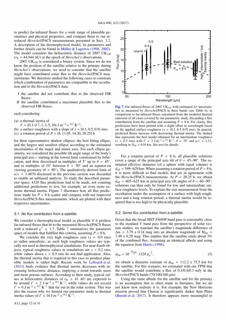
for three representative shadow ellipses: the best fitting ellipse,and the largest and smallest ellipse according to the estimateduncertainties of the major and minor axes. For each ellipse ge-ometry, we considered the possible tilt angle range of the body’sprincipal axis c starting at the lowest limit constrained by bifur-cation, and then discretized in multiples of 5◦ up to θ = 45◦,and in multiples of 10◦ between θ = 50◦ and an equator-onviewing geometry (θ = 90◦). The qualitatively derived limit ofa/c = 1.4870 discussed in the previous section was discardedto enable an unbiased analysis. To study the described param-eter space, 4320 flux predictions had to be made, not countingadditional predictions to test, for example, an even more ex-treme thermal inertia. Figure 7 illustrates how all flux predic-tions made for P = 8 h scatter and compare with our improvedHerschel/PACS flux measurements, which are plotted with theirrespective uncertainties.

5.1. No flux contribution from a satellite

We consider a thermophysical model as plausible if it predictsfar-infrared fluxes that fit to the measured Herschel/PACS fluxeswith a reduced χ2 ≤ 1.7. Table 7 summarizes the parameterspace of models that fulfilled this criteria, assuming P = 8 h.

We consider the very high roughness case (s = 0.9 rms)as rather unrealistic, as such high roughness values are typi-cally not used in thermophysical simulations. For near-Earth ob-jects, typical roughness values in simulations are s = 0.2 rms,while values above s > 0.5 rms do not find application. Also,the thermal inertia that is required in this case to produce plau-sible models is rather high. Recent work by Lellouch et al.(2013) finds evidence that thermal inertia decreases with in-creasing heliocentric distance, implying a trend towards moreand more porous surfaces. According to their study, typical val-ues at heliocentric distances of rH > 41 AU are expected tobe around Γ ≈ 2 J m−2 s−0.5 K−1, while values do not exceedΓ ≈ 6 J m−2 s−0.5 K−1 that far out in the solar system. This wasalso the reason why we limited our parameter study to thermalinertia values of Γ ≤ 10 J m−2 s−0.5 K−1.

100Wavelength [µm]

0

5

10

15

20

25

Best solution

Psid = 8 h

rms=0.1

0.5

0.9

20050

hig

h /

inte

rme

dia

te /

low

the

rma

l in

ert

ia

Flu

x [m

Jy]

Fig. 7. Far-infrared fluxes of 2007 UK126 with estimated 1σ uncertain-ties as measured by Herschel/PACS in three bands (see Table 4), incomparison to far-infrared fluxes calculated from the modeled thermalemission of all cases covered by our parametric study, discarding a fluxcontribution from the satellite and assuming P = 8 h. For clarity, fluxpredictions have been plotted with a slight offset in wavelength basedon the applied surface roughness (s = {0.1, 0.5, 0.9} rms). In general,predicted fluxes increase with decreasing thermal inertia. The dashedline represents the best model obtained for an intermediate roughness(s = 0.5 rms) with Γ = 3 J m−2 s−0.5 K−1, θ = 70◦ and a/c = 1.11,resulting in Deff = 618 km. See text for details.

For a rotation period of P = 8 h, all plausible solutionscover a range of the principal axis tilt of θ = 45−90◦. The es-timated effective diameter (of a sphere with equal volume) isdeff = 599−629 km. When assuming a rotation period of P > 8 h,it is more difficult to find models that are in agreement withthe Herschel/PACS measurements. At P = 20.25 h, we obtaindeff = 605−625 km at principal axis tilt angles of θ = 60−90◦;solutions can then only be found for low and intermediate sur-face roughness levels. To explain the size measurement from theoccultation under the assumption of a surface with high rough-ness and a long rotation period, a thermal inertia would be re-quired that is too high to be physically plausible.

5.2. Some flux contribution from a satellite

Given that the broad HST F606W band pass is reasonably closeto the standard V band pass from the perspective of solar sys-tem studies, we translate the satellite’s magnitude difference of∆m = 3.79 ± 0.24 mag into an absolute magnitude of HSat =7.48 ± 0.29 mag. This implies that the satellite emits about 3%of the combined flux. Assuming an identical albedo and usingthe equation from Harris (1998),

dSat = 10−HV,Sat

5 1329 p−12

V , (5)

we obtain a diameter estimate of dSat = 112.2 ± 75.5 km forthe satellite. For this scenario, we estimated with our TPM thatthe satellite would contribute a flux of 0.3/0.4/0.3 mJy in theHerschel/PACS bands (70/100/160 µm).

Using the same albedo for the satellite and for the primaryis an assumption that is often made in literature, but we donot know how realistic it is. For example, the New Horizonsmission proved that Charon is significantly darker than Pluto(Buratti et al. 2017). It therefore appears more meaningful to

A12, page 12 of 16

K. Schindler et al.: Results from an occultation and FIR photometry of (229762) 2007 UK126

Table 7. Results from a parametric study with a TPM code, assuming a rotation period of P = 8 h and no flux contribution from the satellite.

Parameter Very low roughness Intermediate roughness Very high roughness(0.1 rms) (0.5 rms) (0.9 rms)

θ (degrees) 45−90 60−70 60−90Γ (J m−2 s−0.5 K−1) 0.7−10 3−10 3−10

a = b (km) 640−646 640−646 640c (km) 524−598 565−591 565−585

a/c 1.08−1.22 1.09−1.13 1.09−1.13dSphere,eff (km) 599−629 614−627 614−621

reduced χ2 1.40−1.63 1.42−1.70 1.46−1.66

study a worst case scenario for the satellite: we assume that itsalbedo is lower than for the primary (pV,Sat = 5%) and that itsbrightness is at the upper uncertainty limit of the available mea-surements (HV,Sat = 7.19 mag), implying an equivalent diameterof dSat = 217 km. Using our TPM, we estimate that this type ofsatellite produces 1.6/1.8/1.3 mJy (corresponding to ≈14−16%flux) in the Herschel/PACS bands if we use typical simulationparameters: an equator-on viewing geometry, a P = 8 h rota-tion period (assuming a tidally locked motion), a low thermalinertia of Γ = 1 J m−2 s−0.5 K−1, and an intermediate level ofsurface roughness of s = 0.5 rms. Acting as a comparison, theNEATM model (Harris 1998) produces consistent flux estimatesof 1.6/1.9/1.5 mJy for such a satellite using a beaming param-eter of η = 1.2. Subtracting the satellite’s worst-case flux esti-mates from the measured Herschel/PACS fluxes provided earlierin Table 4 gives us a minimum flux estimate of 9.9/11.5/6.7 mJyfor 2007 UK126.

Thermophysical modeling considering a satellite flux contri-bution did not lead to meaningful results at any studied rotationperiod: Although predicted fluxes typically match measurementsin the 70 µm and 100 µm bands well, they poorly fit the measure-ments in the 160 µm band. This is indicated by a much degradedreduced χ2 ≥ 3.32. Table 8 lists the range of possible propertiesof 2007 UK126 according to models with a goodness of fit in therange of 3.32 ≤ χ2 ≤ 4.0. Again, a very high roughness and avery high thermal inertia are rather unrealistic.

Given the very poor fit of our modeled fluxes to Her-schel/PACS measurements, it is very likely that the flux contri-bution from the satellite is much less than the derived worst-casecontribution, indicating that the discussion in Sect. 5.1 is a real-istic approximation.

5.3. Implications

The TPM simulations enable us to constrain the parameter spacemarked in Fig. 6 significantly. Figure 8 illustrates the surfacetemperature distribution on 2007 UK126, as predicted by theTPM for one of the best model fits: a viewing geometry ofθ = 70◦ of an oblate sphere with an effective diameter ofdeff = 618 km, a flattening ratio of a/c = 1.11, a thermal in-ertia of Γ = 3 J m−2 s−0.5 K−1, an intermediate level of surfaceroughness of s = 0.5 rms, and a rotation period of P = 8 h.This fit results in a reduced χ2 = 1.43 and predicted fluxes of10.98/13.28/10.29 mJy in Herschel’s 70/100/160 µm bands.

In our range of plausible model fits, we find maximum sur-face temperatures of about ≈50−55 K in the subsolar point.Since 2007 UK126 is still on its way to perihelion in 2046, itspends a large fraction of its orbit at comparable or even highersurface temperatures. From two perspectives, it is unlikely that

Fig. 8. Surface temperature distribution on 2007 UK126, as predictedby the TPM for the best model with an intermediate roughness (seeFig. 7 and text for details). The TPM takes the epoch of the Herschelobservation into account.

2007 UK126 has retained volatile ices (CH4, N2, and CO): be-cause of its estimated temperature levels and its small size.At the given surface temperatures, all volatiles would be lostsolely based on Jeans escape, as indicated by a greatly simpli-fied model by Schaller & Brown (2007). However, as discussedby Stern & Trafton (2008), an atmosphere on a body as small as2007 UK126 would be governed by hydrodynamic escape (ow-ing to the body’s low gravity, even considering moderate to highdensities), or by a combination of Jeans and hydrodynamic es-cape. It is unlikely that Jeans escape alone, the slowest lossmechanism, is depleting the atmosphere. Given the eccentric-ity of the orbit of 2007 UK126, the proportion of each escapemechanism could vary over time, and seasonal freeze out andsublimation of volatile ices could play a role. In addition to clas-sic escape mechanisms, impacts that almost certainly occurredthroughout the lifetime of the solar system would accelerate theescape of an atmosphere. The lack of volatiles is supported byavailable near-infrared spectra (see Sect. 2) that could not iden-tify any ice features (within the S/N limits of the dataset). How-ever, small amounts of involatile amorphous water ice, belowthe detection limit of the available spectra, cannot be excludedsince they could have been preserved at the calculated surfacetemperatures. Since no volatiles, and hence no atmosphere areexpected on 2007 UK126, the approach of fitting square-well pro-files to the occultation light curve data as discussed in Sect. 4.1is reconfirmed.

6. Conclusions

For the first time, it was possible to measure the size of a de-tached object of the TNO population directly during a stellar

A12, page 13 of 16

A&A 600, A12 (2017)

Table 8. Results from a parametric study with a TPM code, considering a maximum plausible flux contribution from the satellite and assuming arotation period of P = 8 h for the primary body.

Parameter Very low roughness Intermediate roughness Very high roughness(0.1 rms) (0.5 rms) (0.9 rms)

θ (degrees) 50−70 70−90 80−90Γ (J m−2 s−0.5 K−1) 3−10 5−10 10

a/c 1.09−1.18 1.07−1.11 1.09−1.10dSphere,eff (km) 606−627 618−637 621

reduced χ2 3.43−3.87 3.32−4.00 3.47−3.56

occultation at three locations. Our findings from the occultationmeasurements are:

1. The shadow ellipse that fits best to the times of disappear-ance and reappearance on each chord has a major axis ofaEl = 645.80 ± 5.68 km and a minor axis of bEl = 597.81 ±12.74 km (aEl/bEl = 1.080 ± 0.025).

2. The estimated projected area, combined with previous pho-tometric measurements, suggests an albedo estimate of pV =15.0± 1.6%. This estimate is consistent with and more accu-rate than an earlier estimate that was based on a size derivedsolely from a thermophysical model.

3. Owing to the very low light curve amplitude and rotation pe-riod reported in literature and the size estimated from the oc-cultation, we assume by analogy to other solar system bodiesthat 2007 UK126 resembles an oblate spheroid.

4. Given the shadow ellipse geometry and the non-zero lightcurve amplitude, 2007 UK126 was not seen pole-on.

5. We cannot constrain a bulk density at this time. Purely bygeometric means, we can constrain the effective diameter of2007 UK126 to deff = 535−638 km. We argue qualitativelythat the spheroid’s flattening ratio is likely a/c ≤ 1.4870,which would constrain the effective diameter range slightlymore to deff = 563−638 km.

6. No secondary occultation has been detected, so the satellitecould not be reobserved (although chances would have beenextremely small). This implies that it was either behind orin front of the primary, not in the primary’s shadow path, orso small that its shadow moved in between the observers’locations. With sufficient distance to the primary at the timeof the occultation, the shadow of the secondary may not haveeven hit the Earth’s surface.

Modeling the thermal emission of 2007 UK126, using geomet-rical constraints obtained from the occultation, and comparingmodeled fluxes with improved Herschel/PACS far-infrared fluxmeasurements, we conclude that:

1. The effective diameter of 2007 UK126 is likely of the orderof deff = 599−629 km. The flattening ratio is of the order ofa/c = 1.08−1.22.

2. The body was likely seen near an equator-on viewing geom-etry (θ = 45−90◦).

3. Assuming an albedo of 5% for the satellite and a worst-casephotometric error, its effective diameter would be 217 km,from which we derive the worst-case satellite flux contribu-tion in the Herschel/PACS bands. Considering a flux contri-bution from the satellite, it was not possible to derive modelsat any given rotation period that would be compatible withthe occultation shadow size and Herschel/PACS measure-ments, so it is very likely that any satellite flux contributionswould be much less.

4. Our models result in maximum surface temperatures of≈50−55 K in the subsolar point.

Combining our analyses of the occultation and the thermal emis-sion, we conclude:

1. While a true flattening ratio close to bifurcation cannot for-mally be ruled out from the occultation data, given the un-known density, high flattening ratios can be ruled out thanksto our thermal simulations. This constrains the size of thebody considerably.

2. Owing to its estimated surface temperature levels and itssmall size, it is unlikely that 2007 UK126 has retained volatileices (CH4, N2, and CO), which is also supported by its fea-tureless near-infrared spectra reported in literature. This re-confirms fitting square-well profiles to the occultation lightcurve, as no atmosphere is expected.

The estimated size supports the status of 2007 UK126 as a dwarfplanet candidate. While faster sampling of an occultation wouldhelp to decrease the uncertainties of the shadow ellipse fit, itwould not help to significantly constrain the tilt angle θ of therotation axis, which is the dominating source of uncertainty for ageometrically derived size estimate. Without a density estimate,only the observation of multiple occultations, extensive lightcurve measurements, and work on a shape model could even-tually provide better geometrical constraints on the body’s truesize. Thermophysical modeling allows to overcome this issue.Future occultations of 2007 UK126 or acquisition of additionalhigh-resolution image data will hopefully provide opportunitiesto reobserve its satellite. Knowledge of the satellite’s size andorbit is crucial to constrain the system mass and bulk density,which would immediately constrain plausible shapes. While sizeand albedo estimates solely derived from far-infrared measure-ments still have considerable uncertainties, the combined anal-ysis of occultation observations and far-infrared measurementsis a powerful tool to thoroughly characterize bodies in our solarsystem.

Acknowledgements. For their efforts on long-term occultation predictions andupdates, we thank B. Sicardy (LESIA, Observatoire de Paris), J. Desmars (IM-CEE, Paris), N. Morales, P. Santos-Sanz, R. Duffard (Instituto de Astrofisica deAndalucia-CSIC) and the following members from the Rio Group: R. Vieira-Martins, M. Assafin, A. Dias-Oliveira, B. Morgado, G. Benedetti-Rossi andA. Ramos Gomes Jr.. We would like to thank M. Hümmer for his work on creat-ing a video sequence via ray tracing illustrating the occultation based on the re-constructed geometry of 2007 UK126 (see online). K.S. has been supported finan-cially by a one-year fellowship from the German Academic Exchange Service(DAAD) during his stay at NASA Ames Research Center, CA as part of his Ph.D.research. K.S. would also like to thank the Universities Space Research Associ-ation (USRA) for their support throughout his thesis. T.M., C.K. and J.L.O. havereceived funding from the European Union’s Horizon 2020 Research and In-novation Programme, under Grant Agreement No. 687378. C.K. has been sup-ported by the PECS grant # 4000109997/13/NL/KML of the Hungarian SpaceOffice and the European Space Agency, the K-104607 grant of the Hungar-ian Research Fund (OTKA), and the GINOP-2.3.2-15-2016-00003 grant of the

A12, page 14 of 16

K. Schindler et al.: Results from an occultation and FIR photometry of (229762) 2007 UK126

National Research, Development and Innovation Office of Hungary (NKFIH).J.L.O. acknowledges support from Proyecto de Excelencia J.A. 2012-FQM1776.The Astronomical Telescope of the University Stuttgart (ATUS) has been fundedin parts by the German Aerospace Center (DLR). K.S. and J.W. would like tothank all involved parties at Sierra Remote Observatories (SRO) for providingand maintaining the infrastructure that allows us to remotely operate ATUS.L. Van Vleet was manually monitoring and controlling the observatory roof thatnight which allowed us to conduct this observation despite of critical humiditylevels. K.S. thanks T. George and R. L. Anderson, the developers of R-OTE, forvivid discussions on statistical methods and camera- and VTI-specific time offsetcorrections. This research has made use of NASA’s Astrophysics Data System.

ReferencesBalog, Z., Müller, T., Nielbock, M., et al. 2014, Exp. Astron., 37, 129Barucci, M. A., Belskaya, I. N., Fulchignoni, M., & Birlan, M. 2005, AJ, 130,

1291Barucci, M. A., Alvarez-Candal, A., Merlin, F., et al. 2011, Icarus, 214, 297Bohlin, R. C., & Gilliland, R. L. 2004, AJ, 127, 3508Bosh, A. S., Person, M. J., Zuluaga, C. A., et al. 2016, Icarus, submittedBraga-Ribas, F., Sicardy, B., Ortiz, J. L., et al. 2013, ApJ, 773, 26Braga-Ribas, F., Sicardy, B., Ortiz, J. L., et al. 2014a, Nature, 508, 72Braga-Ribas, F., Vieira-Martins, R., Assafin, M., et al. 2014b, in Rev. Mex.

Astron. Astrofis. Conf. Ser., 44, 3Brown, M. E. 2013a, ApJ, 767, L7Brown, M. E. 2013b, ApJ, 778, L34Buratti, B. J., Hofgartner, J. D., Hicks, M. D., et al. 2017, Icarus, 287, 207Camargo, J. I. B., Vieira-Martins, R., Assafin, M., et al. 2014, A&A, 561, A37Chandrasekhar, S. 1967, Comm. Pure Appl. Math., 20, 251Collins, K. A. 2015, Ph.D. Thesis, University of LouisvilleCollins, K., & Kielkopf, J. 2013, Astrophysics Source Code Library

[record ascl:1309.001]Collins, K. A., Kielkopf, J. F., & Stassun, K. G. 2016, ArXiv e-prints

[arXiv:1601.02622]Descamps, P., Marchis, F., Berthier, J., et al. 2011, Icarus, 211, 1022Duffard, R., Ortiz, J. L., Thirouin, A., Santos-Sanz, P., & Morales, N. 2009,

A&A, 505, 1283Elliot, J. L., Person, M. J., Zuluaga, C. A., et al. 2010, Nature, 465, 897Engineering Industries Association (EIA) 1957, Standard RS 170, Electrical

Performance Standards – Monochrome Television Studio FacilitiesFornasier, S., Barucci, M. A., de Bergh, C., et al. 2009, A&A, 508, 457Fornasier, S., Lellouch, E., Müller, T., et al. 2013, A&A, 555, A15Fukugita, M., Shimasaku, K., & Ichikawa, T. 1995, PASP, 107, 945Fulchignoni, M., Belskaya, I., Barucci, M. A., de Sanctis, M. C., &

Doressoundiram, A. 2008, in The Solar System Beyond Neptune, eds. M. A.Barucci, H. Boehnhardt, D. P. Cruikshank, A. Morbidelli, & R. Dotson (TheUniversity of Arizona Press), 181

Gaia Collaboration (Brown, A. G. A., et al.) 2016, A&A, 595, A2George, T. 2014, Analysis of Camera Delay Corrections for use in R-OTE and

Occular Occultation Timing Extraction Programs, White PaperGeorge, T., & Anderson, R. L. 2013, in 2013 IOTA Annual Meeting, Toronto,

CanadaGladman, B., Marsden, B. G., & Vanlaerhoven, C. 2008, in The Solar System

Beyond Neptune, eds. M. A. Barucci, H. Boehnhardt, D. P. Cruikshank,A. Morbidelli, & R. Dotson (The University of Arizona Press), 43

Harris, A. W. 1994, Icarus, 107, 209Harris, A. W. 1998, Icarus, 131, 291Herald, D. 2016, Occult v4 HelpJacobson, R. A., Campbell, J. K., Taylor, A. H., & Synnott, S. P. 1992, AJ, 103,

2068

Johnston, W. R. 2014, TNO and Centaur Diameters, Albedo, and Densities V2.0,EAR-A-COMPIL-5-TNOCENALB-V2.0, NASA Planetary Data System

Kiss, C., Müller, T., Vilenius, E., et al. 2014, Exp. Astron., 37, 161Lacerda, P., Fornasier, S., Lellouch, E., et al. 2014, ApJ, 793, L2Lellouch, E., Santos-Sanz, P., Lacerda, P., et al. 2013, A&A, 557, A60Lindegren, L., Lammers, U., Bastian, U., et al. 2016, A&A, 595, A4Millis, R. L., & Dunham, D. W. 1989, in Asteroid II, eds. R. P. Binzel, T. Gehrels,

& M. S. Matthews (University of Arizona Press), 148Millis, R. L., & Elliot, J. L. 1979, in Asteroids, ed. T. Gehrels (University of

Arizona Press), 98Mommert, M., Harris, A. W., Kiss, C., et al. 2012, A&A, 541, A93Müller, T. G., & Lagerros, J. S. V. 1998, A&A, 338, 340Müller, T. G., & Lagerros, J. S. V. 2002, A&A, 381, 324Müller, T. G., Lellouch, E., Böhnhardt, H., et al. 2009, Earth, Moon, and Planets,

105, 209Noll, K. S., Grundy, W. M., Benecchi, S. D., Levison, H. F., & Barker, E. A.

2009, in AAS/Division for Planetary Sciences Meeting Abstracts, 41, 47.07Ortiz, J. L., Sicardy, B., Braga-Ribas, F., et al. 2012, Nature, 491, 566Ortiz, J. L., Sicardy, B., Braga-Ribas, F., et al. 2014, in European Planetary

Science Congress 2014, EPSC Abstracts, 9, 525Pätzold, M., Andert, T., Hahn, M., et al. 2016, Nature, 530, 63Pavlov, H. 2014, in Eighth Trans-Tasman Symposium on Occultations (TTSO8),

Melbourne, AustraliaPerna, D., Barucci, M. A., Fornasier, S., et al. 2010, A&A, 510, A53Person, M. J., Dunham, E. W., Bosh, A. S., et al. 2013, AJ, 146, 83Pfüller, E., Wolf, J., Hall, H., & Röser, H.-P. 2012, Proc. SPIE, 8444, 844413Pilbratt, G. L., Riedinger, J. R., Passvogel, T., et al. 2010, A&A, 518, L1Poglitsch, A., Waelkens, C., Geis, N., et al. 2010, A&A, 518, L2Roatsch, T., Jaumann, R., Stephan, K., & Thomas, P. 2009, in Saturn

from Cassini-Huygens, eds. M. Dougherty, L. Esposito, & S. Krimigis(Netherlands: Springer), 763

Roques, F., Moncuquet, M., & Sicardy, B. 1987, AJ, 93, 1549Santos-Sanz, P., Lellouch, E., Fornasier, S., et al. 2012, A&A, 541, A92Schaller, E. L., & Brown, M. E. 2007, ApJ, 659, L61Schneider, C. A., Rasband, W. S., & Eliceiri, K. W. 2012, Nature Methods, 9,

671Sheppard, S. S., & Jewitt, D. C. 2002, AJ, 124, 1757Sicardy, B., Ortiz, J. L., Assafin, M., et al. 2011, Nature, 478, 493Souza, S. P., Babcock, B. A., Pasachoff, J. M., et al. 2006, PASP, 118, 1550Spectrum Instruments, Inc. 2014, Intelligent Reference/TM-4TM GPS Time &

Frequency System – User ManualSpencer, J. R., Stansberry, J. A., Grundy, W. M., & Noll, K. S. 2006, in

AAS/Division for Planetary Sciences Meeting Abstracts, 38, 546Stansberry, J., Grundy, W., Brown, M., et al. 2008, in The Solar System Beyond

Neptune, eds. M. A. Barucci, H. Boehnhardt, D. P. Cruikshank, A. Morbidelli,& R. Dotson (The University of Arizona Press), 161

Stansberry, J., Grundy, W., Mueller, M., et al. 2012, Icarus, 219, 676Stern, S. A., & Trafton, L. M. 2008, in The Solar System Beyond Neptune, eds.

M. A. Barucci, H. Boehnhardt, D. P. Cruikshank, A. Morbidelli, & R. Dotson(The University of Arizona Press), 365

Stern, S. A., Bagenal, F., Ennico, K., et al. 2015, Science, 350, 1815Szpak, Z. L., Chojnacki, W., & van den Hengel, A. 2015, J. Math. Imaging

Vision, 52, 173Thirouin, A., Noll, K. S., Ortiz, J. L., & Morales, N. 2014, A&A, 569, A3Timerson, B., Brooks, J., Conard, S., et al. 2013, Planet. Space Sci., 87, 78van Belle, G. T. 1999, PASP, 111, 1515Vilenius, E., Kiss, C., Mommert, M., et al. 2012, A&A, 541, A94Vilenius, E., Kiss, C., Müller, T., et al. 2014, A&A, 564, A35Wasserman, L. H., Millis, R. L., Franz, O. G., et al. 1979, AJ, 84, 259Wolf, J., Wiedemann, M., Pfüller, E., et al. 2014, Proc. SPIE, 9145, 91450Wright, E. L., Eisenhardt, P. R. M., Mainzer, A. K., et al. 2010, AJ, 140, 1868

A12, page 15 of 16

A&A 600, A12 (2017)

Appendix A: Density estimates

Table A.1 summarizes all TNOs for which a density estimatecould be derived to this date. The size and mass of Pluto and itssatellite Charon were measured during the New Horizons flyby.All remaining objects are binary systems, which allowed an esti-mate of the respective system mass based on the satellite’s orbit.Only the size of Eris and Quaoar have been probed through ob-servations of stellar occultations so far. All other size estimateswere derived from thermophysical modeling of Spitzer and/orHerschel data.

Appendix B: Error propagation

Applying the laws of error propagation, the error of the albedoestimate can be calculated as follows:

∆p =

( dpdHSun

∆HSun

)2

+

(dp

dHTNO∆HTNO

)2

+

(dp

daEl∆aEl

)2

+

(dp

dbEl∆bEl

)21/2

. (B.1)

In our calculations we assumed ∆HSun = 0. The remaining dif-ferentials are

dpdHTNO

=4 × (1 AU)2

aElbEl100.4HSun ln 10 × 10−0.4HTNO (B.2)

dpdaEl

= −4 × 100.4(HSun−HTNO) · (1 AU)2

a2ElbEl

(B.3)

dpdbEl

= −4 × 100.4(HSun−HTNO) · (1 AU)2

aElb2El

· (B.4)

Table A.1. Summary of TNOs with estimated bulk densities.

Target Effective diameter (km) Bulk density (g cm−3) Source(134340) Pluto 2374 ± 8 1.860 ± 0.013 Stern et al. (2015)(136199) Eris 2326 ± 12 2.52 ± 0.05 Sicardy et al. (2011)

(134340) I Charon 1212 ± 6 1.702 ± 0.021 Stern et al. (2015)(50000) Quaoar 1110 ± 5 1.99 ± 0.46 Braga-Ribas et al. (2013)(90482) Orcusa 958.4 ± 22.9 1.53+0.15

−0.13 Fornasier et al. (2013)(120347) Salaciaa 901 ± 45 1.29+0.29

−0.23 Fornasier et al. (2013)(174567) Vardaa 792+91

−84 1.27+0.41−0.44 Vilenius et al. (2014)

(55637) 2002 UX25a 692 ± 23 0.82 ± 0.11 Brown (2013b)

(47171) 1999 TC36a 393.1+25.2

−26.8 0.64+0.15−0.11 Mommert et al. (2012)

(79360) Sila-Nunama 343 ± 42 0.73 ± 0.28 Vilenius et al. (2012)(148780) Altjiraa 331+51

−187 0.30+0.50−0.14 Vilenius et al. (2014)

2001 QC298a 303+27

−30 1.14+0.34−0.30 Vilenius et al. (2014)

(26308) 1998 SM165a 279.8+29.7

−28.6 0.51+0.29−0.14 Stansberry et al. (2008), Spencer et al. (2006)

(65489) Cetoa 281 ± 11 0.64+0.16−0.13 Santos-Sanz et al. (2012)

(275809) 2001 QY297a 229+22

−108 0.92+1.30−0.27 Vilenius et al. (2014)

2001 XR254a 221+41

−71 1.00+0.96−0.56 Vilenius et al. (2014)

(88611) Teharonhiawakoa 220+41−44 0.60+0.36

−0.33 Vilenius et al. (2014)(66652) Borasisia 163+32

−66 2.1+2.60−1.2 Vilenius et al. (2014)

(42355) Typhona 157 ± 34 0.60+0.72−0.29 Stansberry et al. (2012)

Notes. (a) Binary system properties; primary not individually measured through occultation or spacecraft encounter.

A12, page 16 of 16