results applied differential/algebraic systems*

SIAM J. NUMER. ANAL.Vol. 23, No. 4, August 1986

(C) 1986 Society for Industrial and Applied Mathematics010

ORDER RESULTS FOR IMPLICIT RUNGE-KUTI’A METHODS APPLIED TODIFFERENTIAL/ALGEBRAIC SYSTEMS*

L. R. PETZOLDf

Abstract. In this paper we study the order, stability and convergence properties of implicit Runge-Kuttamethods applied to a relatively simple class of nonlinear differential/algebraic systems. These methods oftendo not attain the same order of accuracy for differential/algebraic systems as they do for purely differentialsystems. We derive a set of order conditions which the method coefficients should satisfy in addition to theusual order conditions to ensure a given order of accuracy, and we present results on the stability andconvergence properties of these methods.

Key words, differential/algebraic equations, stiff equations, Runge-Kutta methods

AMS(MOS) subject classification. 65L05

1. Introduction. In this paper we study the order, stability and convergence proper-ties of implicit Runge-Kutta methods applied to systems of differential/algebraicequations (DAE) of the form

(1.1) O=F(t,y,y’)

where the initial values of y are given at 0 and F is linear is y’. These methodsoften do not attain the same order of accuracy for differential/algebraic systems asthey do for purely differential systems. We derive a set of order conditions which themethod coefficients must satisfy in addition to the usual order conditions to ensure agiven order of accuracy of the local truncation error. Also, we present results on thestability properties and order of convergence of the global error of these methods.Finally, we describe some numerical experiments which are in agreement with ourresults.

An M-stage implicit Runge-Kutta method for the solution of a system of ordinarydifferential equations (ODEs)

(1.2) y’ =f(t, y)

is given by

(1.3)( M

Y[=f tn+c,h, yn_l+h , aijYj=l

M

yn=y,,_l+h biY,i=1

i=1,2,...,M,

where h t, in-1. The method is often written in the shorthand notation which displays

* Received by the editors August 21, 1984, and in revised form June 5, 1985. This research was sponsoredby the Office of Scientific Computing, Office of Energy Research, U.S. Department of Energy.

" Applied Mathematics Division, Sandia National Laboratories, Livermore, California 94550. Presentaddress, Lawrence Livermore National Laboratory, L-316, Livermore, California 94550.

837

838 L.R. PETZOLD

the matrix of coefficients,

(1.4)

1 all a12 aim

a21 a22 a2M

aM1 aM2 aMM

b b2 bMWe can consider formally applying this method to DAE systems (1.1) by

F t,_+c,h,y,_+h Y aijY,Y’i =0, i=l,2,...,M,j=l

(1.5)M

y,=y,_l+h biY.i=1

The intermediate Y’s are given byM

(1.6) Y/=yn_l+h aoY,j=l

and the method reduces to (1.3) if we happen to be solving a DAE which is also anODE (that is, if F(t, y, y’) y’-f( t, y) 0). In this paper we shall only consider methodswhere the matrix M (aj) in (1.4) is nonsingular.The particular class of DAE systems that we will be concerned with is the systems

whose index is equal to one. For a linear DAE system of the form

(1.7) A( t)y’( t) / B( t)y( t) g( t),

the index is one if there exist nonsingular time-dependent matrices P(t), Q(t) such that

(1.8)(’P(t)A(t)Q(t)0

P(t)B(t)Q(t) ( C(t)\ 0

These transformations decouple the system into a "differential" part and an "algebraic"part. In the nonlinear case, we associate the matrices A and B with OF/Oy’ and OF/Oy,respectively.

The concept of index is discussed in much greater detail in [1]. Here we note thatindex one systems are in some sense the simplest nontrivial (A(t) is singular) DAEsystems, and that these types of systems arise frequently in practical applications [2].For the special DAE systems which can be written in the form

y’ =f( t, y, z), 0 g( t, y, z),

the index is one if [Og/Oz]- exists and is bounded Practical means of deciding for ageneral DAE system whether the index is one are discussed in [1].

Several other authors have obtained results which are in some ways related to theresults given in this paper. Gear and Petzold [1] show that backward differentiationformulas (BDF) converge with the expected order of accuracy for index one DAEsystems. M/irz [3] has studied general linear multistep methods applied to index oneDAE systems, and showed that the method coefficients must satisfy an extra set ofconditions (which happen to be satisfied for BDF) for the method to be convergentwith the expected order of accuracy for DAE systems. Hence, it is not entirely surprisingthat implicit Runge-Kutta methods should suffer some order reduction when applied

ORDER RESULTS FOR IMPLICIT RUNGE-KUTTA METHODS 839

to DAE systems. In the context of stiff differential systems, which are related to DAEs,Prothero and Robinson [4] observed some order reduction effects for certain Runge-Kutta methods in 1974. Recently, Frank, Schneid, and Ueberhuber [5] give orderconditions for implicit Runge-Kutta methods applied to stiff systems. Some of theresults in [5] appear similar to ours, but the order conditions are somewhat differentdue to the different types of systems that we are considering; we will comment on thisin greater detail later.

The remainder of this paper is divided into three sections. In 2 we considerlinear constant-coefficient index one DAE systems. We give a set of conditions thatare necessary and sufficient to ensure that the local truncation error of a method (1.5)attains a given order for these systems. We also give conditions on the coefficientswhich must be satisfied for the method to be stable and convergent to a given orderof accuracy for linear constant-coefficient DAE systems. Stability for solving the DAEis related to the method’s stability properties for linear stiff ODEs. Finally, we discussthe stability and order properties for differential/algebraic systems of a few methodswhich have recently appeared in the literature for stiff ODEs.

In 3 we study nonlinear index one systems of the form (1.1). Because of"mixing"which can occur between the differential and algebraic parts of the solution, thesesystems are more troublesome to solve than linear constant-coefficient systems. Wegive a set of order conditions which are sufficient to ensure that a method is accurateto a given order for these systems. These conditions are more restrictive than the orderconditions for linear constant-coefficient systems.

In the last section we present the results of some numerical experiments whichconfirm that the order reduction effects predicted in the earlier sections can occur inpractice.

2. Linear constant-coefficient index one systems. In this section we consider linearconstant-coefficient indeex one systems. We derive conditions that are necessary andsufficient to ensure that the local truncation error of an implicit Runge-Kutta methodattains a given order. We give conditions on the coefficients for the method to bestable, and we discuss the stability and order properties for DAEs of a few methodswhich have recently appeared in the stiff ODE literature.

Consider again the DAE system

(2.1) F(t,y,y’)=O,

and an implicit M-stage Runge-Kutta method applied to this system,

F t,_+cih, y,_l+h aijYj, Y =0, i=l,2,...,M,j=l

(.M

y,,=y,_l+h biY,i=1

where we will always assume that the matrix (aj) is nonsingular. Another way towrite the Runge-Kutta method is given by

(2.3) Y. Y.-1 + h(y._, t._l, h ).

Before we can get started, we need a few definitions.DEFINITION 2.1. The local error d, is given by

(2.4) y(t,)= y(t,_l)+ h(y(t,_), t,_l, h)-d,.

840 L.R. PETZOLD

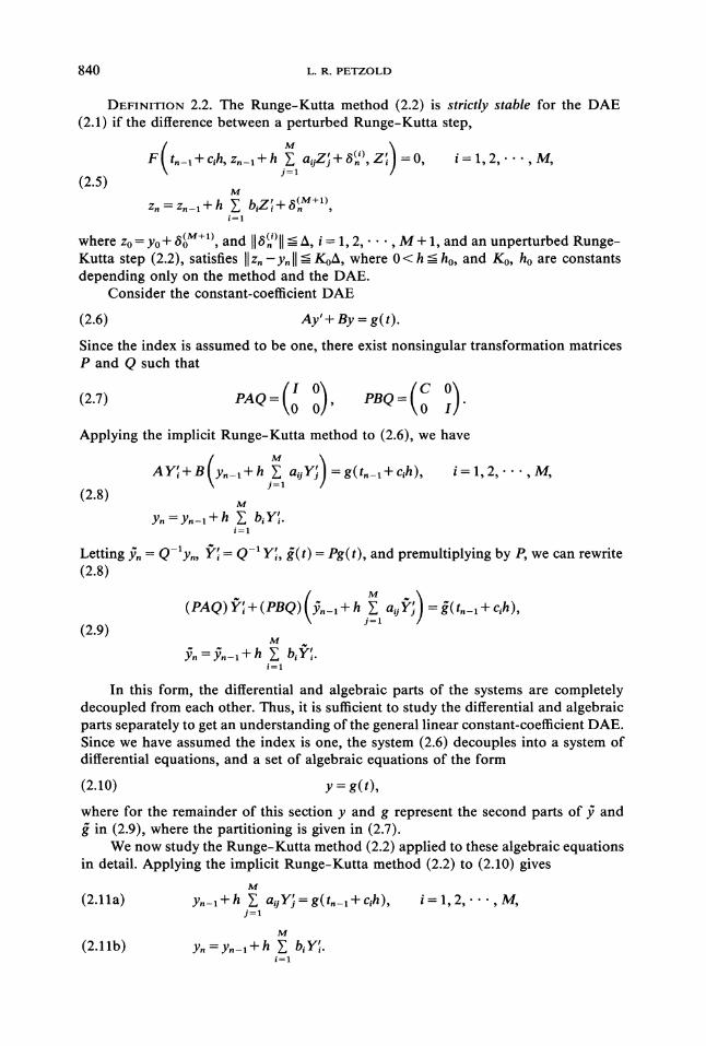
DEFINITION 2.2. The Runge-Kutta method (2.2) is strictly stable for the DAE(2.1) if the difference between a perturbed Runge-Kutta step,

F t_+qh, z_+h Y aoZj+,Z =0, i=l,2,...,M,j=l

(.51R(M+I)z,=z,_+h bZ+,,

i=1

where zo=Yo+ 6+), and 6), i= 1, 2,..., M+ 1, and an unpeurbed Runge-Kutta step (2.2), satisfies llz, -y, Ko, where 0< h ho, and Ko, ho are constantsdepending only on the method and the DAE.

Consider the constant-coefficient DAE

(2.6) Ay’ + By g( t).

Since the index is assumed to be one, there exist nonsingular transformation matricesP and Q such that

(2.7) PAQ=( 001 PBQ=(C )0

Applying the implicit Runge-Kutta method to (2.6), we have

AYI+B y_+h 2 aoY =g(t_+c,h), i=l,2,...,M,

(2.8/y, y,_ + h bY.

i=1

Letting f, Q-y,, Q- Y, (t) Pg(t), and premultiplying by P, we can rewrite(.81

(PAQ)Y+(PBQ) ,_,+h a, =(t,_l+C,h),(2.9)

M. ._+h E b,"g,.i=1

In this form, the differential and algebraic pas of the systems are completelydecoupled from each other. Thus, it is sucient to study the differential and algebraicpas separately to get an understanding of the general linear constant-coecient DAE.Since we have assumed the index is one, the system (2.6) decouples into a system ofdifferential equations, and a set of algebraic equations of the form

(2.10) y g(t),

where for the remainder of this section y and g represent the second pas of fi andin (2.9), where the paitioning is given in (2.7).We now study the Runge-Kutta method (2.2) applied to these algebraic equations

in detail. Applying the implicit Runge-Kutta method (2.2) to (2.10) givesM

(2.11a) Y,-I + h aoYj= g(t,-1 + c,h), i= 1, 2,..., M,j=l

M

(2.11b) Y, Y,-i + h b,Y.i=1


From (2.11) it is easy to see why we should assume the matrix M (aij) is nonsingular,for then Y’= (Y,. , Y)7" is determined uniquely by (2.11a).

To find the local error, let Y.-1 g(t._). Solving for Y’ in (2.11a), we have

(2.12a) Y’= M-G,where

/ (g(t,,-1 + Clh)-g(t,-l))/h I(2.12b) G={(g(t"-’+c2h!-g(t"-l))/h}.

\g._, + hi g_,))/h/Then from (2.11b), we have

(2.13) y. g(t._)+ hbTM-G,where b (bl, b2,’’’, b) Thus, the local error is given by

(2.14) d, g(t,_l) + hbr-iG g( t,).

Expanding the terms in (2.14) in a Taylor series around t,_l, we have

( h2 h3 h4gid.=- hg’+Tg"+g’"+ +...

.15 / ,_ch ,,_chcng .gg .

I ,_ch ,,_ch

I 2 h2

ng2g

6g

Equating like powers of h, d, O(h+) i br-c 1, j 1,. ., k where c(c, , c)Drro 2.3. The algebraic order of an implicit Runge-Kutta method (2.12)

is equal to k if d,= O(h+) for all equations (2.10) with g(t) suciently smooth.Then we have just shown,TOM 2.1. e algebraic order of an implicit Runge-Kutta method (2.2) is

equal to k iff the method coecients satisfy

(.) -,c= , j ,where

We now turn to the question of stability for linear constant-coefficient systems.Solving (2.10) by the perturbed Runge-Kutta method (2.5), we have

(2.17)

M

z._, + h E aoZj + 8)= g(t.-, + c,h ),j=l

M

z,, z,,_ + h biZ +i=1

i=1,2,...,M,

842 L.R. PETZOLD

Subtracting (2.17) from the corresponding expressions for the unperturbed solution(2.11), and letting e, y, z,, E’ Yi- Zi, we obtain

(2.18)

Rewriting,

M

e,-l + h Y aijEj- 8 0, 1, 2,..., M,j=l

M

e. en-l + h Y bE’ 8(M+I)i=l

(2.19) e, en-1 "k- b Ts-l(8n ete,_) 8+1),where eM (1, 1, , 1) T and 8, (8, 8,... ,8,t) 7-. Collecting terms,

(2.20) e, (1 b rM-1e)e,,-1 + (b’M-18, 6<4+1)).Thus we have shown,

THEOREM 2.2. An implicit Runge-Kutta method (2.2) is strictly stable for linearconstant-coefficient index one DAEs iff the method coefficients satisfy

(2.21) I1 b ’M-’eMI < 1.

We note that the inequality in (2.21) must be a strict inequality; for an examplesee M[irz [6].

Since DAEs can be regarded as "infinitely stiff" ODEs, it is natural to ask whatis the relationship between the above criterion for stability, and the stability criterionfor the same methods applied to the stiff model problem y’= Ay. From Hall and Watt[7], an implicit Runge-Kutta method (1.3) is stable for z= hA iff IR(z)l-< 1, where

(2.22)

It follows from (2.22) that

R(z) 1 + zbT(I-

lim R(z)=(2.23)Izl-

Thus, a method is stable for constant-coefficient index one DAEs if[

(2.24) r lim IR(z)I < 1.

Now that we have an understanding of the local truncation error and stabilityproperties of a method, we can estimate the size of the global error. Clearly, if r 0in (2.24) then the local error is equal to the global error, for the "algebraic part" ofthe system. For r < 1, we have from (2.20),

(2.25) Ile.II <-- rll e.-,ll + MA,where M is some positive constant, so that

(2.26) Ile.II-<- r"lleoll / 1 r ]MA.

Since r is independent of h and lim,_ ((1- r")/(1- r))= 1/(l-r) we have in thiscase that the order of the local error is the same as the order of the global error, forthe "algebraic part" of the system. Combining these results, we have

DEFINITXON 2.4. The constant -coefficient order ofan implicit Runge-Kutta method(2.2) is equal to kc if the method converges with global error O(h kc) for all linearconstant-coefficient index one systems (2.6) with g(t) sufficiently smooth.


THEOREM 2.3. The constant-coefficient order kc of the global error of an implicitRunge-Kutta method which satisfies

(1) the matrix sg of method coefficients is nonsingular,(2) the method coefficients satisfy the stability condition (2.21),

is given by

(2.27) kc- min (ka + 1, kd),

where kd is the order of the method for purely differential (nonstiff) systems, and k,, isthe algebraic order.

We see there is a reduction of order when k + 1 < kd. This order reduction effectactually does occur for some of the implicit Runge-Kutta methods in the stiff ODEliterature. Here we give examples of some implicit Runge-Kutta methods, along withtheir properties for constant-coefficient index one DAE systems.

METHOD 1 (Hall and Watt [7]). Semi-explicit third order Runge-Kutta.

3+x/ 3+x/0

6 6

3-x/ x/r 3+x/6 3 6

1 1

2 2

l+x/2+v/’

ka=3,

METHOD 2 (Burrage [8]). Singly implicit first order Runge-Kutta with errorestimate.

1 1

1

Error-estimating method,

1110 -1 1

2 2

844 L.R. PETZOLD

METHOD 3 (Burrage [8]). Singly implicit second order Runge-Kutta with errorestimate.

A (2 x/) A (4 ,f)/4 A (4- 3x/)/4A (2+x/) A (4+ 3x/)/4 A(4+,)/4

(4A(1 +v)-f)/(8A) (4A(1-x/)+f)/(8A)

A (2 + x/)/2,

a (4- 3/)/4 0

a(4+x/)/4 0

(a2(1 lx/- 8) a

bl b2 b3

b (6A2(2 + x/) 3A (3 +v) + 1)/(12A (A (3x/ 2) x/)),

b2 (6A 2(x/ 2) + 3A (3 -) 1)/(12A (A(3+ 2) -)),

b3 (6AE-6A + 1)/3(7A2- 6A + 1),

r .276,

k=3,

3. Nonlinear index one systems. In this section we study nonlinear index onesystems of the form (1.1). The Runge-Kutta methods are, in general, even less accuratefor nonlinear systems than for linear constant-coecient systems. The additional lossof accuracy comes about because of mixing which can occur between the differentialand algebraic pas ofthe solution. We give a set of order conditions which are sucientto ensure that a method is accurate to a given order for these systems.

To state our results, we need some notation. First, we must define the internallocal truncation errors, which are defined similarly in [5]

DEFINITION 3.1. The ith internal local truncation error " at t, of an M-stageimplicit Runge-Kutta method (1.5) is given by

M

" y(t._) + h aoy’( t._ + ch) y( t._ + c,h), , M,(3.1)

M

+=y(t,_l)+h b’(t,_l+C,h)-y(t,).i=1

r---0,

Error-estimating method,

A (2-x/) A (4-x/)/4A(2+v/) A (4+ 3x/)/41-A (-A2(1 lx/ + 8)

+4A (1 + 2x/) -v)/(SA + 4A (1 2v) +x/)/(8A


DEFINITION 3.2. The internal order kl of an M-stage implicit Runge-Kuttamethod (1.5) is given by

k1 min (k,..., k., kM+l)

where

t$i= O(hk’+l), i=1,..., (M+I).

It is simple to find the internal order of an implicit Runge-Kutta method in termsof its coefficients by expanding (3.1) in Taylor series around t,_, as in [5], leading to

THEOREM 3.1. The internal order of an M-stage implicit Runge-Kutta method is

equal to kt iff the method coefficients satisfy

cX aoc;-=- i=1 M,j=l k’

X bjc;-1= k

for k= l, ki.Following [1], we will say that a nonlinear system (1.1) is uniform index one if

the index of the constant-coefficient problem

Ay’( t) + By( t) g( t)

where A =OF/Oy’, B =OF/Oy is one in a neighborhood of the solution y(t), and if thematrices P, Q which transform (A, B) to the canonical form (1.8) satisfy:

(1) Q(t, y(t)) and Q-l(t, y(t)) exist and are bounded for all (t, y(t)) solving (1.1),(2) Q-l(t, ty(tl))Q(t2, y(t2)) I+O(t2-tl),(3) C( tl, y(t)) C( t2, y(t2)) + O(t2- tl).

These conditions are satisfied if in a neighborhood of the solution A and B aresufficiently smooth, the index is one, and the rank of A is constant.

Suppose the dimension of the "differential part" of the system is nl and thedimension of the "algebraic part" is n2. Then we can state the following result.

THEOREM 3.2. Suppose(1) System (1.1) is uniform index one.(2) F is linear in y’.(3) The Runge-Kutta method (1.5) satisfies the strict stability condition (2.21) with

0-<r<l.(4) The initial conditions satisfy Ilyo-y(to)ll- where k min (ka, kt + 1).(5) Ifk 1, then r O.

Then the global error of the Runge-Kutta method (1.5) is O(h).Proof. Consider the Runge-Kutta method (1.5). The numerical solution satisfies

(3.2a) F t,_1-4- c,h, y,,_ + h ao Yj, Y 0, 1, 2,. ., M,j=l

M

(3.2b) y,, y,-1 + h X b,Y.i=1

The true solution satisfies

( M )(3.3a)F t,_, + c,h, y( t,_,) + h E aoy’( t,-, + cjh ,, y’( t,_, + c,h O,

j=l

i=1,2,." .,M,

846 L.R. PETZOLD

M

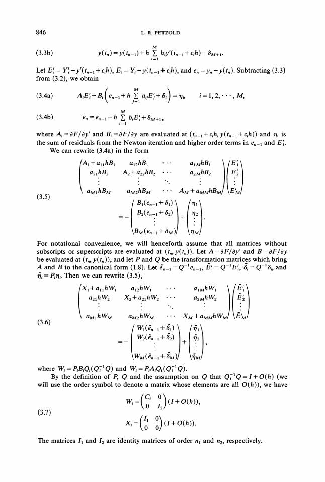
(3.3b) y( t,) y( t,_l) + h ,i=1

Let E= Y-y’(t,_ 4-cih), Ei Y-y(t,_l 4- ch), and e, y,- y(t,). Subtracting (3.3)from (3.2), we obtain

( M )(3.4a) A,E + B, e._l + h , aoE + 8, rl,, i= 1, 2,. ., M,j=l

M

(3.4b) e. e._l + h biE + 8M+I,i=1

where Ai=OF/Oy and B=F/Oy are evaluated at (t._ +cih, y(t._l +cih)) and rh isthe sum of residuals from the Newton iteration and higher order terms in e._ and E.

We can rewrite (3.4a) in the form

A + alhB

a21.hB2aMlhBM

(3.5)

a2hB aMhB1

A24-a.22hB2. "’’.. a2M.hBg_J;}aM2hBM AM 4- aMMhBM/ M/

B(e._ + 8)

B(e_..+8) + rl!\BM(e- +MFor notational convenience, we will henceforth assume that all matrices withoutsubscripts or superscripts are evaluated at (t., y(t.)). Let A =OF/Oy’ and B =OF/Oybe evaluated at (t., y(t.)), and let P and Q be the transformation matrices which bringA and B to the canonical form (1.8). Let .-1 Q-le.-, .’=i Q-1E’i, = Q-8i, and

r P:7. Then we can rewrite (3.5),

X 4- allhW al2hW1 alMhW \ /.

\ aMIIWM XM + aMMhWM/ \M]aM2hWM(3.6)

[ w,(._, + g,). ,/ w2(n-I 4- 82)

4- 2

\w(._, + .)

where W PBiQ(QT, Q) and W PAiQ(QT, Q).By the definition of P, Q and the assumption on Q that QC,Q I+ O(h) (we

will use the order symbol to denote a matrix whose elements are all O(h)), we have

W=(C’ O)(I+O(h))0 I2(3.7)

X, ( O0)(I+O(h)).The matrices I and I2 are identity matrices of order n and n2, respectively.


Partition/f (/(1),/(2)) r, where/(’) has dimension n and/(2) has dimension

n2. By partitioning 8i, n-i and in the same way, using (3.7) and rearranging thevariables and equations in (3.6), we can write

h2T2 (E. t(1) ( S1hT4 ] t(2)/=- hS3

(3.8) h2T3where

for i= 1, 2, and

T1 T + O(h),

T4= 4+ O(h),

S1 1 -t- O(h),

$4 I + O(h)

where l I + h/(R) C, 4 sg(R)/, S1 I(R) C, and %, T3, S, $3 are matrices whoseelements are O(1).

Let T, denote the left-hand matrix in (3.8). T, can be written as

(3.9) T,=hi hT3 4+ O(h)

T4 is inveRible because the matrix of coecients of the Runge-Kutta method isinveRible. By inveing the right-hand side of (3.9) the inverse of T, is given by

(310) T,=(’+O(h) O(h))O(h) 2/h + 0(1)

Using (3.10) to solve (3.8) for (’(, ’(:>) we have

,(1) TI

2+g:] +r ]"

Multiplying (3.4b) by Q-, which we now denote by Q to show its dependenceupon (t,, y(t,)) we obtain

M

i=l

Inseing (3.11) into (3.12), we have

(3.13) Oe.=S.O’e._-hU.g("+g+hr

848 L.R. PETZOLD

where

S. (i_ h (b- ll+ O(h)o(1) b2T1-1/h q" O(1)

0(1)O(h) )hr-I/h+O(1)2 .*4 I

Z1 IM () I1,

Z: e (R) I:,

b_=bV(R)I,,

b_= bV(R)I:,

0 b

where eM (1, 1,..., 1)r. By the definition of :4, we have

2-*4 Z2=(1-r)I2,

where r is defined in (2.24), and 0_-< r < 1 by the assumption that the method is stablefor constant-coefficient systems. Thus, S, has the form

(3.14) S,=K+O(h),

where

0 rISolving for en in (3.13), we obtain

e, Q._sS._sQ;lseo+ Q,_ss,_sQ-lj=l i=1 \j=O

(3.15)(hQ.,_,U,,_,g’-’) + Q._,)+ hQ._,B_ T._,-I -(n-i)) [

Now,

I-I Q,,-sS,,-s -s Q,, 1-I S,, -sQ-lsQ -s=o j=o

Q,,(K’* + O(h))Q-[

and

i--1

1-I Q,,-IS,-IQ-ll Q,(K’ + O(h))Q-l,+l.j=O


We can rewrite (3.15),

(3.16)Q-l e,, K + O(h )(Ql eo)

+ E (K’+ O(h))(hU,,_,g("-’)+ g_l + h_BTI,("-’)).i=1

Thus we find

(3.17)

n--1

.,=(K"+O(h)).o+ E (K’+O(h))hU,-,g(’-’)i=1

n--1 n--1

+ (K’+O(h))-+)l+ (K+O(h))h_BT-_,(-i).i=1 i=1

Let

u o b_;/hRewriting (3.17) and noting that I1,11- O(h’/), we have

e =(K + O(h))o+ K’(hO_g(-’+ g;)=1

(3.al+ (K’+ O(h))(hB_ T,_-I (n--i)) + o(hk’+l).

i=1

Observe that

(3.19) hlJn_ig(n-i)+g(-+i)=(O(hkd+l), O(hk+l)) r.We can see this by noting that the local error for the constant-coefficient problemA,z’(t) + Bnz(t) g(t) is given by

where ’ Qi, and we know from 2 that this local error is O(hk’/) in the differentialpart and O(hka+l) in the algebraic part. Although the solution to our problem and thesolution to the constant-coefficient problem are different, the cancellation of variousderivatives of the solution in the local error does not in general depend on the solution.Also note that because ’ O(h k, +1), h 0,_,g"-’) +g? O(hk,+1), O(hk,+l)) E Thusk >- kr. and ka>-k.

Suppose that II,’)ll _-< A,, o’)ll o(,), i= 1, 2. Expanding the terms in (3.18) andr O(1) and making use of (3.19), we find thatnoting that Y,=

.(,,’= 0(,)+ 0(h2)+ o(hka)+ o(hk’+’)+ O(A,)+ O(A2)(3.20)

)= O(h,)+ O(r:2) + O(h:2) + O(hk’+l)+ O(hA,) + O(A2).

For linear systems, A A2=0 and we can conclude that Ile.II- O(h), wherekG min (kd, kt + 1). For nonlinear systems, we sketch the proof. The higher orderterm is composed of terms of the form

..21e,,- +h a.iE+8, en-l.+h ., a.iEj+8,oy\ j=l j=l

(3.21)en_l+h aijE+i E’i.

Oy Oy =

850 L.R. PETZOLD

Thus we find that Ilfill is proportional to (ll - ll + hk)2/h. Substituting this relationfor r into (3.18), we obtain a nonlinear recurrence for ,. The solutions to this recurrencecan then be shown by induction to be of O(hk). We make use of assumption (5) ofthe theorem to bound the solutions to the recurrence.

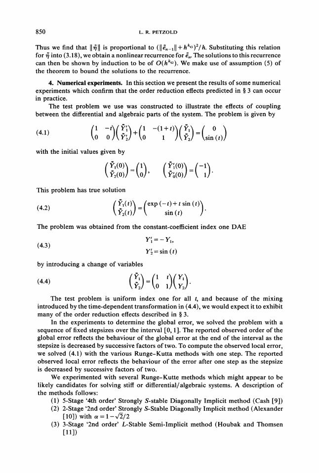
4. Numerical experiments. In this section we present the results of some numericalexperiments which confirm that the order reduction effects predicted in 3 can occurin practice.

The test problem we uso was constructed to illustrate the effects of couplingbetween the differential and algebraic parts of the system. The problem is given by

(4.1) (10 t)(+(10Y;]-(1+ 0

1 t))(yY.’)=(sin (t))with the initial values given by

,(o)

This problem has true solution

(4.2) I(t) sin(t)

The problem was obtained from the constant-coefficient index one DAE

(4.3)Y Y1,

Y sin (t)

by introducing a change of variables

1 Y(4.4) (12)--(0 )(Y2)The test problem is uniform index one for all t, and because of the mixing

introduced by the time-dependent transformation in (4.4), we would expect it to exhibitmany of the order reduction effects described in 3.

In the experiments to determine the global error, we solved the problem with asequence of fixed stepsizes over the interval [0, 1]. The reported observed order of theglobal error reflects the behaviour of the global error at the end of the interval as thestepsize is decreased by successive factors of two. To compute the observed local error,we solved (4.1) with the various Runge-Kutta methods with one step. The reportedobserved local error reflects the behaviour of the error after one step as the stepsizeis decreased by successive factors of two.

We experimented with several Runge-Kutte methods which might appear to belikely candidates for solving stitI or differential/algebraic systems. A description ofthe methods follows:

(1) 5-Stage ’4th order’ Strongly S-stable Diagonally Implicit method (Cash [9])(2) 2-Stage ’2nd order’ Strongly S-Stable Diagonally Implicit method (Alexander

[10]) with t 1-x//2(3) 3-Stage ’2nd order’ L-Stable Semi-Implicit method (Houbak and Thomsen

[11])


(4) 7-Stage ’3rd order’ Extrapolation method based on fully implicit backwardEuler and polynomial extrapolation, written as a semi-implicit Runge-Kuttamethod

(5) 3-Stage ’4th order’ Lobatto IIIc method (Chipman [12])(6) 2-Stage ’2nd order’ Singly-Implicit method (Burrage [8], described in 2)Table 4.1 gives the results of the experiments. In Table 4.1, kg is the order of the

observed global error and k6 is the lower bound which is predicted by the theory,based on ka and k.

Method

TABLE 4.1Numerical results.

kd ka kx+l k kg

4 oo 2 2 22 oo 2 2 22 2 2 23 oo 2 2 34 oo 3 3 42 o 2 2 2

Based on the results in Table 4.1, we can make a few observations. It is reassuringthat in no case was the lower bound for the order predicted by the theory higher thanthe order which was actually observed, and in many cases these two orders coincided.The observed orders for the extrapolation method and for the Lobatto IIIc formulawere higher than would be expected based on the theory. We do not know whetherall of the different order extrapolation methods based on backward Euler would havethis property, or even whether there might exist problems for which the observed orderis given by the lower bound.

Since k for a semi-implicit Runge-Kutta method is limited to one (because thefirst stage is necessarily a backward Euler step), we would expect the order of theglobal errors for these methods to be limited to two. This appears to be the case, withthe exception again being the extrapolation method, which can be written as a semi-implicit Runge-Kutta method. Orders higher than two appear to be easily achievedby going to a fully implicit formula such as the Lobatto IIIc method where the stageorders are higher. At least, in this case higher orders are predicted by the results in

3. We have yet to achieve a complete understanding of the order reductionphenomenon, as evidenced by the better than predicted behaviour of the extrapolationmethod reported in Table 4.1; however it is clear that many of the order reductioneffects predicted in the earlier sections actually do occur.

The orders that we predict and observe for the DAE systems tend to be somewhathigher than those predicted by Prothero and Robinson [4] and Frank, Schneid, andUeberhuber [5] for related classes of stiff systems. For example, the theory of Frank,Schneid, and Ueberhuber [5] predicts an order of one for the global error of allsemi-implicit Runge-Kutta methods for stiff systems, while we predict and observe anorder of two for those methods applied to index one DAEs. Neither set of results iswrong. The differences are due mainly to considering different classes of problems.For example, Prothero and Robinson [4] consider the model problem

(4.5) y’= a (y g(t)) + g’(t)

852 L.R. PETZOLD

for Re (-h) o and say that a method has order (p, q) if the error behaves as h’+h q

as Re (-hh) and h0.For methods where q =-1, the error behaves as hp+, but in addition it tends to

zero for any h as Re (-h). In [4], [5] these methods with q -1 are said to haveorder p, whereas for DAEs the order is infinite because these methods are exact forthe algebraic equation

(4.6) y=g(t)

which is the limit of (4.5) as Re (-h). By looking at DAEs, we see everything inthe limit as IAI- o. On the other hand, for stiff equations where 1’1 is very large, itmay be that the errors are already so small that the behaviour as h is reduced is notimportant. There is no question, however, that even after neglecting order reductioneffects which disappear as 1[-, order reduction can occur.

Acknowledgments. The author is grateful to G. Dahlquist and L. F. Shampine formaking her aware ofthe work of Frank, Schneid and Ueberhuber, and to S. L. Campbellfor his helpful comments.

REFERENCES

C. W. GEAR AND L. R. PETZOLD, ODE methods for the solution of differential/algebraic systems, thisJournal, 21 (1984), pp. 716-728.

[2] P. LtTSTEDT AND L. R. PETZOLD, Numerical solution ofnonlinear equations with algebraic constraintsI: convergence results for backward differentiation formulas, Math. Comp., to appear.

[3] R. MRz, Multistep methods for initial value problems in implicit differential equations,Humboldt-Universit/it zu Berlin, Preprint No. 22, 1981.

[4] A. PROTHERO AND A. ROBINSON, On the stability and accuracy of one-step methods for solving stiffsystems of ordinary differential equations, Math. Comp., 28 (1974), pp. 145-162.

[5] R. FRANK, J. SCHNEID AND C. W. UEBERHUBER, Order results for implicit Runge-Kutta methodsapplied to stiff systems, this Journal, 22 (1985), pp. 515-534.

[6] R. MXRZ, On difference and shooting methods for boundary value problems in differential/algebraicequations, Humboldt-Universitit zu Berlin, Preprint No. 24, 1982.

[7] G. HALL AND J. M. WATT, Modern Numerical Methods for Ordinary Differential Equations, OxfordUniv. Press, Oxford, 1976.

[8] K. BURRAGE, A special family of Runge-Kutta methods for solving stiff differential equations, BIT, 18(1978), pp. 22-41.

[9] J. R. CASH, Diagonally implicit Runge-Kutta formulae with error estimates, J. Inst. Math. Appl., 24(1979), pp. 293-301.

[10] R. ALEXANDER, Diagonally implicit Runge-Kutta methodsfor stiff ODEs, this Journal, 14 (1977), pp.1006-1022.

11] N. HOUBAK AND P. G. THOMSEN, A FORTRAN subroutinefor the solution ofstiff ODEs with sparseJacobians, Technical University of Denmark, ISSN 0105-4988, 1979.

[12] F. H. CHIPMAN, A.stable Runge-Kutta processes, BIT, 11 (1971), pp. 384-388.

results applied differential/algebraic systems*

Documents