restoring whitebark pine in the sierra nevada: prescribed … · restoring whitebark pine in the...

Kelsey P. Lyberger Restoring Whitebark Pine in the Sierra Nevada Spring 2014

1

Restoring Whitebark Pine in the Sierra Nevada: Prescribed Burning Suitability Analysis

Kelsey P. Lyberger

ABSTRACT

Whitebark pine is a keystone species of the upper subalpine ecosystem of western North America.

Unfortunately, it is in danger of extinction in as few as two generations. In the recent past, humans

have played a major role in the decline of whitebark pine, not only by introducing an invasive

pathogen and expanding the range of deadly bark beetles through climate change, but also by

preventing periodic fires, which increases competition with other species of trees. Although

vegetation management and prescribed burning restoration efforts in whitebark pine’s devastated

northern ranges have had limited success, the less infected forests of the Sierra Nevada Mountain

Range provide an excellent opportunity to implement prescribed burning. In this study, a suitability

analysis was used to prioritize stands for prescribed burning that vary in terms of ecological

parameters, such as the presence of the mutualistic bird, Clark’s nutcracker, and environmental

parameters, which affect the practicality of setting a controlled fire. The addition of these weighted

opportunities and constraints resulted in a map that highlights the high elevation, mid and central

areas of the Sierra Nevadas as good regions for restoration. 1.6% of the land is suitable, covering

over 87 thousand acres, according to the final suitability map. Given the availability of suitable

restoration sites and their locations, federal land managers can begin the process of planning

prescribed burns to protect this endangered species.

KEYWORDS

Subalpine community, ArcGIS, site selection, Clark’s nutcracker, fire


2

INTRODUCTION

Interspecies interactions play a critical role in shaping forest ecosystems (Bertness and

Callaway 1994). The dynamics between species are often disrupted when invasive species are

introduced. Invasive pathogens and insects, such as the chestnut blight fungus, the Dutch elm

disease fungus (Castello et al. 1995), and the elm ash borer (Poland and McCullough 2006) all

influence forest ecosystems via tree mortality. These and other pathogenic invasive species have

created the need for forest protection and restoration across the United States. Entire landscapes

are changing because once dominant trees are dying off. High tree mortality after infestation leads

to accelerated succession, increased fuel loading, increased stream flow, and altered chemical

cycling on large scales (Raffa et al. 2008).This problem is exemplified by the keystone species

whitebark pine, Pinus albicaulis, which is declining throughout its range in the subalpine

communities of western North America, predominantly due to the introduction of white pine

blister rust (WPBR) and other anthropogenic influences.

Over the last few hundred years, humans have contributed to the decline of whitebark pine

by promoting threats including disease, fire suppression, and climate change. Humans introduced

the invasive tree disease species WPBR, a native of Eurasia, to British Columbia in 1910 (Hoff

and Hagle 1990). Since then, WPBR has been slowly killing five needle white pines, by infecting

their cone bearing branches and then girdling their trunks with blisters, as it spreads south over

whitebark pine’s entire range (Maloney 2011, Tomback et al. 2001). By implementing a policy of

fire suppression, which alters stand dynamics, humans have also influenced the health of this forest

ecosystem (Arno 1996). Instead of being periodically killed by burns, the shade tolerant species

mountain hemlock (Arno and Hoff 1989) and lodgepole pine (Peterson et al. 1990), compete with

and replace whitebark pine (Tomback et al. 2001). The added stress from competition and the

increased age of whitebark pines have also made them more susceptible to infestation and death

by the mountain pine beetle (MPB) (Cole and Amman 1969, Peterman 1978). MPB is of

heightened concern because climate change has allowed it to expand its range northward and to

higher elevations (Carroll et al. 2003). These pressures similarly threaten other aspects of the

pine’s life-cycle strategy, including reproduction.

The success of the next generation of whitebark pine is affected by a complex series of

ecological interactions including mutualism and predation. Whitebark pine cones are indehiscent,


3

meaning that they cannot distribute their own seeds, and therefore obligately rely on Clark’s

nutcracker, Nucifraga columbiana (Tomback 1982). This mutualism is critical to whitebark pine

population regeneration and its success is multifactorial. First, there must be a large enough seed

crop available to granivores, the animals that rely on seeds as a food source. In this case, Clark’s

nutcrackers are able to bury many more times the number of seeds they can retrieve and eat, leaving

the rest to germinate (Tomback 1982). Other granivores include rodents, such as the red squirrel

and Douglas squirrel, which forage on whitebark pine cones and predate the seeds. Large

population sizes and high mobility of these rodents have a negative effect on seed dispersal

probabilities (Siepielski and Benkman 2007). Unfortunately, whitebark pines are not producing

enough seeds to exceed the demands of granivores and this natural system is no longer working.

In as little as 120 years, whitebark pine is in danger of becoming extinct (USFWS 2014). Thus,

restoration efforts are needed to help this endangered species.

Currently, management and prescribed burning restoration efforts are centered in

whitebark pine’s northern ranges, the Rocky Mountains and Cascade Range, where mortality is

highest (Keane and Parsons 2010a, Warring and Six 2005, Burns et al. 2008). The prevalence of

WPBR increases with latitude (Maloney 2011) and the worst MPB outbreaks occurred in Idaho

and Montana (Bartos and Gibson 1990). This region is where restoration techniques have been

tested. The preferred restoration technique involves prescribed burning that mimics historical fire

regimes to kill the understory and promote areas where Clark’s nutcracker caches seeds (Keane

2001). Prescribed burning is a good strategy because whitebark pine is better at surviving and

regenerating after fire than associated species because of its thicker bark, thinner crowns and

deeper roots (Arno and Hoff 1990). Unfortunately, prescribed burning has failed in areas

surrounded by high mortality and low seed producing stands, due to the birds reclaiming all cached

seeds within the newly burned, open areas (Keane and Parsons 2010a). In cases where the seed

sources are too low, seedlings must be hand planted in treated areas, which is much more expensive

and labor intensive than burning techniques (Keane and Parsons 2010b). The Sierra Nevada

Mountain Range, located much further south than current restoration areas, provides an excellent

opportunity to implement prescribed burning because disease rates are still low. However, areas

where restoration efforts should be directed have not yet been identified.

The objectives of study were to determine where prescribed burning is likely to be

successful in managing populations of whitebark pine in its Sierra Nevada distribution. I located


4

sites where ecological parameters, such as the presence of Clark’s nutcracker, serve as

opportunities and constraints to the success of the next generation of whitebark pine. I also

included environmental parameters like slope, temperature, and wind speed, which all affect the

practicality of safely and successfully burning a site. I used suitability analysis to prioritize stands

that vary spatially in terms of twelve key ecological and environmental considerations for setting

prescribed burns. Ultimately, this produced a series of maps that highlight areas that are good

candidates for restoration as well as unsuitable areas that should be avoided.

METHODS

Study system

To study whitebark pine restoration using prescribed burning, I chose to focus on the

subalpine region of the Sierra Nevada Mountain Range. This range is home to the southernmost

population of whitebark pine. Whitebark pine’s complete distribution includes regions in western

Canada, as well as regions extending through the Sierra Nevada Mountains, the Cascade Range,

and throughout the northern half of the Rocky Mountains. It occurs, although not continuously,

between 107° and 128°W and between 37° and 55°N (McCaughey and Schmidt 1990). The Sierra

Nevada is composed of nine national forests, three national parks and two national monuments. It

covers almost 100,000 km² and extends latitudinally from 35°06′08″N to 40°21′32″N and

longitudinally from 118°16′58″W to 120°52′3″W. Although the Sierra Nevada Mountain Range

covers a large area, whitebark pines only grow in the subalpine zone, in elevations from 3000 to

4000m (Peterson et al. 1990). The area I analyzed is restricted by both the boundary created by the

seven national forests and two national parks that whitebark pine exists within and the boundary

created by the farthest a Clark’s nutcracker has been known to carry whitebark pine seeds, which

is 22 miles from the source (Lorenz 2011).


5

Data collection

To determine what parameters would affect the restoration suitability of an area, I found

evidence through expert biologists’ input and published research findings. Limited by the data

readily available, I narrowed the countless variables down to twelve (Table 1).

Table 1. Description of parameters used for the suitability analysis.

Parameter Category Description and Reasoning Weight

Whitebark pine Ecological A nearby seed source is needed for

regeneration.

20

Lodgepole Pine Ecological This is a climax species that competes with

Whitebark pine for resources.

10

Mountain Hemlock Ecological This is a climax species that competes with

Whitebark pine for resources.

10

Clark’s Nutcracker Ecological A seed disperser is needed to open cones and

cache seeds.

15

Temperature Environmental Higher temperatures allow for high intensity

burns.

15

Wind Environmental Fires become unpredictable in no wind or

quickly spreading in high wind conditions.

10

Developed Land Environmental Fires must be as far away from buildings as

possible.

15

Barren Land Ecological Although these are open areas, seedlings will

not germinate on rock.

10

Slope Environmental Easier to control burns on moderate slopes

compared to flat or extremely steep slopes.

10

Aspect Environmental Dryer, south facing slopes burn better than

wetter north facing slopes.

10

Distance to Roads Environmental Roads allow access to a site and act as fire

breaks. Also reduces cost.

20

Fire Return Interval

Departure

Ecological Lack of recent burns, increases competition

and risk of disease outbreak.

15


6

To obtain spatial data on whitebark pine and Clark’s nutcracker to create species

distributions, I searched a number of online databases and publications. From “The distribution of

forest trees in California” (Griffin and Critchfield 1972), I hand-digitized the ranges of whitebark

pine, lodgepole pine, and mountain hemlock in ArcGIS 10.1 (ESRI 2011). To create the

distribution map of Clark’s nutcracker, I also downloaded species occurrence data from the Nature

Mapping Foundation’s California Gap Analysis Bird Maps (Davis et al. 1998).

In addition to these species distributions, this study required data on environmental

characteristics of the landscape. One set was climate data, in the form of mean temperature, which

was downloaded from the PRISM Climatic Group (Daly 2008). Wind data was found through the

National Renewable Energy Laboratory (http://www.nrel.gov/gis/wind.html). I also downloaded

land cover types, which are categorized based on their distinct spectral signatures, at the 3 arc

second resolution level from the USGS National Map Viewer (viewer.nationalmap.gov/).

Specifically, I added the building/urban cover and rock cover categories as layers in this study. I

also downloaded elevation data from the USGS National Map Viewer. Using the Digital Elevation

Model (DEM), I calculated slope and aspect. Spatial data on Californian infrastructure, such as

roads, was downloaded from TIGER/Line (US Census Bureau, census.gov/geo/www/tiger/).

Finally, fire return interval departure (FRID) was included to represent the ratio of the time elapsed

since the last burn and the time between burns given a pre-settlement fire regime. I obtained this

from the Forest Service’s GIS Clearinghouse (fs.fed.us/r5/rsl/clearinghouse/r5gis/frid/).

Suitability model

To produce a composite map highlighting high priority stands for restoration, I used a land-

use suitability mapping analysis in ArcGIS 10.1 (ESRI 2012). A suitability analysis is a method

of site selection analysis to identify the optimal site for a desired activity given the set of potential

sites (Malczewski 2004). After the initial data collection, each layer was stored into a single

geodatabase and added into ArcMap as either a raster—a set of uniform squares on a grid, where

areas are groups of adjacent cells with the same value—or a vector—a set of polygons, lines, and

points that are coordinate based. Many layers contained extraneous attributes, which were

removed. Layers that were undefined or used a different geographic coordinate system were

defined or transformed to NAD 1983.

http://www.fs.fed.us/r5/rsl/clearinghouse/r5gis/frid/


7

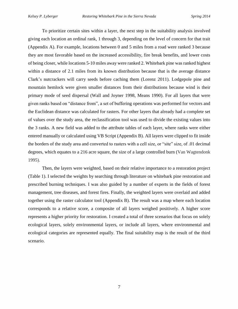
To prioritize certain sites within a layer, the next step in the suitability analysis involved

giving each location an ordinal rank, 1 through 3, depending on the level of concern for that trait

(Appendix A). For example, locations between 0 and 5 miles from a road were ranked 3 because

they are most favorable based on the increased accessibility, fire break benefits, and lower costs

of being closer, while locations 5-10 miles away were ranked 2. Whitebark pine was ranked highest

within a distance of 2.1 miles from its known distribution because that is the average distance

Clark’s nutcrackers will carry seeds before caching them (Lorenz 2011). Lodgepole pine and

mountain hemlock were given smaller distances from their distributions because wind is their

primary mode of seed dispersal (Wall and Joyner 1998, Means 1990). For all layers that were

given ranks based on “distance from”, a set of buffering operations was performed for vectors and

the Euclidean distance was calculated for rasters. For other layers that already had a complete set

of values over the study area, the reclassification tool was used to divide the existing values into

the 3 ranks. A new field was added to the attribute tables of each layer, where ranks were either

entered manually or calculated using VB Script (Appendix B). All layers were clipped to fit inside

the borders of the study area and converted to rasters with a cell size, or “site” size, of .01 decimal

degrees, which equates to a 216 acre square, the size of a large controlled burn (Van Wagtendonk

1995).

Then, the layers were weighted, based on their relative importance to a restoration project

(Table 1). I selected the weights by searching through literature on whitebark pine restoration and

prescribed burning techniques. I was also guided by a number of experts in the fields of forest

management, tree diseases, and forest fires. Finally, the weighted layers were overlaid and added

together using the raster calculator tool (Appendix B). The result was a map where each location

corresponds to a relative score, a composite of all layers weighed positively. A higher score

represents a higher priority for restoration. I created a total of three scenarios that focus on solely

ecological layers, solely environmental layers, or include all layers, where environmental and

ecological categories are represented equally. The final suitability map is the result of the third

scenario.


8

Data analysis

Although the results of this study are primarily meant to be disseminated visually, to better evaluate my research question, I also performed a hotspot analysis and analyzed the sensitivity of each layer. Within each of the three scenarios, this analysis looked at the range and spread of scores and the percentage and acreage

of sites considered suitable, moderately suitable, and unsuitable. General trends across the study area were described based on visual color patterns. The locations of the highest scored areas were identified using the select by attributes tool. Within these sites, the ranks of each layer was determined using the identify tool to isolate

which layers are constraining. To determine the prevalence of statistically significant clumped suitable locations, I used the hotspot analysis tool. The hotspot analysis tool identifies statistically significant spatial clusters of high and low scores, attributing a p-value for each site. The p-values indicate if the scores of the sites are

more clustered in the model than if the same set of scores were randomly distributed. I used α=.05 to classify low scoring clusters with a p-value below .05 as “cold spots” and high scoring clusters with a p-value above .95 as “hot spots”.

To determine the sensitivity of the model, I looked at all layers individually and in relation to each other. The mean rank of the layer hints at the amount it serves as an opportunity or constraint. Furthermore, I considered the distribution of a layer’s ranks across the study area and their relation to other layer’s ranks to

determine which are unlikely to have high ranks that overlap. For layers with suspected negative correlations, I ran the Band Collection Statistics tool. Layers that often act as the constraining parameter for suitable sites are especially important to the model.

RESULTS

Ecological map

The scores of the ecological map range from 80 to 240 (Figure 1a) and are distributed normally. These scores are classified as follows: 80-130 is unsuitable, 135-185 is moderately suitable, and 190-240 is suitable. 21% of the total study area is unsuitable, 69% is moderately suitable, and 10% is suitable (Figure 2). These

percentages equate to 1,174,176 acres of unsuitable area, 3,831,408 acres of moderately suitable area, and 543,672 acres of suitable area. Suitable areas are generally located at high elevations in the interior of the study area.

Four sites have a score of 240 because they have the highest rank for all six ecological layers. The satellite image of one of these sites shows that the land is covered in a dense coniferous forest. Fourteen other sites have a score of 230. The majority of these sites are only missing the highest rank for the barren land layer,

and a few are missing the highest rank for the FRID layer. One is missing mountain hemlock and another is missing lodgepole pine. The hotspot analysis results in many more contiguous cold spots than hot spots, which are isolated and scattered across the study area (Figure 2).


9

Figure 1.

Suitabiliy of areas for the Ecological Scenario. The warmer, redder colors represent a higher suitability and the colder, bluer colors represent a lower suitability. The legend shows a continuous spread of scores.

Score

Satellite image of

a top scoring site,

located at the

intersection of

Vleck Spur and

Red Peak Road in

El Dorado

National Forest.


10

Figure 2.

The first map (left) is the Ecological Scenario classified into the 3 equal range categories, and (right) is the result of the hotspot analysis classified based on p-value.

Environmental map

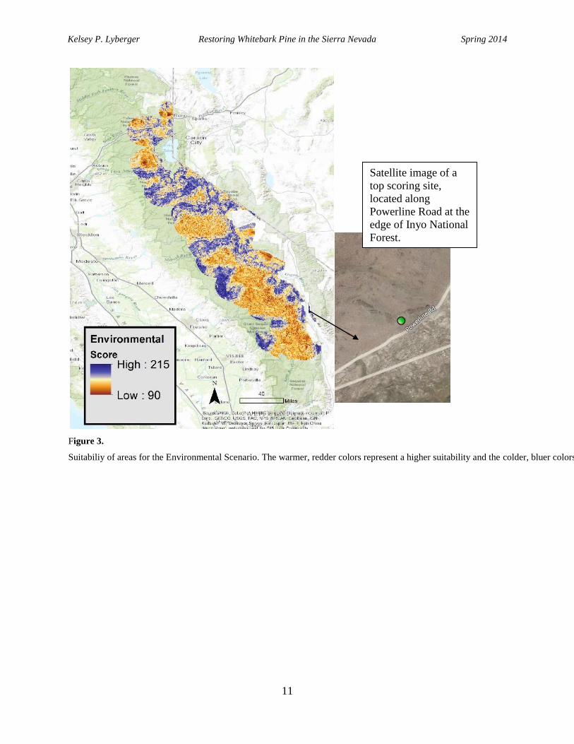
The Environmental Scenario had a possible range of 80 to 240, but actual scores ranged from 90 to 215 (Figure 3). The scores were classified the same as the ecological scenario. 19% of the study area is unsuitable, 76% is moderately suitable, and 5% is suitable (Figure 4). These percentages equate to 1,075,896 acres of

unsuitable area, 4,186,664 acres of moderately suitable area, and 269,784 acres of suitable area. Suitable areas are generally located around the edge of the study area often at low elevations. The exception to this trend is the northern central region of the study area. The unsuitable areas cover large regions in the high elevation,

mid to low latitude Sierra Nevadas.

None of the sites were ranked high for all six layers. Two sites scored 215, and were missing a combination of wind, temperature, aspect, and slope. The satellite image of one of these sites shows that although a burn at this site is most likely to be safe and successful, the land is does not have trees and therefore will serve

little purpose for land managers who have the objective of restoring whitebark pine. Eighteen other sites have a score of 210. The majority of these sites are missing the highest rank for temperature. The hotspot analysis results are similar to the Ecological Scenario in that cold spots cover a much larger area and hot spots are

smaller and more isolated from each other (Figure 4). However, both types of clusters are less contiguous, especially in the north, and the hot spots are more numerous.

Ecological Hotspot Analysis

Low Spot Hot Spot

Not Significant.

Ecological Suitability Classes

Unsuitable

Moderately Suit.

Suitable


11

Figure 3.

Suitabiliy of areas for the Environmental Scenario. The warmer, redder colors represent a higher suitability and the colder, bluer colors represent a lower suitability. The legend shows a continuous spread of scores.

Satellite image of a

top scoring site,

located along

Powerline Road at the

edge of Inyo National

Forest.


12

Figure 4.

The first map (left) is the Environmental Scenario classified into the 3 equal range categories, and (right) is the result of the hotspot analysis classified based on p-value.

Composite final map

The Final Scenario had a possible range of 160 to 480, but actual scores ranged from 210 to 425 (Figure 5). These scores are classified as follows: 160-265 is unsuitable, 270-375 is moderately suitable, and 375-480 is suitable. 8.6% of the study area is unsuitable, 89.8% is moderately suitable, and 1.6% is unsuitable (Figure

6). These percentages equate to 476,712 acres of unsuitable area, 4,977,936 acres of moderately suitable area, and 87,696 acres of suitable area. Suitable areas are generally located at high elevations in the northern central region of the study area.

The most suitable site received a score of 425 because it is not ranked highest in the temperature, FRID, and barren land layers. The satellite image of one of these sites shows that the land is a partially open and partially a subalpine coniferous forest. The image shows a landscape that looks intermediate between the top

sites in the Ecological and Environmental Scenarios. The one site that scored second highest at 420 and the nine sites that scored 410 are most often lacking the optimal temperatures and distance from barren land. They are secondarily lacking high ranks for wind and slope. Whitebark pine, Clark’s nutcracker, and distance from

developed land are positively attributed to all eleven high scoring sites. Compared to the other scenarios, the significant clusters are more isolated from each other (Figure 6). The distribution of hot spots and cold spots in the Final Scenario is similar to the Environmental Scenario, but the less contiguous clusters are in the south.

Environmental Hotspot Analysis

Low Spot

Hot Spot

Not Significant

Environmental Suitability Classes

Unsuitable Suitable

Moderately Suitable


13

Figure 5.

Suitabiliy of areas for the Final Scenario. The warmer, redder colors represent a higher suitability and the colder, bluer colors represent a lower suitability. The legend shows a continuous spread of scores.

Satellite image of the top

scoring site, located 1km

south of Cowcamp Creek,

near Sonora Junction, in

Toiyabe National Forest.


14

Figure 6.

The first map (left) is the Final Scenario classified into the 3 equal range categories, and (right) is the result of the hotspot analysis classified based on p-value.

Model Sensitivity

Each layer had a distinct distribution of high, medium, and low ranked sites (Appendix C). Layers with the highest mean rank were Clark’s nutcracker (µ=2.62) and developed land (µ=2.42). As expected, neither of these parameters constrains the top suitable sites in the three scenarios. Layers with the lowest mean rank

were mountain hemlock (µ=1.19) and wind (µ=1.24). Mountain hemlock has a relatively small range compared to other 2 trees, covering only 6% of the study area. The worst wind power classes, 1 and 7, cover 83% of the study area and the best wind power classes are concentrated on high mountain ridges.

Although the barren land layer has a mean of 1.99, it is a constraint for many of the top suitable sites in both the Environmental and Final Scenarios. The barren land layer is negatively correlated with the wind layer (-0.18), suggesting that these parameters often do not both rank highly. Similarly, temperature and wind are

negatively correlated (-0.21) and FRID and barren land are negatively correlated (-0.134). Another reason why temperature and barren land are repeatedly identified as the constraining layer is that they both have higher ranks at lower elevations, whereas many other layers, like the three tree species, wind, and FRID, have higher

ranks at higher elevations.

DISCUSSION

The lack of suitable locations to implement prescribed burning to restore whitebark pine is evident in the differently weighted scenarios and final suitability map. Suitability was not commonly attained because there are a number of layers that are especially constraining and because sites with suitable ecological layers

tended to also have fewer suitable environmental layers and vice versa. However, in the past, the entire Pacific Southwest Region of the Forest Service only burned 54,401 acres annually (Cleaves et al. 2000). The 1.6% of the study area that is classified as suitable surpasses this amount of land, covering 87,696 acres.

Final Map

Hotspot Analysis

Low Spot

Hot Spot

Not Significant

Final Map

Suitablility Classes

Unsuitable Suitable Moderately Suitable


15

The majority of the highly suitable locations in the final map are widespread in southeast El Dorado National Forest, on the border of Toiyabe and Stanislaus National Forest, and in the center of Yosemite National Park. This finding is not surprising given these areas are in the core of whitebark pine’s distribution. Given

the locations of suitable restoration sites, federal land managers can begin the process of planning prescribed burns to protect this endangered species.

Scenarios

The two categorical scenarios have different spatial trends, suggesting that areas with highly ranked ecological layers are associated with lowly ranked practical layers. The most suitable areas in the Ecological Scenario (Figure 1) are located in the high elevation, central Sierra Nevada Range, because this is where most

whitebark pine stands occur, along with the other sub-alpine species mountain hemlock and lodgepole pine. This highly suitable area is a subset of the region where Clark’s nutcracker prefers because it relies on cones as a food source (Tomback 1982). Finally, the high elevation areas are where the FRID is largest and stands have

reached late successional stages. There were four sites that rank highest for all layers, which I consider perfectly suitable. However, most sites are only suboptimal because they contain or are near, bare rock and therefore don’t permit germination (Arno and Hoff 1990). Choosing among these suboptimal sites will require planners

to make tradeoffs, for example, between sites located away from barren land and sites with a high FRID Index. Planners will be able to benefit from the clustering of high scoring sites. Because there are contiguous hot spots, prescribed burning plans can be formulated for a region encompassing multiple suitable sites. The formation

of hot spots and cold spots also proves that the scores are not distributed randomly, signifying the model’s success.

In contrast to the Ecological Scenario, the most suitable areas in the Environmental Scenario (Figure 2) are located along the edges of the study area, only coming in towards the center where roads cut across. Many locations do not meet the wind requirement and the temperature requirement because these factors vary

inversely (Lookingbill et al. 2003, Hadley and Smith 1986). There are no sites that rank highest for all six factors. Unlike the Ecological Scenario, the suitable regions in the Environmental Scenario are more isolated and spread latitudinally, longitudilly and across a larger elevation gradient. The greater number of hot spots in the

Environmental Scenario and the Final Scenario allows for selection in more regions, but their smaller size is less conducive to planning larger controlled burns.

Because the ecological and practical layers are not in agreement, it is especially necessary for land managers to consider if the relative importance of each category should be equal (Tomback et al. 2001). For example, meeting the “distance from barren land” restriction results in less optimal wind speeds. This will require

management to make decisions about tradeoffs between factors like convenience, likelihood of whitebark pine regeneration, and cost of burning. The most suitable areas found in the Ecological Scenario will have success establishing new stands and reducing the problem of disease, whereas the most suitable areas found in the

Environmental Scenario will be less costly, more efficient, safer, and easier to burn (Biswell 1989).

Final suitability of whitebark pine distribution

Highly suitable areas were located mainly in the northern central Sierra Nevadas (Figure 6). This makes sense given that in these areas, whitebark pine covers a greater extent, symbiotic species are present, fire is overdue, accessibility is less of a problem, and weather conditions are favorable. However, there was no one

location that fulfilled all of the requirements, which is consistent with the findings of similar studies performed in the Rocky Mountains (Keane and Arno 1996). For example, a study was done to analyze the suitability of five sites in the Smith Creek Watershed using a weighted matrix similar to mine, but with fewer parameters

(Tomback et al. 2001). In that study, even the stand that was found to be the top priority lacked two factors and received a score of 96 out of 108.

The suitable areas are located within El Dorado, Toiyabe, and Stanislaus National Forests and Yosemite National Park. It is likely that managers would approve of prescribed burning here (AEU Strategic Fire Plan). Considering the opportunities and constraints attributed to these areas, a project here will not be too costly.

Each site will need to be looked at individually because in some cases where the fire prerequisites like slope, wind speed and temperature are not met, other strategies such as using mechanical cutting treatments may be considered (Burns et al. 2008). An additional consideration that would increase the probability of a successful

next generation is to plant rust resistance seedlings after a burn clears and area. However, this technique is more costly and should be done where there is a danger that seedling recruitment will be low, such as in areas further from current whitebark pine stands (Samman et al. 2003, Whitebarkfound.org).

Model sensitivity

The layers that were the most important to the map were barren land and temperature, due to their lack of high ranks in top suitable locations, as well as wind and mountain hemlock, due to their lower mean ranks. Surprisingly, barren land and wind were not considered as important parameters in the literature (Tomback et

al. 2001, Biswell 1989). Fortunately, some of these constraints can be relaxed. For example, even if a site is not attributed to the optimal mean temperature range or mean wind speed range, it is likely that during certain days of the year, these requirements for setting a prescribed burn will be met. In a similar manner, sites that do

not include mountain hemlock should still be considered, because it is still necessary to open up late succession forests where lodgepole pine is competing with whitebark pine.


16

Slope and aspect had almost no influence on the model, given that they are evenly distributed across the landscape. These parameters may play a larger role in a smaller scale model, where sites within a single watershed are considered. Almost all areas meet the distance from developed land requirement because the range

of whitebark pine is primarily in wilderness lands (Taylor et al. 2014). Whitebark pine, lodgepole pine, and FRID also do not tend to bring down the suitability of top sites. The two species of trees occupy a lot of the same subalpine zone, which is also where there has been a lack of fire. Clark’s nutcracker was not important to the

model, given its widespread distribution. This finding does not match the literature, which puts a larger emphasis on prioritizing the presence of Clark’s nutcracker (Tomback 1982, Arno and Hoff 1989)

Unfortunately, I did not have access to a panel of land managers, who would directly influence the weight given to each layer by stating their preferences. Therefore, the weights are biased (Malczewski 2004). On the other hand, GIS is a strong tool and due to the success of this model, suitability analyses should be used to

investigate prescribed burning restoration sites over whitebark pine’s entire range in southern Canada, the Cascade Range, and the Rocky Mountains. In the more decimated populations, the success of this model is contingent on the inclusion of additional variables to account for rates of disease. This model could also be run for

similar species of concern, in which scientists have yet to identify of areas for restoration.

Limitations and future directions

Accuracy of some of the spatial data was limited to what I could freely access online or in print. There are multiple sources from which I could access the species distributions of the three tree species I mapped. I chose to hand digitize and georeference physical maps that were published over four decades ago. This method

introduced human error and ignored the changes in the distributions over time. To reduce these errors, the next step is to combine multiple sources such as the more recent survey data from the California Native Plant Society Vegetation Program and the Forest Inventory and Analysis (Taylor et al 2014, www.fia.fs.few.us). To

improve the accuracy of the FRID, fires that occurred after 2011 should be incorporated. For example, The Rim Fire in Yosemite National Park and Stanislaus National Forest burned over 257,000 acres, yet it was not included in the model despite its intensity and magnitude (Veraverbeke et al. 2013).

To fine tune the model beyond including more up to date and accurate sources of data, other variables that are important to whitebark pine restoration can be included as additional layers. Unfortunately, many of these have not been mapped in the Sierra Nevadas. Examples are the distribution, disease outbreak risk, and

infection rates of MPB and WPBR. On a much smaller scale, the percent canopy cover is an important variable that I had to dismiss (Keane et al. 2012). Even with the inclusion of all the variables that could be considered important, a suitability analysis is still just a model of reality. In forming the model, complex species

interactions, geography, and land characteristics must be oversimplified. To address this problem, the next step in the restoration process is to determine if the chosen highly suitable sites are realistically okay to burn by physically surveying the sites. Ground truthing these locations is necessary to verify that they have the

characteristics of a suitable site (Hyypa et al. 2000).

Broader Implications

The results of this study are meant to influence decisions of park managers in order to conserve whitebark pine using an approach that integrates both ecologically-based and practical-based requirements. The most suitable locations found by this model fulfill the requirements set by the Forest Service to undergo a prescribed

burn (AEU Strategic Fire Plan). Planning should begin soon, while prescribed burning is still a viable option for restoring whitebark pine. Because the suitable areas I identified contain high rankings of succession and fire return interval departure, the need for restoration is urgent and widespread (Keane 2001). The future of this

endangered species depends on actions taken now, in the Sierra Nevada Mountain Range.

ACKNOWLEDGEMENTS

I thank the ESPM 175 professors and GSI’s: Patina Mendez, Kurt Spreyer, Rachael Marzion and Ann Murray for their support and encouragement. I also thank Kelly Iknayak for her initial guidance on my project. Special thanks to the staff of the Geospatial Innovation Facility for providing access to ArcMap enabled

computers and for their help in office hours. Lastly, I couldn’t have gone through the many revisions to improve my project without the constructive criticism of my friends, family, and the 175 class workgroup.

REFERENCES

http://www.fia.fs.few.us/


17

Arno, S. 1996. The seminal role of fire in ecosystem management-impetus for this publication. Pages 3-5

in Hardy, Colin C.; Arno, Stephen F., editors. The use of fire in forest restoration. General

Technical Report INT-GTR-341. USDA [United Stated Department of Agriculture] Forest

Service, Intermountain Research Station. Ogden, UT, USA.

Arno, S., and R. Hoff. 1989. Silvics of whitebark pine (Pinus albicaulis). USDA [United Stated

Department of Agriculture] Forest Service. General Technical Report INT-253. Intermountain

Research Station. Ogden, UT, USA.

Arno, S., and R. Hoff. 1990. Pinus albicaulis Engelm. whitebark pine. Pages 268-279 in USDA [United

Stated Department of Agriculture] Forest Service. Silvics of North America. Vol. 1. Conifers.

Agriculture Handbook 654. Washington, DC, USA.

Bartos, D. L., and K. E. Gibson. 1990. Insects of whitebark pine with emphasis on mountain pine

beetle. Pages 171-178 in Schmidt, W., and McDonald, K., comps. Whitebark pine ecosystems:

ecology and management of a high mountain resource: Proceedings-Symposium on Whitebark

pine Ecosystems: Ecology and management of a high mountain resource. USDA [United Stated

Department of Agriculture] Forest Service. General Technical Report INT-270. Intermountain

Research Station. Ogden, UT, USA.

Bertness, M. D., and R. Callaway. 1994. Positive interactions in communities. Trends in Ecology &

Evolution 9:191–193.

Biswell, H. H. 1989. Prescribed Burning in California Wildlands Vegetation Management. University of

California Press. USDA[United Stated Department of Agriculture] Forest Service. General

Technical Report RMRS-GTR-206. Fort Collins, CO, USA.

Burns, K. S., Schoettle, A. W., Jacobi, W. R., and M. F. Mahalovich. 2008. Options for the management

of white pine blister rust in the Rocky Mountain region. USDA [United Stated Department of

Agriculture] Forest Service. General Technical Report RMRS-GTR-206. Fort Collins, CO, USA.

Carroll, A., S. Taylor, J. Regniere, and L. Safranyik. 2003. Effect of climate change on range expansion

by the mountain pine beetle in British Columbia. Pages 223-232 in T.L Shore et al., editors.

Mountain Pine Beetle Symposium: Challenges and Solutions, Oct. 30-31, 2003. Kelowna BC.

Natural Resources Canada, Information Report BC-X-399, Victoria.

Castello, J. D., D. J. Leopold, and P. J. Smallidge. 1995. Pathogens, patterns, and processes in forest

ecosystems. BioScience 45:16–24.

Cleaves, D. A., J. Martinez, and T. K. Haines. 2000. Influences on prescribed burning activity and costs

in the National Forest System. General Technical Report. USDA [United Stated Department of

Agriculture] Forest Service, Southern Research Station. Asheviile, NC, USA.

Cole, W. E., and G. D. Amman. 1969. Mountain pine beetle infestations in relation to lodgepole pine

diameters. USDA [United Stated Department of Agriculture] Forest Service, Intermountain Forest

& Range Experiment Station. Ogden, UT, USA.


18

Daly, C., M. Halbleib, J. I. Smith, W. P. Gibson, M. K. Doggett, G. H. Taylor, J. Curtis, and P.P. Pasteris.

2008. Physiographically sensitive mapping of climatological temperature and precipitation across

the conterminous United States. International Journal of Climatology 28:2031–2064.

Davis, F. W., D. M. Stoms, A. D. Hollander, K. A. Thomas, P. A. Stine, D. Odion, M. I. Borchert, J. H.

Thorne, M. V. Gray, R. E. Walker, K. Warner, and J. Graae. 1998. The California Gap Analysis

Project—Final Report. University of California, Santa Barbara, CA, USA.

<http://legacy.biogeog.ucsb.edu/projects/gap/gap_rep.html>

ESRI 2011. ArcGIS Desktop: Release 10. Environmental Systems Research Institute. Redlands, CA,

USA.

Griffin, J. R. and W. B. Critchfield. 1972. The distribution of forest trees in California. Res. Paper PSW-

RP-82. USDA [United Stated Department of Agriculture], Forest Service. Pacific Southwest

Forest and Range Experiment Station. Berkeley, CA, USA.

Hadley, J. L., and W. K. Smith. 1986. Wind Effects on Needles of Timberline Conifers: Seasonal

Influence on Mortality. Ecology 67:12–19.

Hoff, R., and S. Hagle. 1990. Diseases of whitebark pine with special emphasis on white pine blister rust.

General technical report INT (no. 270) p. 179-190.

Hyyppä, J., H. Hyyppä, M. Inkinen, M. Engdahl, S. Linko, and Y.-H. Zhu. 2000. Accuracy comparison

of various remote sensing data sources in the retrieval of forest stand attributes. Forest Ecology

and Management 128:109–120.

Keane, R. E. 2001. Can the Fire Dependent Whitebark Pine be Saved? Fire Management Today 60: 17-

20.

Keane, R. E. and Arno, S. F. 1996. Whitebark Pine (Pinus albicaulis) Ecosystem Restoration in Western

Montana. In: Arno, S.F.; Hardy, C.C., eds. The Use of Fire in Forest Restoration: A General

Session at the Annual Meeting of the Society of Ecosystem Restoration, “Taking a Broader

View”; 14–16 September 1996; Seattle, WA. Gen. Tech.

Keane, R. E., and R. A. Parsons. 2010a. Restoring whitebark pine forests of the Northern Rocky

Mountains, USA. Ecological Restoration 28:56–70.

Keane, R. E., and R. A. Parsons. 2010b. Management guide to ecosystem restoration treatments:

Whitebark pine forests of the northern Rocky Mountains, USA. USDA [United Stated Department

of Agriculture] Forest Service. General Technical Report RMRS-GTR-232. Rocky Mountain

Research Station, Ogden, Utah, USA.

Keane, R E., Tomback, D.F., Aubry, C.A., Bower, A.D., Campbell, E.M., Cripps, C.L., Jenkins, M.B.,

Mahalovich, M.F., Manning, M., McKinney, S.T., Murray, M.P., Perkins, D.L., Reinhart, D.P.,

Ryan, C., Schoettle, A.W., and C.M. Smith. 2012. A range-wide restoration strategy for

whitebark pine (Pinus albicaulis). General Technical Report RMRS-GTR-279. USDA [United

States Department of Agriculture] Forest Service. Rocky Mountain Research Station. Fort

http://legacy.biogeog.ucsb.edu/projects/gap/gap_rep.html


19

Collins, CO, USA.

Lookingbill, T. R., and D. L. Urban. 2003. Spatial estimation of air temperature differences for

landscape-scale studies in montane environments. Agricultural and Forest Meteorology 114:141–

151.

Lorenz, T. J., K. A. Sullivan, A. V. Bakian, and C. A. Aubry. 2011. Cache-site selection in Clark’s

nutcracker (Nucifraga columbiana). Auk 128:237–247.

Maloney, P. E. 2011. Incidence and distribution of white pine blister rust in the high-elevation forests of

California. Forest Pathology 41:308–316.

Malczewski, J. 2004. GIS-based land-use suitability analysis: a critical overview. Progress in Planning

62:3–65.

Means, J. E. 1990. Tsuga mertensiana (Bong.) Carr. Mountain hemlock. Silvics of North America 1: 623-

631.

McCaughey, W. W. 1988. Determining what factors limit whitebark pine germination and seedling

survival in high elevation subalpine forests. Unpublished paper, Study No. INT-4151-020, on file

at: USDA [United Stated Department of Agriculture] Forest Service, Intermountain Research

Station, Forestry Sciences Laboratory, Bozeman, MT.

McCaughey, W. W. and W. C. Schmidt. 1990. Autecology of whitebark pine. Pages 85-96 in: Schmidt,

Wyman C. and Kathy J. McDonald, compilers. Proceedings-symposium on whitebark pine

ecosystems: ecology and management of a high-mountain resource. USDA [United Stated

Department of Agriculture] Forest Service. Gen. Tech. Rep. INT-270. Ogden, UT, USA.

Peterson, D. L., M. J. Arbaugh, L. J. Robinson, and B. R. Derderian. 1990. Growth trends of Whitebark

pine and lodgepole pine in a subalpine Sierra Nevada forest, California, U.S.A. Arctic and Alpine

Research 22:233–243.

Peterman, R. M. 1978. The ecological role of mountain pine beetle in lodgepole pine forests. Pages 25-27

in Theory and practice of mountain pine beetle management in lodgepole pine forests. Pullman,

WA, USA.

Poland, T. M., and D. G. McCullough. 2006. Emerald ash borer: invasion of the urban forest and the threat

to North America’s ash resource. Journal of Forestry 104:118–124.

Raffa, K. F., B. H. Aukema, B. J. Bentz, A. L. Carroll, J. A. Hicke, M. G. Turner, and W. H. Romme.

2008. Cross-scale drivers of natural disturbances prone to anthropogenic amplification: the

dynamics of bark beetle eruptions. BioScience 58:501–517.

Samman, S., J. W. Schwandt, J. L. Wilson, and U. S. F. Service. 2003. Managing for healthy white pine

ecosystems in the United States to reduce the impacts of white pine blister rust. USDA [United

States Department of Agriculture] Forest Service. Missoula, MT, USA.


20

Siepielski, A. M., and C. W. Benkman. 2007. Extreme environmental variation sharpens selection that

drives the evolution of a mutualism. Proceedings of the Royal Society B: Biological Sciences

274:1799–1805.

Taylor, S., Sikes, K., Kauffmann, M., and J. Evens. 2014. Whitebark pine pilot fieldwork report.

Unpublished report. California Native Plant Society Vegetation Program, Sacramento, CA. 15

pp. plus Appendices.

Tomback, D. 1982. Dispersal of whitebark pine seeds by clark nutcracker - a mutualism hypothesis.

Journal of Animal Ecology 51:451–467.

Tomback, D. F., S. F. Arno, and R. E. Keane. 2001. Whitebark pine communities: ecology and restoration.

Island Press, Washington D.C., USA.

USFWS [United States Fish and Wildlife Service]. 2014. Whitebark pine. fws.gov/mountain-

prairie/species/plants/whitebarkpine/

van Wagtendonk, J.W. 1995. Large fires in wilderness areas. In: Brown, J.K., Mutch, R.W., Spoon,

C.W., Wakimoto, R.H. (Tech. Coord.). Proceedings of the Symposium on Fire in Wilderness and

Park Management. USDA [United States Department of Agriculture] Forest Service. General

Technical Report INT-GTR-320, pp. 113–116.

Veraverbeke, S., Hook, S., and R. Green. 2013. The rim fire in Yosemite, CA: opportunities for the

HyspIRI prepatory airborne campaign. HyspIRI Science and Application Workshop, Pasadena,

California, USA.

Wall, S. B. V., and J. W. Joyner. 1998. Secondary dispersal by the wind of winged pine seeds across the

ground surface. American Midland Naturalist 139:365–373.

Waring, K. M., and D. L. Six. 2005. Distribution of bark beetle attacks after whitebark pine restoration

treatments: a case study. Western Journal of Applied Forestry 20:110–116.

Wright, H. A., and A. W. Bailey. 1980. Fire ecology and prescribed burning in the Great Plains - a

Research Review.60 pp.


21

APPENDIX A. Rank Classifications

Parameter Rank Source of Information

Whitebark pine

(miles from)

1=>10, 2=2.1-10, 3=<2.1 Tomback et al. 2001, Lorenz

2011

Lodgepole Pine (km

from)

1=0, 2=<1, 3=>1 Peterson et al. 1990, Wall and

Joyner 1998

Mountain Hemlock

(km from)

1=0, 2=<1, 3=>1 Arno and Hoff 1989, Means

1990

Clark’s Nutcracker 1=0-1, 2=2-3, 3=4-5 Tomback 1982

Temperature (oF) 1=<35, 2=35-70, 3=70-90 Wright and Bailey 1980

Wind (wind power

class)

1=1&7, 2=2&6, 3=3&4&5 Biswell 1989

Developed Land

(miles from)

1=0, 2=<1.5, 3=>1.5 Mc McCaughey 1988

Barren Land (miles

from)

1=0, 2=<1.5, 3=>1.5 Joe McBride, McCaughey and

Schmidt 1990

Slope (%) 1=0-4&>45, 2=5-14&30-44, 3=15-30 Biswell 1989

Aspect (o) 1=0-44&315-360, 2=45-134&225-

314, 3=135-224

Biswell 1989

Distance to Roads

(miles from)

1=>10, 2=5-10, 3=<5 Tomback et al. 2001

Fire Return Interval

Departure (NPS

Index)

1=low, 2=moderate, 3=-999 Tomback et al. 2001, Tim Kline


22

APPENDIX B:Examples of field calculator and raster calculator verbatim scripts.

For ranking slope, where “Value” is % and the rank field is “f2”:

dim f2

if [Value] > 14 AND [Value] < 31 then

f2 = 3

end if


f2 = 2

end if


f2 = 2

end if

if [Value] > -1 AND [Value] < 6 then

f2 = 1

end if

if [Value] > 44 then

f2 = 1

end if

For calculating the final map where each layer is multiplied by its weight and added together:

"Reclass_EucNE" * 15 + "Reclass_Euc_SW" * 15 + "Euc_R" * 15 + "Reclass_EucN1" * 15 +

"PRISM_tmean_R" * 15 + "n40w121aspint_R" * 10 + "n40w120aspint_R" * 10 +

"n39w121aspint_R" * 10 + "n39w120aspint_R" * 10 + "n39w119aspint_R" * 10 +

"n38w120aspint_R" * 10 + "n37w119aspint_R" * 10 + "n38w119aspint_R" * 10 +

"n37w119slint_R1.tif" * 10 + "n38w119slint_R1.tif" * 10 + "n38w120slint_R1.tif" * 10 +

"n39w119slint_R1.tif" * 10 + "n39w120slint_R1.tif" * 10 + "n39w121slint_R1.tif" * 10 +

"n40w120slint_R1.tif" * 10 + "n40w121slint_R1.tif" * 10 + "windrank_R" * 10 + "roads_R" *

20


23

APPENDI C. GIS Layers

Clark’s Nutcracker

Barren Land

FRID

Whitebark

Lodgepole Pine

Mountain Hemlock


24

Aspect Roads Slope

Developed Land

Wind Temperature

restoring whitebark pine in the sierra nevada: prescribed … · restoring whitebark pine in the...

Documents