restoration of images corrupted by gaussian and uniform impulsive noise · restoration of images...
TRANSCRIPT

1
Restoration of images corrupted by Gaussian and uniform impulsive
noise
Ezequiel López-Rubio
Department of Computer Languages and Computer Science
University of Málaga
Bulevar Louis Pasteur, 35. 29071 Málaga.
SPAIN
Phone: (+34) 95 213 71 55
Fax: (+34) 95 213 13 97
Abstract: Many approaches to image restoration are aimed at removing either Gaussian
or uniform impulsive noise. This is because both types of degradation processes are
distinct in nature, and hence they are easier to manage when considered separately.
Nevertheless, it is possible to find them operating on the same image, which produces a
hard damage. This happens when an image, already contaminated by Gaussian noise in
the image acquisition procedure, undergoes impulsive corruption during its digital
transmission. Here we propose a principled method to remove both types of noise. It is
based on a Bayesian classification of the input pixels, which is combined with the
kernel regression framework.
Keywords: Image restoration, Gaussian noise, uniform impulsive noise, kernel
regression, probabilistic mixture models.

2
1 Introduction
Digital image manipulation involves a series of procedures which includes the
acquisition and codification of the image in a digital file (image registration) and the
transmission of the digital file over some communication channel (image transmission).
There is a wide range of processes that affect both procedures negatively. Some of
them, such as motion blur [1, 2, 3], do not imply information loss. Hence it is
conceivable to retrieve the original data by means of finding the inverse of the relevant
transformation [4]. Others introduce noise, so that some of the original information is
lost. Consequently, it can only be expected to produce a good approximation to the
original [5]. In the second case, most techniques rely upon the particular properties of
visual data [6].
Even if we restrict our attention to noise removal, there are some different types
commonly found in practice. Perhaps the most commonly occurring is additive
Gaussian noise [7, 8]. It is used to model thermal noise, and under certain conditions it
is also the limit of other noises, such as photon counting noise and film grain noise [9].
Its mathematical tractability has led to the proposal of a number of different approaches
for its removal. State of the art strategies include wavelets [10, 11] and kernel regression
[12, 13]. Wavelet denoising techniques usually lead to the thresholding (shrinkage) of
the corrupted wavelet coefficients [14, 15, 16, 17]. Here the difficulty lies on
developing an adaptive threshold which takes into account the characteristics of the
input data, because excessive shrinking of the coefficients could lead to loss of details.
Kernel regression estimates an underlying function corresponding to the original image
from the observed image data. This is done with the help of an adequate weighting of
the input data from the pixels which are closest to the particular pixel to be estimated.

3
The output pixels are then weighted averages of the original pixels which lie in their
vicinity, and this way the noise is averaged out.
On the other hand, impulse noise arises in digital image transmission over noisy
channels, and with faultly equipment [18]. Two kinds of impulse noise are distinguished
in literature [19, 20]:
a) Salt-and-pepper noise, where the impulse noise pixels can only have extreme
values. Its detection is relatively easy, as the corrupted pixels differ significantly from
their neighbours. Its removal is typically carried out by median filters [21] and other
robust statistics approaches [22] [23]. There is also a need to preserve the small details
of the image, which could be lost if they are mistaken as impulses.
b) Uniform noise, where the impulse pixels can have any valid pixel value. In
this case, these less outlying values are harder to spot. Consequently, it has received
continued attention [18, 24, 25]. In this paper we are interested in this second class of
impulse noise.
There is a fundamental difference among mainstream approaches to Gaussian
and impulse noise removal. In the Gaussian case, it is commonly assumed that every
pixel can be corrected by subtracting the random additive Gaussian error [26]. In
contrast to this, impulse corrupted pixels are conceived as unrecoverable, and the task is
to locate and remove the extraneous information they convey [27]. Both assumptions
work well for their fields of application, but the situation changes dramatically if
Gaussian and uniform noise are present in the same image, a problem which is
commonly found in practice [28, 29]. Typically, the image registration procedure
introduces Gaussian noise, and then digital transmission errors produce uniform
impulsive noise. In this situation, it is hard to distinguish a Gaussian corrupted pixel
which happens to have a high error from an impulse corrupted pixel. Total variation

4
regularization [30, 31] has a completely different rationale, since it minimizes a
functional that takes into account both the fidelity to the input data and the smoothness
of the solution. In principle this makes the total variation strategy less dependent on the
type of noise. If applied to an image affected by both Gaussian and uniform noise, the
smoothness requirement would take care of the large local changes produced by
uniform noise. On the other hand, the Gaussian noise would be averaged out by the
combined effects of the fidelity and smoothness requirements. Other approaches include
combinations of averaging and robust order statistics [32, 20, 33]. These strategies
improve the results achieved by order statistics (aimed to the removal of impulse
corrupted data) by averaging techniques.
Our proposal addresses the problem by estimating the probability that a certain
pixel is affected by any of the two kinds of noise. This informs us about the reliability
of that pixel, and allows developing an adequate weighting of the input pixels. As we
will see, it is suited for heavy noise conditions. Typical scenarios where we find such
noise levels include radio frequency interferences which affect wireless transmission of
images [34], exposures taken at very high ISO settings [35, 36] and photodiode leakage
currents in CMOS image sensors [37].
The outline of the paper is as follows. Section 2 presents a probabilistic noise
model and a method to learn their parameters from the input image. In Section 3 we
obtain a kernel regressor for image restoration which is derived from that noise model.
A discussion of the differences among known methods and our proposal is carried out
in Section 4. Finally, computational results are shown in Section 5.

5
2 Noise modelling
2.1 Model definition
Let xi be the 2D coordinates of the i-th pixel of an image of size A×B, and let [0, v] be
the interval of valid pixel values. Our data measurement model assumes that the
observed values can be corrupted by Gaussian and uniform impulsive noise. As
discussed in [38] and [39], this happens in the real world when the following sequence
of events occurs:
1) First, a Gaussian noise process affects all pixels. Hence, all the original
(uncorrupted) pixel values z(xi)∈[0, v] are changed to ( ) iiz εσ 2+x , where εi are
independent Gaussian random variables with zero mean and unit variance and σ2>0 is
the common variance of the Gaussian noise. This process will typically result from the
physical limitations of the image acquisition procedure: thermal noise, photon counting
noise and film grain noise [9], as explained before.
2) After that, a uniform impulse noise process operates on the already Gaussian
corrupted image. Then the observed value of the pixel at xi is given by
( )
⎩⎨⎧ −+
=Imi
Imiii Pu
Pzy
y probabilitwith 1y probabilitwith 2εσx
(1)
where ui are independent uniform random variables in the interval [0, v], and PIm∈[0, 1]
is the probability that a given pixel is corrupted by impulse noise. Note that the impulse
corrupted pixels do not carry any information about the original image or the previous
Gaussian noise. This impulse noise process comes from errors in the subsequent digital
processing of the image: transmission errors, faulty storage equipment, and so on.
The overall process is depicted in Figure 1. It is mathematically expressed by
(1), which is equivalently rewritten as
( )( ) ( ) iiiiii uzy δεσδ −++= 12x (2)
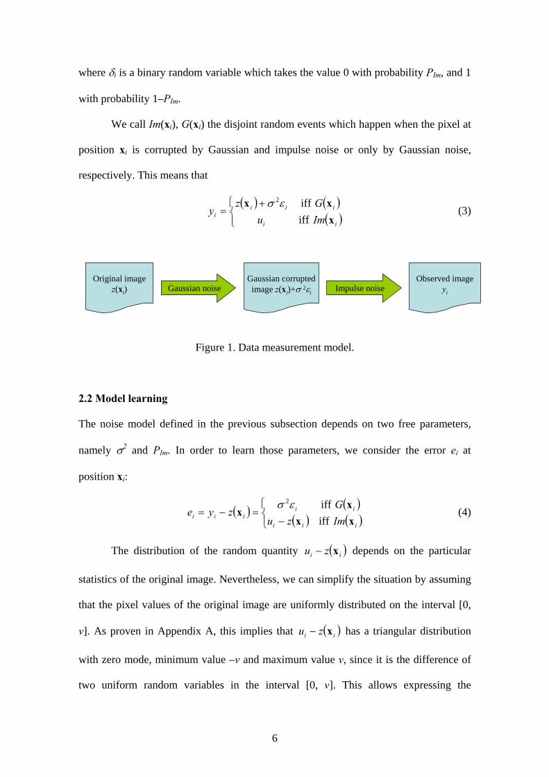
6
where δi is a binary random variable which takes the value 0 with probability PIm, and 1
with probability 1–PIm.
We call Im(xi), G(xi) the disjoint random events which happen when the pixel at
position xi is corrupted by Gaussian and impulse noise or only by Gaussian noise,
respectively. This means that
( ) ( )
( )⎩⎨⎧ +
=ii
iiii Imu
Gzy
xxx
iff iff2εσ
(3)
Original imagez(xi) Gaussian noise
Gaussian corruptedimage z(xi)+σ 2εi
Observed imageyiImpulse noise
Figure 1. Data measurement model.
2.2 Model learning
The noise model defined in the previous subsection depends on two free parameters,
namely σ2 and PIm. In order to learn those parameters, we consider the error ei at
position xi:
( ) ( )( ) ( )⎩
⎨⎧
−=−=
iii
iiiii Imzu
Gzye
xxx
x iff iff2εσ
(4)
The distribution of the random quantity ( )ii zu x− depends on the particular
statistics of the original image. Nevertheless, we can simplify the situation by assuming
that the pixel values of the original image are uniformly distributed on the interval [0,
v]. As proven in Appendix A, this implies that ( )ii zu x− has a triangular distribution
with zero mode, minimum value –v and maximum value v, since it is the difference of
two uniform random variables in the interval [0, v]. This allows expressing the

7
probability density of the error ei as a probabilistic mixture of a Gaussian density and a
triangular density:
( ) ( ) ( ) ( )ivImiImi eTriPeNPep +−= σ1 (5)
where the triangular probability density function (pdf) is
( )
⎪⎪⎪
⎩
⎪⎪⎪
⎨
⎧
≤≤−
≤≤−+
=
otherwise0
0if
0if
2
2
vev
ev
evv
ev
eTri ii
ii
iv (6)
and the Gaussian pdf is given by
( ) ⎟⎟⎠
⎞⎜⎜⎝
⎛−= 2
2
exp2
1σπσσ
ii
eeN (7)
To get a clearer picture of the situation, please see Figure 2, where the
conditional density functions of the error are shown.
-v 0 v0
p(0)
ei
p(e i |
G(x
i))
-v 0 v0
1/v
ei
p(e i |
Im(x
i))
Figure 2. Probability density function p(ei) of the error ei for non impulse corrupted
pixels (left) and impulse corrupted pixels (right).

8
A method is needed to estimate the free parameters σ2 and PIm from the errors ei
corresponding to the pixels of the image. In particular, we wish to obtain estimators
which maximize the data likelihood under the mixture model:
( ) ( )∑=i
ImiIm σ,Pepσ,PL |log (8)
This is accomplished by a specific version of the Expectation-Maximization
(EM) algorithm [40, 41], which is developed in Appendix B. The update equations for
each iteration t of the EM algorithm read:
( ) ∑=+i
tiImIm RAB
tP ,,11 (9)
( ) ( )( )111
2,,
+−=+
∑tPAB
eRt
Im
iitiG
σ (10)
where
( ) ( )( )( )tep
eTritPRi
ivImtiIm θ|,, = (11)
( )( ) ( ) ( )
( )( )tepeNtP
Ri
itImtiG θ
σ
|1
,,
−= (12)
and the iteration is continued until convergence.
There is an additional issue. The EM algorithm accepts the errors ei as inputs,
but these values are unknown. We propose to use another image restoration technique to
produce predictions of the pixel values ( )iz x~ , so that the predicted errors can be also
computed:
( )iii zye x~~ −= (13)
Finally, the error predictions ie~ are fed to the EM algorithm. The more accurate
the pixel predictions ( )iz x~ , the best estimators for the free parameters σ2 and PIm we
get. We have tested some image restoration techniques, and the Iteratively Reweighted

9
Norm (IRN) approach [30] has been found to work well for this purpose. Hence, we
have chosen it for the experiments. The IRN method is based on the minimization of a
functional which includes two terms. One of them measures the fidelity of the
reconstruction to the input image, and it depends on a weighted L2-norm of the
differences among the reconstructed and the original pixel values. The second term is
called the regularization term, and it penalizes reconstructed images with high gradient
values. This is aimed to reduce the noise, which is typically accompanied by sharp
changes in the pixel values. Then the Jacobian and the Hessian of the functional are
obtained, and finally the minimization is carried out by a variation of Newton’s method.
3 Kernel regression
3.1 Adaptive image restoration
In the classic 2D kernel regression framework, we would try to estimate ( )iz x as
the mean regression function of the observed data:
( ) ( ) [ ]iiiii yEzezy =⇒+= xx (14)
since [ ] 0=ieE . Here our alternative approach is to estimate ( )iz x as the mean
regression function of the non impulse-corrupted observed data:
( ) ( )[ ]iii GyEz xx |= (15)
Please note that, while the mean regression function to be estimated is the same
in both cases,
[ ] ( )[ ]iii GyEyE x|= (16)
the second option is more convenient, since the Gaussian noise variance σ2 is expected
to be lower than the variance of the combined (Gaussian and impulse) noise:
( )[ ] ( )[ ] 2|var|var σ== iiii GeGy xx (17)

10
[ ] [ ] ( )6
1varvar2
2 vPPey ImImii +−== σ (18)
[ ] ( )[ ]iii Gyy x|varvar > (19)
where [ ]ievar is obtained in Appendix C, and σ<<v. The above equation is the
mathematical expression of the following fact: impulse corrupted pixels do not carry
any information about the original image.
Let x∈[1,A]×[1,B] be a position on the image, which may or may not be
coincident with a pixel position, i.e., subpixel accuracy is allowed. The local kernel
estimator in the vicinity of x is given by
( ) ( ) ( )( ) ( ) ( ) ( )( )( ) ...21
+−−+−∇+= xxxxxxxxxx iT
iiT
i zzzz H (20)
where ∇ and H are the gradient and Hessian operators, respectively, and ( )iG x verifies,
i.e., the input pixel at position xi is Gaussian corrupted. If we take into account the
symmetry of the Hessian matrix, we may write
( ) ( ) ( )( )( ) ...svec210 +−−+−+= Tii
Ti
Tiz xxxxβxxβx β (21)
where svec(·) is a vectorization of a symmetric matrix,
( )Tcbacbba
=⎟⎟⎠
⎞⎜⎜⎝
⎛⎥⎦
⎤⎢⎣
⎡svec (22)
and the parameters to be determined are:
( )xz=0β (23)
( ) ( ) ( ) T
xz
xzz ⎥
⎦
⎤⎢⎣
⎡∂∂
∂∂
=∇=21
1 , xxxβ (24)
( ) ( ) ( ) T
xz
xxz
xz
⎥⎦
⎤⎢⎣
⎡
∂∂
∂∂
∂∂
= 22
2
21
2
21
2
2 ,2,21 xxxβ (25)
We group the parameters for notational convenience:

11
[ ]TT
NT ββb ,...,, 10β=
(26)
with N the order of the estimation.
Note that ( )xz=0β is the estimated image value at x. These parameters are
obtained by solving the following optimization problem, where only the Gaussian
corrupted pixels are considered:
( )bbb
Fminargˆ = (27)
( ) ( ) ( ) ( )( )( )[ ]∑ −−−−−−−−=i
Tii
Ti
Tiiii yKF
2
210 ...svec xxxxβxxβxxb βδ (28)
In the above equation iK is the 2D smoothing kernel function for pixel i, which
will be studied in the next subsection.
Since the value of the random variable δi for a pixel i is not known, that is,
whether i is Gaussian or impulse corrupted, objective function (28) can not be evaluated
directly. Instead of this, we substitute it by its expectation under the observed pixel
value yi, so the optimization problem to be solved in practice is
( ) ]|[minargˆ
iyFE bbb
= (29)
( ) =]|[ iyFE b
[ ] ( ) ( ) ( )( )( )[ ]∑ −−−−−−−−i
Tii
Ti
Tiiiii yKyE
2
210 ...svec| xxxxβxxβxx βδ (30)
The relevant expectations are computed by Bayes’ theorem:
[ ] ( )( ) ( )( ) ( )( )( )i
iiiiiiii ep
GepeGPyGPyE ~|~~||| xxx ===δ (31)
where the probability densities p come from the mixture model trained in Section 2, that
is, we are using the predicted errors for approximation:
( ) ( )ii epep ≈~ (32)
( )( ) ( )( )iiii GepGep xx ||~ ≈ (33)

12
Equation (31) can be rewritten by using (5) to yield a more explicit formulation:
[ ] ( )( ) ( ) ( )( ) ( ) ( )ivImiIm
iImiiii eTriPeNP
eNPyGPyE ~~1
~1||+−
−==
σ
σδ x (34)
Next we rewrite the problem (29) in matrix form:
( ) ( )bXyWbXybXyb xxxbWxb
x −−=−= Tminargminargˆ 2 (35)
where
( )TMyy ,...,1=y (36)
[ ] ( ) [ ] ( )[ ]xxxxWx −−= MMMM KyEKyE |,...,|diag 1111 δδ (37)
( ) ( )( )( )( ) ( )( )( )
( ) ( )( )( ) ⎥⎥⎥⎥⎥
⎦
⎤
⎢⎢⎢⎢⎢
⎣
⎡
−−−
−−−−−−
=
...svec1
...svec1
...svec1
222
111
TMM
TTM
TTT
TTT
xxxxxx
xxxxxxxxxxxx
XxMMMM
(38)
with ‘diag’ producing a diagonal matrix, and M being the number of pixels in a suitable
neighbourhood V of position x. This facilitates to obtain its solution by standard
weighted least squares theory ([42, 43]):
( ) yWXXWXb xxxxxTT 1ˆ −
= (39)
provided that xxx XWX T is invertible. In our experiments, V has been chosen to
comprise the pixels in a circle with fixed radius r, centred in x.
3.2 Adaptive kernel estimation
The adaptation to the input data is enhanced if we choose the 2D smoothing
kernel Ki to depend on the local gradient covariance matrix Ci (see [13]):
( ) ( ) ( ) ( )⎟⎠⎞
⎜⎝⎛ −−−=− xxCxx
Cxx ii
Ti
iii hh
K 22 21exp
2detπ
(40)
where h is a global smoothing parameter and Ci is given by (see [44]):
13
( )( ) ( )( )i
Ti zz xxC ∇∇= (41)
( ) ( )∫∫=iV
idxxζxζ (42)
with Vi a local neighbourhood of pixel xi. Like before, in practice Vi is a circle with
fixed radius r, centred in xi.
In order to estimate Ci, Takeda et al. [13] proposed to compute the truncated
singular value decomposition (SVD) of the local gradient matrix Gi:
( )( ) iT
iiiT
ji Vjz ∈=⎟⎟⎟
⎠
⎞
⎜⎜⎜
⎝
⎛∇= with,
...
...VSUxG (43)
where Si is a 2x2 diagonal matrix representing the energy in the dominant directions,
and Vi is a 2x2 orthogonal matrix whose second column (ν1, ν2)T defines the dominant
orientation angle θi:
⎟⎟⎠
⎞⎜⎜⎝
⎛=
2
1arctanννθ i (44)
The local elongation parameter ρi is computed from the diagonal elements s1, s2
of Si:
''
2
1
λλρ
++
=ss
i (45)
where λ’≥0 is a regularization parameter. The local scaling parameter γi is given by:
M
ssi
''21 λγ += (46)
where λ’’≥0 is another regularization parameter, and M stands for the number of pixels
in the local neighbourhood Vi.
Then, the local gradient covariance matrix estimator iC , which we will only use
for Gaussian corrupted pixels, is obtained as follows:
14
( ) Ti
i
iiiiiG ΘΘCx ⎟⎟
⎠
⎞⎜⎜⎝
⎛=⇒ −10
0ˆρ
ργ (47)
⎟⎟⎠
⎞⎜⎜⎝
⎛−
=ii
iii θθ
θθcossinsincos
Θ (48)
Careful estimation of Ci is of paramount importance for kernel regression in our
context, because impulse corrupted pixels may introduce considerable errors. To take
this into account, we consider that the best estimation of Ci for an impulse corrupted
pixel is the null matrix, which corresponds to a locally constant image:
( ) 0Cx =⇒ iiIm ˆ (49) Hence, the estimator iC for an arbitrary pixel is derived from (47) and (49):
Ti
i
iiiii ΘΘC ⎟⎟
⎠
⎞⎜⎜⎝
⎛= −10
0ˆρ
ργδ (50)
As in the previous subsection, the above equation can not be implemented
directly, since we do not know whether a particular pixel i is Gaussian or impulse
corrupted. Hence, in practice we use the expectation of iC under the observed pixel
value yi:
[ ] [ ] Ti
i
iiiiiii yEyE ΘΘC ⎟⎟
⎠
⎞⎜⎜⎝
⎛= −10
0||ˆ
ρρ
γδ (51)
where [ ]ii yE |δ is obtained from (34), as before.
3.3 Algorithm
In this subsection we specify how the above presented techniques can be
combined in order to develop a restoration algorithm.

15
The first stage involves obtaining the pixel predictions ( )iz x~ from IRN or any
other suitable method, so that the noise model can be learnt by the EM algorithm
(subsection 2.2).
Then we execute a preliminary kernel regression. As the gradient is not known,
we take
[ ] [ ] ⎟⎟⎠
⎞⎜⎜⎝
⎛=
1111
||ˆiiii yEyE δC (52)
as a first approach. This produces preliminary estimators of the gradient ( )xz∇ , which
we use to compute [ ]ii yE |C more accurately, by means of the procedure explained in
subsection 3.2.
Finally, these more accurate values of [ ]ii yE |C are fed into the kernel
regression to yield the definitive restored image.
Hence, the algorithm is as follows:
1. Execute the IRN method (or any other) on the input image to yield
predictions ( )iz x~ of the original pixel values, and compute the
corresponding predicted errors ie~ by equation (13).
2. Train the noise model by the EM algorithm, equations (9)-(10), until
convergence. The input samples ei for this algorithm are approximated by the
predicted errors ie~ obtained in Step 1.
3. Perform a preliminary kernel regression, equation (39), where the local
gradient covariance matrices Ci are tentatively approximated by the
expectations [ ]ii yE |C in equation (52). This regression produces
preliminary approximations of the gradient ( )xz∇ .
16
4. Find more accurate approximations of the local gradient covariance matrices
from equation (51), where the necessary gradient approximations come from
the output of Step 3.
5. Perform the final kernel regression, equation (39), where the local gradient
covariance matrices Ci are approximated by the expectations [ ]ii yE |C
obtained in Step 4.
It must be noted that the above algorithm not only produces the restored image
values from equation (23), but also estimates the gradient from equation (24). In order
to apply it to colour images, it must be taken into account that in image coding schemes
used in practice there is one colour component which is coded with more spatial
resolution, namely that which carries the luminosity information. Hence, we always
estimate the local gradient from that component, while the kernel regression is
performed separately on each component.
As our approach is aimed to restore very noisy images, we call it Heavily
Damaged Image Restoration (HDIR).
4 Discussion
Our method can be conceived as a combination of noise mixture modelling with
kernel regression, which is designed to remove two kinds of noise occurring in the same
image. Hence it departs from previously known methods, although it shares several
properties with some of them. Next we consider those approaches which have
something in common with ours.
a) Impulse noise removers [45, 21, 22, 46] assume that the erroneous pixels
differ significantly from their neighbours. We take this general hypothesis
17
one step further by defining a probabilistic noise model. This allows
exploiting the particular statistical properties of its randomness in full, and
provides a framework to distinguish impulses from Gaussian corrupted
pixels in a principled way.
b) Kernel regression methods [12, 13] suppose that there is an underlying
function whose values are corrupted by some process to yield the observed
values. In principle they do not assume any probability distribution for this
noise process [42]. Our strategy adds a mixture noise model to this
framework, so as to improve its performance by considering each input pixel
in light of its likelihood of carrying useful information.
c) Many wavelet shrinkage methods use statistical models of either the original
image or the corrupted one [14, 15]. This is the equivalent in the wavelet
domain of our probabilistic noise model. In particular, Luisier et al. [16] use
Stein’s Unbiased Risk Estimation (SURE) to avoid a statistical model for the
wavelet coefficients. The relations between SURE and kernel regression
have been studied in [47]. On the other hand, Pizurica and Philips [17]
estimate the probability that a certain wavelet coefficient contains a
significant noise-free component, much like our estimation of the probability
that a given pixel is not impulse corrupted. In spite of these similarities and
connections, HDIR is fundamentally different from all of them, since these
methods work on the wavelet coefficients, while our proposal works directly
on the pixel values.
18
5 Experimental results
Given the wide range of image restoration methods currently available, we have
selected 9 of them which belong to very different approaches to this problem. Next we
list them, along with the abbreviation used in the following figures and their most
outstanding features:
a) Iteratively Reweighted Norm, IRN [30]. As mentioned before, it is a total
variation regularization approach which minimizes a functional that takes
into account both the fidelity to the input data and the smoothness of the
solution.
b) Iterative Steering Kernel Regression, ISKR [13]. This is a state-of-the-art
kernel regression method. It performs several kernel regressions iteratively,
so that the noise is progressively removed. On each iteration the local
orientation is estimated, so as not to affect the edges of the original image.
c) Progressive Switching Median Filter, PSMF [48]. It has two modules: an
impulse detector and a restoring filter, both based on the median as a robust
statistic. The filter is applied to a pixel only if an impulse is detected, i.e., it
is switched on and off.
d) Decision-Based Algorithm for Removal of High-Density Impulse Noises,
DBAIN [49]. This algorithm is oriented to removing impulse corrupted pixel
with extreme values (salt-and-pepper), i.e., either 0 or v. Hence, it is not
designed for the kinds of noise we are considering here, but we include it as
an illustration of what happens when it faces non extreme values.
e) NeighShrink-SURE, NS [14]. This is a wavelet shrinkage method that
determines an optimal threshold and neighbouring window size for every
wavelet subband by the Stein’s unbiased risk estimate (SURE).

19
f) Interscale Orthonormal Wavelet Thresholding, OWT [16]. It is also a SURE-
based wavelet shrinkage approach. It parametrizes the denoising process as a
sum of elementary nonlinear processes with unknown weights, and does
need not hypothesize a statistical model for the original image.
g) BiShrink Wavelet-Based Denoising using the Separable Discrete Wavelet
Transform, BiS [15]. This method uses a bivariate shrinkage function which
models the statistical dependence between a wavelet coefficient and its
parent.
h) BiShrink Wavelet-Based Denoising using the Dual-Tree Discrete Wavelet
Transform, BiS2 [15]. It is analogous to the previous method, but with a
different wavelet transform.
i) ProbShrink, PS [17]. It estimates the probability that a given wavelet
coefficient contains a significant noise-free component, and then the
coefficient is multiplied by that probability.
We have selected three benchmark images from the University of Waterloo
repertoire [50], which are shown in Figure 3. One of them (boat) is a 512×512 grayscale
image, and the other two (Lena and tulips) are colour images of sizes 512×512 and
768×512, respectively. For the colour images all the computations have been performed
on the Y’CbCr colour space, since it is widely used in practice to transmit colour
information, as done in JPEG image files [51] and MPEG video files [52]. In all cases
(grayscale and colour) the pixel values lie in the range [0,255], i.e. we have v=255.

20
Figure 3. Original images. From left to right: boat, Lena and tulips.
We have chosen as a quantitative restoration quality measure the Root Mean
Squared Error [13] (RMSE, lower is better):
( )∑=
−=AB
iii yy
ABRMSE
1
2ˆ1 (53)
For colour images, we average the squared error over all the spectral channels
(see for example [17, 53]). The RMSE has the same dimensions as the pixel values,
which in our case implies that RMSE∈[0,255] . Furthermore, it ranks any compared
methods in the same way as the Mean Squared Error (MSE, lower is better) and the
Peak Signal-to-Noise Ratio (PSNR, higher is better):
( )∑=
−=AB
iii yy
ABMSE
1
2ˆ1 (54)
MSE
PSNR2
10255log10= (55)
We have tested four different Gaussian noise levels: σ=15, 20, 25, 30. For each
value of the Gaussian noise standard deviation σ we have tested all the possible
proportions of impulse noise Pim between 0 and 0.4, in 0.05 increments. The results are
shown in Figures 4, 5 and 6 for boat, Lena and tulips, respectively. Our HDIR approach
yields the best results, followed by IRN, ISKR and some wavelet shrinkage methods
(BiS, BiS2 and PS). In particular, IRN minimizes a functional which has a term to
represent the fidelity to the input (noisy) image. This term takes into account all input
pixels, no matter how noisy they are. Hence, highly noisy pixels can affect the
restoration very negatively. On the other hand, HDIR discards the pixels with high noise
levels by assigning them a very small weight, i.e. [ ] 0| ≈ii yE δ in equation (30). This
means that the restoration is not affected by those pixels.

21
The performance of the PSMF method is very dependent on the features of the
input image, and degrades quickly as we increase the Gaussian noise level, which is due
to its orientation to impulse noise removal. On the other hand, the DBAIN method does
not reduce the error (the RMSE remains nearly the same as in the input image), as it is
designed to remove only extreme impulses.
0 0.05 0.1 0.15 0.2 0.25 0.3 0.35 0.40
10
20
30
40
50
60
70
80
Proportion of impulse corrupted pixels, Pim
RM
SE
InputHDIRIRNISKRPSMFDBAINNSOWTBiSBiS2PS
0 0.05 0.1 0.15 0.2 0.25 0.3 0.35 0.40
10
20
30
40
50
60
70
80
Proportion of impulse corrupted pixels, Pim
RM
SE
InputHDIRIRNISKRPSMFDBAINNSOWTBiSBiS2PS
0 0.05 0.1 0.15 0.2 0.25 0.3 0.35 0.40
10
20
30
40
50
60
70
80
Proportion of impulse corrupted pixels, Pim
RM
SE
InputHDIRIRNISKRPSMFDBAINNSOWTBiSBiS2PS
0 0.05 0.1 0.15 0.2 0.25 0.3 0.35 0.40
10
20
30
40
50
60
70
80
Proportion of impulse corrupted pixels, Pim
RM
SE
InputHDIRIRNISKRPSMFDBAINNSOWTBiSBiS2PS
Figure 4. Results for the boat image. From left to right and from top to bottom: RMSE
with Gaussian noise standard deviation σ=15, 20, 25, 30.

22
0 0.05 0.1 0.15 0.2 0.25 0.3 0.35 0.40
10
20
30
40
50
60
70
80
90
100
Proportion of impulse corrupted pixels, Pim
RM
SE
InputHDIRIRNISKRPSMFDBAINNSOWTBiSBiS2PS
0 0.05 0.1 0.15 0.2 0.25 0.3 0.35 0.40
10
20
30
40
50
60
70
80
90
100
Proportion of impulse corrupted pixels, Pim
RM
SE
InputHDIRIRNISKRPSMFDBAINNSOWTBiSBiS2PS
0 0.05 0.1 0.15 0.2 0.25 0.3 0.35 0.40
10
20
30
40
50
60
70
80
90
100
Proportion of impulse corrupted pixels, Pim
RM
SE
InputHDIRIRNISKRPSMFDBAINNSOWTBiSBiS2PS
0 0.05 0.1 0.15 0.2 0.25 0.3 0.35 0.40
10
20
30
40
50
60
70
80
90
100
Proportion of impulse corrupted pixels, Pim
RM
SE
InputHDIRIRNISKRPSMFDBAINNSOWTBiSBiS2PS
Figure 5. Results for the Lena image. From left to right and from top to bottom: RMSE
with Gaussian noise standard deviation σ=15, 20, 25, 30.
0 0.05 0.1 0.15 0.2 0.25 0.3 0.35 0.40
10
20
30
40
50
60
70
80
90
100
110
Proportion of impulse corrupted pixels, Pim
RM
SE
InputHDIRIRNISKRPSMFDBAINNSOWTBiSBiS2PS
0 0.05 0.1 0.15 0.2 0.25 0.3 0.35 0.40
10
20
30
40
50
60
70
80
90
100
110
Proportion of impulse corrupted pixels, Pim
RM
SE
InputHDIRIRNISKRPSMFDBAINNSOWTBiSBiS2PS
23
0 0.05 0.1 0.15 0.2 0.25 0.3 0.35 0.40
10
20
30
40
50
60
70
80
90
100
110
Proportion of impulse corrupted pixels, Pim
RM
SE
InputHDIRIRNISKRPSMFDBAINNSOWTBiSBiS2PS
0 0.05 0.1 0.15 0.2 0.25 0.3 0.35 0.40
10
20
30
40
50
60
70
80
90
100
110
Proportion of impulse corrupted pixels, Pim
RM
SE
InputHDIRIRNISKRPSMFDBAINNSOWTBiSBiS2PS
Figure 6. Results for the tulips image. From left to right and from top to bottom: RMSE
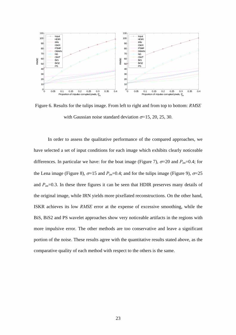
with Gaussian noise standard deviation σ=15, 20, 25, 30.
In order to assess the qualitative performance of the compared approaches, we
have selected a set of input conditions for each image which exhibits clearly noticeable
differences. In particular we have: for the boat image (Figure 7), σ=20 and Pim=0.4; for
the Lena image (Figure 8), σ=15 and Pim=0.4; and for the tulips image (Figure 9), σ=25
and Pim=0.3. In these three figures it can be seen that HDIR preserves many details of
the original image, while IRN yields more pixellated reconstructions. On the other hand,
ISKR achieves its low RMSE error at the expense of excessive smoothing, while the
BiS, BiS2 and PS wavelet approaches show very noticeable artifacts in the regions with
more impulsive error. The other methods are too conservative and leave a significant
portion of the noise. These results agree with the quantitative results stated above, as the
comparative quality of each method with respect to the others is the same.

24
Figure 7. Detail of the boat image. From left to right and from top to bottom (RMSE in
parentheses): Original image, corrupted image (57.1502), HDIR (15.1001), IRN
(19.7459), ISKR (25.4810), PSMF (22.3838), DBAIN (57.2077), NS (51.2987), OWT
(51.2987), BiS (25.6406), BiS2 (24.7716), PS (24.5345).

25
Figure 8. Detail of the Lena image. From left to right and from top to bottom (RMSE in
parentheses): Original image, corrupted image (90.5691), HDIR (12.3469), IRN
(19.5763), ISKR (27.8849), PSMF (28.5702), DBAIN (90.5600), NS (84.2008), OWT
(83.5118), BiS (28.2878), BiS2 (27.2574), PS (28.4346).

26
Figure 9. Detail of the tulips image. From left to right and from top to bottom (RMSE in
parentheses): Original image, corrupted image (87.5721), HDIR (17.1924), IRN
(22.8797), ISKR (29.9664), PSMF (32.8684), DBAIN (87.5431), NS (69.4079), OWT
(67.9032), BiS (31.4287), BiS2 (29.8594), PS (31.0968).
27
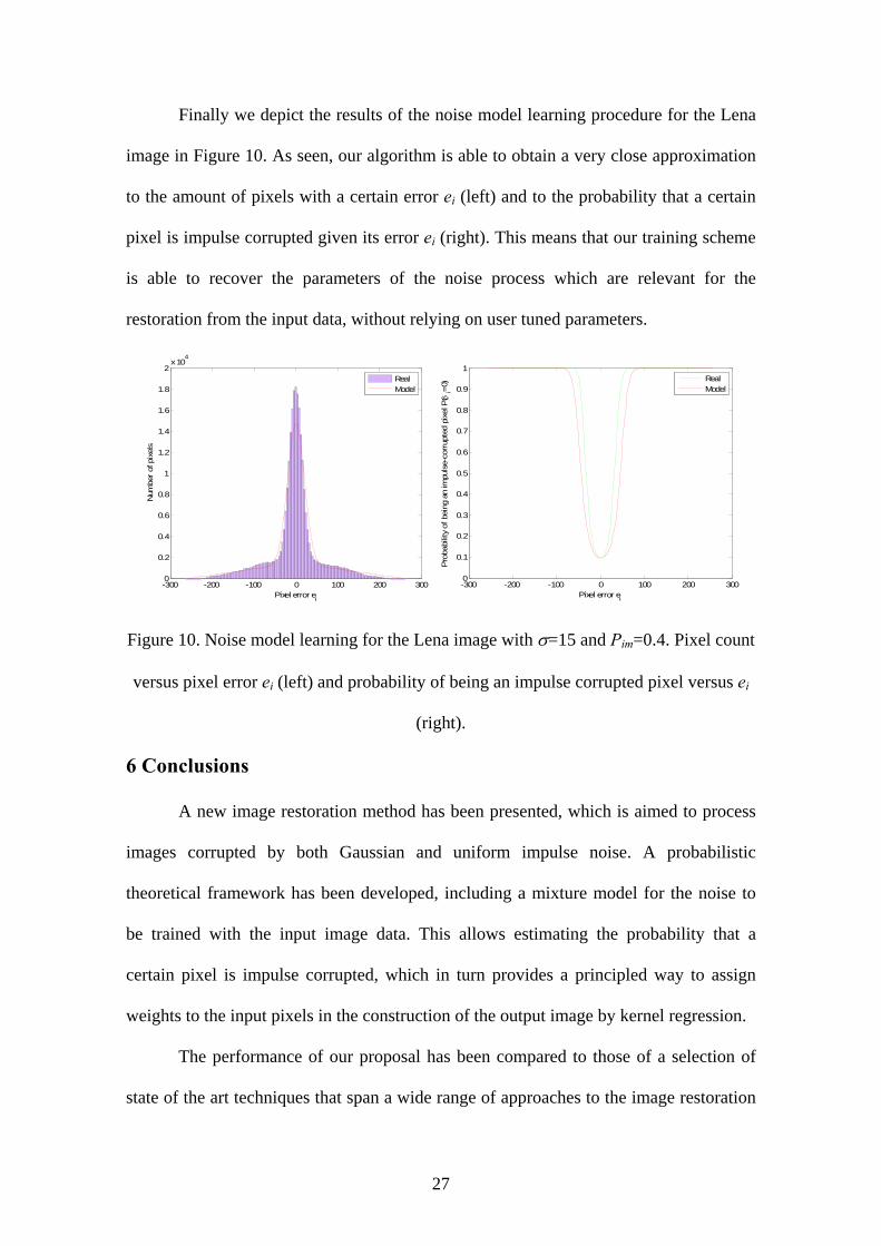
Finally we depict the results of the noise model learning procedure for the Lena
image in Figure 10. As seen, our algorithm is able to obtain a very close approximation
to the amount of pixels with a certain error ei (left) and to the probability that a certain
pixel is impulse corrupted given its error ei (right). This means that our training scheme
is able to recover the parameters of the noise process which are relevant for the
restoration from the input data, without relying on user tuned parameters.
-300 -200 -100 0 100 200 3000
0.2
0.4
0.6
0.8
1
1.2
1.4
1.6
1.8
2x 10
4
Pixel error ei
Num
ber
of p
ixel
s
RealModel
-300 -200 -100 0 100 200 3000
0.1
0.2
0.3
0.4
0.5
0.6
0.7
0.8
0.9
1
Pixel error ei
Pro
babi
lity
of b
eing
an
impu
lse-
corr
upte
d pi
xel P
( δ i=
0)
RealModel
Figure 10. Noise model learning for the Lena image with σ=15 and Pim=0.4. Pixel count
versus pixel error ei (left) and probability of being an impulse corrupted pixel versus ei
(right).
6 Conclusions
A new image restoration method has been presented, which is aimed to process
images corrupted by both Gaussian and uniform impulse noise. A probabilistic
theoretical framework has been developed, including a mixture model for the noise to
be trained with the input image data. This allows estimating the probability that a
certain pixel is impulse corrupted, which in turn provides a principled way to assign
weights to the input pixels in the construction of the output image by kernel regression.
The performance of our proposal has been compared to those of a selection of
state of the art techniques that span a wide range of approaches to the image restoration
28
problem. The quantitative and qualitative results with benchmark images show that our
method removes the noise while it preserves the fine details of the original image.
Acknowledgements
This work was partially supported by the Ministry of Education and Science of
Spain under Project TIN2006-07362, and by the Autonomous Government of Andalusia
(Spain) under Projects P06-TIC-01615 and P07-TIC-02800.
Appendix A: Distribution of the error for impulse corrupted pixels
Let z(xi), yi be the original and observed pixel values at position xi, which is
affected by impulse noise. Then both random variables are uniform in the interval [0, v].
The probability density function of yi is:
( )⎪⎩
⎪⎨⎧ ≤≤
=otherwise0
0iff1 vavaf (56)
The probability density function of –z(xi) is:
( )⎪⎩
⎪⎨⎧ ≤≤−
=otherwise0
0iff1 avvag (57)
Now we compute the probability density function of their sum ei as the
convolution of f and g:
( ) ( )( ) ( ) ( )∫∞
∞−
−== iiiiii dyygyefegfep * (58)
From the definition of g we get:
( ) ( )∫−
−=01
viiii dyyef
vep (59)

29
Now the integrand is zero unless vye ii ≤−≤0 , and then it is 1/v. Hence,
( ) 2
0 110v
evdyvv
epve i
veiii
i
−==⇒≤≤ ∫
−
(60)
On the other hand,
( ) 2110
vevdy
vvepev i
e
viii
i +==⇒≤≤− ∫
−
(61)
And finally,
[ ] ( ) 0, =⇒−∉ ii epvve (62)
So we arrive at the triangular density with zero mode, minimum value –v and
maximum value v:
( ) ( )
⎪⎪⎪
⎩
⎪⎪⎪
⎨
⎧
≤≤−
≤≤−+
==
otherwise0
0if
0if
2
2
vev
ev
evv
ev
eTriep ii
ii
ivi (63)
Appendix B: Model learning with the Expectation-maximization
algorithm
We must maximize the data likelihood,
( ) ( )∑=i
ImiIm σ,Pepσ,PL |log (64)
where
( ) ( ) ( ) ( )ivImiImImi eTriPeNPσ,Pep +−= σ1| (65)
The parameter approximations at time step t are grouped in a parameter vector
θ(t):
( ) ( ) ( )( )t,Ptσt Im=θ (66)

30
For the E step, first we compute the posterior probability of the mixture
components for having generated the sample ei:
( ) ( )( ) ( ) ( )( )( )tep
eTritPRteImPi
ivImtiImii θ
θ|
,| ,, ==x (67)
( ) ( )( ) ( )( ) ( )( )( )( )tep
eNtPRteGP
i
itImtiGii θ
θ σ
|1
,| ,,
−==x (68)
Then we obtain the expectation of the likelihood:
( )[ ] ( ) ( )( ) ( )( ) ( )( )( )∑ +−++=i
iImtiGivImtiIm eNtPReTritPRLE σθ log1logloglog ,,,, (69)
For the M step, both parameters may be optimized independently, since they
appear in (69) in separate linear terms.
First we consider PIm:
( ) ( )⎭⎬⎫
⎩⎨⎧
−⎟⎠
⎞⎜⎝
⎛+⎟
⎠
⎞⎜⎝
⎛=+ ∑∑ αα
α1loglogmaxarg1 ,,,,
itiG
itiImIm RRtP (70)
This is analogous to the maximum likelihood estimator for the binomial
distribution, so we have:
( ) ∑∑∑∑
=+
=+i
tiIm
itiG
itiIm
itiIm
Im RABRR
RtP ,,
,,,,
,, 11 (71)
On the other hand,
( ) ( )∑=+i
itiG eNRt αµασ ,,, logmaxarg1 (72)
This is analogous to the weighted maximum likelihood estimator of a normal
distribution, so we get:
( ) ( )( )111
2,,
,,
2,,
+−==+
∑∑∑
tPAB
eR
R
eRt
Im
iitiG
itiG
iitiG
σ (73)

31
Being an EM algorithm, it is guaranteed that these equations converge to a
maximum of the likelihood L (see for example [54]).
Appendix C: Noise variance
Here we are interested in the noise variance, [ ]ievar . Since the noise has zero
mean, we have:
[ ] [ ][ ] [ ]22var iiii eEeEeEe =−= (74)
Since every pixel i is either Gaussian or impulse corrupted,
[ ] ( )( ) ( )[ ] ( )( ) ( )[ ]iiiiiii ImeEImPGeEGPe xxxx ||var 22 += (75)
We rewrite in terms of ( )( )iIm ImPP x= :
[ ] ( ) ( )[ ] ( )[ ]iiImiiImi ImeEPGeEPe xx ||1var 22 +−= (76)
Finally, we use the variance of the triangular distribution (see [55, 56]) to yield:
[ ] ( )6
1var2
2 vPPe ImImi +−= σ (77)
References
[1] M. Ben-Ezra, S. K. Nayar, Motion-based motion deblurring, IEEE Transactions
on Pattern Analysis and Machine Intelligence 26 (6) (2004) 689–698.
[2] S. Schuon, K. Diepold, Comparison of motion de-blur algorithms and real world
deployment, Acta Astronautica 64 (11-12) (2009) 1050 – 1065.
[3] B.-D. Choi, S.-W. Jung, S.-J. Ko, Motion-blur-free camera system splitting
exposure time, IEEE Transactions on Consumer Electronics 54 (3) (2008) 981–
986.

32
[4] T. Shin, J.-F. Nielsen, K. Nayak, Accelerating dynamic spiral MRI by algebraic
reconstruction from undersampled k-t space, IEEE Transactions on Medical
Imaging 26 (7) (2007) 917–924.
[5] J. Zhang, Q. Zhang, G. He, Blind deconvolution of a noisy degraded image,
Applied Optics 48 (12) (2009) 2350–2355.
[6] H. Rabbani, Image denoising in steerable pyramid domain based on a local
Laplace prior, Pattern Recognition 42 (9) (2009) 2181 – 2193.
[7] F. Russo, A method for estimation and filtering of Gaussian noise in images,
IEEE Transactions on Instrumentation and Measurement 52 (4) (2003) 1148–
1154.
[8] M. Ghazal, A. Amer, A. Ghrayeb, Structure-oriented multidirectional Wiener
filter for denoising of image and video signals, IEEE Transactions on Circuits
and Systems for Video Technology 18 (12) (2008) 1797–1802.
[9] A. C. Bovik, Handbook of Image and Video Processing (Communications,
Networking and Multimedia), Academic Press, Inc., Orlando, FL, USA, 2005.
[10] M. Figueiredo, J. Bioucas-Dias, R. Nowak, Majorization–minimization
algorithms for wavelet-based image restoration, IEEE Transactions on Image
Processing 16 (12) (2007) 2980–2991.
[11] V. Bruni, D. Vitulano, Combined image compression and denoising using
wavelets, Signal Processing: Image Communication 22 (1).
[12] J.-S. Zhang, X.-F. Huang, C.-H. Zhou, An improved kernel regression method
based on Taylor expansion, Applied Mathematics and Computation 193 (2)
(2007) 419 – 429.
[13] H. Takeda, S. Farsiu, P. Milanfar, Kernel regression for image processing and
reconstruction, IEEE Transactions on Image Processing 16 (2) (2007) 349–366.

33
[14] Z. Dengwen, C. Wengang, Image denoising with an optimal threshold and
neighbouring window, Pattern Recognition Letters 29 (11) (2008) 1694 – 1697.
[15] L. Sendur, I. Selesnick, Bivariate shrinkage with local variance estimation, IEEE
Signal Processing Letters 9 (12) (2002) 438–441.
[16] F. Luisier, T. Blu, M. Unser, A new SURE approach to image denoising:
Interscale orthonormal wavelet thresholding, Image Processing, IEEE
Transactions on 16 (3) (2007) 593–606.
[17] A. Pizurica, W. Philips, Estimating the probability of the presence of a signal of
interest in multiresolution single- and multiband image denoising, IEEE
Transactions on Image Processing 15 (3) (2006) 654–665.
[18] N. Alajlan, M. Kamel, E. Jernigan, Detail preserving impulsive noise removal,
Signal Processing: Image Communication 19 (10) (2004) 993 – 1003.
[19] H. Kong, L. Guan, A neural network adaptive filter for the removal of impulse
noise in digital images, Neural Networks 9 (3) (1996) 373 – 378.
[20] W. Luo, An efficient detail-preserving approach for removing impulse noise in
images, IEEE Signal Processing Letters 13 (7) (2006) 413–416.
[21] C.-C. Kang, W.-J. Wang, Fuzzy reasoning-based directional median filter
design, Signal Processing 89 (3) (2009) 344 – 351.
[22] S.-S. Wang, C.-H. Wu, A new impulse detection and filtering method for
removal of wide range impulse noises, Pattern Recognition 42 (9) (2009) 2194 –
2202.
[23] R. Lukac, Adaptive vector median filtering, Pattern Recognition Letters 24 (12)
(2003) 1889–1899.
34
[24] E. Besdok, A new method for impulsive noise suppression from highly distorted
images by using Anfis, Engineering Applications of Artificial Intelligence 17 (5)
(2004) 519 – 527.
[25] R.-S. Lin, Y.-C. Hsueh, Multichannel filtering by gradient information, Signal
Processing 80 (2) (2000) 279 – 293.
[26] C. Liu, R. Szeliski, S. B. Kang, C. L. Zitnick, W. T. Freeman, Automatic
estimation and removal of noise from a single image, IEEE Transactions on
Pattern Analysis and Machine Intelligence 30 (2) (2008) 299–314.
[27] H. Ibrahim, N. Kong, T. F. Ng, Simple adaptive median filter for the removal of
impulse noise from highly corrupted images, IEEE Transactions on Consumer
Electronics 54 (4) (2008) 1920–1927.
[28] A. Gabay, M. Kieffer, P. Duhamel, Joint source-channel coding using real BCH
codes for robust image transmission, IEEE Transactions on Image Processing
16 (6) (2007) 1568–1583.
[29] G. Redinbo, Decoding real block codes: activity detection Wiener estimation,
IEEE Transactions on Information Theory 46 (2) (2000) 609–623.
[30] P. Rodriguez, B. Wohlberg, Efficient minimization method for a generalized
total variation functional, IEEE Transactions on Image Processing 18 (2) (2009)
322–332.
[31] L. Bar, A. Brook, N. Sochen, N. Kiryati, Deblurring of color images corrupted
by impulsive noise, IEEE Transactions on Image Processing 16 (4) (2007)
1101–1111.
[32] A. Bovik, T. Huang, J. Munson, D., A generalization of median filtering using
linear combinations of order statistics, IEEE Transactions on Acoustics, Speech
and Signal Processing 31 (6) (1983) 1342–1350.

35
[33] H. Yu, L. Zhao, H. Wang, An efficient procedure for removing random-valued
impulse noise in images, IEEE Signal Processing Letters 15 (2008) 922–925.
[34] A fast efficient restoration algorithm for high-noise image filtering with adaptive
approach, Journal of Visual Communication and Image Representation 16 (3)
(2005) 379 – 392.
[35] Noise reduction in high dynamic range imaging, Journal of Visual
Communication and Image Representation 18 (5) (2007) 366 – 376, special
issue on High Dynamic Range Imaging.
[36] T. Rabie, Adaptive hybrid mean and median filtering of high-iso long-exposure
sensor noise for digital photography, Journal of Electronic Imaging 13 (2)
(2004) 264–277.
[37] I. Inoue, N. Tanaka, H. Yamashita, T. Yamaguchi, H. Ishiwata, H. Ihara, Low-
leakage-current and low-operating-voltage buried photodiode for a CMOS
imager, IEEE Transactions on Electron Devices 50 (1) (2003) 43–47.
[38] R. Garnett, T. Huegerich, C. Chui, W. He, A universal noise removal algorithm
with an impulse detector, IEEE Transactions on Image Processing 14 (11)
(2005) 1747–1754.
[39] L. Ji, Z. Yi, A mixed noise image filtering method using weighted-linking
PCNNs, Neurocomputing 71 (13-15) (2008) 2986 – 3000.
[40] R. V. Hogg, A. Craig, J. W. McKean, Introduction to Mathematical Statistics
(6th Edition), Prentice Hall, 2004.
[41] T. Hastie, R. Tibshirani, J. H. Friedman, The Elements of Statistical Learning
(2nd Edition), Springer, 2009.
[42] M. P. Wand, M. C. Jones, Kernel Smoothing (Monographs on Statistics and
Applied Probability), Chapman & Hall/CRC, 1994.

36
[43] S. M. Kay, Fundamentals of Statistical Signal Processing, Volume I: Estimation
Theory, Prentice Hall PTR, 1993.
[44] S. Ando, Image field categorization and edge/corner detection from gradient
covariance, IEEE Transactions on Pattern Analysis and Machine Intelligence
22 (2) (2000) 179–190.
[45] Y. X. C. G. Chen, S., Impulse noise suppression with an augmentation of
ordered difference noise detector and an adaptive variational method, Pattern
Recognition Letters 30 (4) (2009) 460–467.
[46] D. E. P. K. Agaian, S.S., Logical system representation of images and removal
of impulse noise, IEEE Transactions on Systems, Man, and Cybernetics Part
A:Systems and Humans 38 (6) (2008) 1349–1362.
[47] D. N. G. Dinuzzo, F., An algebraic characterization of the optimum of
regularized kernel methods, Machine Learning 74 (3) (2009) 315–345.
[48] Z. Wang, D. Zhang, Progressive switching median filter for the removal of
impulse noise, IEEE Transactions on Circuits and Systems 46 (1) (1999) 78–80.
[49] K. S. Srinivasan, D. Ebenezer, A new fast and efficient decision-based algorithm
for removal of high-density impulse noises, IEEE Signal Processing Letters
14 (3) (2007) 189–192.
[50] University of Waterloo repertoire of images, In Internet:
http://links.uwaterloo.ca/colorset.base.html (2008).
[51] E. Hamilton, JPEG File Interchange Format (Version 1.02), C-Cube
Microsystems, 1992.
[52] T. Sikora, MPEG digital video coding standards, IEEE Signal Processing
Magazine 14 (1997) 82–100.

37
[53] E. López-Rubio, J. M. Ortiz-de-Lazcano-Lobato, D. López-Rodríguez,
Probabilistic PCA self-organizing maps, IEEE Transactions on Neural Networks
20 (9) (2009) 1474–1489.
[54] C. M. Bishop, Pattern Recognition and Machine Learning (Information Science
and Statistics), Springer, 2006.
[55] M. Evans, N. Hastings, B. Peacock, Statistical Distributions (3rd Edition),
Wiley, New York, 2000.
[56] R. N. Kacker, J. F. Lawrence, Trapezoidal and triangular distributions for Type
B evaluation of standard uncertainty, Metrologia 44 (2) (2007) 117–127.