response-surface methods in r, using rsmdk.archive.ubuntu.com/.../rsm/vignettes/rsm.pdf ·...
TRANSCRIPT

Response-Surface Methods in R, Using rsmUpdated to version 2.00, 5 December 2012
Russell V. LenthThe University of Iowa
Abstract
This introduction to the R package rsm is a modified version of Lenth (2009), pub-lished in the Journal of Statistical Software. The package rsm was designed to provideR support for standard response-surface methods. Functions are provided to generatecentral-composite and Box-Behnken designs. For analysis of the resulting data, the pack-age provides for estimating the response surface, testing its lack of fit, displaying an en-semble of contour plots of the fitted surface, and doing follow-up analyses such as steepestascent, canonical analysis, and ridge analysis. It also implements a coded-data structureto aid in this essential aspect of the methodology. The functions are designed in hopesof providing an intuitive and effective user interface. Potential exists for expanding thepackage in a variety of ways.
Keywords: response-surface methods, regression, experimental design, first-order designs,second-order designs.
1. Introduction
Response-surface methodology comprises a body of methods for exploring for optimum op-erating conditions through experimental methods. Typically, this involves doing several ex-periments, using the results of one experiment to provide direction for what to do next. Thisnext action could be to focus the experiment around a different set of conditions, or to collectmore data in the current experimental region in order to fit a higher-order model or confirmwhat we seem to have found.
Different levels or values of the operating conditions comprise the factors in each experiment.Some may be categorical (e.g., the supplier of raw material) and others may be quantitative(feed rates, temperatures, and such). In practice, categorical variables must be handled sepa-rately by comparing our best operating conditions with respect to the quantitative variablesacross different combinations of the categorical ones. The fundamental methods for quanti-tative variables involve fitting first-order (linear) or second-order (quadratic) functions of thepredictors to one or more response variables, and then examining the characteristics of thefitted surface to decide what action is appropriate.
Given that, it may seem like response-surface analysis is simply a regression problem. How-ever, there are several intricacies in this analysis and in how it is commonly used that areenough different from routine regression problems that some special help is warranted. Theseintricacies include the common use (and importance) of coded predictor variables; the assess-ment of the fit; the different follow-up analyses that are used depending on what type of model
2 Response-Surface Methods in R, Using rsm Updated to version 2.00, 5 December 2012
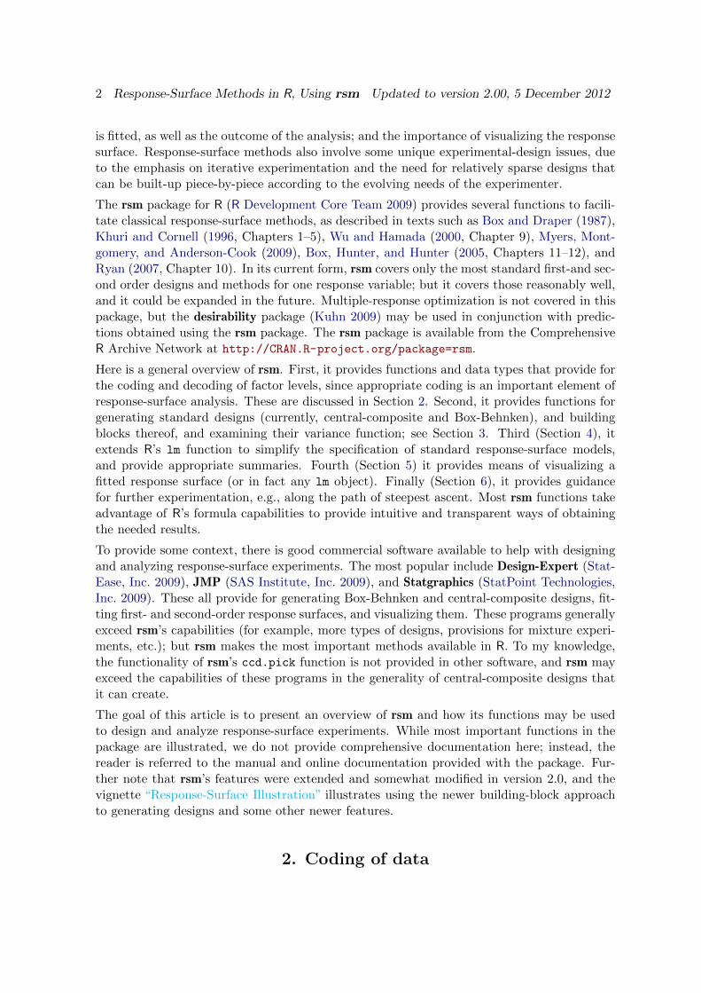
is fitted, as well as the outcome of the analysis; and the importance of visualizing the responsesurface. Response-surface methods also involve some unique experimental-design issues, dueto the emphasis on iterative experimentation and the need for relatively sparse designs thatcan be built-up piece-by-piece according to the evolving needs of the experimenter.
The rsm package for R (R Development Core Team 2009) provides several functions to facili-tate classical response-surface methods, as described in texts such as Box and Draper (1987),Khuri and Cornell (1996, Chapters 1–5), Wu and Hamada (2000, Chapter 9), Myers, Mont-gomery, and Anderson-Cook (2009), Box, Hunter, and Hunter (2005, Chapters 11–12), andRyan (2007, Chapter 10). In its current form, rsm covers only the most standard first-and sec-ond order designs and methods for one response variable; but it covers those reasonably well,and it could be expanded in the future. Multiple-response optimization is not covered in thispackage, but the desirability package (Kuhn 2009) may be used in conjunction with predic-tions obtained using the rsm package. The rsm package is available from the ComprehensiveR Archive Network at http://CRAN.R-project.org/package=rsm.
Here is a general overview of rsm. First, it provides functions and data types that provide forthe coding and decoding of factor levels, since appropriate coding is an important element ofresponse-surface analysis. These are discussed in Section 2. Second, it provides functions forgenerating standard designs (currently, central-composite and Box-Behnken), and buildingblocks thereof, and examining their variance function; see Section 3. Third (Section 4), itextends R’s lm function to simplify the specification of standard response-surface models,and provide appropriate summaries. Fourth (Section 5) it provides means of visualizing afitted response surface (or in fact any lm object). Finally (Section 6), it provides guidancefor further experimentation, e.g., along the path of steepest ascent. Most rsm functions takeadvantage of R’s formula capabilities to provide intuitive and transparent ways of obtainingthe needed results.
To provide some context, there is good commercial software available to help with designingand analyzing response-surface experiments. The most popular include Design-Expert (Stat-Ease, Inc. 2009), JMP (SAS Institute, Inc. 2009), and Statgraphics (StatPoint Technologies,Inc. 2009). These all provide for generating Box-Behnken and central-composite designs, fit-ting first- and second-order response surfaces, and visualizing them. These programs generallyexceed rsm’s capabilities (for example, more types of designs, provisions for mixture experi-ments, etc.); but rsm makes the most important methods available in R. To my knowledge,the functionality of rsm’s ccd.pick function is not provided in other software, and rsm mayexceed the capabilities of these programs in the generality of central-composite designs thatit can create.
The goal of this article is to present an overview of rsm and how its functions may be usedto design and analyze response-surface experiments. While most important functions in thepackage are illustrated, we do not provide comprehensive documentation here; instead, thereader is referred to the manual and online documentation provided with the package. Fur-ther note that rsm’s features were extended and somewhat modified in version 2.0, and thevignette “Response-Surface Illustration” illustrates using the newer building-block approachto generating designs and some other newer features.
2. Coding of data

Russell V. Lenth 3
An important aspect of response-surface analysis is using an appropriate coding transforma-tion of the data. The way the data are coded affects the results of canonical analysis (seeSection 4) and steepest-ascent analysis (see Section 6); for example, unless the scaling factorsare all equal, the path of steepest ascent obtained by fitting a model to the raw predictor val-ues will differ from the path obtained in the coded units, decoded to the original scale. Usinga coding method that makes all coded variables in the experiment vary over the same rangeis a way of giving each predictor an equal share in potentially determining the steepest-ascentpath. Thus, coding is an important step in response-surface analysis.
Accordingly, the rsm package provides for a coded.data class of objects, an extension ofdata.frame. The functions coded.data, as.coded.data, decode.data, recode.data, code2val,and val2code create or decode such objects. If a coded.data object is used in place of anordinary data.frame in the call to other rsm functions such as rsm (Section 4) or steepest
(Section 6), then appropriate additional output is provided that translates the results to theoriginal units. The print method for a coded.data object displays the coding formulas andthe data in either coded or decoded form.
As an example, consider the provided dataset ChemReact, which comes from Table 7.6 ofMyers et al. (2009).
> library("rsm")
> ChemReact
Time Temp Block Yield
1 80.00 170.00 B1 80.5
2 80.00 180.00 B1 81.5
3 90.00 170.00 B1 82.0
4 90.00 180.00 B1 83.5
5 85.00 175.00 B1 83.9
6 85.00 175.00 B1 84.3
7 85.00 175.00 B1 84.0
8 85.00 175.00 B2 79.7
9 85.00 175.00 B2 79.8
10 85.00 175.00 B2 79.5
11 92.07 175.00 B2 78.4
12 77.93 175.00 B2 75.6
13 85.00 182.07 B2 78.5
14 85.00 167.93 B2 77.0
In this experiment, the data in block B1 were collected first and analyzed, after which block B2
was added and a new analysis was done. The provided datasets ChemReact1 and ChemReact2
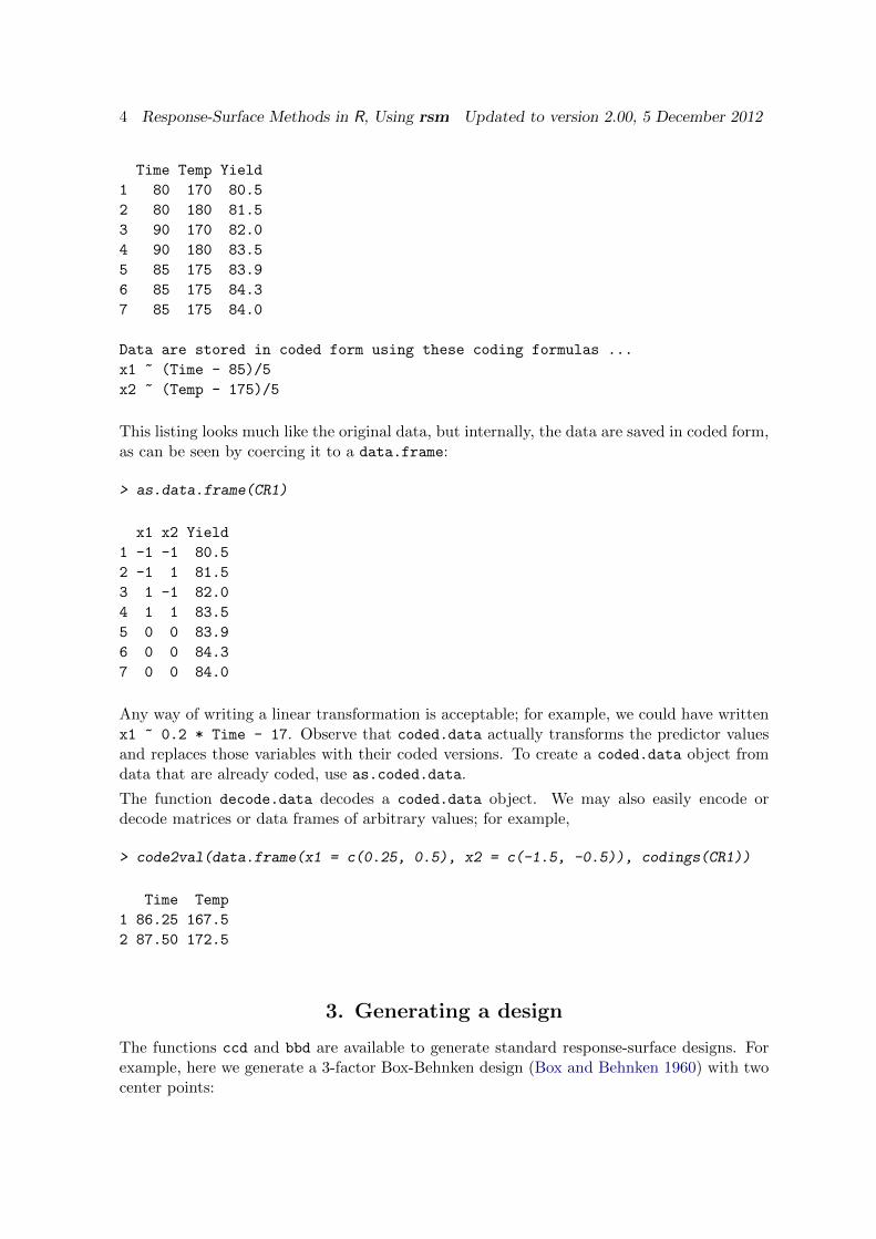
provide these separate blocks. The first block, ChemReact1, uses factor settings of Time =85 ± 5 and Temp = 175 ± 5, with three center points. Thus, the coded variables are x1 =(Time − 85)/5 and x1 = (Temp − 175)/5. To create a coded dataset with the appropriatecodings, provide this information via formulas:
> CR1 <- coded.data(ChemReact1, x1 ~ (Time - 85)/5, x2 ~ (Temp - 175)/5)
> CR1
4 Response-Surface Methods in R, Using rsm Updated to version 2.00, 5 December 2012
Time Temp Yield
1 80 170 80.5
2 80 180 81.5
3 90 170 82.0
4 90 180 83.5
5 85 175 83.9
6 85 175 84.3
7 85 175 84.0
Data are stored in coded form using these coding formulas ...
x1 ~ (Time - 85)/5
x2 ~ (Temp - 175)/5
This listing looks much like the original data, but internally, the data are saved in coded form,as can be seen by coercing it to a data.frame:
> as.data.frame(CR1)
x1 x2 Yield
1 -1 -1 80.5
2 -1 1 81.5
3 1 -1 82.0
4 1 1 83.5
5 0 0 83.9
6 0 0 84.3
7 0 0 84.0
Any way of writing a linear transformation is acceptable; for example, we could have writtenx1 ~ 0.2 * Time - 17. Observe that coded.data actually transforms the predictor valuesand replaces those variables with their coded versions. To create a coded.data object fromdata that are already coded, use as.coded.data.
The function decode.data decodes a coded.data object. We may also easily encode ordecode matrices or data frames of arbitrary values; for example,
> code2val(data.frame(x1 = c(0.25, 0.5), x2 = c(-1.5, -0.5)), codings(CR1))
Time Temp
1 86.25 167.5
2 87.50 172.5
3. Generating a design
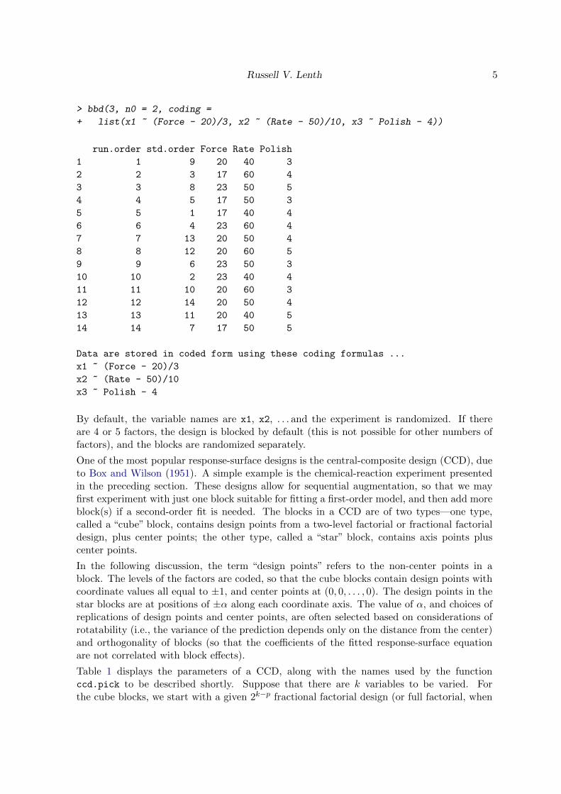
The functions ccd and bbd are available to generate standard response-surface designs. Forexample, here we generate a 3-factor Box-Behnken design (Box and Behnken 1960) with twocenter points:
Russell V. Lenth 5
> bbd(3, n0 = 2, coding =
+ list(x1 ~ (Force - 20)/3, x2 ~ (Rate - 50)/10, x3 ~ Polish - 4))
run.order std.order Force Rate Polish
1 1 9 20 40 3
2 2 3 17 60 4
3 3 8 23 50 5
4 4 5 17 50 3
5 5 1 17 40 4
6 6 4 23 60 4
7 7 13 20 50 4
8 8 12 20 60 5
9 9 6 23 50 3
10 10 2 23 40 4
11 11 10 20 60 3
12 12 14 20 50 4
13 13 11 20 40 5
14 14 7 17 50 5
Data are stored in coded form using these coding formulas ...
x1 ~ (Force - 20)/3
x2 ~ (Rate - 50)/10
x3 ~ Polish - 4
By default, the variable names are x1, x2, . . . and the experiment is randomized. If thereare 4 or 5 factors, the design is blocked by default (this is not possible for other numbers offactors), and the blocks are randomized separately.
One of the most popular response-surface designs is the central-composite design (CCD), dueto Box and Wilson (1951). A simple example is the chemical-reaction experiment presentedin the preceding section. These designs allow for sequential augmentation, so that we mayfirst experiment with just one block suitable for fitting a first-order model, and then add moreblock(s) if a second-order fit is needed. The blocks in a CCD are of two types—one type,called a “cube” block, contains design points from a two-level factorial or fractional factorialdesign, plus center points; the other type, called a “star” block, contains axis points pluscenter points.
In the following discussion, the term “design points” refers to the non-center points in ablock. The levels of the factors are coded, so that the cube blocks contain design points withcoordinate values all equal to ±1, and center points at (0, 0, . . . , 0). The design points in thestar blocks are at positions of ±α along each coordinate axis. The value of α, and choices ofreplications of design points and center points, are often selected based on considerations ofrotatability (i.e., the variance of the prediction depends only on the distance from the center)and orthogonality of blocks (so that the coefficients of the fitted response-surface equationare not correlated with block effects).
Table 1 displays the parameters of a CCD, along with the names used by the functionccd.pick to be described shortly. Suppose that there are k variables to be varied. Forthe cube blocks, we start with a given 2k−p fractional factorial design (or full factorial, when

6 Response-Surface Methods in R, Using rsm Updated to version 2.00, 5 December 2012
Parameter(s) Cube block(s) Star block(s)
Design points (±1,±1, . . . ,±1) (±α, 0, 0, . . . , 0), . . . , (0, 0, . . . ,±α)
Center points (0, 0, . . . , 0) (0, 0, . . . , 0)
# Distinct design points 2k−p (altogether) 2k
# Fractions of 2k−p blks.c (Not applicable)
Reps of each design point,within each block
wbr.c wbr.s
# Design pts each block n.c = wbr.cblks.c · 2
k−p n.s = wbr.s · (2k)
# Center points n0.c n0.s
# Points in each block n.c + n0.c n.s + n0.s
Reps of each block bbr.c bbr.s
Total observations (N)blks.c * bbr.c * (n.c + n0.c)
+ bbr.s * (n.s + n0.s)
Table 1: Parameters of a central-composite design, and names used by ccd.pick.
p = 0). We may either use this design as-is to define the design points in the cube block(s).Alternatively, we may confound one or more effects with blocks to split this design into blks.c
smaller cube blocks, in which case each cube block contains 2k−p/blks.c distinct design points.The star blocks always contain all 2k distinct design points—two on each axis.
Once the designs are decided, we may, if we like, replicate them within blocks. We may alsoreplicate the center points. The names wbr.c and wbr.s (for “within-block reps”) refer to thenumber of replicates of each design point within each cube block or star block, respectively.Thus, each cube block has a total of n.c = wbr.c · 2k−p/blks.c design points, and each starblock contains wbr.s · 2k design points. We may also replicate the center points—n0.c timesin each cube block, n0.s times within each star block.
Finally, we may replicate the blocks themselves; the numbers of such between-block replica-tions are denoted bbr.c and bbr.s for cube blocks and star blocks, respectively. It is im-portant to understand that each block is separately randomized, in effect a mini-experimentwithin the larger experiment. Having between-block replications means repeating these mini-experiments. We run an entire block before running another block.
The function ccd.pick is designed to help identify good CCDs. It simply creates a gridof all combinations of design choices, computes the α values required for orthogonality androtatability, sorts them by a specified criterion (by default, a measure of the discrepancybetween these two αs), and presents the best few.
For example, suppose that we want to experiment with k = 5 factors, and we are willingto consider CCDs with blks.c = 1, 2, or 4 cube blocks of sizes n.c = 8 or 16 each. Withthis many factors, the number of different star points (2k = 10) is relatively small comparedwith the size of some cube blocks (16), so it seems reasonable to consider either one or two
Russell V. Lenth 7
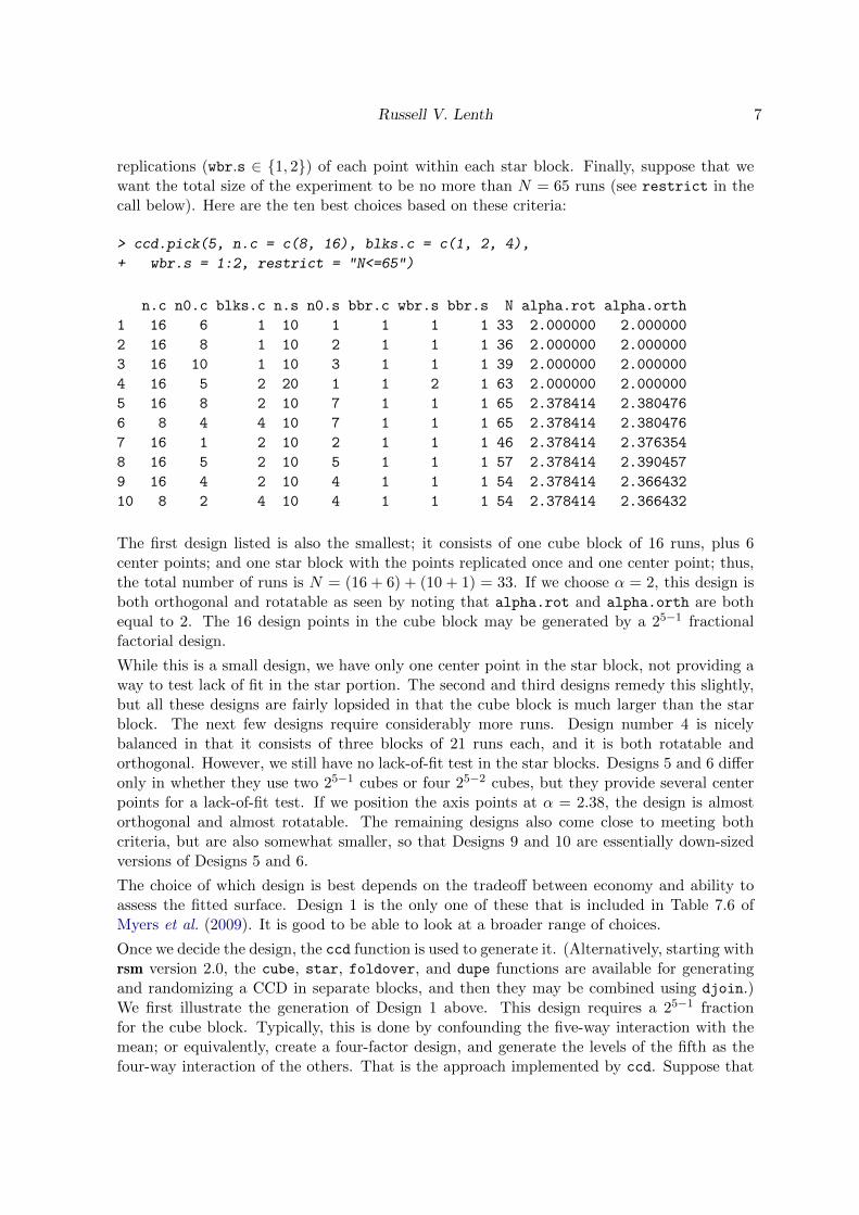
replications (wbr.s ∈ {1, 2}) of each point within each star block. Finally, suppose that wewant the total size of the experiment to be no more than N = 65 runs (see restrict in thecall below). Here are the ten best choices based on these criteria:
> ccd.pick(5, n.c = c(8, 16), blks.c = c(1, 2, 4),
+ wbr.s = 1:2, restrict = "N<=65")
n.c n0.c blks.c n.s n0.s bbr.c wbr.s bbr.s N alpha.rot alpha.orth
1 16 6 1 10 1 1 1 1 33 2.000000 2.000000
2 16 8 1 10 2 1 1 1 36 2.000000 2.000000
3 16 10 1 10 3 1 1 1 39 2.000000 2.000000
4 16 5 2 20 1 1 2 1 63 2.000000 2.000000
5 16 8 2 10 7 1 1 1 65 2.378414 2.380476
6 8 4 4 10 7 1 1 1 65 2.378414 2.380476
7 16 1 2 10 2 1 1 1 46 2.378414 2.376354
8 16 5 2 10 5 1 1 1 57 2.378414 2.390457
9 16 4 2 10 4 1 1 1 54 2.378414 2.366432
10 8 2 4 10 4 1 1 1 54 2.378414 2.366432
The first design listed is also the smallest; it consists of one cube block of 16 runs, plus 6center points; and one star block with the points replicated once and one center point; thus,the total number of runs is N = (16 + 6) + (10 + 1) = 33. If we choose α = 2, this design isboth orthogonal and rotatable as seen by noting that alpha.rot and alpha.orth are bothequal to 2. The 16 design points in the cube block may be generated by a 25−1 fractionalfactorial design.
While this is a small design, we have only one center point in the star block, not providing away to test lack of fit in the star portion. The second and third designs remedy this slightly,but all these designs are fairly lopsided in that the cube block is much larger than the starblock. The next few designs require considerably more runs. Design number 4 is nicelybalanced in that it consists of three blocks of 21 runs each, and it is both rotatable andorthogonal. However, we still have no lack-of-fit test in the star blocks. Designs 5 and 6 differonly in whether they use two 25−1 cubes or four 25−2 cubes, but they provide several centerpoints for a lack-of-fit test. If we position the axis points at α = 2.38, the design is almostorthogonal and almost rotatable. The remaining designs also come close to meeting bothcriteria, but are also somewhat smaller, so that Designs 9 and 10 are essentially down-sizedversions of Designs 5 and 6.
The choice of which design is best depends on the tradeoff between economy and ability toassess the fitted surface. Design 1 is the only one of these that is included in Table 7.6 ofMyers et al. (2009). It is good to be able to look at a broader range of choices.
Once we decide the design, the ccd function is used to generate it. (Alternatively, starting withrsm version 2.0, the cube, star, foldover, and dupe functions are available for generatingand randomizing a CCD in separate blocks, and then they may be combined using djoin.)We first illustrate the generation of Design 1 above. This design requires a 25−1 fractionfor the cube block. Typically, this is done by confounding the five-way interaction with themean; or equivalently, create a four-factor design, and generate the levels of the fifth as thefour-way interaction of the others. That is the approach implemented by ccd. Suppose that
8 Response-Surface Methods in R, Using rsm Updated to version 2.00, 5 December 2012
we denote the design factors by A,B,C,D,E; let’s opt to use E = −ABCD as the generator.The following call generates the design (results not shown):
> des1 <- ccd (y1 + y2 ~ A + B + C + D,
+ generators = E ~ - A * B * C * D, n0 = c(6, 1))
The value of α was not specified, and by default it uses the α for orthogonality. The firstargument could have been just 4, but then the generator would have had to have been givenin terms of the default variable names x1, x2, . . . . The optional left-hand side in the formulacreates place-holders for response variable(s), to be filled-in with data later. As in bbd, wecould have added coding formulas to create a coded.data object.
Next, we illustrate the generation of Design 10. This design has four 25−2 cube blocks with2 center points each, and one unreplicated star block with 4 center points. The non-centerpoints in the cube blocks comprise 4× 8 = 32 runs, so we most likely want to create them bydividing the full 25 factorial into four fractional blocks. We can for example opt to generatethe blocks via the factors b1 = ABC and b2 = CDE, so that the blocks are determinedby the four combinations of b1 and b2. Then the block effects will be confounded with theeffects ABC, CDE, and also the b1b2 interaction ABC2DE = ABDE. It is important inresponse-surface work to avoid confounding second-order interactions, and this scheme is thusacceptable. Unlike Design 1, this design includes all 25 factor combinations, so we do not usethe generators argument; instead, we use blocks to do the fractionation:
> des10 <- ccd( ~ A + B + C + D + E,
+ blocks = Blk ~ c(A * B * C, C * D * E), n0 = c(2, 4))
Each block is randomized separately, but the order of the blocks is not randomized. Inpractice, we may opt to run the blocks in a different sequence. With this design, just one ofthe cube blocks is sufficient to estimate a first-order response surface.
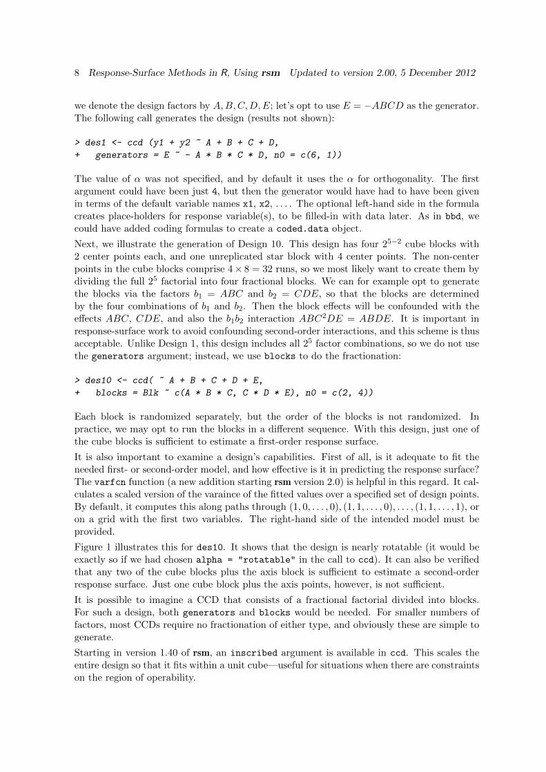
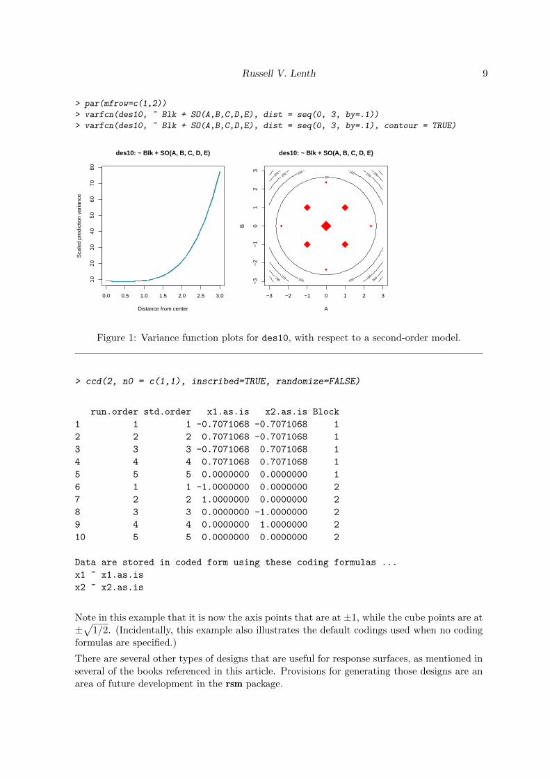
It is also important to examine a design’s capabilities. First of all, is it adequate to fit theneeded first- or second-order model, and how effective is it in predicting the response surface?The varfcn function (a new addition starting rsm version 2.0) is helpful in this regard. It cal-culates a scaled version of the varaince of the fitted values over a specified set of design points.By default, it computes this along paths through (1, 0, . . . , 0), (1, 1, . . . , 0), . . . , (1, 1, . . . , 1), oron a grid with the first two variables. The right-hand side of the intended model must beprovided.
Figure 1 illustrates this for des10. It shows that the design is nearly rotatable (it would beexactly so if we had chosen alpha = "rotatable" in the call to ccd). It can also be verifiedthat any two of the cube blocks plus the axis block is sufficient to estimate a second-orderresponse surface. Just one cube block plus the axis points, however, is not sufficient.
It is possible to imagine a CCD that consists of a fractional factorial divided into blocks.For such a design, both generators and blocks would be needed. For smaller numbers offactors, most CCDs require no fractionation of either type, and obviously these are simple togenerate.
Starting in version 1.40 of rsm, an inscribed argument is available in ccd. This scales theentire design so that it fits within a unit cube—useful for situations when there are constraintson the region of operability.
Russell V. Lenth 9
> par(mfrow=c(1,2))
> varfcn(des10, ~ Blk + SO(A,B,C,D,E), dist = seq(0, 3, by=.1))
> varfcn(des10, ~ Blk + SO(A,B,C,D,E), dist = seq(0, 3, by=.1), contour = TRUE)
0.0 0.5 1.0 1.5 2.0 2.5 3.0
1020
3040
5060
7080
des10: ~ Blk + SO(A, B, C, D, E)
Distance from center
Sca
led
pred
ictio
n va
rianc
e
des10: ~ Blk + SO(A, B, C, D, E)
A
B
50
100
100
100
100
150
150
150
150
200
200
200
200
−3 −2 −1 0 1 2 3
−3
−2
−1
01
23
Figure 1: Variance function plots for des10, with respect to a second-order model.
> ccd(2, n0 = c(1,1), inscribed=TRUE, randomize=FALSE)
run.order std.order x1.as.is x2.as.is Block
1 1 1 -0.7071068 -0.7071068 1
2 2 2 0.7071068 -0.7071068 1
3 3 3 -0.7071068 0.7071068 1
4 4 4 0.7071068 0.7071068 1
5 5 5 0.0000000 0.0000000 1
6 1 1 -1.0000000 0.0000000 2
7 2 2 1.0000000 0.0000000 2
8 3 3 0.0000000 -1.0000000 2
9 4 4 0.0000000 1.0000000 2
10 5 5 0.0000000 0.0000000 2
Data are stored in coded form using these coding formulas ...
x1 ~ x1.as.is
x2 ~ x2.as.is
Note in this example that it is now the axis points that are at ±1, while the cube points are at±√
1/2. (Incidentally, this example also illustrates the default codings used when no codingformulas are specified.)
There are several other types of designs that are useful for response surfaces, as mentioned inseveral of the books referenced in this article. Provisions for generating those designs are anarea of future development in the rsm package.

10 Response-Surface Methods in R, Using rsm Updated to version 2.00, 5 December 2012
4. Fitting a response-surface model
A response surface is fitted using the rsm function. This is an extension of lm, and worksalmost exactly like it; however, the model formula for rsm must make use of the specialfunctions FO, TWI, PQ, or SO (for “first-order,”, “two-way interaction,” “pure quadratic,” and“second-order,” respectively), because the presence of these specifies the response-surface por-tion of the model. Other terms that don’t involve these functions may be included in themodel; often, these terms would include blocking factors and other categorical predictors.
To illustrate this, let us revisit the ChemReact data introduced in Section 2. We have oneresponse variable, Yield, and two coded predictors x1 and x2 as well as a blocking factorBlock. Supposing that the experiment was done in two stages, we first act as though the datain the second block have not yet been collected; and fit a first-order response-surface modelto the data in the first block:
> CR1.rsm <- rsm(Yield ~ FO(x1, x2), data = CR1)
> summary(CR1.rsm)
Call:
rsm(formula = Yield ~ FO(x1, x2), data = CR1)
Estimate Std. Error t value Pr(>|t|)
(Intercept) 82.81429 0.54719 151.3456 1.143e-08 ***
x1 0.87500 0.72386 1.2088 0.2933
x2 0.62500 0.72386 0.8634 0.4366
---
Signif. codes: 0 '***' 0.001 '**' 0.01 '*' 0.05 '.' 0.1 ' ' 1
Multiple R-squared: 0.3555, Adjusted R-squared: 0.0333
F-statistic: 1.103 on 2 and 4 DF, p-value: 0.4153
Analysis of Variance Table
Response: Yield
Df Sum Sq Mean Sq F value Pr(>F)
FO(x1, x2) 2 4.6250 2.3125 1.1033 0.41534
Residuals 4 8.3836 2.0959
Lack of fit 2 8.2969 4.1485 95.7335 0.01034
Pure error 2 0.0867 0.0433
Direction of steepest ascent (at radius 1):
x1 x2
0.8137335 0.5812382
Corresponding increment in original units:
Time Temp
4.068667 2.906191
What we see in the summary is the usual summary for a lm object (with a subtle difference),
Russell V. Lenth 11
followed by some additional information particular to response surfaces. The subtle differenceis that the labeling of the regression coefficients is simplified (we don’t see “FO” in there). Theanalysis-of-variance table shown includes a breakdown of lack of fit and pure error, and weare also given information about the direction of steepest ascent. Since the dataset is acoded.data object, the steepest-ascent information is also presented in original units. (Whilersm does not require a coded.data dataset, the use of one is highly recommended.)
In this particular example, the steepest-ascent information is of little use, because there issignificant lack of fit for this model (p ≈ 0.01). It suggests that we should try a higher-ordermodel. For example, we could add two-way interactions:
> CR1.rsmi <- update(CR1.rsm, . ~ . + TWI(x1, x2))
> summary(CR1.rsmi)
The results are not shown, but one finds there is still a small p value for lack-of-fit.
To go further, we need more data. Thus, let us pretend that we now collect the data in thesecond block. Then here are the data from the combined blocks:
> ( CR2 <- djoin(CR1, ChemReact2) )
Time Temp Yield Block
1 80.00 170.00 80.5 1
2 80.00 180.00 81.5 1
3 90.00 170.00 82.0 1
4 90.00 180.00 83.5 1
5 85.00 175.00 83.9 1
6 85.00 175.00 84.3 1
7 85.00 175.00 84.0 1
8 85.00 175.00 79.7 2
9 85.00 175.00 79.8 2
10 85.00 175.00 79.5 2
11 92.07 175.00 78.4 2
12 77.93 175.00 75.6 2
13 85.00 182.07 78.5 2
14 85.00 167.93 77.0 2
Data are stored in coded form using these coding formulas ...
x1 ~ (Time - 85)/5
x2 ~ (Temp - 175)/5
Notice that djoin figures out the fact that ChemReact2 is not coded but it has the appropriateuncoded variables Time and Temp; so it codes those variables appropriately. Also, the Block
factor is added automatically.
We are now in the position of fitting a full second-order model to the combined data. Thiscan be done by adding PQ(x1, x2) to the above model with interaction, but the easier wayis to use SO, which is shorthand for a model with FO, TWI, and PQ terms. Also, we now needto account for the block effect since the data are collected in separate experiments:

12 Response-Surface Methods in R, Using rsm Updated to version 2.00, 5 December 2012
> CR2.rsm <- rsm(Yield ~ Block + SO(x1, x2), data = CR2)
> summary(CR2.rsm)
Call:
rsm(formula = Yield ~ Block + SO(x1, x2), data = CR2)
Estimate Std. Error t value Pr(>|t|)
(Intercept) 84.095427 0.079631 1056.067 < 2.2e-16 ***
Block2 -4.457530 0.087226 -51.103 2.877e-10 ***
x1 0.932541 0.057699 16.162 8.444e-07 ***
x2 0.577712 0.057699 10.012 2.122e-05 ***
x1:x2 0.125000 0.081592 1.532 0.1694
x1^2 -1.308555 0.060064 -21.786 1.083e-07 ***
x2^2 -0.933442 0.060064 -15.541 1.104e-06 ***
---
Signif. codes: 0 '***' 0.001 '**' 0.01 '*' 0.05 '.' 0.1 ' ' 1
Multiple R-squared: 0.9981, Adjusted R-squared: 0.9964
F-statistic: 607.2 on 6 and 7 DF, p-value: 3.811e-09
Analysis of Variance Table
Response: Yield
Df Sum Sq Mean Sq F value Pr(>F)
Block 1 69.531 69.531 2611.0950 2.879e-10
FO(x1, x2) 2 9.626 4.813 180.7341 9.450e-07
TWI(x1, x2) 1 0.063 0.063 2.3470 0.1694
PQ(x1, x2) 2 17.791 8.896 334.0539 1.135e-07
Residuals 7 0.186 0.027
Lack of fit 3 0.053 0.018 0.5307 0.6851
Pure error 4 0.133 0.033
Stationary point of response surface:
x1 x2
0.3722954 0.3343802
Stationary point in original units:
Time Temp
86.86148 176.67190
Eigenanalysis:
eigen() decomposition
$values
[1] -0.9233027 -1.3186949
$vectors
[,1] [,2]

Russell V. Lenth 13
x1 -0.1601375 -0.9870947
x2 -0.9870947 0.1601375
The lack of fit is now non-significant (p ≈ 0.69). The summary for a second-order modelprovides results of a canonical analysis of the surface rather than for steepest ascent. Theanalysis indicates that the stationary point of the fitted surface is at (0.37, 0.33) in codedunits—well within the experimental region; and that both eigenvalues are negative, indicatingthat the stationary point is a maximum. This is the kind of situation we dream for inresponse-surface experimentation—clear evidence of a nearby set of optimal conditions. Weshould probably collect some confirmatory data near this estimated optimum at Time ≈ 87,Temp ≈ 177, to make sure.
Another example that comes out a different way is a paper-helicopter experiment (Box et al.2005, Table 12.5). This is another central-composite experiment, in four variables and twoblocks. The data are provided in the rsm dataset heli; these data are already coded. Theoriginal variables are wing area A, wing shape R, body width W, and body length L. The goalis to make a paper helicopter that flies for as long as possible. Each observation in the datasetrepresents the results of ten replicated flights at each experimental condition. Here we studythe average flight time, variable name ave, using a second-order surface.
> heli.rsm <- rsm(ave ~ block + SO(x1, x2, x3, x4), data = heli)
> summary(heli.rsm)
Call:
rsm(formula = ave ~ block + SO(x1, x2, x3, x4), data = heli)
Estimate Std. Error t value Pr(>|t|)
(Intercept) 372.800000 1.506375 247.4815 < 2.2e-16 ***
block2 -2.950000 1.207787 -2.4425 0.0284522 *
x1 -0.083333 0.636560 -0.1309 0.8977075
x2 5.083333 0.636560 7.9856 1.398e-06 ***
x3 0.250000 0.636560 0.3927 0.7004292
x4 -6.083333 0.636560 -9.5566 1.633e-07 ***
x1:x2 -2.875000 0.779623 -3.6877 0.0024360 **
x1:x3 -3.750000 0.779623 -4.8100 0.0002773 ***
x1:x4 4.375000 0.779623 5.6117 6.412e-05 ***
x2:x3 4.625000 0.779623 5.9324 3.657e-05 ***
x2:x4 -1.500000 0.779623 -1.9240 0.0749257 .
x3:x4 -2.125000 0.779623 -2.7257 0.0164099 *
x1^2 -2.037500 0.603894 -3.3739 0.0045424 **
x2^2 -1.662500 0.603894 -2.7530 0.0155541 *
x3^2 -2.537500 0.603894 -4.2019 0.0008873 ***
x4^2 -0.162500 0.603894 -0.2691 0.7917877
---
Signif. codes: 0 '***' 0.001 '**' 0.01 '*' 0.05 '.' 0.1 ' ' 1
Multiple R-squared: 0.9555, Adjusted R-squared: 0.9078
F-statistic: 20.04 on 15 and 14 DF, p-value: 6.54e-07
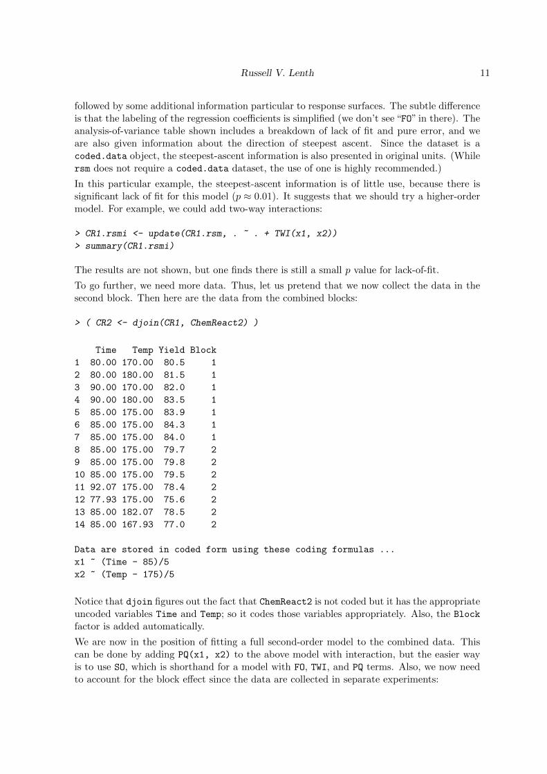
14 Response-Surface Methods in R, Using rsm Updated to version 2.00, 5 December 2012
Analysis of Variance Table
Response: ave
Df Sum Sq Mean Sq F value Pr(>F)
block 1 16.81 16.81 1.7281 0.209786
FO(x1, x2, x3, x4) 4 1510.00 377.50 38.8175 1.965e-07
TWI(x1, x2, x3, x4) 6 1114.00 185.67 19.0917 5.355e-06
PQ(x1, x2, x3, x4) 4 282.54 70.64 7.2634 0.002201
Residuals 14 136.15 9.72
Lack of fit 10 125.40 12.54 4.6660 0.075500
Pure error 4 10.75 2.69
Stationary point of response surface:
x1 x2 x3 x4
0.8607107 -0.3307115 -0.8394866 -0.1161465
Stationary point in original units:
A R W L
12.916426 2.434015 1.040128 1.941927
Eigenanalysis:
eigen() decomposition
$values
[1] 3.258222 -1.198324 -3.807935 -4.651963
$vectors
[,1] [,2] [,3] [,4]
x1 0.5177048 0.04099358 0.7608371 -0.38913772
x2 -0.4504231 0.58176202 0.5056034 0.45059647
x3 -0.4517232 0.37582195 -0.1219894 -0.79988915
x4 0.5701289 0.72015994 -0.3880860 0.07557783
From the analysis of variance, it is clear that the second-order (TWI and PQ) terms contributesignificantly to the model, so the canonical analysis is relevant. Again, the stationary point isfairly near the experimental region, but the eigenvalues are of mixed sign, indicating that itis a saddle point (neither a maximum nor a minimum). We will do further analysis of theseresults in subsequent sections.
5. Displaying a response surface
While the canonical analysis gives us a handle on the behavior of a second-order responsesurface, an effective graph is a lot easier to present and explain. To that end, rsm includes afunction for making contour plots of a fitted response surface. This function is not restrictedto rsm results, however; it can be used for plotting any regression surface produced by lm.For more detailed information, see the associated vignette “Surface Plots in the rsm Package.”

Russell V. Lenth 15
11.5 12.0 12.5 13.0 13.5
2.0
2.2
2.4
2.6
2.8
3.0
ASlice at W = 1.04, L = 1.94, x1 = 0.860710709095187, x2 = −0.330711524873929
R
345
355 360
360
365
365
370
11.5 12.0 12.5 13.0 13.50.
81.
01.
21.
41.
6
ASlice at R = 2.43, L = 1.94, x1 = 0.860710709095187, x3 = −0.839486624210177
W
345
350
355
355
360
360
365
365
370
11.5 12.0 12.5 13.0 13.5
1.0
1.5
2.0
2.5
3.0
ASlice at R = 2.43, W = 1.04, x1 = 0.860710709095187, x4 = −0.116146514721039
L
335
3
45
350
355
360
365
365
370
370
375
375
2.0 2.2 2.4 2.6 2.8 3.0
0.8
1.0
1.2
1.4
1.6
RSlice at A = 12.92, L = 1.94, x2 = −0.330711524873929, x3 = −0.839486624210177
W
335
345 350
355
355
360
360
365
365
370
370
2.0 2.2 2.4 2.6 2.8 3.0
1.0
1.5
2.0
2.5
3.0
RSlice at A = 12.92, W = 1.04, x2 = −0.330711524873929, x4 = −0.116146514721039
L
360
365
365
370
370
0.8 1.0 1.2 1.4 1.6
1.0
1.5
2.0
2.5
3.0
WSlice at A = 12.92, R = 2.43, x3 = −0.839486624210177, x4 = −0.116146514721039
L
345 350
355 360
365 365
370
370
Figure 2: Fitted response-surface contour plots near the stationary point for the helicopterexperiment.
We provide the lm or rsm object, a formula for which predictors to use, and various optionalparameters. Consider the paper-helicopter example in the preceding section; there are fourresponse-surface predictors, making six pairs of predictors. If we want to visualize the behaviorof the fitted surface around the stationary point, we can provide that location as the at
argument:
> par(mfrow = c(2, 3))
> contour(heli.rsm, ~ x1 + x2 + x3 + x4, image = TRUE,
+ at = summary(heli.rsm)$canonical$xs)
The plots are shown in Figure 2. The image argument causes each plot to display a colorimage overlaid by the contour lines. When multiple plots like this are produced, the colorlevels are held consistent across all plots. Note that the at condition does not set the centerof the coordinate systems (the default variable ranges are derived from the data); it sets thevalues at which to hold variables other than those on one of the coordinate axes, as shown inthe subtitles.
6. Direction for further experimentation
In many first-order cases, as well as second-order cases where we find a saddle point or thestationary point is distant, the most useful further action is to decide in which direction toexplore further. In the case of first-order models, one can follow the direction of steepestascent. As already seen in Section 4, the summary method for rsm objects provides some
16 Response-Surface Methods in R, Using rsm Updated to version 2.00, 5 December 2012
information about this path. More detailed information is available via the steepest function;for example,
> steepest(CR1.rsm, dist = c(0, 0.5, 1))
Path of steepest ascent from ridge analysis:
dist x1 x2 | Time Temp | yhat
1 0.0 0.000 0.000 | 85.000 175.000 | 82.814
2 0.5 0.407 0.291 | 87.035 176.455 | 83.352
3 1.0 0.814 0.581 | 89.070 177.905 | 83.890
In general, we can specify any set of distances along the path. The decoded coordinate valuesare displayed if the model was fitted to a coded.data dataset.
At this point it is worth emphasizing that, although the fitted values are also displayed,one must be careful to understand that these are only predictions and that, as the distanceincreases, they are very poor predictions and should be taken with a grain of salt. Whatone should do is to conduct actual experimental runs at points along this path, and use theobserved response values, not these predictions, for guidance on where to locate the nextfactorial experiment.
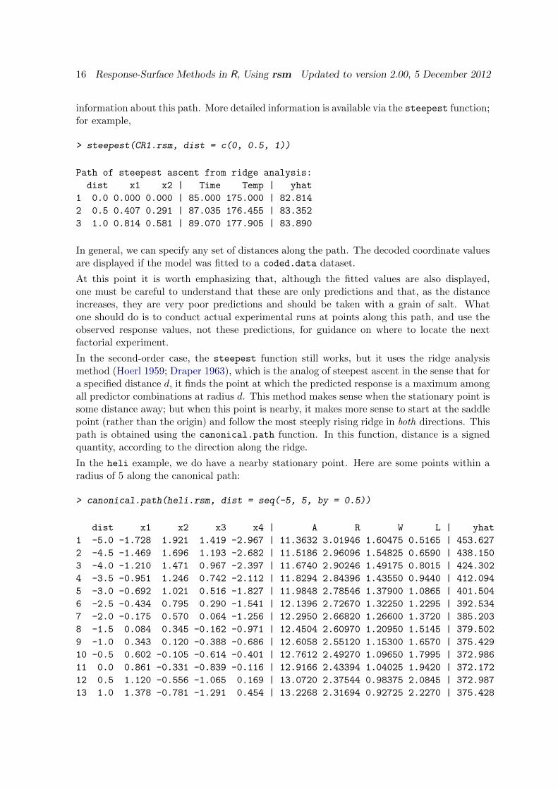
In the second-order case, the steepest function still works, but it uses the ridge analysismethod (Hoerl 1959; Draper 1963), which is the analog of steepest ascent in the sense that fora specified distance d, it finds the point at which the predicted response is a maximum amongall predictor combinations at radius d. This method makes sense when the stationary point issome distance away; but when this point is nearby, it makes more sense to start at the saddlepoint (rather than the origin) and follow the most steeply rising ridge in both directions. Thispath is obtained using the canonical.path function. In this function, distance is a signedquantity, according to the direction along the ridge.
In the heli example, we do have a nearby stationary point. Here are some points within aradius of 5 along the canonical path:
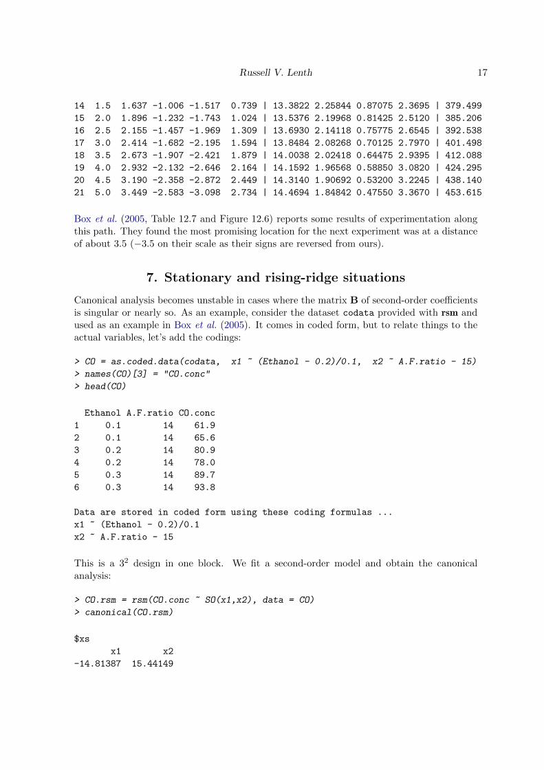
> canonical.path(heli.rsm, dist = seq(-5, 5, by = 0.5))
dist x1 x2 x3 x4 | A R W L | yhat
1 -5.0 -1.728 1.921 1.419 -2.967 | 11.3632 3.01946 1.60475 0.5165 | 453.627
2 -4.5 -1.469 1.696 1.193 -2.682 | 11.5186 2.96096 1.54825 0.6590 | 438.150
3 -4.0 -1.210 1.471 0.967 -2.397 | 11.6740 2.90246 1.49175 0.8015 | 424.302
4 -3.5 -0.951 1.246 0.742 -2.112 | 11.8294 2.84396 1.43550 0.9440 | 412.094
5 -3.0 -0.692 1.021 0.516 -1.827 | 11.9848 2.78546 1.37900 1.0865 | 401.504
6 -2.5 -0.434 0.795 0.290 -1.541 | 12.1396 2.72670 1.32250 1.2295 | 392.534
7 -2.0 -0.175 0.570 0.064 -1.256 | 12.2950 2.66820 1.26600 1.3720 | 385.203
8 -1.5 0.084 0.345 -0.162 -0.971 | 12.4504 2.60970 1.20950 1.5145 | 379.502
9 -1.0 0.343 0.120 -0.388 -0.686 | 12.6058 2.55120 1.15300 1.6570 | 375.429
10 -0.5 0.602 -0.105 -0.614 -0.401 | 12.7612 2.49270 1.09650 1.7995 | 372.986
11 0.0 0.861 -0.331 -0.839 -0.116 | 12.9166 2.43394 1.04025 1.9420 | 372.172
12 0.5 1.120 -0.556 -1.065 0.169 | 13.0720 2.37544 0.98375 2.0845 | 372.987
13 1.0 1.378 -0.781 -1.291 0.454 | 13.2268 2.31694 0.92725 2.2270 | 375.428
Russell V. Lenth 17
14 1.5 1.637 -1.006 -1.517 0.739 | 13.3822 2.25844 0.87075 2.3695 | 379.499
15 2.0 1.896 -1.232 -1.743 1.024 | 13.5376 2.19968 0.81425 2.5120 | 385.206
16 2.5 2.155 -1.457 -1.969 1.309 | 13.6930 2.14118 0.75775 2.6545 | 392.538
17 3.0 2.414 -1.682 -2.195 1.594 | 13.8484 2.08268 0.70125 2.7970 | 401.498
18 3.5 2.673 -1.907 -2.421 1.879 | 14.0038 2.02418 0.64475 2.9395 | 412.088
19 4.0 2.932 -2.132 -2.646 2.164 | 14.1592 1.96568 0.58850 3.0820 | 424.295
20 4.5 3.190 -2.358 -2.872 2.449 | 14.3140 1.90692 0.53200 3.2245 | 438.140
21 5.0 3.449 -2.583 -3.098 2.734 | 14.4694 1.84842 0.47550 3.3670 | 453.615
Box et al. (2005, Table 12.7 and Figure 12.6) reports some results of experimentation alongthis path. They found the most promising location for the next experiment was at a distanceof about 3.5 (−3.5 on their scale as their signs are reversed from ours).
7. Stationary and rising-ridge situations
Canonical analysis becomes unstable in cases where the matrix B of second-order coefficientsis singular or nearly so. As an example, consider the dataset codata provided with rsm andused as an example in Box et al. (2005). It comes in coded form, but to relate things to theactual variables, let’s add the codings:
> CO = as.coded.data(codata, x1 ~ (Ethanol - 0.2)/0.1, x2 ~ A.F.ratio - 15)
> names(CO)[3] = "CO.conc"
> head(CO)
Ethanol A.F.ratio CO.conc
1 0.1 14 61.9
2 0.1 14 65.6
3 0.2 14 80.9
4 0.2 14 78.0
5 0.3 14 89.7
6 0.3 14 93.8
Data are stored in coded form using these coding formulas ...
x1 ~ (Ethanol - 0.2)/0.1
x2 ~ A.F.ratio - 15
This is a 32 design in one block. We fit a second-order model and obtain the canonicalanalysis:
> CO.rsm = rsm(CO.conc ~ SO(x1,x2), data = CO)
> canonical(CO.rsm)
$xs
x1 x2
-14.81387 15.44149
18 Response-Surface Methods in R, Using rsm Updated to version 2.00, 5 December 2012
x1 = (Ethanol − 0.2)/0.1
x2 =
A.F
.rat
io −
15
−80
−80
−80
−80
−80
−80
−60
−60
−40
−40
−20
−20
0
20
40
60
80
−15 −10 −5 0
05
1015
●●
●●
●●
●●
●●
●●
●●
●●
●●
●●
●●
●●
●●
●●
●●
●●
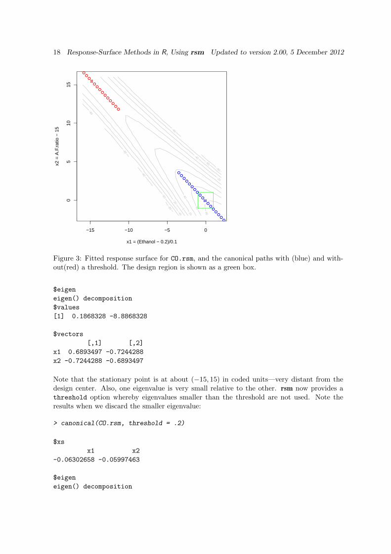
Figure 3: Fitted response surface for CO.rsm, and the canonical paths with (blue) and with-out(red) a threshold. The design region is shown as a green box.
$eigen
eigen() decomposition
$values
[1] 0.1868328 -8.8868328
$vectors
[,1] [,2]
x1 0.6893497 -0.7244288
x2 -0.7244288 -0.6893497
Note that the stationary point is at about (−15, 15) in coded units—very distant from thedesign center. Also, one eigenvalue is very small relative to the other. rsm now provides athreshold option whereby eigenvalues smaller than the threshold are not used. Note theresults when we discard the smaller eigenvalue:
> canonical(CO.rsm, threshold = .2)
$xs
x1 x2
-0.06302658 -0.05997463
$eigen
eigen() decomposition
Russell V. Lenth 19
$values
[1] 0.000000 -8.886833
$vectors
[,1] [,2]
x1 0.6893497 -0.7244288
x2 -0.7244288 -0.6893497
This sets the smaller eigenvalue to zero. By ignoring it, the stationary point is (−.06,−.06)—much, much closer to the design center.
The following statements produce an illustrative plot, shown in Figure 3.
> contour(CO.rsm, x2 ~ x1, bounds = list(x1=c(-16,2), x2=c(-2,16)),
+ zlim=c(-100,100), col="gray", decode = FALSE)
> lines(c(-1,1,1,-1,-1), c(-1,-1,1,1,-1), col="green") # design region
> points(x2 ~ x1, data=canonical.path(CO.rsm), col="red", pch=1+6*(dist==0))
> points(x2 ~ x1, data=canonical.path(CO.rsm, threshold=.2),
+ col="blue", pch=1+6*(dist==0))
It displays the fitted response surface, as well as the results from canonical.path with andwithout the threshold (blue and red points, respectively). The region of the design is shownas a green box. The stationary point (different symbol) is seen to be a saddle point nearthe upper-left corner when not thresholded, and near the design center whern thresholded.Otherwise, the canonical paths are much the same but with different origins. Both form apath along the rising ridge that occurs in the vicinity of the design.
It is important to note that the stationary point obtained by thresholding is not really astationary point, but rather a nearby point that represents a center for the most importantcanonical directions. In this example, the true stationary point is very distant, and thethresholded stationary point is the nearest place on a rising ridge that emanates from thetrue stationary point. The thresholded canonical.path results give us a much more usableset of factor settings to explore than the ones without a threshold.
The rest of this section provides some technical backing, in case you’re interested. Let b andB denote the first and second-order coefficients of the fitted second-order surface, so that thefitted value at a coded point x is y(x) = b0 +b′x+ x′Bx. The stationary point xs solves theequation 2Bxs + b = 0, i.e., xs = −1
2B−1b. The canonical analysis yields the decomposition
B = UΛΛΛU′ = λ1u1u′1 + λ2u2u
′2 + · · ·+ λkuku
′k
where there are k predictors, the uj form orthonormal columns of U, and the λj are theeigenvalues, and ΛΛΛ = diag(λ1, λ2, . . . , λk). It also happens to be true that
B−1 = UΛΛΛ−1U′ = 1λ1u1u
′1 + 1
λ2u2u
′2 + · · ·+ 1
λkuku
′k
Thus, a really small value of λj hardly affects B, but has a huge influence on B−1.
Now, for some m < k, let ΛΛΛ∗ be the m × m diagonal matrix with only some subset of meigenvalues; and let U∗ be the k ×m matrix with the corresponding uj . If we excluded thesmallest absolute eigenvalues, then B∗ = U∗ΛΛΛ∗U
′∗ ≈ B. Moreover, by orthogonality, U′B =

20 Response-Surface Methods in R, Using rsm Updated to version 2.00, 5 December 2012
ΛΛΛU′ and U′∗B = ΛΛΛ∗U′∗. The stationary point satisfies 2Bx+b = 0 so that 2U′∗Bx+U′∗b = 0.
Accordingly, we propose to define a pseudo-stationary point x∗ such that 2U′∗Bx∗+U′∗b = 0;i.e., 2ΛΛΛ∗U
′∗x∗ + U′∗b = 0.
This comprises m equations in k > m unknowns. To make it unique, we opt to choose thesolution that is closest to the origin; that is, minimize x′x subject to the constraint that2ΛΛΛ∗U
′∗x + U′∗b = 0. Using variational methods (Lagrange multipliers), we find that the
resulting solution is x∗ = −12U∗ΛΛΛ
−1∗ U′∗b. In other words, we simply exclude some terms
corresponding to small λi in the above expression for B−1. This is the stationary pointreturned in rsm’s canonical and related functions when a threshold is used to exclude somesmall eigenvalues.
8. Discussion
The current version of rsm provides only the most standard tools for first- and second-orderresponse-surface design and analysis. The package can be quite useful for those standardsituations, and it implements many of the analyses presented in textbooks. However, clearlya great deal of work has been done in response-surface methods that is not represented here.Even a quick glance at a review article such as Myers, Montgomery, Vining, Borror, andKowalski (2004)—or even an older one such as Hill and Hunter (1989)—reveals that there is agreat deal that could be added to future editions of rsm. There are many other useful designsbesides central composites and Box-Behnken designs. We can consider higher-order modelsor the use of predictor transformations. Mixture designs are not yet provided for. Thereare important relationships between these methods and robust parameter design, and withcomputer experiments. The list goes on. However, we now at least have a good collection ofbasic tools for the R platform, and that is a starting point.
References
Box GEP, Behnken DW (1960). “Some New Three Level Designs for the Study of QuantitativeVariables.” Technometrics, 2, 455–475.
Box GEP, Draper NR (1987). Empirical Model-Building and Response Surfaces. John Wiley& Sons, New York.
Box GEP, Hunter WG, Hunter JS (2005). Statistics for Experimenters: An Introduction toDesign, Data Analysis, and Model Building. 2nd edition. John Wiley & Sons, New York.
Box GEP, Wilson KB (1951). “On the Experimental Attainment of Optimum Conditions.”Journal of the Royal Statistical Society B, 13, 1–45.
Draper NR (1963). “‘Ridge Analysis’ of Response Surfaces.” Technometrics, 5, 469–479.
Hill WJ, Hunter WG (1989). “A Review of Response Surface Methodology: A LiteratureReview.” Technometrics, 8, 571–590.
Hoerl AE (1959). “Optimum Solution of Many Variables Equations.” Chemical EngineeringProgress, 55, 67–78.

Russell V. Lenth 21
Khuri AI, Cornell JA (1996). Responses Surfaces: Design and Analyses. 2nd edition. MarcelDekker, Monticello, NY.
Kuhn M (2009). desirability: Desirability Function Optimization and Ranking. R packageversion 1.02, URL http://CRAN.R-project.org/package=desirability.
Lenth RV (2009). “Response-Surface Methods in R, Using rsm.” Journal of Statistical Soft-ware, 32(7), 1–17. URL http://www.jstatsoft.org/v32/i07/.
Myers RH, Montgomery DC, Anderson-Cook CM (2009). Response Surface Methodology:Product and Process Optimization Using Designed Experiments. 3nd edition. John Wiley& Sons, New York.
Myers RH, Montgomery DC, Vining GG, Borror CM, Kowalski SM (2004). “Response SurfaceMethodology: A Retrospective and Literature Survey.” Journal of Quality Technology, 36,53–78.
R Development Core Team (2009). R: A Language and Environment for Statistical Computing.R Foundation for Statistical Computing, Vienna, Austria. ISBN 3-900051-07-0, URL http:
//www.R-project.org/.
Ryan TP (2007). Modern Experimental Design. John Wiley & Sons, New York.
SAS Institute, Inc (2009). JMP 8: Statistical Discovery Software. Cary, NC. URL http:
//www.jmp.com/.
Stat-Ease, Inc (2009). Design-Expert 7 for Windows: Software for Design of Experiments(DOE). Minneapolis, MN. URL http://www.statease.com/.
StatPoint Technologies, Inc (2009). Statgraphics Centurion: Data Analysis and StatisticalSoftware. Warrenton, VA. URL http://www.statgraphics.com/.
Wu CFJ, Hamada M (2000). Experiments: Planning, Analysis, and Parameter Design Opti-mization. John Wiley & Sons, New York.
Affiliation:
Russell V. LenthDepartment of StatisticsThe University of IowaIowa City, IA 52242, United States of AmericaE-mail: [email protected]: http://www.stat.uiowa.edu/~rlenth/