response of sea surface temperature to chlorophyll...

ADVANCES IN ATMOSPHERIC SCIENCES, VOL. 28, NO. 3, 2011, 492–510

Response of Sea Surface Temperature to Chlorophyll-a

Concentration in the Tropical Pacific: Annual Mean,

Seasonal Cycle, and Interannual Variability

LIN Pengfei∗ (��), LIU Hailong (��), YU Yongqiang (��), and ZHANG Xuehong (��)

State Key Laboratory of Numerical Modeling for Atmospheric Sciences and Geophysical Fluid Dynamics,

Institute of Atmospheric Physics, Chinese Academy of Sciences, Beijing 100029

(Received 25 May 2010; revised 29 August 2010)

ABSTRACT

The response of the upper-ocean temperatures and currents in the tropical Pacific to the spatial dis-tribution of chlorophyll-a and its seasonal cycle is investigated using a coupled atmosphere-ocean modeland a stand-alone oceanic general circulation model. The spatial distribution of chlorophyll-a significantlyinfluences the mean state of models in the tropical Pacific. The annual mean SST in the eastern equatorialPacific decreases accompanied by a shallow thermocline and stronger currents because of shallow penetrationdepth of solar radiation. Equatorial upwelling dominates the heat budget in that region. Atmosphere–oceaninteraction processes can further amplify such changes.

The seasonal cycle of chlorophyll-a can dramatically change ENSO period in the coupled model. Afterintroducing the seasonal cycle of chlorophyll-a concentration, the peak of the power spectrum becomesbroad, and longer periods (>3 years) are found. These changes led to ENSO irregularities in the model.The increasing period is mainly due to the slow speed of Rossby waves, which are caused by the shallowmean thermocline in the northeastern Pacific.

Key words: chlorophyll-a concentration, SST, eastern equatorial Pacific, ENSO

Citation: Lin, P. F., H. L. Liu, Y. Q. Yu,, and X. H. Zhang, 2011: Response of sea surface temperature tochlorophyll-a concentration in the tropical Pacific: Annual mean, seasonal cycle, and interannual variability.Adv. Atmos. Sci., 28(3), 492–510, doi: 10.1007/s00376-010-0015-2.

1. Introduction

The penetration depth of the ultraviolet and visiblewavelengths of solar radiation in water can reach ∼100m. Such subsurface heating changes the stratificationof the water column. For pure seawater, solar radiationpenetration depth is constant; however, in reality, thepenetration depth in the upper ocean is affected bythe presence of phytoplankton, which is representedby the chlorophyll-a concentration. The changes inchlorophyll-a (phytoplankton) concentration can sig-nificantly modify the vertical profile of solar heatingin the mixed layer and thus can directly affect oceantemperature (e.g., Lewis et al., 1990; Sathyendranathet al., 1991; Siegel et al., 1995; Strutton and Chavez,2004).

Due to strong upwelling, which carries not onlycold water but also nutrients from the subsurface,a high chlorophyll-a concentration tongue accompa-nies cold water in the eastern equatorial Pacific. Theseasonal variation of chlorophyll-a concentration isalso large in this region. According to the simula-tions of ocean general circulation models (OCGMs)(Nakamoto et al., 2001; Murtugudde et al., 2002;Sweeney et al., 2005; Manizza et al., 2005; Lin et al.,2007, 2008), upper-ocean temperatures in the equa-torial eastern Pacific are sensitive to the spatial dis-tribution of chlorophyll-a. Recent experiments usingthe coupled atmosphere-ocean models (Schneider andZhu, 1998; Ballabrera-Poy et al., 2007; Anderson et al.,2007, 2009; Gnanadesikan and Anderson, 2009) andeven the biological-physical coupled models (Wetzel et

∗Corresponding author: LIN Pengfei, [email protected]

© China National Committee for International Association of Meteorology and Atmospheric Sciences (IAMAS), Institute of AtmosphericPhysics (IAP) and Science Press and Springer-Verlag Berlin Heidelberg 2011

NO. 3 LIN ET AL. 493

al., 2006; Lengaigne et al., 2007) have also suggestedthis.

Furthermore, results from the coupled atmosphere-ocean models and the biological-physical coupledmodels have indicated that chlorophyll-a concentra-tion also affects the properties of interannual vari-ability, such as amplitude, period, and asymmetry(Ballabrera-Poy et al., 2007; Anderson et al., 2007;Anderson et al., 2009; Wetzel et al., 2006; Lengaigneet al., 2007). But these results seem to contradict eachother. For instance, the amplitude of interannual vari-ability in Lengaigne et al. (2007) increased due to thetemporal and spatial variation of chlorophyll-a, whilethe amplitude of interannual variability decreased inWetzel et al. (2006). Anderson et al. (2009) foundthat ocean color in different regions influenced inter-annual variability in the tropical Pacific. Therefore,further investigation of spatial distribution and tem-poral variation of chlorophyll-a on the tropical Pacificclimate is necessary.

This study aimed to understand the impact of thespatial distribution of chlorophyll-a on the tropicalclimate and on seasonal variation, especially inter-annual variability. The sensitivity experiments wereconducted using a coupled atmosphere-ocean modeland a stand-alone oceanic general circulation model(OGCM). The effects of the spatial distribution andseasonal variation of chlorophyll-a were investigatedseparately. The influence of spatial distribution ofchlorophyll-a on annual mean SST and currents in theeastern equatorial Pacific using a stand-alone OGCMhas already been investigated (Lin et al., 2007, 2008).Thus, a comparison between the experiments that usea coupled model versus an uncoupled model can helpus to better understand the response of the physicalclimate system to these biological processes. Althoughthe results from atmosphere-ocean coupled model cou-pled with a biogeochemical model have already beenreported (Wetzel et al., 2006; Lengaigne et al., 2007),experiments with prescribing chlorophyll distributionare still necessary to clearly understand the response ofthe physical part of the climate system because the un-certainties are considerably smaller in the atmosphere-ocean coupled models than in the biological-physicalcoupled models.

This paper is organized as follows: section 2 de-scribes the coupled model and the experiments usedin this study; a basic validation of the coupled modelis also included in this section. Section 3 presents theanalysis of the experiments, including the effects ofchlorophyll-a on the mean state of the tropical Pacific,as well as on seasonal and interannual variabilities.The last section presents discussion and summary.

2. Model and experiments

2.1 Model description

A fully coupled general circulation model (CGCM)named Flexible Global Ocean-Atmosphere-Land Sys-tem Model coupled with grid-point atmospheric model(FGOALS-g) (Yu et al., 2007, 2008b) was used inthe study. FGOALS-g is based on Community Cli-mate system model version 2 (CCSM2) (Kiehl andGent, 2004). The ocean component and the at-mospheric component of CCSM2 were replaced bythe LASG/IAP (State Key Laboratory of Numeri-cal Modeling for Atmospheric Sciences and Geophysi-cal Fluid Dynamics/Institute of Atmospheric Physics)Climate system Ocean Model (LICOM, Liu et al.,2004a, b) and by the Grid point Atmospheric Modelof IAP/LASG (GAMIL, Wang et al., 2004), respec-tively. None of the other components of CCSM2 werechanged.

LICOM is an η-coordinate global OGCM based onprimitive equations formulated with a free sea sur-face. The model uses a B-grid with a horizontal res-olution of 1◦ and 30 layers in the vertical direction.The vertical resolution near the sea surface is 25 m.Some mature parameterization schemes are employedin LICOM, e.g., the scheme of Gent and McWilliams(1990) for the effects of mesoscale eddy and the schemeof Pacanowski and Philander (1981) for vertical mix-ing parameterization. The oceanic eddy viscosity andthe eddy diffusivity coefficients for internal waves were1.0× 10−4 m2 s−1 and 1.0×10−5 m2 s−1, respectively.

GAMIL was also developed in LASG. The dynam-ical framework of GAMIL was designed by Wang etal. (2004), and the physical processes follow CAM2.0(Collins et al., 2003). The horizontal resolution ofGAMIL1.0 is ∼ 2.8◦ × 2.8◦, and the vertical frame-work has 26 layers.

FGOALS-g version 1.0 (FGOALS-g1.0) has beenused in the Intergovernmental Panel on ClimateChange’s 4th Assessment Report (IPCC AR4) andin Paleoclimate Modelling Intercomparison Project(PMIP). Recent diagnostic studies indicate thatFGOALS-g1.0 suffers from large cold biases in theeastern equatorial Pacific and at high latitudes. Inorder to attenuate the biases, the advection scheme,the mesoscale eddy parameterization scheme, as wellas the filtering algorithm at high latitude were mod-ified in the oceanic component (Yu et al., 2007).In addition, a mass conservation scheme of freshwa-ter exchange and the effect of ocean current on mo-mentum and heat fluxes were also introduced intoFGOALS-g1.0 (Yu et al., 2007). The updated version,named FGOALS-g version 1.1 (FGOALS-g1.1, Yu etal., 2008b), was used in this study.

494 RESPONSE OF SST TO CHLOROPHYLL IN THE TROPICAL PACIFIC VOL. 28

2.2 Solar radiation penetration schemes andexperimental design

In the present study, the solar radiation penetra-tion scheme of Paulson and Simpson (1977, hereafterPS77) was employed in the control experiments forboth the OGCM and the CGCM, denoted by PS77Oand PS77C, respectively. This scheme can be writtenas a formula with two exponents:

I = I0 × (R1e−K1Z + R2e

−K2Z) (1)

where I is the downwelling shortwave radiation pene-trating at depth Z and I0 is the net downwelling ra-diation below the sea surface. R and 1/K representthe fraction of the total solar radiation and the pene-tration depth, respectively. The first exponent standsfor infrared band and the second exponent stands forthe ultraviolet (UV) and visible wavelengths, respec-tively. Following Rosati and Miyakoda (1988), theconstant values in Eq. (1) were assigned as follows:R1 = 0.58, R2 = 0.42, K1 = (1/0.35) m−1, and K2 =(1/23.0) m−1, respectively.

Ohlmann’s (2003, hereafter O03) scheme was usedto parameterize the effect of chlorophyll-a distribu-tion on solar radiation penetration. Different from thePS77 scheme, the Ri (i =1, 2) and 1/Ki (i =1, 2)in the O03 scheme are all functions of chlorophyll-aconcentration (C). Since infrared radiation is well ab-sorbed in the upper 1–2 m, it cannot penetrate thefirst layer (25 m) in LICOM. However, UV radiationcan penetrate below the mixed layer. The change ofabsorbed energy in this band is the determining factorin solar penetration schemes in LICOM. Therefore, theeffect of chlorophyll-a on solar radiation penetration ismainly represented by changing the penetration depthin the second term of Eq. (1).

Two experiments in this study were conducted withthe stand-alone ocean model, LICOM, which is alsothe oceanic component of FGOALSg-1.1. The modelwas forced using annual mean heat fluxes and wind

stress from Roske (2001). The SST and sea surfacesalinity (SSS) values were restored to observed SSTand SSS values according to WOA98 (World OceanAtlas 98, http://www.nodc.noaa.gov/), respectively.At first, LICOM was integrated for a 120-year timeperiod using the PS77 scheme from a motionless state.Then, starting from the first month of 21st year, an-other experiment using the O03 scheme with the an-nual mean chlorophyll-a distribution was conductedfor a 100-year period. The two experiments were calledPS77O and O03O, respectively. The last 30 years ofthe two integrations are analyzed in the present study.

The control experiment of FGOALS-g1.1 using thePS77 scheme was integrated for a 100-year period.Two additional 50-year experiments were also con-ducted using the O03 scheme from the first monthof 51st year. One experiment used the annual meanchlorophyll-a distribution, O03MC; the other experi-ment included the seasonal cycle of chlorophyll-a dis-tribution, O03SC. The simulations of last 32 yearswere analyzed. More detailed data for all experimentsare shown in Table 1.

For interannual variability, apparently a 52-yearintegration was not long enough, mainly due to thelonger time variability in the coupled model. There-fore, all of the coupled experiments were extendedto 100 years. The simulated interannual variabil-ity do have decadal variabilities, but the long simu-lated responses of mean state and ENSO properties tochlorophyll-a distribution do not affect the results ofthis study.

2.3 Model validation

Figure 1 shows annual mean SST for observa-tion and PS77C simulation over the tropical Pacific.FGOALS-g1.1 reproduced the spatial pattern of SSTwell; comparison with observation data indicates thatthe primary biases in the tropical Pacific were the largecold bias along the equator and the warm bias along

Table 1. The description of experiments conducted in present study.

Name of Spatial-temporal Model Initial Length ofexperiment distribution integration

PS77O Constant penetration LICOM1.0 Motionless 120 yearsdepth (23 m)

O03O Climatological annual LICOM1.0 The beginning of 21th 100 yearsmean Chlorophyll-a year of PS77O

PS77C Constant penetration FGOALS-g1.1 The end of 50th year 100 yearsdepth (23 m)

O03MC Climatological annual FGOALS-g1.1 The end of 50th year 100 yearsmean Chlorophyll-a

O03SC Climatological monthly FGOALS-g1.1 The end of 50th year 100 yearsmean Chlorophyll-a


Fig. 1. Annual mean SST for (a) observation (Reynolds and Smith, 1994) and (b) PS77C(contour). The shaded area in (b) is the difference between PS77C and observation. (c) and(d) are the same as (b) except for O03MC and O03SC, respectively. The contour interval is1◦C.

the South American coast (Fig. 1b). These biases arecommon in most directly coupled models (e.g., Lin,2007). In addition, the large cold bias was allocatedin the off-equatorial gyre. After adding the effect ofchlorophyll-a, the cold bias in the off-equatorial gyrewas slightly alleviated in O03SC.

There were also biases in the annual cycle in theequatorial Pacific Ocean. Since many physical pro-cesses from individual components and the coupledfeedbacks contributed to the seasonal cycle in the east-ern equatorial Pacific, accurate simulations in the cou-pled models were difficult (Mechoso et al., 1995; Latifet al., 2001). So far, the biases in FGOALS-g1.1 hadnot been systematically analyzed. Yu and Sun (2009)had suggested that the seasonal biases in FGOALS-g1.1 may be caused by the biases of the coupled sys-tem outside the tropics. In this study, some primaryvariables related to the seasonal cycle of SST in theeastern Pacific were investigated.

The observed SST anomaly in the equatorial east-ern Pacific shows obvious annual variation, withwarmest in spring and coldest in autumn, and withnorthwesterly anomalies in spring and southeasterlyanomalies in summer and autumn (Fig. 2a). SST inthe eastern Pacific for the coupled model also showsthe annual cycle, but with a 2–3-month phase lag and

half the amplitude (Fig. 2b). The meridional surfacewind driven by the asymmetric SST pattern across theequator in the eastern Pacific has always been consid-ered the major cause of the annual cycle (e.g., Xie,1994). The simulated meridional wind does have theannual cycle with a 1-month lag, compared with ob-servation data. But the relationship between SST andmeridional wind was different from observation data.Cold (warm) SSTs occurred when the northern (south-ern) anomaly appeared (Fig. 2b). However, the zonalwind had an obvious semiannual cycle east of 140◦Wand correlated with the SST anomalies. This indi-cates that in FGOALS-g1.1 the seasonal cycle of SSTin the eastern equatorial Pacific Ocean may be primar-ily controlled by the zonal wind instead of by merid-ional wind.

The net surface shortwave radiation was also in-vestigated. Figure 3b showed the seasonal cycle ofshortwave radiation for Objectively Analyzed air–seaFluxes (OAFlux) (Yu et al., 2008a) in the easternequatorial Pacific. The positive (negative) solar radia-tion anomalies, collocated with the positive (negative)SST anomalies, seem to reinforce the SST anomalies,while the simulated SST in the eastern Pacific wasdumped by the shortwave radiation in FGOALS. Thispartially explains why the amplitude of seasonal cycle


Fig. 2. The time–longitude diagram of climatological seasonal SST (shaded) andwind stress (vectors, N m−2) anomalies averaged between 2◦S and 2◦N for (a) obser-vation data (Reynolds and Smith, 1994) and ERA40 windstress (Uppala et al. 2005),(b) PS77C, (c) O03MC, and (d) O03SC. The climatological seasonal anomalies aredefined as removed annual mean.

in SST is only half of that shown in the observationdata.

Latent heat flux is another dominant contributorto the net surface heat flux. Here, we investigated theseasonal cycle of the surface wind speed as it reflectsthe variation of latent heat flux (Figs. 3c, d). In theeastern equatorial Pacific, FGOALS-g1.1 reproduced areasonable seasonal cycle with small wind speed in thefirst half of the year and with a large wind speed in thesecond half of the year. But the phase was differentfrom that shown by the simulated SST. Therefore, thelatent heat flux did not primarily control the seasonalcycle of SST in the eastern Pacific region.

According to these analyses, there are two pri-mary reasons for the biases of the seasonal cycle inFGOALS-g1.1. First, zonal wind dominates the sea-sonal cycle of SST in the eastern equatorial Pacificinstead of the meridional wind (as seen in the ob-servation data). Second, the shortwave radiation inFGOALS-g1.1 dumps the SST seasonal cycle insteadof reinforcing it. The latter causes the weak seasonal

cycle in FGOALS-g1.1; the former leads the 2–3 monthphase lag in the model.

In the tropical Pacific, the atmosphere-ocean feed-back is important for the evolution of ENSO. Duringthe warm mature phase of ENSO, the zonal wind-stress anomalies, according to reanalysis (Fig. 4a),were located around the date line, south of the equa-tor. Comparing with the reanalysis, the model canreproduce the overall spatial structure of zonal wind-stress anomalies (Fig. 3b). However, the zonal windstress anomalies are only half of reanalysis, and themaximum easterly anomaly for the model shifted tothe east, located at 160◦W at the equator. Comparedto the simulated wind-stress curl anomalies given byreanalysis (Figs. 4c, d), the positive curl anomaliesbetween 0◦ and 10◦N could be simulated but wereweaker. The larger biases were located in the cen-tral Pacific north of 10◦N. The regression betweenshortwave and Nino3 SST index shows that the short-wave anomalies of different signs can be simulated, ex-cept in the eastern equatorial Pacific (east of 140◦W)


Fig. 3. The time–longitude diagram of climatological seasonal shortwave anomalies (W m−2)averaged between 2◦S and 2◦N for (a) OAFlux (Yu et al. 2008a), (b) PS77C. The time–longitudediagram of seasonal wind stress magnitude anomalies (0.1 N m−2) averaged between 2◦S and2◦N for (c) ERA40, (d) PS77C.

and northwestern Pacific of 150◦E (Figs. 4e, f). Theanomalies in FGOALS-g1.1 were too weak, with valuesonly half those of the observation data.

Figure 5 shows the standard deviations of SSTanomalies used to measure the intensity of interannualvariability for observation data and for three experi-ments of the coupled model. FGOALS-g1.1 produceda very strong ENSO. Its amplitude was twice as largeas the amplitude of the observation data. This may berelated to feedback that was too weak in shortwave ra-diation, resulting in damping that was too weak (Fig.4f). In addition to the bias in amplitude, the simu-lated period of ENSO also had some bias. The powerspectrum showed a sharp single peak at ∼3.3 year,while a broad peak ranging from ∼2 years to 7 yearswas seen in observation data (Fig. 6). FGOALS-g1.1,therefore, produces an overly regular variability at theinterannual time scale.

3. Results

3.1 Annual mean and seasonal variation ofchlorophyll-a

Figure 7a shows that the annual mean chlorophyll-a concentration was >0.1 mg m−3 in the eastern Pa-cific. In the equatorial eastern Pacific, the chlorophyll-

a concentration was >0.2 mg m−3; in the sub-tropical gyre, the chlorophyll-a concentration was<0.05 mg m−3. Thus, a gradient between the equa-tor and the off-equator area can be seen.

The seasonal variation of chlorophyll-a distributionwas also large near the equator, near 10◦N in the east-ern Pacific, and in the coastal regions (Fig. 7b). Itsamplitude reached ∼25% of the annual mean. Theseasonal cycle of chlorophyll-a is a result of the nu-trient supply by upwelling and vertical mixing (Pen-nington et al., 2006). In boreal winter, when ITCZ islocated near the equator, the weak easterly wind weak-ened upwelling and caused nutrient decrease along theequator. Thus, chlorophyll-a concentration was lowernear the equator (Figs. 7c, d). The strong easterlynorth of equator caused a positive wind curl and theupwelling near 10◦N. The upwelling brought nutri-ents from below the thermocline into the mixed layer.Thus, chlorophyll-a concentration increased at ∼10◦N(Figs. 7c, d).

Since the influence of chlorophyll-a was included inthe O03 scheme, the solar radiation in the vertical wasredistributed, and the radiative heating in each modellayer was different from that in the PS77 scheme. Ta-ble 2 shows the values of surplus energy penetratingat depth of 25 m in the O03 and PS77 schemes. Thesolar radiative heating in the O03 scheme was close to


Fig. 4. Zonal wind stress (mPa) regressed on Nino3 SST from ERA40 reanalysis (a) andmodel (b). Wind stress curl [mPa (1000 km)−1] regressed on Nino3 SST from ERA40 re-analysis (c) and model (d). Shortwave (W m−2) regressed on Nino3 SST from OAFlux (e)and model (f).

that in the PS77 scheme when the chlorophyll-a con-centration was 0.1 mg m−3. In the regions where thechlorophyll-a concentration was >0.1 mg m−3, moresolar radiation (heat) was kept in the mixed layer.While in the regions where the chlorophyll-a concen-tration was <0.1 mg m−3, more solar radiation wasable to penetrate through the mixed layer.

3.2 Effect of annual mean chlorophyll-a dis-tribution on mean state

Figure 8 shows the differences of SST and thecurrents between the sensitivity experiments and thecontrol runs. Comparing the SST differences in theOGCM (Fig. 8a) with chlorophyll-a distribution (Fig.

7a), SST generally increased (decreased) in the high(low) chlorophyll-a concentration region away from theequator, such as an increase in the high-chlorophyllmargins and a decrease in the gyres. This was pri-marily due to the high concentrations of chlorophyll-atrapping more solar radiation in the upper layers. Incontrast, the SST in the eastern equatorial Pacific de-creased by ∼0.4◦C, although the highest chlorophyll-a concentration occurred there. This indicates thatocean dynamical processes dominated the heat bud-get in this region.

Currents can also change due to changes of thedepth of solar radiation penetration (Fig. 8). Thedivergence of surface zonal current was obviously en-


Fig. 5. The standard deviations of SST anomalies for (a) observation (Reynolds and Smith,1994), (b) PS77C, (c) O03MC and (d) O03SC. The contour interval is 0.3◦C.

Table 2. The values of surplus energy penetrating at 25 m for both the O03 and the PS77 schemes. Units: %.

Energy

Depth (O03, 0.2 mg m−3) (O03, 0.1 mg m−3) (O03, 0.01 mg m−3) (O03, 0.001 mg m−3) (PS77, 23 m)

25 m 8.7 12.4 20.0 22.7 14.2

hanced around the SST cooling center (Fig. 8a). Fromthree-dimensional structures it can be seen that thezonal circulation, including surface south equatorialcurrent (SEC, Figs. 8a, c) and equatorial undercur-rent (EUC), strengthens prominently (Fig. 8c). At thesame time, meridional currents also strengthen (Fig.8e). The surface currents accelerate equatorward, andcurrents under the mixed layer accelerate poleward.Such changes of circulation both tend to enhance up-welling and to cool the SST in the eastern equatorialPacific. Lin et al. (2007) suggested that the changes in

currents were a primary attribute of the chlorophyll-a concentration gradient between the equatorial andoff-equatorial regions in the eastern Pacific.

In addition, less heat reached below the mixed layeroff the equator where the chlorophyll-a concentrationswere between 0.1 mg m−3 and 0.2 mg m−3. Thiscooled the subsurface water in that region (Fig. 8e).The cold-temperature anomalies in subsurface wereadvected by mean meridional currents to the equatorand finally upwelled to the surface. This also causedthe SST to decrease in the equatorial eastern Pacific.

Table 3. Regression and correlation (in parentheses) between SSTA and heat flux (net flux and shortwave) in thefollowing three regions: Nino3 (5◦S–5◦N, 150◦–90◦W), Region A (10◦–20◦N, 180◦–140◦W), and Region B (20◦–15◦S,160◦E–160◦W).

Nino3 Region A Region B Nino3 Region A Region BNet Heat flux Net Heat flux Net Heat flux Shortwave Shortwave Shortwave

OBS −16.72 (−0.73) −6.26 (−0.13) 1.67 (0.03) −5.17 (−0.36) 0.67 (0.03) 0.08 (0.01)PS77C −5.96 (−0.62) 7.09 (0.14) 6.34 (0.12) 0.17 (0.07) −3.76 (−0.13) −4.69 (−0.13)O03MC −5.58 (−0.59) 6.90 (0.14) 5.39 (0.10) 0.42 (0.10) −3.79 (−0.14) −3.49 (−0.10)O03SC −5.93 (−0.61) 6.86 (0.15) 5.40 (0.10) 0.32 (0.08) −3.14 (−0.12) −4.53 (−0.12)


Fig. 6. (a) The time series of Nino3 (5◦S–5◦N, 150◦–90◦W) indices and (b) theirpower spectrums for observation (red), PS77C (black), O03MC (purple), and O03SC(blue). The dash lines in (b) represent the 95% confidence level.

Fig. 7. (a) Climatological annual mean (1998–2007) chlorophyll-a concentration (mg m−3)from SeaWiFS (Sea-viewing, Wide-Field-of-view Sensor). (b) The standard deviation of sea-sonal chlorophyll-a distribution. (c) The time–longitude diagram of chlorophyll-a averagedbetween 2◦S and 2◦N. (d) The time–latitude diagram of chlorophyll-a distribution averagedover 140◦–80◦W.


Fig. 8. The differences of the temperatures (shaded, ◦C) and ocean currents (arrows, cm s−1)between O03O and PS77O (a) at the surface, (c) averaged between 2◦S and 2◦N, and (e) averagedover 160◦E–100◦W. (b), (d) and (f) are the same as (a), (c), and (e) respectively, but betweenO03MC and PS77C. Only the differences through 95% confidence level are shown. Blue and redlines stand for the mixed-layer depth for PS77O/PS77C and O03O/O03MC, respectively. MLDis defined as the depth at which the temperature is 0.5◦C lower than SST.

As suggested by Anderson et al. (2007) and Lin et al.(2008), this mechanism plays a dominant role in de-termining the SST within the cold tongue.

Comparing the OGCM with the CGCM, thechanges in SST caused by chlorophyll-a concentrationwere consistent in the equatorial Pacific (5◦S–5◦N).The center of SST decrease was also located around110◦W in the CGCM, but its magnitude was largerthan in the OGCM. In the CGCM, the changes oftemperature in the deeper layers and the changes incurrent on the equator were similar to those in theOGCM, but their magnitudes were enlarged in theCGCM due to the presence of atmosphere-ocean inter-action. Decreased SST in the eastern equatorial Pa-cific increased the zonal temperature gradient on theequator and then strengthened the easterlies (Bjerk-nes, 1969). The easterly wind anomalies (Fig. 9a)enhanced the upwelling. These results indicate thatSST decreased in the eastern equatorial Pacific whenthe effect of chlorophyll-awas introduced. Such resultis consistent with Anderson et al. (2007).

However, the change in off-equatorial SST in theCGCM was contrary to that given by the OGCM.In the regions where chlorophyll-a concentration was

high, SST for O03MC is lower than that for PS77C;in the regions where chlorophyll-a concentration waslow, SST for O03MC is higher than that for PS77C.In the Southern Hemisphere, the decrease in SST inthe off-equatorial high chlorophyll-a regions in O03MCwas partly due to the decrease of surface net heat flux(Fig. 9b), which corresponded to the change in latentheat flux (Fig. 9c). Because SST decreased in the coldtongue in O03MC, the meridional SST gradient be-tween the two hemispheres increased. This enhancedsoutherly winds across the equator (Xie, 2004). TheCoriolis force acted to turn these southerlies eastwardto the north of the equator. Thus, anomalous south-westerlies (Fig. 9a) occurred north of the equator.The meridional advection, which transports the coldwater toward the pole, may also have contributed tothe cooling.

In the Northern Hemisphere, the factors contribut-ing to the change of SST are more complex. Be-sides the heat flux, ocean currents may also affect SSTthrough advection (Fig. 9b). In the CGCM, becausethe meridional gradient of wind stress curl (Fig. 9a) in-creases, the north equatorial countercurrent (NECC)is strengthened (Fig. 9b). Therefore, more heat is


Fig. 9. The differences of (a) the wind stress (vectors, 0.1 N m−2) and its mag-nitude (shaded, 0.1 N m−2), (b) the net surface heat flux (shaded, W m−2)and (c) the latent heat flux (shaded, W m−2) between O03MC and PS77C.

transported from the west to the east, and SST in-creases along the direction of current.

3.3 Effect of seasonal cycle of chlorophyll-adistribution on mean state

Chlorophyll-adistribution was small in boreal win-ter and was large in boreal summer in the equatorialPacific (Fig. 7c). After introducing the seasonal cy-cle of chlorophyll-a distribution in the CGCM, SSTbecame colder than SST in O03MC in the easternequatorial Pacific. The SEC and NECC values alsostrengthen (Fig. 10a) in CGCM relative to those inO03MC. In addition, easterly winds on the equatorwere enhanced (Fig. 10b). Large changes in SST andwind were also found off the equator. In the NorthPacific, the areas with increased SST became largerin O03SC than in CGCM. This was due to the de-crease of wind speed and latent flux released from theocean locally. While in the Southern Hemisphere, thewind speed and associated latent flux increased rel-ative to the wind speed and associated latent flux inO03MC. Thus, ocean lost more net heat flux, and SSTdecreased.

In the O03O, high chlorophyll-a concentrationshoaled the thermocline in the eastern Pacific (Fig.11a). In the region, the thermocline also became shal-low in O03MC and O03SC (Figs. 11b, c) relative toPS77C, especially between 10◦N and 20◦N. Two mainprocesses contributed to this variation. On one hand,high chlorophyll-a concentration trapped more heat inthe mixed layer and left less heat in the thermocline(Fig. 12). Although the term was small, its cumu-lative effect was important for cooling the local SSTafter the model performed the long-term run. On theother hand, the meridional gradient of SST increasedassociated with the cooling of SST in the cold tongue.This strengthened southwesterly winds and inducedpositive wind-stress curl anomalies north of the equa-tor. The resulting vertical advection could have ledto the variation of temperature tendency. In addi-tion, the horizontal advection terms were small, andthe residual term contributed to a warmer SST (Fig.11). Thus, the thermocline became shallow due to Ek-man pumping or vertical advection (Figs. 11d, e, andFig. 12), especially during summer and winter. Be-cause the curl anomalies from O03SC were larger than


Fig. 10. (a) The differences of SST (shaded, ◦C) and ocean surface currents (vectors, cm s−1)between O03SC and PS77C. (b) The differences of the wind stress (vectors, 0.1 N m−2) and itsmagnitude (shaded, 0.1 N m−2) between O03SC and PS77C. Only the differences through the95% confidence level are shown in (a).

Fig. 11. The differences of annual mean thermocline depth (meter) for (a) O03O–PS77O, (b)O03MC–PS77C, and (c) O03SC–PS77C. The differences of wind-stress curl (10−7 Pa m−1) for (d)O03MC–PS77C and (e) O03SC–PS77C.

those from O03MC; the thermocline was more shallowfor O03SC than that for O03MC in the eastern Pacific.

3.4 Effect of chlorophyll-a on seasonal SSTvariability

Since the SST is primary controlled by upwellingin the eastern equatorial Pacific, the seasonal varia-tion of SST presents annual variation (Fig. 2a). Inthe coupled control run, the phase and amplitude ofSST seasonal cycle in the western Pacific were close to

those of the observation data. However, in the easternPacific, the warm (cold) month in PS77C lagged theobservation data by ∼2 months. The amplitude of SSTwas only half that of the observation data. When con-sidering the effect of chlorophyll-a on solar radiation,the phase of the SST seasonal cycle was not changed inthe eastern Pacific, but the amplitude became slightlylarger than the amplitude in the PS77C run (Fig. 2c,d). Furthermore, the amplitude of the SST seasonalcycle in O03SC was larger than the SST amplitude in


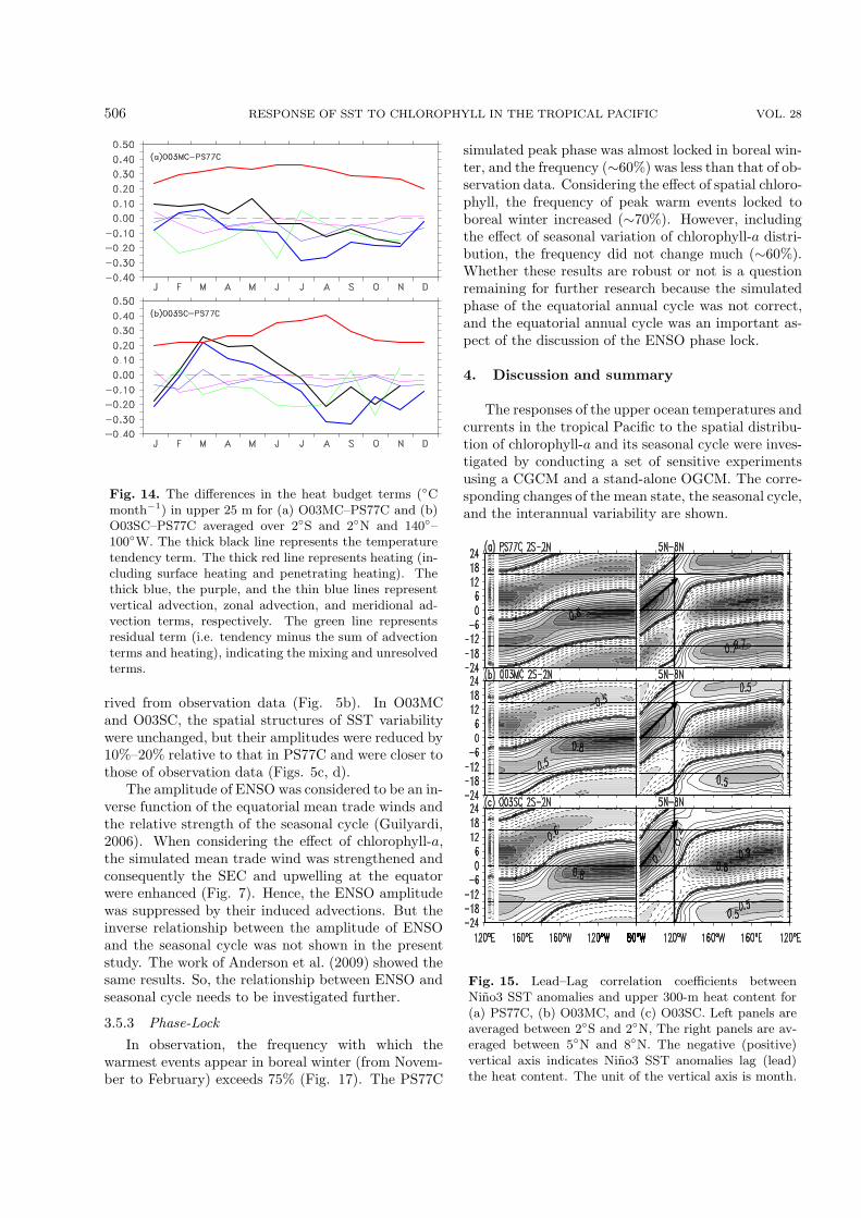
Fig. 12. The differences in the heat budget terms (◦Cmonth−1) between depth 62.5 m and 112.5 m for (a)O03MC–PS77C and (b) O03SC–PS77C averaged over140◦–120◦W and 10◦–15◦N. The thick black line rep-resents temperature tendency term. The thick red lineis for penetrating heating. The thick blue, the purple,and the thin blue lines represent vertical advection, zonaladvection, and meridional advection terms, respectively.The green line represents residual term (i.e., tendency mi-nus the sum of advection terms and heating), indicatingthe mixing and unresolved terms.

O03MC.Compared with PS77C, zonal averaged SSTs in

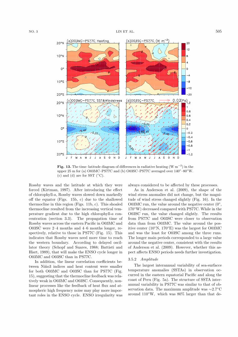
both O03MC and O03SC decreased in all seasons inthe equatorial eastern Pacific (Figs. 13c, d). SST de-creased more obviously from September to May. More-over, the SST decrease in O03SC was larger than thatin O03MC, especially from January to May. Sincemore solar radiation was absorbed in the upper layerall year around (Fig. 13a), the amplitude of the SSTdecrease was reduced (Fig. 13c) in O03MC. In O03SC,the amplitude of the SST decrease was also associ-ated with the solar radiative heating. Because theseasonal cycle of chlorophyll-a was adopted in O03SC,the seasonal difference in radiative heating came fromnot only the seasonal cycle of shortwave radiation butalso the seasonal cycle of chlorophyll-a (Fig. 13b).Large radiative heating occurred only in boreal sum-mer, where the large chlorophyll-a concentration ex-ists. Hence, the SST in the eastern equatorial Pacificfor O03SC was much colder than that for O03MC.

Evaluation of the near-surface temperature heatbudget (Fig. 14) indicates that the heating termincluding surface forcing and penetrating heating

warms the temperature. The near-surface tempera-ture warmed from January to June in O03MC butlasted until July in O03SC. After that, the temper-ature started to cool. The tendency term changedwith vertical advection, especially in O03SC. Verticaladvection contributed to cooling from July to Decem-ber. The other terms (the zonal advection, meridionaladvection, and the residual term) can contribute tothe temperature variation at times. Interestingly, theresidual term cannot be omitted. The slight local windvariation cannot explain the temperature and currentvariation at the equator. The heating difference dueto chlorophyll-a concentration was the initial induce-ment. The heating at the sea surface and cooling atdeeper depth increased the vertical temperature gra-dient (i.e., more stable stratification) and enhancedvertical advection. Although vertical advection canexplain most of the temperature variation, other heat-budget terms are at work at times.

3.5 Effect of annual mean and seasonal cycleof chlorophyll-a on interannual variability

3.5.1 Frequency

Chlorophyll-a can affect not only mean state andseasonal variation in the tropical Pacific but also in-terannual variability. Figure 6 shows the time seriesof Nino3 indices and their power spectrums both forthe observation data and for the coupled experiments.The observed ENSO periods exhibit two frequencybands: 2–4 years and 4–6 years (Fig. 6b). How-ever, the PS77C has only one sharp peak at 3.3 years.Due to the large amplitude of ENSO in FGOALS-g1.1(Fig. 6), the energy for PS77C is about twice thatof observation data. After introducing the effect ofchlorophyll-a, more spectral peaks appeared. In ad-dition to the peak at ∼3 years for O03MC, anotherpeak occurred with a period of ∼4–6 years. In O03SC,the dominating period shifted to 4 years, and anothersignificant period for O03SC occurred with a periodof ∼6–8 years. The corresponding energy at the domi-nant peak in O03MC was almost unchanged relative toPS77C, while it was reduced by 30% in O03SC. There-fore, when considering the influence of chlorophyll-a, ENSO in the coupled model became more irregu-lar and the amplitudes also decreased, especially inO03SC. In turn, that led the simulated characteris-tics of ENSO to be much closer to the observationdata. Enhancement of the irregularity of ENSO dueto change of the solar radiation penetration depth hasalso been reported in previous studies (Wetzel et al.,2006; Ballabrera-Poy et al., 2007; Anderson et al.,2007; Lengaigne et al., 2007).

The ENSO period can be affected by off-equatorial


Fig. 13. The time–latitude diagram of differences in radiative heating (W m−2) in theupper 25 m for (a) O03MC–PS77C and (b) O03SC–PS77C averaged over 140◦–80◦W.(c) and (d) are for SST (◦C).

Rossby waves and the latitude at which they wereforced (Kirtman, 1997). After introducing the effectof chlorophyll-a, Rossby waves slowed down markedlyoff the equator (Figs. 15b, c) due to the shallowedthermocline in this region (Figs. 11b, c). This shoaledthermocline resulted from the increasing vertical tem-perature gradient due to the high chlorophyll-a con-centration (section 3.3). The propagation time ofRossby waves across the eastern Pacific in O03MC andO03SC were 2–4 months and 4–6 months longer, re-spectively, relative to those in PS77C (Fig. 15). Thisindicates that Rossby waves need more time to reachthe western boundary. According to delayed oscil-lator theory (Schopf and Suares, 1988; Battisti andHisrt, 1989), that will make the ENSO cycle longer inO03MC and O03SC than in PS77C.

In addition, the linear correlation coefficients be-tween Nino3 indices and heat content were smallerfor both O03MC and O03SC than for PS77C (Fig.15), suggesting that the thermocline feedback was rela-tively weak in O03MC and O03SC. Consequently, non-linear processes like the feedback of heat flux and at-mospheric high frequency noise may play more impor-tant roles in the ENSO cycle. ENSO irregularity was

always considered to be affected by these processes.As in Anderson et al. (2009), the shape of the

wind stress anomalies did not change, but the magni-tude of wind stress changed slightly (Fig. 16). In theO03MC run, the value around the negative center (0◦,170◦W) decreased compared with PS77C. While in theO03SC run, the value changed slightly. The resultsfrom PS77C and O03SC were closer to observationdata than from O03MC. The value around the pos-itive center (10◦N, 170◦E) was the largest for O03MCand was the least for O03SC among the three runs.The longer main periods corresponded to a large valuearound the negative center, consistent with the resultsof Anderson et al. (2009). However, whether this as-pect affects ENSO periods needs further investigation.

3.5.2 AmplitudeThe largest interannual variability of sea-surfacce

temperature anomalies (SSTAs) in observation oc-curred in the eastern equatorial Pacific and along thecoast of Peru (Fig. 5a). The structure of SSTA inter-annual variability in PS77C was similar to that of ob-servation data. The maximum amplitude was ∼2.7◦Caround 110◦W, which was 80% larger than that de-


Fig. 14. The differences in the heat budget terms (◦Cmonth−1) in upper 25 m for (a) O03MC–PS77C and (b)O03SC–PS77C averaged over 2◦S and 2◦N and 140◦–100◦W. The thick black line represents the temperaturetendency term. The thick red line represents heating (in-cluding surface heating and penetrating heating). Thethick blue, the purple, and the thin blue lines representvertical advection, zonal advection, and meridional ad-vection terms, respectively. The green line representsresidual term (i.e. tendency minus the sum of advectionterms and heating), indicating the mixing and unresolvedterms.

rived from observation data (Fig. 5b). In O03MCand O03SC, the spatial structures of SST variabilitywere unchanged, but their amplitudes were reduced by10%–20% relative to that in PS77C and were closer tothose of observation data (Figs. 5c, d).

The amplitude of ENSO was considered to be an in-verse function of the equatorial mean trade winds andthe relative strength of the seasonal cycle (Guilyardi,2006). When considering the effect of chlorophyll-a,the simulated mean trade wind was strengthened andconsequently the SEC and upwelling at the equatorwere enhanced (Fig. 7). Hence, the ENSO amplitudewas suppressed by their induced advections. But theinverse relationship between the amplitude of ENSOand the seasonal cycle was not shown in the presentstudy. The work of Anderson et al. (2009) showed thesame results. So, the relationship between ENSO andseasonal cycle needs to be investigated further.

3.5.3 Phase-LockIn observation, the frequency with which the

warmest events appear in boreal winter (from Novem-ber to February) exceeds 75% (Fig. 17). The PS77C

simulated peak phase was almost locked in boreal win-ter, and the frequency (∼60%) was less than that of ob-servation data. Considering the effect of spatial chloro-phyll, the frequency of peak warm events locked toboreal winter increased (∼70%). However, includingthe effect of seasonal variation of chlorophyll-a distri-bution, the frequency did not change much (∼60%).Whether these results are robust or not is a questionremaining for further research because the simulatedphase of the equatorial annual cycle was not correct,and the equatorial annual cycle was an important as-pect of the discussion of the ENSO phase lock.

4. Discussion and summary

The responses of the upper ocean temperatures andcurrents in the tropical Pacific to the spatial distribu-tion of chlorophyll-a and its seasonal cycle were inves-tigated by conducting a set of sensitive experimentsusing a CGCM and a stand-alone OGCM. The corre-sponding changes of the mean state, the seasonal cycle,and the interannual variability are shown.

Fig. 15. Lead–Lag correlation coefficients betweenNino3 SST anomalies and upper 300-m heat content for(a) PS77C, (b) O03MC, and (c) O03SC. Left panels areaveraged between 2◦S and 2◦N, The right panels are av-eraged between 5◦N and 8◦N. The negative (positive)vertical axis indicates Nino3 SST anomalies lag (lead)the heat content. The unit of the vertical axis is month.


Fig. 16. The magnitude of wind stress (mPa) (December–January–February) regressed on Nino3SST anomalies for (a) ERA40, (b) PS77C, (c) O03MC, and (d) O03SC.

When introducing the spatial distribution ofchlorophyll-a in models, the annual mean SST in theeastern equatorial Pacific decreased accompanied by amore shallow thermocline and stronger currents. Theupper layer heat budget in the cold tongue region wasmainly controlled by upwelling. The vertical advec-tive cooling cancelled out the radiative heating dueto the high chlorophyll-a concentration. Comparisonbetween the results from the CGCM and the OGCMindicate that the atmosphere-ocean interaction, suchas Bjerknes or the Wind-Evaporation-SST feedback,further enhances the cooling in the eastern equatorialPacific.

Fig. 17. The frequency distribution (%) as a function ofthe month in which the peak ENSO warm events appear.

Both the spatial distribution of chlorophyll-a andits seasonal cycle did not change the phase of the SSTseasonal cycle in the cold tongue. They only slightlyenhance the amplitude of the seasonal cycle. How-ever, the seasonal cycle of chlorophyll-a did dramati-cally change the period of ENSO in the coupled model.The power spectrum analysis showed that the peakof the spectrum became broad and that a longer pe-riod was found after the seasonal cycle of chlorophyll-a distribution was introduced. These changes led toENSO irregularities in the model. The increasingENSO period was mainly due to the slow speed ofRossby waves, which were mainly caused by the de-creased depth of the thermocline in the northeasternPacific. The change in the wind magnitude may alsohave contributed to the change of ENSO periods.

In the present study, the annual mean SST in east-ern equatorial Pacific decreased due to the shallowpenetration depth of radiative heating caused by thedistribution of chlorophyll-a, consistent with Ander-son et al. (2007), Ballabrera-Poy et al. (2007), andGnanadesikan and Anderson (2009). But other stud-ies had also shown warm SSTs in the cold tongue re-gion (Wetzel et al., 2006; Lengaigne et al., 2007). Inaddition to the direct heating due to the increasingchlorophyll-a in the cold tongue, the SST was alsocontrolled by the equatorial upwelling. This local up-welling had the ability to cool the SST in the region.Cooling can be amplified by positive feedback (i.e.,


Fig. 18. The time-period diagram of wavelet coefficient (amplitudes) for PS77C Nino3 in-dex. The y-axis is the period (years), and the x-axis is for years. The red dashed linerepresents the 5% significance test.

Fig. 19. (a) Annual mean SST difference for two time periods (L3–L1). L1 is from modelyear 2061 to model year 2095. L2 is from model year 2096 to model year 2123. L3 is frommodel year 2124 to model year 2139. (b) The same as (a) except for the thermocline (i.e.,the depth of the 20◦C isotherm).

Bjerknes feedback) in the coupled model. As suggestedby previous OGCM studies (e.g., Sweeney et al., 2005;Anderson et al., 2007; Lin et al., 2008), the cooling inthe cold tongue due to change of chlorophyll-a concen-tration was a primary attribute of the cold upwellingdue to the cold water from the off-equatorial regionbelow the mixed layer. That is, the change of SSTin this region was a result of the competition betweenthe direct heating and the advective cooling, includinglocal and remote effects. So if the former was strong ina model, the sensitive experiments will show a warmSST in the cold tongue region, and if the latter wasstrong in a model, the sensitive experiments will showa cold SST in the cold tongue region.

The ENSO periods in FGOALS-g1.1 also haddecadal variability. Figure18 showed the time-perioddiagram of wavelet coefficient of the Nino3 index inPS77C. During years 2061–2095 (L1), the ENSO pe-riod was 3–4 years, and the amplitude was strong.During years 2096–2123 (L2), however, the ENSO pe-riod did not change much, and the amplitude weak-ened. From 2124 to 2139 (L3), the ENSO periodwas ∼4 years, and the amplitude became large again.

The decadal change in FGOALS-g1.1 was associatedwith the change in mean climate background. Fig-ure 19 showed the differences of SST and thermoclinedepth, which was defined as the 20◦C isotherm, be-tween L1 and L3. The changes in SST, thermocline,and ENSO period were consistent with the change in-cluding the effect of chlorophyll-a concentration (oceancolor). This indicates that the relationship betweenthe ENSO period and the mean state was robust inFGOALS-g1.1. This kind of relationship can also befound when the shortwave-radiation penetration depthchanges due to chlorophyll-a distribution.

Does the decadal variability of ENSO in FGOALSaffect our results? We also computed the power spec-trum of Nino3 index for O03MC and O03SC using thelast 80-year integration (not shown). Although the ex-act period was different using the 30-year integration,they were qualitatively the same. The period of ENSOalso became longer and more irregular in the 80-yearintegrations done using O03MC and O03SC. So thedecadal variability of ENSO did change our conclu-sions.

In this study, the mean and seasonal cycle of


chlorophyll-a concentration (ocean color) were usedto investigate the response of temperature and cur-rent in the tropical Pacific. As known to us, be-sides the seasonal variation of ocean color, there wasstrong interannual variability of chlorophyll-a concen-tration (ocean color) associated with interannual vari-ability of physical fields. The present study overesti-mated chlorophyll-a concentration during warm ENSOphases and underestimated it during cold ENSOphases. How these variations affect the temperatureand current were matters for further investigation.

As shown above, FGOALS-g1.1 has biases not onlyin the mean state but also in the seasonal cycle and ininterannual variability. Some of them were common;some were unique. So far we cannot clearly under-stand the impact of these biases on our results. Theonly thing we can do was to compare our results withresults from other coupled GCMs and to find differ-ences that are reasonable and understandable. Thecomparison with Wetzel et al. (2006), Anderson et al.(2007), Ballabrera-Poy et al. (2007), and Lengaigne etal. (2007) indicated that two changes in our study wererelatively robust: the cooling in the eastern equatorialPacific and the increasing irregularity of ENSO due tothe effect of chlorophyll-a distribution.

Acknowledgements. We wish to thank the two

anonymous reviewers for their very valuable comments that

helped to improve our paper. This study is jointly sup-

ported by the National Basic Research Program of China

(also called 973 Program, Grant Nos. 2010CB428904,

2007CB411806, 2006CB403600), the National Natural Sci-

ence Foundation of China under Grant Nos. 40775054,

40906012.

REFERENCES

Anderson, W. G., A. Gnanadesikan, R. Hallberg, J.Dunne, and B. L. Samuels, 2007: Impact of oceancolor on the maintenance of the Pacific Cold Tongue.Geophys. Res. Lett., 34, L11609: doi:10.1029/2007GL030100.

Anderson, W. G., A. Gnanadesikan, and A. Wittenberg,2009: Regional impacts of ocean color on tropicalPacific variability. Ocean Science, 5, 313–327.

Ballabrera-Poy, J., R. Murtugudde, R. H. Zhang, and A.J. Busalacchi, 2007: Coupled ocean–atmosphere re-sponse to seasonal modulation of ocean color: Impacton interannual climate simulations in the TropicalPacific. J. Climate, 20, 353–374.

Battisti, D. S., and A. C. Hisrt, 1989: Interannual vari-ability in a tropical atmosphere-ocean model: in-flunce of the basic state, ocean geometry and non-linearity. J. Atmos. Sci., 46, 1687–1712.

Bjerknes, J., 1969: Atmospheric teleconnections from theequatorial Pacific. Mon. Wea. Rev., 97, 163–172.

Collins, W. D., and Coauthors, 2003: Description of theNCAR Community Atmosphere Model (CAM2). Na-tional Center of Atmospheric Research,Boulder, CO,171pp.

Gent, P. R., and J. C. McWilliams, 1990: Isopycnal mix-ing in ocean circulation models. J. Phys. Oceanogr.,20, 150–155.

Gnanadesikan, A., and W. G. Anderson, 2009: Oceanwater clarity and the ocean general circulation in acoupled climate model. J. Phys. Oceanogr., 39, 314–332.

Guilyardi, E., 2006: El Nino–mean state–seasonal cy-cle interactions in a multi-model ensemble. ClimateDyn., 26, 329–348.

Kiehl, J. T., and P. R. Gent, 2004: The community cli-mate system model, version 2. J. Climate, 17, 3666–3682.

Kirtman, B. P., 1997: Oceanic Rossby wave dynamics andthe ENSO period in a coupled model. J. Climate, 10,1690–1704.

Latif, M., and Coauthors, 2001: ENSIP: The El Ninointercomparison project. Climate Dyn., 18, 255–276.

Lengaigne, M., C. Menkes, O. Aumont, T. Gorgues, L.Bopp, J. M. Andre, and G. Madec, 2007: Influenceof the oceanic biology on the tropical Pacific climatein a coupled general circulation model. Climate Dyn.,28, 503–516, doi: 10.1007/s00382-006-0200-2.

Lewis, M. R., M. E. Carr, G. C. Feldman, W. Esias, andC. McClain, 1990: Influence of penetrating solar ra-diation on the heat budget of the equatorial PacificOcean. Nature, 347, 543–545.

Lin, J. L., 2007: The double-ITCZ problem in IPCC AR4coupled GCMs: Ocean-atmosphere feedback analy-sis. J. Climate, 20, 4497–4525.

Lin, P. F., H. L. Liu, and X. H. Zhang, 2007: Sensitivityof the upper ocean temperature and circulation inthe equatorial Pacific to solar radiation penetrationdue to phytoplankton. Adv. Atmos. Sci., 24, 765–780, doi: 10.1007/s00376-007-0765-7.

Lin, P. F., H. L. Liu, and X. H. Zhang, 2008: Effect ofchlorophyll-a horizontal distribution on upper oceantemperature in the central and eastern equatorial Pa-cific. Adv. Atmos. Sci., 25, 585–596.

Liu, H. L., Y. Q. Yu, W. Li, and X. H. Zhang, 2004a:Manual for LASG/IAP Climate System Ocean Model(LICOM1.0). Science Press, Beijing, 1–128. (in Chi-nese)

Liu, H. L., X. H. Zhang, W. Li, Y. Q. Yu, and R. C.Yu, 2004b: A eddy-permitting oceanic general cir-culation model and its preliminary evaluations. Adv.Atmos. Sci., 21, 675–690.

Manizza, M., C. Le Quere, A. J. Watson, and E. T.Buitenhuis, 2005: Bio-optical feedbacks among phy-toplankton, upper ocean physics and sea-ice in aglobal model. Geophys. Res. Letts., 32, L05603, doi:10.1029/2004GL020778.

Mechoso, C. R., and and Coauthors, 1995: The sea-sonal cycle over the tropical Pacific in coupled ocean–atmosphere general circulation models. Mon. Wea.


Rev., 123, 2825–2838.Murtugudde, R., J. Beauchamp, C. R. McClain, M.

Lewis, and A. J. Busalacchi, 2002: Effects of pen-etrative radiation on the upper tropical ocean circu-lation. J. Climate, 15, 470– 486.

Nakamoto, S., S. P. Kumar, J. M. Oberhuber, J. Ishizaka,K. Muneyama, and R. Frouin, 2001: Response of theequatorial Pacific to chlorophyll pigment in a mixedlayer isopycnal ocean general circulation model. Geo-phys. Res. Letts., 28(10), 2021–2024.

Ohlmann, J. C., 2003: Ocean radiant heating in climatemodels. J. Climate, 16, 1337–1351.

Pacanowski, R. C., and S. G. H. Philander, 1981: Param-eterization of vertical mixing in numerical models oftropical oceans. J. Phys. Oceanogr., 11, 1443–1451.

Paulson, C. A., and J. J. Simpson, 1977: Irradiance mea-surements in the upper ocean. J. Phys. Oceanogr., 7,952–956.

Pennington, J. T., K. L. Mahoney, V. S. Kuwahara, D.D. Kolber, R. Calienes, and F. P. Chavez, 2006: Pri-mary production in the eastern tropical Pacific: Areview. Prog. Oceanogr., 69, 285–317.

Reynolds, R. W., and T. M. Smith, 1994: Improved globalsea surface temperature analyses using optimum in-terpolation. J. Climate, 7, 929–948.

Roske, F., 2001: An atlas of surface fluxes based onthe ECMWF re-analysis—A climatological datasetto force global ocean general circulation models. Re-port No. 323, MPI, Hamburg, Germany, 31pp.

Rosati, A., and K. Miyakoda, 1988: A general circu-lation model for upper ocean simulation. J. Phys.Oceanogr., 18, 1601–1626.

Sathyendranath, S., A. D. Gouveia, S. R. Shetye, P.Ravindran, and T. Platt, 1991: Biological controlof surface temperature in the Arabian Sea. Nature,349, 54–56.

Schneider, E. K., and Z. Zhu, 1998: Sensitivity of thesimulated annual cycle of sea surface temperature inthe equatorial Pacific to sunlight penetration. J. Cli-mate, 11, 1932–1950.

Schopf, P. S., and M. J. Suares, 1988: Vacillations ina coupled ocean–atmosphere model. J. Atmos. Sci.,45, 549–566.

Siegel, D. A., J. C. Ohlmann, L. Washburn, R. R. Bidi-gare, C. Nosse, E. Fields, and Y. Zhou, 1995: Solarradiation, phytoplankton pigments and radiant heat-

ing of the equatorial Pacific warm pool. J. Geophys.Res., 100, 4885–4891.

Strutton, P., and F. P. Chavez, 2004: Biological heatingin the equatorial Pacific: Observed variability andpotential for real-time calculation. J. Climate, 17,1097–1109.

Sweeney, C., A. Gnanadesikan, S. M. Griffies, M. J. Har-rison, A. J. Rosati, and B. L. Samuels, 2005: Impactsof shortwave penetration depth on large-scale oceancirculation and heat transport. J. Phys. Oceanogr.,35, 1103–1119.

Uppala, S., and Coauthors, 2005: The era-40 re-analysis.Quart. J. Roy. Meteor. Soc., 131, 2961–3012.

Wang, B., H. Wan, Z. Z. Ji, X. Zhang, R. C. Yu, Y. Q.Yu, and H. T. Liu, 2004: Design of a new dynamicalcore for global atmospheric models based on some ef-ficient numerical methods. Science in China(A), 47,4–21.

Wetzel, P., E. Maier-Reimer, M. Botzet, J. Jungclaus, N.Keenlyside, and M. Latif, 2006: Effects of ocean biol-ogy on the penetrative radiation in a coupled climatemodel. J. Climate, 19, 3973–3987.

Xie, S. P., 1994: On the genesis of the equatorial annualcycle. J. Climate, 7, 2008–2013.

Xie, S. P., 2004: The shape of continents, air–sea interac-tion, and the rising branch of the Hadley circulation.The Hadley Circulation: Past, Present and Future,H. F. Diaz and R. S. Bradley, Eds., Kluwer Aca-demic, Dordrecht, 121–152.

Yu, L., X. Jin, and R. A. Weller, 2008a: MultidecadeGlobal Flux Datasets from the Objectively Ana-lyzed Air–sea Fluxes (OAFlux) Project: Latent andsensible heat fluxes, ocean evaporation, and relatedsurface meteorological variables. OA-2008-1, WoodsHole Oceanographic Institution, 64pp.

Yu, Y., and D. Sun, 2009: Response of ENSO and themean state of the tropical Pacific to extratropicalcooling/warming: A study using the IAP coupledmodel. J. Climate, 22, 5902–5917.

Yu, Y., W. Zheng, X. Zhang, and H. Liu, 2007: LASGcoupled climate system model FGCM-1.0. Chinese J.Geophys., 50(6), 1677–1687.

Yu, Y., and Coauthors, 2008b: Coupled model sim-ulations of climate changes in the 20th centuryand beyond. Adv. Atmos. Sci., 25, 641–654, doi:10.1007/S00376-008-0641-0.

response of sea surface temperature to chlorophyll...

Documents