HAL Id: hal-00769274https://hal.archives-ouvertes.fr/hal-00769274v3

Submitted on 27 Nov 2014

HAL is a multi-disciplinary open accessarchive for the deposit and dissemination of sci-entific research documents, whether they are pub-lished or not. The documents may come fromteaching and research institutions in France orabroad, or from public or private research centers.

L’archive ouverte pluridisciplinaire HAL, estdestinée au dépôt et à la diffusion de documentsscientifiques de niveau recherche, publiés ou non,émanant des établissements d’enseignement et derecherche français ou étrangers, des laboratoirespublics ou privés.

Response of an artificially blown clarinet to differentblowing pressure profiles

Baptiste Bergeot, André Almeida, Christophe Vergez, Bruno Gazengel,Ferrand Didier

To cite this version:Baptiste Bergeot, André Almeida, Christophe Vergez, Bruno Gazengel, Ferrand Didier. Response ofan artificially blown clarinet to different blowing pressure profiles. Journal of the Acoustical Societyof America, Acoustical Society of America, 2014, 135 (1), pp.479-490. �10.1121/1.4835755�. �hal-00769274v3�

Response of an artificially blown clarinet to different blowing pressureprofiles

B. Bergeota,b,∗, A. Almeidaa,c, C. Vergezb, B. Gazengela and D. Ferrandd

aLUNAM Université, Université du Maine, UMR CNRS 6613, Laboratoire d’Acoustique, Avenue Olivier Messiaen,72085 Le Mans Cedex 9, FrancebLMA, CNRS UPR7051, Aix-Marseille Univ., Centrale Marseille, F-13402 Marseille Cedex 20, Francec School of Physics, The University of New South Wales, Sydney UNSW 2052, Australiad Laboratoire d’Astrophysique de Marseille (LAM-CNRS-INSU UMR 7326), Pôle de l’Étoile Site de Château-Gombert / 38, rue FrédéricJoliot-Curie 13388 Marseille Cedex 13, France

∗ Corresponding author, baptiste.bergeot@centrale-marseille.fr

Abstract. Using an artificial mouth with an accurate pressurecontrol, the onset of the pressure oscillations inside the mouth-piece of a simplified clarinet is studied experimentally. Twotime profiles are used for the blowing pressure: in a first setof experiments the pressure is increased at constant rates, thendecreased at the same rate. In a second set of experiments thepressure rises at a constant rate and is then kept constant foran arbitrary period of time. In both cases the experiments arerepeated for different increase rates.

Numerical simulations using a simplified clarinet modelblown with a constantly increasing mouth pressure are com-pared to the oscillating pressure obtained inside the mouthpiece.Both show that the beginning of the oscillations appears at ahigher pressure values than the theoretical static threshold pres-sure, a manifestation of bifurcation delay.

Experiments performed using an interrupted increase inmouth pressure show that the beginning of the oscillation occursclose to the stop in the increase of the pressure. Experimentalresults also highlight that the speed of the onset transient of thesound is roughly the same, independently of the duration of theincrease phase of the blowing pressure.

Keywords: Musical acoustics, Clarinet-like instruments,Transient processes, Iterated maps, Dynamic Bifurcation, Bifur-cation delay.

1 Introduction

The clarinet is one of the most well-described instrument interms of scientific theories for its behavior. The relative simplic-ity of its elements and their couplings has allowed to explainseveral features of the sustained sound of the clarinet, such asthe playing frequency, the harmonic content, or the amplitudeof the sound, and their variation with the action of the musicianon its instrument. An important part of the timbre of this musi-cal instrument can thus be understood with currently existingmodels. However, the timbre does not only depend on the char-acteristics of the sustained sound but to a great extent, on thequick variations that happen at the onset of the sound, i. e., theattack transient.

The first studies [1, 2, 3, 4, 5, 6] concerning the clarinet as-sume that the mouth pressure is constant and does not depend ontime. We call this approach the “static case”. These studies usesimple resonator models (single mode [1], iterated map[2, 3] orcontinuation methods of the Hopf bifurcation[7]) and a linearapproximation of the non-linear characteristic function of theexciter to predict the threshold pressure, the bifurcation diagramand the temporal shape of the pressure inside the mouthpiece.Results show that the oscillation threshold pressure, which willbe called in this article the “static oscillation threshold” is re-lated to reed stiffness, the mouthpiece opening and the lossesinside the resonator [4, 2]. The calculated and the measuredthresholds show qualitative agreement if the threshold pressureis measured while the mouth pressure is slowly decreasing [5].Prediction of the transient using a linearization of the excitercharacteristic agrees well with numerical simulations [1] andshows that the acoustic pressure starts with an exponential en-velope before reaching saturation [6]. For a given resonatorand a fixed embouchure, the γ coefficient of the exponentialgrowth (p0eγt) depends only on the value of the constant mouthpressure.

In a real situation, the attack of a note is produced with acomplex combined action of several gestures. In special occa-sions, a musician will perform a “breath attack” without usinghis tongue. These transients show that the mouth pressure in-creases quickly, typically in 40ms [8] and that players overshoota desired blowing pressure and then “decay” back to a “sustain”level.

More recent articles have studied the behavior of the instru-ment for time-varying pressures. Typically, these have used“Continuous Increasing Mouth Pressure” (CIMP), in which theblowing pressure increases with time at a constant rate, and“Interrupted Increasing Mouth Pressure followed by a Plateau”(IIMPP), in which the constant increase is stopped at the “in-terrupting time”, being followed by a constant pressure. Usinga CIMP, Atig et al [9] notices that oscillation threshold pres-sure calculated using numerical simulation is higher than thestatic oscillation threshold. Bergeot et al [10] provide an ana-lytical/numerical study of a simple clarinet model (also usedin this paper and presented in section 3) in CIMP situationsand propose the term “dynamic oscillation threshold” to define

1

the beginning of mouthpiece pressure oscillation in dynamiccases. An analytical expression is proposed for the dynamicthreshold, predicting that it is always higher than the “staticthreshold”. This phenomenon is known in mathematical litera-ture as bifurcation delay [11]. We wish to emphasize that theterm “delay” in bifurcation delay does not necessarily refer to atime difference but to a shift in the oscillation threshold. In thiswork, the word “delay” often refers to that shift.

The comparison between theoretical results and numericalsimulations reveals an important sensitivity to the precision (i.e.the number of digits) used in numerical simulations. Indeed,numerical results only converge to the theory when the sim-plified model (the same as used for analytical investigation) iscomputed with hundreds or thousands of digits [10]. Otherwise,theoretical results become useless in predicting the behaviorof the simulated model. In this case, the dynamic thresholdincreases with the increase rate of the mouth pressure. Silva[12] performs numerical simulations of an IIMPP, showing thatthe beginning of the envelope of the mouthpiece pressure is anexponential p0eγt arising once the mouth pressure stops increas-ing, and in which the growth constant γ does not depend on theduration of the mouth pressure increase.

In this paper, the operation of a simplified clarinet under sim-plified conditions (CIMP and IIMPP mouth pressure profiles)is studied experimentally. The “clarinet” is a simple cylindricaltube attached to a clarinet mouthpiece – it has no bore variations,no flare, no bell and no tone or register holes.

To characterise the onset, three main parameters will be used:the time (or value of mouth pressure) at the start of the oscilla-tions, their initial amplitude, and the growth constant (which aswill be seen, can be vary through time in some cases). Theseparameters can be equivalently expressed as a function of timeor as a function of mouth pressure, since the latter is an affinefunction of time.

In the case of the CIMP profile, these parameters, measuredusing the artificial mouth, are compared to the parameters es-timated using simulations of a simplified clarinet model fordifferent values of the increase rate of the CIMP.

In the case of the IIMPP, the starting time of the oscillationsand the growth constant are related to the characteristics of themouth pressure profile, in particular the “interrupting time” ofthe IIMPP, and the value of constant pressure reached at the endof the IIMPP.

The paper is organized as follows: section 2 presents theexperimental system (artificial mouth). Section 3 presents thephysical model used for simulating the clarinet system. Theexperimental results are presented and discussed in section 4for CIMP profiles and in section 5 for IIMPP profiles of mouthpressure. In section 4 experimental results obtained for CIMPprofiles are compared to numerical simulations.

2 Experimental setup and configurations

We describe here the experimental setup and the two experi-mental protocols used in the work. An outline schematic of theexperimental setup is presented in fig. 1.

Barrel Resonator

Mouthpiece

pressure sensorMouth pressure

sensor

Plexyglas box

(Arti�cial mouth)Arti�cial lip

Flowmeter

Air TankServo

Valve

Computer

+

dSpace

Hardware

Pressure

Reducer

Compressed

Air

(≈ 6 .105 Pa)

Mouthpiece

Figure 1: Principle of the Pressure Controlled Artificial Mouth(PCAM).

2.1 Materials

A simplified clarinet is inserted by its mouthpiece into PressureControlled Artificial Mouth (PCAM). The PCAM is responsiblefor controlling the mouth pressure and provides a suitable sup-port for the sensors used in measuring the physical quantities ofinterest[13, 14].

The simplified clarinet is made of a plastic cylinder connectedto the barrel of a real clarinet. The total length of cylinder andbarrel is l = 0.52m (this is also the effective length of theinstrument, calculated from L = c/4f , where c is the soundvelocity and f the playing frequency) and the internal diameteris 15mm.

The artificial mouth is made of a Plexiglas box which supportsrigidly both the mouthpiece and the barrel. It is a chamber withan internal volume of 30cm3 where the air pressure Pm is to becontrolled. The artificial lip is made of a foam pad sitting on thereed.

Both the internal mouth pressure and the pressure inside themouthpiece are measured using differential pressure sensors(Endevco 8510B and 8507C respectively). Finally, a flowmeter(Bürkert 8701) is placed at the entrance of the artificial mouth tomeasure the input volume flow entering into the reed channel.

Control of the mouth pressure is based on high-precisionregulation of the air pressure inside the Plexiglas box. This reg-ulation enables the control of blowing pressure around a targetwhich can either be a fixed value or follow a function varyingslowly over time. A servo-valve (Bürkert 2832) is connectedto a compressed air source through a pressure reducing valve.The servo valve is a proportional valve in which the openingis proportional to the electric current. The maximum pressureavailable is approximately 6 · 105Pa. A pressure reducer isused to adjust the pressure upstream the servo-valve which isconnected to the entrance of the artificial mouth itself. An airtank (120 litres) is inserted between of the servo-valve and the

2

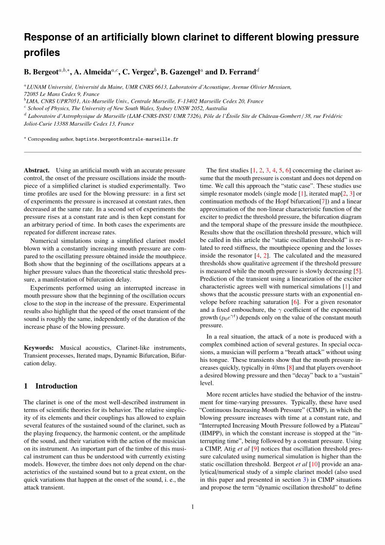
Figure 2: Time evolution of the mouth pressure Pm(t) (CIMP profile)and of the pressure inside the mouthpiece P (t). The slope k of themouth pressure is equal to 0.1 kPa/s.

Table 1: Estimation of the slope for each repetition in experiment plusaverages.

Experiment 1 2 3 4 5 6Values of k (kPa/s) (incr. blowing pressure)1st time 0.100 0.140 0.233 0.751 1.557 2.6812nd time 0.100 0.140 0.233 0.752 1.557 2.7123rd time 0.100 0.140 0.233 0.753 1.559 2.711Average 0.100 0.140 0.233 0.752 1.558 2.702

artificial mouth in order to stabilize the feedback loop duringslowly varying onsets. This large tank is used for experimentsperformed with the CIMP profile, and is replaced by a muchsmaller tank (approx. 2 litres) when faster varying targets aretested (IIMPP profile). The control algorithm is implementedon a DSP card (dSpace DS1104), modifying the volume flowthrough the servo-valve every 40µs in order to minimize thedifference between the measured and the target mouth pressure.Moreover, because of the long response time of the flowmeter,the volume flow is measured but is not used in the control loop.

2.2 Experimental protocol

2.2.1 "CIMP" profile

Starting from a low value (0.2 kPa in our experiment) the mouthpressure Pm(t) is increased at a constant rate k (the slope) untila few seconds after the clarinet starts to sound. The mouthpressure is then decreased with a symmetric slope (k′ = −k).During the experiment, the mouth pressure Pm(t), the pressurein the mouthpieceP (t) and the incoming flowU(t) are recorded.Fig. 2 shows an example of the time profile of Pm and P withk = 0.1 kPa/s.

The experiment is repeated three times for each of the targetslope values k given as a command to the PCAM. The actualvalues of the slope obtained during the experiment are estimatedusing a linear fit and shown in table 1. We can see that theuse of the PCAM provides a very good repeatability on theincrease/decrease rate of the blowing pressure.

� ��� ��� ��� ��� � �����

��

��

�

�

�

�

�

T��e (��

P�������Pa�

M �������� �p����p� � ���

B w�!g �p����p� �"���

#$%&'i)* +i,%

-./012

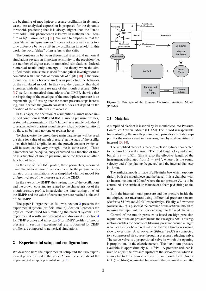
Figure 3: Measured signals in an IIMPP case: blowing pressure Pm(t)(solid black line) and pressure inside the mouthpiece P (t) (solid grayline).

2.2.2 "IIMPP" profile

For the IIMPP profile, the blowing pressure has two phases, firstincreasing at a faster rate than that used for the CIMP profile,then kept at an almost constant value. For example, in fig. 3, theblowing pressure Pm starts at a low value (approx. 0.1 kPa), in-creases for a certain time (hereafter referred as (∆t)Pm

), reachesa target value (approx. 7 kPa) and is then kept constant. Theexperiment is repeated for different values of (∆t)Pm

(targetvalues are 0.05s, 0.2s, 0.5s and 1s corresponding respectivelyto experiments numbered 1, 2, 3 and 4, cf. table 2) and re-peated fifteen times for each value of (∆t)Pm

. Table 2 shows agood agreement between the command and the measurementof (∆t)Pm

. This indicates that the control of the PCAM workseven for rapid variations in blowing pressure. However, forthe fastest (experiment 1), the difference between the commandand measurement is about 50% of the command. Table 2 alsoshows good repeatability of the blowing pressure slope duringthe increasing part.

In this experiment, only the blowing pressure Pm and theinternal mouthpiece pressure P are recorded (see fig. 3).

3 Clarinet model

This section presents the physical model of the clarinet usedin this work. The numerical simulations of the model will becompared to experimental results in section 4 for the CIMPprofile.

3.1 Equations

The model divides the instrument into two elements, the exciterand the resonator.

3

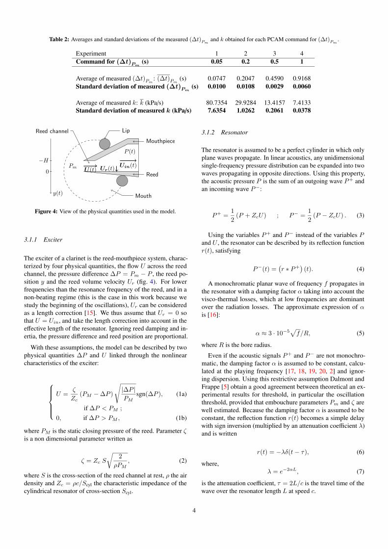
Table 2: Averages and standard deviations of the measured (∆t)Pmand k obtained for each PCAM command for (∆t)Pm

.

Experiment 1 2 3 4Command for (∆t)Pm

(s) 0.05 0.2 0.5 1

Average of measured (∆t)Pm: (∆t)Pm

(s) 0.0747 0.2047 0.4590 0.9168Standard deviation of measured (∆t)Pm

(s) 0.0100 0.0108 0.0029 0.0060

Average of measured k: k (kPa/s) 80.7354 29.9284 13.4157 7.4133Standard deviation of measured k (kPa/s) 7.6354 1.0262 0.2061 0.0378

y(t)

−H

0 U(t) Ur(t)Uin(t)

P (t)

Mouthpiece

Reed

Lip

Mouth

Pm

Reed channel

Figure 4: View of the physical quantities used in the model.

3.1.1 Exciter

The exciter of a clarinet is the reed-mouthpiece system, charac-terized by four physical quantities, the flow U across the reedchannel, the pressure difference ∆P = Pm − P , the reed po-sition y and the reed volume velocity Ur (fig. 4). For lowerfrequencies than the resonance frequency of the reed, and in anon-beating regime (this is the case in this work because westudy the beginning of the oscillations), Ur can be consideredas a length correction [15]. We thus assume that Ur = 0 sothat U = Uin, and take the length correction into account in theeffective length of the resonator. Ignoring reed damping and in-ertia, the pressure difference and reed position are proportional.

With these assumptions, the model can be described by twophysical quantities ∆P and U linked through the nonlinearcharacteristics of the exciter:

U =ζ

Zc(PM −∆P )

√|∆P |PM

sgn(∆P ), (1a)

if ∆P < PM ;

0, if ∆P > PM , (1b)

where PM is the static closing pressure of the reed. Parameter ζis a non dimensional parameter written as

ζ = Zc S

√2

ρPM, (2)

where S is the cross-section of the reed channel at rest, ρ the airdensity and Zc = ρc/Scyl the characteristic impedance of thecylindrical resonator of cross-section Scyl.

3.1.2 Resonator

The resonator is assumed to be a perfect cylinder in which onlyplane waves propagate. In linear acoustics, any unidimensionalsingle-frequency pressure distribution can be expanded into twowaves propagating in opposite directions. Using this property,the acoustic pressure P is the sum of an outgoing wave P+ andan incoming wave P−:

P+ =1

2(P + ZcU) ; P− =

1

2(P − ZcU) . (3)

Using the variables P+ and P− instead of the variables Pand U , the resonator can be described by its reflection functionr(t), satisfying

P−(t) =(r ∗ P+

)(t). (4)

A monochromatic planar wave of frequency f propagates inthe resonator with a damping factor α taking into account thevisco-thermal losses, which at low frequencies are dominantover the radiation losses. The approximate expression of αis [16]:

α ≈ 3 · 10−5√f/R, (5)

where R is the bore radius.

Even if the acoustic signals P+ and P− are not monochro-matic, the damping factor α is assumed to be constant, calcu-lated at the playing frequency [17, 18, 19, 20, 2] and ignor-ing dispersion. Using this restrictive assumption Dalmont andFrappe [5] obtain a good agreement between theoretical an ex-perimental results for threshold, in particular the oscillationthreshold, provided that embouchure parameters Pm and ζ arewell estimated. Because the damping factor α is assumed to beconstant, the reflection function r(t) becomes a simple delaywith sign inversion (multiplied by an attenuation coefficient λ)and is written

r(t) = −λδ(t− τ), (6)

where,λ = e−2αL, (7)

is the attenuation coefficient, τ = 2L/c is the travel time of thewave over the resonator length L at speed c.

4

-4 -2 0 2 4

-4

-2

0

2

4

−P− (kPa)

P+=

G(−

P−)

(kPa)

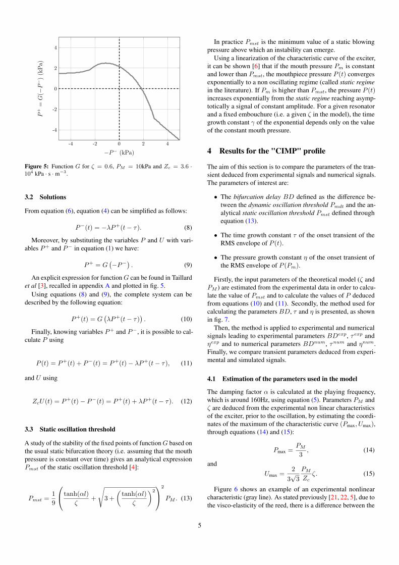
Figure 5: Function G for ζ = 0.6, PM = 10kPa and Zc = 3.6 ·104 kPa · s · m−3.

3.2 Solutions

From equation (6), equation (4) can be simplified as follows:

P−(t) = −λP+(t− τ). (8)

Moreover, by substituting the variables P and U with vari-ables P+ and P− in equation (1) we have:

P+ = G(−P−

). (9)

An explicit expression for functionG can be found in Taillardet al [3], recalled in appendix A and plotted in fig. 5.

Using equations (8) and (9), the complete system can bedescribed by the following equation:

P+(t) = G(λP+(t− τ)

). (10)

Finally, knowing variables P+ and P−, it is possible to cal-culate P using

P (t) = P+(t) + P−(t) = P+(t)− λP+(t− τ), (11)

and U using

ZcU(t) = P+(t)− P−(t) = P+(t) + λP+(t− τ). (12)

3.3 Static oscillation threshold

A study of the stability of the fixed points of functionG based onthe usual static bifurcation theory (i.e. assuming that the mouthpressure is constant over time) gives an analytical expressionPmst of the static oscillation threshold [4]:

Pmst =1

9

tanh(αl)

ζ+

√3 +

(tanh(αl)

ζ

)2

2

PM . (13)

In practice Pmst is the minimum value of a static blowingpressure above which an instability can emerge.

Using a linearization of the characteristic curve of the exciter,it can be shown [6] that if the mouth pressure Pm is constantand lower than Pmst, the mouthpiece pressure P (t) convergesexponentially to a non oscillating regime (called static regimein the literature). If Pm is higher than Pmst, the pressure P (t)increases exponentially from the static regime reaching asymp-totically a signal of constant amplitude. For a given resonatorand a fixed embouchure (i.e. a given ζ in the model), the timegrowth constant γ of the exponential depends only on the valueof the constant mouth pressure.

4 Results for the "CIMP" profile

The aim of this section is to compare the parameters of the tran-sient deduced from experimental signals and numerical signals.The parameters of interest are:

• The bifurcation delay BD defined as the difference be-tween the dynamic oscillation threshold Pmdt and the an-alytical static oscillation threshold Pmst defined throughequation (13).

• The time growth constant τ of the onset transient of theRMS envelope of P (t).

• The pressure growth constant η of the onset transient ofthe RMS envelope of P (Pm).

Firstly, the input parameters of the theoretical model (ζ andPM ) are estimated from the experimental data in order to calcu-late the value of Pmst and to calculate the values of P deducedfrom equations (10) and (11). Secondly, the method used forcalculating the parameters BD, τ and η is presented, as shownin fig. 7.

Then, the method is applied to experimental and numericalsignals leading to experimental parameters BDexp, τexp andηexp and to numerical parameters BDnum, τnum and ηnum.Finally, we compare transient parameters deduced from experi-mental and simulated signals.

4.1 Estimation of the parameters used in the model

The damping factor α is calculated at the playing frequency,which is around 160Hz, using equation (5). Parameters PM andζ are deduced from the experimental non linear characteristicsof the exciter, prior to the oscillation, by estimating the coordi-nates of the maximum of the characteristic curve (Pmax, Umax),through equations (14) and (15):

Pmax =PM3, (14)

andUmax =

2

3√

3

PMZc

ζ. (15)

Figure 6 shows an example of an experimental nonlinearcharacteristic (gray line). As stated previously [21, 22, 5], due tothe visco-elasticity of the reed, there is a difference between the

5

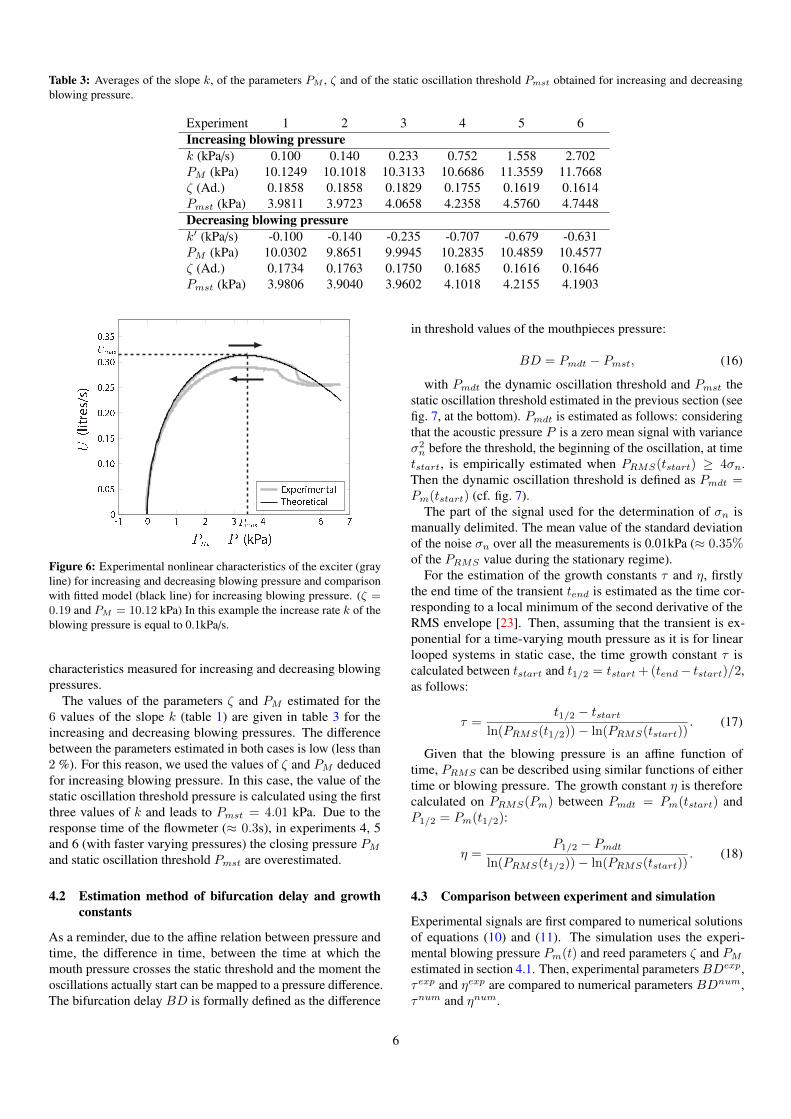
Table 3: Averages of the slope k, of the parameters PM , ζ and of the static oscillation threshold Pmst obtained for increasing and decreasingblowing pressure.

Experiment 1 2 3 4 5 6Increasing blowing pressurek (kPa/s) 0.100 0.140 0.233 0.752 1.558 2.702PM (kPa) 10.1249 10.1018 10.3133 10.6686 11.3559 11.7668ζ (Ad.) 0.1858 0.1858 0.1829 0.1755 0.1619 0.1614Pmst (kPa) 3.9811 3.9723 4.0658 4.2358 4.5760 4.7448Decreasing blowing pressurek′ (kPa/s) -0.100 -0.140 -0.235 -0.707 -0.679 -0.631PM (kPa) 10.0302 9.8651 9.9945 10.2835 10.4859 10.4577ζ (Ad.) 0.1734 0.1763 0.1750 0.1685 0.1616 0.1646Pmst (kPa) 3.9806 3.9040 3.9602 4.1018 4.2155 4.1903

-� 0 � 2 3�m�� 44 6 70

0�0�

0��0

0���

0�20

0�2�

0�30�m��

0�3�

�� � � (�Pa�

�� ������

E�pe���ent��T�e��et����

Figure 6: Experimental nonlinear characteristics of the exciter (grayline) for increasing and decreasing blowing pressure and comparisonwith fitted model (black line) for increasing blowing pressure. (ζ =0.19 and PM = 10.12 kPa) In this example the increase rate k of theblowing pressure is equal to 0.1kPa/s.

characteristics measured for increasing and decreasing blowingpressures.

The values of the parameters ζ and PM estimated for the6 values of the slope k (table 1) are given in table 3 for theincreasing and decreasing blowing pressures. The differencebetween the parameters estimated in both cases is low (less than2 %). For this reason, we used the values of ζ and PM deducedfor increasing blowing pressure. In this case, the value of thestatic oscillation threshold pressure is calculated using the firstthree values of k and leads to Pmst = 4.01 kPa. Due to theresponse time of the flowmeter (≈ 0.3s), in experiments 4, 5and 6 (with faster varying pressures) the closing pressure PMand static oscillation threshold Pmst are overestimated.

4.2 Estimation method of bifurcation delay and growthconstants

As a reminder, due to the affine relation between pressure andtime, the difference in time, between the time at which themouth pressure crosses the static threshold and the moment theoscillations actually start can be mapped to a pressure difference.The bifurcation delay BD is formally defined as the difference

in threshold values of the mouthpieces pressure:

BD = Pmdt − Pmst, (16)

with Pmdt the dynamic oscillation threshold and Pmst thestatic oscillation threshold estimated in the previous section (seefig. 7, at the bottom). Pmdt is estimated as follows: consideringthat the acoustic pressure P is a zero mean signal with varianceσ2n before the threshold, the beginning of the oscillation, at timetstart, is empirically estimated when PRMS(tstart) ≥ 4σn.Then the dynamic oscillation threshold is defined as Pmdt =Pm(tstart) (cf. fig. 7).

The part of the signal used for the determination of σn ismanually delimited. The mean value of the standard deviationof the noise σn over all the measurements is 0.01kPa (≈ 0.35%of the PRMS value during the stationary regime).

For the estimation of the growth constants τ and η, firstlythe end time of the transient tend is estimated as the time cor-responding to a local minimum of the second derivative of theRMS envelope [23]. Then, assuming that the transient is ex-ponential for a time-varying mouth pressure as it is for linearlooped systems in static case, the time growth constant τ iscalculated between tstart and t1/2 = tstart + (tend− tstart)/2,as follows:

τ =t1/2 − tstart

ln(PRMS(t1/2))− ln(PRMS(tstart)). (17)

Given that the blowing pressure is an affine function oftime, PRMS can be described using similar functions of eithertime or blowing pressure. The growth constant η is thereforecalculated on PRMS(Pm) between Pmdt = Pm(tstart) andP1/2 = Pm(t1/2):

η =P1/2 − Pmdt

ln(PRMS(t1/2))− ln(PRMS(tstart)). (18)

4.3 Comparison between experiment and simulation

Experimental signals are first compared to numerical solutionsof equations (10) and (11). The simulation uses the experi-mental blowing pressure Pm(t) and reed parameters ζ and PMestimated in section 4.1. Then, experimental parametersBDexp,τexp and ηexp are compared to numerical parameters BDnum,τnum and ηnum.

6

3 3�� Pm�� 4�� � ��� 6 6�� 70

1

2

�

�

5

�

�

� (�a)

�RMS ����

k�k�k�k�k�k�

(a) Experiment

3.5 Pmst 4.5 5 5.5 6 6.5 70

1

2

3

4

5

6

7

Pm (kPa)

PRM

S(k

Pa)

k6k5k4k3k2k1

(b) Simulation

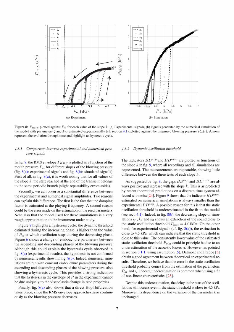
Figure 8: PRMS plotted against Pm for each value of the slope k. (a) Experimental signals, (b) signals generated by the numerical simulation ofthe model with parameters ζ and PM estimated experimentally (cf. section 4.1), plotted against the measured blowing pressure Pm(t). Arrowsrepresent the evolution through time and highlight an hysteretis cycle.

4.3.1 Comparison between experimental and numerical pres-sure signals

In fig. 8, the RMS envelope PRMS is plotted as a function of themouth pressure Pm for different slopes of the blowing pressure(fig. 8(a): experimental signals and fig. 8(b): simulated signals).First of all, in fig. 8(a), it is worth noting that for all values ofthe slope k, the state reached at the end of the transient belongsto the same periodic branch (slight repeatability errors aside).

Secondly, we can observe a substantial difference betweenthe experimental and numerical signal amplitudes. Two reasonscan explain this difference. The first is the fact that the dampingfactor is estimated at the playing frequency. A second reasoncould be the error made on the estimation of the reed parameters.Note also that the model used for these simulations is a veryrough approximation to the instrument under study.

Figure 8 highlights a hysteresis cycle: the dynamic thresholdestimated during the increasing phase is higher than the valueof Pm at which oscillation stops during the decreasing phase.Figure 6 shows a change of embouchure parameters betweenthe ascending and descending phases of the blowing pressure.Although this could explain the hysteresis cycle observed infig. 8(a) (experimental results), the hypothesis is not confirmedby numerical results shown in fig. 8(b). Indeed, numerical simu-lations are run with constant embouchure parameters during theascending and descending phases of the blowing pressure, alsoshowing a hysteresis cycle. This provides a strong indicationthat the hysteresis in the envelope of P in the experiment cannotbe due uniquely to the viscoelastic change in reed properties.

Finally, fig. 8(a) also shows that a direct Hopf bifurcationtakes place, since the RMS envelope approaches zero continu-ously as the blowing pressure decreases.

4.3.2 Dynamic oscillation threshold

The indicators BDexp and BDnum are plotted as functions ofthe slope k in fig. 9, where all recordings and all simulations arerepresented. The measurements are repeatable, showing littledifference between the three tests of each slope k.

As suggested by fig. 8, the gaps BDexp and BDnum are al-ways positive and increase with the slope k. This is as predictedby recent theoretical predictions on a discrete time system af-fected with noise[24]. Figure 9 shows that the indicatorBDnum

estimated on numerical simulations is always smaller than theexperimentalBDexp. A possible reason for this is that the staticoscillation threshold is underestimated in the fit to the model(see sect. 4.1). Indeed, in fig. 8(b), the decreasing slope of simu-lations k1, k2 and k3 shows an extinction of the sound close tothe static oscillation threshold Pmst = 4.01kPa. On the otherhand, for experimental signals (cf. fig. 8(a)), the extinction isclose to 4.5 kPa, which can indicate that the static threshold isclose to this value. The consistently lower value of the estimatedstatic oscillation threshold Pmst could in principle be due to anunderestimation of the acoustic losses α. However, as pointedin section 3.1.1, using assumption (5), Dalmont and Frappe [5]obtain a good agreement between theoretical an experimental re-sults. Therefore, we believe that the error in the static oscillationthreshold probably comes from the estimation of the parametersPM and ζ . Indeed, underestimation is common when using a fitof non-linear characteristics [25].

Despite this underestimation, the delay in the start of the oscil-lations still occurs even if the static threshold is close to 4.5 kPa.Moreover, its dependence on the variation of the parameter k isunchanged.

7

Onsettransient

Time

Pre

ssur

e

•

•

σn

4σn

Pmdt

P1/2

Pend

tstartt1/2

tend

∼ exp(tτ

)

Pm

PRMS

Onsettransient

Mouth pressure

Pre

ssur

e(P

RM

S)

•

•

•

Pmdt P1/2 Pend

∼ exp(

Pm

η

)

Onsettransient

Mouth pressure

Pre

ssur

e(P

RM

S)

•

Bifurcationdelay(BD)

Pmst Pmdt

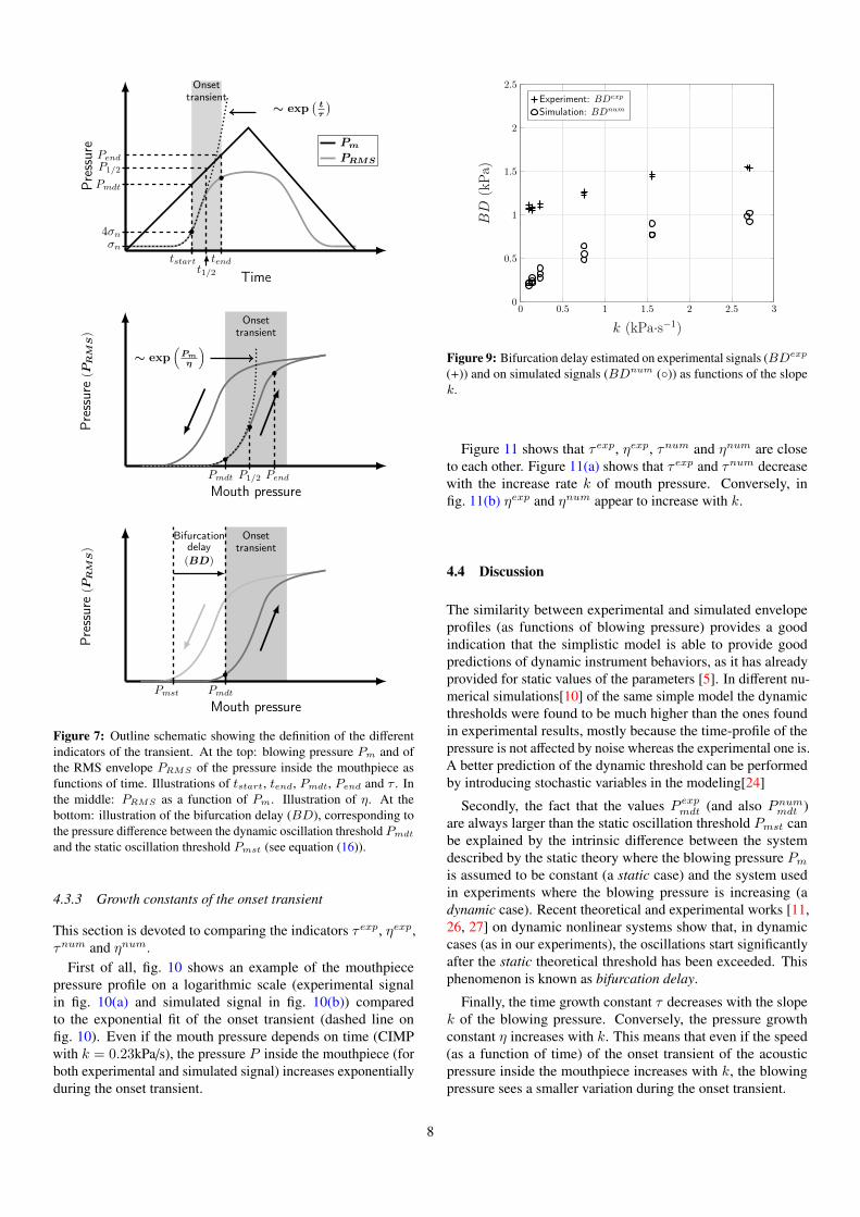
Figure 7: Outline schematic showing the definition of the differentindicators of the transient. At the top: blowing pressure Pm and ofthe RMS envelope PRMS of the pressure inside the mouthpiece asfunctions of time. Illustrations of tstart, tend, Pmdt, Pend and τ . Inthe middle: PRMS as a function of Pm. Illustration of η. At thebottom: illustration of the bifurcation delay (BD), corresponding tothe pressure difference between the dynamic oscillation threshold Pmdt

and the static oscillation threshold Pmst (see equation (16)).

4.3.3 Growth constants of the onset transient

This section is devoted to comparing the indicators τexp, ηexp,τnum and ηnum.

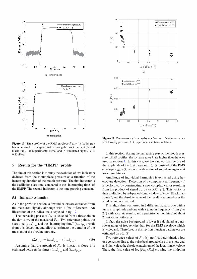
First of all, fig. 10 shows an example of the mouthpiecepressure profile on a logarithmic scale (experimental signalin fig. 10(a) and simulated signal in fig. 10(b)) comparedto the exponential fit of the onset transient (dashed line onfig. 10). Even if the mouth pressure depends on time (CIMPwith k = 0.23kPa/s), the pressure P inside the mouthpiece (forboth experimental and simulated signal) increases exponentiallyduring the onset transient.

0 0.5 1 1.5 2 2.5 30

0.5

1

1.5

2

2.5

k (kPa·s−1)

BD

(kPa

)

Experiment: BDexp

Simulation: BDnum

Figure 9: Bifurcation delay estimated on experimental signals (BDexp

(+)) and on simulated signals (BDnum (◦)) as functions of the slopek.

Figure 11 shows that τexp, ηexp, τnum and ηnum are closeto each other. Figure 11(a) shows that τexp and τnum decreasewith the increase rate k of mouth pressure. Conversely, infig. 11(b) ηexp and ηnum appear to increase with k.

4.4 Discussion

The similarity between experimental and simulated envelopeprofiles (as functions of blowing pressure) provides a goodindication that the simplistic model is able to provide goodpredictions of dynamic instrument behaviors, as it has alreadyprovided for static values of the parameters [5]. In different nu-merical simulations[10] of the same simple model the dynamicthresholds were found to be much higher than the ones foundin experimental results, mostly because the time-profile of thepressure is not affected by noise whereas the experimental one is.A better prediction of the dynamic threshold can be performedby introducing stochastic variables in the modeling[24]

Secondly, the fact that the values P expmdt (and also Pnummdt )are always larger than the static oscillation threshold Pmst canbe explained by the intrinsic difference between the systemdescribed by the static theory where the blowing pressure Pmis assumed to be constant (a static case) and the system usedin experiments where the blowing pressure is increasing (adynamic case). Recent theoretical and experimental works [11,26, 27] on dynamic nonlinear systems show that, in dynamiccases (as in our experiments), the oscillations start significantlyafter the static theoretical threshold has been exceeded. Thisphenomenon is known as bifurcation delay.

Finally, the time growth constant τ decreases with the slopek of the blowing pressure. Conversely, the pressure growthconstant η increases with k. This means that even if the speed(as a function of time) of the onset transient of the acousticpressure inside the mouthpiece increases with k, the blowingpressure sees a smaller variation during the onset transient.

8

(a) Experiment

(b) Simulation

Figure 10: Time profile of the RMS envelope PRMS(t) (solid grayline) compared to its exponential fit during the onset transient (dashedblack line). (a) Experimental signal and (b) simulated signal. k =0.23kPa/s.

5 Results for the "IIMPP" profile

The aim of this section is to study the evolution of two indicatorsdeduced from the mouthpiece pressure as a function of theincreasing duration of the mouth pressure. The first indicator isthe oscillation start time, compared to the “interrupting time” ofthe IIMPP. The second indicator is the time growing constant.

5.1 Indicator estimation

As in the previous section, a few indicators are extracted fromthe measured signals, although with a few differences. Anillustration of the indicators is depicted in fig. 12.

The increasing phase of Pm is detected from a threshold onthe derivative of the measured Pm. Two reference points, thestart time (tstart)Pm

and the “interrupting time” (tend)Pm, result

from this detection, and allow to estimate the duration of thetransient of the blowing pressure:

(∆t)Pm= (tend)Pm

− (tstart)Pm. (19)

Assuming that the growth of Pm is linear, its slope k isestimated between the times (tstart)Pm

and (tend)Pm.

0 0.5 1 1.5 2 2.5 300

0.1

0.2

0.3

k (kPa·s−1)

τ(s

)

Experiment: τexp

Simulation: τnum

(a)

0 0.5 1 1.5 2 2.5 30

0.04

0.08

0.12

0.16

k (kPa·s−1)

η(P

a)

Experiment: ηexp

Simulation: ηnum

(b)

Figure 11: Parameters τ (a) and η (b) as a function of the increase ratek of blowing pressure. (+) Experiment and (◦) simulation.

In this section, during the increasing part of the mouth pres-sure IIMPP profiles, the increase rates k are higher than the onesused in section 4. In this case, we have noted that the use ofthe amplitude of the first harmonic PH1

(t) instead of the RMSenvelope PRMS(t) allows the detection of sound emergence atlower amplitudes.

Amplitude of individual harmonics is extracted using het-erodyne detection. Detection of a component at frequency fis performed by constructing a new complex vector resultingfrom the product of signal xn by exp(j2πft). This vector isthen multiplied by a 4-period-long window of type “Blackman-Harris”, and the absolute value of the result is summed over thewindow and normalized.

This algorithm was tested in 2 different signals: one with ajump in amplitude and one with a jump in frequency (from f to2f ) with accurate results, and a precision (smoothing) of about2 periods in both cases.

In fact, the noise background is lower if calculated at a nar-rower range of frequencies than for the RMS envelope whichis wideband. Therefore, in this section transient parameters areestimated on PH1

(t).Two reference values of PH1

(t) are first determined, a lowone corresponding to the noise background close to the note end,and high value, the absolute maximum of the logarithm envelope.Then, the first value of log [PH1/Pref] crossing the midpoint

9

(∆ t)Pm

(∆ t)P H1

T

t10

t30

t50

t70t90

Time

log[P

H1(t)/Pref]

dPm(t)/dt

Pm(t)

(tstart )Pm“Interrupting time”(tend)Pm

≡

(a)

(b)

(c)

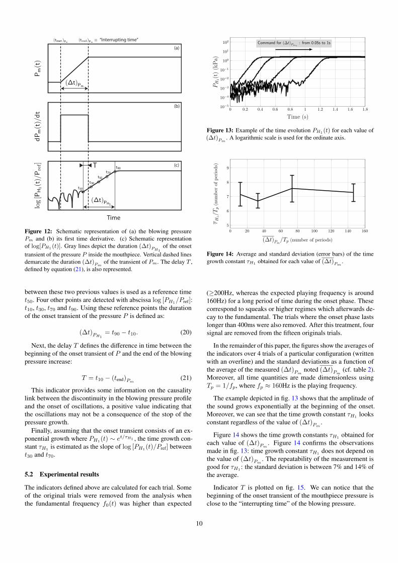
Figure 12: Schematic representation of (a) the blowing pressurePm and (b) its first time derivative. (c) Schematic representationof log[PH1(t)]. Gray lines depict the duration (∆t)PH1

of the onsettransient of the pressure P inside the mouthpiece. Vertical dashed linesdemarcate the duration (∆t)Pm

of the transient of Pm. The delay T ,defined by equation (21), is also represented.

between these two previous values is used as a reference timet50. Four other points are detected with abscissa log [PH1

/Pref]:t10, t30, t70 and t90. Using these reference points the durationof the onset transient of the pressure P is defined as:

(∆t)PH1= t90 − t10. (20)

Next, the delay T defines the difference in time between thebeginning of the onset transient of P and the end of the blowingpressure increase:

T = t10 − (tend)Pm(21)

This indicator provides some information on the causalitylink between the discontinuity in the blowing pressure profileand the onset of oscillations, a positive value indicating thatthe oscillations may not be a consequence of the stop of thepressure growth.

Finally, assuming that the onset transient consists of an ex-ponential growth where PH1(t) ∼ et/τH1 , the time growth con-stant τH1 is estimated as the slope of log [PH1(t)/Pref] betweent30 and t70.

5.2 Experimental results

The indicators defined above are calculated for each trial. Someof the original trials were removed from the analysis whenthe fundamental frequency f0(t) was higher than expected

0 0.2 0.4 0.6 0.8 1 1.2 1.4 1.6 1.810−5

10−4

10−3

10−2

10−1

100

101

102 Command for (∆t)Pms: from 0.05s to 1s

Time (s)

PH

1(t

)(k

Pa)

Figure 13: Example of the time evolution PH1(t) for each value of(∆t)Pm

. A logarithmic scale is used for the ordinate axis.

0 20 40 60 80 100 120 140 160

5

6

7

8

9

(∆t)Pm/Tp (number of periods)

τH

1/T

p(n

umbe

rof

peri

ods)

Figure 14: Average and standard deviation (error bars) of the timegrowth constant τH1 obtained for each value of (∆t)Pm

.

(≥200Hz, whereas the expected playing frequency is around160Hz) for a long period of time during the onset phase. Thesecorrespond to squeaks or higher regimes which afterwards de-cay to the fundamental. The trials where the onset phase lastslonger than 400ms were also removed. After this treatment, foursignal are removed from the fifteen originals trials.

In the remainder of this paper, the figures show the averages ofthe indicators over 4 trials of a particular configuration (writtenwith an overline) and the standard deviations as a function ofthe average of the measured (∆t)Pm

noted (∆t)Pm(cf. table 2).

Moreover, all time quantities are made dimensionless usingTp = 1/fp, where fp ≈ 160Hz is the playing frequency.

The example depicted in fig. 13 shows that the amplitude ofthe sound grows exponentially at the beginning of the onset.Moreover, we can see that the time growth constant τH1

looksconstant regardless of the value of (∆t)Pm

.

Figure 14 shows the time growth constants τH1obtained for

each value of (∆t)Pm. Figure 14 confirms the observations

made in fig. 13: time growth constant τH1 does not depend onthe value of (∆t)Pm

. The repeatability of the measurement isgood for τH1

: the standard deviation is between 7% and 14% ofthe average.

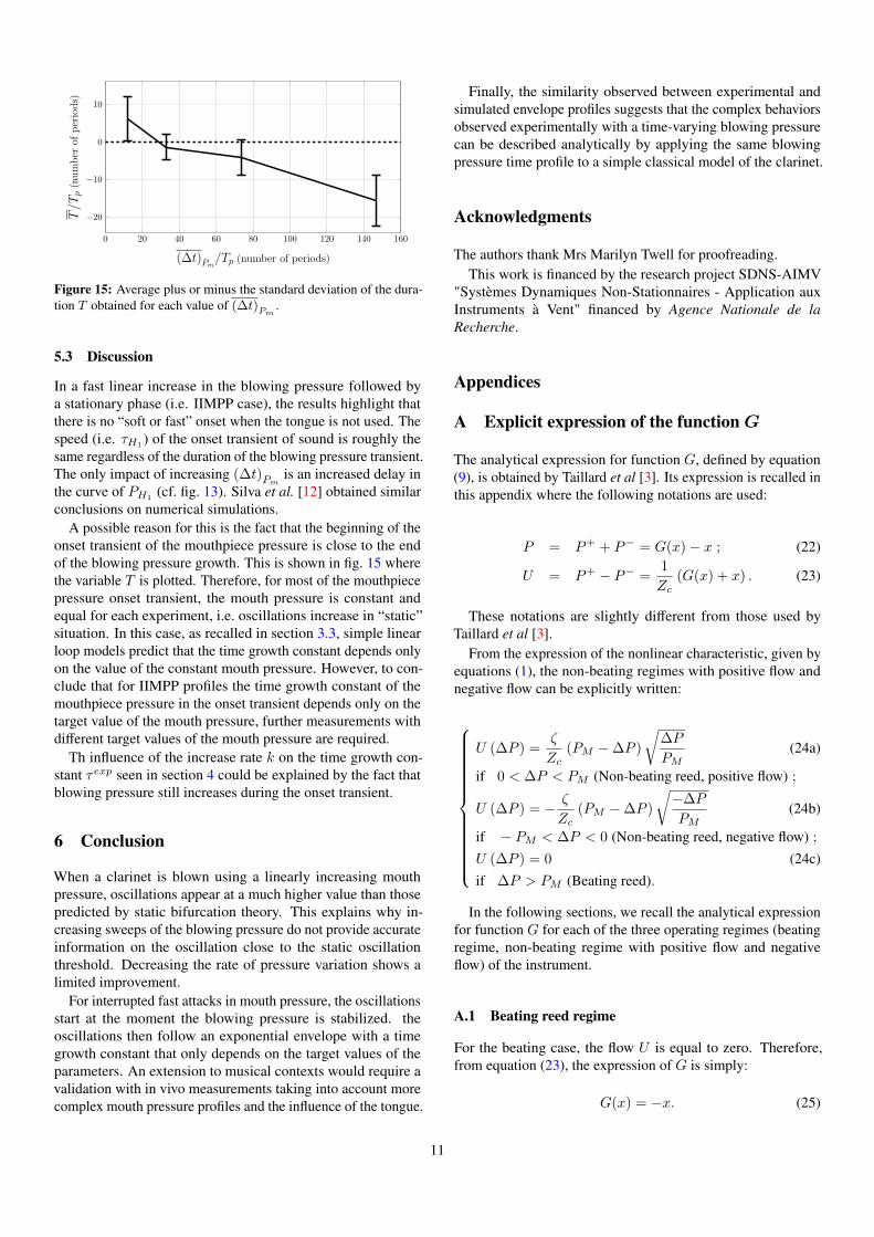
Indicator T is plotted on fig. 15. We can notice that thebeginning of the onset transient of the mouthpiece pressure isclose to the “interrupting time” of the blowing pressure.

10

0 20 40 60 80 100 120 140 160

−20

−10

0

10

(∆t)Pm/Tp (number of periods)

T/T

p(n

umbe

rof

peri

ods)

Figure 15: Average plus or minus the standard deviation of the dura-tion T obtained for each value of (∆t)Pm

.

5.3 Discussion

In a fast linear increase in the blowing pressure followed bya stationary phase (i.e. IIMPP case), the results highlight thatthere is no “soft or fast” onset when the tongue is not used. Thespeed (i.e. τH1

) of the onset transient of sound is roughly thesame regardless of the duration of the blowing pressure transient.The only impact of increasing (∆t)Pm

is an increased delay inthe curve of PH1 (cf. fig. 13). Silva et al. [12] obtained similarconclusions on numerical simulations.

A possible reason for this is the fact that the beginning of theonset transient of the mouthpiece pressure is close to the endof the blowing pressure growth. This is shown in fig. 15 wherethe variable T is plotted. Therefore, for most of the mouthpiecepressure onset transient, the mouth pressure is constant andequal for each experiment, i.e. oscillations increase in “static”situation. In this case, as recalled in section 3.3, simple linearloop models predict that the time growth constant depends onlyon the value of the constant mouth pressure. However, to con-clude that for IIMPP profiles the time growth constant of themouthpiece pressure in the onset transient depends only on thetarget value of the mouth pressure, further measurements withdifferent target values of the mouth pressure are required.

Th influence of the increase rate k on the time growth con-stant τexp seen in section 4 could be explained by the fact thatblowing pressure still increases during the onset transient.

6 Conclusion

When a clarinet is blown using a linearly increasing mouthpressure, oscillations appear at a much higher value than thosepredicted by static bifurcation theory. This explains why in-creasing sweeps of the blowing pressure do not provide accurateinformation on the oscillation close to the static oscillationthreshold. Decreasing the rate of pressure variation shows alimited improvement.

For interrupted fast attacks in mouth pressure, the oscillationsstart at the moment the blowing pressure is stabilized. theoscillations then follow an exponential envelope with a timegrowth constant that only depends on the target values of theparameters. An extension to musical contexts would require avalidation with in vivo measurements taking into account morecomplex mouth pressure profiles and the influence of the tongue.

Finally, the similarity observed between experimental andsimulated envelope profiles suggests that the complex behaviorsobserved experimentally with a time-varying blowing pressurecan be described analytically by applying the same blowingpressure time profile to a simple classical model of the clarinet.

Acknowledgments

The authors thank Mrs Marilyn Twell for proofreading.This work is financed by the research project SDNS-AIMV

"Systèmes Dynamiques Non-Stationnaires - Application auxInstruments à Vent" financed by Agence Nationale de laRecherche.

Appendices

A Explicit expression of the function G

The analytical expression for function G, defined by equation(9), is obtained by Taillard et al [3]. Its expression is recalled inthis appendix where the following notations are used:

P = P+ + P− = G(x)− x ; (22)

U = P+ − P− =1

Zc(G(x) + x) . (23)

These notations are slightly different from those used byTaillard et al [3].

From the expression of the nonlinear characteristic, given byequations (1), the non-beating regimes with positive flow andnegative flow can be explicitly written:

U (∆P ) =ζ

Zc(PM −∆P )

√∆P

PM(24a)

if 0 < ∆P < PM (Non-beating reed, positive flow) ;

U (∆P ) = − ζ

Zc(PM −∆P )

√−∆P

PM(24b)

if − PM < ∆P < 0 (Non-beating reed, negative flow) ;

U (∆P ) = 0 (24c)if ∆P > PM (Beating reed).

In the following sections, we recall the analytical expressionfor function G for each of the three operating regimes (beatingregime, non-beating regime with positive flow and negativeflow) of the instrument.

A.1 Beating reed regime

For the beating case, the flow U is equal to zero. Therefore,from equation (23), the expression of G is simply:

G(x) = −x. (25)

11

A.2 Non-beating reed regimes

From equation (22) and recalling that ∆P = Pm − P , functionG can be written as follow:

G(x) = Pm + ∆P (U) + x. (26)

Therefore, inverting equations (24b) and (24c) leads to adirect analytical expression of function G for the positive andnegative flow cases respectively. In practice, inverting (24b) and(24c) consists in solving a third order polynomial equation, asexplained by Taillard et al [3].

A.2.1 Positive flow

For the non-beating reed regime with positive flow, the analyti-cal expression for function G is:

G(x) = Pm − PM(−2

3η×

sin

1

3arcsin

ψ − 9

2

(3PM

(Pm + 2x)− 1)

ζη3

+

1

3ζ

2

+ x, (27)

with,

ψ =1

ζ2; η =

√3 + ψ. (28)

A.2.2 Negative flow

As stated above, inverting equation (24c) consists in solvinga third order polynomial equation. For the non-beating reedregime with negative flow, the analytical expression of functionG depends on the sign of the discriminant of the polynomial:

Discr = q3 + r2, (29)

with

q =1

9(3− ψ) ; r = −

ψ + 92

(3PM

(Pm + 2x)− 1)

27ζ.

(30)

Positive discriminant. In this case, the expression of G is:

G(x) = Pm + PM

(s1 −

q

s1− 1

3ζ

)2

+ x, (31)

where,

s1 =[r +√

Discr]1/3

. (32)

Negative discriminant. G is:

G(x) = Pm + PM

(2

3η′×

cos

1

3arccos

−ψ − 9

2

(3PM

(Pm + 2x)− 1)

ζη′3

− 1

3ζ

2

+ x, (33)

with,

η′ =√−3 + ψ. (34)

References

[1] V. Debut and J. Kergomard, “Analysis of the self-sustainedoscillations of a clarinet as a van der pol oscillator”, in18th International Congress on Acoustics-ICA, volume 2,1425–1428 (2004).

[2] J. P. Dalmont, J. Gilbert, J. Kergomard, and S. Ollivier,“An analytical prediction of the oscillation and extinctionthresholds of a clarinet”, J. Acoust. Soc. Am. 118, 3294–3305 (2005).

[3] P. Taillard, J. Kergomard, and F. Laloë, “Iterated mapsfor clarinet-like systems”, Nonlinear Dynam. 62, 253–271(2010).

[4] J. Kergomard, S. Ollivier, and J. Gilbert, “Calculationof the spectrum of self-sustained oscillators using a vari-able troncation method”, Acta. Acust. Acust. 86, 665–703(2000).

[5] J. P. Dalmont and C. Frappe, “Oscillation and extinctionthresholds of the clarinet: Comparison of analytical resultsand experiments”, J. Acoust. Soc. Am. 122, 1173–1179(2007).

[6] A. Chaigne and J. Kergomard, “Instruments à anche (reedinstruments)”, in Acoustique des instruments de musique(Acoustics of musical instruments), chapter 9, 400–468(Belin) (2008).

[7] S. Karkar, C. Vergez, and B. Cochelin, “Oscillation thresh-old of a clarinet model: A numerical continuation ap-proach”, The Journal of the Acoustical Society of America131, 698–707 (2012).

[8] B. Gazengel and J. P. Dalmont, “Mechanical response char-acterization of saxophone reeds”, in 6th Forum Acusticum(Aalborg, Denmark, 26 June-1 July 2011).

[9] M. Atig, J. P. Dalmont, and J. Gilbert, “Saturation mecha-nism in clarinet-like instruments, the effect of the localisednonlinear losses”, Appl. Acoust. 65, 1133–1154 (2004).

12

[10] B. Bergeot, C. Vergez, A. Almeida, and B. Gazengel,“Prediction of the dynamic oscillation threshold in a clar-inet model with a linearly increasing blowing pressure”,Nonlinear Dynam. 73, 521–534 (2013), URL http://dx.doi.org/10.1007/s11071-013-0806-y (date lastviewed 5/28/13).

[11] A. Fruchard and R. Schäfke, “Sur le retard à la bifurcation(on the bifurcation delay)”, Arima 9, 431–468 (2008).

[12] F. Silva, P. Guillemain, J. Kergomard, C. Vergez, andV. Debut, “Some simulations of the effect of varying ex-citation parameters on the transients of reed instruments”,(2013-01), URL http://hal.archives-ouvertes.fr/hal-00779636 (date last viewed 5/28/13).

[13] D. Ferrand and C. Vergez, “Blowing machine for windmusical instrument : toward a real-time control of blowingpressure”, in 16th IEEE Mediterranean Conference onControl and Automation (MED), 1562–1567 (Ajaccion,France) (2008).

[14] D. Ferrand, C. Vergez, B. Fabre, and F. Blanc, “High-precision regulation of a pressure controlled artificialmouth : the case of recorder-like musical instruments”,Acta. Acust. Acust. 96, 701–712 (2010).

[15] C. J. Nederveen, Acoustical aspects of woodwind instru-ments (Northern Illinois University Press, Illinois) 28–35(Revised edition, 1998).

[16] D. H. Keefe, “Acoustical wave propagation in cylindricalducts: transmission line parameter approximations forisothermal and non-isothermal boundary conditions”, J.Acoust. Soc. Am. 75, 58–62 (1984).

[17] C. Maganza, R. Caussé, and F. Laloë, “Bifurcations, pe-riod doublings and chaos in clarinet-like systems”, EPL(Europhysics Letters) 1, 295 (1986).

[18] J. Kergomard, “Elementary considerations on reed-instrument oscillations”, in Mechanics of musical instru-ments by A. Hirschberg/ J. Kergomard/ G. Weinreich, vol-ume 335 of CISM Courses and lectures, chapter 6, 229–290 (Springer-Verlag) (1995).

[19] J. Kergomard, J. P. Dalmont, J. Gilbert, and P. Guillemain,“Period doubling on cylindrical reed instruments”, in Pro-ceeding of the Joint congress CFA/DAGA 04, 113–114(Société Française d’Acoustique - Deutsche Gesellschaftfür Akustik) (2004, Strasbourg, France).

[20] S. Ollivier, J. P. Dalmont, and J. Kergomard, “Idealizedmodels of reed woodwinds. part 2 : On the stability of two-step oscillations”, Acta. Acust. united Ac. 91, 166–179(2005).

[21] J. P. Dalmont, J. Gilbert, and S. Ollivier, “Nonlinear char-acteristics of single-reed instruments: Quasistatic volumeflow and reed opening measurements”, J. Acoust. Soc. Am.114, 2253–2262 (2003).

[22] A. Almeida, C. Vergez, and R. Caussé, “Quasi-staticnonlinear characteristics of double-reed instruments”, J.Acoust. Soc. Am. 121, 536–546 (2007).

[23] K. Jensen, “Enveloppe model of isolated musical sounds”,Proceedings of the 2nd COST G-6 Workshop on DigitalAudio Effects (DAFx99), NTNU, Trondheim (1999).

[24] B. Bergeot, C. Vergez, A. Almeida, and B. Gazen-gel, “Prediction of the dynamic oscillation thresholdin a clarinet model with a linearly increasing blowingpressure: Influence of noise”, Nonlinear Dynam. 74,591–605 (2013), URL http://dx.doi.org/10.1007/s11071-013-0991-8 (date last viewed 10/17/13).

[25] D. Ferrand, C. Vergez, and F. Silva, “Seuils d’oscillationde la clarinette : validité de la représentation excitateur-résonateur (oscillation thresholds of the clarinet: validityof the resonator-exciter representation)”, in 10ème Con-grès Français d’Acoustique (Lyon, France, April 12nd-16th 2010).

[26] A. Fruchard and R. Schäfke, “Bifurcation delay and differ-ence equations”, Nonlinearity 16, 2199–2220 (2003).

[27] J. R. Tredicce, G. Lippi, P. Mandel, B. Charasse, A. Cheva-lier, and B. Picqué, “Critical slowing down at a bifurca-tion”, Am. J. Phys. 72, 799–809 (2004).

13