resources at hapmap -...
TRANSCRIPT
Resources at HapMap.Org

HapMap Phase II Dataset Release #21a, January 2007 (NCBI build 35) 3.8 M genotyped SNPs => 1 SNP/700 bp
International HapMap Consortium (2007). Nature 449:851-861
# polymorphic SNPs/kb in consensus dataset

Goals of this segment
• Briefly summarize HapMap design and current status
• Discuss the application of HapMap

HapMap Project
High-density SNP genotyping across the genome provides information about– SNP validation, frequency, assay conditions– correlation structure of alleles in the genome
A freely-available public resource to increase the power and efficiency
of genetic association studies to medical traits
All data is freely available on the web for applicationin study design and analyses as researchers see fit

HapMap Samples
• 90 Yoruba individuals (30 parent-parent-offspring trios) from Ibadan, Nigeria (YRI)
• 90 individuals (30 trios) of European descent from Utah (CEU)
• 45 Han Chinese individuals from Beijing (CHB)
• 45 Japanese individuals from Tokyo (JPT)

Will HapMap apply to other population samples?
Population differences add very little inefficiencyFrom Paul de Bakker
CEUCEU
Whites fromLos Angeles, CA
Whites fromLos Angeles, CA Botnia, FinlandBotnia, Finland
CEUCEUCEUCEU
Utah residents with European ancestry
(CEPH)
Utah residents with European ancestry
(CEPH)

HapMap progress
PHASE I – completed, described in Nature paper
* 1,000,000 SNPs successfully typed in all 270 HapMap samples* ENCODE variation reference resource available
PHASE II –complete, data released in 2007 , described in Nature paper
* >3,500,000 SNPs typed in total !!!PHASE II –complete, data released April 2009

ENCODE-HAPMAP variation project
• Ten “typical” 500kb regions
• 48 samples sequenced
• All discovered SNPs (and any others in dbSNP) typed in all 270 HapMap samples
• Current data set – 1 SNP every 279 bp
A much more complete variation resource by whichthe genome-wide map can evaluated

Completeness of dbSNP
Vast majority of common SNPs are contained in or highly correlated with a SNP in dbSNP

Recombination hotspots are widespreadand account for LD structure
7q21

Utility of LD in association study
• “If I’m a causal variant, what is relevant to my detection in association studies is how well correlated I am with one of the SNPs or haplotypes examined in the study.”

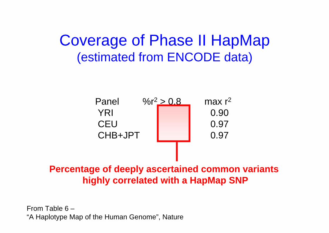
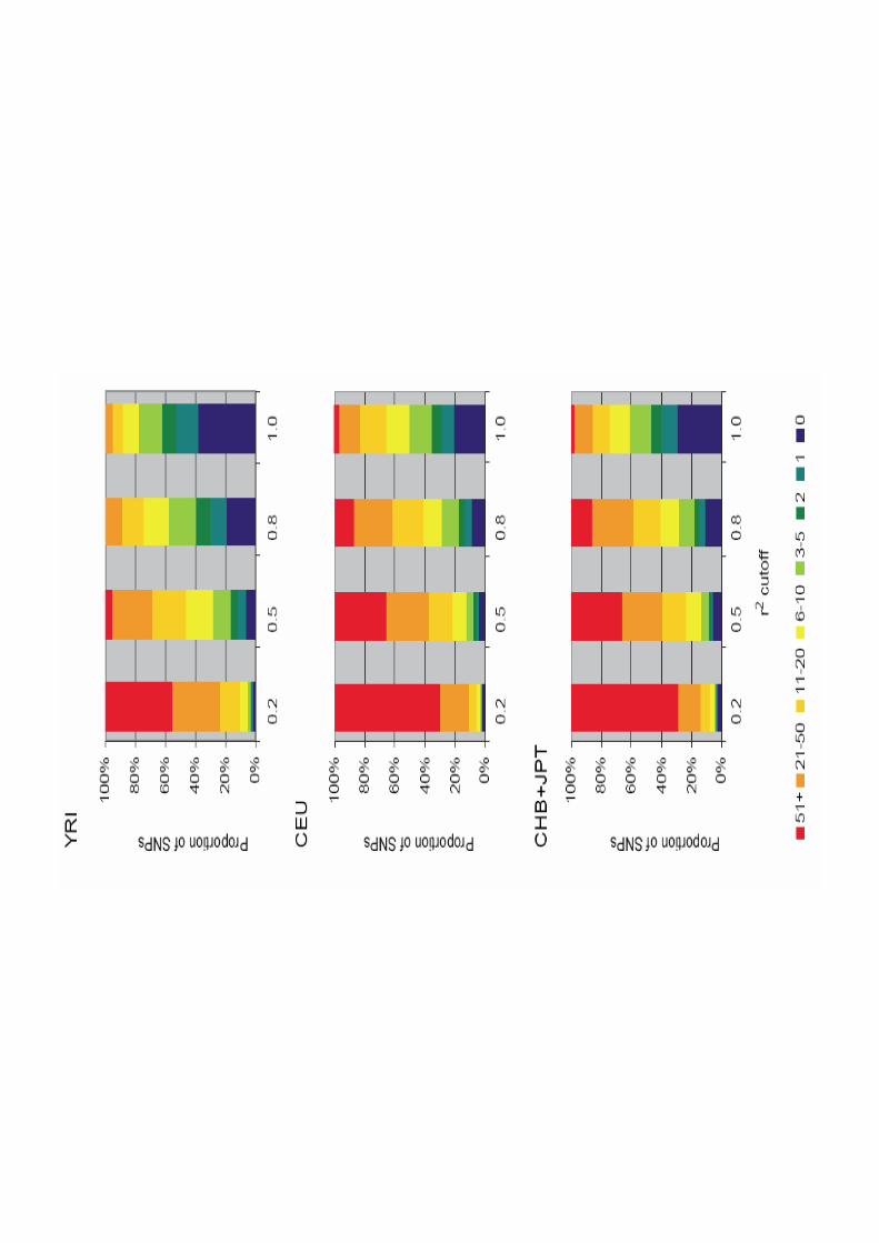
Coverage of Phase II HapMap(estimated from ENCODE data)
From Table 6 –“A Haplotype Map of the Human Genome”, Nature
Panel %r2 > 0.8 max r2
YRI 81 0.90CEU 94 0.97CHB+JPT 94 0.97
Coverage of Phase II HapMap(estimated from ENCODE data)
From Table 6 –“A Haplotype Map of the Human Genome”, Nature
Panel %r2 > 0.8 max r2
YRI 81 0.90CEU 94 0.97CHB+JPT 94 0.97
Percentage of deeply ascertained common variants highly correlated with a HapMap SNP

Coverage of Phase II HapMap(estimated from ENCODE data)
From Table 6 –“A Haplotype Map of the Human Genome”, Nature
Panel %r2 > 0.8 max r2
YRI 81 0.90CEU 94 0.97CHB+JPT 94 0.97
Average maximum correlation between a deeplyascertained variant and a neighboring HapMap SNP
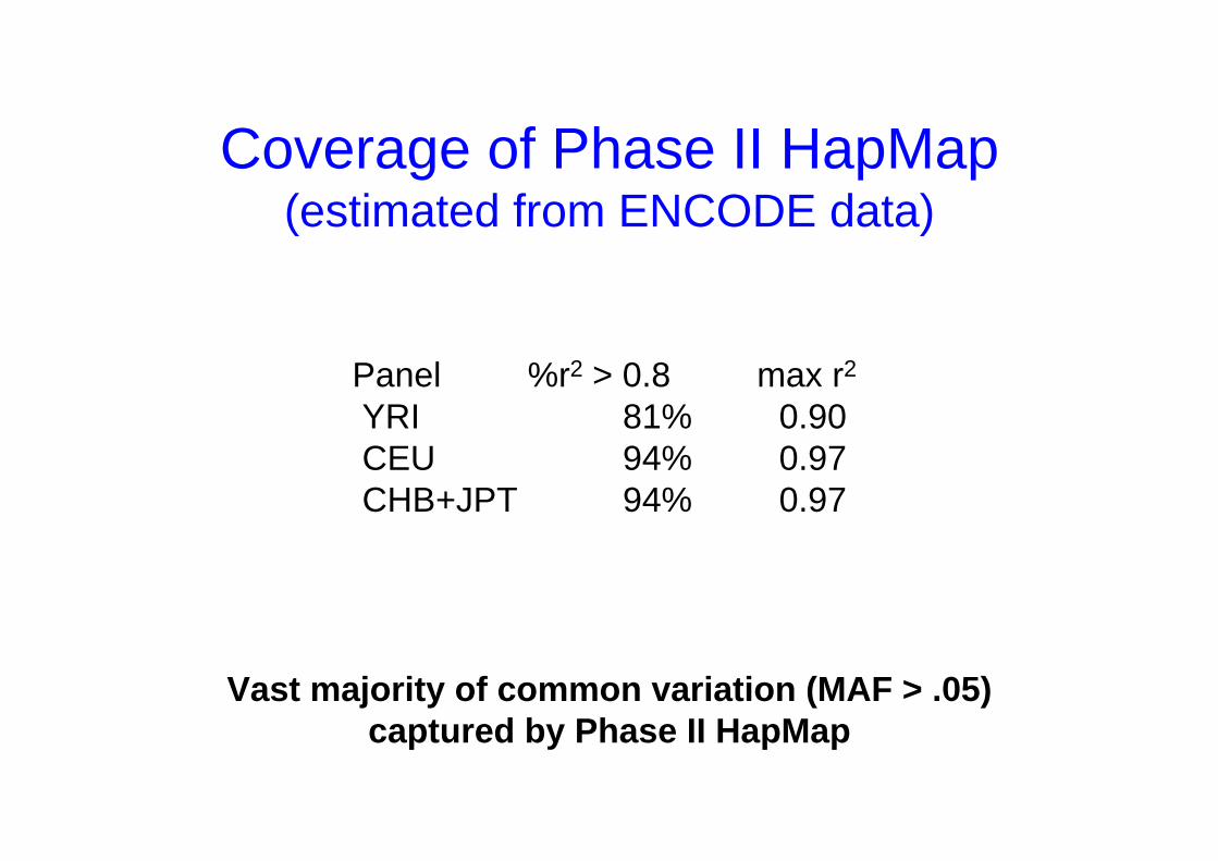
Coverage of Phase II HapMap(estimated from ENCODE data)
Vast majority of common variation (MAF > .05) captured by Phase II HapMap
Panel %r2 > 0.8 max r2
YRI 81% 0.90CEU 94% 0.97CHB+JPT 94% 0.97

HapMap Project
Draft Rel. 1 (May 2008)
Nature (2007) 449:p851
Nature (2005) 437:p1299
Reference
1.6 M (Affy 6.0 & Illumina 1M)
3.8 M
(phase I+II)
1.1 MUnique QC+ SNPs
Broad & SangerPerlegen
HapMap International Consortium
Genotyping centers
1,115 samples (11 panels)
270 samples(4 panels)
269 samples(4 panels)
Samples & POP panels
Phase 3Phase 2Phase 1
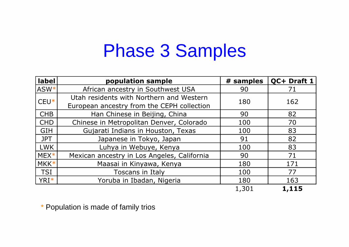
Phase 3 Samples
label population sample # samples QC+ Draft 1
ASW* African ancestry in Southwest USA 90 71
CEU*Utah residents with Northern and Western
European ancestry from the CEPH collection180 162
CHB Han Chinese in Beijing, China 90 82
CHD Chinese in Metropolitan Denver, Colorado 100 70
GIH Gujarati Indians in Houston, Texas 100 83
JPT Japanese in Tokyo, Japan 91 82
LWK Luhya in Webuye, Kenya 100 83
MEX* Mexican ancestry in Los Angeles, California 90 71
MKK* Maasai in Kinyawa, Kenya 180 171
TSI Toscans in Italy 100 77
YRI* Yoruba in Ibadan, Nigeria 180 163
1,301 1,115
* Population is made of family trios
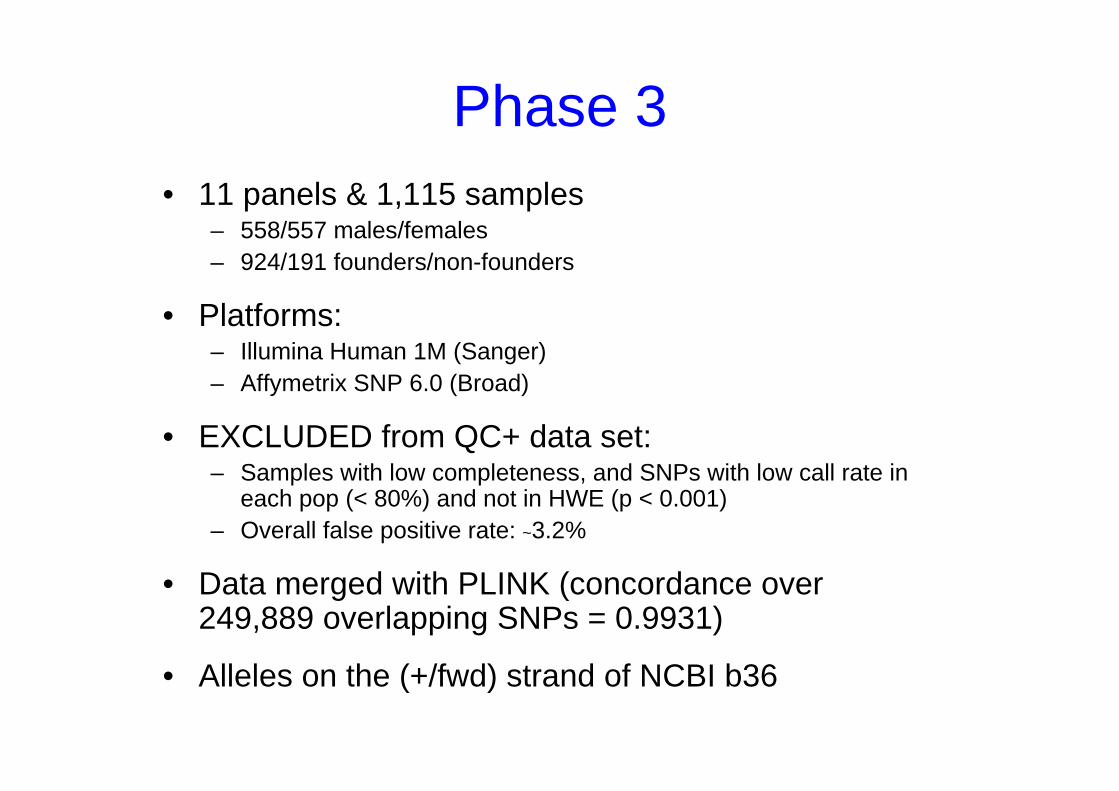
Phase 3• 11 panels & 1,115 samples
– 558/557 males/females– 924/191 founders/non-founders
• Platforms:– Illumina Human 1M (Sanger)– Affymetrix SNP 6.0 (Broad)
• EXCLUDED from QC+ data set:– Samples with low completeness, and SNPs with low call rate in
each pop (< 80%) and not in HWE (p < 0.001)– Overall false positive rate: ~3.2%
• Data merged with PLINK (concordance over 249,889 overlapping SNPs = 0.9931)
• Alleles on the (+/fwd) strand of NCBI b36

Goals of This Tutorial
• Find HapMap SNPs near a gene or region of interest (ROI)
– View patterns of LD in the ROI– Select tag SNPs in the ROI– Download information on the SNPs in ROI for use in
Haploview– Add custom tracks of association data– Create publication-quality images
• Generate customized extracts of the entire data set
• Download the entire data set in bulk
This tutorial will show you how to:

Finding HapMap SNPs in a Region of Interest
• Find the TCF7L2 gene• Identify the characterized SNPs in the region• View the patterns of LD (NCBI b35)• Pick tag SNPs (NCBI b35)• Download the region in Haploview format• Upload your own annotations & superimpose on the
HapMap• Make a customized image for publication• View GWA hits & OMIM annotations in the region
(NCBI b36)

HapMap Glossary• LD (linkage disequilibrium): For a pair of SNP alleles,
it’s a measure of deviation from random association (which assumes no recombination). Measured by D’, r2, LOD
• Phased haplotypes: Estimated distribution of SNP alleles. Alleles transmitted from Mom are in same chromosome haplotype, while Dad’s form the paternal haplotype.
• Tag SNPs: Minimum SNP set to identify a haplotype. r2= 1 indicates SNPs are redundant, so either one “tags” the other.
• Questions? [email protected]

1: Surf to the HapMap Browser1a. Go to
www.hapmap.org
1b. Select “HapMap Genome
Browser B35”
ncbi B35: full dataset (includes LD patterns)
ncbi B36: latest, new tracks (e.g., GWA hits)

2: Search for TCF7L2
2. Type search term – “TCF7L2”
Search for a gene name, a chromosome band, or a phrase like
“insulin receptor”
Region view puts your ROI in
genomic context
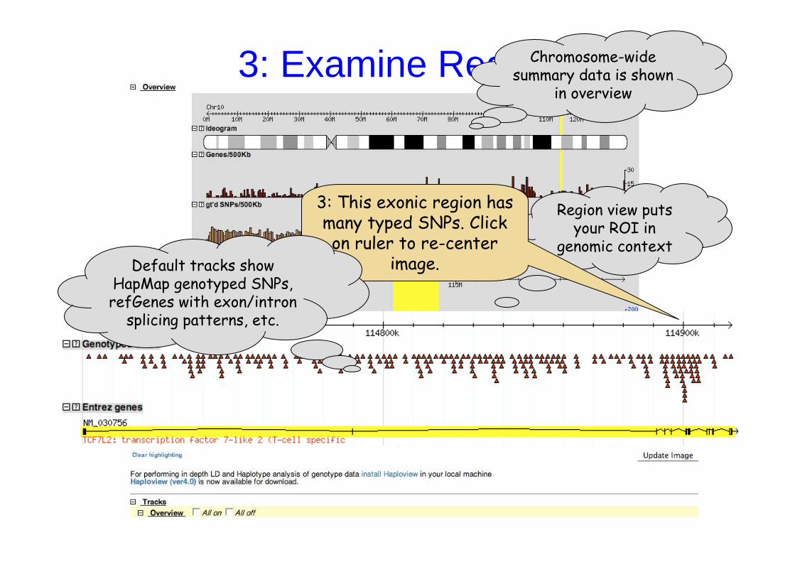
3: This exonic region has many typed SNPs. Click on ruler to re-center
image.Default tracks show HapMap genotyped SNPs, refGenes with exon/intron
splicing patterns, etc.
3: Examine RegionChromosome-wide summary data is shown
in overview

3: Examine Region (cont)
As you zoom in further, the display changes to include
more detail
Use the Scroll/Zoom
buttons and menu to change position &
magnification

As you zoom in further, the display changes to include
more detail
Use the Scroll/Zoom
buttons and menu to change position &
magnification 3: Mouse over a SNP to see allele frequency table
Click to go to SNP details page
3: Examine Region (cont) Phase III

4: Turn on LD & Haplotype Tracks
4b: Press “Update Image”
4a: Scroll down to the “Tracks” section. Turn on the LD Plot and Haplotype
Display tracks.
These sections allow you to adjust the
display and to superimpose your own data on the HapMap

5: View variation patternsTriangle plot shows LD
values using r2 or D’/LOD scores in one or more HapMap population
Phased haplotype track shows all 120 chromosomes with
alleles colored yellow and blue

7: Adjust Track Settings (on the spot)
7b. Adjust population and display settings &
press “Configure”
7a. Click on question mark preceding
track name

7: Adjust Track Settings (cont)
Select the analysis track to adjust and press “Configure”

8: Turn on Tag SNP Track
8: Activate the “tag SNP Picker” and press
“Update Image”

9: Adjust tag SNP picker
Tag SNPs are selected on the fly as you navigate
around the genome
9a: Click on question mark behind “tag SNP Picker”
Alternatively, you may select “Annotate tag SNP Picker” and press
“Configure…”

9: Adjust tag SNP picker (cont)
Select population
Select tagging algorithm and parameters
[optional] upload list of SNPs to be
included, excluded, or design scores9b: Press “Configure” to
save changes

10: Generate Reports
10: Select the desired “Download” option and
press “Go” or “Configure”
Available Downloads:• Individual Genotypes• Population Allele & Genotype
frequencies• Pairwise LD values•Tag SNPs

10: Generate Reports (cont)
The Genotype download format can be saved to disk or loaded directly
into Haploview

10: Generate Reports (cont)
The tag SNP download is the same as you get
from TAGGER
…

11: Create your own tracks
11: Upload example file: TCF7L2_annotations.txt
Example:
• Interested in T2DM genetics
• Create file with custom annotations from http://www.broad.mit.edu/diabetes and superimpose on the HapMap
Detailed help on the format is under the
“Help” link
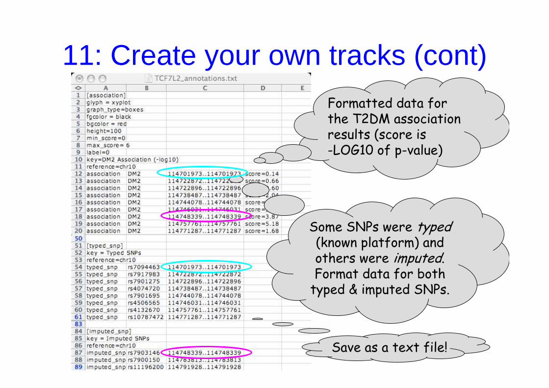
11: Create your own tracks (cont)
Save as a text file!
Some SNPs were typed(known platform) and others were imputed. Format data for both typed & imputed SNPs.
Formatted data for the T2DM association results (score is-LOG10 of p-value)

11: Create your own tracks (cont)

Make edits on your own browser window by clicking
on “Edit File…”
11: Create your own tracks (cont)

11: Create your own tracks (cont)

12: Create Image for Publication
12a. Click on “High-res Image”
Click on the +/- sign to
hide/show a section
Mouse over a track until a cross appears.
Click on track name to drag track up or down.
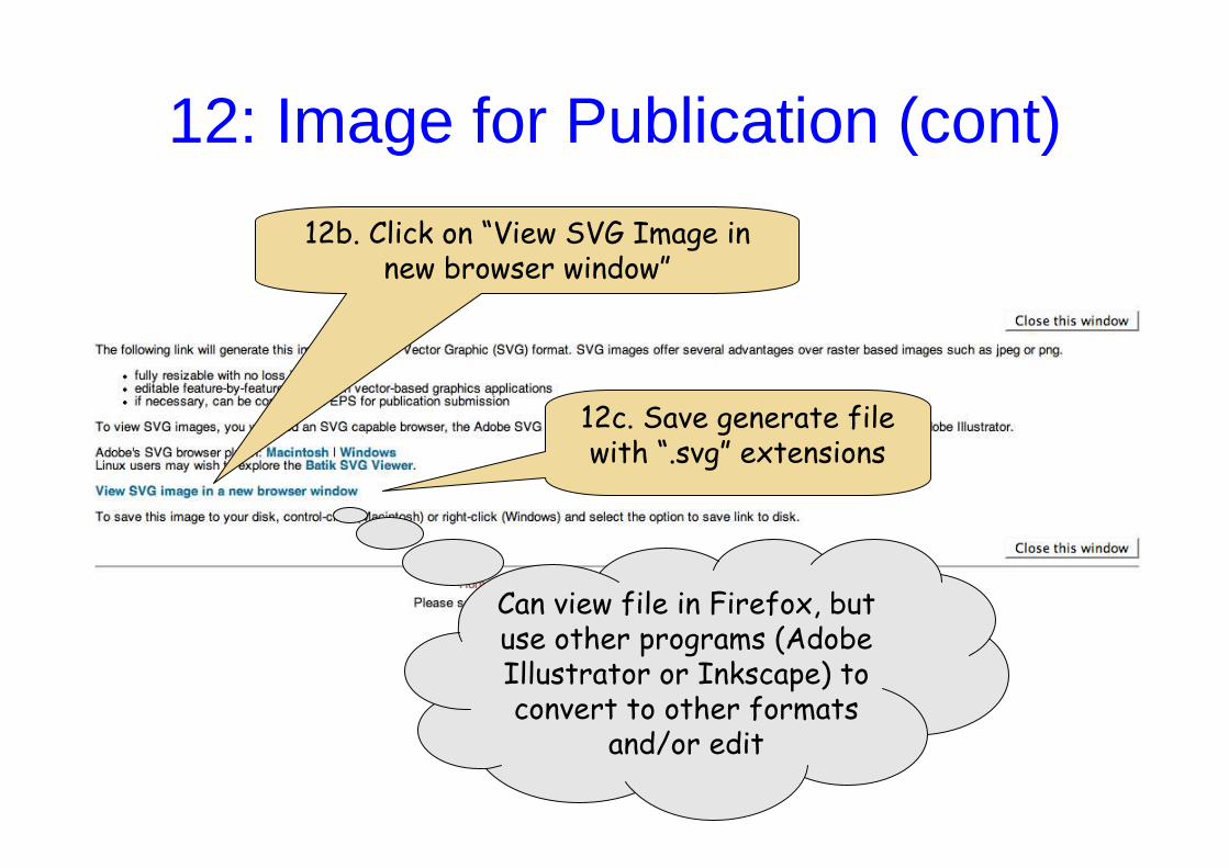
Can view file in Firefox, but use other programs (Adobe Illustrator or Inkscape) to convert to other formats
and/or edit
12b. Click on “View SVG Image in new browser window”
12c. Save generate file with “.svg” extensions
12: Image for Publication (cont)
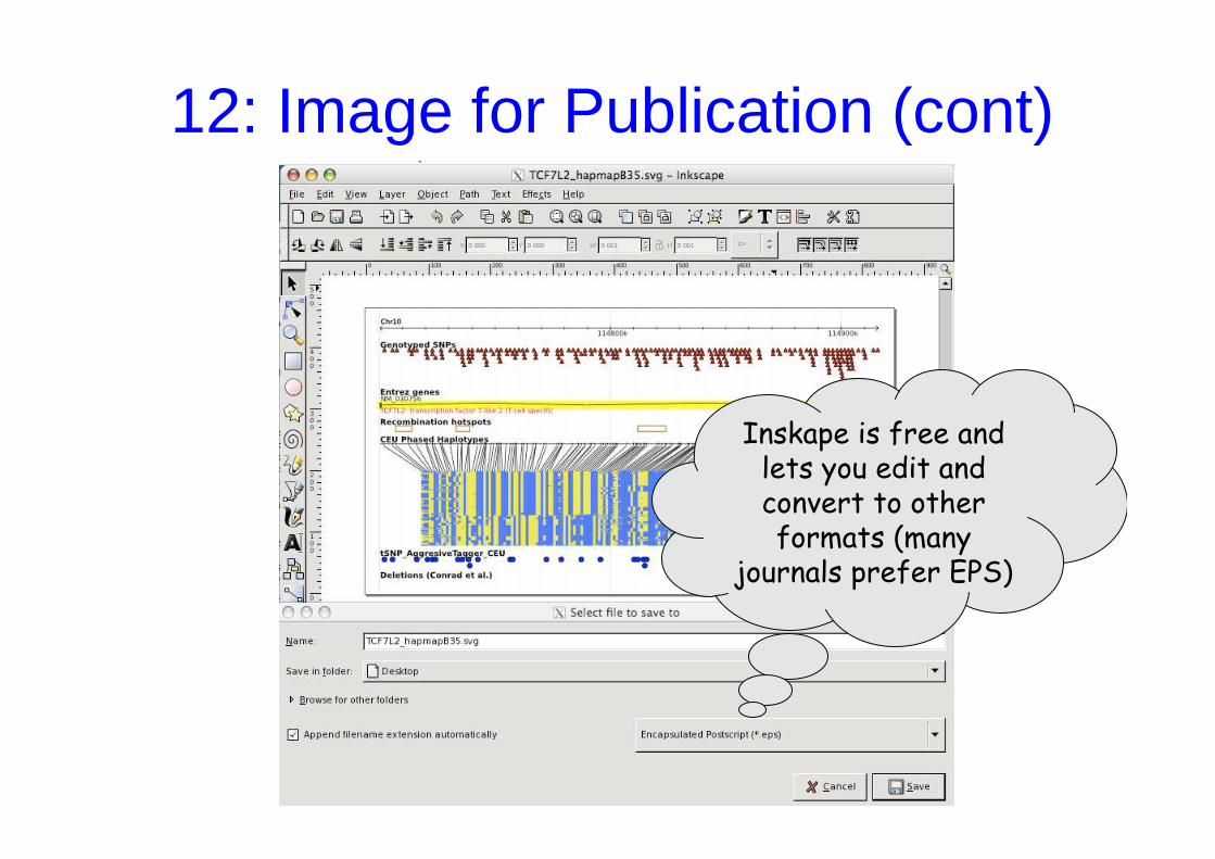
Inskape is free and lets you edit and convert to other formats (many
journals prefer EPS)
12: Image for Publication (cont)
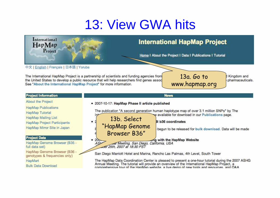
13: View GWA hits
13a. Go to www.hapmap.org
13b. Select “HapMap Genome
Browser B36”

13: View GWA hits (cont)
13c. Type search term - “FTO”
Default tracks for B36 include GWA hits, OMIM
predicted associations, and Reactome pathways

14: Read PubMed abstracts for GWA hits
14a: Mouse over a GWA hit to learn more about the
association
14b: Click on the GWA hit to see the study’s PubMed
abstract
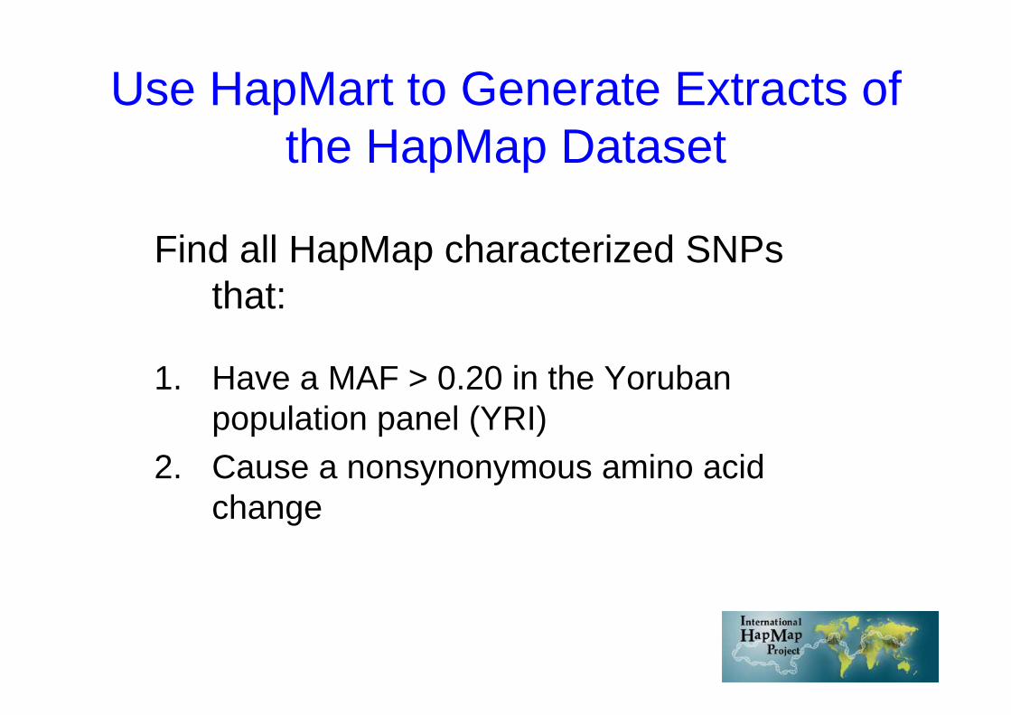
Use HapMart to Generate Extracts of the HapMap Dataset
Find all HapMap characterized SNPs that:
1. Have a MAF > 0.20 in the Yoruban population panel (YRI)
2. Cause a nonsynonymous amino acid change

1. Go to hapmart.hapmap.org
1. From www.hapmap.orgclick on “HapMart”

2. Select data source and population of interest
2a. Choose Yoruba population or “All Populations”
2b. Press “Next”
Use schema menu to select dataset

3. Select the desired filters
3a. Check “Allele Frequency Filter” and
select MAF >= 0.2
3b. Select “SNPs found in Exons – non synonymous
coding SNPs”
3c. Press “Next”
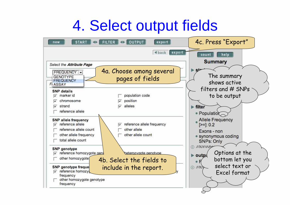
4. Select output fields
4b. Select the fields to include in the report.
4c. Press “Export”
The summary shows active
filters and # SNPs to be output
Options at the bottom let you select text or Excel format
4a. Choose among several pages of fields

5. Download report

Bulk downloads: Download the Complete Data
• Download the entire HapMap data set to your own computer

1. Surf to www.hapmap.org
1. From www.hapmap.org, click on “Bulk Data
Download”
Or directly click on “Data”
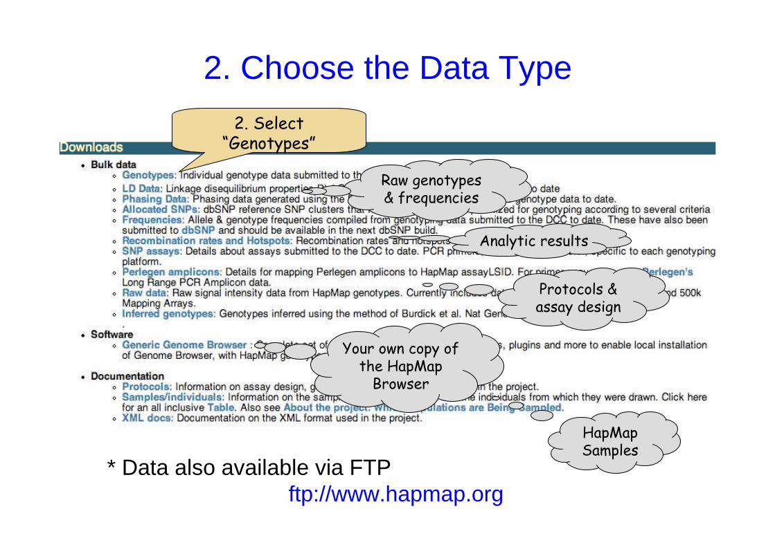
2. Choose the Data Type
Raw genotypes & frequencies
Analytic results
HapMap Samples
Protocols & assay design
Your own copy of the HapMap
Browser
2. Select “Genotypes”
* Data also available via FTPftp://www.hapmap.org

3. Choose the dataset of interest
Available Genotype Datasets:• Non-redundant: QC+ filtered & redundant data removed• Filtered-redundant: QC+ filtered; duplicated data not removed• Unfiltered-redundant: Includes assays that failed QC
3. Select latest build, fwd_strand orientation,
and “non-redundant”
fwd_strand => same as NCBI reference assemblyrs_strand => same as in dbSNP

Applying the HapMap
• Study design - tagging• Study coverage evaluation• Study analysis - improving association
testing• Study interpretation
– Comparison of multiple studies– Connection to genes/genomic features– Integration with expression and other functional
data
• Other uses of HapMap data– Admixture, LOH, selection

Tagging from HapMap
• Since HapMap describes the majority of common variation in the genome, choosing non-redundant sets of SNPs from HapMap offers considerable efficiency without power loss in association studies

Pairwise tagging
Tags:
SNP 1SNP 3SNP 6
3 in total
Test for association:
SNP 1SNP 3SNP 6
A/T1
G/A2
G/C3
T/C4
G/C5
A/C6
high r2 high r2 high r2
AATT
GC
CG
GC
CG
TCCC
ACCC
GC
CG
TCCC
GGAA
GGAA
After Carlson et al. (2004) AJHG 74:106
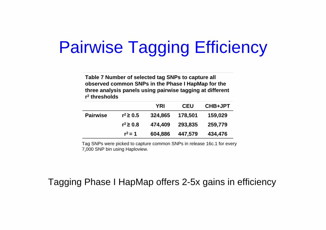
Pairwise Tagging Efficiency
Table 7 Number of selected tag SNPs to capture all observed common SNPs in the Phase I HapMap for the three analysis panels using pairwise tagging at different r2 thresholds
YRI CEU CHB+JPT
Pairwise r2 ≥ 0.5 324,865 178,501 159,029
r2 ≥ 0.8 474,409 293,835 259,779
r2 = 1 604,886 447,579 434,476
Tag SNPs were picked to capture common SNPs in release 16c.1 for every 7,000 SNP bin using Haploview.
Tagging Phase I HapMap offers 2-5x gains in efficiency

Tags:
SNP 1SNP 3SNP 6
3 in total
Test for association:
SNP 1SNP 3SNP 6
Use of haplotypes can improve genotyping efficiency
Tags:
SNP 1SNP 3
2 in total
Test for association:
SNP 1 captures 1+2SNP 3 captures 3+5
“AG” haplotype captures SNP 4+6
AATT
GC
CG
GC
CG
TCCC
ACCC
GC
CG
TCCC
GGAA
GGAA
ACCC
A/T1
G/A2
G/C3
T/C4
G/C5
A/C6
tags in multi-marker test should be conditional on significance
of LD in order to avoid overfitting

Efficiency and powerR
elat
ive
pow
er (
%)
Average marker density (per kb)
tag SNPs
randomSNPs
P.I.W. de Bakker et al. (2005) Nat Genet Advance Online Publication 23 Oct 2005
~300,000 tag SNPsneeded to cover commonvariation in whole genome
in CEU

How to pick tag SNPs?
• What is the genetic hypothesis? Which variants do you want to test for a role in disease?– functional annotation (coding SNPs)– allele frequency (HapMap ascertainment)– previously implicated associations
• Go to http://www.hapmap.org – DCC supported interactive tagging
• Export HapMap data into tools such as Tagger, Haploview (www.broad.mit.edu/mpg)

Will tag SNPs picked from HapMap apply to other population samples?
Population differences add very little inefficiencyPlatform presentation: Paul de Bakker (#223: Sat 9.30)
CEUCEU
Whites fromLos Angeles, CA
Whites fromLos Angeles, CA Botnia, FinlandBotnia, Finland
CEUCEUCEUCEU
Utah residents with European ancestry
(CEPH)
Utah residents with European ancestry
(CEPH)

Applying the HapMap
• Study design - tagging• Study coverage evaluation• Study analysis - improving association
testing• Study interpretation
– Comparison of multiple studies– Connection to genes/genomic features– Integration with expression and other functional
data
• Other uses of HapMap data– Admixture, LOH, selection

Genome-wide association coverage
• If genome-wide products are typed on the HapMap sample panel, the SNPs on HapMap not included in the panel provide an evaluation for the coverage of the product– ENCODE (deep ascertainment) – Phase II (dense, genome-wide)

Further Information
• HapMap Publications & Guidelineshttp://hapmap.cshl.org/publications.html.en
• Past tutorials & user’s guide to HapMap.orghttp://www.hapmap.org/tutorials.html.en