HAL Id: inria-00000661https://hal.inria.fr/inria-00000661v1

Submitted on 10 Nov 2005 (v1), last revised 9 Jan 2008 (v2)

HAL is a multi-disciplinary open accessarchive for the deposit and dissemination of sci-entific research documents, whether they are pub-lished or not. The documents may come fromteaching and research institutions in France orabroad, or from public or private research centers.

L’archive ouverte pluridisciplinaire HAL, estdestinée au dépôt et à la diffusion de documentsscientifiques de niveau recherche, publiés ou non,émanant des établissements d’enseignement et derecherche français ou étrangers, des laboratoirespublics ou privés.

Resource analysis by sup-interpretationJean-Yves Marion, Romain Péchoux

To cite this version:Jean-Yves Marion, Romain Péchoux. Resource analysis by sup-interpretation. Masami Hagiya, PhilipWadler. Eighth International Symposium on Functional and Logic Programming - FLOPS 2006, Apr2006, Fuji Susono/Japan, Japan. Springer, 3945 (3945), pp.163–176, 2006, Lecture Notes in ComputerScience. <inria-00000661v1>

Resource analysis by sup-interpretation

Jean-Yves Marion and Romain Pechoux

Loria, Calligramme project, B.P. 239, 54506 Vandœuvre-les-Nancy Cedex, France,

and Ecole Nationale Superieure des Mines de Nancy, INPL, France.

Jean-Yves.Marion@loria.fr Romain.Pechoux@loria.fr5

Abstract. We propose a new method to control memory resources by

static analysis. For this, we introduce the notion of sup-interpretation

which bounds from above the size of function outputs. This method

applies to first order functional programming with pattern matching.

This work is related to quasi-interpretations but we are now able to10

determine resources of more algorithms and it is easier to perform an

analysis with this new tools.

1 Introduction

This paper deals with general investigation on program complexity analysis. It

introduces the notion of sup-interpretation, a new tool that provides an upper15

bound on the size of every stack frame if the program is non-terminating, and

establishes an upper bound on the size of function outputs if the program is

terminating.

A sup-interpretation of a program is a partial assignment of function symbols,

which ranges over reals and which bounds the size of the computed values.20

The practical issue is to provide program static analysis in order to guarantee

space resources that a program consumes during an execution. There is no need

to say that this is crucial for at least many critical applications, and have strong

impact in computer security. There are several approaches related in [18], which

are trying to solve the same problem. The first protection mechanism is by25

monitoring computations. However, if the monitor is compiled with the program,

it could crash unpredictably by memory leak. The second is the testing-based

approach, which is complementary to static analysis. Indeed, testing provides a

2

lower bound on the memory while static analysis gives an upper bound. The gap

between both bounds is of some value in practical. Lastly, the third approach30

is type checking done by a bytecode verifier. In an untrusded environment (like

embedded systems), the type protection policy (Java or .Net) does not allow

dynamic allocation. Our approach is an attempt to control resources, and provide

a proof certificate, of a high-level language in such a way that the compiled code

is safe wrt memory overflow. Thus, we capture and deal with memory allocation35

features. Similar approaches are the one of Hofmann [12, 13] and the one of

Aspinall and Compagnoni [5].

For that purpose we consider first order functional programming language

with pattern matching but we hardly believe that such a method could be applied

to other languages such as resource bytecode verifier by following the lines of [2],40

language with synchronous cooperative threads as in [3] or first order functional

language including streams as in [11] .

The notion of sup-interpretation can be seen as a kind of annotation provided

in the code by the programmer. Sup-interpretations strongly inherit from the no-

tion of quasi-interpretation developed by Bonfante, Marion and Moyen in [8, 9,45

17]. Consequently the notion of sup-interpretation is heiress of the notion of

polynomial interpretation used to prove termination of programs in [10, 14] and

more recently in [6, 16]. Quasi-interpretation, like sup-interpretation, provides

a bound over function outputs by static analysis for first order functional pro-

grams. Quasi-interpretation was developed with the aim to pay more attention50

to the algorithmic aspects of complexity than to the functional (or extensional)

one and then it is part of study of the implicit complexity of programs.

However both notions differ for two reasons. First, the sup-interpretations are

partial assignments which does not satisfy the subterm property, and this allows

to capture a larger class of algorithms. In fact, programs computing logarithm55

or division admits a sup-interpretation but have no quasi-interpretation. Second,

the sup-interpretation is a partial assignment over the set of function symbols

of a program, whereas the quasi-interpretation is a total assignment on function

symbols. On the other hand, sup-interpretations come with a companion, which

is a weight to measure argument size of recursive calls involved in a program60

run. Such constraints are developped thanks to the notion of dependency pairs

3

by Arts and Giesl [4]. The dependency pairs were initially introduced for prov-

ing termination of term rewriting systems automatically. Even if this paper no

longer focuses on termination, the notion of dependency pair is used for forcing

the program to compute in polynomial space. There is a very strong relation65

between termination and complexity. Indeed,both for proving some complexity

bounds and for proving termination, we need to control the arguments occurring

in a function recursive call. Since we try to control the arguments of a recursive

call together, the sup-interpretation is closer from the dependency pairs method

than from the size-change principle method of [15] which consider the arguments70

of a recursive call separately. Section 2 introduces the first order functional lan-

guage and its semantics. Section 3 defines the main notions of sup-interpretation

and weight using to bound the size of a program outputs. Section 4 presents the

notion of dependency pairs by Arts and Giesl [4] and the ensuing notion of fra-

ternity used to control the size of values added by recursive calls. In section 5, we75

define the notion of polynomial and additive assignments for sup-interpretations

and weights. Finally, section 6 introduces the notion of friendly programs and

the main theorems of this paper providing a polynomial bound on the values

computed by friendly programs. The full paper with all proofs is available at

http://www.loria.fr/∼pechoux.80

2 First order functional programming

2.1 Syntax of programs

We define a generic first order functional programming language. The vocabulary

Σ = 〈Cns,Op,Fct〉 is composed of three disjoint domains of symbols. The arity

of a symbol is the number n of arguments that it takes. The set of programs are

defined by the following grammar.

Programs 3p ::= def 1, · · · , def m

Definitions 3 def ::= f(x1, · · · , xn) = ef

Expression 3 e ::= x | c(e1, · · · , en) | op(e1, · · · , en) | f(e1, · · · , en)

| Case e1, · · · , en of p1 → e1 . . . p` → e`

Patterns 3 p ::= x | c(p1, · · · , pn)

4

where c ∈ Cns is a constructor, op ∈ Op is an operator, f ∈ Fct is a

function symbol, and pi is a sequence of n patterns. Throughout, we generalize

this notation to expressions and we write e to express a sequence of expressions,85

that is e = e1, . . . , en, for some n clearly determined by the context.

The set of variables Var is disjoint from Σ and x ∈ Var. In a definition, ef

is called the body of f. A variable of ef is either a variable in the parameter

list x1, · · · , xn of the definition of f or a variable which occurs in a pattern

of a case definition. In a case expression, patterns are not overlapping. The90

program’s main function symbol is the first function symbol in the program’s

list of definitions. We usually don’t make the distinction between this main

symbol and the program symbol p.

Lastly, it is convenient, because it avoids tedious details, to restrict case

definitions in such way that an expression involved in a Case expression does95

not contain nested Case (In other word, an expression ej does not contain an

expression Case ). This is not a severe restriction since a program involving

nested Case can be transformed in linear time in its size into an equivalent

program without the nested case construction.

2.2 Semantics100

The set Values is the constructor algebra freely generated from Cns.

Values 3 v ::= c | c(v1, · · · , vn) c ∈ Cns

Put Values∗ = Values ∪ {Err} where Err is the value associated when an

error occurs. Each operator op of arity n is interpreted by a function JopK

from Valuesn to Values∗. Operators are essentially basic partial functions like

destructors or characteristic functions of predicates like =. The destructor tl

illustrates the purpose of Err when it satisfies Jtl(nil)K = Err.105

The computational domain is Values# = Values ∪ {Err,⊥} where ⊥ means

that a program is non-terminating. The language has a closure-based call-by-

value semantics which is displayed in Figure 1. A few comments are necessary.

A substitution σ is a finite function from variables to Values. The application

of a substitution σ to an expression e is noted eσ.110

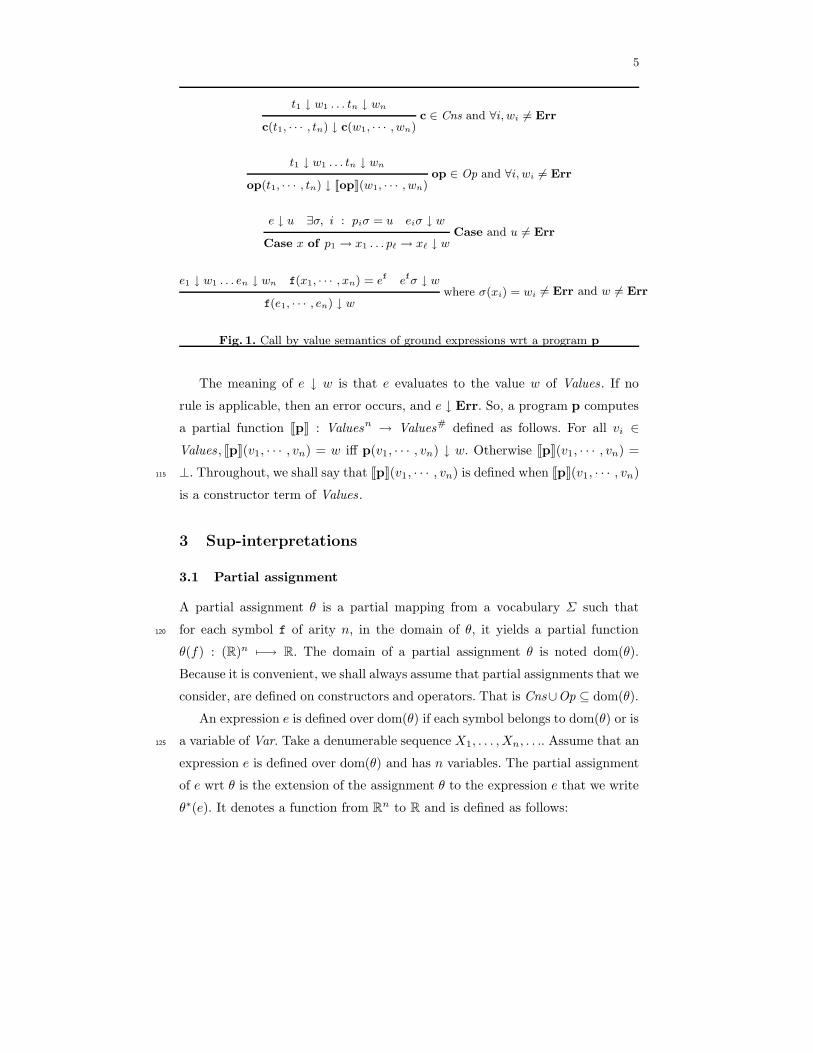
5

t1 ↓ w1 . . . tn ↓ wn

c ∈ Cns and ∀i, wi 6= Errc(t1, · · · , tn) ↓ c(w1, · · · , wn)

t1 ↓ w1 . . . tn ↓ wn

op ∈ Op and ∀i, wi 6= Errop(t1, · · · , tn) ↓ JopK(w1, · · · , wn)

e ↓ u ∃σ, i : piσ = u eiσ ↓ wCase and u 6= Err

Case x of p1 → x1 . . . p` → x` ↓ w

e1 ↓ w1 . . . en ↓ wn f(x1, · · · , xn) = ef

efσ ↓ w

where σ(xi) = wi

f(e1, · · · , en) ↓ w6= Err and w 6= Err

Fig. 1. Call by value semantics of ground expressions wrt a program p

The meaning of e ↓ w is that e evaluates to the value w of Values. If no

rule is applicable, then an error occurs, and e ↓ Err. So, a program p computes

a partial function JpK : Valuesn → Values# defined as follows. For all vi ∈

Values , JpK(v1, · · · , vn) = w iff p(v1, · · · , vn) ↓ w. Otherwise JpK(v1, · · · , vn) =

⊥. Throughout, we shall say that JpK(v1, · · · , vn) is defined when JpK(v1, · · · , vn)115

is a constructor term of Values.

3 Sup-interpretations

3.1 Partial assignment

A partial assignment θ is a partial mapping from a vocabulary Σ such that

for each symbol f of arity n, in the domain of θ, it yields a partial function120

θ(f) : (R)n 7−→ R. The domain of a partial assignment θ is noted dom(θ).

Because it is convenient, we shall always assume that partial assignments that we

consider, are defined on constructors and operators. That is Cns∪Op ⊆ dom(θ).

An expression e is defined over dom(θ) if each symbol belongs to dom(θ) or is

a variable of Var. Take a denumerable sequence X1, . . . , Xn, . . .. Assume that an125

expression e is defined over dom(θ) and has n variables. The partial assignment

of e wrt θ is the extension of the assignment θ to the expression e that we write

θ∗(e). It denotes a function from Rn to R and is defined as follows:

6

1. If xi is a variable of Var, let θ∗(xi) = Xi

2. If b is a 0-ary symbol of Σ, then θ∗(b) = θ(b).130

3. If e is a sequence of n expressions, then θ∗(e) = max(θ∗(e1), . . . , θ∗(en))

4. If e is a Case expression of the shape Case e of p1 → e1 . . . p` → e`,

θ∗(e) = max(θ∗(e), θ∗(e1), . . . , θ∗(e`))

5. If f is a symbol of arity n > 0 and e1, · · · , en are expressions, then

θ∗(f(e1, · · · , en)) = θ(f)(θ∗(e1), . . . , θ∗(en))

3.2 Sup-interpretation

Definition 1 (Sup-interpretation). A sup-interpretation is a partial assign-

ment θ which verifies the three conditions below :135

1. The assignment θ is weakly monotonic. That is, for each symbol f ∈ dom(θ),

the function θ(f) satisfies

∀i = 1, . . . , n Xi ≥ Yi ⇒ θ(f)(X1, · · · , Xn) ≥ θ(f)(Y1, · · · , Yn)

2. For each v ∈ Values,

θ∗(v) ≥ |v|

The size of an expression e is noted |e| and is defined by |c| = 0 where c is

a 0-ary symbol and |b(e1, . . . , en)| = 1 +∑

i |ei| where b is a n-ary symbol.

3. For each symbol f ∈ dom(θ) of arity n and for each value v1, . . . , vn of

Values, if JfK(v1, . . . , vn) is defined, that is JfK(v1, . . . , vn) ∈ Values, then

θ∗(f(v1, . . . , vn)) ≥ θ∗(JfK(v1, . . . , vn))

Now an expression e admits a sup-interpretation θ if e is defined over dom(θ).

The sup-interpretation of e wrt θ is θ∗(e).

Intuitively, the sup-interpretation is a special program interpretation. Instead140

of yielding the program denotation, a sup-interpretation provides an approxima-

tion from above of the size of the outputs of the function denoted by the program.

7

Lemma 1. Let e be an expression with no variable and which admits a sup-

interpretation θ. Assume that JeK is defined. We then have

θ∗(JeK) ≤ θ∗(e)

Proof. The proof is done by structural induction on expression. The base case

is a consequence of Condition 2 of Definition 1.

Take an expression e = f(e1, · · · , en) that has a sup-interpretation θ. By

induction hypothesis (IH), we have θ∗(ei) ≥ θ∗(JeiK). Now,

θ∗(e) = θ(f)(θ∗(e1), ..., θ∗(en)) by definition of θ∗

≥ θ(f)(θ∗(Je1K), ..., θ∗(JenK)) by 1 of Dfn 1 and (IH)

= θ∗(f(Je1K, ..., JenK)) by definition of θ∗

≥ θ∗(JfK(Je1K, ..., JenK)) by 3 of Dfn 1

= θ∗(JeK)

Given an expression e, we define ‖e‖ thus:

‖e‖ =

|JeK| if JeK is defined

0 otherwise

Corollary 1. Let e be an expression with no variable and which admits a sup-

interpretation θ. Assume that JeK is defined. We then have

‖e‖ ≤ θ∗(e)

Proof.

θ∗(e) ≥ θ∗(JeK) by Lemma 1

≥ ‖e‖ by Condition 2 of Dfn 1

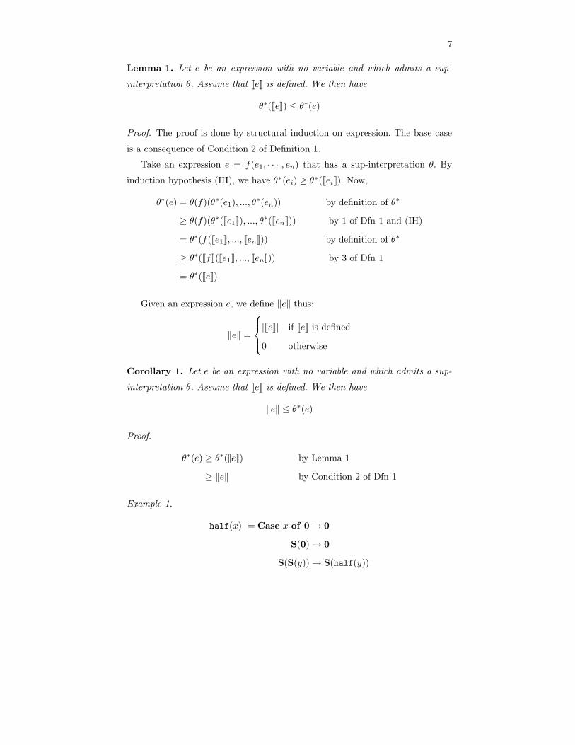
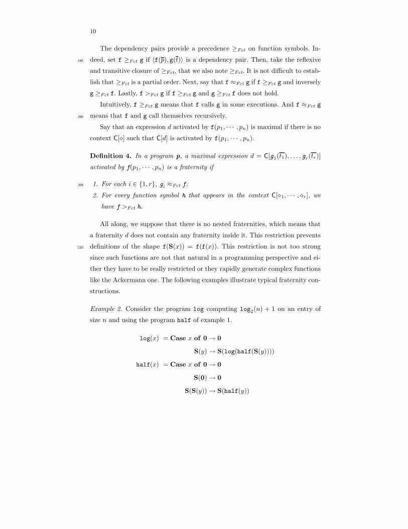
Example 1.

half(x) = Case x of 0→ 0

S(0)→ 0

S(S(y))→ S(half(y))

8

In this example, the function half computes bn/2c on an entry of size n. So by145

taking θ(S)(X) = X+1 and θ(half)(X) = X/2, we define a sup-interpretation of

the function symbol half. In fact, those functions are monotonic. For every unary

value v of size n, θ∗(v) = n ≥ n = |v| by definition of θ(S), so that condition 2

on sup-interpretation is satisfied. Finally, it remains to check that for every value

v, θ∗(half(v)) ≥ θ∗(Jhalf(v)K). For a value v of size n, we have by definition of150

θ∗ that θ∗(half(v)) = θ∗(v)/2 = n/2 and θ∗(Jhalf(v)K) = ‖half(v)‖ = bn/2c.

Since n/2 ≥ bn/2c, condition 3 of sup-interpretation is satisfied. Notice that such

a sup-interpretation is not a quasi-interpretation (a fortiori not an interpretation

for proof termination) since it has not the subterm property.

3.3 Weight155

The weight allows us to control the size of the arguments in recursive calls. A

weight is an assignment having the subterm property but no longer giving a

bound on the size of a value computed by a function. Intuitively, whereas the

sup-interpretation controls the size of the computed values, the weight can be

seen as a control point for the computation of recursive calls.160

Definition 2 (Weight). A weight ω is a partial assignment which ranges over

Fct. To a given function symbol f of arity n it assigns a total function ωf from

Rn to R which satisfies:

1. ωf is weakly monotonic.

∀i = 1, . . . , n, Xi ≥ Yi ⇒ ωf(. . . , Xi, . . .) ≥ ωf(. . . , Yi, . . .)

2. ωf has the subterm property

∀i = 1, . . . , n, ωf(. . . , Xi, . . .) ≥ Xi

The weight of a function is often taken to be the maximum or the sum

functions.165

The weight is useful to control the number of occurrences of a recursive call .

Indeed, the monotonicity property combined with the fact that a weight ranges

over function symbols ensures suitable properties on the number of occurrences

9

of a loop in a program when we consider the constraints given in section 6.

Moreover, the subterm property ensures to control the size of each argument in170

a recursive calls, in opposition to the size-change principle as mentioned in the

introduction.

4 Fraternities

In this section we define fraternies which are an important notion based on

dependency pairs, that Arts and Giesl [4] introduced to prove termination au-175

tomatically. Fraternities allows to tame the size of arguments of recursive calls.

A context is an expression C[�1, · · · , �r] containing one occurrence of each �i.

Here, we suppose that the �i’s are new symbols which are not in Σ nor in Var.

The substitution of each �i by an expression di is noted C[d1, · · · , dr].180

Assume that f(x1, · · · , xn) = ef is a definition of a program. An expression

d is activated by f(p1, · · · , pn) where the pi’s are patterns if there is a context

with one hole C[�] such that:

– If ef is a compositional expression (that is with no case definition inside it),

then ef = C[d]. In this case, p1 = x1 . . . pn = xn.185

– Otherwise, ef = Case x1, · · · , xn of q1 → e1 . . . q` → e`, then there is a

position j such that ej = C[d]. In this case, p1 = qj,1 . . . pn = qj,n where

qj = qj,1 . . . qj,n.

At first glance, this definition may look a bit tedious. However, it is practical

in order to predict the computational data flow involved. Indeed, an expression190

is activated by f(p1, · · · , pn) when f(v1, · · · , vn) is called and each vi matches

the corresponding pattern pi.

Definition 3. Assume that p is a program. A dependency pair

〈f(p1, · · · , pn), g(t1, · · · , tm)〉

is a couple such that g(t1, · · · , tm) is activated by f(p1, · · · , pn).

10

The dependency pairs provide a precedence ≥Fct on function symbols. In-

deed, set f ≥Fct g if 〈f(p), g(t)〉 is a dependency pair. Then, take the reflexive195

and transitive closure of ≥Fct, that we also note ≥Fct. It is not difficult to estab-

lish that ≥Fct is a partial order. Next, say that f ≈Fct g if f ≥Fct g and inversely

g ≥Fct f. Lastly, f >Fct g if f ≥Fct g and g ≥Fct f does not hold.

Intuitively, f ≥Fct g means that f calls g in some executions. And f ≈Fct g

means that f and g call themselves recursively.200

Say that an expression d activated by f(p1, · · · , pn) is maximal if there is no

context C[�] such that C[d] is activated by f(p1, · · · , pn).

Definition 4. In a program p, a maximal expression d = C[g1(t1), . . . , gr(tr)]

activated by f(p1, · · · , pn) is a fraternity if

1. For each i ∈ {1, r}, gi ≈Fct f.205

2. For every function symbol h that appears in the context C[�1, · · · , �r], we

have f >Fct h.

All along, we suppose that there is no nested fraternities, which means that

a fraternity d does not contain any fraternity inside it. This restriction prevents

definitions of the shape f(S(x)) = f(f(x)). This restriction is not too strong210

since such functions are not that natural in a programming perspective and ei-

ther they have to be really restricted or they rapidly generate complex functions

like the Ackermann one. The following examples illustrate typical fraternity con-

structions.

Example 2. Consider the program log computing log2(n) + 1 on an entry of

size n and using the program half of example 1.

log(x) = Case x of 0→ 0

S(y)→ S(log(half(S(y))))

half(x) = Case x of 0→ 0

S(0)→ 0

S(S(y))→ S(half(y))

11

This program admits two fraternities S(log[half(S(y))]) and S[half(y)] since215

log >Fct half.

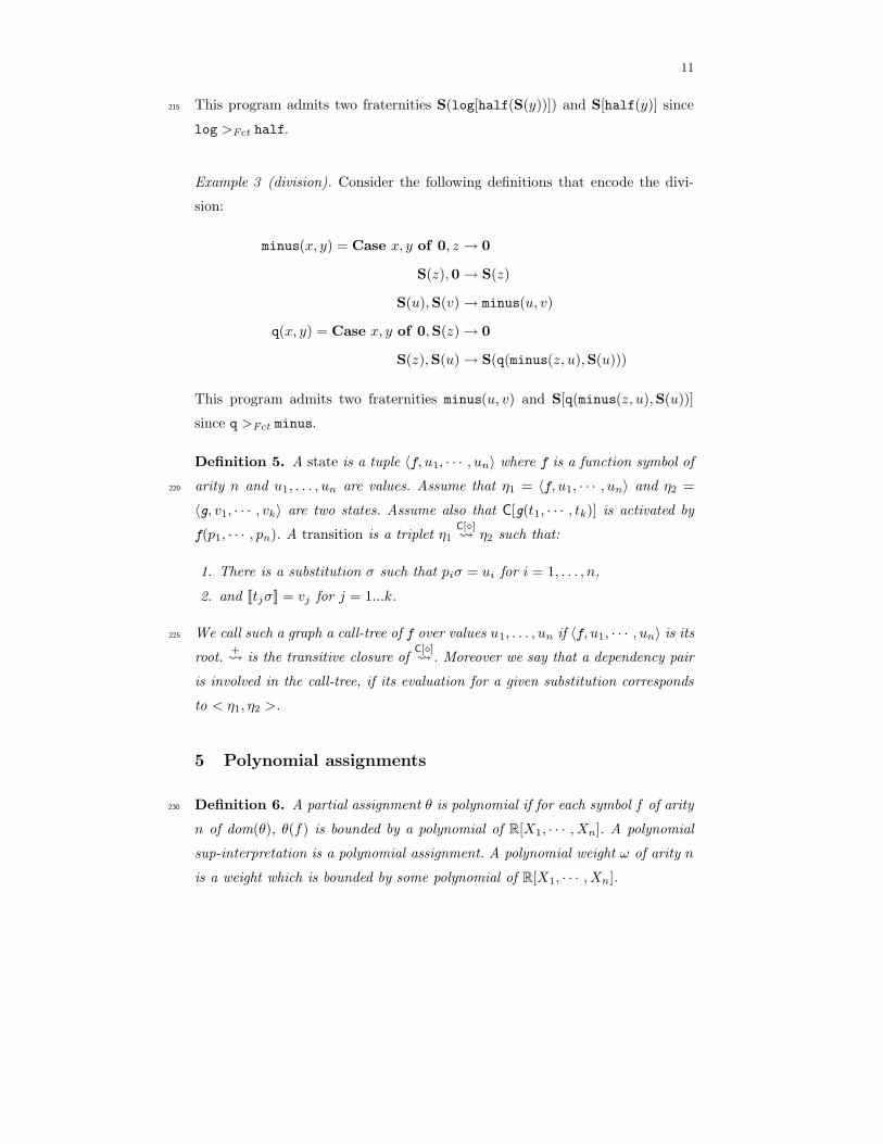
Example 3 (division). Consider the following definitions that encode the divi-

sion:

minus(x, y) = Case x, y of 0, z → 0

S(z),0→ S(z)

S(u),S(v)→ minus(u, v)

q(x, y) = Case x, y of 0,S(z)→ 0

S(z),S(u)→ S(q(minus(z, u),S(u)))

This program admits two fraternities minus(u, v) and S[q(minus(z, u),S(u))]

since q >Fct minus.

Definition 5. A state is a tuple 〈f, u1, · · · , un〉 where f is a function symbol of

arity n and u1, . . . , un are values. Assume that η1 = 〈f, u1, · · · , un〉 and η2 =220

〈g, v1, · · · , vk〉 are two states. Assume also that C[g(t1, · · · , tk)] is activated by

f(p1, · · · , pn). A transition is a triplet η1C[�] η2 such that:

1. There is a substitution σ such that piσ = ui for i = 1, . . . , n,

2. and JtjσK = vj for j = 1...k.

We call such a graph a call-tree of f over values u1, . . . , un if 〈f, u1, · · · , un〉 is its225

root.+ is the transitive closure of

C[�] . Moreover we say that a dependency pair

is involved in the call-tree, if its evaluation for a given substitution corresponds

to < η1, η2 >.

5 Polynomial assignments

Definition 6. A partial assignment θ is polynomial if for each symbol f of arity230

n of dom(θ), θ(f) is bounded by a polynomial of R[X1, · · · , Xn]. A polynomial

sup-interpretation is a polynomial assignment. A polynomial weight ω of arity n

is a weight which is bounded by some polynomial of R[X1, · · · , Xn].

12

An assignment of c ∈ dom(θ) is additive (or of kind 0) if

θ(c)(X1, · · · , Xn) =

n∑

i=1

Xi + αc αc ≥ 1

We classify polynomial assignments by the kind of assignments given to con-

structors, and not to function symbols. If each constructor of a polynomial as-235

signment is additive then the assignment is additive. Throughout the following

paper we consider additive assignments.

Lemma 2. There is a constant α such that for each value v of Values, the

inequality is satisfied :

|v| ≤ θ∗(v) ≤ α|v|

6 Local criteria to control space resources

Definition 7 (Friendly). A program p is friendly iff there is a polynomial

sup-interpretation θ and a polynomial weight ω such that for each fraternity

expression d = C[g1(t1), . . . , gr(tr)] activated by f(p1, · · · , pn) we have,

θ∗(C[�1, . . . , �r]) = maxi=1..r

(�i + Ri(Y1, . . . , Ym))

where each Yi corresponds to a variable occurring in C.

Moreover, for each i ∈ {1, r}, we have that for each substitution σ,

ωf(θ∗(p1σ), . . . , θ∗(pnσ)) ≥ ωgi

(θ∗(ti,1σ), . . . , θ∗(ti,mσ))

Moreover, if

∃σ ωf(θ∗(p1σ), . . . , θ∗(pnσ)) = ωgi

(θ∗(ti,1σ), . . . , θ∗(ti,mσ))

Then Ri(Y1, . . . , Ym) is the null polynomial.240

Example 4. The program of example 2 is friendly. We take θ(S)(X) = X +1 and

θ(half)(X) = X/2. The context of the two fraternities involved in this program

13

are of the shape S[�], thus having a sup-interpretation of the shape � + 1. We

have to find ωlog and ωhalf such that for every σ:

ωlog(θ∗(S(y)σ)) > ωlog(θ

∗(half(S(y)σ)))

ωhalf(θ∗(S(S(yσ)))) > ωhalf(θ

∗(yσ))

Both inequalities are satisfied by taking ωlog(X) = ωhalf(X) = X . Thus the

program is friendly.

Example 5. The program of example 3 is friendly by taking θ(S)(X) = X + 1,

θ(minus)(X, Y ) = X , ωminus(X, Y ) = max(X, Y ) and ωq(X, Y ) = X + Y

Theorem 1. Assume that p is a friendly program. For each function symbol f

of p there is a polynomial P such that for every value v1, . . . , vn,

‖f(v1, . . . , vn)‖ ≤ P (max(|v1|, ..., |vn|))

Proof. The proof can be found in appendix A.2 relying on definitions and lemmas245

of appendix A.1. It begins by assigning a polynomial Pf to every function symbol

f of a friendly programs. This polynomial is the sum of a bound on the size

of values added by the contexts of recursive calls and of a bound on the size

of values added by the calls which are no longer recursive. Then it checks both

bounds thus showing that the values computed by the program are polynomially250

bounded.

The programs presented in examples 2 and 3 are examples of friendly program

and thus computing polynomially bounded values. More examples of friendly

programs can be found in the appendix.

The next result strengthens Theorem above. Indeed it claims that even if255

a program is not terminating then the intermediate values are polynomially

bounded. This is quite interesting because non-terminating process are common,

and moreover it is not difficult to introduce streams with a slight modification

of the above Theorem, which is essentially based on the semantics change.

Theorem 2. Assume that p is a friendly program. For each function symbol

f of p there is a polynomial R such that for every node 〈g, u1, · · · , um〉 of the

14

call-tree of root 〈f, v1, · · · , vn〉,

maxj=1..m

(|uj |) ≤ R(max(|v1|, ..., |vn|))

even if f(v1, . . . , vn) is not defined.260

Proof. The proof, located in appendix A.3, is a consequence of previous theorem

since in every state of the call-tree, the values are computed and thus bounded

polynomially. The proof is in the full paper.

Remark 1. As mentionned above, this theorem holds for non-terminating pro-

grams and particularly for a class of programs including streams. For that pur-265

pose we have to give a new definition of substitutions over streams. In fact,

it would be meaningless to consider a substitution over stream variables. Thus

stream variables are never subsituted and the sup-interprtation of a stream l is

taken to be a new variable L like in definition of the sup-interpretations.

7 Conclusion and Perspectives270

The notion of sup-interpretation allows to check that the size of the outputs of

a friendly program is bounded polynomially by the size of it inputs. It allows to

capture algorithms admitting no quasi-interpretations (division, logarithm, gcd

. . . ). So, our experiments show that is not too difficult to find sup-interpretations

for the following reasons. First, we have to guess sup-interpretation and weight of275

only some, and not all, symbols. Second, a quasi-interpretations for those symbol

works pretty well in most of the cases. And so we can use tools to synthesize

quasi-interpretations [1, 7].

Sup-interpretation should be easier to synthesize than quasi-interpretations

since we have to find fewer functions. Moreover it is not so hard to find a sup-280

interpretation, since quasi-interpretation often defines a sup-interpretation (ex-

cept in the case of additive contexts). In the appendix C, we give some results

on termination for a subclass of friendly programs. This result strongly inher-

its in a natural way from the dependency pair method of Arts and Giesl [4].

However, it differs in the sense that the monotonicity of the quasi-ordering and285

15

the inequalities over definitions (rules) of a program are replaced by the no-

tion of sup-interpretation combined to weights. Consequently, it shares the same

advantages and disadvantages than the dependency pairs method compared to

termination methods such as size-change principle by Jones et al. [15], failing on

programs admitting no polynomial orderings (Ackermann function, for example),290

and managing to prove termination on programs where the size-change principle

fails. For a more detailed comparison between both termination criteria see [19].

Finally, an open question concerns characterization of time complexity classes

with the use of such a tool, particularly, the characterization of polynomial time

by determining a restriction on sup-interpretations.295

References

1. R. Amadio. Max-plus quasi-interpretations. In Martin Hofmann, editor, Typed

Lambda Calculi and Applications, 6th International Conference, TLCA 2003, Va-

lencia, Spain, June 10-12, 2003, Proceedings, volume 2701 of Lecture Notes in

Computer Science, pages 31–45. Springer, 2003.300

2. R. Amadio, S. Coupet-Grimal, S. Dal-Zilio, and L. Jakubiec. A functional scenario

for bytecode verification of resource bounds. In Jerzy Marcinkowski and Andrzej

Tarlecki, editors, Computer Science Logic, 18th International Workshop, CSL 13th

Annual Conference of the EACSL, Karpacz, Poland, volume 3210 of Lecture Notes

in Computer Science, pages 265–279. Springer, 2004.305

3. R. Amadio and S. Dal Zilio. Resource control for synchronous cooperative threads.

Research Report LIF.

4. T. Arts and J. Giesl. Termination of term rewriting using dependency pairs. The-

oretical Computer Science, 236:133–178, 2000.

5. D. Aspinall and A. Compagnoni. Heap bounded assembly language. Journal of310

Automated Reasoning (Special Issue on Proof-Carrying Code), 31:261–302, 2003.

6. G. Bonfante, A. Cichon, J.-Y. Marion, and H. Touzet. Algorithms with polynomial

interpretation termination proof. Journal of Functional Programming, 11, 2000.

7. G. Bonfante, J.-Y. Moyen J.-Y. Marion, and R. Pechoux. Synthesis of quasi-

interpretations, 2005. http://www.loria/∼pechoux.315

8. G. Bonfante, J.-Y. Marion, and J.-Y. Moyen. On lexicographic termination order-

ing with space bound certifications. In Dines Bjørner, Manfred Broy, and Alexan-

dre V. Zamulin, editors, Perspectives of System Informatics, 4th International An-

drei Ershov Memorial Conference, PSI 2001, Akademgorodok, Novosibirsk, Russia,

16

Ershov Memorial Conference, volume 2244 of Lecture Notes in Computer Science.320

Springer, Jul 2001.

9. G. Bonfante, J.-Y. Marion, and J.-Y. Moyen. Quasi-interpretation a way to control

resources. Submitted to Theoretical Computer Science, 2005. http://www.loria.

fr/∼moyen/appsemTCS.ps.

10. N. Dershowitz. Termination of rewriting. Journal of Symbolic Computation, pages325

69–115, 1987.

11. S.G. Frankau and A. Mycroft. Stream processing hardware from functional lan-

guage specifications. In Martin Hofmann, editor, 36th Hawai’i International Con-

ference on System Sciences (HICSS 36). IEEE, 2003.

12. M. Hofmann. Linear types and non-size-increasing polynomial time computation.330

In Proceedings of the Fourteenth IEEE Symposium on Logic in Computer Science

(LICS’99), pages 464–473, 1999.

13. M. Hofmann. A type system for bounded space and functional in-place update. In

European Symposium on Programming, ESOP’00, volume 1782 of Lecture Notes

in Computer Science, pages 165–179, 2000.335

14. D.S. Lankford. On proving term rewriting systems are noetherien. Technical

report, 1979.

15. Chin Soon Lee, Neil D. Jones, and Amir M. Ben-Amram. The size-change principle

for program termination. In Symposium on Principles of Programming Languages,

volume 28, pages 81–92. ACM press, january 2001.340

16. S. Lucas. Polynomials over the reals in proofs of termination: from theory to

practice. RAIRO Theoretical Informatics and Applications, 39(3):547–586, 2005.

17. J.-Y. Marion and J.-Y. Moyen. Efficient first order functional program interpreter

with time bound certifications. In Michel Parigot and Andrei Voronkov, editors,

Logic for Programming and Automated Reasoning, 7th International Conference,345

LPAR 2000, Reunion Island, France, volume 1955 of Lecture Notes in Computer

Science, pages 25–42. Springer, Nov 2000.

18. J. Regehr. Say no to stack overflow. 2004. http://www.embedded.com.

19. R. Thiemann and J. Giesl. Size-change termination for term rewriting. In 14th

International Conference on Rewriting Techniques and Applications, Lecture Notes350

in Computer Science, Valencia, Spain, 2003. Springer.

17

A Proofs

A.1 Properties of friendly programs

A friendly program p has two characteristic factors. The first one Rp is called

the thickness function. It is defined as the maximum of the Ri’s residual func-

tions which appear in the sup-interpretation of a fraternity. Formally, for each

fraternity d = C[g1(t1), . . . , gr(tr)] activated by some expression, we set Rd(X) =

maxi=1..r(Ri(X, . . . , X)) where

θ∗(C[�1, . . . , �r]) = maxi=1..r

(�i + Ri(Y1, . . . , Ym))

Then, we put Rp = max∀ fraternity d{Rd(X)}

The second one δ is called the erosion factor and intuitively it corresponds355

to the argument quantity which is removed at each recursive step.

In order to define to define the erosion factor δ, we consider a dependency

pair u = 〈g(q1, · · · , qm), h(s1, · · · , sk)〉 and we set the erosion factor δu implied

by u thus. If the friendly criteria is strict, that is

ωg(θ∗(q1σ), . . . , θ∗(qmσ)) > ωh(θ

∗(s1σ), . . . , θ∗(skσ))

So the constant δu > 0 verifies

ωg(θ∗(q1σ), . . . , θ∗(qmσ)) ≥ 1/δu + ωh(θ

∗(s1σ), . . . θ∗(skσ))

Otherwise,

ωg(θ∗(q1σ), . . . , θ∗(qmσ)) ≥ ωh(θ

∗(s1σ), . . . , θ∗(skσ))

and we put δu = 0. Next, we set δ = max∀ dep. pair u{δu}.

Definition 8 (Lightening). Given a weight and a sup-interpretation θ, a de-

pendency pair u is called a lightening if δu > 0

Definition 9 (cycle). Suppose that we have a call-tree, for a given function360

symbol f, we call a cycle in the evaluation of f, a branch of the call tree of the

shape 〈f, u1, · · · , un〉+ 〈f, u′

1, · · · , u′n〉 where for every state 〈g, v1, · · · , vk〉 of

this branch (if there is one) disctinct from 〈f, u1, · · · , un〉 and 〈f, u′1, · · · , u

′n〉, g

is disctinct from f. The number of occurrences of a cycle determines the number

of successive cycles in on branch of the call-tree.365

18

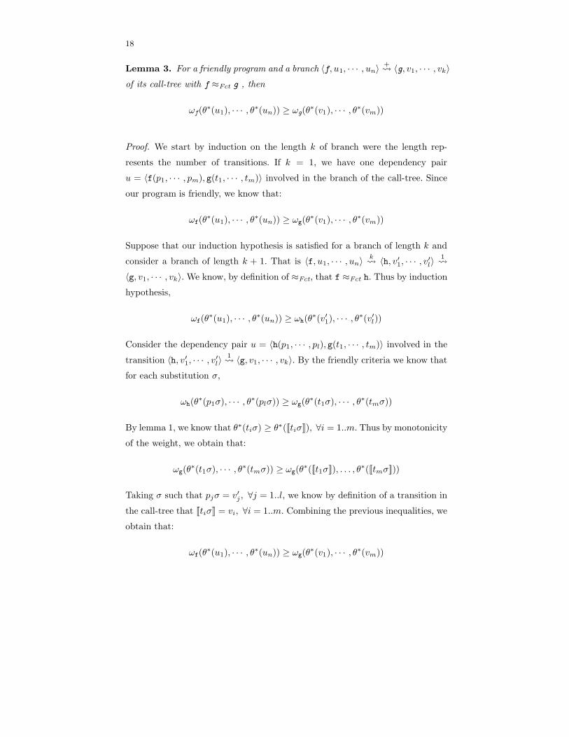
Lemma 3. For a friendly program and a branch 〈f, u1, · · · , un〉+ 〈g, v1, · · · , vk〉

of its call-tree with f ≈Fct g , then

ωf(θ∗(u1), · · · , θ

∗(un)) ≥ ωg(θ∗(v1), · · · , θ

∗(vm))

Proof. We start by induction on the length k of branch were the length rep-

resents the number of transitions. If k = 1, we have one dependency pair

u = 〈f(p1, · · · , pm), g(t1, · · · , tm)〉 involved in the branch of the call-tree. Since

our program is friendly, we know that:

ωf(θ∗(u1), · · · , θ

∗(un)) ≥ ωg(θ∗(v1), · · · , θ

∗(vm))

Suppose that our induction hypothesis is satisfied for a branch of length k and

consider a branch of length k + 1. That is 〈f, u1, · · · , un〉k 〈h, v′1, · · · , v

′l〉

1

〈g, v1, · · · , vk〉. We know, by definition of ≈Fct, that f ≈Fct h. Thus by induction

hypothesis,

ωf(θ∗(u1), · · · , θ

∗(un)) ≥ ωh(θ∗(v′1), · · · , θ

∗(v′l))

Consider the dependency pair u = 〈h(p1, · · · , pl), g(t1, · · · , tm)〉 involved in the

transition 〈h, v′1, · · · , v

′l〉

1 〈g, v1, · · · , vk〉. By the friendly criteria we know that

for each substitution σ,

ωh(θ∗(p1σ), · · · , θ∗(plσ)) ≥ ωg(θ

∗(t1σ), · · · , θ∗(tmσ))

By lemma 1, we know that θ∗(tiσ) ≥ θ∗(JtiσK), ∀i = 1..m. Thus by monotonicity

of the weight, we obtain that:

ωg(θ∗(t1σ), · · · , θ∗(tmσ)) ≥ ωg(θ

∗(Jt1σK), . . . , θ∗(JtmσK))

Taking σ such that pjσ = v′j , ∀j = 1..l, we know by definition of a transition in

the call-tree that JtiσK = vi, ∀i = 1..m. Combining the previous inequalities, we

obtain that:

ωf(θ∗(u1), · · · , θ

∗(un)) ≥ ωg(θ∗(v1), · · · , θ

∗(vm))

19

Lemma 4. Assume that p is a friendly program. For every node 〈g, v1, · · · , vk〉

of the call-tree of root 〈f, u1, · · · , un〉, if g ≈Fct f then

|vj | ≤ ωf(θ∗(u1), · · · , θ

∗(un))

Proof. Since our program is friendly and g ≈Fct f and by lemma 3,

ωf(θ∗(u1), · · · , θ

∗(un)) ≥ ωg(θ∗(v1), · · · , θ

∗(vk))

By subterm property of weight and definition of sup-interpretations,

ωg(θ∗(v1), · · · , θ

∗(vk)) ≥ θ∗(vj) ≥ |vj |, ∀j = 1..k

A.2 Proof of theorem 1

Theorem 1. Assume that p is a friendly program. For each function symbol f

of p there is a polynomial P such that for every value v1, . . . , vn,

‖f(v1, . . . , vn)‖ ≤ P (max(|v1|, ..., |vn|))

A.2.1 Assignments of function symbols

All along, we consider a friendly program p which admits a sup-interpretation.

We now provide an assignment Pf to each function symbol f of a program p,

which is a function bounded by a polynomial and which satisfies that for every

value v1, . . . , vn of Values ,

‖f(v1, . . . , vn)‖ ≤ Pf(max(θ∗(v1), ..., θ∗(vn)))

The assignation is built recursively following the function symbol precedence

≥Fct and on the definition size.

1. Suppose that the definition f(x1, · · · , xn) = ef contains only constructors,

operators or symbols of rank strictly lower that the rank of f wrt ≥Fct.370

We put Pf(X) = θ∗(ef)[X1 ← X, . . . , Xn ← X ]. We write θ∗(ef)[X1 ←

X, . . . , Xn ← X ] to mean that we replace X1, . . . , Xn by the variable X .

20

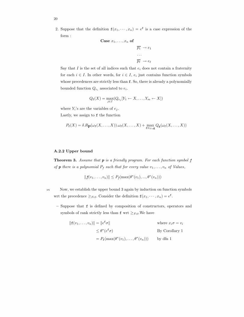
2. Suppose that the definition f(x1, · · · , xn) = ef is a case expression of the

form :

Case x1, . . . , xn of

p1 → e1

. . .

p` → e`

Say that I is the set of all indices such that ei does not contain a fraternity

for each i ∈ I . In other words, for i ∈ I , ei just contains function symbols

whose precedences are strictly less than f. So, there is already a polynomially

bounded function Qeiassociated to ei.

Qf(X) = maxj∈I

(Qej[Y1 ← X, . . . , Ym ← X ])

where Yi’s are the variables of ej .

Lastly, we assign to f the function

Pf(X) = δ.Rp(ωf(X, . . . , X)).ωf(X, . . . , X) + maxf≈Fctg

Qg(ωf(X, . . . , X))

A.2.2 Upper bound

Theorem 3. Assume that p is a friendly program. For each function symbol f

of p there is a polynomial Pf such that for every value v1, . . . , vn of Values,

‖f(v1, . . . , vn)‖ ≤ Pf(max(θ∗(v1), ..., θ∗(vn)))

Now, we establish the upper bound 3 again by induction on function symbols375

wrt the precedence ≥Fct. Consider the definition f(x1, · · · , xn) = ef.

– Suppose that f is defined by composition of constructors, operators and

symbols of rank strictly less than f wrt ≥Fct.We have

‖f(v1, . . . , vn)‖ = ‖efσ‖ where xiσ = vi

≤ θ∗(efσ) By Corollary 1

= Pf(max(θ∗(v1), . . . , θ∗(vn))) by dfn 1

21

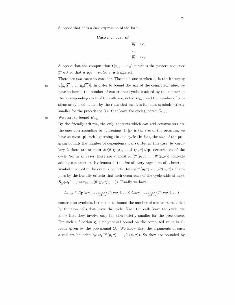
– Suppose that ef is a case expression of the form.

Case x1, . . . , xn of

p1 → e1

. . .

p` → e`

Suppose that the computation f(v1, . . . , vn) matches the pattern sequence

pi wrt σ, that is piσ = vi. So ei is triggered.

There are two cases to consider. The main one is when ei is the fraternity

C[g1(t1), . . . , gr(tr)]. In order to bound the size of the computed value, we380

have to bound the number of constructor symbols added by the context in

the corresponding cycle of the call-tree, noted E≈Fctand the number of con-

structor symbols added by the rules that involves function symbols strictly

smaller for the precedence (i.e. that leave the cycle), noted E>Fct.

We start to bound E≈Fct:385

By the friendly criteria, the only contexts which can add constructors are

the ones corresponding to lightenings. If |p| is the size of the program, we

have at most |p| such lightenings in one cycle (In fact, the size of the pro-

gram bounds the number of dependency pairs). But in this case, by corol-

lary 2 there are at most δω(θ∗(p1σ), . . . , θ∗(pnσ))/|p| occurrences of the

cycle. So, in all cases, there are at most δω(θ∗(p1σ), . . . , θ∗(pnσ)) contexts

adding constructors. By lemma 4, the size of every argument of a function

symbol involved in the cycle is bounded by ωf(θ∗(p1σ), · · · , θ∗(pnσ)). It im-

plies by the friendly criteria that each occurrence of the cycle adds at most

Rp(ωf(. . . , maxi=1..n(θ∗(piσ)), . . .)). Finally we have:

E≈Fct≤ Rp(ωf(. . . , max

i=1..n(θ∗(piσ)), . . .)).δuωf(. . . , max

i=1..n(θ∗(piσ)), . . .)

constructor symbols. It remains to bound the number of constructors added

by function calls that leave the cycle. Since the calls leave the cycle, we

know that they involve only function strictly smaller for the precedence.

For such a function g, a polynomial bound on the computed value is al-

ready given by the polynomial Qg. We know that the arguments of such

a call are bounded by ωf(θ∗(p1σ), · · · , θ∗(pnσ)). So they are bounded by

22

ωf(. . . , maxi=1..n(θ∗(piσ)), . . .). So the number of constructor symbols added

by such a call is bounded by Qg(ωf(. . . , maxi=1..n(θ∗(piσ)), . . .)). Finally,

since the sup-interpretations of contexts oblige to take the maximum of such

calls, we have:

E>Fct≤ max

g≈Fctf(Qg(ωf(. . . , max

i=1..n(θ∗(piσ)), . . .)))

So we have:

‖f(v1, · · · , vn)‖ = E>Fct+ E≈Fct

≤ Pf( maxi=1..n

(θ∗(piσ)))

Lastly, if ei is not a fraternity. Then we have already a bound Qf on the size

of the computed value. Thus

‖f(v1, · · · , vn)‖ ≤ Qf(ωf(. . . , maxi=1..n

(θ∗(piσ)), . . .))

≤ Pf( maxi=1..n

(θ∗(piσ)))

Thus proving theorem 3. Finally, we have:

‖f(v1, · · · , vn)‖ ≤ Pf( maxi=1..n

(θ∗(vi))) by theorem 3

≤ Pf( maxi=1..n

(α(|vi|))) by lemma 2

≤ Pf(α( maxi=1..n

(|vi|)))

Thus proving theorem 1.

A.3 Proof of theorem 2

We first begin by proving the following lemma and then we define a notion of

rank:

Lemma 5. Given a friendly program, for every rule of the shape f(p1, · · · , pn)→

C[e] and every subsitution σ, there is a polynomial Q such that:

‖eσ‖ ≤ Q( maxi=1..n

(|piσ|))

23

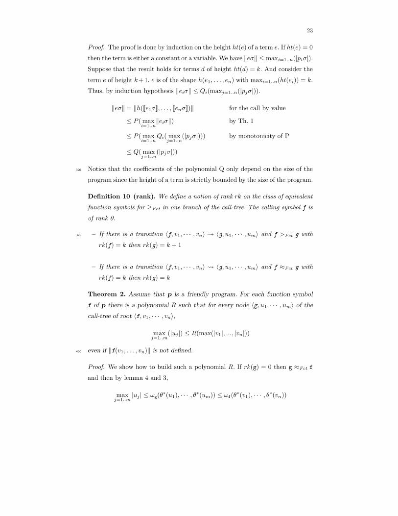
Proof. The proof is done by induction on the height ht(e) of a term e. If ht(e) = 0

then the term is either a constant or a variable. We have ‖eσ‖ ≤ maxi=1..n(|piσ|).

Suppose that the result holds for terms d of height ht(d) = k. And consider the

term e of height k+1. e is of the shape h(e1, . . . , en) with maxi=1..n(ht(ei)) = k.

Thus, by induction hypothesis ‖eiσ‖ ≤ Qi(maxj=1..n(|pjσ|)).

‖eσ‖ = ‖h(Je1σK, . . . , JenσK)‖ for the call by value

≤ P ( maxi=1..n

‖eiσ‖) by Th. 1

≤ P ( maxi=1..n

Qi( maxj=1..n

(|pjσ|))) by monotonicity of P

≤ Q( maxj=1..n

(|pjσ|))

Notice that the coefficients of the polynomial Q only depend on the size of the390

program since the height of a term is strictly bounded by the size of the program.

Definition 10 (rank). We define a notion of rank rk on the class of equivalent

function symbols for ≥Fct in one branch of the call-tree. The calling symbol f is

of rank 0.

– If there is a transition 〈f, v1, · · · , vn〉 〈g, u1, · · · , um〉 and f >Fct g with395

rk(f) = k then rk(g) = k + 1

– If there is a transition 〈f, v1, · · · , vn〉 〈g, u1, · · · , um〉 and f ≈Fct g with

rk(f) = k then rk(g) = k

Theorem 2. Assume that p is a friendly program. For each function symbol

f of p there is a polynomial R such that for every node 〈g, u1, · · · , um〉 of the

call-tree of root 〈f, v1, · · · , vn〉,

maxj=1..m

(|uj |) ≤ R(max(|v1|, ..., |vn|))

even if ‖f(v1, . . . , vn)‖ is not defined.400

Proof. We show how to build such a polynomial R. If rk(g) = 0 then g ≈Fct f

and then by lemma 4 and 3,

maxj=1..m

|uj | ≤ ωg(θ∗(u1), · · · , θ

∗(um)) ≤ ωf(θ∗(v1), · · · , θ

∗(vn))

24

Taking R0(X) = ωf(α(X), . . . , α(X)) we obtain the required polynomial bound.

Suppose that we have built a polynomial Rk for the function symbols of rank k

and that rk(g) = k + 1. There is a dependency pair 〈f1(q1, · · · , ql),

g1(s1, · · · , sl′)〉 involved in the branch 〈f, v1, · · · , vn〉+ 〈g, u1, · · · , um〉 of the

call-tree, for a given substitution σ, and such that rk(f1) = k and rk(g1) = k+1

(i.e. g ≈Fct g1). We know that maxi=1..l |qiσ| ≤ Rk(max(|v1|, ..., |vn|)).

maxi=1..m

|ui| ≤ ωg1(θ∗(Js1σK), . . . , θ∗(Jsl′σK)) by lemma 4

≤ ωg1(α( max

i=1..n‖siσ‖), . . . , α( max

i=1..n‖siσ‖)) by lemma 2

≤ ωg1(. . . , α(Q(max

i=1..l|qiσ|)), . . .) by lemma 5

≤ ωg1(. . . , α(Q(Rk( max

j=1..n|vj |))), . . .) by lemma I.H.

Then we put Rk+1(X) = max(Rk(X), ωg1(. . . , α(Q(Rk(X))), . . .). Finally, for

the highest rank l we put R(X) = Rl(X). Such a l exists since the rank is

bounded by the number of function symbols and consequently by the size of the

program |p|. Consequently, the polynomial is independant of the inputs. Now

we prove by induction on the rank that for every k Rk gives a bound on the

size of the values belonging to states whose rank of function symbol is smaller

than k. We have shown that it is true for k = 0. Suppose that it is true for k.

By construction and induction hypothesis, Rk+1 bounds the values of the states

of rank smaller or equal to k. Given a state 〈h, w1, · · · , wl′〉 of the branch with

rk(h) = k + 1 (i.e. h ≈Fct g1).

maxi=1..l′

|wi| ≤ ωg1(θ∗(Js1σK), . . . , θ∗(JsmσK)) by lemma 7

≤ ωg1(. . . , α(Q(Rk( max

j=1..n|vj |))), . . .) cf. above

≤ Rk+1( maxj=1..n

|vj |) by construction of Rk+1

Finally R gives a bound on the size of every value of the call-tree, even if the call-

tree is infinite (In this case, the program is non-terminating and it adds at least

an infinite branch of states whose respective function symbols are equivalent for

the precedence ≥Fct).

25

B Examples405

Definition 11 (Dependency pairs graph). Let DP(p) be the set of all de-

pendency pairs of a program p. The dependency pair graph DPG(p) of a program

is defined by

– The set of nodes is DP(p).

– There is an edge between410

〈f(p1, · · · , pn), g(t1, · · · , tm)〉 and 〈g(q1, · · · , qm), h(s1, · · · , sk)〉.

The notion of dependency pairs graph is useful in order to have a clearest view

of programs. In fact, the call-tree of a program is no more than an unfolding of

the dependency pair graph.

Example 6. Consider the program for multiplication:

mult(x, y) = Case x, y of 0, u→ 0

S(z), u→ add(u, mult(z, u)))

add(x, y) = Case x, y of S(u),0→ S(u)

0,S(v)→ S(v)

S(u),S(v)→ S(S(add(u, v)))

We define the sup-interpretation θ by taking θ(add)(X, Y ) = X+Y and θ(S)(X) =415

X+1. The program owns two fraternities add(y, [mult(z, u)])) and S(S[add(u, v)])

called respectively by mult(S(z), u) and add(S(u),S(v)). By taking ωadd(X, Y ) =

ωmult(X, Y ) = X+Y , the inequalities of the friendly criteria are strictly statisfied

for every subsitution σ. So it remains to check the context’s sup-interpretations.

Since θ∗(S(S(�))) = � + 2 and θ∗(add(y, �))) = � + θ∗(y) = � + Y , pmult is a420

friendly program. This example illustrates an interesting case where the polyno-

mial R(X) = X added by the contexts and defined in the friendly criteria is no

longer a constant.

26

Example 7. Consider the program for exponential:

exp(x) = Case x of 0→ S(0)

S(y)→ double(exp(y))

double(x) = Case x of 0→ 0

S(y)→ S(S(double(y)))

θ(double)(X) is at least equal to 2X and the program contains a fraternity

involving double in its context. Consequently, the program pexp is not friendly.425

Example 8. The following program computes the greatest common divisor:

minus(x, y) = Case x, y of 0, z → 0

S(z),0→ S(z)

S(u),S(v)→ minus(u, v)

le(x, y) = Case x, y of 0, z → True

S(z),0→ False

S(u),S(v)→ le(u, v)

if(x, y, z) = Case x, y, z of True, u, v → u

False, u, v → v

gcd(x, y) = Case x, y of 0, z → z

S(z),0→ S(z)

S(u),S(v)→ if(le(u, v), gcd(minus(v, u),S(u)),gcd(minus(u, v),S(v)))

This program admits four cycles: two depending on minus and le which verify

the friendly criteria and two other on the gcd function. Since the corresponding

context to these latter cycles is the function if whose sup-interpretation can be

taken to be max, and by taking θ(S)(X) = X + 1, we only have to check that,

there exist θ and ω such that:

ωgcd(U + 1, V + 1) ≥ ωgcd(θ(minus)(V, U), U + 1)

ωgcd(V + 1, V + 1) ≥ ωgcd(θ(minus)(U, V ), V + 1)

27

We can take θ(minus)(X, Y ) equal to X and ωgcd(X, Y ) = X + Y so that the

previous inequalities are satisfied over reals, consequently also on substitutions’

sup-interpretation and the program is friendly.

Example 9. The following program eliminates duplicates from a list:

equi(x, y) = Case x, y of 0,0→ True

0,S(v)→ False

S(u),0→ True

S(u),S(v)→ equi(u, v)

remove(x, y) = Case x, y of n,nil→ nil

n, c(m, l)→ if(equi(n, m), n, c(m, l))

if(x, y, z) = Case x, y, z of True, n, c(m, l)→ remove(n, l)

False, n, c(m, l)→ c(m, remove(n, l))

elim(x) = Case x of nil→ nil

c(n, l)→ c(n, elim(remove(n, l)))

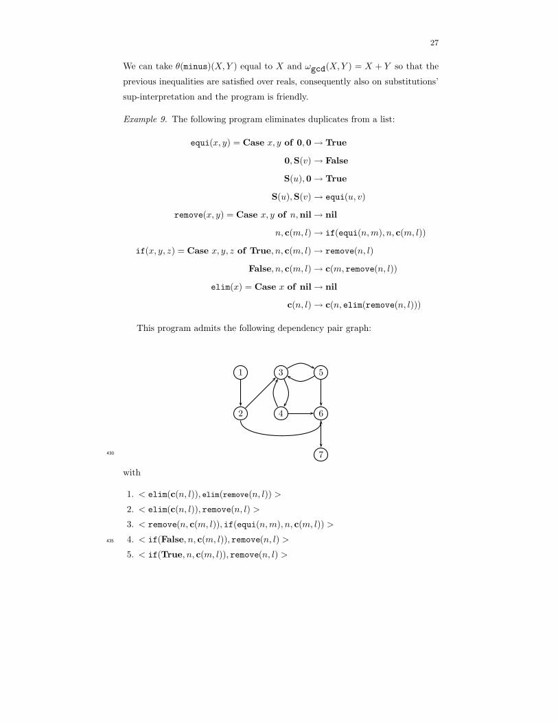
This program admits the following dependency pair graph:

1 3 5

2 4 6

7430

with

1. < elim(c(n, l)), elim(remove(n, l)) >

2. < elim(c(n, l)), remove(n, l) >

3. < remove(n, c(m, l)), if(equi(n, m), n, c(m, l)) >

4. < if(False, n, c(m, l)), remove(n, l) >435

5. < if(True, n, c(m, l)), remove(n, l) >

28

6. < remove(n, c(m, l)), equi(n, m) >

7. < equi(S(u),S(v)), equi(u, v) >

So the precedence holds as follows elim >Fct remove ≈Fct if >Fct equi. Now

we want to check the constraint on recursive calls. There are four cycles in the440

graph and we want to find ω and θ such that:

∀σ, ωelim(θ∗(c(n, l)σ)) ≥ ωelim(θ∗(remove(n, l)σ))

∀σ, ωequi(θ∗(S(u)σ), θ∗(S(v)σ)) ≥ ωequi(θ∗(uσ), θ∗(vσ))

∀σ, ωremove(θ∗(nσ), θ∗(c(m, l)σ)) ≥ ωif(θ∗(equi(n, m)σ), θ∗(nσ), θ∗(c(m, l)σ))

∀σ, ωif(θ∗(False), θ∗(nσ), θ∗(c(m, l)σ)) ≥ ωremove(θ∗(nσ), θ∗(lσ))445

∀σ, ωif(θ∗(True), θ∗(nσ), θ∗(c(m, l)σ)) ≥ ωremove(θ∗(nσ), θ∗(lσ))

We take ωelim as the identity and ω =∑

otherwise. It remains to prove

that :

1. ∀σ, θ∗(c(n, l)σ) ≥ θ∗(remove(n, l)σ)

2. ∀σ, θ∗(S(u)σ) + θ∗(S(v)σ) ≥ θ∗(uσ) + θ∗(vσ)450

3. ∀σ, θ∗(nσ) + θ∗(c(m, l)σ) ≥ θ∗(equi(n, m)σ) + θ∗(nσ) + θ∗(c(m, l)σ)

4. ∀σ, θ∗(False) + θ∗(nσ) + θ∗(c(m, l)σ) ≥ θ∗(nσ) + θ∗(lσ)

5. ∀σ, θ∗(True) + θ∗(nσ) + θ∗(c(m, l)σ) ≥ θ∗(nσ) + θ∗(lσ)

Inequalities 2, 4 and 5 are strict since True, False, S and c are constructors of

respective arities 0, 0, 1 and 2. For inequality 1, we take θ∗(remove(n, l)) = L455

since the result of the remove function is a list smaller than the input one. So

inequality 1 is strictly satisfied. Finaly, we can take θ(equi(n, m)) = 0 since the

result is a constructor of arity 0. As a result, the third constraint becomes an

equality and is satisfied.

Now, consider the following definitions included in the program:

remove(n, c(m, l)) = if(equi(n, m), n, c(m, l))

if(True, n, c(m, l)) = remove(n, l)

if(False, n, c(m, l)) = c(m, remove(n, l))

Since if ≈Fct remove, the three respective fraternities have the following con-460

texts C1[�] = �, C2[�] = � and C3[�] = c(m, �). θ(C3[�]) = � + M + 1 =

29

max(�+ R(M)) with R = M + 1 and θ∗(m) = M . Since the corresponding in-

equality is strict our program is friendly. Finally, as a consequence of theorem 1,

there exist Pelim such that for every value v1:‖elim(v1)‖ ≤ Pelim(|v1|)

Example 10. The following program computes the reachability problem for graphs:

equi(x, y) = Case x, y of

0,0→ True

0,S(z)→ False

S(z),0→ False

S(u),S(v)→ equi(u, v)

or(x, y) = Case x, y of

True, y → True

False, y → False

union(x, y) = Case x, y of

ε, h→ h

edge(x, y, i), h→ edge(x, y, union(i, h))

reach(x, y, z, u) = Case x, y, z, u of

x, y, ε, h→ False

x, y, edge(u, v, i), h→ if1(equi(x, u), x, y, edge(u, v, i), h)

if1(x, y, z, u, v) = Case x, y, z, u, v of

True, x, y, edge(u, v, i), h→ if2(equi(y, v), x, y, edge(u, v, i), h)

False, x, y, edge(u, v, i), h→ reach(x, y, i, edge(u, v, h))

if2(x, y, z, u) = Case x, y, z, u of

True, x, y, edge(u, v, i), h→ true

False, x, y, edge(u, v, i), h→ or(reach(x, y, i, h),

reach(v, y, union(i, h), ε))

Here is the corresponding dependency graph (without the equi and union func-465

tion symbols):

30

1

2 3

4 5

with the nodes corresponding to the following dependency pairs:

1. < reach(x, y, edge(u, v, i), h), if1(equi(x, u), x, y, edge(u, v, i), h) >470

2. < if1(True, x, y, edge(u, v, i), h), if2(equi(y, v), x, y, edge(u, v, i), h)) >

3. < if1(False, x, y, edge(u, v, i), h), reach(x, y, i, edge(u, v, h)) >

4. < if2(True, x, y, edge(u, v, i), h), reach(x, y, i, h) >

5. < if2(True, x, y, edge(u, v, i), h), reach(x, y, i, h) >

We can see that the graph is composed of 3 smallest cycles. Since each de-

pendency pair involve empty contexts or the or function symbol whose sup-

interpretation can clearly be taken to be the maximum of its inputs, we only

have to check non strict inequalities to ensure the friendly criteria. Since the

equi function symbol only returns booleans, we can take its sup-interpretation

to be null. The sup-interpretation of the edge constructor can be assimilated

to the size of the value. It remains to find a sup-interpretation θ and a weight

ω such that(if the inequalities are satisfied over reals, they are also satisfied for

every sup-interpretation of a substitution of a variable):

ωreach(X, Y, U + V + I + 1, H) ≥ ωif1(0, X, Y, U + V + I + 1, H)

ωif1(0, X, Y, U + V + I + 1, H) ≥ ωif2

(0, X, Y, U + V + I + 1, H)

ωif2(0, X, Y, U + V + I + 1, H) ≥ ωreach(X, Y, I, H)

ωif2(0, X, Y, U + V + I + 1, H) ≥ ωreach(V, Y, θ(union)(I, H), 0)

ωif1(0, X, Y, U + V + I + 1, H) ≥ ωreach(X, Y, I, H + U + V + 1)

Since the function symbol union makes the union between two graphs, we can

take its sup-interpretation to be the sum of the size of the two graphs. FinalLy,

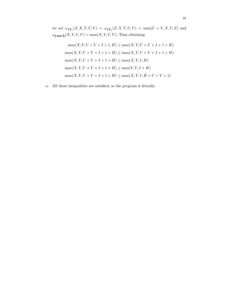
31

we set ωif1(Z, X, Y, U, V ) = ωif2

(Z, X, Y, U, V ) = max(U + V, X, Y, Z) and

ωreach(X, Y, U, V ) = max(X, Y, U, V ). Thus obtaining:

max(X, Y, U + V + I + 1, H) ≥ max(X, Y, U + V + I + 1 + H)

max(X, Y, U + V + I + 1 + H) ≥ max(X, Y, U + V + I + 1 + H)

max(X, Y, U + V + I + 1 + H) ≥ max(X, Y, I, H)

max(X, Y, U + V + I + 1 + H) ≥ max(V, Y, I + H)

max(X, Y, U + V + I + 1 + H) ≥ max(X, Y, I, H + U + V + 1)

All these inequalities are satisfied, so the program is friendly.475

32

C A termination criteria

In this section, using definitions and lemmas introduced in appendix A.1, we

prove that the friendly criteria can be used to prove termination of programs.

Lemma 6. For a friendly program and a branch 〈f, u1, · · · , un〉+ 〈g, v1, · · · , vk〉

of its call-tree with f ≈Fct g involving a lightening , then

ωf(θ∗(u1), · · · , θ

∗(un)) ≥ 1/δ + ωg(θ∗(v1), · · · , θ

∗(vm))

Proof. Suppose that lightening u = 〈h(p1, · · · , pl), h’(t1, · · · , tl′)〉 corresponding

to 〈h, v′1, · · · , v′l〉

C[�] 〈h, w1, · · · , wl′ 〉 is involved in the branch of the call-tree,

with wj = JtjσK and piσ = v′i for a given subsitution σ, then by the friendly

criteria:

ωh(θ∗(p1σ), · · · , θ∗(plσ)) ≥ 1/δu + ωh’(θ

∗(t1σ), · · · , θ∗(tl′σ))

≥ 1/δu + ωh’(θ∗(w1), · · · , θ

∗(wl′ ))

ωh(θ∗(v′1), · · · , θ

∗(v′l)) ≥ 1/δ + ωh’(θ∗(w1), · · · , θ

∗(wl′)) by Dfn of δ

By lemma 3, we have

ωf(θ∗(u1), · · · , θ

∗(un)) ≥ ωh(θ∗(v′1), · · · , θ

∗(v′l))

and

ωh’(θ∗(w1), · · · , θ

∗(wl′ )) ≥ ωg(θ∗(v1), · · · , θ

∗(vm))

Finally,

ωf(θ∗(u1), · · · , θ

∗(un)) ≥ 1/δ + ωg(θ∗(v1), · · · , θ

∗(vm))

Lemma 7. Given a subsitution σ, suppose that we have a cycle in the evaluation

of f starting from 〈f, p1σ, · · · , pnσ〉 in the call-tree of a friendly program. If there480

is a lightening u = 〈g(q1, · · · , qm), h(s1, · · · , sk)〉 involved in this cycle then there

are at most δω(θ∗(p1σ), . . . , θ∗(pnσ)) occurrences of the cycle in the call-tree.

Proof. The proof is based on lemma 6. If we have a lightening involved in a cycle,

we know that we decrease ω(θ∗(p1σ), . . . , θ∗(pnσ)) by at least 1/δ for each oc-

currence of a cycle. Thus we have at most δω(θ∗(p1σ), . . . , θ∗(pnσ)) occurrences.485

33

Corollary 2. If k lightenings are involved in a cycle of the call-tree of a friendly

program, then there are at most δω(θ∗(p1σ), . . . , θ∗(pnσ))/k occurrences of the

cycle in the call-tree.

Theorem 4. If the program is friendly and such that each cycle in its call-tree

involved a lightening, then the program is terminating.490

Proof. There are no infinite loops in the program since we bound the number of

occurrences of each cycle. Thus it terminates.

Remark 2. Notice that a version of previous theorem could also be applied to

non-friendly programs such as exponential in example 7 of appendix A.1, if we

forget the condition on sup-interpretation of contexts. In the case of exponential,

we have to check the following inequalities:

∀σ, ωdouble(θ∗(S(xσ))) > ωdouble(θ

∗(xσ))

∀σ, ωexp(θ∗(S(xσ))) > ωexp(θ

∗(xσ))

This is done by taking ωdouble(X) = ωexp(X) = X so that exp is also terminating.