resource allocation in wireless ad-hoc networksmaximuswang.com/paper/mscthesis.pdfdepartment of...
TRANSCRIPT
DEPARTMENT OF ELECTRICAL AND ELECTRONIC ENGINEERING
COMMUNICATION AND SIGNAL PROCESSING
Resource Allocation in Wireless Ad-Hoc
Networks
Xiaoqin Wang
Master Thesis
September 2011
Supervisor: Dr. Mustafa Gurcan
2
Abstract
A wireless Ad-Hoc network is an infrastructure-less communication networks without any
central administrations, in which nodes communicate with each other utilizing multi-hop
wireless links. Intermediate nodes between a pair of nodes that are not in the transmission
range of each other act as relays. However, the intermediate nodes along the multi-hop path
can drain the battery power of nodes quickly. Therefore, the resource allocation plays a very
significant role in dealing with the energy constraint in wireless Ad-Hoc networks. This
thesis studies channel-aware resource allocation schemes for High Speed Downlink Packet
Access (HSDPA) systems and focuses on the cross-layer resource allocation schemes in
wireless Ad-Hoc networks which adopt HSDPA system for communication on each wireless
link.
This thesis addresses the problem of the residual transmission energy in HSDPA systems at
the physical layer. And a two-group resource allocation scheme is introduced to improve the
residual energy utilization. This proposed scheme is examined can achieved a higher data rate
than the data rate achieved with the current HSDPA type of algorithm in both interference-
free and interference-present environments.
After the transmission power and the data rates are defined as the cost function of the routing
scheme, several energy-ware routing path discovery schemes are proposed to find the routing
path with the minimum energy consumption. And a novel energy-aware routing path
discovery scheme is developed to reduce the computational complexity. As the two-group
resource allocation scheme can further reduce the energy consumption per bit for
transmission on each path, the data bits can be assigned to each path in such a way that the
total energy consumed is minimized. And then, the MAC distributed coordination function
(DCF) service time is studied, and the end-to-end delay time of the paths adopting different
resource allocation schemes are determined.
Finally, this thesis studies the coded parity packet (CPP) scheme which can decrease the
packet error rate and reduce the number of re-transmissions. After the performance of the
CPP approach in wireless Ad-Hoc networks is analysed, an adaptable transmission
mechanism is developed in this thesis by using CPP scheme to achieve the energy efficiency
transmission in wireless Ad-Hoc networks.

3
Contents
Abstract ................................................................................................................ 2
Contents ............................................................................................................... 3
List of Figures ...................................................................................................... 5
Abbreviations and Acronyms ............................................................................ 7
List of Notation .................................................................................................... 8
Acknowledgements.............................................................................................. 9
Chapter 1............................................................................................................ 10
1.1 Wireless Ad-Hoc Networks ....................................................................................... 10
1.2 Routing Protocols in Wireless Ad-Hoc Networks ..................................................... 11
1.3 Propagation Models ................................................................................................... 12
1.3.1 Free Space Propagation Model ..................................................................................... 13
1.3.2 Two-Ray Ground Reflection Model ............................................................................... 13
1.4 HSDPA Overview ..................................................................................................... 13
1.5 Thesis Outline ............................................................................................................ 15
Chapter 2............................................................................................................ 16
2.1 Introduction ................................................................................................................ 16
2.2 High-Speed Downlink Packet Access (HSDPA) System .......................................... 16
2.2.1 Signal Processing at the Transmitter ............................................................................. 17
2.2.2 Radio Channel ............................................................................................................... 17
2.2.3 Signal Processing at the Receiver ................................................................................. 18
2.3 Rate Allocation in HSDPA Systems.......................................................................... 18
2.3.1 Equal Energy and Equal Rate Allocation in HSDPA Systems ..................................... 19
2.3.2 Residual Energy Utilization .......................................................................................... 20
2.3.3 Two-group Resource Allocation Scheme ..................................................................... 21
2.3.4 Resource Allocation in Frequency Selective Channels................................................. 22
2.4 MAC DCF Working Process ..................................................................................... 26
2.5 MAC DCF Service Time ........................................................................................... 28
4
2.5.1 Successful Frame Reception Probability ...................................................................... 28
2.5.2 Scheduling Probability .................................................................................................. 29
2.5.3 Modelling the IEEE 802.11 DCF .................................................................................. 31
2.6 Simulation and Performance Evaluation ................................................................... 32
Chapter 3............................................................................................................ 39
3.1 Introduction ................................................................................................................ 39
3.2 Minimization of Energy Consumption Per Bit .......................................................... 39
3.3 The Trellis-hop Diagram Routing Discovery Scheme .............................................. 41
3.4 Modified Viterbi Algorithm ...................................................................................... 43
3.5 Modified Floyd Algorithm ........................................................................................ 47
3.6 Performance Evaluation ............................................................................................. 54
Chapter 4............................................................................................................ 56
4.1 Introduction ................................................................................................................ 56
4.2 System Overview ....................................................................................................... 56
4.3 Channel Encoder ........................................................................................................ 57
4.3.1 The Outer Encoder ........................................................................................................ 58
4.3.2 The Inner Encoder ......................................................................................................... 59
4.4 Channel Decoder ....................................................................................................... 60
4.5 Performance Analysis of CPP Approach in Wireless Ad-Hoc Networks ................. 64
4.5.1 Basic Retransmission Schemes ..................................................................................... 65
4.5.2 Transmission with CPP Approach ................................................................................ 66
4.5.3 Transmission with Adjustable Power............................................................................ 67
4.5.4 An Adaptable Transmission Mechanism in Wireless Ad-Hoc Networks ..................... 68
4.6 Simulation and Performance Evaluation ................................................................... 69
Chapter 5............................................................................................................ 73
5.1 Thesis Summary ........................................................................................................ 73
5.2 Future Work ............................................................................................................... 74
REFERENCE .................................................................................................... 76

5
List of Figures
Figure 1.1 A Wireless Ad-Hoc Network ................................................................................. 11
Figure 2.1 Signal processing and transmission in discrete time and continuous time domains
for a single sub-channel ........................................................................................................... 17
Figure 2.2 HSDPA System Structure....................................................................................... 19
Figure 2.3 Procedure of bit channel loading for the Two Group algorithm ............................ 21
Figure 2.4 DCF Transmission .................................................................................................. 27
Figure 2.5 The data rate realized by different resource allocation schemes ............................ 33
Figure 2.6 System capacity and bit rate achieved by One-group HSDPA system and Two-
group HSDPA system as a function of distance ...................................................................... 34
Figure 2.7 System capacity and bit rate achieved by One-group HSDPA system and Two-
group HSDPA system as a function of SNR ........................................................................... 35
Figure 2.8 Network Topology.................................................................................................. 36
Figure 2.9 Network Topology with Disjoint Multiple Routing Paths ..................................... 37
Figure 2.10 End-to-end delay predicted from equation (2.50) ................................................ 38
Figure 3.1 A 5-node Network Topology .................................................................................. 42
Figure 3.2 The First Neighbour of Source Node for Trellis-hop Diagram .............................. 42
Figure 3.3 The Second Neighbour of Source Node for Trellis-hop Diagram ......................... 43
Figure 3.4 The Third Neighbour of Source Node for Trellis-hop Diagram ............................ 43
Figure 3.5 The First Hop Level for Routing Paths Discovery ................................................. 45
Figure 3.6 The Second Hop Level for Routing Paths Discovery ............................................ 46
Figure 3.7 The Third Hop Level for Routing Paths Discovery ............................................... 46
Figure 3.8 The Forth Hop Level for Routing Paths Discovery................................................ 46
Figure 3.9 Disjoint Multiple Routing Discoveries ................................................................... 54

6
Figure 4.1 The Coded Parity Packets Approach Model .......................................................... 57
Figure 4.2 The process of the external extrinsic LLR generation [23] .................................... 62
Figure 4.3 Flow chart of the adaptable transmission mechanism ............................................ 69
Figure 4.4 The packet error rate for the first set of CPP code rates ......................................... 70
Figure 4.5 The packet error rate of the second set of the CPP code rates ............................... 71

7
Abbreviations and Acronyms
CDMA Code Division Multiple Access
UMTS Universal Mobile Telecommunications System
WCDMA Wideband Code Division Multiple Access
DS-CDMA Direct-Sequence Code Division Multiple Access
QoS Quality of Service
HSDPA High Speed Downlink Packet Access
3GPP 3rd Generation Partnership Project
DSDV Destination-Sequenced Distance-Vector Routing
OLSR Optimized link-state routing protocol
AODV Ad hoc On-Demand Distance Vector Routing
DSR Dynamic Source Routing
TORA Temporally-Ordered Routing Algorithm
SENCAST Scalable Protocol for Unicasting and Multicasting in a Large Ad hoc
Emergency Network
RREQ Route request packet
AMC Adaptive Modulation and Coding
QAM Quadratic Amplitude Modulation
SINR Signal to Interference plus Noise Ratio
ISI Inter Symbol Interference
MMSE Minimum Mean Square Error
SIC Successive Interference Cancellation
LLR Logarithm of the likelihood ratio
MAI Multiple Access Interference

8
List of Notation
Column vector
A Matrix
[A]ij The element of matrix A in row i column j
AH Conjugate transpose of matrix A
AT Transpose of matrix A
A−1
Inverse matrix of matrix A
tr(A) trace of matrix A
A ⊗ B Kronecker product of matrices
Im Identity matrix with size m × m
⌊ ⌋ The largest integer being smaller or equal to x
⌈ ⌉ The smallest integer being larger or equal to x
The diagonal matrix having the elements of vector in main diagonal line

9
Acknowledgements
I here confirm that all the technical contributions presented in this thesis are originated in my
research, and I will take full responsibilities on them. I also confirm that all the work of
others presented in this thesis have been clearly acknowledged and properly cited.
I am most indebted to Dr Mustafa Gurcan, my supervisor, who, in the past few months,
introduced me to the HSDPA system and wireless Ad-Hoc networks. His wide knowledge
and insightful thinking have been of great value for me. I am thankful for his patience and
guidance. It is implausible that I would have seen this endeavour through to its end without
him.
I wish also to express my thanks to Mr Anusorn Chungtragarn who gave me useful help
during many technical discussions in doing this research.
Finally, above all, I wish to thank my parents. They gave me this opportunity of studying
abroad to accept high quality education, and they never ask me to requite for what they have
done in the last 23 years. To them I dedicate this thesis.

1. Introduction
10
Chapter 1
Introduction
Wireless Ad-Hoc networks have been the topic of extensive research for around twenty years.
Due to their inherent distributed nature, ad-hoc networks are more robust than their cellular
counterparts against single-point failure, and have the flexibility to reroute around congested
nodes [1]. With limited energy in each node, how to reduce the energy consumption of nodes
to transmit a certain amount of data becomes a main research area for wireless Ad-Hoc
networks. And the energy consumption is a key design criterion, especially when parallel
channel transmission is adopted in these networks. The current high speed downlink packet
access (HSDPA) systems with multiple parallel channels, which may produce a significant
amount of residual energy for realizing equal data rate per channel, is implemented on
wireless Ad-Hoc networks to achieve higher transmission rates.
1.1 Wireless Ad-Hoc Networks
Wireless networks are traditionally classified into two categories: networks with fixed
infrastructure and Ad-Hoc networks. The former networks usually comprise one or more
centralised nodes which link with the Internet backbone. Mobile nodes can communicate
with the access point performing the key networking and control functions for them. There
are no peer-to-peer communications between mobile nodes in these networks. And all the
mobile nodes can communicate with Internet backbone through the access point by single-
hop routing.
A wireless Ad-Hoc network is a collection of nodes which communicate with each other
by forming a multi-hop radio network with no centralized administration or fixed
infrastructure. The communications between mobile nodes in these networks do not rely on a
centralize station/ pre-existing infrastructure to control or coordinate. The nodes in wireless
Ad-Hoc networks can communicate directly with each other whenever they are within their
transmission ranges and communicate through intermediate nodes using multi-hop routing to

1. Introduction
11
extend their communication ranges and consequently forward their information packets to
other nodes which are out of their transmission ranges [2]. An example of a simple Ad-Hoc
network is shown in Figure 1.1.
The earliest wireless ad-hoc networks were the “packet radio” networks (PRNETs) dating
to the 1970s which is sponsored by DARPA after the ALOHAnet project [3] Wireless Ad hoc
networks have been greatly developed in the last forty years and can be further classified into
three categories: mobile ad hoc networks (MANETs), wireless mesh networks (WMN) and
wireless sensor networks (WSN).
Figure 1.1 A Wireless Ad-Hoc Network
1.2 Routing Protocols in Wireless Ad-Hoc Networks
According to the working principles, the routing protocols in ad-hoc networks can be
classified into two categories, one is active routing protocol, and the other is on-demand
routing protocol. The active routing protocol maintains fresh lists of destinations and their
routes by distributing routing table throughout the network periodically. The typical active
routing protocols are DSDV [4], OLSR [5], etc. On the other hand, the on-demand routing
protocol, which includes AODV [6], DSR [7], SENCAST [8] does not require routing
maintenance. In such protocol, a routing path between the source and the destination is
constructed by route discovery when it is demanded. And the contents of the routing tables
are only a part of the whole topology of the network. AODV is one of the most popular
single-path reactive routing protocols. This protocol establishes route between nodes only as
desired by source node. When the source node wants to send packet to destination, it checks
the local routing table firstly, and then directly sends the packet to it. Otherwise, the route
1. Introduction
12
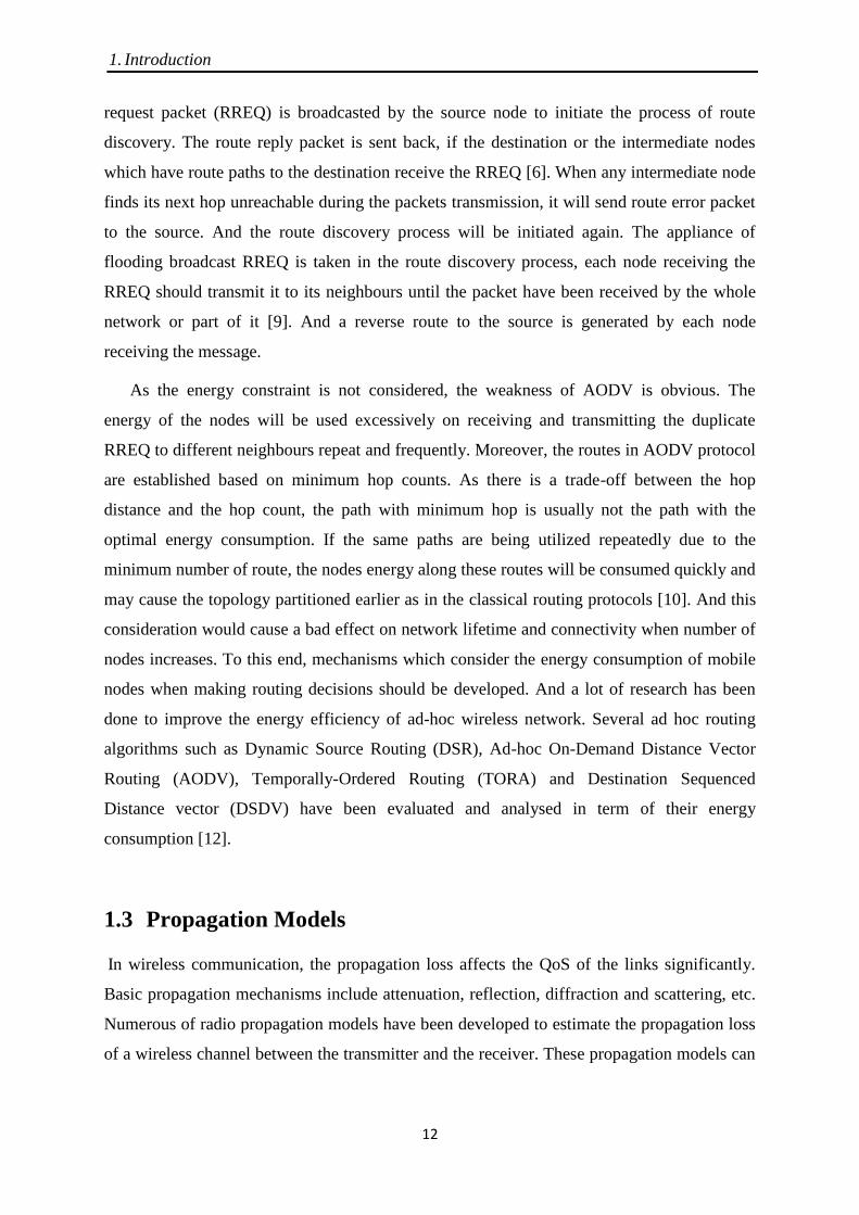
request packet (RREQ) is broadcasted by the source node to initiate the process of route
discovery. The route reply packet is sent back, if the destination or the intermediate nodes
which have route paths to the destination receive the RREQ [6]. When any intermediate node
finds its next hop unreachable during the packets transmission, it will send route error packet
to the source. And the route discovery process will be initiated again. The appliance of
flooding broadcast RREQ is taken in the route discovery process, each node receiving the
RREQ should transmit it to its neighbours until the packet have been received by the whole
network or part of it [9]. And a reverse route to the source is generated by each node
receiving the message.
As the energy constraint is not considered, the weakness of AODV is obvious. The
energy of the nodes will be used excessively on receiving and transmitting the duplicate
RREQ to different neighbours repeat and frequently. Moreover, the routes in AODV protocol
are established based on minimum hop counts. As there is a trade-off between the hop
distance and the hop count, the path with minimum hop is usually not the path with the
optimal energy consumption. If the same paths are being utilized repeatedly due to the
minimum number of route, the nodes energy along these routes will be consumed quickly and
may cause the topology partitioned earlier as in the classical routing protocols [10]. And this
consideration would cause a bad effect on network lifetime and connectivity when number of
nodes increases. To this end, mechanisms which consider the energy consumption of mobile
nodes when making routing decisions should be developed. And a lot of research has been
done to improve the energy efficiency of ad-hoc wireless network. Several ad hoc routing
algorithms such as Dynamic Source Routing (DSR), Ad-hoc On-Demand Distance Vector
Routing (AODV), Temporally-Ordered Routing (TORA) and Destination Sequenced
Distance vector (DSDV) have been evaluated and analysed in term of their energy
consumption [12].
1.3 Propagation Models
In wireless communication, the propagation loss affects the QoS of the links significantly.
Basic propagation mechanisms include attenuation, reflection, diffraction and scattering, etc.
Numerous of radio propagation models have been developed to estimate the propagation loss
of a wireless channel between the transmitter and the receiver. These propagation models can

1. Introduction
13
be divided into two main categories: empirical models and statistic models [13]. Two basic
propagation models are introduced and presented below.
1.3.1 Free Space Propagation Model
Free Space indicates that the propagation path between the transmitter and the receiver is a
clear, unobstructed line-of-sight. The free space propagation loss is caused by the
transmitting signal propagating in every direction all around and the density of power
decreases while the distance increases [14]. The receiving power depending on distance and
influenced by signal wavelength can be found from the Friis free space equation as follows.
where Pt is the transmission power, Pr is the receiving power, Gr and Gt are the antenna gains
at receiver and transmitter respectively, d is the propagation distance, is the radio
wavelength, and Ls is the system loss.
1.3.2 Two-Ray Ground Reflection Model
A single line-of-sight path is rarely the only propagation path between the transmitter and the
receiver in practical cases which makes the results of free space propagation model
inaccurate. Therefore, a model which considers both the direct path and a ground reflection
path is introduced. It is shown [14] that this Two-Ray Ground reflection model provides more
accurate estimation at a long distance than free space model. The received power at distance
d can be predicted according to the equation below.
where ht and hr are the heights of the transmitting and receiving antennas respectively.
1.4 HSDPA Overview
The 3rd
Generation Partnership Project (3GPP) is the forum where standardization is handled
for HSDPA and HSUPA and has been handled from the wideband code division multiple
access (WCDMA) specification release as well [15]. In order to improve the efficiency of the
spectrum utilization, DS-CDMA channel access method multiplexes sub-stream of raw

1. Introduction
14
information bits in WCDMA air interference by modulating the transmitted signals in each
sub-stream utilizing a unique sequence of chips [15]. And each chip has much shorter
duration than the information bit.
Based on the WCDMA air interface, high speed data packet access (HSDPA) is
developed. As this packet-based data service enhances the performance of the WCDMA in
3G communication systems, HSDPA is also known as the 3.5G mobile communication
systems. HSDPA is one of the members in High-Speed Packet Access (HSPA) family.
Current HSDPA deployments support down-link speeds of 1.8, 3.6, 7.2 and 14.0 Megabit/s.
Further speed increases are available with HSPA+, which provides speeds of up to 42 Mbit/s
downlink and 84 Mbit/s with Release 9 of the 3GPP standards [16].
HSDPA introduced a new transport channel—High-Speed Downlink Shared Channel
(HS-DSCH) which is dedicated for high-speed data transmission. Channel-dependent
scheduling is adopted to facilitate air interface channel-sharing between clients. It comprises
three newly introduced physical layer channels: High Speed-Shared Control Channel (HS-
SCCH); the High Speed-Dedicated Physical Control Channel (HS-DPCCH); and the High
Speed- Physical Downlink Shared Channel (HS-PDSCH).
In HSDPA systems, K=5, 10 or 15 spreading codes which use the same QPSK and
MQAM modulation schemes are adopted for one single user to implement multi-channel data
transmission [17]. Adaptive modulation and coding (AMC) technique, which allows the
modulation and coding schemes can be changed according to the signal quality for individual
users, is used to replace the power control functions in WCDMA and can significantly
increase the downlink capacity. Moreover, hybrid automatic repeat-request (HARQ) [17], a
fast physical layer-based retransmission mechanism, is used in HSDPA system to reduce
latency and improve the roundtrip time.
The HSDPA model, which is constructed based on the HSDPA protocol in 3GPP Release
5, is used in the thesis and presented in Chapter 2. In this model, all available physical layer
channels are assumed to be dedicated to one single user. AMC mechanism is implemented to
adjust transmission bit rate for each channel according to the signal quality, which can
explore the optimum solutions on allocating bits and powers in multi-channels.

1. Introduction
15
1.5 Thesis Outline
The following chapters of the thesis are organized as follows. In Chapter 2, the structure of
the HSDPA system is first studied and introduced. Then, the energy utilization problem is
then presented and analysed in HSDPA systems, and related residual energy and achievable
data rate are addressed and tested. In order to solve the problem of the inefficient energy
utilization in HSDPA systems, a two-group resource allocation scheme [18] which assigns
the information bits into two groups of channels with different numbers of bits per symbol
are adopted and analysed carefully. At last, the related work on the MAC DCF study is
reviewed and the MAC DCF service time is studied from analysing and examining a DCF
model which is developed in [19] for multi-hop wireless Ad-Hoc networks. In Chapter 3, the
energy utilization problem for routing scheme in multi-rate networks is addressed. And
energy consumption of each hop along a routing path forms the core part of the cost function.
A trellis-hop diagram approach is presented to find all the possible routing paths of a given
node pair in a network. And a modified Viterbi solution [20] [21] is introduced to reduce the
computational complexity of trellis diagram approach. Moreover, in order to reduce the
computational complexity of discovering the best paths between every two nodes in a
network, a modified Floyd’s algorithm is developed. In Chapter 4, the coded parity packets
approach [22] [23] is studied and analysed. Then based on CPP approach, an adaptable
transmission mechanism is developed to improve the energy efficiency in wireless Ad-Hoc
networks. Finally, the summary of this thesis is provided in Chapter 5, and some future works
are outlined.
2. Two Group Resource Allocation Scheme and MAC DCF service Time
16
Chapter 2
Two Group Resource Allocation Scheme
and MAC DCF Service Time
2.1 Introduction
In this chapter, the HSDPA system used for a single link between two nodes in the
wireless Ad-Hoc Networks is introduced. Moreover, the resource allocation schemes which
can optimum the transmission rate under certain transmission energy are studied and analysed.
Finally, a MAC layer model of wireless Ad-Hoc networks, which is adopted in this project, is
presented.
2.2 High-Speed Downlink Packet Access (HSDPA) System
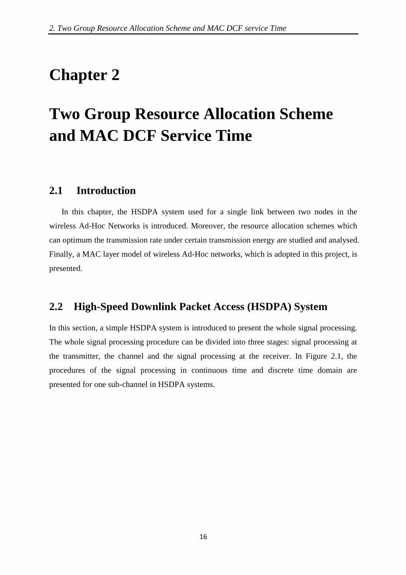
In this section, a simple HSDPA system is introduced to present the whole signal processing.
The whole signal processing procedure can be divided into three stages: signal processing at
the transmitter, the channel and the signal processing at the receiver. In Figure 2.1, the
procedures of the signal processing in continuous time and discrete time domain are
presented for one sub-channel in HSDPA systems.
2. Two Group Resource Allocation Scheme and MAC DCF service Time
17
Figure 2.1 Signal processing and transmission in discrete time and continuous time domains for a single sub-
channel
2.2.1 Signal Processing at the Transmitter
In k-th sub-channel, the coded binary bit stream is passed to the modulation unit and mapped
into symbols bk. then the channel symbol bk is scaled to √ where Ek is the allocation
energy per symbol. After power control procedure, the generated and scaled complex-valued
channel symbol, √ for k-th sub-channel, first separates its real and imaginary
components into two branches, the I (upper) branch and the Q (lower) branch, respectively
[15]. Following on from that, a spreading filter processes on channel symbol components in
both branches. The spreading filter is represented by an N-length vector . A series of N
chips with one chip duration is generated. Then each chip in both branches is
multiplied with a common chip pulse-shaping function to transform the discrete time
signals in chips to continuous time waveforms [15]. The transmitter will then transmit the
continuous time waveform in the radio channel after the waveform has been modulated to the
carrier frequency fc.
2.2.2 Radio Channel
The loss in the radio channel with a certain propagation distance and carrier frequency can be
estimated by various propagation models. For instance, if the channel is non-frequency

2. Two Group Resource Allocation Scheme and MAC DCF service Time
18
selective, the amplitude of the received signal can be expressed as √ , where hk is
the channel gain for k-th sub-channel. At the input of the receiver, received signals are
corrupted by the noise and MAI, and are presented as √ , where
IMAI is the MAI factor and In is the noise [24].
2.2.3 Signal Processing at the Receiver
At the receiver, the received waveform is the convolution of the transmitted waveform
with the channel impulse response h(t) pulsing the additive white noise n(t). Firstly, the
received waveform is demodulated by two demodulation functions with a /2 shift to
baseband signals which separate the real components and imaginary components. Then the
chip-match function is performed to convolve with the signal in both I and Q
branch respectively, and the output is sampled in every Tc seconds. A common filter,
represented by the vector , then operates on the I and Q branches of signals to
despread the channel symbol estimation in every n chips. After the dispreading procedure, the
signal is demapped from symbols to bit streams.
2.3 Rate Allocation in HSDPA Systems
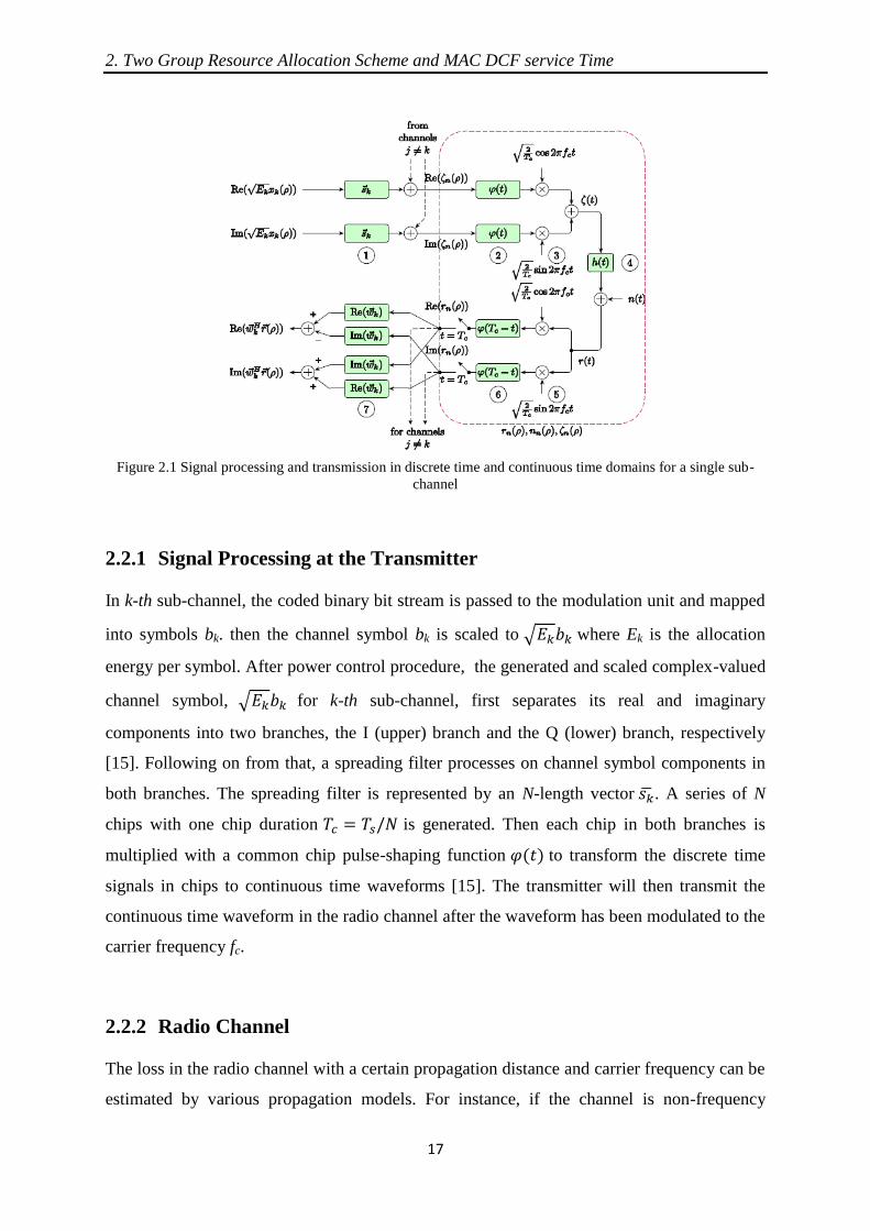
Figure 2.2 illustrates a simplified discrete-time model for HSDPA system with frequency
selective channel, in which the I and Q branches are combined. There are K sub-channels in
this HSDPA system. And the information bits are demultiplexed into K substreams in the
base station. In k-th substream, the information bits are encoded and modulated to complex
symbols, bk, in each Ts seconds. In AMC Units, the amount of information bits in each
symbol for each coded channel is determined. And in Power Units, the channel symbols are
scaled to √ with Ek is the allocated energy per symbol in k-th sub-channel.
Then the symbols are passed through the spreading filters which is different for each
channel to generate a series of N chips per symbol. N is named as the processing gain. Then
the chips of K sub-channels are added together and sent. At the receiver end, the depreading
sequences are adopted to minimize the cross-correlations from the noise and the other coded
channels. Then the information bits in each coded channel are retrieved from the output of the
depreading filters.
2. Two Group Resource Allocation Scheme and MAC DCF service Time
19
Figure 2.2 HSDPA System Structure
2.3.1 Equal Energy and Equal Rate Allocation in HSDPA Systems
Equal energy and equal rate allocation scheme is a method which constraints the powers and
bit rates be to assigned uniformly among all used sub-channels while varying the number of
active sub-channels to achieve the maximum total bit rate.
Consider a wireless link employing multi-code HSDPA with a processing gain of NPG for
K physical layer sub-channel, each channel of which adopts a unique spreading sequence,
hence the K sub-channels are orthogonal to each other. The transmitted data can be
adaptively loaded using AMC at P different rates of
(2.1)
where β represents the incremental amount between any two adjoining bit rate values, which
is named as bit granularity in this thesis. It is defined as for p=1,2,…,P. The
transmitted energy per symbol per channel to achieve the transmission the bit rate bp can be
expressed as
( )
| | p=1, 2… P (2.2)
where h is the amplitude attenuation factor for an interference-free channel, is the gap value
which illustrates the performance difference between the practical modulations and coding

2. Two Group Resource Allocation Scheme and MAC DCF service Time
20
schemes with the optimal cases, and is the noise samples variance at the output of the
chip-match filter.
In order to accomplish the equal rate allocation in K active sub-channels, the total
available energy is allocated to K parallel channels equally. As it is assumed that the channels
are non-frequency selective, the SNR are the same at the input of K channels. As the sum of
the energy transmitted in K parallel channels to provide bit rate bp in each channel, cannot
exceed the given transmission energy ET. We have . And related SNR for each
channel satisfies
, where SNRT and SNR(bp) can be found from
| |
(2.3)
( ) | |
(2.4)
According to the equations above, the bit rate per symbol per channel bp can be expressed
as follows.
( )
(2.5)
(2.6)
Therefore, the equal rate and power method can achieve the maximum total bit rate as
follow.
(2.7)
where K is the number of active parallel channels which can be chosen from 1 to 15.
2.3.2 Residual Energy Utilization
In the previous section, the equal energy allocation is introduced. However, this approach
results in a considerable amount of residual energy which is not adopted to transmit any
useful information. This residual energy is defined as below.
( ) ( ( ) ( )) (2.8)
where e(bp) is the incremental energy. The incremental energy to realize an additional data
rate of β bits per symbol from a lower data rate of bp to bp+1 is defined as
2. Two Group Resource Allocation Scheme and MAC DCF service Time
21
( ) ( ) ( )
| | (2.9)
According to equation (2.8) and (2.9), when the equal rate allocation scheme is adopted in
multi-code HSDPA systems, an inefficient usage of the limited available energy, which
usually results in reducing the total data rate in HSDPA system, is raised.
2.3.3 Two-group Resource Allocation Scheme
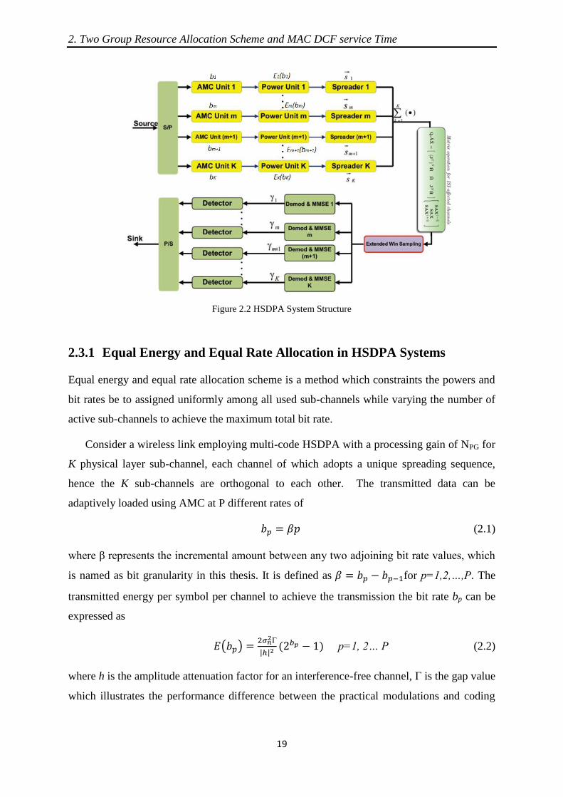
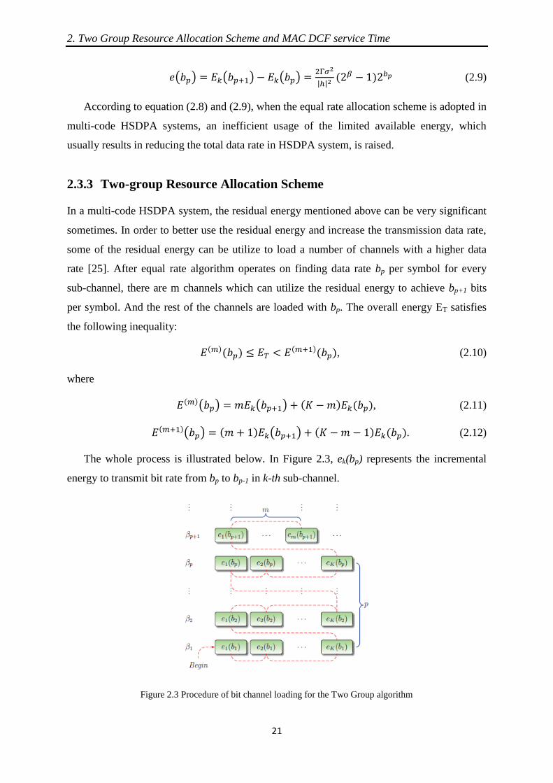
In a multi-code HSDPA system, the residual energy mentioned above can be very significant
sometimes. In order to better use the residual energy and increase the transmission data rate,
some of the residual energy can be utilize to load a number of channels with a higher data
rate [25]. After equal rate algorithm operates on finding data rate bp per symbol for every
sub-channel, there are m channels which can utilize the residual energy to achieve bp+1 bits
per symbol. And the rest of the channels are loaded with bp. The overall energy ET satisfies
the following inequality:
, (2.10)
where
( ) ( ) , (2.11)
( ) ( ) . (2.12)
The whole process is illustrated below. In Figure 2.3, ek(bp) represents the incremental
energy to transmit bit rate from bp to bp-1 in k-th sub-channel.
Figure 2.3 Procedure of bit channel loading for the Two Group algorithm

2. Two Group Resource Allocation Scheme and MAC DCF service Time
22
The maximums overall bit rate is acquired as:
(2.13)
which indicates the overall data rate is maximized when the bit rate bp is allocated to K-m
channels, and the bit rate bp+1 is allocated to m channels. This joint allocation of bit rates and
transmission energy is named as two-group resource allocation scheme, in which the
channels loading bit rate bp are low-rate channels, while the channels loading bp+1 are called
high-rate channels [25].
Under the same assumptions made above and By knowing a given set of parameters
which include h, , , β and ET, as well as a set of discrete bit rate values , the bit
rate index p for the low-rate channels can be derived as
(⌊
| |
⌋ ) (2.14)
After obtain the value of p, the number of high-rate channels which loading with bit rate
bp+1 can then be determined as
⌊
( ) ⌋ (2.15)
After the lower data rate index p is derived from equation (2.14) and the number of higher
data rate channel m is computed from equation (2.15), the transmission process can operate
by transmitting bp bits per symbol in K-m sub-channels while transmitting bp+1 bits per
symbol in the other m channels.
2.3.4 Resource Allocation in Frequency Selective Channels
When the multi-code HSDPA system operates over an environment with multipath
propagation feature and the wireless link is rather frequency selective than flat, the signature
sequences in parallel channels become non-orthogonal at the receiver end, and channels are
interfered by signals in the other channels and in other symbol periods. For the channels with
interference, two-group resource allocation scheme can implemented to achieve the
maximum overall transmission bit rate as well.
2. Two Group Resource Allocation Scheme and MAC DCF service Time
23
Consider a HSDPA system with frequency selective channels, the data is passed through
the serial to parallel encoder first in which information are separate into K blocks. The
orthogonal signature sequences are given by
. (2.16)
A discrete time channel impulse vector is used for the frequency selective channel with L
propagation paths.
(2.17)
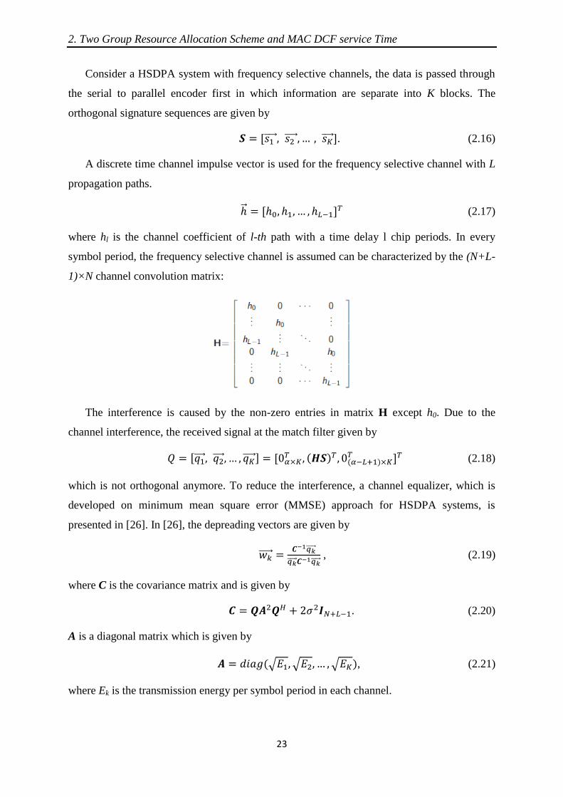
where hl is the channel coefficient of l-th path with a time delay l chip periods. In every
symbol period, the frequency selective channel is assumed can be characterized by the (N+L-
1)×N channel convolution matrix:
The interference is caused by the non-zero entries in matrix H except h0. Due to the
channel interference, the received signal at the match filter given by
(2.18)
which is not orthogonal anymore. To reduce the interference, a channel equalizer, which is
developed on minimum mean square error (MMSE) approach for HSDPA systems, is
presented in [26]. In [26], the depreading vectors are given by
, (2.19)
where C is the covariance matrix and is given by
. (2.20)
A is a diagonal matrix which is given by
√ √ √ , (2.21)
where Ek is the transmission energy per symbol period in each channel.

2. Two Group Resource Allocation Scheme and MAC DCF service Time
24
In this case the output SNRs are calculated as follows:
(2.22)
where k is the index of the parallel channel from 1 to K.
When Inter-symbol Interference is considered, a window extended model presented in [27]
is adopted to improve the system performance and total capacity. By extending the window
length by α-chip on each side, this window records a part of the next symbol period and a
portion of the previous symbol period. The new receiver signature sequence matrix is then
given by
(2.23)
where
(2.24)
And
. (2.25)
On the other hand, the correspond covariance matrix is modified as
, (2.26)
where ⊗ √ √ √ .
The whole process of the two-group resource allocation schemes can be divided into two
parts such as Equal rate allocation and Residual energy allocation.
Algorithm 1. Equal rate allocation algorithm (finding bp)
1: Set j=1, and initialize
and initialize the amplitude diagonal
matrix
⊗ √ √ √
2: Set i=1, yk=bj, and for k=1,2...K
3: Compute the covariance matrix at this stage:

2. Two Group Resource Allocation Scheme and MAC DCF service Time
25
4: Renew the energy
( )
5: Update the amplitude diagonal matrix:
⊗ √ √ √
6: Set i=i+1
7: If for k=1,...,K and i Imax (for example Imax=50) go back to step 3.
Otherwise go to the next step.
8: Set j=j+1, and go to step 2, when j<P and
∑ ,. Otherwise for k=1,…, K and p=j-1. is the
allocated energy to achieve the transmission data rate bp in k-th channel.
After the energy of transmitting the data rate bp bits per symbol is allocated for each channel,
the residual energy is given by ∑ . The residual energy is utilized
to transmit bp+1 bits per symbol in m channels.
Algorithm 2. Residual energy allocation algorithm (finding m)
1: Sort the channels in ascending order, for example the first channel corresponds to the
channel ( ) ( ) .
2: Set j=1 and calculate the amplitude diagonal matrix
⊗ √ √ √
3: Set i=1, for k=1,…,j, for k=j+1,…,K, and
for k=1,2...K.
4: Compute the covariance matrix at this stage:
4: Update the energy
( )
5: Update the amplitude diagonal matrix:
⊗ √ √ √
6: Set i=i+1
7: If for k=1,...,K and i Imax (for example Imax=50) go back to step 4.
Otherwise go to the next step.
2. Two Group Resource Allocation Scheme and MAC DCF service Time
26
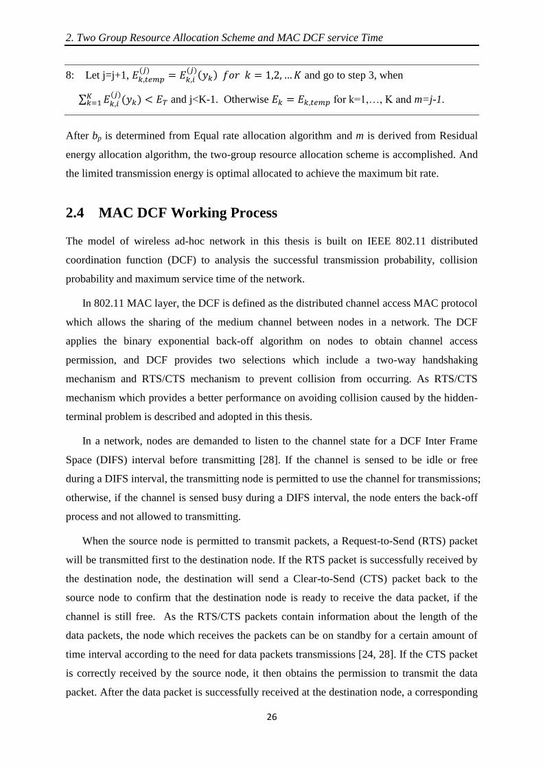
8: Let j=j+1,
and go to step 3, when
∑
and j<K-1. Otherwise for k=1,…, K and m=j-1.
After bp is determined from Equal rate allocation algorithm and m is derived from Residual
energy allocation algorithm, the two-group resource allocation scheme is accomplished. And
the limited transmission energy is optimal allocated to achieve the maximum bit rate.
2.4 MAC DCF Working Process
The model of wireless ad-hoc network in this thesis is built on IEEE 802.11 distributed
coordination function (DCF) to analysis the successful transmission probability, collision
probability and maximum service time of the network.
In 802.11 MAC layer, the DCF is defined as the distributed channel access MAC protocol
which allows the sharing of the medium channel between nodes in a network. The DCF
applies the binary exponential back-off algorithm on nodes to obtain channel access
permission, and DCF provides two selections which include a two-way handshaking
mechanism and RTS/CTS mechanism to prevent collision from occurring. As RTS/CTS
mechanism which provides a better performance on avoiding collision caused by the hidden-
terminal problem is described and adopted in this thesis.
In a network, nodes are demanded to listen to the channel state for a DCF Inter Frame
Space (DIFS) interval before transmitting [28]. If the channel is sensed to be idle or free
during a DIFS interval, the transmitting node is permitted to use the channel for transmissions;
otherwise, if the channel is sensed busy during a DIFS interval, the node enters the back-off
process and not allowed to transmitting.
When the source node is permitted to transmit packets, a Request-to-Send (RTS) packet
will be transmitted first to the destination node. If the RTS packet is successfully received by
the destination node, the destination will send a Clear-to-Send (CTS) packet back to the
source node to confirm that the destination node is ready to receive the data packet, if the
channel is still free. As the RTS/CTS packets contain information about the length of the
data packets, the node which receives the packets can be on standby for a certain amount of
time interval according to the need for data packets transmissions [24, 28]. If the CTS packet
is correctly received by the source node, it then obtains the permission to transmit the data
packet. After the data packet is successfully received at the destination node, a corresponding

2. Two Group Resource Allocation Scheme and MAC DCF service Time
27
acknowledgement (ACK) packet will be sent from the destination node to the source node to
confirm the reception of the data packet. The Short Inter-Frame Space (SIFS) is used to
separate the transmission of all packets which include RTS, CTS, DATA and ACK. SIFSs
provide the time for transition between transmitting and receiving of source node and
destination node. Figure 2.4 illustrates the process of distributed coordination function.
Figure 2.4 DCF Transmission
The time consumed for one full successful transmission, which is defined as the sum of
the time consumed for every control packet transmission, data packet transmission and the
time intervals, is given by [19]
(2.27)
where E{P}=L/rdata is the time consumed for data packet transmission with a packet length L-
bit and bit rate rdata. and are the time slots for control packets
transmission. These control packets are transmitted at a certain rate in DCF. In this thesis, this
rate is chosen as 1 Mb/s. is the time interval among the packets transmissions. is the
propagation delay which is very small.
On the other hand, the time consumed for detecting a collision occurrence is provided
below.
(2.28)
It means that if the destination node does not receive the RTS packet in a time duration tc, a
collision is considered to happen. The detailed parameter values of IEEE 802.11 are provided
in Table 1.

2. Two Group Resource Allocation Scheme and MAC DCF service Time
28
2.5 MAC DCF Service Time
Marcelo M. Carvalho developed a scalable DCF model [19] for the analytical study of
medium access protocol operating in multi-hop wireless Ad-Hoc networks. This model is
built by expressing each layer’s functionality in probabilistic terms. In the PHY layer, the
probability of a successful frame reception is concerned. And in MAC layer, the model is
concerned with its scheduling rate.
2.5.1 Successful Frame Reception Probability
Let V represent the finite set of |V|=n nodes which construct the network in this section, and
let denote the subset of the nodes whose power can be received at node r below the
threshold. When |Vr|=nr and the frame is transmitted by node i, there are combinations
of active transmitting nodes in subset Vr. And let represent the set of these
combinations.
Provided the considerations above, the probability that a frame, which is transmitted by
node i, is received at node r successfully can be expressed as follows:
∑
∑ |
= ∑
(2.29)
The above formalism allows for the consideration of any radio channel model and PHY-
layer aspect for computation of the probability of successful frame reception
conditioned on a certain MAI level [19]. And the scheduling probability (transmission
2. Two Group Resource Allocation Scheme and MAC DCF service Time
29
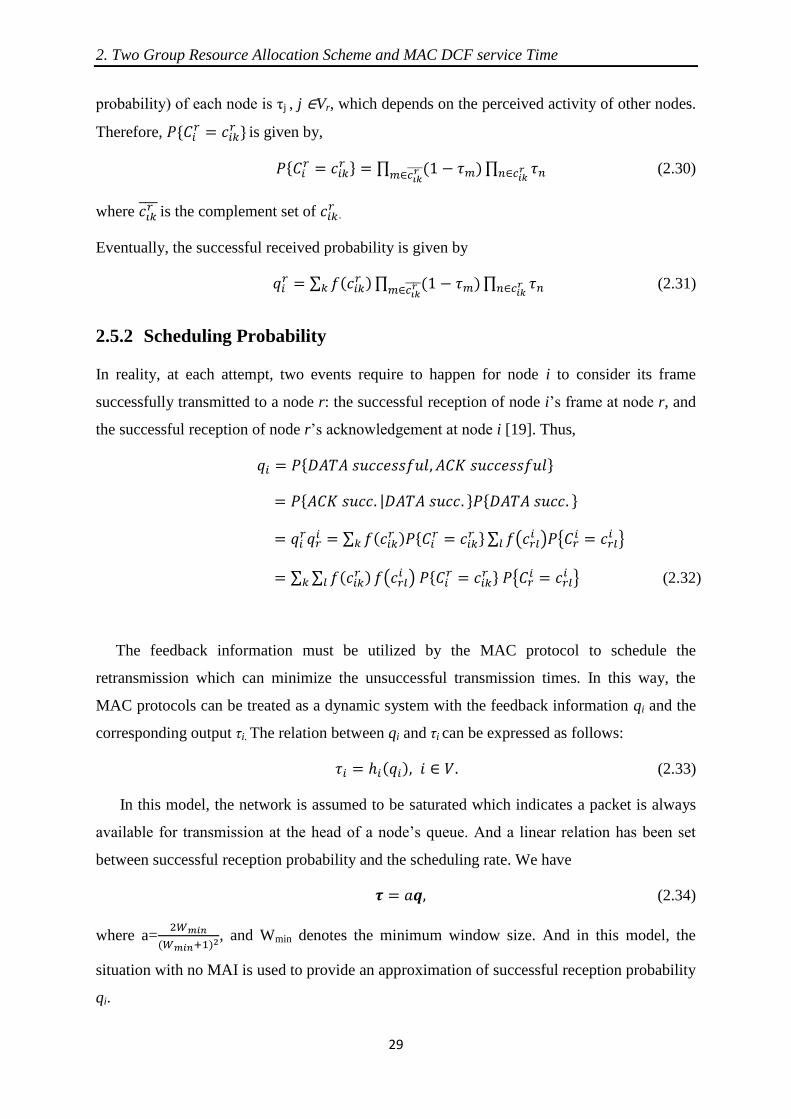
probability) of each node is τj , j ∈Vr, which depends on the perceived activity of other nodes.
Therefore,
is given by,
∏ ∈ ∏ ∈
(2.30)
where
is the complement set of
.
Eventually, the successful received probability is given by
∑
∏ ∈ ∏ ∈
(2.31)
2.5.2 Scheduling Probability
In reality, at each attempt, two events require to happen for node i to consider its frame
successfully transmitted to a node r: the successful reception of node i’s frame at node r, and
the successful reception of node r’s acknowledgement at node i [19]. Thus,
|
∑
∑ (
) {
}
∑ ∑ (
)
{
} (2.32)
The feedback information must be utilized by the MAC protocol to schedule the
retransmission which can minimize the unsuccessful transmission times. In this way, the
MAC protocols can be treated as a dynamic system with the feedback information qi and the
corresponding output τi. The relation between qi and τi can be expressed as follows:
∈ (2.33)
In this model, the network is assumed to be saturated which indicates a packet is always
available for transmission at the head of a node’s queue. And a linear relation has been set
between successful reception probability and the scheduling rate. We have
(2.34)
where a=
, and Wmin denotes the minimum window size. And in this model, the
situation with no MAI is used to provide an approximation of successful reception probability
qi.

2. Two Group Resource Allocation Scheme and MAC DCF service Time
30
( )
∏ ( τ ) ∈ ∏ τ ∈
( )
∏ ( ) ∈ ∏ ∈
( )
∑ ∈ (2.35)
By making ( )
, and considering the set V with all nodes in the network
topology, we have
∑ ∈ (2.35)
∑ ∈ (2.36)
∑ ∈ (2.37)
where ri denotes the intended receiver of node i. The equations above can be expressed in
matrix form.
(2.38)
where
∈
(2.39)
Therefore, the successful transmission probability qi can be derived from
(2.40)
The probability of successful frame reception conditioned on a certain MAI level can be
found from
(2.41)
where L is the frame length, denotes the SINR at node r for bits transmitted by node i
when none of node r’s interferers transmits., and is the bit error rate for a certain SINR
level .
2. Two Group Resource Allocation Scheme and MAC DCF service Time
31
2.5.3 Modelling the IEEE 802.11 DCF
In the backoff algorithm of IEEE 802.11 DCF, the states of channel can be classified in terms
of three mutually exclusive events: Ec={collision}, Ei={idle channel}, and Es={successful
transmission}. To compute the channel state probabilities, the work by Bianchi [29] is
utilized.
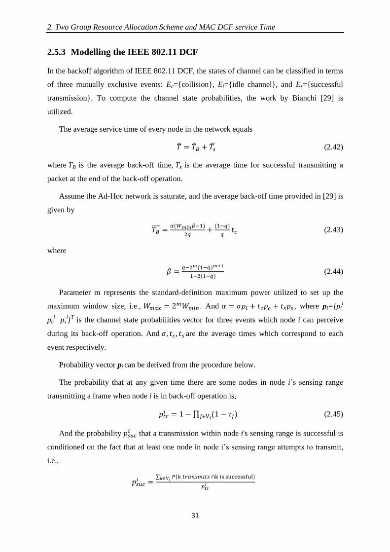
The average service time of every node in the network equals
(2.42)
where is the average back-off time, is the average time for successful transmitting a
packet at the end of the back-off operation.
Assume the Ad-Hoc network is saturate, and the average back-off time provided in [29] is
given by
(2.43)
where
(2.44)
Parameter m represents the standard-definition maximum power utilized to set up the
maximum window size, i.e., . And , where pi=[pii
pci ps
i]
T is the channel state probabilities vector for three events which node i can perceive
during its back-off operation. And are the average times which correspond to each
event respectively.
Probability vector pi can be derived from the procedure below.
The probability that at any given time there are some nodes in node i’s sensing range
transmitting a frame when node i is in back-off operation is,
∏ ∈
(2.45)
And the probability that a transmission within node i's sensing range is successful is
conditioned on the fact that at least one node in node i’s sensing range attempts to transmit,
i.e.,
∑ ∈

2. Two Group Resource Allocation Scheme and MAC DCF service Time
32
∑ | ∈
∑ ∈
(2.46)
Therefore, the probability of a successful transmission occurs within node i’s sensing
range, psi is then ps
i = ptr
ipsuc
i. And the probability of idle channel within node i’s sensing
range is then pii = 1-ptr
i, and the probability pc
i which a collision happens within node i’s
sensing range is given by
[30]. After this channel state probabilities
vector is determined, the average backoff time can be identified from equation (2.43) and the
average service time can be derived from equation (2.42).
2.6 Simulation and Performance Evaluation
In this section, the simulations focus on the performance of the wireless Ad-Hoc networks
with HSDPA system implemented on every wireless link. The first simulation is done to test
and analyse the theoretical maximum achievable data rates of the one-group loading scheme
and the two-group resource allocation scheme.
In Figure 2.5, a number of different transmission mechanisms are tested along with the
two-group resource allocation scheme to inspect the theoretical overall achievable data rate in
bits per symbol for a range of the received SNR, SNRT. In this simulation, several parameter
values are given as ∈ , β=2 and . The general rate allocation method is
provided as
{
( ) ( )
The single-code CDMA has only one channel to transmit data bit, and the required SNR
for the single-code CDMA is , where bp is the achievable data rate per
symbol. The data rate per symbol achieved by this scheme is much lower than the data rates
of the other two schemes.
The equal energy loading scheme and two-group resource allocation scheme are tested in
HSDPA system with K=15 sub-channels. According to equation (2.5) (2.6), the data rate of
one-group loading scheme is computed and plotted in Figure 2.5. It is clear that the data rate
of this scheme is much higher than the achievable data rate of the single-code CDMA scheme.

2. Two Group Resource Allocation Scheme and MAC DCF service Time
33
The achievable data rate of the two-group resource allocation scheme is plotted as red line in
Figure 2.5. As observed in this figure, the total data rate of the two-group resource allocation
scheme is the highest in these three transmission mechanisms. It is because the residual
transmission energy, which introduced in section 2.3.2, is well utilized by two-group resource
allocation scheme. It should be noted that the reason for the total achievable data rates of one-
group loading scheme and the two-group resource allocation scheme are equal to each other
at last is the maximum bp is b3=6. When the SNR is very large, the maximum achievable data
rate of two-group resource allocation scheme is limited to bits per
symbol. It means 15 sub-channels are fully loaded with the same bits per symbol
which is equal to the single-group loading scheme.
Figure 2.5 The data rate realized by different resource allocation schemes
However, in reality, the propagation distances in communication systems are relatively
long which always leads to multipaths and frequency selective channels. Therefore, the
second simulation is run to take the multipath effects into consideration. Consider two nodes
in a wireless Ad-Hoc network, the maximum transmission range is 200 meters. The one-
group loading scheme and the two-group resource allocation scheme are simulated with
different propagation distance from 10 meters to 200 meters between two nodes. In this
simulation model, the values of the parameters are set as ∈ , β=2 and .
And a spreading matrix with number of sub-channels, K=15 and processing gain, NPG=16 are
0 5 10 15 20 25 30 35 40 450
20
40
60
80
100
120
140
160
180
Two-group loading with 15 HSDPA coded channels
Single-goup loading with 15 HSDPA coded channels
Single-code CDMA

2. Two Group Resource Allocation Scheme and MAC DCF service Time
34
generated. The propagation loss is derived by using the two-ray ground reflection
propagation model from equation (1.2). According to [13], the chiprate is set to 3.84Mbits/s,
the transmission power at the source node is adjusted to 10 mW, and the power of noise is
. And the additive white Gaussian noise of variance is given as
(2.47)
where represents the chip period. The overall available energy can be derived from
(2.48)
And the resultant total received signal-to-noise ratio is
(2.49)
where h denotes the propagation loss in dB.
The results are plotted in Figure 2.6 and 2.7.
Figure 2.6 System capacity and bit rate achieved by One-group HSDPA system and Two-group HSDPA system
as a function of distance
From Figure 2.6, it is observed that when the distance increases, the total achievable data
rates of both one-group loading scheme and two-group resource allocation scheme decrease.
It is because the propagation loss increases when the distance increases which leads to a
reduction in the received signal power and the received SNR. And according to Figure 2.6,
two-group resource allocation scheme has a larger total data rate than one-group loading
scheme when the propagation distance exceeds 40 meters. And when the propagation
0 20 40 60 80 100 120 140 160 180 2000
0.5
1
1.5
2
2.5x 10
7
Distance (m)
Bit R
ate
(bps)
Two-group HSDPA
Energy Rate HSDPA (one group)

2. Two Group Resource Allocation Scheme and MAC DCF service Time
35
distance is larger than around 170 meters, the one-group loading scheme cannot support data
transmission while the two-group resource allocation scheme still can achieve a total bit rate
around 2 Mbits/s. It is because the one-group loading scheme can only use K=5, 10, 15
channels for transmission, however the two-group resource allocation scheme adopts a
channel adaptive HSDPA system. The bit rates in Figure 2.6 are plotted along the received
SNR in Figure 2.7. It is clear that due to its better residual energy utilization, the two-group
resource allocation scheme has a larger bit rate than one-group loading scheme at certain
SNR.
Figure 2.7 System capacity and bit rate achieved by One-group HSDPA system and Two-group HSDPA system
as a function of SNR
Based on the DCF service time presented in this chapter, the final simulation has run to
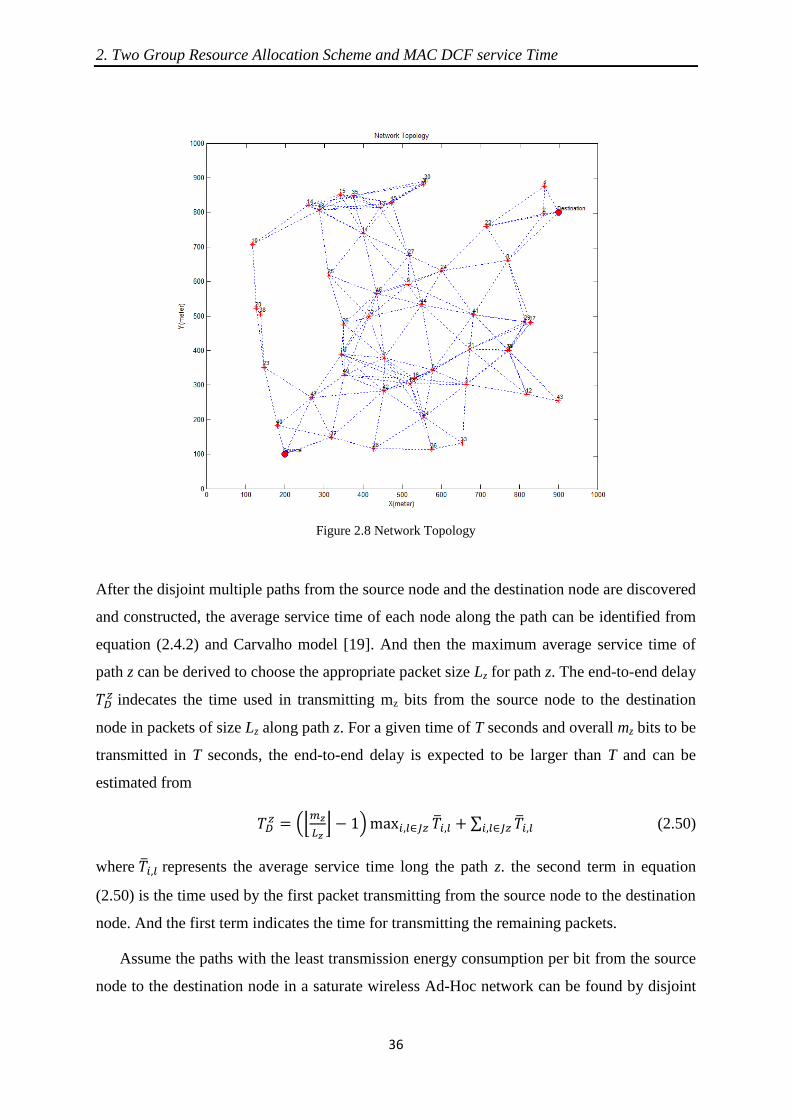
estimate and measure the end-to-end delay in a wireless Ad-Hoc networks. In Figure 2.8, a
wireless Ad-Hoc network with 50 randomly distributed nodes is presented on an x-ygrid. And
nodes in this networ are assumed stable with their ID marked besides them. The maximum
transmission range of each node is set at 200 meter which indicates the signal can be detected
at the received within this range. The maxmimum carrier sensing range at the MAC layer,
which is defined as the range that the transmission power can be perceived, is given as 400
meters. And the nodes which can communicate with each other are linked with blue dash
lines in Figure 2.8.
0 10 20 30 40 50 600
0.5
1
1.5
2
2.5x 10
7
SNR in dB
Bit R
ate
(bps)
Two-group HSDPA
Equal Energy HSDPA (one group)
2. Two Group Resource Allocation Scheme and MAC DCF service Time
36
Figure 2.8 Network Topology
After the disjoint multiple paths from the source node and the destination node are discovered
and constructed, the average service time of each node along the path can be identified from
equation (2.4.2) and Carvalho model [19]. And then the maximum average service time of
path z can be derived to choose the appropriate packet size Lz for path z. The end-to-end delay
indecates the time used in transmitting mz bits from the source node to the destination
node in packets of size Lz along path z. For a given time of T seconds and overall mz bits to be
transmitted in T seconds, the end-to-end delay is expected to be larger than T and can be
estimated from
(⌊
⌋ ) ∈ ∑ ∈ (2.50)
where represents the average service time long the path z. the second term in equation
(2.50) is the time used by the first packet transmitting from the source node to the destination
node. And the first term indicates the time for transmitting the remaining packets.
Assume the paths with the least transmission energy consumption per bit from the source
node to the destination node in a saturate wireless Ad-Hoc network can be found by disjoint

2. Two Group Resource Allocation Scheme and MAC DCF service Time
37
multipath routing discovery schemes. The disjoint multiple paths are shown in Firgure 2.9.
The indexes of the nodes along two paths are given as
The best path: 1→40→47→49→19→26→32→46→9→24→22→2→50
The second best path: 1→37→42→18→16→5→21→41→8→50
Both one-group loading scheme and two-group rresource allocation scheme are implemented
to assign achieveable data rate for each path.
Figure 2.9 Network Topology with Disjoint Multiple Routing Paths
After the total data bit mz for each path is allocated, the appropriate packet size is determined
as
∈ (2.51)
And the number of packet can be derived from
⌊
⌋ (2.52)
As sometimes there are some remaining bits in mz after Nz times of packet transmission, the
packet size is then updated as
⌈
⌉ (2.53)
0 100 200 300 400 500 600 700 800 900 10000
100
200
300
400
500
600
700
800
900
1000
2
3
4
5
67
8
9
1011
12
131415
16
17
18
19
20
21
22
23
2425
26
27
28
29
3031
32
33
34
35
3637
38
39
40
41
4243
44
45
46
47
48
49
Source
Destination
2. Two Group Resource Allocation Scheme and MAC DCF service Time
38
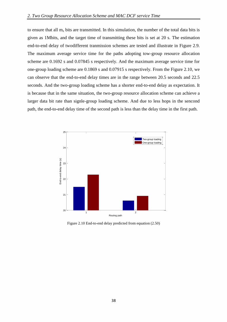
to ensure that all mz bits are transmitted. In this simulation, the number of the total data bits is
given as 1Mbits, and the target time of transmitting these bits is set at 20 s. The estimation
end-to-end delay of twodifferent tranmission schemes are tested and illustrate in Figure 2.9.
The maximum average service time for the paths adopting tow-group resource allocation
scheme are 0.1692 s and 0.07845 s respectively. And the maximum average service time for
one-group loading scheme are 0.1869 s and 0.07915 s respectively. From the Figure 2.10, we
can observe that the end-to-end delay times are in the range between 20.5 seconds and 22.5
seconds. And the two-group loading scheme has a shorter end-to-end delay as expectation. It
is because that in the same situation, the two-group resource allocation scheme can achieve a
larger data bit rate than signle-group loading scheme. And due to less hops in the sencond
path, the end-to-end delay time of the second path is less than the delay time in the first path.
Figure 2.10 End-to-end delay predicted from equation (2.50)
1 220
21
22
23
24
25
Routing path
End-t
o-e
nd d
ela
y t
ime (
s)
Two-group loading
One-group loading
3. Disjoint Multipath Routing Discovery Schemes
39
Chapter 3
Disjoint Multipath Routing Discovery
Schemes
3.1 Introduction
Unlike the traditional cellular communication systems in which the communications between
the mobile nodes and administration infrastructure are direct without relays, the wireless Ad-
Hoc networks do not have a centralized point for administration. The transmission and
receiving between the source and the destination are realized by forwarding information from
one node to another through a routing path. And the relay nodes consume some extra energy.
Moreover, each node in these networks operates on constrained battery power, which
eventually gets exhausted with time, thus energy is one of the most important constraints to
be considered. To transmit more information in a certain lifetime, the routing path discovery
schemes which consider the energy constraint should be developed.
3.2 Minimization of Energy Consumption Per Bit
A saturated wireless Ad-Hoc network is considered in this project with N randomly
distributed nodes on a two-dimension grid. The maximum achievable data rate between each
wireless link depends on the propagation distance between the transmitter and the receiver
which causes a different amount of SNR for data transmission. For this reason, different
wireless routes may have various numbers of bits per symbol to transmission. And different
packet sizes are adjusted and adopted in different routing paths according to the computed
energy consumption per bit for the path.
Consider a source node and destination node in a network, a total number of M bits to be
transmitted over Z routing paths linking from the source to the destination in T seconds. The
total transmission data rate between the source and the destination is provided as
(3.1)

3. Disjoint Multipath Routing Discovery Schemes
40
Regarding path z, mz bits of information are transmitted over this path at a rate of bits
per second for a given T seconds, where the total number of bits M is the sum of the bits
transmitted in all the routing path exist which is defined as ∑ . And
is the
service time, which is defined and identified in Chapter 3, between node i and node j. Node i
and node j are the adjacent nodes along the routing path. Lz is the packet size in bit
transmitted over path z. Based on the parameters given above, the maximum transmission
data rate over path z is given by
∈
(3.2)
where Jz represents the set of nodes in path z. And the total transmission data rate can be
expressed as
∑
∑
∈
(3.3)
The amount of energy consumed to transmit mz bits at a data rate of mz/T bits per second
over path z is given by
∑
∈
∑
∈
(3.4)
which requires an equivalent MAC power of and amount of energy consumed
per bit over path z is
∑
∈ (3.5)
Thus, when the energy consumption for every routing path is known, the total consumed
energy is proposed to be minimized as
∑ (3.6)
In order to minimize the total energy ET, the least consumed amounts of energy per bit,
Eb,z must be determined as equation above. To achieve the load balancing, the amount of
energy which are allocated to each path are equal, such as . Once all possible
routing paths without shared nodes are discovered by using the least amount of energy per bit
Eb,z as the path metrics, the number of bits which should be assigned to each path can be
3. Disjoint Multipath Routing Discovery Schemes
41
derived. Given the total number of bits M to be transmitted, the expression of the energy
consumed at each path is then given as follows.
∑ ∑
(3.7)
∑
(3.8)
Equation (3.8) can be substituted in equation (3.4) to acquire the number of bits per path, and
mz is given by
∑
(3.9)
Therefore, the minimum energy consumed for transmitting mz bits over path z is determined.
The routing path discovery schemes which consider energy constraint and use Eb,z as the path
metrics are presented in the following section.
3.3 The Trellis-hop Diagram Routing Discovery Scheme
Consider a wireless Ad-Hoc network with N nodes and a trellis-hop diagram can be adopted
to determine all the possible routing paths. The diagram is organized by arranging N×N
nodes in which the first arranging the N nodes are in a column and similar columns of nodes
are repeatedly drawn up to N-1 times next to the first column. According to the links between
nodes in the network topology, the routing paths are determined by drawing the links from
the source node to its neighbouring nodes, which are denoted in the next column [21]. And
the same process starts from the drawing the link to the adjacent neighbouring node to the
destination node.
A simple example which shows the whole procedure of Trellis-hop Diagram Routing
Discovery approach in a 5-node network is presented below. The topology of the network is
illustrated in Figure 3.1, and the distance between every two nodes is labelled beside each
link in red.

3. Disjoint Multipath Routing Discovery Schemes
42
Figure 3.1 A 5-node Network Topology
From Figure 3.2-3.4, it is clear that two paths pass through neighbouring node 2 of the
source node, two paths pass through source node’s neighbouring node 3 and two paths pass
through neighbouring node 4. Therefore, there are overall six paths from the source to the
destination being determined by trellis-hop diagram. Then the energy consumed per bit for
each path can be derived according to equation (3.5), and the one with the least energy
consumption will be identified as the best path.
However, it is obvious that this approach has a significant extensive computational
complexity. For the N-node Ad-Hoc network, this approach needs to compute (N-1)! times to
find the path with the least cost, which is not efficient.
Figure 3.2 The First Neighbour of Source Node for Trellis-hop Diagram

3. Disjoint Multipath Routing Discovery Schemes
43
Figure 3.3 The Second Neighbour of Source Node for Trellis-hop Diagram
Figure 3.4 The Third Neighbour of Source Node for Trellis-hop Diagram
3.4 Modified Viterbi Algorithm
An improved version of Trellis-hop diagram approach which is named modified Viterbi
algorithm is developed in [21] to improve the computational efficiency of Trellis-hop
diagram approach. Instead of finding all the possible routes, this modified Viterbi algorithm
groups the link-joint routing paths shared the same relay nodes and selects the routing path
with the lowest cost as the best paths. The other high-cost paths are removed from the routing
table during the routing path discovery process. Before commencing the routing path

3. Disjoint Multipath Routing Discovery Schemes
44
discovery, the adjacency matrix is generated. The adjacency matrix for the topology in Figure
3.1 is given as
[
]
The entry of one in the adjacency matrix indicates the two nodes, which are represented
by the indices or the row and column numbers of the entry, can communicate with each other.
After the adjacent matrix is constructed, the data rate matrix can be formed as below.
000
0
000
00
00
4,52,5
5,43,42,41,4
4,31,3
5,24,21,2
4,13,12,1
rr
rrrr
rr
rrr
rrr
The difference between the data rate matrix and the adjacency matrix is that the entries
which are equal to one in the adjacency matrix are replaced with the data rate between the
corresponding adjacent nodes. As the transmission power allocated in all the nodes are equal,
the data rate matrix is symmetric, where . It means the data rates are equal in both
directions of any two adjacent nodes. Once the propagation path loss is derived by using the
propagation model mentioned in equation (1.2), the received energy can be determined. Then
the two-group resource allocation scheme is adopted to maximize the transmission data rate
between every two nodes. Finally, the modified Viterbi algorithm can perform on the rate
matrix to find the optimum paths.
In modified Viterbi algorithm, besides updating the total path link cost for all the latest
paths which are discovered at each hop, it investigates the next nodes which are adjacent to
the current nodes as well. In this process, the next node of each path cannot be the node
which is already included in this path before. And all the incomplete paths are recorded in the
incomplete routing table. Once the next node of the routing path is the destination node, this
routing path is set to a completed path and stored in the completed routing table. If there are
more than one incomplete routing paths which pass through the same next node, the routing
path with the largest data rate and least energy consumption will be selected for further
investigation, while the other paths will be abandoned. These processes will be iterated until
all the nodes are investigated in and the optimal routing paths are found. There are three main

3. Disjoint Multipath Routing Discovery Schemes
45
routing path tables for this algorithm and these are: (1) the completed routing path table, (2)
the incomplete routing path table, and (3) the abandoned routing path table.
Figure 3.5-3.8 illustrate how this proposed algorithm operates at each hop level. For
simplification and easier understanding, the abandoned routing path table shown in each
figure only contents the abandoned paths at each step. Firstly, the neighbouring nodes of the
source node are reached in one hop. A group of uncompleted routing paths are generated in
this step, ie. {1, 2},{1, 3} and {1, 4}. In the next step, the nodes within two-hop distance
from the source node are searched. The link costs are calculated using equation (3.4), and the
routing paths, which share the same destination nodes in this hop, with the least cost will be
remained for next step process, while the other routing path will be abandoned. In this step,
the discarded paths are represented by dash lines. And routing path {1, 2, 5} is stored in the
completed routing table. Figure 3.8 shows the process of the forth step. In each step, the
algorithm ensures the paths which have the least energy cost with the same destination node
in this hop are remained, and the next nodes chosen for each current incomplete routing path
are not included by this path before. After the algorithm is finished, the abandoned routing
path table and the incomplete routing path table are clear. As shown in Figure. 3.8, the final
completed routing paths based on current topology are {1, 2, 5}, and {1, 2, 3, 4, 5}. And one
of these three paths, which has the least energy consumption, will be selected as the best path.
Figure 3.5 The First Hop Level for Routing Paths Discovery

3. Disjoint Multipath Routing Discovery Schemes
46
Figure 3.6 The Second Hop Level for Routing Paths Discovery
Figure 3.7 The Third Hop Level for Routing Paths Discovery
Figure 3.8 The Forth Hop Level for Routing Paths Discovery
3. Disjoint Multipath Routing Discovery Schemes
47
It is obvious that as many incomplete paths with large link costs are not consider for
further routing discovery in modified Viterbi algorithm, the modified Viterbi algorithm has a
much better computational efficiency than trellis-hop diagram approach. The modified
Viterbi algorithm can reduce the computational complexity down to O(N) for a N-node
networks, when the maximum number of neighbouring nodes is much lower than N [31].
In order to find all the disjoint lowest cost routing paths, the paths with the lowest cost is
first found and all the nodes along this path are removed from the network topology. Then the
routing discovery scheme is re-invoked to find the second lowest cost path in the new
network topology which is constructed by the rest of the nodes. This process iterates until all
the disjoint routing paths are discovered.
3.5 Modified Floyd Algorithm
The modified Viterbi algorithm proposed in previous section is efficient to find the best path
for one-pair node (one source and one destination) with a computational complexity of O(N).
However, if this algorithm is adopted to find the shortest paths in a multi-source and multi-
destination scenario, the computational complexity of finding all the vertex pairs will
increase to O(N3) in a N-node network. To further investigate and enhance the routing paths
discovery algorithm, a modified Floyd algorithm is developed to minimize the computational
complexity of finding the shortest paths for all-pair nodes in a wireless ad hoc network.
In Floyd’s algorithm, a distance matrix is generated and utilized to discover the shortest
paths between all-pair of nodes in a network [32]. Its main operation theory is concluded as
follow. A distance weigh matrix D(0)
is first constructed in which the each element denotes
the distance between two adjacent nodes. Then the one-hop distances between each pair of
nodes are computed and compared with the corresponding elements in distance matrix D(0)
.
The smaller distances for each pair of nodes are updated and stored in matrix D(1)
. This
process operates iteratively, and the distance matrixes for various hops are derived as D(2)
,
D(3), …, D
(k-1), D
(k). The whole operation stops until D
(k)=D
(k-1) which means the elements in
distance matrix cannot be reduced anymore. And the least distances between all-pair of nodes
are stored in D(k)
which becomes the shortest distance matrix. The Floyd’s algorithm is
summarized as follows.
Step 1: Initial distance matrix D(0)
=(dij(0)
),

3. Disjoint Multipath Routing Discovery Schemes
48
where
{
weight of edge
Step 2: Generate iterative distance matrix D(k)
=(dij(k)
), where
{
| .
Step 3: If D(k+1)
=D(k)
, loop stops; otherwise repeat step 2.
According to [32], the time complexity of Floyd’s algorithm is O(N3) which is very high
and not efficient for large networks. To improve the computational complexity of both the
Floyd’s algorithm and data rate allocation along the routing paths, a modified Floyd’s
algorithm is developed in the thesis.
As same as the Modified Viterbi Algorithm presented previously, in order to maximize
the data rate of the routing path under certain transmission energy, the two-group resource
allocation scheme is applied to derive the maximum data rate between every pair of the
adjacent nodes. In this process, the equation (1.2) is used to derive the propagation loss which
affects the SNR and the received energy in every wireless link. From equation (2.2) (2.3)
(2.10) (2.15), it is clear that the only external factor effects the data rate distribution is the
distance between two nodes. When the distance (d) increases, the propagation loss increases
proportionately to the quartic power of distance (d4). And the received energy decreases when
the propagation loss increases, which leads to a reduction in transmission data rate.
Therefore, , in order to reduce the computational complexity, the quartic power of the
distance between each two nodes ( ) which are in each other’s transmission range is
adopted as the metric of a weigh matrix, instead of utilizing the maximum data rate between
every pair of the adjacent nodes to construct a rate matrix in modified Viterbi algorithm. For
instance, the weigh matrix of the topology in Figure 3.1 is given by
0
0
0
0
0
4,52,5
5,43,42,41,4
4,31,3
5,24,21,2
4,13,12,1
ww
wwww
ww
www
www

3. Disjoint Multipath Routing Discovery Schemes
49
0
0
0
0
0
4
4,5
4
2,5
4
5,4
4
3,4
4
2,4
4
1,4
4
4,3
4
1,3
4
5,2
4
4,2
4
1,2
4
4,1
4
3,1
4
2,1
dd
dddd
dd
ddd
ddd
.
The shortest path in this algorithm is the path has the least sum of the quartic power of all the
hop distances along the routing path, which is defined as ∑
∈ .And JZ is the set
of the nodes along the path.
After analyzing the basic Floyd’s algorithm, four points are investigated in and modified
to accelerate the calculation speed and reduce the computational complexity.
1) It is not difficult to find that when deriving the elements wij(k)
of the weigh matrix W(k)
,
the elements wst(k)
(s=1,2,3…i-1; t=1,2,…n) in previous i-1 rows, and the previous j-1
elements wit(k)
(t=1,2,3…j-1) in ith
row have already been calculated. In this way, the Gauss
Seidel algorithm [34] can be applied in these elements to derive the shortest path. As
wij(k)
=min{wir(k-1)
+wrj(k-1)
|r=1,2,…,n}, when r<j, we have wir(k)≤ wir
(k-1); when r<i, we have
wrj(k)
≤wrj(k-1)
. Thus it is possible to use wir(k)
and wrj(k)
to replace wir(k-1)
and wrj(k-1)
. And the
shortest path equation can be written as
wij(k)
= min{min{wir,r<j(k)
+wrj,r<i(k)
}, min{wir,r<j(k)
+wrj,r>j(k-1)
}, min{wir,r>j(k-1)
+wrj,r<i(k)
},
min{wir,r>j(k-1)
+wrj,r>i(k-1)
}}. (3.10)
2) In the Floyd’s algorithm, backtrace is adopted to find the shortest path from the
source to the destination. It means that in order to find the shortest path between node i and
node j, the algorithm have to trace back to the previous steps to determine how wij(k)
comes
from. For example, let wij(k)
= wir(k-1)
+ wrj(k-1)
. Then, the algorithm will check how wir(k-1)
and
wrj(k-1)
are determined. This process iterates until the elements in W(0)
are reached. To
simplify this complicated approach, a routing matrix which records all the routing paths for
different pairs of nodes is generated as L(k)
=(lij(k)
). For example, let lij(k)
={ lir(k-1)
, node r, lrj(k-
1)}, the elements in lij
(k) denote the nodes which the path from node i to node j passes through.
When the iteration ends and the routing matrix becomes to L(k)
, the shortest path between
node i and node j can be expressed as i lij(k)
j.
3) As in wireless Ad-Hoc network, the distance from node i to node j is equal to the
distance from node j to node i, we have dij4=dji
4 and wij
(k)=wji
(k). In this way, if wij
(k) has
already been determined, it is not necessary to use more iterations to derive wji(k)
.
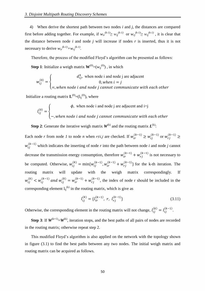
3. Disjoint Multipath Routing Discovery Schemes
50
4) When derive the shortest path between two nodes i and j, the distances are compared
first before adding together. For example, if wir(k-1)
≥ wij(k-1)
or wrj(k-1)
≥ wij(k-1)
, it is clear that
the distance between node i and node j will increase if nodes r is inserted, thus it is not
necessary to derive wir(k-1)
+wrj(k-1)
.
Therefore, the process of the modified Floyd’s algorithm can be presented as follows:
Step 1: Initialize a weigh matrix W(0)
=(wij(0)
) , in which
{
when node i and node j are adjacent
Initialize a routing matrix L(0)
=(lij(0)
), where
{
when node i and node j are adjacent and i=j
Step 2: Generate the iterative weigh matrix W(k)
and the routing matrix L(k)
:
Each node r from node 1 to node n when r≠i,j are checked. If
or
which indicates the inserting of node r into the path between node i and node j cannot
decrease the transmission energy consumption, therefore
is not necessary to
be computed. Otherwise,
for the k-th iteration. The
routing matrix will update with the weigh matrix correspondingly. If
, the index of node r should be included in the
corresponding element lij(k)
in the routing matrix, which is give as
(3.11)
Otherwise, the corresponding element in the routing matrix will not change,
.
Step 3: If W(k+1)
=W(k)
, iteration stops, and the best paths of all pairs of nodes are recorded
in the routing matrix; otherwise repeat step 2.
This modified Floyd’s algorithm is also applied on the network with the topology shown
in figure (3.1) to find the best paths between any two nodes. The initial weigh matrix and
routing matrix can be acquired as follows.

3. Disjoint Multipath Routing Discovery Schemes
51
0
0
0
0
0
4
4,5
4
2,5
4
5,4
4
3,4
4
2,4
4
1,4
4
4,3
4
1,3
4
5,2
4
4,2
4
1,2
4
4,1
4
3,1
4
2,1
dd
dddd
dd
ddd
ddd
.
08.907.4565
8.9001.2519.29108.2308
1.25100.1062
7.45659.291005.7
8.23080.10625.70
According to step 2, as
, it is not necessary to calculate
. We have
and
correspondingly.
: as none of the elements in the first row of W(0)
is smaller than
(except
), it is
not necessary to calculate
. We have
, and in the routing matrix
.
: as there is an element in the first row of W(0)
which is smaller than
,
is defined
as
=
=1062.0. The corresponding element in routing
matrix remains the same,
. And
,
.
: as there are two elements in the first row of W(0)
are smaller than
,
is defined
as
{
}
, which means node
3 is inserted into the path between node 1 and node 4. And
. Moreover,
,
.
Similarly, the other elements in W(1)
and L(1)
can be determined.

3. Disjoint Multipath Routing Discovery Schemes
52
{
}
,
.
,
=
,
.
,
.
{
}
,
.
,
.
{
}
,
{
} {
} .
,
.
{
}
,
{
} .
,
.
,
.
,
.
,
.
{
}
,
{
} .
,
.
,
.
,
.
,
.
After the derivation above, we have

3. Disjoint Multipath Routing Discovery Schemes
53
08.909.3414.14116.2399
8.9001.2516.13201.1313
9.3411.25105.10690.1062
4.14116.13205.106905.7
6.23991.13130.10625.70
44,3,14,3
3,13
41
4,3,13,11
4,33
As W(1)
≠ W(0)
, the iteration should be carried out until W(k)
≠ W(k-1)
. W(2)
and L(2)
are
obtained as follows.
08.909.3414.14116.2399
8.9001.2516.13201.1313
9.3411.25105.10690.1062
4.14116.13205.106905.7
6.23991.13130.10625.70
44,3,14,3
3,13
41
4,3,13,11
4,33
It is clear that W(2)
= W(1)
, and the algorithm terminates. Therefore, the best paths of every
two nodes in the network are recorded in the routing matrix. For example, according to the
routing matrix, the best path between node 1 and node 5 passes through node 3 and node 4.
After the best path is found between the source node and the destination node, two-group
resource allocation scheme will then adopted to determine the maximum data rate for each
single hop along the best path. Obviously, instead of determining the data rate between every
two nodes in the network, this algorithm reduces the computational complexity greatly. In
Figure 3.9, the modified Viterbi algorithm and modified Floyd’s algorithm are adopted to
find the disjoint multiple routing paths.

3. Disjoint Multipath Routing Discovery Schemes
54
Figure 3.9 Disjoint Multiple Routing Discoveries
3.6 Performance Evaluation
As mention in section 3.4, the computational complexity for trellis-hop diagram routing
method is O(N3). And the modified Viterbi algorithm can enhance the efficiency significantly
and reduce the computational complexity to O(N). On the other hand, the computational
complexity of the modified Viterbi algorithm in finding the all-pair best paths is O(N3). In
order to order to efficiently find the best paths between every two nodes in a network, the
modified Floyd’s algorithm is developed to enhance the efficiency of the traditional Floyd’s
algorithm. Compared with the traditional Floyd’s algorithm, the number of iterations is
reduced in the modified algorithm. As the comparisons of
(
)
are done before deriving
,
is
not necessary to be calculated at each iteration. Thus, the computational complexity is less
than O(N3). Moreover, after the analysis, it is not difficult to find that at k-iteration to
0 100 200 300 400 500 600 700 800 900 10000
100
200
300
400
500
600
700
800
900
1000
2
3
4
5
67
8
9
1011
12
131415
16
17
18
19
20
21
22
23
2425
26
27
28
29
3031
32
33
34
35
3637
38
39
40
41
4243
44
45
46
47
48
49
Source
Destination
0 100 200 300 400 500 600 700 800 900 10000
100
200
300
400
500
600
700
800
900
1000
2
3
4
5
67
8
9
1011
12
131415
16
17
18
19
20
21
22
23
2425
26
27
28
29
3031
32
33
34
35
3637
38
39
40
41
4243
44
45
46
47
48
49
Source
Destination
0 100 200 300 400 500 600 700 800 900 10000
100
200
300
400
500
600
700
800
900
1000
2
3
4
5
67
8
9
1011
12
131415
16
17
18
19
20
21
22
23
2425
26
27
28
29
3031
32
33
34
35
3637
38
39
40
41
4243
44
45
46
47
48
49
Source
Destination

3. Disjoint Multipath Routing Discovery Schemes
55
derive
, the nodes with
, which cannot communicate with the node i, will
not be considered. Therefore, it just needs to consider mi nodes which can communicate with
node i. Let mi be the number of edges connected with node i. As there are N2 elements in the
weigh matrix, it needs mi times operation to derive and the computational complexity at
k-iteration is ∑
. And
is equal to
in this case, when
is derived,
is known as well. Therefore, the computational complexity of this modified Floyd’s
algorithm is
which is less than the computational complexity of the traditional
Floyd’s algorithm.

4. Coded Parity Packet Scheme
56
Chapter 4
Coded Parity Packet Scheme
4.1 Introduction
In telecommunication systems, retransmissions are carried out to achieve the reliable packet
transmission when data packets fail to be detected at the receiver end. In wireless Ad-Hoc
networks, unnecessary repetitive retransmissions cause not only an increase in the end-to-end
delay, but also a rise in the energy consumption of nodes, which would reduce the network
lifetime significantly when the nodes are battery powered. Increasing the transmission energy
per symbol can increase the output SNR and reduce the number of retransmissions. However,
as this approach consumes a great amount of additional energy, the network lifetime would be
significant reduced. Therefore, the packet error rate should be minimized by lowering the
increase in the required energy close to the theoretical minimum value [35]. It is essential to
develop a channel coding scheme to reduce the gap value in wireless Ad-Hoc networks,
which keeps the packet error rate low and decreases the number of retransmissions whilst
providing lower energy consumption. Hence, the Coded Parity Packet Approach [22] is
developed by M. K. Gurcan to lower the packet error rate and then reduce the retransmission
times and the required energy. Coded Parity Packet Approach includes an outer and inner
coding scheme to provide alternative additional information value for the decoding process.
Without changing the effective code rate, the outer coding technique adjusts the number of
source and parity packets, from which the additional input information values are produced on
the receiver end to be alternatively fed into the decoding process to recover the received
packets.
4.2 System Overview
It is considered that the system is constructed by three main blocks, such as the transmitter,
the channel and the receiver, as shown in Figure 4.1. The discrete information from the data

4. Coded Parity Packet Scheme
57
source is in binary form. The data sequences are generated in blocks of K symbols, and each
block is denoted as a (K × 1)-dimensional vector , in which each of its element is
represented as uk ∈ {±1}, for k = 1,2,...,K.
The source data block is segmented into V equal-sized source packets, and each of them
represented as an ((N-Np) ×1) - dimensional vector, , where N-Np=K/V. And then the outer
coder will use these source packets to produce E-V parity packets in addition to the V source
packets which are denoted as . After this, Np cyclic redundancy check (CRC) bits are
appended to each parity packets which yields (N×1) – dimensional vector . At last, these
packets are inner coded to create (B×1)-dimensional vector for e=1, 2…, E. before
transmission in wireless channel, a modulated symbol vector is produced from every coded
packet by adopting an M-QAM scheme. The generated symbols are transmitted over a
noise-corrupted channel, in which the white Gaussian noise vector is denoted by with a
variance of .
At the receiver end, after the noise-corrupted symbols are demodulated, the
required (B × 1)-dimensional soft channel output vector ( ), which is the input of the
iterative soft decoding process, is derived from the received symbol vector [23]. Then, the
CRC-appended packets is estimated by the soft-in-hard-out decoding process at the
receiver. The CRC algorithm is re-invoked to check the integrity of these estimates [36]. Each
CRC-checked vector is represented as . Before the final estimates are de-segmented, if any
of the first V parity packets , , …, , which are the source packets … , fail then a
hard decoding mechanism will operate to recover these packets.
Figure 4.1 The Coded Parity Packets Approach Model
4.3 Channel Encoder
The channel encoder can be separated to twp parts – outer encoder and inner encoder.

4. Coded Parity Packet Scheme
58
4.3.1 The Outer Encoder
The data block after packets segmentation can be represented in a matrix as U = [ , , …,
]. These source packets are passed through the outer encoder to produce E packets, S =
[ ,…, ]. There are E-V parity packets in these E packets. The formula to generate these E
packets can be expressed as below.
⊗ (4.1)
As there are E-V parity packets, LE=2E-V-1
subsets of associated packets are generated. If
the outer code rate is fixed at
, the number of the subsets, LE can be controlled by
adjusting the integer numbers V0 and E0 of the source and parity packets to V = V0 × α and E
= E0 × α such that the outer code rate
remains unchanged, where α is the
adjustment parameter [23].
Table above shows that the number of distinct subsets of the parity packets, LE, is
controllable, therefore it can be increased to enhance both the soft and hard decoding process
on the receiver end.
The matrix G in equation (4.1) can be generated from
(4.2)
where IV is a (V×V)-dimensional identity matrix which is used to regenerate the V source
packets. And PJ(sel)
is the generator for E-V parity packets. P is a (V×Z)-dimensional matrix,
while J(sel)
is a (Z×(E-V))-dimensional parity selector matrix. Each column in matrix P can be
derived by
(4.3)

4. Coded Parity Packet Scheme
59
where bin(D) represents a (V×1)-dimensional binary vector which corresponds to a number D.
D can be treat as the index which points from 3 to 2V-1 so long as D is not a power of two. JV
is a (V×V)-dimensional matrix which has its cross diagonal elements equal to 1 and other
elements equal to 0.
To ensure that the parity selector matrix, J(sel)
,selects E source and parity packets from
which 2E-V-1
subsets of parity packets are available to generate 2E-V-1
subsets, every source
packet must be a neighbour of at least one of the parity packets [23]. The simplest way to
make every source packet as a neighbour of at least one parity packet is making this parity
packet be generated from the last column in matrix P, because =[1,1,1,…,1]T. The
remaining E-V-1 parity packets can be produced by using the remaining columns in P. Thus,
PJ(sel)
in equation (4.2) can be written as
(4.4)
where . Therefore, J(sel)
can be
written as follows
(4.5)
According to the J(sel)
generated above, the parity packets can be derived from equation
(4.1) and (4.2).
4.3.2 The Inner Encoder
The inner encoders are the standard Turbo encoders with an inner code rate of rin= N/B. The
CRC-appended parity packets, produced by the outer encoder are sent to the inner
encoders. Then a M-QAM modulation scheme operates on these coded parity packets. A
modulated packet, is Gray-mapped from a Turbo-coded parity
packet which is represented as a (B×1)-dimensional vector
. And
the vectors in can be expressed as . As Turbo codes are
adopted as the inner codes, which are generated from the parity packets, there are three
categories of the coded parity bits. The first category is the systematic bit,
; the
4. Coded Parity Packet Scheme
60
second category is the first parity bit,
; the third category is the second parity bit,
These three types of bits depend on the puncturing performed on the Turbo codes for
n=1,…,N, np1=1,…,Np1, np2=1,…, Np2, where N + Np1 + Np2 = B.
4.4 Channel Decoder
In this section, the decoding process of Coded Parity Packet approach is described.
The received packet is given by , and the corresponding
channel soft output, as the source of input soft information for soft decoding, is defined as
which is given by
( )
∈
|| || ∈
|| || . (4.6)
Unlike [37] which makes an assumption that the channel gain is unity, and
are two
sets of symbols which denote the sets of symbols in which the mi-th component of (m×1)-
vector, , ie. , equal to 0 and 1 respectively. Hence, the members in set and
are represented by and respectively.
At the receiver side, E standard Turbo decoders are working in parallel, and each of them
has two component decoders. The channel soft outputs of each packet are demultiplexed into
two sequences. The first sequence which includes the LLRs of the systematic bits,
and the first set of parity bits,
for = 1, . . . , and = 1, . . . , is fed into the
first component decoder. And the second sequence, which comprises the LLRs of the
systematic bits,
and the second set of parity bits,
, is fed into the second
component decoder. The LLRs for the parity bits are produced according to the Turbo code
rate adopted, rin= N/B. The channel soft outputs provided from the systematic bits,
,
are defined as the apriori LLRs.
(
) (
) ( )
( ), (4.7)
(
) (
) ( )
( ). (4.8)
where (
) and (
) represent the apriori LLRs of the first component
decoder and second component decoder respectively. The extrinsic LLR, , and the
external extrinsic LLR,
, which are generated from the previous iteration, are zero in the
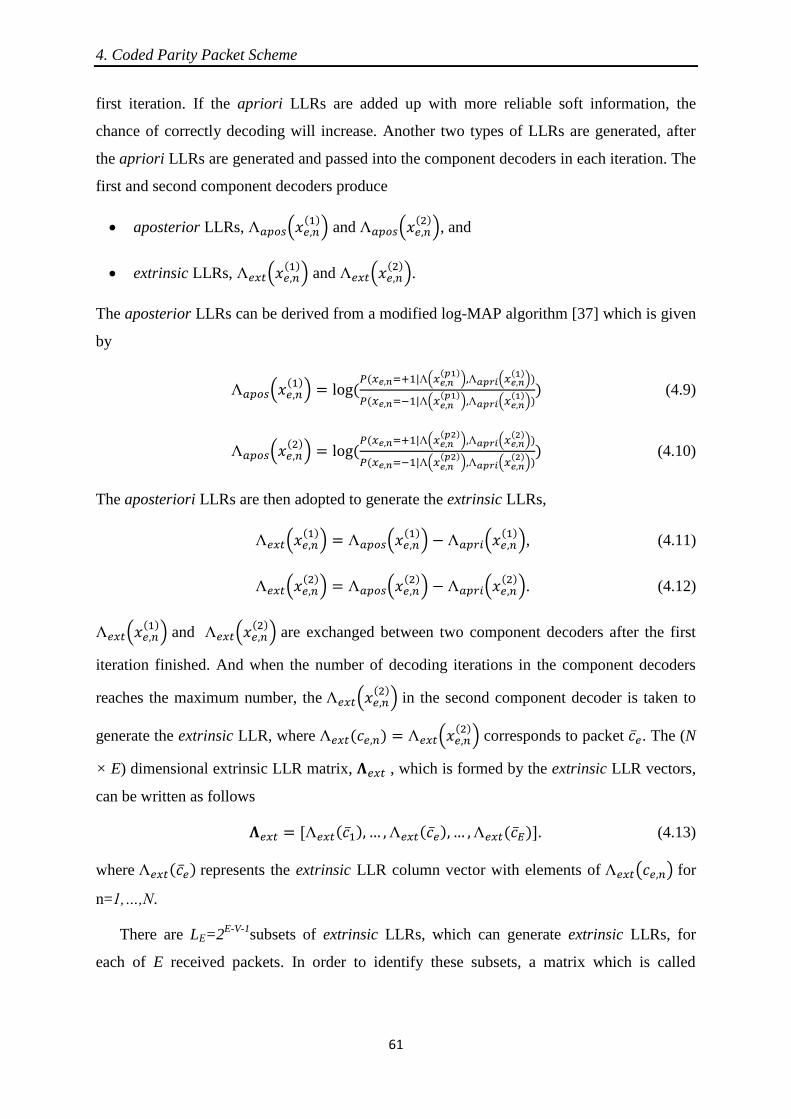
4. Coded Parity Packet Scheme
61
first iteration. If the apriori LLRs are added up with more reliable soft information, the
chance of correctly decoding will increase. Another two types of LLRs are generated, after
the apriori LLRs are generated and passed into the component decoders in each iteration. The
first and second component decoders produce
aposterior LLRs, (
) and (
), and
extrinsic LLRs, (
) and (
).
The aposterior LLRs can be derived from a modified log-MAP algorithm [37] which is given
by
(
) | (
) (
)
| (
) (
) (4.9)
(
) | (
) (
)
| (
) (
) (4.10)
The aposteriori LLRs are then adopted to generate the extrinsic LLRs,
(
) (
) (
), (4.11)
(
) (
) (
). (4.12)
(
) and (
) are exchanged between two component decoders after the first
iteration finished. And when the number of decoding iterations in the component decoders
reaches the maximum number, the (
) in the second component decoder is taken to
generate the extrinsic LLR, where (
) corresponds to packet . The (N
× E) dimensional extrinsic LLR matrix, , which is formed by the extrinsic LLR vectors,
can be written as follows
. (4.13)
where represents the extrinsic LLR column vector with elements of ( ) for
n=1,…,N.
There are LE=2E-V-1
subsets of extrinsic LLRs, which can generate extrinsic LLRs, for
each of E received packets. In order to identify these subsets, a matrix which is called
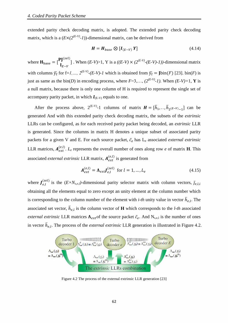
4. Coded Parity Packet Scheme
62
extended parity check decoding matrix, is adopted. The extended parity check decoding
matrix, which is a (E (2(E-V)
-1))-dimensional matrix, can be derived from
⊗ (4.14)
where
. When (E-V)>1, Y is a ((E-V) (2
(E-V)-(E-V)-1))-dimensional matrix
with columns for f=1,…, 2(E-V)
-(E-V)-1 which is obtained from [23]. bin(F) is
just as same as the bin(D) in encoding process, where F=3,…, (2(E-V)
-1). When (E-V)=1, Y is
a null matrix, because there is only one column of H is required to represent the single set of
accompany parity packet, in which I(E-V) equals to one.
After the process above, 2(E-V)
-1 columns of matrix can be
generated And with this extended parity check decoding matrix, the subsets of the extrinsic
LLRs can be configured, as for each received parity packet being decoded, an extrinsic LLR
is generated. Since the columns in matrix H denotes a unique subset of associated parity
packets for a given V and E. For each source packet, has Le associated external extrinsic
LLR matrices,
. Le represents the overall number of ones along row e of matrix H. This
associated external extrinsic LLR matrix,
is generated from
for (4.15)
where
is the (E×Ns,e,l)-dimensional parity selector matrix with column vectors,
obtaining all the elements equal to zero except an unity element at the column number which
is corresponding to the column number of the element with i-th unity value in vector . The
associated set vector, is the column vector of H which corresponds to the l-th associated
external extrinsic LLR matrices of the source packet . And Ns,e,l is the number of ones
in vector . The process of the external extrinsic LLR generation is illustrated in Figure 4.2.
Figure 4.2 The process of the external extrinsic LLR generation [23]
4. Coded Parity Packet Scheme
63
According to the definition presented above, the associated external extrinsic LLR matrix,
can be expressed as
. (4.16)
The simplified extrinsic LLRs combination function mentioned in [38] is given by
|
|∏
, (4.17)
where and
represent the elements of external extrinsic LLR vector and
the extrinsic LLR vector respectively for n=1,…,N. this simplified calculation is iterate for
n=1,…,N to acquire the LLR vector which is then obtained as the external extrinsic
LLR vector at the l-th iteration,
. Therefore, at any single external
iteration, only a single external extrinsic LLR vector is produced. The external iteration will
terminate once the maximum iteration number is reached or the packet is successfully
decoded. After obtaining ,
, (
) and (
), the apriori LLRs,
which are derived from the equation (4.7) (4.8), are enhanced to continue the decoding
process.
If the received packets are not successfully decoded in the iterative soft decoding process
which presented above, a packet-based hard decoding approach is adopted to solve this
problem. After all the successfully decoded packets are hard decided from the soft bits
provided by the iterative soft decoding process and denoted as for e=1,…,E, the integrity
of these packets are checked by the CRC algorithm. And are used to represents the output
packets. To successfully hard decode a received packet, the equation below should be
satisfied.
for (4.18)
where is introduced in the iterative soft decoding process, and is a (E×E)-dimensional
diagonal matrix which is defined as
, (4.19)
The diagonal components are the elements, of vector , are all zero except for those
with the indices equal to the indices of the successfully decoded packet. For example when
E=5, indicates that the first, the forth and the fifth received packets are soft
decoded successfully.

4. Coded Parity Packet Scheme
64
If the equation (4.18) is satisfied, the e-th packet can be recovered as follows.
(4.20)
where is a (E×N)-dimensional matrix in which the rows are produced after the iterative
soft decoding process, .
Obviously, the performance of the hard decoding process is enhanced as more selections
for bit-wise XOR combinations between packets are available to recover the failed packets.
Therefore, when α increases and increases, the packet error rate will be
reduced.
4.5 Performance Analysis of CPP Approach in Wireless Ad-Hoc
Networks
In this section, transmission scheme and re-transmission schemes are first explained and
analysed for the point-to-point transmission. Then an adjustable transmission protocol for
wireless Ad-Hoc network is developed and presented.
Consider the wireless transmission on a single hop between two nodes in a wireless Ad-
Hoc network. It is assumed that the location of each node is stable. The transmission energy
can be written as , where n denotes the number of bits, and Eb represents the energy
required to transmit one single bit. Eb is influenced by the distance between two nodes and
the resource allocation scheme.
The packet error rate, , measures the probability of a packet is detected error at the
receiver. This probability mainly depends on the network protocols and the packet size. And
many uncontrollable and unpredictable factors can influence it as well. The bit error rate,
is assumed to be independent on different bits. And the data packet error rate without re-
transmission for a packet with k bits is given by
(4.21)
A re-transmission is usually requested to reduce the packet error rate when the data
packet is detected erroneous at the receiver. It is assumed the errors in the received packets
can be detected at the receiver end. The packet error rate after α times re-transmission can be
reduced to

4. Coded Parity Packet Scheme
65
(4.22)
It is clear that when the bit error rate is fixed at a certain value, the packet error rate
increases when the packet size increases. However, some other bits are contented in every
packet besides the information bits, such as the packet header. Therefore, though the packet
error rate can be reduced by adopting a smaller packet size, a larger overhead in term of
transmission energy and bandwidth is raised due to less information data in each packet.
Detained studies on the trade-off between the packet size and the overhead are analysed in
[39].
4.5.1 Basic Retransmission Schemes
Three re-transmission schemes in wireless communication systems are considered and
presented below. For notational convenience, several mathematical notations are presented
here. Let k bits in one packet. denotes the bit error rate. represents the packet error rate
without re-transmission. And Eb is the energy per bit.
Case I: Time Sensitive Re-transmission
If errors are detected in the received packet, a re-transmission request will be sent from
the receiver node to the transmitter node. In this time sensitive retransmission mechanism, if
the packet is incorrect as before after one re-transmission, no more re-transmission request
will be sent. And this packet will be abandoned and treated as a loss packet. And the expected
transmission energy and the packet loss probability are provided as
= (1 - (1- )k)2
= (4.23)
(4.24)
where denotes the expected transmission energy, and is the packet loss probability.
Case II: Certain Packet Loss Rate Re-transmission
In this scheme, the packet loss rate is required to be less than or equal to a certain value.
And the packet will be retransmitted until the requirement is satisfied. This mechanism can
be used to guarantee the service quality.
Number of retransmission: α = (4.25)
Expected transmission energy: =
, (4.26)

4. Coded Parity Packet Scheme
66
where α is the number of re-transmission, and β denotes the packet loss rate threshold.
Case III: Content Sensitive Re-transmission
In this mechanism, the re-transmission will be requested until the packet is correctly
received. Some situations with a high requirement on the accurate data utilize this mechanism.
It is an extreme situation of the second case when the threshold of the packet loss rate, β
→0 and the number of retransmission α →∞. The expected
Expected transmission energy:
. (4.27)
4.5.2 Transmission with CPP Approach
According to the analysis on Coded Parity Packet presented in the previous section, it is clear
that the CPP approach can reduce the packet error rate significantly. By using the associated
parity packets, the packet error rate for a set of V source packets and E-V parity packets can
be reduced to
, (4.28)
where is the packet error rate for only one subset of associated parity packet is used in
iterative soft decoding process [23]. And is introduce in section 5.3. On the
other hand, the CPP approach reduces the packet error rate while increases the transmission
energy on transmitting extra parity packets and redundant bits in Turbo coding which is not a
small amount of energy. Therefore, CPP approach can greatly enhance the performance of
the network and reduce the transmission energy by decreasing the number of re-transmissions
when the signal to noise ratio is very low. However, when the signal to noise ratio is higher
than a certain value which makes most of the packets can be received correctly without re-
transmission, CPP approach is not necessary to adopted. The detailed analysis on when the
CPP approach can be used to reduce the packet error rate and transmission energy at the same
time is presented below.
For Case I:
If and only if the reduced packet error rate by CPP scheme can satisfy the
following formula, the CPP approach will reduce the transmission energy
4. Coded Parity Packet Scheme
67
( )
(4.29)
where r is the Turbo code rate which is less than one, is the packet error rate of pure
QAM packet without using CPP and re-transmission. The element,
indicates the ratio
between whole bits, which includes the useful bits and redundant bits, and useful bits in CPP
approach.
For Case II:
(4.30)
For Case III:
≤ 1-(1- )
(4.31)
4.5.3 Transmission with Adjustable Power
If the transmission power raises from P to P’, the bit error rate will be reduced which leads to
a decrease in packet error rate. Let packet error rate becomes at power P’. If and only if
the packet error rate satisfied the following inequalities at the transmission power P’, the
transmission energy will decrease.
For Case I:
P(1+ ) ≥ P’(1+ )
→ ≤
(4.32)
For Case II:
≤
(4.33)
For Case III:
≤
(4.34)

4. Coded Parity Packet Scheme
68
4.5.4 An Adaptable Transmission Mechanism in Wireless Ad-Hoc
Networks
In a wireless Ad-Hoc network, each data packet needs to be transmitted for k hops from the
source node to the destination node. In this thesis, the incoming packet at each hop is
assumed to be checked for error at the receiver. And the receiver will request a re-
transmission, if the packet is detected erroneous. It leads to the packets content not error at
the transmission node in each hop, and the re-transmission requests do not require going back
to the previous hops.
Let’s consider the multi-hop transmission of packet from node v0 to vn. v1, v2, …, vn-1 are
n-1 intermediate relay nodes for transmission. The block diagram below illustrates the
decision mechanism of vi on receiving a data packet from its previous node vi-1 in the multi-
hop transmission path.
When the packet from node vi-1 is received by vi, vi will first determine whether the
received data is CPP encoded or not. If the packet is not CPP encoded, error detection process
will be operated on the packet. If there are error being detected, a re-transmission request will
be sent from node vi to node vi-1. If the packet is correct, this packet will be kept for later
process. On the other hand, if the packet is CPP encoded, the node vi will wait for the whole
set of the CPP encoded packets which include E source packets and V-E associated parity
packets and run CPP decoding process. If the source packets cannot be correctly decoded, a
retransmission request will be sent from the node vi to node vi-1. Otherwise, the correctly
decoded packets will be held for later process.
Then node vi will determine whether it is necessary to use CPP for the next hop to node
vi+1. This decision is mainly based on the quality of the communication channel between
node vi and node vi+1 and the inequalities derived above. For instance, if the BER is high and
the condition in inequalities (4.30) or (4.31) is satisfied, node vi will decide to encode the
packet by using CPP. Otherwise, node vi will not adopt CPP scheme.
The last step is transmission power level selection. The lowest transmission power which
satisfied inequalities (4) (5) (6) for different re-transmission schemes will be adopted in order
to minimize the transmission energy.
The block diagram of the transmission scheme described above is illustrated in Figure 4.3.

4. Coded Parity Packet Scheme
69
Figure 4.3 Flow chart of the adaptable transmission mechanism
4.6 Simulation and Performance Evaluation
Several simulations have been rum to observe the packet error rates, for coded parity
packet approach with various numbers of associated parity packets. Two groups of CPP
approaches with different outer coder rate and inner coder rate are modulated with a 16-QAM
scheme. In this simulation, the packet size is set to 84 bits. The effective data rate of the CPP
scheme is given by
(4.35)

4. Coded Parity Packet Scheme
70
where V is the number of the source packet, E is the number of the source packets and the
associated parity packets, r represents the Turbo coding rate which is called the inner code
rate, and M denotes the constellation size [22].
In first set, the out code rate includes =3/4, 3/5, 3/6, and the Turbo coding rate is
r=1/2. The effective data rates of this set of schemes are 1.5 bits per symbol, 1.2 bits per
symbol and 1 bits per symbol respectively. According to LE=2E-V-1
, when rout is ¾, there is
only one set of the associated parity packet. And the numbers of the sets of the associated
parity packets are 2 and 4 for =3/5 and 3/6 respectively. The packet error rates for this set
of the CPP schemes are illustrated in Figure 4.4. When SNR =3.75 dB, the packet error rates
are 0.4198, 0.1638 and 0.0608 respectively. The packet error rate of CPP scheme with
=3/4 is the Pb in this case. Based on equation (4.28), the resultant and
are
0.1762 and 0.0311, which are close to the simulation results. From the Figure 4.4, it is clear
that when the number of source packet is given, the set with more associated parity packets
provides a lower packet error rate. And when the CPP approach is adopted, the packet error
rate has been reduced significantly as compared with the packet without using CPP scheme.
Figure 4.4 The packet error rate for the first set of CPP code rates
As mentioned in section 4.3.1, there are two ways to increase the number of the associated
parity packet sets which are increasing α and increasing the number of the parity packets.
A simulation has been run to test and analyze these two methods. The results are plotted in
Figure 4.5. In this simulation, the outer code rates are given as 4/6, 6/9 and 4/7, and the inner
code rate is set at 3/4. A 16-QAM scheme is adopted. According to equation (4.35), the
3 3.5 4 4.5 5 5.5 6 6.5 7 7.510
-4
10-3
10-2
10-1
100
SNR(dB)
Packet
err
or
rate
, P
p
CPP 3/4
CPP 3/5
CPP 3/6
pure 16QAM

4. Coded Parity Packet Scheme
71
effective code rates of these three approaches are 2 bits per symbol, 2 bits per symbol and
1.71 bits per symbol respectively. It is observed that the CPP approach with an outer code
rate 4/6 has the largest packet error rate among three approaches. And the other two
approaches’ packet error rates are close to each other. The CPP approach with V/E=6/9
utilizes the method of increasing α. It can be inspected that
and α=1.5 in
this case. And the number of parity packet sets increases from LE=2 to LE=4 which leads to
the decrease in packet error rate. The last approach with V/E=4/7 is just simply adding one
more associated parity packet based on the approach with V/E=4/6. And the number of
associated parity packet sets increases from LE=2 to LE=4 as well. It can be observed that the
performances of these two methods in this case are similar to each other, and they can both
reduce the packet error rate of the approach with V/E=6. It should be note that there is an
unsmooth change in the case of V/E=6/9 when SNR is 9.25 dB. It is because the packet error
rate is too small and the number transmission and receiving packets is not large enough to
accurately measure it. Therefore, in order to achieve more accurate results, more packets
should be simulated to estimate the packet loss rate when SNR increases.
Figure 4.5 The packet error rate of the second set of the CPP code rates
According to the brown line in Figure 4.4, it is obvious that the packet error rate is
extremely high without adopting CPP approach when SNR is less than 10 dB. The
communication cannot even fulfil in a channel with such a high packet error rate. However,
the packet error rates of the CPP approaches are relatively low. Therefore, CPP scheme can
be adopted to accomplish successful transmission and receiving in channels with very low
6 6.5 7 7.5 8 8.5 9 9.510
-4
10-3
10-2
10-1
100
SNR(dB)
Packer
err
or
rate
, P
p
CPP 4/6
CPP 6/9
CPP 4/7
4. Coded Parity Packet Scheme
72
SNR. The performance of the adaptable transmission mechanism, which is developed in
section 4.6, is analysed below. The simulation has been run between packets adopting CPP
approach with
and packets without any channel coding under the content
sensitive re-transmission scheme (Case III). By equation (4.31), it has been shown that when
SNR is lower than 7.65 dB, using this specific CPP approach will reduce number of
retransmission and save the transmission energy. While SNR exceeds 7.65 dB, though this
CPP approach can reduce the packet error rate, but the energy used on the redundant bits,
such as the bits in parity packets and turbo codes, are even greater than the energy used on re-
transmission. Therefore, by utilizing equation (4.29)-(4.34), CPP approach can be
appropriately implemented in wireless Ad-Hoc networks according to the various channel
conditions in different hops. And this adaptable transmission mechanism has the potential to
contribute several benefits to the wireless Ad-Hoc networks:
1) Short end-to-end delay. As the CPP approach is appropriately adopted, the packet
error rate and the number of retransmission can both be reduced.
2) High energy efficiency. It is because this mechanism can choose the best channel
code scheme with the least expected transmission energy according to the channel
condition.
5. Summary and Future Work
73
Chapter 5
Summary and Future Work
This chapter presents a brief summary of this thesis, and also addresses several areas that
some further research can focus on.
5.1 Thesis Summary
This thesis investigates on the resource allocation in wireless Ad-Hoc networks, and it
focuses on the physical and MAC layers. The key contributions of this thesis are the
development of an energy-aware routing path discovery algorithm and the invention of an
adaptable transmission mechanism, which are both used to realize the energy efficiency
communication in wireless Ad-Hoc networks.
In this thesis, the problem of the inefficient energy allocation in the current HSDPA
systems is addressed. In order to solve this problem, the two-group resource allocation
scheme is proposed with adaptive channels to utilize the residual energy. Depends on the
received SNR, this algorithm can allocate the data bits into two groups of parallel channels
which have different modulation schemes. From the results, this approach is examined to
reduce the residual energy significantly in both interference-free channels and interference-
existing channels. And an extended chip sampling window is introduced to incorporate the
inter-symbol interference in multipath channels. Moreover, the data rate achieved by the two-
group resource allocation scheme is closer to the system capacity in HSDPA systems.
After the resource allocation schemes are studied and simulated to achieve the energy
efficient transmission in HSDPA systems at the physical layer, this thesis then investigates in
the energy-aware routing path discovery schemes which consider the data rate and the energy
consumption per bit for each hop as the cost function. At first, a trellis-hop diagram approach
is presented to find all the possible paths for a pair of nodes. However, this scheme has an
extremely high computational complexity. Then a modified Viterbi algorithm is proposed to
reduce the computational complexity of the routing path discovery process for a given pair of

5. Summary and Future Work
74
node by choosing the link-joint routing path with the minimum cost while abandoning the
other link-joint routing paths. However, as both of these two algorithms are not
computational efficient to find the best routing paths for all-pair of nodes in a network, a
modified Floyd’s algorithm is developed to solve this problem in this thesis.
After the energy efficient HSDPA system is implemented on each wireless hop link and
the multiple routing paths between the source node and the destination node are constructed
in a wireless Ad-Hoc network, DCF service time at the MAC layer is investigated in. By
studying and modelling the Carvalho model, the throughput and end-to-end delay
improvements achieved by the two-group resource allocation scheme is presented and
analysed.
Finally, the thesis studied the coded parity packets approach and developed an adaptable
transmission mechanism for wireless Ad-Hoc networks. From the results, and coded parity
packet approach can reduce the packet error rate and the number of retransmissions
significantly. And the adaptable transmission mechanism, which can make appropriate
decisions on using the coded parity packets scheme or not, can short the end-to-end delay
time and achieve the energy efficient communication in wireless Ad-Hoc networks.
5.2 Future Work
Several areas, which are worth to be further investigated in, are listed below.
1) Extending the topology to 3 dimensions.
As the propagation loss model is concerned with the heights of transmitting and receiving
antennas, the differences in terrain elevations can be taken into consideration in this project.
Moreover, in reality the sensors are distributed randomly in a certain range with different
terrain which can make differences between antenna heights, it must cause a certain effect in
propagation loss.
2) Adopting directional antennas
As the hop links suffer from the propagation loss greatly, adopting directional antenna in
each node can increase the efficiency of the network. And according to [8], the end-to-end
delay can also be reduced by implementing the directional antennas.
5. Summary and Future Work
75
3) Consider energy constraint in network layer
By considering the energy constraint and the resource allocation scheme, an Energy Aware
AODV can be developed. As the exponent of propagation loss is more than 2, the total
transmission energy of multi hop route is often smaller than the direct route. Therefore, in
EAAODV protocol, the energy consumed per bit is determined by using two-group resource
allocation scheme, and then the multi hop routes with less energy utilization are chosen as the
best route. However, it is not that easy to make it happen. Because the multi hop route has a
longer end-to-end delay than the direct route. It means that the RREQ with the less hop
counts reaches the destination first, and then this path will be encapsulated in the packet
RREP and sent back to the source even before the other RREQ reaching the destination. To
solve this problem, the RREQ with the less hop counts should be delayed.
4) Adopting NS2 to examine the results
In this thesis, the proposed resource allocation scheme at MAC layer is only tested in the
network scenarios designed in MATLAB. More accurate simulation results are expected to
be acquired from the network simulator, such as NS2.
REFERENCES
76
REFERENCE
[1] Krunz, M.; Muqattash, A.; Sung-Ju Lee; “Transmission power control in wireless ad hoc
networks: challenges, solutions and open issues”, Network, IEEE Volume: 18 , Issue: 5 ,
2004 , Page(s): 8 – 14.
[2] A. Goldsmith, Wireless Communications, Cambridge, 2005.
[3] C.K. Toh, Ad Hoc Mobile Wireless Networks: Protocols and Systems, Prentice Hall, Dec.
2001.
[4] C. E. Perkins, P. Bhagwat, “Highly Dynamic Destination-Sequenced Distance Vector
(DSDV) for Mobile Computers”, Proc. of the SIGCOMM 1994 Conference on
Communications Architectures, Protocols and Applications, Aug 1994, pp 234-244.
[5] Optimized Link State Routing Protocol (OLSR), http://tools.ietf.org/html/rfc3626.
[6] M. Marina, S. Das, “On-demand Multipath Distance Vector Routing in Ad Hoc
Networks”, Proceedings of the 2001 IEEE International Conference on Network
Protocols (ICNP), pages 14--23, IEEE Computer Society Press, 2001.
[7] David B. Johnson, David A. Maltz, Thomasz Imielinski and Hank Korth (Editors),
“Dynamic Source Routing in Ad Hoc Wireless Networks”, Mobile Computing, Vol. 353,
Chapter 5, pp. 153-181, Kluwer Academic Publishers, 1996.
[8] P. Appavoo and K. Khedo, Sencast, “A Scalable Protocol for Unicasting and Multicasting
in a Large Ad hoc Emergency Network”, International Journal of Computer Science and
Network Security, Vol.8 No.2, February 2008.
[9] Khelifa, S.; Maaza, Z.M.; “An Energy Multi-path AODV Routing Protocol in Ad Hoc
Mobile Networks”, 5th International Symposium on Communications and Mobile
Network (ISVC), Page(s): 1 – 4, 2010.
[10] Tai Hieng Tie; Chong Eng Tan; Sei Ping Lau; “Alternate Link Maximum Energy Level
Ad Hoc Distance Vector Scheme for Energy Efficient Ad Hoc Networks Routing”, 2010
International Conference on Computer and Communication Engineering (ICCCE), pp. 1
– 6, 2010.

REFERENCES
77
[11] Marwan Krunz , Alaa Muqattash , Sung-ju Lee, “Transmission power control in wireless
ad hoc networks: challenges, solutions, and open issues”, IEEE Network, vol. 18, Issue: 5,
pp. 8-14, 2004..
[12] Juan-Carlos Cano and Pietro Manzoni, “A Performance Comparison of Energy
Consumption for Mobile Ad Hoc Network Routing Protocols,” Eighth International
Symposium on Modeling, Analysis and Simulatio of Computer and Telecommunication
Systems (MASCOTS 2000), Aug 2000.
[13] Xiaoqin Wang and Jinping Hao, “A Hybrid Propagation Model Using the Detailed
Irregularities Terrain Profile Data”, Proc. of International Conference on Signal and
Information Processing (ICSIP) 2010, China, Dec. 2010.
[14] T. S. Rappaport. Wireless communications, principles and practice. Prentice Hall, 1996.
[15] He, Z. (2010) Efficient Radio Resource Allocation Schemes and Code Optimizations for
High Speed Downlink Packet Access Transmission. PhD’s Thesis. Imperial College
London.
[16] ”HSPA mobile broadband today”, http://www.gsmamobilebroadband.com/.
[17] 3GPP, 3GPP TR 25.828: High Speed Downlink Packet Access: Physical Layer Aspect,
v5.0.0 ed., March 2002.
[18] J. Zhou and M. K. Gurcan, "An Improved Multicode CDMA Transmission Method for
Ad Hoc Networks", IEEE Wireless Communications & Networking Conference 2009
(WCNC2009), Budapest, Hungary, 5-8 April 2009.
[19] M. M. Carvalho and J. J. Garcia-Luna-Aceves, "A Scalable Model for Channel Access
Protocols in Multihop Ad Hoc Networks", ACM Mobicom, Pennsylvania, 2004.
[20] J. Zhou, M. K. Gurcan, and A. Chungtragarn, "Energy-aware Routing with Two-group
Allocation in Ad Hoc Networks", the 25th International Symposium on Computer and
Information Sciences, The Royal Society, London, United Kingdom, 22-24 September
2010.
[21] M. K. Gurcan, H. Ab Ghanai, J. Zhou, and A. Chungtragarn, "Bit Energy Consumption
Minimization for Multi-path Routing in Ad-hoc Networks", the Computer Journal,
Oxford University Press, January 2011.

REFERENCES
78
[22] Gurcan, M.K.; Ab Ghani, H.; “small-sized packet error rate reduction using coded
parity packet approach”, 2010 IEEE 21st International Symposium on Personal Indoor
and Mobile Radio Communications (PIMRC), page(s): 419 – 424, 26-30 Sept. 2010.
[23] M. K. Gurcan and Hadhrami Ab. Ghani, “Coded Parity Packet Approach for Small-sized
Packet Transmission in Wireless Ad-hoc Networks”, European Transactions on
Telecommunications. 2010.
[24] Zhou, J. (2010), “Resource Allocation in Ad Hoc Networks”, PhD’s Thesis. Imperial
College London.
[25] Z. He and M. Gurcan, “Optimized resource allocation of hsdpa using two group
allocation in frequency selective channels,” in IEEE WCSP 2009, (Nanjing, China),
November 2009.
[26] Z. He and M. K. Gurcan, “Optimizing radio resource allocation in hsdpa using 2 group
allocation,” in IWCMC ’09: Proceedings of the 2009 International Conference on
Wireless Communications and Mobile Computing, (New York, NY, USA), pp. 1107–
1111, ACM, 2009.
[27] Hadhrami Ab. Ghani, M.K. Gurcan and Zhengfeng He, "Two-Group Resource
Allocation with Channel Ordering And Interference Cancellation", IEEE WCNC 2010.
[28] “IEEE 802.11 Standard”, http://standards.ieee.org/getieee802/download/802.11-2007.pdf
[29] G. Bianchi, “Performance analysis of the IEEE 802.11 distributed coordination
function," IEEE Journal on Selected Areas in Communications, vol. 18, no. 3, pp. 535-
547, March 2000.
[30] M. M. Carvalho and J. J. Garcia-Luna-Aceves, “Delay analysis of IEEE 802.11 in single-
hop networks," in Proc. of 11th IEEE International Conference on Network Protocols
(ICNP), Atlanta, USA, November 2003.
[31] Destounis, A. (2010) On HSDPA Femtocell Technology for ad hoc and wireless sensor
networks: investigation of the routing problem. Master’s Thesis. Imperial College London.
[32] Weisstein, Eric. "Floyd-Warshall Algorithm". Wolfram MathWorld.
http://mathworld.wolfram.com/Floyd-WarshallAlgorithm.html.
[33] Dequan Zhang, Guolin Wu, “Optimization of Floyd Algorithmic for Shortest Path
Problem”, Journal of Xuchang University, Vol. 28, 2009.

REFERENCES
79
[34] Axler, Sheldon (February 26, 2004), Linear Algebra Done Right (2nd ed.), Springer,
ISBN 978-0387982588.
[35] Shannon C, “A mathematical theory of communications”, Bell Systems Technical
Journal 1948; 27:379–423, 623–656.
[36] M. S. Raju, R. Annavajjala, and A. Chockalingam, “BER Analysis of QAM on Fading
Channels with Transmit Diversity,” IEEE Transactions on Wireless Communications, vol.
5, no. 3, pp. 481–486, March 2006.
[37] Poor HV, “Wireless Communication Systems: Advanced Techniques for Signal
Reception”, Prentice Hall, 2003.
[38] Hagenauer J, Offer E, Papke L., “Iterative decoding of binary block and convolutional
codes”, IEEE Transactions on Information Theory, March 1996; 42(2):429–445,
doi:10.1109/18.485714.
[39] Sankarasubramaniam, Y.; Akyildiz, I.F.; McLaughlin, S.W., “Energy efficiency based
packet size optimization in wireless sensor networks”, Proceedings of the 2003 IEEE
International Workshop on Sensor Network Protocols and Applications, page(s): 1 – 8,
2003.