Resonantly interacting degenerate Bose gas oddities

by

Catherine Ellen Klauss

B.S. Physics, University of Arizona, 2011

A thesis submitted to the

Faculty of the Graduate School of the

University of Colorado in partial fulfillment

of the requirements for the degree of

Doctor of Philosophy

Department of Physics

2017

This thesis entitled:Resonantly interacting degenerate Bose gas oddities

written by Catherine Ellen Klausshas been approved for the Department of Physics

Dr. Eric A. Cornell

Dr. Jun Ye

Date

The final copy of this thesis has been examined by the signatories, and we find that both thecontent and the form meet acceptable presentation standards of scholarly work in the above

mentioned discipline.

iii

Klauss, Catherine Ellen (Ph.D., Physics)

Resonantly interacting degenerate Bose gas oddities

Thesis directed by Dr. Eric A. Cornell

The progression from two- through few- to many-body physics is an open and interesting

question. Experiments that can test these theories must walk the fine line between cultivating

a rich many-body system, yet preventing the interactions from completely destroying the system

before study. This thesis explores the two- and few-body interactions present in a resonantly

interacting degenerate Bose gas. We explore these interactions as a function of the density of the

initial Bose-Einstein condensate. We use loss rates to characterize the interactions and find that

a significant portion of the perceived atomic loss is from sweeping the atoms into loosely bound

molecules. The decay dynamics identify a molecule mixture of both Feshbach dimers and Efimov

trimers.

Dedication

To my mother and father, Fiona and Peter Klauss.

Thank you for always encouraging me to be strong, smart, and stubborn.

Acknowledgements

The most important section of this thesis, by far, is the acknowledgements. I would not be

the scientist I am today without the patient mentoring that makes JILA so great. And I would no

be writing a thesis today without the many people who encouraged me to keep pushing through

graduate school admist life’s many challenges.

First, I would like to thank my late advisor, Debbie Jin. Thank you for hiring me six years

ago, agreeing to take me on as a mentee. Though I would have liked many more years of your

mentorship, you taught me so much in just five. You taught me to focus on the details, to not

treat anything as a “black box”, and how to effectively communicate science in meetings and

presentations. You taught me to never be afraid to ask questions, and to never blame myself for

not immediately understanding every scientific technique. Thank you for coming in to talk to me,

one-on-one, after my dad died; it meant a lot to have someone I looked up to tell me that they

knew this was difficult. Thank for letting me come into your office and ask questions, even if they

were more about life than science. And thank you for all the countless hours you stopped by lab,

eager to help us solve our current problem.

Second (but no less), I’d like to thank the advisor that stuck around, Eric Cornell. Thank

you for having respect for me, but even more so, thank you for letting me know that you have

respect for me. I’ve dealt with a great deal of self-doubt while pushing forward through graduate

school, but your opinion that I might actually be “good” at this science thing reminds me to remain

confident. Thank you for teaching me how to think of the big picture in science, and for showing

me first-hand how creativity merges with science. You and Debbie complimented each other very

vi

well as mentors, covering both the big picture and the small details.

Third, I’d like to thank all of the lab mates I’ve shared mutual suffering with. Xin, you are

a reliable lab mate and great friend. It was inspiring how quickly you learned the in’s and out’s

of the experiment; your excitement about science kept me motivated on days when everything in

lab seemed to be breaking. Phil, thank you for teaching me that four bikes is not too many bikes,

and that morning meetings are better with fresh-pressed coffee. Rob, thank you for letting me

live vicariously through your post-graduate world travels, and reminding me that one day, I too

could graduate. Our undergraduate Carlos, thank you for being an easy undergraduate: you were

self-motivated, and I was continually amazed at the minimal instruction I could away with. Lastly,

I’d like to thank Krista Beck for keeping our group running smoothly, always making sure I had

plane tickets to conferences, and for the occasional fresh-baked cookie!

While I directly worked on the contents of this thesis with the people mentioned above, there

were also a large group of graduate students at JILA and CU physics that are still responsible for

the completion of this thesis. While I have learned a great deal of science in the past six years,

I’ve learned even more how valuable a small act of kindness can be. Yomay Shyur, you win the

award of best roommate I’ve ever had. Thank you for the many cakes and macaroons over the

years, and thank you for the food you cooked and left in the freezer for me after my dad died. Liz

Shanblatt, thank you for all the feminist talks and bottles of wine, and the many dinners we’ve

shared together. Sara Campbell, thank you for the all of the night hikes and climbing you led over

the years, and thank you for letting me vent all of my frustrations during these outings. Thank

you for the card you made for me after my surgery, and for that time you snuck a bag of chips out

of a lab meeting for me. AJ Johnson, thank you for starting Holmes place, although I have never

lived there, it is my home away from home, the safe haven of Boulder. Thank you for starting wine

nights, and for the giving me the ride to the airport the day after my mom died. Ben Pollard,

thank for watching the pups many times over, and taking on the very important role of Teddy’s

favorite person. And thank you for the many hikes you do not remember. Andrew Koller, thank

you for the many chats, the stupid jokes, and for dragging me up North Arapahoe. And thank

vii

for giving me half of your sandwich that day. And Helen McCreery, thank you for sending me the

book of Colorado scrambles to remind me to look toward fun, future days while I was cleaning

out my parents’ house. And thank you for coming over with bee suits to help me kill the nest of

wasps at my house, I’m sorry I sprayed insecticide on your suit. Andy Missert, thank you for the

many delicious foods you have cooked over the years, and for teaching me how properly appreciate

food pairings. Scott Johnson, thank you for the company on many walks to the hill to get lunch,

and the many evenings climbing at the BRC - exercise and fresh air are necessary ingredients for

good science. Bob Peterson, thank you always being around to answer my many questions about

fixing nearly everything, and reminding me whenever one could, to question if one should. Brian

O’Callahan, thank for you those brownies you baked for me after my cat died. Ben Chapman,

thank you for letter you wrote my cat, and for starting (and ending) book club. Judith Olson,

thank for you all the midday coffee chats about how to best help our mothers. Will Kindel, thank

you for bringing over ginger tea and that amazing ginger soda after my surgery, and thank you

for your always positive outlook on life. And everyone else from the lunch table - Michelle, Jack,

Oscar, Nico, Victor - for many days of grad school my favorite part was the hour from noon to 1,

having the grad school equivalence of family dinner, discussing life and making fun of it even more;

it would not have been the same without all of the lunch-family members.

Lastly, several people helped me crush grad school from afar. Jen Akazawa, thank you for

the many hours of life advice and the home-roasted coffee beans that fueled this thesis. Laura

Healy, thank for being a grad school buddy, thank you for your advice on how to keep pushing

through, and how to decide what to do after. Erika Spreiser, girl, thank you for all of the editing

you have done and will probably still do in the future for me. And very lastly, my brother, Alex

Klauss, thanks for supporting me, for being proud of me, and reminding me that Dad and Mom

were proud of me as well.

Contents

Chapter

1 Motivation 1

1.1 History of ultracold gases . . . . . . . . . . . . . . . . . . . . . . . . . . . . . . . . . 1

1.2 Thesis contents . . . . . . . . . . . . . . . . . . . . . . . . . . . . . . . . . . . . . . . 2

2 Background 4

2.1 Mean-field approximation . . . . . . . . . . . . . . . . . . . . . . . . . . . . . . . . . 4

2.1.1 Gross-Pitaevskii equation . . . . . . . . . . . . . . . . . . . . . . . . . . . . . 4

2.1.2 Two-body scattering . . . . . . . . . . . . . . . . . . . . . . . . . . . . . . . . 5

2.2 Beyond mean-field . . . . . . . . . . . . . . . . . . . . . . . . . . . . . . . . . . . . . 9

2.3 Unitarity: the resonant regime . . . . . . . . . . . . . . . . . . . . . . . . . . . . . . 9

2.4 Beyond universality: Efimov trimers . . . . . . . . . . . . . . . . . . . . . . . . . . . 10

2.5 Experimental observations: loss rates . . . . . . . . . . . . . . . . . . . . . . . . . . . 12

3 Imaging corrections 15

3.1 Review of previous imaging setup . . . . . . . . . . . . . . . . . . . . . . . . . . . . . 15

3.1.1 Absorption imaging: review . . . . . . . . . . . . . . . . . . . . . . . . . . . . 15

3.1.2 High-intensity imaging: review . . . . . . . . . . . . . . . . . . . . . . . . . . 17

3.2 New imaging system . . . . . . . . . . . . . . . . . . . . . . . . . . . . . . . . . . . . 22

3.2.1 Reasons to upgrade . . . . . . . . . . . . . . . . . . . . . . . . . . . . . . . . 22

3.2.2 New imaging lenses . . . . . . . . . . . . . . . . . . . . . . . . . . . . . . . . . 25

ix

3.2.3 De-mag system . . . . . . . . . . . . . . . . . . . . . . . . . . . . . . . . . . . 27

3.3 New OD range and expansion data . . . . . . . . . . . . . . . . . . . . . . . . . . . . 29

3.4 Imaging analysis . . . . . . . . . . . . . . . . . . . . . . . . . . . . . . . . . . . . . . 32

3.4.1 Epsilon correction . . . . . . . . . . . . . . . . . . . . . . . . . . . . . . . . . 32

3.4.2 Residual background subtraction . . . . . . . . . . . . . . . . . . . . . . . . . 38

4 Density 43

4.1 Density-averaged density . . . . . . . . . . . . . . . . . . . . . . . . . . . . . . . . . . 43

4.2 Perez-Garcia model . . . . . . . . . . . . . . . . . . . . . . . . . . . . . . . . . . . . . 44

4.3 High density limit . . . . . . . . . . . . . . . . . . . . . . . . . . . . . . . . . . . . . 48

4.3.1 Actual high density limit . . . . . . . . . . . . . . . . . . . . . . . . . . . . . 48

4.4 Low density limit . . . . . . . . . . . . . . . . . . . . . . . . . . . . . . . . . . . . . . 51

4.4.1 B-field gradient . . . . . . . . . . . . . . . . . . . . . . . . . . . . . . . . . . . 51

4.4.2 Fast-B heating . . . . . . . . . . . . . . . . . . . . . . . . . . . . . . . . . . . 52

4.4.3 Lee-Huang-Yang limit . . . . . . . . . . . . . . . . . . . . . . . . . . . . . . . 52

4.4.4 The double-jump method . . . . . . . . . . . . . . . . . . . . . . . . . . . . . 53

4.4.5 Actual low density limit . . . . . . . . . . . . . . . . . . . . . . . . . . . . . . 57

5 Ramp to resonance 59

5.1 Creating fast magnetic ramps . . . . . . . . . . . . . . . . . . . . . . . . . . . . . . . 59

5.1.1 Fast-B coil review . . . . . . . . . . . . . . . . . . . . . . . . . . . . . . . . . 59

5.1.2 Magnetic ramp shape . . . . . . . . . . . . . . . . . . . . . . . . . . . . . . . 62

5.2 Magnetic ramp terminology . . . . . . . . . . . . . . . . . . . . . . . . . . . . . . . . 63

5.2.1 Experimental parameters . . . . . . . . . . . . . . . . . . . . . . . . . . . . . 63

5.2.2 Density parameters . . . . . . . . . . . . . . . . . . . . . . . . . . . . . . . . . 64

5.3 Ramping in . . . . . . . . . . . . . . . . . . . . . . . . . . . . . . . . . . . . . . . . . 66

5.4 Evolving at unitarity . . . . . . . . . . . . . . . . . . . . . . . . . . . . . . . . . . . . 70

5.4.1 Expansion of a resonantly interacting BEC . . . . . . . . . . . . . . . . . . . 78

x

5.4.2 Ramping away before imaging . . . . . . . . . . . . . . . . . . . . . . . . . . 85

5.4.3 Atom loss at Unitarity . . . . . . . . . . . . . . . . . . . . . . . . . . . . . . . 92

5.5 Ramping away: the effects . . . . . . . . . . . . . . . . . . . . . . . . . . . . . . . . . 94

5.5.1 Vary rout . . . . . . . . . . . . . . . . . . . . . . . . . . . . . . . . . . . . . . 94

5.5.2 Understanding the loss . . . . . . . . . . . . . . . . . . . . . . . . . . . . . . . 100

6 Dissociating molecules for imaging 103

6.1 Molecular binding energy . . . . . . . . . . . . . . . . . . . . . . . . . . . . . . . . . 103

6.1.1 Theory . . . . . . . . . . . . . . . . . . . . . . . . . . . . . . . . . . . . . . . 103

6.1.2 Experimental considerations . . . . . . . . . . . . . . . . . . . . . . . . . . . . 107

6.2 Square RF pulses . . . . . . . . . . . . . . . . . . . . . . . . . . . . . . . . . . . . . . 110

6.2.1 Atoms, atoms everywhere . . . . . . . . . . . . . . . . . . . . . . . . . . . . . 110

6.2.2 Atom stripes . . . . . . . . . . . . . . . . . . . . . . . . . . . . . . . . . . . . 115

6.2.3 Subtracting constant atom number . . . . . . . . . . . . . . . . . . . . . . . . 118

6.2.4 Investigation into B-field noise . . . . . . . . . . . . . . . . . . . . . . . . . . 123

6.3 Microwave envelopes to suppress atom transfer . . . . . . . . . . . . . . . . . . . . . 127

6.3.1 Long Gaussian pulses . . . . . . . . . . . . . . . . . . . . . . . . . . . . . . . 127

6.3.2 Short curved pulses . . . . . . . . . . . . . . . . . . . . . . . . . . . . . . . . 130

6.4 Imaging settings for molecules . . . . . . . . . . . . . . . . . . . . . . . . . . . . . . . 134

7 Molecule formation 135

7.1 A simple ramp-out model . . . . . . . . . . . . . . . . . . . . . . . . . . . . . . . . . 135

7.2 Data . . . . . . . . . . . . . . . . . . . . . . . . . . . . . . . . . . . . . . . . . . . . . 140

7.2.1 Molecule number vs rout . . . . . . . . . . . . . . . . . . . . . . . . . . . . . . 140

7.2.2 Comparing atom loss with molecule formation . . . . . . . . . . . . . . . . . 143

7.3 Dwell time dependencies . . . . . . . . . . . . . . . . . . . . . . . . . . . . . . . . . . 144

7.4 Corrections to the ramp-out model . . . . . . . . . . . . . . . . . . . . . . . . . . . . 147

7.4.1 a is not linear with B . . . . . . . . . . . . . . . . . . . . . . . . . . . . . . . 147

xi

7.4.2 Non-linearities in B(t) . . . . . . . . . . . . . . . . . . . . . . . . . . . . . . . 150

8 Molecule lifetime measurements 151

8.1 Two-component decay . . . . . . . . . . . . . . . . . . . . . . . . . . . . . . . . . . . 151

8.2 Dimers: the slow decay . . . . . . . . . . . . . . . . . . . . . . . . . . . . . . . . . . . 154

8.2.1 Dimer lifetime predictions . . . . . . . . . . . . . . . . . . . . . . . . . . . . . 154

8.2.2 Dimer lifetime measurements . . . . . . . . . . . . . . . . . . . . . . . . . . . 158

8.3 Trimers: the fast decay . . . . . . . . . . . . . . . . . . . . . . . . . . . . . . . . . . . 159

8.3.1 Trimer lifetime prediction . . . . . . . . . . . . . . . . . . . . . . . . . . . . . 159

8.3.2 Trimer lifetime measurements . . . . . . . . . . . . . . . . . . . . . . . . . . . 164

8.3.3 How many trimers? . . . . . . . . . . . . . . . . . . . . . . . . . . . . . . . . 164

9 The oddities 166

9.1 Molecule lifetime measurements at short dwell times . . . . . . . . . . . . . . . . . . 166

9.2 Dimers: the slow decay . . . . . . . . . . . . . . . . . . . . . . . . . . . . . . . . . . . 168

9.3 Superposition theory . . . . . . . . . . . . . . . . . . . . . . . . . . . . . . . . . . . . 172

9.4 Suggested analysis technique: fix dimer lifetime . . . . . . . . . . . . . . . . . . . . . 177

9.5 Re-examining the molecule size predictions . . . . . . . . . . . . . . . . . . . . . . . 179

9.5.1 Changing molecule size . . . . . . . . . . . . . . . . . . . . . . . . . . . . . . 182

9.5.2 Experiment Suggestion . . . . . . . . . . . . . . . . . . . . . . . . . . . . . . . 183

9.5.3 Future goals . . . . . . . . . . . . . . . . . . . . . . . . . . . . . . . . . . . . . 185

Bibliography 186

Appendix

A Plot Legend 192

B Dimer lifetime fits 194

xii

C Trimer and Dimer lifetime measurements vs dwell time 204

D More molecule lifetime measurements 216

E Molecule lifetime measurements with square microwave pulses 229

F Dwell data 240

G Rampout data 242

H Data reference tables 247

Chapter 1

Motivation

1.1 History of ultracold gases

The neutrons at the center of a neutron star, the electrons in a high-temperature supercon-

ductor, and the atoms that compose liquid helium are all subject to the fascinating yet barely-

understood physics: quantum degenerate many-body physics. The systems are fascinating, but are

also complicated by many interacting, overlapping particles constantly fighting for their space.

The progression from two- through few- to many-body physics is an open and interesting

question today in physics. What is easily modeled analytically with only two bodies becomes

nearly impossible to model with three or more bodies. Many theorists have developed models to

describe few- and many-body interactions [1, 2, 3, 4, 5, 6, 7, 8, 9, 10, 11, 12]. Experiments that

can test these models must walk the fine line between cultivating a rich many-body system, yet

preventing the interactions from completely destroying the system before study.

Ultracold atomic gases are a great candidate for these studies because they are easy to control.

There are two types of ultracold atomic gases: Bose-Einstein condensates (BEC) and degenerate

Fermi gases. The former was experimentally realized in 1995 [13, 14, 15], the latter in 1999 [16].

The thermodynamics of a trapped BEC are described in detail in [17] and [18]. It is generally more

difficult to study a Bose gas than a Fermi gas in the strongly interacting regime due to increased

loss from three-body recombination. However, three-body interactions heavily influence the few-

and many-body physics that we are interested in studying, making Bose gases worth the effort to

study. In this thesis, we use a 85Rb BEC to study quantum many-body interactions.

2

1.2 Thesis contents

The apparatus on which all of the experiments recorded in this thesis were performed is now

dismantled. A new, shiny experiment is currently being set up by several bright graduate students

eager to continue JILA’s resonantly interacting Boson (JRIB) experiments. The purpose of this

thesis is to explain what we saw in the first generation, in hopes of inspiring future experiments

and preventing some (many, we made many) time-wasting mistakes.

Chapter 2 discusses the background of strongly-interacting Bose gas experiments, from the

weakly interacting mean-field regime, through the strongly-interacting regime, to the unitary regime

centered about the Feshbach resonance.

Chapter 3 describes our imaging techniques. It covers a basic review of our high-intensity

imaging techniques to obtain reliable measurements of large optical depths, and discusses the higher-

magnification telescope implemented into our apparatus to enable imaging on resonance. It also

reviews the non-standard image analysis techniques necessary when using high-intensity imaging.

Chapter 4 covers our application of time-variable interactions to vary the density of our

condensate by over two orders of magnitude.

Chapter 5 describes our magnetic ramp to and from resonance. It discusses the effects of

varying both the ramp in to, the evolution time on, and the ramp away from resonance. We present

a measurement of the observed loss on resonance across two orders of magnitude in density. We also

present evidence that the ramp away from resonance can sweep some resonant atoms into shallow

molecules.

Chapter 6 discusses various techniques for transferring Feshbach dimers to the imaging state.

Chapter 7 describes a simple model to explain the formation of Feshbach molecules with the

ramp away from resonance. We find that this model works well for systems that have evolved on

resonance for a long time with respect to the density-determined time scale tn, defined in Chapter

2.

In Chapter 8 we investigate the lifetime of the resonantly produced molecules for various

3

initial densities and find that the loss rate is best described by two lifetimes. When we consider

both spontaneous decay and atom-dimer collisions, the slower loss rates agree with predictions for

the Feshbach dimer. We find the larger loss rate to be both density independent and in good

agreement with predictions for the first-excited Efimov trimer lifetime.

In Chapter 9 we attempt to study the production of both dimers and trimers as a function

of evolution time as a means to study the many-body interactions on resonance. We very quickly

run into problems when we discover that for short evolution times the molecule lifetimes (which we

previously used to distinguish between dimers and trimers) change. We present a theory that these

altered lifetimes are evidence of the resonant atoms being swept into a superposition of dimers

and trimers. We also suggest a future experiment to untangle dwell dependencies from ramp out

dependencies.

In Appendix A there is a plot legend that explains the formatting of information found in

most of the plots in this thesis. Appendix B has the long-lifetime data used to determine the

dimer lifetime in Chapter 8. Appendix C has our best molecule lifetime data as a function of

dwell time at resonance. All data were taken with an intermediate density cloud of 1.3 E12/cc, at

af = 700 a0. Appendix D has more molecule lifetime data at different densities. Appendix E has

molecule lifetime data where we used a square (rather than curved) microwave envelope to transfer

the molecules to the imaging state. Appendix F has dwell data of both atoms and molecules.

Appendix G has ramp out data of both atoms and molecules. And finally, to tie it all together,

Appendix H has a table recording the conditions of all the molecule lifetime data in this thesis,

along with their figure number for easy reference.

Chapter 2

Background

In this chapter we present previous experimental and theoretical progress towards using

ultracold atomic gases to understand quantum many-body interactions. We first consider weak

two-body interactions between atoms in our condensate, then consider these interactions becoming

stronger, and eventually infinite (effectively infinite really, as they are larger than any other energy

scale in the system). We then consider the possibility of three-body interactions, and finally discuss

loss rates as a key observable.

2.1 Mean-field approximation

2.1.1 Gross-Pitaevskii equation

We begin first by considering a a dilute condensate with minimal interactions between the

particles. When the interactions between atoms are relatively weak, we can describe these inter-

actions using the mean-field approximation. The approximation was first developed in 1947 by

Bogoliubov [19] by minimizing a perturbation to the energy of the system. The time-independent

mean-field energy of a harmonically trapped Bose gas is [20]

E(ψ) =

∫~2

2m|∇ψ|2 + V (~r)|ψ(~r)|2 +

U0

2|ψ(~r)|4 d~r. (2.1)

The terms in the equation above represent the kinetic, trapping, and interaction energy, re-

spectively. V (~r) is the trapping potential of the system with trapping frequencies ωi, equal to

5

m2

(ω2xx

2 + ω2yy

2 + ω2zz

2). The interaction energy between a pair of particles is U0/V , where V is

the volume of the dilute gas.

The number of Bosons in the condensate is given by N . By minimizing E − µN , where µ

is a Lagrange multiplier equal to the chemical potential, dE/dN , we derive the Gross-Pitaevskii

equation [17],

−~2

2m∇2ψ(~r) + V (~r)ψ(~r) + U0|ψ(~r)|2ψ(~r) = µψ(~r). (2.2)

We define aosci as the harmonic oscillator length =√

~mωi

, and ¯aosc is the geometric mean of

the harmonic oscillator lengths for three dimensions. If the number of bosons in the condensate is

sufficiently large such that N ¯aosc/a (where a is the two-body scattering length defined in the

next section), the kinetic energy term of the Gross-Pitaevskii equation can be neglected [20]. This

is called the Thomas-Fermi approximation. Equation (2.2) then reduces to

V (~r) + U0|ψ(~r)|2 = µ, (2.3)

ψ(~r) =

√µ− V (~r)

U0. (2.4)

ψ(~r) is not real for any value of V (~r) > µ; this restricts the radii of the condensate to

RTFi =

√2µ

mω2i

. (2.5)

This radius is called the Thomas-Fermi radius. Plugging in the relation between the chemical

potential µ and the geometric mean of the trapping frequencies, ω,

µ =152/3

2

(Na

¯aosc

)2/5

~ω, (2.6)

we get the geometric mean of the Thomas-Fermi radius in terms of the number of atoms in the

condensate:

RTF =

(15Na

¯aosc

)1/5

¯aosc. (2.7)

2.1.2 Two-body scattering

In scattering theory, the presence of a weakly-bound state can strongly modify the scattering

in the unbound state [17]. Where the energy of the bound state is equal to that of the zero kinetic

6

energy unbound state is called the center of the Feshbach resonance. When the magnetic moments

of the two states are different, the Feshbach resonance makes it possible to control the scattering

interaction strength magnetically [21].

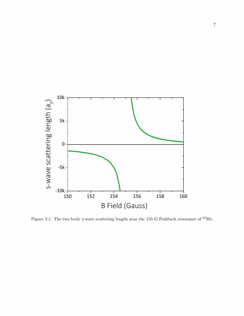
The strength of the interaction potential is defined by the s-wave scattering length, a. For low-

energy scattering, the scattering length is the distance from the origin at which the approximated

scattering wave function intercepts the x-axis [17]. A more intuitive picture of a is that it is the

radius of a “hard shell” that approximates the low-energy scattering of the atoms [22]. Near the

Feshbach resonance, a is described by

a(B) = abg

(1− ∆

B −B0

), (2.8)

where abg is the background scattering length, ∆ is the width of the resonance, and B0 is the

resonance position [23]. For the 85Rb resonance centered at B0 = 155.041(18) G, ∆ = 10.71(2) G

and abg = −443(3) a0 [24]. This 85Rb Feshbach resonance is plotted in figure 2.1.

The low-energy bound state that creates our Feshbach resonance is that of the Feshbach

molecule. The Feshbach molecule is a state where two atoms are weakly bound together, we

colloquially call this molecule a dimer. The energy of the Feshbach molecule is given by

Eb =−~2

ma2, (2.9)

where m is the mass of the 85Rb atom [21]. This binding energy is plotted in figure 2.2.

7

150 152 154 156 158 160-10k

-5k

0

5k

10k

B Field (Gauss)

s-w

ave

scat

terin

g le

ngth

(a0)

Figure 2.1: The two-body s-wave scattering length near the 155 G Feshbach resonance of 85Rb.

8

Figure 2.2: The blue line shows the calculated molecular energy for the Fesbach dimer, Eb. Thegreen line is the two-body scattering length.

9

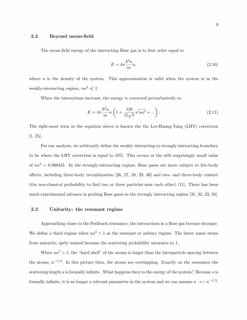
2.2 Beyond mean-field

The mean-field energy of the interacting Bose gas is to first order equal to

E = 4π~2a

mn, (2.10)

where n is the density of the system. This approximation is valid when the system is in the

weakly-interacting regime, na3 1.

When the interactions increase, the energy is corrected perturbatively to

E = 4π~2a

mn

(1 +

128

15√π

√na3 + ...

). (2.11)

The right-most term in the equation above is known the the Lee-Haung-Yang (LHY) correction

[1, 25].

For our analysis, we arbitrarily define the weakly interacting to strongly interacting boundary

to be where the LHY correction is equal to 10%. This occurs at the still surprisingly small value

of na3 = 0.000431. In the strongly-interacting regime, Bose gases are more subject to few-body

effects, including three-body recombination [26, 27, 28, 29, 30] and two- and three-body contact

(the non-classical probability to find two or three particles near each other) [11]. There has been

much experimental advance in probing Bose gases in the strongly interacting regime [31, 32, 33, 34].

2.3 Unitarity: the resonant regime

Approaching closer to the Feshbach resonance, the interactions in a Bose gas become stronger.

We define a third regime when na3 > 1 as the resonant or unitary regime. The latter name stems

from unitarity, aptly named because the scattering probability saturates to 1.

When na3 > 1, the “hard shell” of the atoms is larger than the interparticle spacing between

the atoms, n−1/3. In this picture then, the atoms are overlapping. Exactly on the resonance the

scattering length a is formally infinite. What happens then to the energy of the system? Because a is

formally infinite, it is no longer a relevant parameter in the system and we can assume a→∼ n−1/3.

10

The energy of the system can then be parameterized by the density,

En ≡ ~2(6π2n

)2/3/2m. (2.12)

Because the system is apparently defined solely by one parameter, we anticipate behavior that is

universal with density. Universal behavior in itself is exciting: other quantum degenerate universal

systems are high-temperature superconductors and neutron stars.

We can also define the momentum and time scales at which the system should evolve as

κn ≡(6π2n

)1/3, (2.13)

tn ≡ ~/En. (2.14)

The system’s quick evolution at resonance, with tn on the order to tens of microseconds for standard

condensate densities, complicates experiments. However for several years now experimentalists have

found novel solutions to overcome these obstacles. By studying post-resonance momentum genera-

tion, we have previously shown that degenerate Bose gases have a short-lived quasi-equilibrium state

on resonance [35, 36]. Other experiments have studied the perceived loss after a resonant Bose gas is

brought back to weak interactions [37, 38, 39], and most recently the two- and three-body contacts

of a resonant Bose gas were measured [40]. The fact that there are many theoretical predictions for

behaviors expected to emerge from many-body effects present in the resonant Bose gases has made

experimental progress in this regime a rewarding endeavor [41, 42, 43, 44, 45, 46, 10, 11, 12, 47, 48].

2.4 Beyond universality: Efimov trimers

Interactions become even more interesting when we look beyond two-body interactions to few-

and many-body interactions. The first step to this extension is the study of three-body interactions.

Three-body interactions were first studied by nuclear physicists to describe the interactions between

nuclei [49]. In particular, Vitaly Efimov derived the existence of an infinite series of three-body

bound states in 1970 [2, 3]. Each bound state is larger than the last by a scaling factor of eπ/s0 ≈

22.7, where s0 = 1.00624 [4, 50], and the binding energy E(p)T (p = 0, 1, 2...) is smaller by a factor of

11

22.72 [4, 9]. Efimov bound states are also considered “universal” - not because their energy depends

only on density, but because they have discrete scale-invariance, and the physics can therefore be

applied to a broad spectrum of physical systems.

Ultracold atomic physics experiments (in particular Boson experiments that, unlike their

Fermionic counterparts, are subject to three-body influence) have proven that Efimov bound states

exist as a bound three-atom molecule, called a trimer. These experiments have proven the existence

of Efimov states through observation of inelastic collision rates in atomic samples [51, 52, 34, 53,

54, 55, 56] and atom-dimer resonances [57, 58, 59, 60, 61], and observation of atomic loss after RF

association into Efimov states [62, 63, 64]. While these experiments send atoms into the Efimov

bound state, they do not directly observe the atoms in the Efimov bound state but instead surmise

their existence from loss rates of unbound atoms or two-body bound dimers. Very loosely bound

trimers have been observed in diffracted molecular beams of gaseous helium [65]. However, direct

observation of Efimov trimers in a cold, controlled gas has yet to be experimentally realized.

12

Figure 2.3: The solid and dashed red line represent the energies of the ground and first-excitedEfimov states, relative to three non-interacting atoms. These energies were calculated in the adia-batic hyper spherical representation [43, 8, 66]. Like the previous figures in this chapter, the blueline represents the energy of the Feshbach dimer plus one free atom, and the green is the two-bodyscattering length.

2.5 Experimental observations: loss rates

We discussed earlier how observing loss rates in both unbound atoms and two-body bound

dimers gives insight into the production of Efimov trimers. Loss rates are an invaluable tool for

ultracold gas experiments. They are simple to measure, as it is relatively easy to count the number

of atoms over time. The rate and spatial extent of the loss, however, gives rise to a plethora of

information as to the cause of the loss.

There are many mechanisms that can cause loss in a BEC. Of interest in our regime is three-

13

body recombination. Three-body recombination describes the event of three atoms colliding - two

of these atoms bond to form a molecule, and both the molecule and the third atom recoil with

kinetic energy gained from the new molecule’s binding energy [27]. This event results in overall

loss and heating of the condensate.

The three-body loss rate, Γ3, is defined by

N = −Γ3N. (2.15)

Γ3 is related to the three-body loss rate constant, L3 by Γ3 = L3〈n2〉, where 〈n2〉 is the density-

averaged square density, or∫n2(r) · n(r) d3r/N . In the zero-temperature, mean-field limit,

L3 ∼~ma4, (2.16)

therefore Γ3 ∼ n2a4 [67, 68, 27, 28, 29]. As a formally diverges on resonance, however, a plausible

physical limit is a ∼ n−1/3, yielding Γ ∼ n2/3 [69, 70]. This loss rate scaling at unitarity is consistent

with universal scaling with density.

At finite a however, the presence of Efimov states modulates the three-body inelastic collision

rates by a dimensionless log-periodic function of a [68, 27, 28, 4, 51, 52, 7, 71, 72, 21]. Because

Efimov states are still bound when 1/a → 0, it is not unreasonable to suspect that they may

influence the loss rates on resonance. Observation of an Efimov perturbation on the resonant loss

rates of a Bose gas would therefore demonstrate a breakdown of universal scaling with density in

the system.

The measurement of the three-body loss rate of a resonant Bose gas has been studied intensely

over the past several years [70]. The loss rates of a finite-temperature resonant Bose gas have been

measured in [37, 38, 39]. The loss rate of a zero-temperature resonant Bose gas was measured for

two densities in [35] and was found to be consistent with universal density scaling.

In Chapter 5 of this thesis we present a measurement of the apparent loss observed in a

1/a → 0, T → 0 Bose gas for densities ranging over two orders of magnitude. However, in

later chapters we explore how our measurement technique, which involves ramping back to weak

14

interactions before imaging, sweep our resonant atoms into weakly-bound molecules. Therefore the

observed loss is not solely a measurement of the resonant three-body loss rate, and may be even more

than merely the rate of the three-body loss summed with the production rate of shallow (weakly

bound) molecules. The evolution of the atoms’ propensity to be swept into shallow molecules occurs

simultaneously with the three-body loss to deeply-bound molecules. The questions that arise from

this entanglement are furthered following the revelation that the shallow molecules are a mixture

of both dimer and trimers. Strange effects seen for short evolution times even suggest that some

atoms may be in a superposition of dimer and trimer states.

Chapter 3

Imaging corrections

3.1 Review of previous imaging setup

The experiments written about in this thesis took place on an apparatus originally built by

Scott Papp [73]. This experiment used 87Rb to sympthathetically cool 85Rb into a BEC of around

70 × 104 atoms. Changes to this original set up include a nearly-spherical 10 Hz trap detailed in

[74], a high-intensity imaging setup detailed in [75], and a pair of Fast-B coils detailed in [36]. This

experiment is now dismantled, however a new and improved experiment is in the process of being

built to continue the resonantly interacting boson research this thesis explores.

In this chapter we discuss further changes made to the high-intensity imaging. These changes

enabled us to image the clouds in-trap and on resonance, thereby deducing how the density of a

resonant degenerate Bose gas changes on resonance. We will first review the high-intensity imaging

setup detailed in [75], then discuss why and what changes were necessary, and finally examine the

positive effects of these changes.

3.1.1 Absorption imaging: review

A very thorough review of absorption imaging can be found in [76]. Basically, incident light

shines on atoms, the atoms absorb the light thereby creating a shadow, and a camera down the

line images this shadow - we call this the shadow frame, IS . The cold collection of atoms are

“destroyed” by this process, meaning that they are heated enough that they leave, and probably

end up being adsorbed onto the walls of the science cell. After this destruction, a second, identical

16

light pulse is sent through the now empty science cell and imaged by the camera - we call this

the light frame, IL. Because our experimental set up is not perfect we also image a dark frame

(ID), where the camera takes an image with no incident laser light to collect information on the

background light and dark counts. By comparing the light and shadow frames (and subtracting

the dark frame from each), we deduce the measured optical depth (OD):

ODml = ln (Ii/If ) , (3.1)

where If ≡ IS − ID and Ii ≡ IL − ID. The peak optical depth (pkOD) is the largest optical depth

in the image, and occurs at the center of the cold cloud, pkOD = ODml(r = 0). We generally fit

our OD with a 2D Gaussian fit with an amplitude of pkOD and x and y sizes of σx and σy. When

the frequency of the imaging laser is on resonance with the atomic transition (i.e. zero detuning),

the number of atoms in the cold cloud is then

N =2π

σ0· pkOD · σxσy, (3.2)

where σ0 is the resonant cross section, = 3 × 780 nm / 2π, and σx and σy are the axial and radial

cloud sizes defined by a 2D Gaussian fit[76].

Optical depth is a very useful term but the word is used in variety of manners. For clarity,

we define several OD’s that will be used throughout this chapter. The actual optical depth of

our cloud is ODreal, defined by the density integrated along the imaging direction,∫ndz. The

maximum value of ODreal occurs at the center of the cloud, pkOD = ODml(r = 0). If our imaging

set up had perfect polarization, zero detuning, and all around perfect imaging, the intensity of the

shadow frame would be reduced by Is = ILe−ODreal . In equation (3.1) we defined the measured

OD, defined by the amount of missing light (ml) in the shadow image. This is the standard optical

depth measurement, but it is affected by bad polarization, laser detuning, and saturation. We

use the value of ODmax to determine the amount “bad light” (e.g. light with bad polarization

or frequency) in our system, ODmax ≡ ODml in the limit of ODreal → ∞. We later define an

ODhigh in equation (3.3) that overcomes the saturation limitations of ODml and therefore enables

17

measurements of large (high) optical depths. ODhigh is a good approximation for ODreal when the

detuning is zero, the polarization is pure, and ODreal is below 15.

The camera we use to image this laser light is a Roper Scientific (Model 1024B) with

1024x1024 pixels that are each 13 µm wide per side. The camera is back illuminated to ensure high

quantum efficiency of 72%, meaning that 0.72 electrons are emitted for each photon. The least

significant bits (LSB) per electron of the camera was measured on April 27 2010 (before my time)

to be 0.96 ± 0.1 electrons/ct.

We use a two-lens telescope to magnify our images before the camera. The first lens is f = 8

cm located about 8 cm away from the atoms, the second a f = 18 cm lens about 18 cm away from

the camera. The magnification of this lens system is 2.25. This results in a pixel-to-size calibration

of 5.8 µm/px. This calibration was measured to be pxcalib = 5.7 µm/px by imaging untapped

falling atoms and comparing their acceleration to that of gravity.

The resolution of this system was calculated (by measuring the expansion of the cloud under

known conditions) to be 1.07 and 1.14 pixels in the x and y directions, respectively. This corresponds

to a resolution of 6 and 6.5 µm. The diffraction-limited resolution of our lens system is only 1.05

µm [77]. Our actual resolution is so much larger because of spherical aberrations, more on this in

the next section.

3.1.2 High-intensity imaging: review

There is a maximum intensity of incident light beyond which the atom’s absorption begins to

saturate, see [75] for more thorough explanation of this saturation. We account for this saturation

by defining a new, high-intensity OD:

ODhigh = ln (Ii/If ) +Ii − IfIsat

(3.3)

[78]. Isat was measured for 85Rb to be 1.669 mW/cm2 for the |3,−3〉 → |4,−4〉 transition [79]. For

our purposes it is easier to define the effective Isat in our system,

Ieffsat =

α · T · Isat · t · pxcalib2

Cpp · h · ν, (3.4)

18

where α = 2 to account for our polarization axis (see figure 3.1), T = 53.4% is the transmittance

through the camera ND filter, Cpp is the quantum efficiency of our camera (0.72 electrons/photon)

divided by the measured LSB/e− (0.96 electrons/ct) = 0.75 counts per photon, t is the length of

the imaging pulse (normally 50 µs for low-intensity imaging, and 5 µs for high-intensity imaging)

and ν is the frequency of our laser, given by c/λ = c/780.24 nm ≈ 384.2 THz. Ieffsat for our system

is calculated to be 8730 light counts.

We measure Ieffsat by imaging clouds (with an actual OD of ODreal) with different amounts of

incident light (IL) and comparing to the ODml. Ieffsat relates these quantities by

IL =ODreal −ODml · Ieff

sat

1− e−ODml. (3.5)

We find that the measured value of Ieffsat appears to change with the actual optical density of

the cloud, ODreal. This was because optical depth saturation is also affected by bad light, i.e. light

Figure 3.1: When taking an image of the cloud in-trap, we have the Bias coils define the quantizationaxis. This axis is perpendicular to the incident light. Because the incident light is linearly polarized,half of the light can be absorbed by the atoms, the other half cannot. We account for this byincluding a factor of 2 in our OD calculations.

19

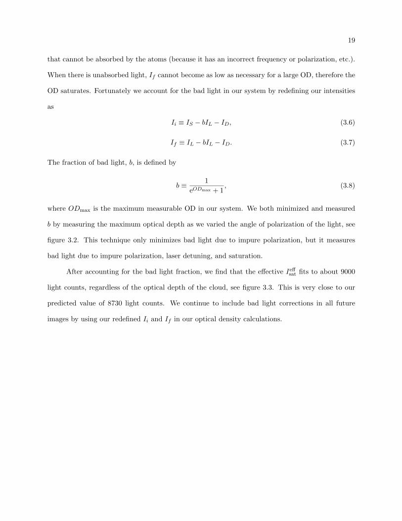
that cannot be absorbed by the atoms (because it has an incorrect frequency or polarization, etc.).

When there is unabsorbed light, If cannot become as low as necessary for a large OD, therefore the

OD saturates. Fortunately we account for the bad light in our system by redefining our intensities

as

Ii ≡ IS − bIL − ID, (3.6)

If ≡ IL − bIL − ID. (3.7)

The fraction of bad light, b, is defined by

b ≡ 1

eODmax + 1, (3.8)

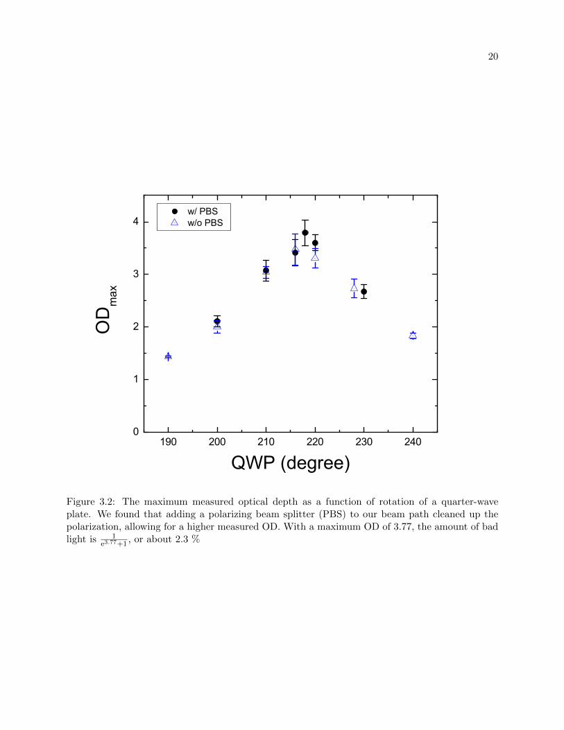
where ODmax is the maximum measurable OD in our system. We both minimized and measured

b by measuring the maximum optical depth as we varied the angle of polarization of the light, see

figure 3.2. This technique only minimizes bad light due to impure polarization, but it measures

bad light due to impure polarization, laser detuning, and saturation.

After accounting for the bad light fraction, we find that the effective Ieffsat fits to about 9000

light counts, regardless of the optical depth of the cloud, see figure 3.3. This is very close to our

predicted value of 8730 light counts. We continue to include bad light corrections in all future

images by using our redefined Ii and If in our optical density calculations.

20

190 200 210 220 230 2400

1

2

3

4 w/ PBS w/o PBS

OD

max

QWP (degree)

Figure 3.2: The maximum measured optical depth as a function of rotation of a quarter-waveplate. We found that adding a polarizing beam splitter (PBS) to our beam path cleaned up thepolarization, allowing for a higher measured OD. With a maximum OD of 3.77, the amount of badlight is 1

e3.77+1, or about 2.3 %

21

0 1 2 3 4 5 60

10k

20k

30k

40k

50k Isat 9020 ± 590OD

real 15180 ± 210

ODreal 2

3180 ± 150OD

real 31188 ± 67

light

cou

nts

ODml

Figure 3.3: To measure Ieffsat, we observed the measured ODml for various incident light counts for

clouds of three different intrinsic ODreal, about 1200, 3200, and 5200 mOD. The y-axis on this plotis the independent variable, the x-axis dependent. When account for a bad light fraction of 2.3%,we see Ieff

sat fits to 9020(590) light counts, in good agreement with our expected value of 8730.

22

3.2 New imaging system

3.2.1 Reasons to upgrade

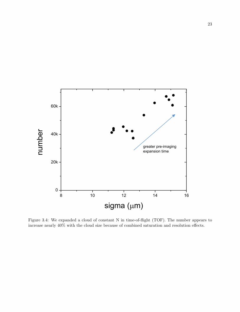
There are many possible experiments that require imaging on resonance (and therefore in

trap) to better understand the resonantly interacting Bose gas. Our original resolution of 6 µm

seems at first good enough to image our 30 µm diameter in-trap cloud size. However, when a cloud

is both small and optically dense, we observe a stifled optical depth measurements (figure 3.5)

along with a larger cloud size, as if the resolution were changing. This is because our high-intensity

saturation corrections break down near the resolution limit. This results in the number appearing

to increase with the time-of-flight (TOF) expanded clouds, see figure 3.4.

23

8 10 12 14 160

20k

40k

60k

number

sigma ( m)

greater pre-imagingexpansion time

Figure 3.4: We expanded a cloud of constant N in time-of-flight (TOF). The number appears toincrease nearly 40% with the cloud size because of combined saturation and resolution effects.

24

0 5 10 15 20 250

2

4

6

8

10

pkOD

expansion time (ms)

Figure 3.5: The measured pkOD as a function of cloud size for a cloud of constant N. The peak ODshould decrease as the cloud expands, however it does not because the measured OD is saturatedaround 8, when it should be nearly 20 for the smallest cloud size (corresponding to least expansiontime).

25

Figure 3.6: An unexpanded BEC of 70k atoms at 150 a0 should have a pkOD of 25 and a fittedGuassian size (sigma) of 8 µm. (a) In our old imaging system this cloud was measured at 10.8µm sigma and peak OD of 8.8, resulting in a number of 45k. (b) In the new imaging system wemeasure a sigma of 8.6 µm and a peak OD of 20, resulting in a calculated number of 63k.

3.2.2 New imaging lenses

The resolution of our old imaging system was limited by aberrations, specifically due to

spherical aberrations, imperfect tilt and alignment, and small magnification [77]. As we saw in the

previous section, this resolution worsened when we combined large optical depths with small cloud

sizes near the resolution limit. We therefore sought to improve our imaging resolution. Counter-

intuitively, we actually increased the diffraction-limited resolution (given by 0.61 λd/r, where λ

is the laser wavelength, d is the distance between the lens and the object, and r is the radius of

the lens) by decreasing the radius of both the objective and imaging lenses to a half inch. This

improved our overall resolution by decreasing the aberrations caused by tilt and misalignment.

The new lenses are spaced 10mm apart and have focal lengths (f) of 75 and 500mm, resulting in

a magnification of 6.35, see figure 3.6.

This new lens system increases our diffraction-limited resolution to 1.96 um. Our actual

measured resolution is close to the diffraction limit, at 2.2 +/- 0.1 µm. This is why we see diffraction

rings (an airy disc pattern) around our smallest clouds, see figure 3.7. We measured the resolution by

26

making the smallest cloud possible at a = 6±2 a0, where the cloud size is set by the trap frequency,

σreal = 3.9 and 3.6 µm in x and y. σmeas was 4.206±0.98 and 4.20±0.94, so our resolution is then√σ2meas − σ2

real = 2.27± 0.01 and 2.09± 0.01. We calibrate the magnification of this system with

respect to the camera pixel size by watching the cloud fall and find it to be pxcalib = 1.996 ± 0.002

µm/px.

Because of the larger magnification, we can now throw more incident light onto our conden-

sate. Our camera pixels saturate about 65k light counts, so we aim to keep the laser light at or

below 50k light counts. 50k light counts corresponded to only 0.5 mW of incident light on the

atoms with our previous magnification (when t = 5µs, constant for all future experiments). With

our new magnification that same amount of incident light expands to only 7k light counts per pixel

at the camera. We can therefore increase the incident light to 2 mW before the camera pixels

near saturation. Increasing the amount of light incident on the atoms improves the maximum

measurable pkOD and reduces saturation effects. We were unable to measure the Ieffsat of the new

Figure 3.7: We created a very small cloud at a = 6 ± 2 a0. On the right are the x and y cross-sections across the center of the cloud, the red lines are the data, the blue a Gaussian fit. Thereare visible diffraction rings, or Airy discs, around this cloud because we are near the diffractionresolution limit. The size of this cloud is set by the harmonic oscillator length of our harmonictrap, aosc = 3.9(3.59) µm in the x(y) imaging directions. By comparing this predicted size to themeasured size we deduce an average resolution of 2.2 ± 0.1 µm.

27

Figure 3.8: Because the magnification of our system has changed, Ieffsat also changes. We sought

to measure Ieffsat at several optical depths, however dependencies between Ieff

sat and OD dramaticallyincreased the error bars. We do see that an Ieff

sat of about 900 light counts produces good fits,believable OD values, and is close to our predicted value of 1074 light counts.

lens system because of dependencies in the fitting function between OD and Isat. We did see that

an average fit of 900 light counts (see figure 3.8) produced good fits, believable OD measurements,

and was very close to our prediction of 1074. The fractional intensity of the incident light, I/Ieftsat,

is therefore over 50, a very good ratio when using high-intensity imaging.

3.2.3 De-mag system

While the large magnification of the new lenses means that we can now measure a very small,

optically dense cloud, it also means that we can no longer image very large clouds. Of particular

interest for apparatus-tuning and debugging purposes is imaging the hot 87Rb cloud suspended

in the magnetic trap during the initial evaporation stages - this cloud could be up to 400 µm in

Gaussian σ. To accommodate this large cloud we implemented de-mag lenses into our imaging

system. The de-mag lenses are two additional lenses that can be flipped into the imaging beam

path, see figure 3.9. The de-mag lenses are 2 inches in diameter with focal lengths of 100 and 60

mm.

With the de-mag system in place, the total magnification of the system is expected to be 1,

therefore pxcalib should be 10.25 µm/px. We measured this as 10.5 µm/px by measuring the same

cloud with both the de-mag system in and out of the system, see figure 3.10. See [77] for more

28

Figure 3.9: The de-mag lenses (in blue) are two large lenses that when flipped into the imagingbeam path reduce the magnification from 6.35 to 1. Not to scale, figure borrowed from [77].

information on the de-mag lens system.

29

Figure 3.10: The same cloud imaged with and without our de-mag lenses. (b) Without the de-maglenses the measured cloud size is 142.5 and 122.5 px in x and y, corresponding to 285 and 245 µm.(a) With the de-mag lenses the measured cloud size is 27.1 and 23.25 px, corresponding to a 10.5µm/px calibration.

3.3 New OD range and expansion data

With our new imaging system (sans de-mag lenses) we find that the number no longer changes

with sigma for most cloud sizes, see figure 3.11. This is because the measured optical depth (ODhigh)

is no longer saturated at 8, and can increase with smaller cloud sizes (smaller expansion times),

up to about 20, see figure 3.12. We do see a 10% reduction in cloud size when the optical depth

is above 15, we therefore conclude that we can trust our new imaging system up to clouds with

optical depths up to 15.

30

8 9 10 11 12 13 14 15 160

20k

40k

60k

80k

ARP no poof

num

ber

sigma ( m)

Figure 3.11: The measured number as a function of cloud size - the number of each cloud is heldconstant while the cloud size is expanded with TOF imaging. This atom number is transferredto the imaging state with a 9 dBm microwave pi-pulse. We compare this number to a cloudtransferred to the imaging state with an ARP, the green line, our trusted “real number”. We seethat the number no longer changes significantly with size. except by about 10% at the smallestsizes. These data correspond to the ODreal 15, we therefore conclude that we can trust our newimaging system up to optical depths of 15.

31

0 10 200

5

10

15

20

peak

OD

expansion time (ms)Figure 3.12: With our new imaging lenses we see that for a constant-N cloud the peak optical depthchanges with cloud size, as expected! This measured optical depth reaches a maximum value of 20,the expected value given the cloud size. This data is the same data as plotted in 3.11 However, thedata below 5 ms expansion time correspond to a peak OD greater of equal to 15, and this resultsin a reduced measured number of about 10%. Therefore we only trust our new cloud images up toa peak optical depth of 15.

32

3.4 Imaging analysis

In addition to correcting for the effective saturation intensity and the small percentage of bad

light in our system, there is a third imaging systematic in need of correction: uneven probe pulses,

i.e. the light and shadow frames having not exactly the same amount of light. This effect is caused

by the AOM warming up - a warm AOM has slightly better alignment than a cold AOM. This is

a problem because the incident light on the atoms is not constant across the imaging frame, see

figure 3.13(a). Therefore when we subtract the shadow frame from the light frame, we see small

remnants of this laser pulse in the background, when we should only see the round atom shadow,

see figure 3.13(b).

Figure 3.13: (a) the light frame, IL. (b) the light frame minus the shadow frame, IL − IS. Thedark red spot is a cloud of atoms while the remaining light stuff is laser remnants caused by theincreased incident light in the light frame. We also see fringes across this frame subtraction becausethe two frames do not completely overlap - the small change in position is due to shaking optics,most likely caused by the cart, a coil that physically moves across our table to transport our atomsto the science cell.

3.4.1 Epsilon correction

Rather than correct this systematic by altering the AOM output, we find it easier to account

for it during post-imaging analysis. The variation in incident laser light varies by, on average, only

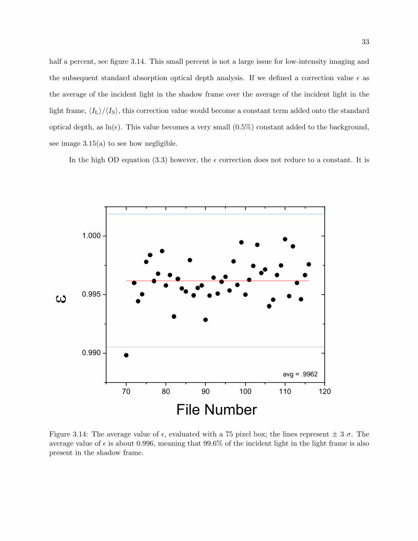
33

half a percent, see figure 3.14. This small percent is not a large issue for low-intensity imaging and

the subsequent standard absorption optical depth analysis. If we defined a correction value ε as

the average of the incident light in the shadow frame over the average of the incident light in the

light frame, 〈IL〉/〈IS〉, this correction value would become a constant term added onto the standard

optical depth, as ln(ε). This value becomes a very small (0.5%) constant added to the background,

see image 3.15(a) to see how negligible.

In the high OD equation (3.3) however, the ε correction does not reduce to a constant. It is

70 80 90 100 110 120

0.990

0.995

1.000

avg = .9962

File NumberFigure 3.14: The average value of ε, evaluated with a 75 pixel box; the lines represent ± 3 σ. Theaverage value of ε is about 0.996, meaning that 99.6% of the incident light in the light frame is alsopresent in the shadow frame.

34

Figure 3.15: (a) The OD from the from figure 3.13 evaluated using equation 3.1; the laser remnantsare too small to discern. (b) The OD from the same figure now evaluated using equation 3.3 - nowthe background becomes significant.

correctly accounted for in the optical depth as

OD ≈ ln

(ε IiIf

)+ε Ii − IfIeff

sat

, (3.9)

If ε is far from 1 and not correctly accounted for, a large non-linear background appears, see figure

3.15(b). To account for (remove) this background, we measure ε for each shadow/light frame pair.

Because the shadow frame has a dark spot due to the atoms, taking an average over the

entire frame would incorrectly result in a much lower average light count for the shadow frame. We

therefore define a box around the center of our cloud and only consider the light counts outside of

this box. If this box too small, we might artificially lower ε by including atom dark spots; if this

box too large, there will be too little incident light to calculate a trustworthy ε, see figure 3.16(a)

and (b) for an example of each of these situations. We find that a box size of 75 pixels is best, see

figure 3.16(c). Note that these pixel values were determined with the old imaging system, and the

box size was adequately adjusted with the new imaging magnification.

To best illustrate how correction with ε improved our images, we need to define cumulative

distribution functions (CDFs). CDFs are generated by azimuthally averaging the optical density

35

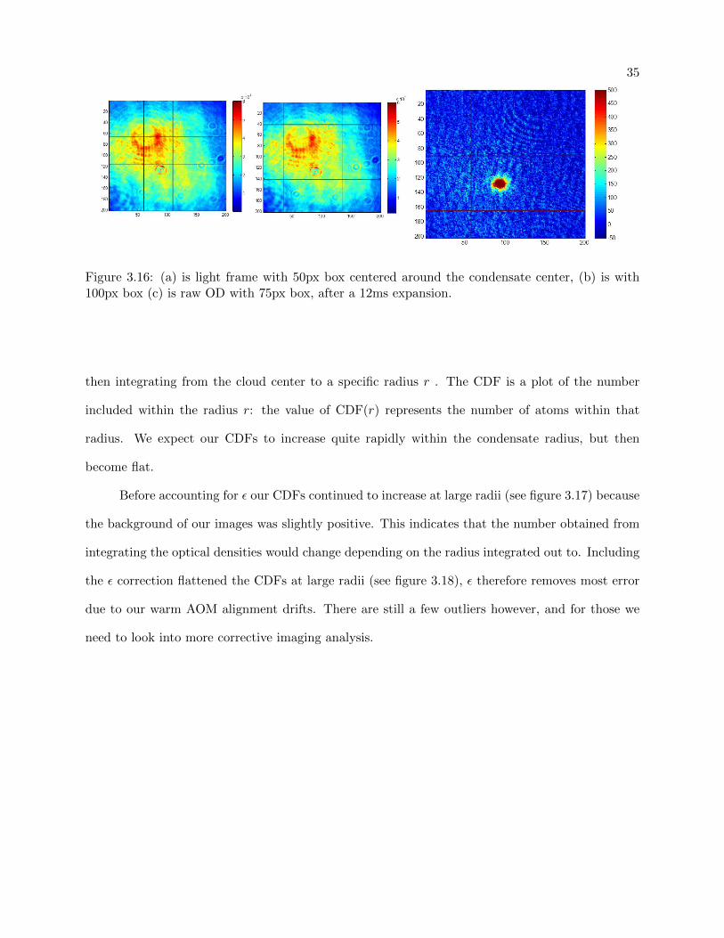
Figure 3.16: (a) is light frame with 50px box centered around the condensate center, (b) is with100px box (c) is raw OD with 75px box, after a 12ms expansion.

then integrating from the cloud center to a specific radius r . The CDF is a plot of the number

included within the radius r: the value of CDF(r) represents the number of atoms within that

radius. We expect our CDFs to increase quite rapidly within the condensate radius, but then

become flat.

Before accounting for ε our CDFs continued to increase at large radii (see figure 3.17) because

the background of our images was slightly positive. This indicates that the number obtained from

integrating the optical densities would change depending on the radius integrated out to. Including

the ε correction flattened the CDFs at large radii (see figure 3.18), ε therefore removes most error

due to our warm AOM alignment drifts. There are still a few outliers however, and for those we

need to look into more corrective imaging analysis.

36

Figure 3.17: The cumulative distribution functions (CDFs) of many condensates after a 5-100-5 µsresonance jump. The clouds were expanded in TOF for 6 (blue), 12 (red) or 24 (green) ms. Withno ε correction, we see that the CDFs continue to increase at large radii, indicating that the opticaldensity images have a positive background.

37

Figure 3.18: The same data that was presented in the previous figure, but analyzed with theε correction. The ε correction enables the CDFs to flatten at large radii, indicating an opticaldensity background of zero. There are minimal outliers after the ε correction that still have non-zero background.

38

3.4.2 Residual background subtraction

The ε correction does not zero-out the background of all images. Plotting more CDFs, we

see that maybe 5% do not have zero slopes are large radii, see figure 3.19. We find that the images

not corrected by ε tend to have large fringes in their frames, which may skew the ε calculation.

Figure 3.19: More cumulative distribution functions of condensates after various resonance jumpsand TOFs. We see that maybe 5% of the CDFs continue to have a non-zero background after theε correction. We expect these data to have varying total number, this is not noise.

39

Figure 3.20: The fitted values of the residual background (B.G.) for various file numbers. Theblue, purple, and green points correspond to TOFs of 6, 12, and 24 ms. Larger expansion timeshave larger cloud sizes and smaller optical depths. The fitted residual background appears to beindependent of the cloud size and optical depth, and appears to be random noise.

We fit these CDFs at large radii with

N + B.G. · r2, (3.10)

where N is the fitted atom number and B.G. is the fitted slope defining the residual background.

The residual background fits have a standard deviation of 0.18, see figure 3.20. Subtracting the

fitted residual background from the OD drastically improves the flatness of the CDF at large radii,

see figure 3.21, and works nearly consistently for all images, see figure 3.22.

To measure the number of atoms in our system, we could integrate the optical depth out to a

certain radius - this is equivalent to a single point of CDF(r). However, there are small wiggles in

our CDFs due to the OD fringes, these wiggles translate into number noise that varies with r. We

40

find that the fitted number N from equation 3.10 has much less noise than the integrated number,

see figure 3.23. We therefore use the fitted N to define the atom number in all future resonant

measurements.

It is worth mentioning that later in this thesis we begin imaging molecules. As the molecular

clouds have much lower optical depth, we do not use high-intensity imaging, and therefore the

ε correction is not necessary. We found no significant different in our molecule number when

azimuthally averaging the data and fitting N with the residual background as compared to taking

N from a 2D Gaussian fit, and we therefore use the latter (simpler) approach to define molecule

Figure 3.21: Subtracting out the residual background of the original CDF (blue) results in a CDFthat is much flatter at large radii. This particular CDF is of a non-resonant condensate expandedfor 6 ms TOF.

41

Figure 3.22: CDFs from the same condensate images as figure 3.20. We subtracted the fittedresidual background (B.G.) from the optical depth for each CDF. This results in the outlier CDFsfinally flattening at large radii.

number in all future resonant measurements.

42

0 200 400 600 8000

20k

40k

60k

80k

100k4 March 2015

n: 5ish E12/ccramp: 5-dwell-5 usfield: 163 GRF: ARP (2ms)

9 dBm, N/A, no

number

dwell time ( s)

CDF fit Integral

Figure 3.23: The number of atoms as a function of dwell time at unitarity after evaluated byradially integrating optical density (green triangles) or CDF fit using equation 3.10 (pink points).The latter technique reduces the noise due to background fringes.

Chapter 4

Density

Most of the experiments discussed in this thesis involve ramping to resonance, allowing the

system to evolve on resonance, then ramping back out to weak interactions. Details of these ramps

and definitions of the time scales used to characterize the experiment are discussed in Chapter 5.

In these experiments we vary many knobs, including the resonant evolution times, the ramp in /

out times, and the initial density of the gas. The density of the gas changes on resonance, due to

both loss and expansion. We therefore always report the “initial” density, meaning the density of

the condensate just before we begin the sweep to resonant interactions. We reference this density

in units of E12/cc, more commonly seen as ×1012 cm−3. In this chapter we discuss how we vary

the initial density of our system by over two orders of magnitude.

4.1 Density-averaged density

When we colloquially say density (n), we are referring to the density-weighted density, i.e. the

density averaged by the density distribution. The density of our harmonically trapped condensate

varies from a peak density (npk) at the center to 0 at the very edges. Other ultracold atomic

experiments avoid this large variation in density by either a box trap [80] or a donut beam [81].

We calculate the relation between the density-weighted density and peak density for a con-

densate in a spherically symmetric harmonic trap of frequency ω. Because the number of atoms in

our condensate is large, we use the Thomas-Fermi approximation to describe the wave function of

44

our system as

ψ(r) =

√µ− V (r)

U0, (4.1)

where µ is the chemical potential given by ~ω2

(15N a√~/(mω)

), V (r) is the harmonic trapping potential

equal to mω2 r2/2, and U0 is the interaction energy, 4π a ~/m [17]. The peak density occurs at the

center of this wave function, npk = |ψ(0)|2 = µU0

. The size of a Thomas-Fermi condensate, defined

where V (r) = µ, is called the Thomas-Fermi radius and is given by RTF =√

2µmω2 [17].

The density-weighted density is defined as

〈n〉 ≡∫n2(r) d3r∫n(r) d3r

. (4.2)

This can be rewritten as

〈n〉 =

∫|ψ(r)|4 d3r

N. (4.3)

Plugging in equation 4.1 to equation 4.3 and evaluating the integral from 0 to RTF yields

〈n〉 =4

7

µ

U0. (4.4)

We therefore conclude that for a harmonically trapped Thomas-Fermi condensate, 〈n〉 = 47 npk and

is related to ω, N , and a by

〈n〉 =(15Na)2/5

14π a

(mω~

)6/5. (4.5)

.

4.2 Perez-Garcia model

We change the density over two orders of magnitude by changing the size of our condensate.

We vary the size of our condensate by jumping the scattering length to larger or smaller values

(ajump). This sudden change in interaction strength causes the atoms to either push away from or fall

towards each other. When the cloud is in a harmonic trap, this sudden change in scattering length

induces an oscillatory size change called a breathe. The dynamics of these breathes are modeled

45

using a variational technique to solve the Gross-Pitaeveskii equation in [82]. In the case of positive

scattering lengths they derive an analytic solution describing the axial and radial condensate widths:

wr + f2r wr =

~2

m2

(1

ω3r

+

√2

π

aN

w3r wz

), (4.6)

wz + f2z wz =

~2

m2

(1

ω3z

+

√2

π

aN

w2r w

2z

), (4.7)

where wi relates to the 2D Gaussian-fit widths by wi = σi/0.78. We call these equations the

“Perez-Garcia model”.

The three trapping frequencies of our nearly symmetric trap were measured to be 10.46, 9.47,

and 10.56 Hz, see figure 4.1. We therefore set our radial and axial trapping frequencies (fr and

fz) to 10.5 and 9.5 Hz, and this predicts a breathing oscillation period (roughly a half-trap cycle)

of about 44 ms. We can therefore expand or contract our cloud by jumping the field to larger or

smaller ajump and allowing the cloud to breathe for a quarter trap cycle (i.e. 22.5 ms), at which

point the size reaches a maximum or minimum, see figure 4.2. We will now explore the limitations

of this method in both the high and low density limits.

46

Figure 4.1: We measured the magnetic trapping frequencies by purposefully loading our cloud froma misaligned optical trap to induce a slosh. We add or subtract the measured z and y cloud centersbecause the axes of our trap are 45 degrees from our imaging axes [74]. We measure trappingfrequencies of 10.46(9), 9.47(14) and 10.56(0.18) Hz. These trap frequencies were measured severalyears earlier in [74] to be 10.41(4), 9.39(7), and 10.21(5), and have not drifted significantly.

47

Figure 4.2: The predicted axial size of a condensate in a 9.5 x 10.5 Hz as a function of time afterjumping to 500 a0 at time 0. The cloud returns to its original size around 44 ms (equal to a half-trapperiod) and reaches a maximum size around 22 ms.

48

4.3 High density limit

High densities are achieved when ajump < ai. We measure ajump to within ∼ 5 a0 using

microwave spectroscopy. This uncertainty is fine for large values of ajump, however when a becomes

on the order of 5 a0 itself, it transfers into large uncertainties in density. We therefore set our

minimum ajump to 15 a0, for which we expect densities of over 12 times our original density.

The real limitations on our high density however come from the speed of our fast-B coils.

As will be explored in Chapter 5, our fast-B coils ramp our condensate to and from resonance and

have a maximum speed of about 8 Gauss in 5 µs. More importantly, the fast magnetic ramps have

a turn-around time that sets the minimum time spent on resonance to about 10 µs (this minimum

time depends on the density of the cloud, as resonance is defined by na3 > 1). For experiments in

which we want to set tdwell ∼ 1 tn, this sets our maximum density to about 60 E12/cc, where tn is

11.5 µs.

4.3.1 Actual high density limit

We want to image the clouds in trap to compare their sizes to the predicted values to ensure

that the density is changing as expected. However, the smaller sizes of the high density clouds

make it difficult to image without expansion. So we instead jump back to ai and allow the cloud

to expand before imaging. We are therefore comparing our clouds to a two-jump Perez-Garcia

prediction, see figure 4.3. The accuracy of the high density predictions is limited by trap frequency

uncertainties, as ω becomes more important in equations (4.6) and (4.7) at low a. Based on the

measurement comparisons in figure 4.4, we can trust that our high density clouds are correct when

we jump down to as low as 19 a0. This corresponds to a density of 35 E12/cc.

49

0 10 20 30 40 504

6

8

10

12

14

(px)

time (ms)

Figure 4.3: After creating a condensate at ai = 146.25 a0, we jump to a = 54.71 a0 at t = 0 ms andallow the cloud to compress to high density over a quarter trap period. Because the high densitycloud is difficult to reliably image, we then jump back to ai to expand the cloud for another 22.5 ms.The black points represent measurements of our condensate size, in 2D Gaussian σ, at 0 time andat 45 ms, transferred to the imaging state with a microwave π-pulse . The solid line represents theexpansion predicted by the Perez-Garcia model. We see good agreement between the predictionsand our measurements.

50

0 20 40 60 80 100 120 1405

10

15

20

adju

sted

siz

e (

m)

ajump (a0)

measured x (1.5px resolution excluded)

PG axial PG radial

original size

Figure 4.4: The black points represent the adjusted (i.e. resolution subtracted) measured size, in2D Gaussian σ, at t = 45 ms after an ai → ajump → ai jump sequence with quarter trap expansions,where ai is 122.6 a0. The green and pink triangles represent the axial and radial predictions fromthe Perez-Garcia model. The points at 122.6 a0 are the original cloud size (no jump to 500 a0). Wesee good agreement with the model when jumped to as low as 19 a0, with only minor discrepanciesin cloud size beginning to emerge.

51

4.4 Low density limit

The density is lowered when ajump < ai. There are two mechanical limitations to our lower

density: the magnetic field gradient and heating of the Fast-B coils. There is also an interaction-

based limit that we extend by a double-jump method.

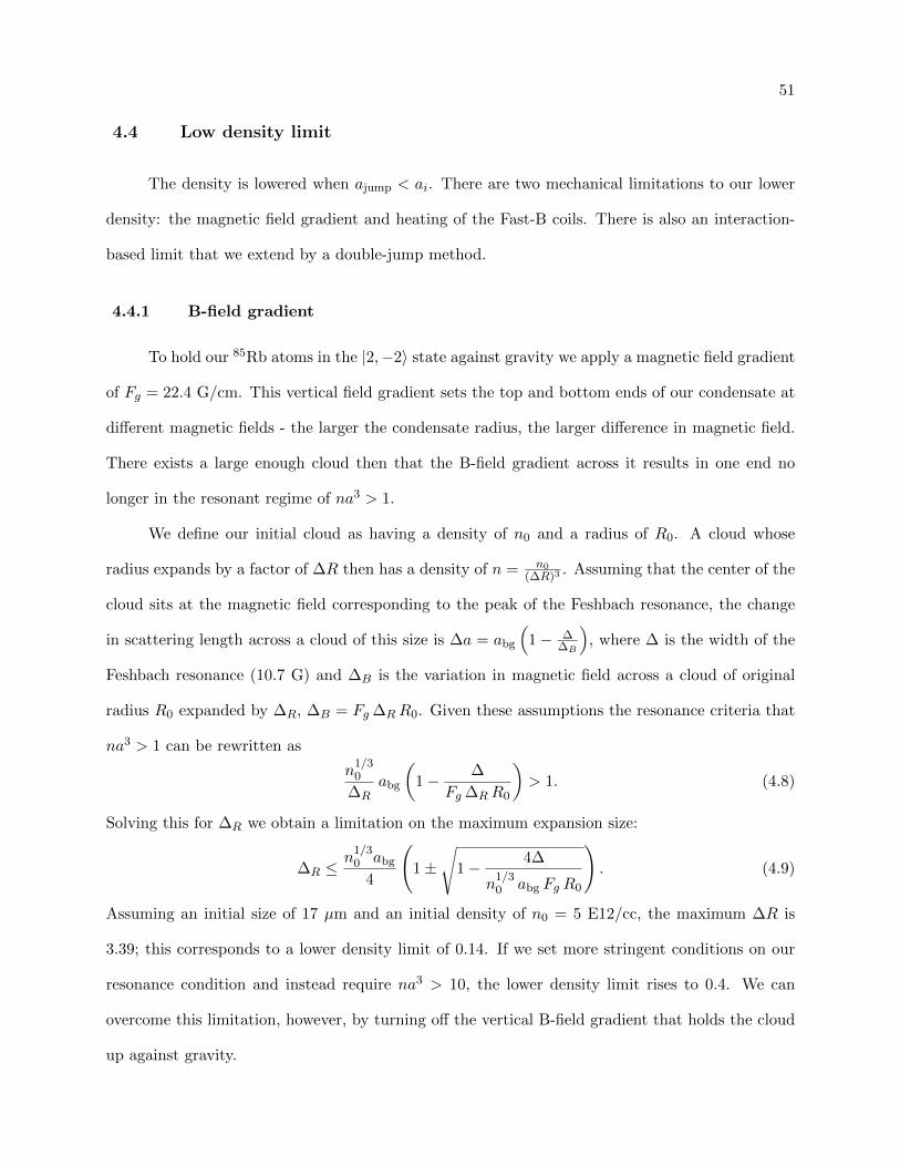
4.4.1 B-field gradient

To hold our 85Rb atoms in the |2,−2〉 state against gravity we apply a magnetic field gradient

of Fg = 22.4 G/cm. This vertical field gradient sets the top and bottom ends of our condensate at

different magnetic fields - the larger the condensate radius, the larger difference in magnetic field.

There exists a large enough cloud then that the B-field gradient across it results in one end no

longer in the resonant regime of na3 > 1.

We define our initial cloud as having a density of n0 and a radius of R0. A cloud whose

radius expands by a factor of ∆R then has a density of n = n0(∆R)3 . Assuming that the center of the

cloud sits at the magnetic field corresponding to the peak of the Feshbach resonance, the change

in scattering length across a cloud of this size is ∆a = abg

(1− ∆

∆B

), where ∆ is the width of the

Feshbach resonance (10.7 G) and ∆B is the variation in magnetic field across a cloud of original

radius R0 expanded by ∆R, ∆B = Fg ∆RR0. Given these assumptions the resonance criteria that

na3 > 1 can be rewritten as

n1/30

∆Rabg

(1− ∆

Fg ∆RR0

)> 1. (4.8)

Solving this for ∆R we obtain a limitation on the maximum expansion size:

∆R ≤n

1/30 abg

4

(1±

√1− 4∆

n1/30 abg Fg R0

). (4.9)

Assuming an initial size of 17 µm and an initial density of n0 = 5 E12/cc, the maximum ∆R is

3.39; this corresponds to a lower density limit of 0.14. If we set more stringent conditions on our

resonance condition and instead require na3 > 10, the lower density limit rises to 0.4. We can

overcome this limitation, however, by turning off the vertical B-field gradient that holds the cloud

up against gravity.

52

4.4.2 Fast-B heating

The second mechanical limitation to our low density achievements is the heating of the Fast-B

coils. A little more than 8 Amps of current is required to jump our field from ai to 1/a→ 0. Unlike

the IP and bias coils, the fast-B coils are not water-cooled. We therefore have limited time before

the coils heat enough to warp our science cell or cause general mayhem. The fast-B coils have

a resistance of about 0.018 Ohms, this generates 1.2 Watts with 8.2 Amps. This corresponds to

about a heating of about 6.7 deg C after a 1 second pulse. We use a very conservative estimate of

keeping the cumulative temperature below 5 deg C when experiments are repeated on a 90 second

duty cycle in a confined environment (i.e. little air flow). This limits the amount of time the fast-B

coils can be running at full current to about 2 ms. If one is doing an experiment with dwell times

of about 1 tn, this limits the lower density to about 0.03 E12/cc.

4.4.3 Lee-Huang-Yang limit

Ultimately our low density achievements are limited by interactions, specifically when the

interactions increase out of the mean-field limit. When we first jump to a large scattering length,

both the density and scattering length are not small and therefore na3 can be large. This is a

problem because a large na3 is indicative of strong interactions in the system, and these strong

interactions could modify the energy of our system. We want to keep our cloud in the weakly-

interacting regime, where losses and interactions are minimal. We define the weakly-interacting

regime as where the Lee-Huang-Yang (LHY) correction to the energy density is below 10 %. The

LHY correction was discussed in detail in Chapter 2 and the first order term was

128

15√π

√na3. (4.10)

The correction term is equal to 10% when na3 is equal to 0.000431.

We see that when we jump our cloud from its initial ai = 150 a0 to ajump = 2000 a0, the LHY

correction jumps up to as high as 38% and remains above 10% for nearly 10 ms, see figure 4.5.

During this time there may be significant heating in the cloud, as well as loss due to three-body

53

recombination. The largest scattering length that we can jump with our initial density cloud while

keeping the LHY correction below 10% is 780 a0. After 22 ms expansion at 780 a0, the cloud

density will fall to only 0.71 E12/cc. While this is a lower density than our original density, it is

preferable to reach even lower densities.

Figure 4.5: (a) Our original method to create a low density cloud involved jumping to a singlelarge scattering length. To achieve a density of 0.195 E12/cc, ajump = 2000 a0 for 22 ms. (b) Thepredicted axial (green) or radial (blue) size of the cloud, in Gaussian σ, as a function of time, afterwe jump to ajump at 0 ms and return to ai at 22 ms. (c) The density of the cloud in E12/cc as afunction of time, following the same timeline. (d) The LHY correction in % as a function of time,following the same timeline. We see that the density does not decrease quickly enough after thejump to large scattering length, and the LHY correction becomes very large as a result.

4.4.4 The double-jump method

We are able to reach lower densities while still keeping the LHY correction below 10% by

jumping to a smaller scattering length (ajump1) before jumping to a larger scattering length (ajump2);

54

we call this the double-jump method, see figure 4.6. This technique works because the cloud shrinks

when we jump to the smaller scattering length, and the decreased interparticle spacing causes the

atoms to push against each other with much more force when the scattering length is increased,

see equations (4.6) and (4.7).

The lowest density achievable with the double-jump method is limited by the minimum value

of ajump1 - the lower the initial scattering length, the lower the final density. As discussed in the

high density section, the minimum scattering length we trust our jump to is 15 a0. After allowing

the cloud to compress at ajump1 = 15 a0 for 22 ms, we can jump to ajump2 = 350 a0 to expand the

cloud while still keeping the LHY correction below 10%. The Perez-Garcia model predicts that this

particular double jump would create a cloud of density 0.075 E12/cc, nearly ten times lower than

the single-jump limit.

We compared two clouds (one of density 0.195 E12/cc created with a single jump to ajump

= 2000 a0, the second of density 0.258 E12/cc created with a double jump to ajump1 = 50, ajump2

= 500 a0) to see if our conservative efforts to keep the LHY correction low were worthwhile. The

single-jump cloud has a peak LHY correction of 38% and is above 10% for nearly 10ms; the double-

jump cloud never strays into the strongly-interacting regime of LHY > 10%. We compared both of

these low density clouds’ sizes to their predicted sizes, as well as the number of atoms remaining in

the condensate, see figure 4.7. We saw that the single-jump cloud was both larger than its predicted

size and had lower number than the original condensate. This is indicative of cloud heating and

enhanced losses, both due to the strong interactions. The double-jump cloud was not larger than

the predicted size and did not have any number loss. We therefore conclude that the low LHY

correction associated with the double-jump method is important for keeping strong interactions

out of our cloud pre-resonance.

55

Figure 4.6: (a) We can achieve a density of 0.258 E12/cc by first jumping to a lower scatteringlength of ajump1 = 50 a0 for 22 ms, then jumping to a higher scattering length of ajump2 = 500 a0

for another 22 ms. (b) The LHY correction in % as a function of time following the same timeline.We see that this correction is below 10% at all times. This double-jump method is therefore ableto achieve low densities without creating strong interactions.

56

Figure 4.7: We examined the (a) size and (b) number of atoms remaining in our condensate afterboth a single jump to 2000 a0 and a double jump to 50 then 500 a0. The solid lines represent theexpected values (a) calculated by the Perez-Garcia model or (b) measured by a 28 ms expandedcloud transferred to the imaging state. The single-jump cloud is both larger than expected and hasless number. We believe this is due to heating and three-body recombination that is enhanced inthe strongly-interacting regime. The double-jump method yields a cloud that maintains the initialcondensate number and yields smaller than expected sizes; we believe the latter is due to trapfrequency uncertainties.

57

4.4.5 Actual low density limit

While we calculated the lower density limit as 0.075, in practice we found that these low

densities were not achievable in our system, see figure 4.8. We measured the sizes of clouds after

jumping to various scattering lengths, see table 4.1 for a list of the scattering lengths, corresponding

predicted densities, and maximum LHY correction. As we only want to work in density regimes

properly predicted by the PG model, we compared the measured and predicted sizes as a test of the

actual density. We found that when ajump1 was as low as 16 a0, the final cloud did not fully expand.

We attribute this error to trap frequency uncertainties, which magnify at low scattering lengths as

ω becomes more important. We found that the actual lowest ajump1 value that produced reliable

final cloud sizes was 44 a0. The lowest robustly estimated density achievable with the double-jump

method seen here is 0.218 E12/cc, achieved with an initial jump to 44 a0 followed by a second jump

to 486 a0. The lowest robustly estimated density reported in this thesis is 0.18 E12/cc - the slight

variance in density is caused by a different initial scattering length, ai.

Table 4.1: The predicted final densities, and the maximum LHY correction, for clouds that areexpanded at ajump1 for 22 ms, then ajump2 for another 22 ms .

ajump1 (a0) ajump2 (a0) 〈n〉 (E12/cc) LHY (%)

43.9 220 0.678 0.03

43.9 366 0.328 0.06

43.9 486 0.218 0.10

26.9 408 0.135 0.10

26.9 486 0.123 0.13

16.2 220 0.162 0.05

16.2 366 0.076 0.11

58

0.1 1

4

6

8

size

, (

m)

predicted <n> (E12/cc)

measurments: x adjusted y adjusted

a1=43.9 a0

a1=26.9 a0

a1=16.2 a0

theory: PG x PG y

Figure 4.8: By comparing the measured cloud sizes to the predictions made by the Perez-Garciamodel, we are able to quantify our actual lowest density. Gray represents data with a first jumpof 43.9 a0, blue with a first jump of 27 a0, and pink, 16 a0; these specific points can be found intable 4.1. The filled circles and open triangles represent the measured sizes, in Gaussian sigma, inthe x and y direction, while the + and x represent the Perez-Garcia predictions in each direction.Although initially jumping to a lower scattering length allows us to achieve much lower densitieswithout increasing the LHY correction, we see that the model over predicts the expansion of theclouds when we jump to lower initial scattering lengths.

Chapter 5

Ramp to resonance

5.1 Creating fast magnetic ramps

Thus far we have discussed how to image our BEC and to create BECs of varying densities.

While these are necessary components of our experiment, the real novelty is our ability to take our

BEC to resonant interactions. Resonant interactions occur near the Feshbach resonance, described

in detail in Chapter 2. We recall that the scattering matrix becomes unity, this regime is also

referred to as “unitarity”, and the interactions as “unitary”.

This regime is historically a difficult place to explore with a zero-temperature Bose gas because

the three-body recombination rate, which scales as a4 in the mean-field regime, becomes very large

as a diverges, effectively destroying the condensate before it reaches resonance. We have overcome

this challenge by using a fast magnetic coil, aptly named the Fast-B coil, to get the condensate to

resonance before appreciable loss occurs (the “b” in magnetic is silent).

5.1.1 Fast-B coil review

Specifications of the Fast-B, including the coil size, servo circuit diagram, eddy-current theory

and measurements, can be found in Makotyn’s thesis [36]. In this thesis I will expand on the actual

shape of our Fast-B magnetic ramps that preemptively correct for eddy currents, as this shape is

important for later data analysis.

The small inductance of our Fast-B coils allows us to achieve a 10-90% current step in 2.1

µs [36]. However, eddy currents in both the Fast-B coils and two parallel coils (the Bias coils and

60

pinch coils) slow the time to step the total magnetic field to about 10 µs. To speed up the change

in magnetic field, we send a Fast-B current that, once combined with the eddy currents, results in

a fast, almost-square magnetic pulse. To do this, we first characterize the eddy current constants

that determine the coupling between the coils, the characteristic decay time, and the second-order

effects. We determine these empirically by sending out a square pulse to the Fast-B coil and

measuring the resulting magnetic field, see figure 5.1(a) for example, and Makotyn thesis [36] for

the measured values. With the eddy current constants in hand, we can then work backwards to

create an over-shooting Fast-B current that will, when combined with the eddy currents, produce

an almost square magnetic pulse that reaches resonance in 5 µs, see figure 5.1(b).

“Working backwards” is easier said than done - as shown in [36], the eddy currents are

represented by second-order differential equations. Solving these equations for the ideal current

requires an iterative approach in Mathematica due to computing limitations. Most importantly,

the commanded magnetic ramp must have no sharp corners, otherwise the derivatives become

unbound, causing our iterative calculation to diverge. Because of this, we command a piecewise

magnetic ramp (with soft edges) rather a sharp, square pulse.

61

Figure 5.1: (a) We characterize the eddy currents by sending a square current pulse (blue line)through the Fast-B coils and the measuring the resulting magnetic field using RF spectroscopy(bluecircles). We estimate the Fast-B correction constants by empirically matching the calculated com-bined magnetic fields (red line) to the magnetic field measurements. The green line representsthe predicted magnetic field account for only the eddy currents in the fast-B coil, and neglectingthe external eddy currents. (b) By sending out a non-square Fast-B current pulse (blue line) thatcorrects for the predicted eddy currents in our system, we are able to produce a nearly perfectmagnetic square pulse (red line).

62

5.1.2 Magnetic ramp shape

Our soft-edged magnetic ramp is described by the following equation and is plotted for two

different ramp rates in figure 5.2:

B(t) =

∆B1256

t3

rt3 : 0 < t ≤ 0.1 rt

∆B

(−125t3

6 rt3 + 25t2

2 rt2 − 5t4 rt + 1

24

): 0.1 rt < t ≤ 0.2 rt

∆B

(5t

4 rt −18

): 0.2 rt < t ≤ 0.8 rt

∆B

(−125t3

6 rt3 + 50t2

rt2 − 155t4 rt + 253

24

): 0.8 rt < t ≤ 0.9 rt

∆B

(125t3

6 rt3 − 125t2

2 rt2 + 125t2 rt −

1196

): 0.9 rt < t ≤ rt

∆B : t ≥ rt.

(5.1)

rt is the total time to ramp from Binitial to Bfinal, and ∆B ≡ Bfinal−Binitial. The ramp is defined in

such a way that the linear portion of the ramp covers 75% of ∆B in 60% of rt. The first and second

(as well as the 5th and 4th) portions of the ramp cover the first (last) 2 and 12.5 percentages of

∆B, respectively. The entire jump to resonance consists to a ramp to resonance, a dwell time on

resonance (with no change in the magnetic field), and finally a ramp away from resonance.

As can be seen in equation (5.1), the initial rate of the magnetic field, dB/dt, is much smaller

than the first approximation of ∆B/ramptime. This has major implications during the ramp away

from resonance, which will be discussed further in Chapter 7. Also of note is the linear B(t) regime,

which composes 75% of the total ∆B, has a slope of 54∆B/rt.

Now that we have discussed the creation and shape of our magnetic ramps, it is useful to

define some experimental terminology in regards to our resonant ramps.

63

Figure 5.2: B(t) for a 50 µs ramp (orange) and a 100 µs ramp (blue).

5.2 Magnetic ramp terminology

5.2.1 Experimental parameters

The blue labels in figure 5.3 are experimental parameters. The “dwell time” is the amount

of time we hold the magnetic field at resonance. rout is defined as the amount of time it would take

to ramp from 1/a = 0 to ai, our initial scattering length, such that rt = rout · ∆BB(af)−B0

. The actual

value of a we ramp to for imaging is called af , and is sometimes greater than ai; for this reason

rout is actually a unit of rate rather than time (although we report its value in units of µs due to

its definition). This contrived definition may seem unnecessarily confusing at first, but is in fact

very useful when comparing data sets probed at different values of af .

After we ramp away from resonance, we hold the field at af for a time “hold time” before

transferring atoms to the imaging state. For most of the data presented in the remainder of this

chapter, af = ai and hold time is relatively short. In later chapters, hold time becomes appreciable

64

(on the order of 2 ms) and af varies between ai and 1000 a0.

Figure 5.3: ramp definitions. The labels in blue are the experiment-set parameters, while the labelsin green are density-dependent parameters. rt (in black) is the time set for the ramp definition inEqn 5.1.

5.2.2 Density parameters

The green labels in figure 5.3 are the density parameters. tdwell is defined as the amount

of time the condensate spends above magnetic field values associated with na3 > 1, our rough

estimate of the fuzzy edge between the resonant regime and the strongly-interacting regime. tramp

is defined as the amount of time the gas spends between the magnetic field values associated with

na3 = 1 and na3 = 0.000431, the latter of which is the value where the Lee-Huang-Yang correction

to the energy density of the BEC is 10% [1, 25]. The magnetic fields (and subsequent values of a)

associated with these defining points are given in Table 5.1.

We empirically calculated tdwell as a function of our experimental parameters by converting

the Fast-B current into magnetic field, B(t), for various tdwell dwell times and rout rates. These

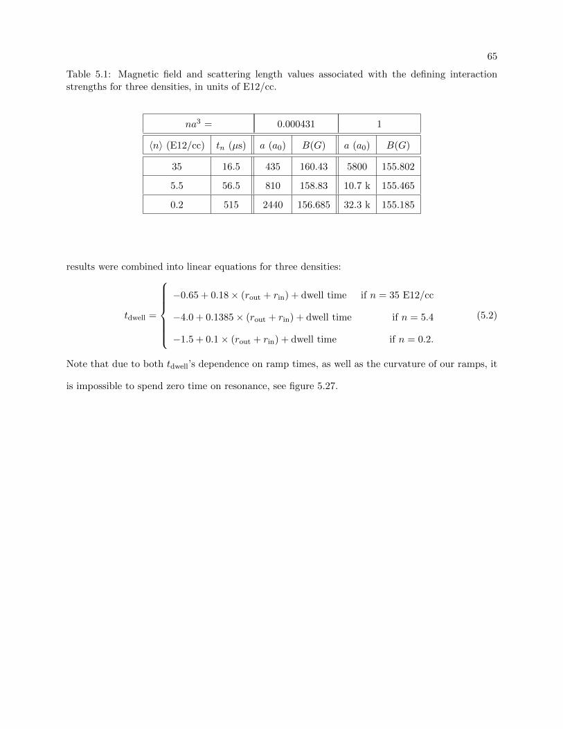
65

Table 5.1: Magnetic field and scattering length values associated with the defining interactionstrengths for three densities, in units of E12/cc.

na3 = 0.000431 1

〈n〉 (E12/cc) tn (µs) a (a0) B(G) a (a0) B(G)

35 16.5 435 160.43 5800 155.802

5.5 56.5 810 158.83 10.7 k 155.465

0.2 515 2440 156.685 32.3 k 155.185

results were combined into linear equations for three densities:

tdwell =

−0.65 + 0.18× (rout + rin) + dwell time if n = 35 E12/cc

−4.0 + 0.1385× (rout + rin) + dwell time if n = 5.4

−1.5 + 0.1× (rout + rin) + dwell time if n = 0.2.

(5.2)

Note that due to both tdwell’s dependence on ramp times, as well as the curvature of our ramps, it

is impossible to spend zero time on resonance, see figure 5.27.

66

20 25 30 35154.5

155.0

155.5

156.0

B (G

)

time ( s)

dwell time = 7us

na3 = 1 for 5.4E12/cc

Figure 5.4: Due to both tdwell’s dependence on ramp times, as well as the curvature of our ramps,it is impossible to spend zero time on resonance. In the plot above, dwell time = 0 and both therin and rout = 25 µs, yet a standard density condensate would still spend 7 µs in the resonanceregime (where na3 > 1 for a standard density of 5.4E12/cc). This 7 µs is 12.5% of the standarddensity’s characteristic evolution time, tn.

5.3 Ramping in

As we have covered, our Fast-B coils and eddy current correction allow us to jump our

cloud to resonance very quickly, in 5 µs. We believe this speed is necessary because the increased

interaction strengths associated with a slow ramp to resonance may result in significant condensate

loss. However, while we believe 5 µs to be “infinitely fast”, as in so fast that the atoms act as if

they were projected onto untarity, we have not yet proven this. We therefore set out to test the

effects of various rin rates. When the rin rate is not infinitely fast, cloud characteristics such as the

number and size will develop a dependence on the rin rate.

67

We ramped a low density condensate to unitarity with various rin rates while correcting the

dwell time such that tdwell = 0.5 tn ≈ 250 µs. The results of such an experiment are shown in figure

5.5. Even for our slowest rin rates of 1500 µs (∼ 3tn) there was very little change in our cloud; we

could not make rin slower due to coil heating limitations. The lack of loss is surprising, as 1500

µs does not seem “infinitely fast”. However, it is comforting that there is no size or number loss

dependence on the rin rate for the shortest times and therefore no reason to believe that a 10 µs

rin is not infinitely fast. We keep rin at 5 or 10 µs for most experiments in this thesis as the fast-B

coils have a finite amount of time they can be on without heating the system, and therefore a fast

ramp-in time allows for more time to evolve at or ramp away from resonance.

In a later experiment where both atoms and molecules were imaged after fast (10 µs) and

slow (250 µs) rin rates we again saw ramp-in independence, see figure 5.6. This experiment further

confirms that there is no rin dependence.

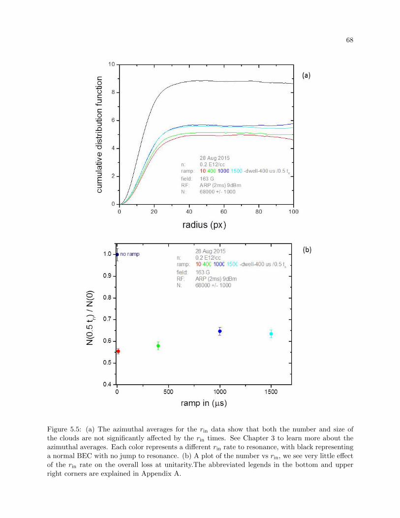
68

Figure 5.5: (a) The azimuthal averages for the rin data show that both the number and size ofthe clouds are not significantly affected by the rin times. See Chapter 3 to learn more about theazimuthal averages. Each color represents a different rin rate to resonance, with black representinga normal BEC with no jump to resonance. (b) A plot of the number vs rin, we see very little effectof the rin rate on the overall loss at unitarity.The abbreviated legends in the bottom and upperright corners are explained in Appendix A.

69

Figure 5.6: (a) The number of atoms as a function of dwell time for both a fast rin (red circles)and a slow rin (blue squares). We see no significant difference between the two datasets. (b) Thenumber of molecules as a function of dwell time for both a fast rin (red circles) and a slow rin (bluesquares). We see no significant difference between the two datasets. The density in both (a) and(b) is 0.2 E12/cc, which has a corresponding evolution time of tn = 510 µs.

70

5.4 Evolving at unitarity

Knowing that we can project a condensate onto resonance infinitely fast, we are free to ponder

the next logical, yet much more exciting question: what happens to a BEC at resonance? To best

answer this question, it is ideal to image resonant BEC while it is on resonance, in action!

Imaging on resonance has many difficulties: (1) the cloud is evolving quickly, in both size

and number; this means that a long imaging pulse, such as the 2ms ARP we employ when imaging

off of resonance, would blur the information together and essentially be too slow to catch the fast

dynamics. (2) While at unitarity the cloud is in trap and we cannot expand it, therefore it is very

small, meaning that is only about 30 µm across. Though we improved our imaging resolution down

to 2.2 µm, we are still unable to trust measurements when optical densities are greater than 15, as

beyond this depth our diffraction-limited resolution worsens. For our typical BEC of 70k atoms, we

expect optical depths of up to 20 when in-trap. (3) Noise in our magnetic field, while small enough

that our atoms remain in the resonance regime, translate into RF noise that distorts imaging. Our

magnetic fields vary at both fast times (due to ringing faster than our servo bandwidth) and slow

times (due to thermal drifts and our cloud falling through a slight vertical magnetic gradient).

In our first attempt to overcome these difficulties we used a 6 µs square microwave pulse to

transfer the atoms from the |2,−2〉 science state to the |3,−3〉 imaging state (once in the imaging

state, the atoms are no longer under resonant interactions and imaging can proceed as normal). At

6 µs, this microwave pulse is faster than the characteristic evolution time at unitarity, tn, which for

our standard density of 5 E12/cc is about 50 µs. We set the pulse power to 5 dBm, this transfers

about 70% of the atoms, keeping the maximum optical depth of the cloud below 15, see figure 5.7.

Unfortunately, the 6 µs pulse is narrow in frequency space, about 25 kHz, and this risks

translating the magnetic field noise into number noise. We account for small drifts in magnetic

field by measuring the microwave center for various dwell times, however we cannot account for

the magnetic field varying more than 25 kHz in 6 µs. A variation on this order would make our

atoms invisible to the microwave during transfer, thereby artificially lowering the measured number.

71

Unfortunately, our magnetic field at short dwell times was found to vary up to 80 kHz in a 6 µs

time span (ignoring the initial 5 µs dwell measurement which varies several MHz, see figure 5.8 and

table 5.2. This variation resulted in artificial lower number at short times, as evident in figure 5.9,

we also found an artificial drop in size at short times due to the microwave noise.

By shortening our microwave pulse to 3 µs we can effectively double the frequency width to

about 50 kHz. This results in substantial improvement in the cloud size measurements at short

time, see figure 5.11. However, shortening the pulse length reduces the number of atoms transferred

to the imaging state if the power is not adequately increased. We are able to send less than 30% of

the atoms to the imaging state with a 3 µs 12 dBm pulse; beyond 12 dBm out microwave amplifier

output saturates. As we had only a 10 watt amplifier in place, we tried placing a 16 watt amplifier

to gain more power, but saw little to no improvement, see figure 5.12. Because our coil’s reflectance

at 2.6 GHz is -7.2 dB (not great), we determined that trying an even larger amplifier would not

yield significantly larger power. We therefore settled for less than 30% transfer fraction. While

this approach has low signal to noise, it is beneficial that the low optical depth never pushes our

imaging resolution, regardless of cloud density, see figure 5.10.

dwell time (µs) dB/dt (mG/µs) ∆f (6µs)

5 534 7.7 MHz

10 5.8 83 kHz

20 2.0 30 kHz

40 >-1 -15 kHz

50 >1 15 kHz

80 0.7 10 kHz

Table 5.2: The variation in magnetic field and in microwave frequency as a function of dwell timeat unitarity. The third column is the variation in peak microwave frequency over ± 3µs centeredat the dwell time.

72

Figure 5.7: (a) The peak optical depth (OD) of a standard density cloud as a function of microwavepower used to transfer the atoms from the science state, |2,−2〉, to the imaging state, |3,−3〉. Weonly trust our imaging system up to an OD of 15, therefore we set the microwave power to 5 dBm.(b) The BEC number as a function of the microwave power. The flat black line represents thetrusted (expected) BEC number, measured with a 9 dBm, 2 ms ARP. We see that with a 5 dBm,6 µs microwave pulse only 70% of the atoms are transferred to the imaging state.

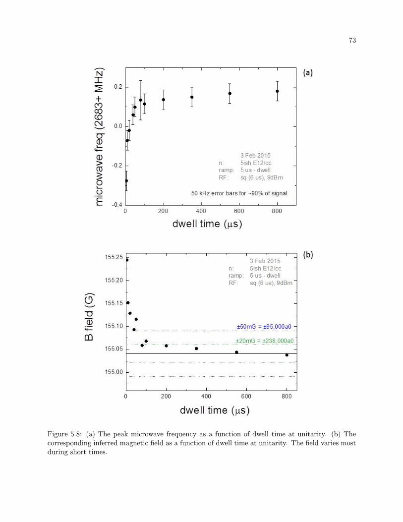
73

Figure 5.8: (a) The peak microwave frequency as a function of dwell time at unitarity. (b) Thecorresponding inferred magnetic field as a function of dwell time at unitarity. The field varies mostduring short times.

74

0 200 400 600 8000.0

0.2

0.4

0.6

0.8

1.0 6 us microwave pulse ARP

atom

num

ber

dwell time ( s)

Figure 5.9: The number of atoms transferred to the imaging state via a 6 µs square microwavepulse on resonance (black circles) or a 2 ms ARP after a 5 µs ramp back to weak interactions(open green triangles) as a function of dwell time. We trust that the ARP transfers all of thesurviving atoms to the imaging state, yet the ramp back to weak interactions may itself lose atoms.The ARP number is therefore a minimum number expectation. Because the on-resonance 6 µsmicrowave pulse transfers less atoms at short dwell times, we conclude that this imaging methodis compromised by field noise.

75

Figure 5.10: (a) The peak optical depth (OD) of a standard density cloud as a function of microwavepower used to transfer the atoms from the science state, |2,−2〉, to the imaging state, |3,−3〉.Because the maximum OD is no greater than 6, we trust the number data for all microwavepowers. (b) The BEC number as a function of the microwave power. We see that with a 12 dBm,3 µs microwave pulse, less than 30% of the atoms are transferred to the imaging state.

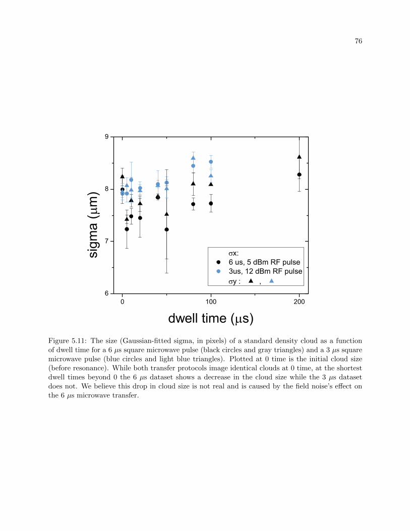
76

0 100 2006

7

8

9

x: 6 us, 5 dBm RF pulse 3us, 12 dBm RF pulse

y : ,

sigm

a (

m)

dwell time ( s)Figure 5.11: The size (Gaussian-fitted sigma, in pixels) of a standard density cloud as a functionof dwell time for a 6 µs square microwave pulse (black circles and gray triangles) and a 3 µs squaremicrowave pulse (blue circles and light blue triangles). Plotted at 0 time is the initial cloud size(before resonance). While both transfer protocols image identical clouds at 0 time, at the shortestdwell times beyond 0 the 6 µs dataset shows a decrease in the cloud size while the 3 µs datasetdoes not. We believe this drop in cloud size is not real and is caused by the field noise’s effect onthe 6 µs microwave transfer.

77

-10 0 10 20

25

30

35

40

microwave power input (dBm)

ampl

ifier

out

put (

dBm

)

10W amplifier 16W amplifier

Figure 5.12: The measured power output from the microwave amplifier as a function of the mi-crowave power input. Around 12 dBm (microwave power input), we see the output of our original10 watt amplifier saturate. While there is a small improvement in power output from the 16 wattamplifier, we ultimately decided to forgo permanent installation.

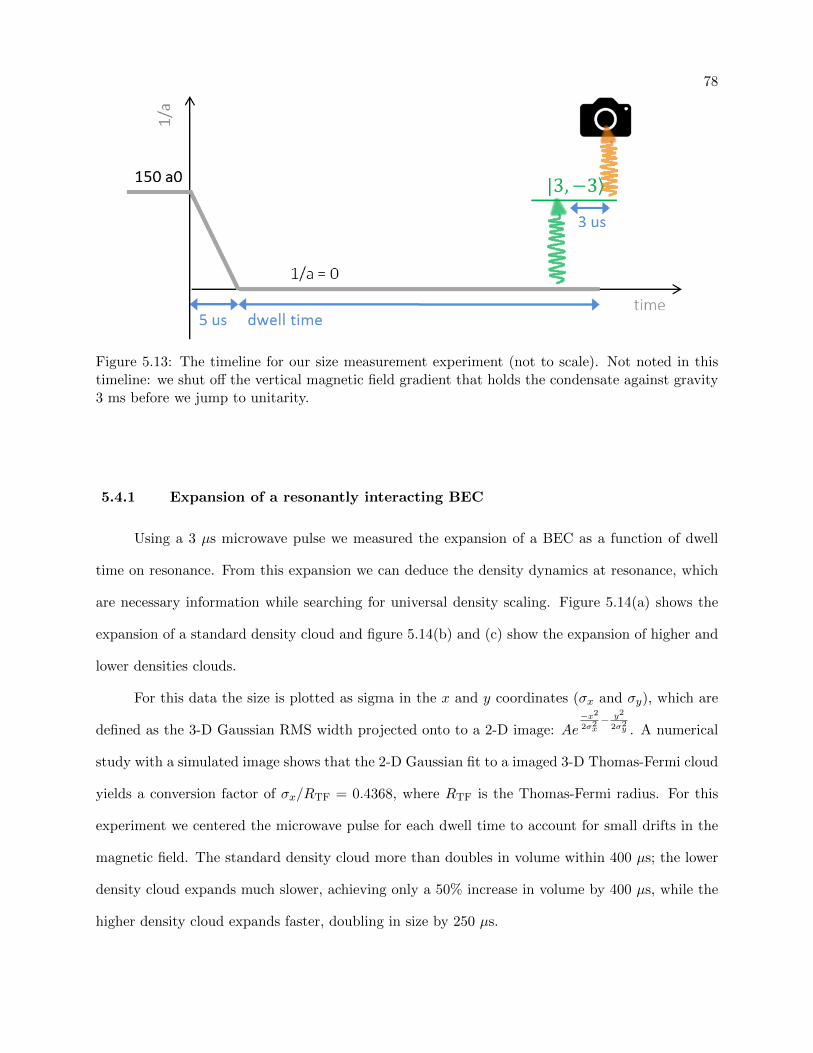
78

Figure 5.13: The timeline for our size measurement experiment (not to scale). Not noted in thistimeline: we shut off the vertical magnetic field gradient that holds the condensate against gravity3 ms before we jump to unitarity.

5.4.1 Expansion of a resonantly interacting BEC

Using a 3 µs microwave pulse we measured the expansion of a BEC as a function of dwell

time on resonance. From this expansion we can deduce the density dynamics at resonance, which

are necessary information while searching for universal density scaling. Figure 5.14(a) shows the

expansion of a standard density cloud and figure 5.14(b) and (c) show the expansion of higher and

lower densities clouds.

For this data the size is plotted as sigma in the x and y coordinates (σx and σy), which are

defined as the 3-D Gaussian RMS width projected onto to a 2-D image: Ae−x2

2σ2x− y2

2σ2y . A numerical

study with a simulated image shows that the 2-D Gaussian fit to a imaged 3-D Thomas-Fermi cloud

yields a conversion factor of σx/RTF = 0.4368, where RTF is the Thomas-Fermi radius. For this

experiment we centered the microwave pulse for each dwell time to account for small drifts in the

magnetic field. The standard density cloud more than doubles in volume within 400 µs; the lower

density cloud expands much slower, achieving only a 50% increase in volume by 400 µs, while the

higher density cloud expands faster, doubling in size by 250 µs.

79

Figure 5.14: (a) Expansion data for a condensate of standard initial density. Sigma is the gaussianfitted cloud width in pixels, with a 1.1 px resolution correction. The atoms were transferred fromthe resonantly interacting science state to the imaging state using a 3 µs 9 dBm square microwavepulse. We see that the cloud grows, but this growth slows around 400 µs unexpectedly. (b)Expansion data at a lower density of 1.1 E12/cc, with a 1.1 px resolution correction. (c) Expansiondata at a higher density of 12.1 E12/cc, with a 1.1 px resolution correction.

After substantial expansion at unitarity however, the clouds are no longer well described by

a Gaussian fit [see figure 5.15(b)]. Attempting to fit the clouds with a Gaussian fit yields erroneous

results for two reasons : (1) the expanded cloud is no longer well-described by a 3-D Thomas-Fermi

distribution because the center of the cloud loses density faster than the edges of the cloud, and

80

(2) a bump in the optical depth (at 30 microns) could cause a Gaussian to fit artificially larger;

this bump is present in our images of non-resonant condensates, we therefore conclude it is not an

artifact from resonance.

This bump at 15 pixels is not real, it is an artifact of diffraction. By imaging clouds of various

condensate fractions (see figure 5.16) we determined that this bump is not a halo of thermal atoms.

We varied the condensate fraction, or percentage of atoms in a cold condensed form as opposed to a

hotter thermal gas, by varying the frequency of the RF knife used to spin-flip the hot atoms during

our final stage of evaporation. For example, an RF knife of 81.78 MHz yields a condensate fraction

of only 20%, whereas any knife of 81.725 MHz or below yields a pure condensate. The bump

becomes less pronounced when imaging a condensate surrounded by a large thermal component

and more pronounced when imaging a more pure BEC, this result confirms out hypothesis that the

bump is a result of diffraction. Further confirmation was had after reducing the amount of incident

light on the atoms and seeing the bump become less pronounced, see figure 5.17.

Because the Gaussian approximation is unfit to describe a resonant condensate, we instead

use the full-width-half-max (FWHM) of the optical density (OD), defining FWHM as the radius

at which the OD has dropped to half its peak value. In the case of a Thomas-Fermi distribution,

RTF =√

2FWHM and σi = 0.618 FWHMi. With this new size definition the standard density

cloud now expands by less than 50% its initial volume by 400 µs, see figure 5.18.

We return now to our goal of determining the density dynamics of a resonant condensate by

combining the expansion of the cloud with the number loss. While we can measure the condensate

number with the 3 µs on-resonance transfer pulse, the small signal to noise (due to only trans-

ferring less than 30% of the atoms to the imaging state) is undesirable. These measurements are

also difficult because each dwell time requires an individual line shape, and the process of taking

these lineshapes can take hours, over which the magnetic fields experience small thermal drifts,

introducing more noise. For these reasons we opt instead to ramp away to a weaker scattering

length before imaging the cloud with a long ARP’d pulse that gaurantees 100% transfer.

81

Figure 5.15: (a) The azimuthal averages for the standard density expansion data. The data wereazimuthally averaged before clouds with common dwell times were averaged together. The moststriking characteristic that evolves with dwell time is the drop in peak optical density. The insetzooms in on the bump that occurs in all datasets around 15 pixels (px = 1.996 µm) (b) Theazimuthal averages scaled by their peak optical depth. This scaling emphasizes how the tail atlarge radii grows over time, causing the cloud to deviate from a typical Gaussian shape .

82

20 40 600.00

0.25

0.50

0.75Imaging Pulse 3us, 9dBm

optic

al d

epth

radius ( m)

RF = 81 MHz + 705 710 715 720 723 725

(out of BEC) 728 730 740 750 770 780 kHz

20 March 2015

Figure 5.16: The cumulative distribution functions of clouds with various condensate percentages.For the least-invasive RF knives, such as the black curve, the cloud is almost 80% thermal atomsand only 20% cold condensate. These larger, hotter clouds wash away the bump at 15 pixels. Forthe nearly 100% condensates, i.e. any curve that has an RF knife of 81.725 MHz and below, thebump becomes pronounced. The bump only begins to shrink again for the closest RF knives, suchas 81.710 and 81.705 MHz, yet this corresponds with an overall drop in peak optical depth, seeinset. This bump behavior is consistent with diffraction around the condensate.

83

Figure 5.17: The azimuthal average of a pure condensate for various intensities of incident light.In order to properly image our high optical density condensate, we employ high-intensity imagingtechniques (see Chapter 3) that involve using about 50 times more incident light than normalabsorption imaging. This increase in light increases the amount of light diffracted around thecondensate, thereby increasing the size of the artificial diffraction bump. We see that by loweringthe intensity of the light we are able to minimize this bump. However, the lower light intensitiesare unable to fully image the large optical depths of our condensate, resulting in artificially lowpeak optical depths, see inset.

84

0 200 400 600 8008

10

12

14

17 March 2015n: 5.75 E12/ccramp: 5-dwell-5 usfield: 155.04 GRF: sq (3 us)

9 dBm, N/A, no N: 69600 +/- 2400

x y FWHM

size

(m

)

dwell time ( s)Figure 5.18: The expansion of a standard density condensate as a function of dwell time at res-onance. The red squares are the size as described by FWHM, and the black points and opentriangles are x and y sizes described by the Gaussian RMS width, σ. For a perfect Thomas-Fermidistribution, σ should be 0.618× FWHM, however σ at all times appears to be greater than thisvalue, this is most likely due to artificial expansion due to fitting a cloud with a bump at 15 pixels.At later times, σ becomes almost the same value as FWHM, most likely because of the non-gaussianexpansion of the cloud. We opt instead to use the FWHM to describe the size our cloud.

85

Figure 5.19: The timeline for our number measurement experiment (not to scale). We ramp awayfast (in 5 µs) from resonance to weak interactions, then expand the cloud at 500 a0 for 20 ms tolower the peak optical depth of the cloud for imaging. Because field gradients do not affect ARPtransfers, we do not turn off the vertical magnetic gradient in this procedure.

5.4.2 Ramping away before imaging

Ramping away from resonance very quickly before imaging with a long, 2 ms adiabatic rapid

passage (ARP) transfer to the imaging state yields almost the same number as our on-resonance

3 µs RF pulse method, see figure 5.20. While the ARP method allows us to obtain data much

faster (because a line shape for each dwell time is no longer necessary) it does lose size and shape

information about the cloud, and is therefore only useful for obtaining number data.

Combining the ramped-away ARP number data with on-resonance short-pulse size data we

obtain the density as a function of dwell time at unitarity, see figure 5.21. The density initially

drops off very quickly, falling to 85% in 50 µs (∼ 1 tn) and 61% in 100 µs (∼ 2 tn). The number

loss is the main cause of the drop in density, accounting for about 70% at both the shortest and

longest dwell time measurements.

The significant change in density of the cloud while at resonance makes searching for density

86

0 200 400 600 8000

20k

40k

60k

80k

100k

23 March 2015n: 5ish E12/ccramp: 5-dwell-5 usfield: 155G 163 GRF: sq (3 us)

ARP (2ms)9 dBm, N/A, no

aver

age

Num

ber

dwell time ( s)Figure 5.20: The number of atoms as a function of dwell time on resonance after imaging on-resonance with a 3 µs square RF pulse (green points) or ramping away to weak interactions in 5µs, expanding at 500 a0 for 20 ms, and then imaging with a 2 ms ARP (black points). We concludethat the latter measurement technique results in similar number with reduced noise. And mostimportant to a graduate student, data taken with the latter technique is much faster to procure,meaning more data, happier advisors, and a less stressed student.

dependent universality more challenging. While many experiments exploring Bose gases on reso-

nance are interested in testing the predicted n2/3 dependent loss rates [37, 39, 70, 83], the changing

densities complicate this analysis. As can be seen in figure 5.22, the number over time does not

follow a simple exponential loss rate.

The exponential in figure 5.22 assumes no density dependence in the loss rate, assuming the

three-body loss rate, Γ3, is constant, i.e. assuming the density does not change. This non-density

87

0 200 400 600 8000.0

0.2

0.4

0.6

0.8

1.0 n: 5.75 E12/ccramp: 5-dwell-5 us

Number Data:14 April 2015

field: 163 GRF: ARP (2ms) 9 dBm Size Data:

17 March 2015field: 155.04 GRF: sq (3 us) 9dBm

rela

tive

dens

ity

dwell time ( s)Figure 5.21: The relative density of a standard density condensate as a function of dwell time atdensity. This data was calculated by combining the ARP number data and 3 µs RF size data. Wesee an initial fast drop in density, with the condensate density dropping to 85% in 50 µs and 61%in 100 µs, which correspond to roughly 1 and 2 tn. The point at 0 dwell time corresponds to theinitial density of the cloud (1) before the resonance jump.

dependent loss rate, given in equation (2.15) can be rewritten as

ln

(N(t)

N(0)

)= −Γ3N, (5.3)

and therefore the linear fit in 5.23(a) has a slope of Γ3.

If the density dependence of the loss rate was as simple as n2/3, we could correct for the

changing density while the cloud evolves at unitarity as a test of the loss rates’ density dependence.

To include the n2/3 dependence, Γ3 can be rewritten as L′3 × 〈n2/3〉, where L′3 is the adjusted

three-body loss rate constant and 〈n2/3〉 is the mean density to the two-thirds, =∫n·n2/3 d3r∫n d3r

; for a

88

0 200 400 600 8000

20k

40k

60k

80k

100k

14 April 2015n: 5.75 E12/ccramp: 5-dwell-5 usfield: 163 GRF: ARP (2ms)

9 dBm, N/A, no N: 69700 +/- 1500

number

dwell time ( s)Figure 5.22: The number of atoms in our standard density condensate as a function of dwell timeat resonance. We see a poor fit to the exponential, this is due to the changing density of the cloudwhile it evolves at unitarity.

Thomas-Fermi distribution, 〈n2/3〉 = 0.259〈n〉. We can then rewrite

N = L3 × 〈n2/3〉N (5.4)

as

ln

(N(t)

N(0)

)= −C · L3

∫ t

0

(N(t′)

w(t′)3

)2/3

dt′. (5.5)

we now define G(t) as L3

∫ t0

(N(t′)

w(t′)3

)2/3dt′ and plot the log of the change in number as a function

of G(t) in figure 5.23(b).

We see that an n2/3 dependence does not properly describe the resonant loss. This could be

true for a variety of reasons, such as the loss rate has a universal scaling other than n2/3, there is

89

a nearby Efimov state that is perturbing this loss, but most likely we are losing vital information

by defining our cloud size by the optical depth FWHM. Essentially, we have assumed that the

actual density, n(r), can be approximated by n ∝ N(t)FWHM(t)3 . But the actual density of the cloud

varies from npk to 0 across the radius of the cloud, and if the loss rate goes locally as n2/3, there

will be more number loss in the center of the cloud than at the edges. This could change the

function of n(r), and therefore the local decay could goes as n(r)2/3, but this would not be equal to(N

FWHM3

)2/3loss. If this were the case, the decay in terms of

(N

FWHM3

)xwould still be the same

for different initial densities.

Being unable to extract the density dependence of the loss rate by examining the loss as a

function of dwell time, we instead look at the loss at short times where the change in density is

still small and the expansion nearly negligible. If we examine four datasets, with initial densities

spanning from 1.1 to 12.5 E12/cc, we see that the short time loss roughly agrees with n2/3 scaling,

see figure 5.24.

90

Figure 5.23: (a) The same data from figure 5.22, now plotted as the log of the number of atoms inour standard density condensate as a function of dwell time at resonance as the natural log of thechange in number. In this plot, a perfect exponential decay would appear as a straight line. Wecan see that the data has a poor fit to the exponential decay as it deviates from the fitted straightline. (b) The same data as in (a), however the x-axis is now the function G(t), given by equation5.5. In this plot, a perfect exponential decay that accounts for an n2/3 dependence would follow astraight line. We see that while this data follows a straight line better than that in (a), it is farfrom perfect. We conclude from this that we do not see n2/3 density dependence in the loss rate asa function of dwell time on resonance.

91

0 1 2 3 40.0

0.2

0.4

0.6

0.8

1.0

22 April 20151.1 E12/cc18 May 20153.1 E12.cc17 March 20155.75 E12/cc19 May 201512.5 E12/cc

ramp: 5-dwell-5 usfield: 155.04 GRF: sq (3 us) 9 dBm

N/N

(0)

tdwell / tn

Figure 5.24: The relative change in number vs tdwell, scaled by the density-dependent units oftn. The four initial densities seem to have the same loss rate in units of tn, hinting at an n2/3

dependence in the loss rate.

92

5.4.3 Atom loss at Unitarity

The next experiment involves ramping to resonance in 5 µs, dwelling on resonance for 1 tn,

then ramping away in 5 µs. We varied the density by over a factor of 250 using techniques outlined

in Chapter 4. The recorded loss is plotted as a function of density in figure 5.25. We see very good

agreement with the n2/3 scaling, however there is some slight deviation from this scaling at the

larger densities, and for a single point at the smallest density. To examine further, we replot this

data as Γ3/n2/3, see figure 5.26. From this replotting we see that this small deviation is actually

quite large and could fit to a log-periodic curve, which is an Efimov smoking gun. If these deviations

in the loss rate were due to the presence of the Efimov states, they would be correcting the loss rate

by more than 50%. In [83] the oscillations in loss rate due to the Efimov effect in a thermal Bose

gas at unitarity were theorized to be 0.022e−2η∗ . For 85Rb, η∗ is 0.057 [34], yielding an expected

amplitude correction of only 2%. In any case, these calculations were for non-degenerate gases in

which T is varied, not a degenerate gas in which n is varied. There is preliminary work by Jose P.

D’Incao which predicts larger oscillations [84].

There are a myriad of ways to kill a BEC, and therefore many other possibilities to explain

this deviation in n2/3 loss rate scaling. It is suspicious that the least loss occurs near our standard

density of 5 E12/cc. While we verified that no loss was occurring during the density expansion /

compression procedures, it is possible that the densities at the far ranges of the spectrum could

be slightly off from their calculated values (see Chapter 4 for more details). An incorrect density

would lead to an incorrect value of tn, and if tn was smaller than calculated, the cloud would

spend a longer time at unitarity. However, for this to explain both the deviations at high and

low densities it would require that our actual densities were always lower than calculated, when

in reality it is more likely that errors in our density calculations would lead to either overshooting

or undershooting the change in density regardless of an expansion or compression. This paranoia

could be disproved by taking loss data across an even larger density range, beyond the predicted

turning point, to confirm that the deviation is log-periodic and not just coincidentally increasing.

93

0.1 1 10

1E-3

0.01

(1/

s)

density (cm-3) /1012

May 2015 Data

Figure 5.25: The measured loss rate, Γ3 = (1−N(t)/N(0)) /1 tn, as a function of initial condensatedensity. The solid blue line represents the predicted universal n2/3 scaling and the red dashed linerepresents the mean-field loss rate n2 scaling. The red points at large n have a density larger than35 E12/cc, the highest verified density, see Chapter 4.

Another controlled variable to scrutinize is the rout rate to weak interactions. In this experi-

ment the rout was always 5 µs. We naively assumed that the number of atoms before and after the

jump were practically the same. However, further investigation reveals that the rout has a larger

effect on the system than one might assume at first glance. Whether the ramp to weak interactions

in this experiment should be consistent in units of rin or tramp in order to probe only the effects of

tdwell was (is still?) hotly debated in our lab.

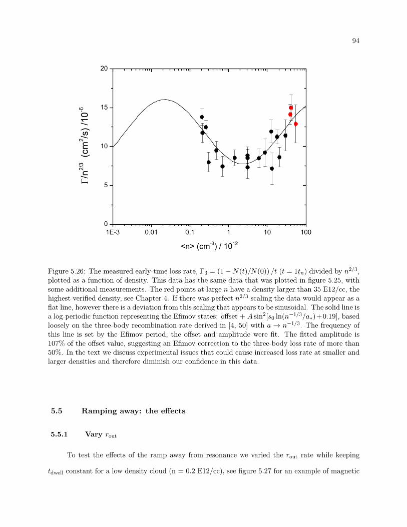
94

1E-3 0.01 0.1 1 10 1000

5

10

15

20

<n> (cm-3) / 1012

/n2/

3 (cm

2 /s) /

10-6

Figure 5.26: The measured early-time loss rate, Γ3 = (1−N(t)/N(0)) /t (t = 1tn) divided by n2/3,plotted as a function of density. This data has the same data that was plotted in figure 5.25, withsome additional measurements. The red points at large n have a density larger than 35 E12/cc, thehighest verified density, see Chapter 4. If there was perfect n2/3 scaling the data would appear as aflat line, however there is a deviation from this scaling that appears to be sinusoidal. The solid line isa log-periodic function representing the Efimov states: offset + A sin2[s0 ln(n−1/3/a∗)+0.19], basedloosely on the three-body recombination rate derived in [4, 50] with a → n−1/3. The frequency ofthis line is set by the Efimov period, the offset and amplitude were fit. The fitted amplitude is107% of the offset value, suggesting an Efimov correction to the three-body loss rate of more than50%. In the text we discuss experimental issues that could cause increased loss rate at smaller andlarger densities and therefore diminish our confidence in this data.

5.5 Ramping away: the effects

5.5.1 Vary rout

To test the effects of the ramp away from resonance we varied the rout rate while keeping

tdwell constant for a low density cloud (n = 0.2 E12/cc), see figure 5.27 for an example of magnetic

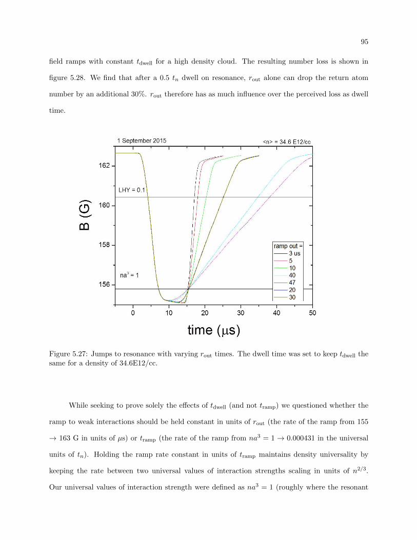
95

field ramps with constant tdwell for a high density cloud. The resulting number loss is shown in

figure 5.28. We find that after a 0.5 tn dwell on resonance, rout alone can drop the return atom

number by an additional 30%. rout therefore has as much influence over the perceived loss as dwell

time.

Figure 5.27: Jumps to resonance with varying rout times. The dwell time was set to keep tdwell thesame for a density of 34.6E12/cc.

While seeking to prove solely the effects of tdwell (and not tramp) we questioned whether the

ramp to weak interactions should be held constant in units of rout (the rate of the ramp from 155

→ 163 G in units of µs) or tramp (the rate of the ramp from na3 = 1 → 0.000431 in the universal

units of tn). Holding the ramp rate constant in units of tramp maintains density universality by

keeping the rate between two universal values of interaction strengths scaling in units of n2/3.

Our universal values of interaction strength were defined as na3 = 1 (roughly where the resonant

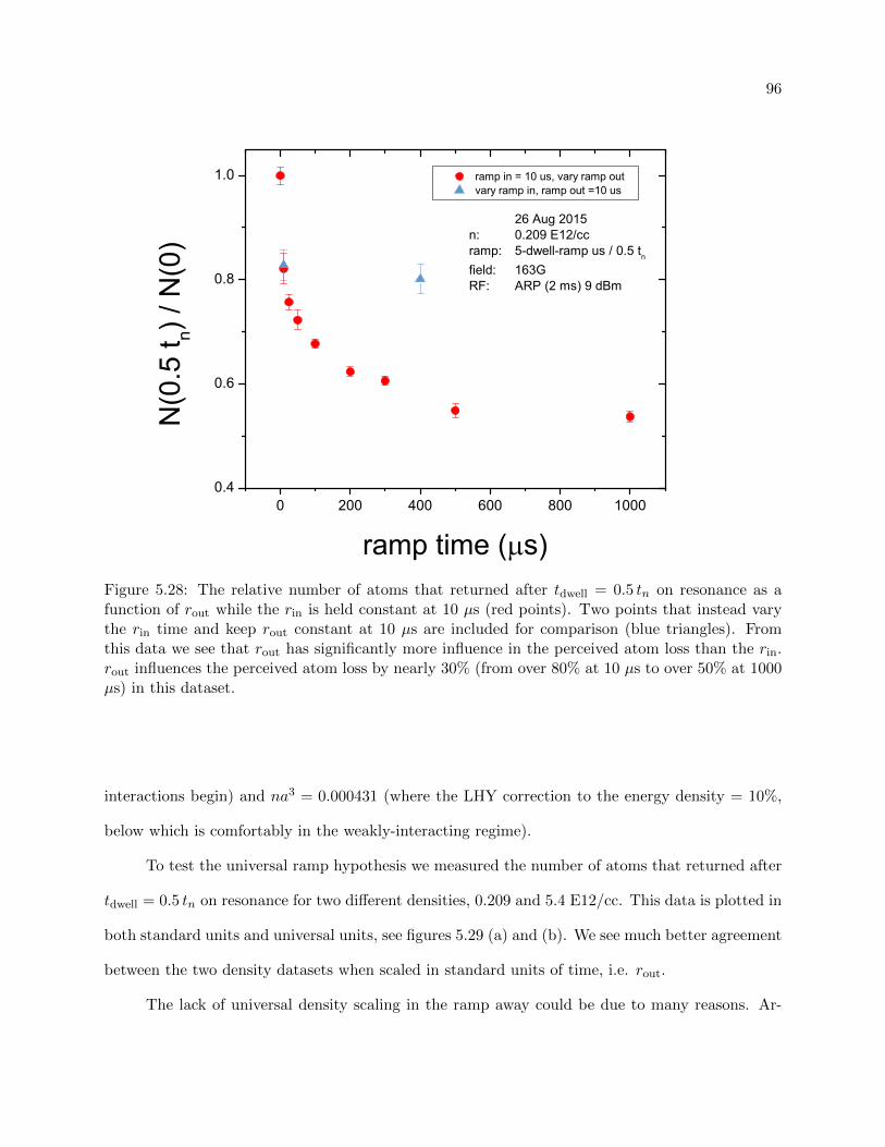
96

0 200 400 600 800 10000.4

0.6

0.8

1.0

26 Aug 2015n: 0.209 E12/ccramp: 5-dwell-ramp us / 0.5 tn

field: 163GRF: ARP (2 ms) 9 dBm

ramp in = 10 us, vary ramp out vary ramp in, ramp out =10 us

N(0

.5 t n)

/ N

(0)

ramp time ( s)Figure 5.28: The relative number of atoms that returned after tdwell = 0.5 tn on resonance as afunction of rout while the rin is held constant at 10 µs (red points). Two points that instead varythe rin time and keep rout constant at 10 µs are included for comparison (blue triangles). Fromthis data we see that rout has significantly more influence in the perceived atom loss than the rin.rout influences the perceived atom loss by nearly 30% (from over 80% at 10 µs to over 50% at 1000µs) in this dataset.

interactions begin) and na3 = 0.000431 (where the LHY correction to the energy density = 10%,

below which is comfortably in the weakly-interacting regime).

To test the universal ramp hypothesis we measured the number of atoms that returned after

tdwell = 0.5 tn on resonance for two different densities, 0.209 and 5.4 E12/cc. This data is plotted in

both standard units and universal units, see figures 5.29 (a) and (b). We see much better agreement

between the two density datasets when scaled in standard units of time, i.e. rout.

The lack of universal density scaling in the ramp away could be due to many reasons. Ar-

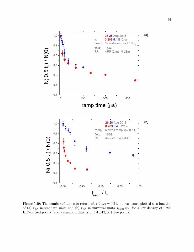
97

Figure 5.29: The number of atoms to return after tdwell = 0.5 tn on resonance plotted as a functionof (a) rout in standard units and (b) rout in universal units, tramp/tn, for a low density of 0.209E12/cc (red points) and a standard density of 5.4 E12/cc (blue points).

98

guably the most important component of the ramp away is the very beginning of the ramp, when

the atoms cross from the resonant to strongly-interacting regime. As discussed earlier, our ramp is

a piece-wise function with curved edges. The first 12.5% of the ramp (1 Gauss of the total 8 in this

case) is in the non-linear regime, and this is also where the critical crossing out of the resonantly

interacting regime occurs for all densities. It is possible that the non-linear ramp at na3 = 1 is the

cause of our ramp’s non-universal behavior. So we instead rethought the problem and found a way

to test it:

We know that the ramp up to and beyond na3 > 1 is non-linear and therefore not well

characterized by our theory. rout to na3 = 0.000431 is linear for all densities. Our universal ramp-

away theory assumes that the ramp rate between only 1 ≤ na3 ≤ 0.000431 determines the atom

loss. If this were true, a two-component ramp that was at first “slow” and then for na3 < 0.000431

“fast” should produce the same loss as an entirely “slow” ramp. The results of such an experiment

are shown in figure 5.30.

The two-component ramp loss not only disagrees with the single-component “slow” ramp

loss, its disagreement seems to vary with the dwell on resonance, which is very unexpected. For

example, the two-component ramp seems to yield identical results to the slow ramp at the shortest

dwell time of tdwell = 84 µs, however beyond this dwell time the two-component ramp proceeds to

match the linear decay of the fast ramp while the fast ramp has a non-linear loss that accelerates

and then stabilizes. This suggests that there is more happening at unitarity than simple loss to

deeply bound states.

99

Figure 5.30: (a) There are three ramps in this experiment: two were single-component rampscharacterized as 10 µs“fast ramp” (blue) and a 400 µs “slow ramp” (black) and the third ramp wasa two-component ramp (red) that matched the “slow” ramp for na3 ≥ 0.000431 and the fast rampfor na3 < 0.000431. The inset shows this two-component ramp on a linear scale. (b) The numberof atoms that returned as a function of dwell time for each respective ramp.

100

5.5.2 Understanding the loss

Understanding the loss associated with the ramp away requires a shift in our patterned

thinking. Suspicious that the increase loss associated with slower ramps away from resonance was

caused by Fesbach molecule production (atoms in a superposition of unbound and bound molecule

states have previously been observed in a similar system after pulsing to large a, see [85]), we

theorized that we could sweep these molecules back into atoms. If we then jumped back to weak

interactions quickly, we could image the return of the missing atoms, see figure 5.31 for the magnetic

ramps. In figure 5.32 we see that such an experiment resulted in nearly all the atoms returning,

with the exception of the the farthest magnetic ramp (we attribute the increased loss in this point

to finite Feshbach molecule lifetime).

Having confirmed the creation of Feshbach molecules, further investigation requires another

shift in patterned thinking: we should image the molecules directly.

101

0 250 500 750 1000

156

158

160

162

B (G

)

time ( s)

single ramp: 10 s ramp out 500 s ramp out

ramp there and back:B mid value =

156.685 (LHY = 0.1) 158.2 159.8 162.9 G (B0)

Figure 5.31: There were two single-component ramps used as reference points for this experiment:a fast 10 µs ramp (gray) and a slow 500 µs ramp (magenta). Four ramps ramped away first at theslow ramp rate to various values of magnetic field before ramping back in at the same rate; theylater jumped back (at the fast ramp rate) to the initial magnetic field for imaging. The total dwelltime on resonance was around tdwell = 0.5 tn (for a n = 0.2 E12/cc cloud) and was split betweenthe first and second time at resonance for the double ramps; the measured values of tdwell were 255,249, 268, 260, 266, and 240 µs for the ramps in the order of the legend, respectively.

102

0.00 156 158 160 162 164

0.6

0.8

1.0

2 Sept 2015n: 0.2 E12/ccramp: 10-dwell-500-0-500-dwell-10 us / 0.5 tnfield: 163 GRF: ARP (2ms)

9dBm, N/A , no N: 54700 +/- 1200

N(0

.5 t n)

/ N

(0)

Bmid (G)

10 us ramp out

500 us ramp out

no jump

Figure 5.32: The number of atoms measured after the final jump back to the initial magnetic fieldfor the ramps shown in figure 5.31. By ramping back to resonance slowly and then jumping outquickly we were able to see a return of almost all of the atoms , with the exception of the cyanpoint which ramped all the way back to the initial magnetic field - while it certainly had more finalatoms than if we had only just ramped away slowly, not all of the atoms were able to return. Weattribute this loss to loss of the molecules due to finite molecule lifetime at our initial magneticfield.

Chapter 6

Dissociating molecules for imaging

To image molecules directly, we use a microwave pulse to simultaneously dissociate the

molecule and spin-flip one of the molecular atoms from the |2,−2〉 science state to the |3,−3〉

imaging state. In this chapter we will discuss the relevant binding energy of the molecules as well

the three microwave pulses we can use to spin flip molecules into the imaging state.

6.1 Molecular binding energy

6.1.1 Theory

A simple analytic formula for the excitation rates and lineshapes of the molecular dissociation

spectra was derived based on the scattering theory in the threshold regime in [86]. Because our

imaging state has a negative scattering length of a′ ≈ −500 a0, the pulse excites a bound-free

transition that results in molecule dissociation. In this event only one atom in the molecule is

excited to the imaging state. The minimum energy required for this pulse (Erf) is equal to the

|2,−2〉 → |3,−3〉 energy difference E0 (around 2.6 GHz for our conditions) plus the additional

binding energy of the molecule Eb, typically on the order of 100 kHz, but molecules can also be

dissociated in this manner with microwave pulses of greater energy. The peak of the dissociation

spectra occurs with an additional (1/3)Eb, or Erf = E0 +(4/3)Eb. The dissociation effectiveness of

the microwave pulse is related to many factors, including the intensity and the duration of the pulse,

however we will focus mainly on the detuning of the microwave pulse from the atom resonance, δ.

104

Figure 6.1: The energy diagram of 85Rb at 159.5 G. Our atoms begin in the science state |2,−2〉,the Feshbach molecules are bound by 110 kHz. Our imaging state, |3,−3〉, is 2.674 GHz away fromthe science state when B = 159.5G. We can transfer molecules to the imaging state by applyingan RF with a frequency greater than 110 kHz + 2.674 GHz.

In the small Rabi frequency limit, the bound-free transition rate is given by

Γf (K) =hΩ2

2Ff (K), (6.1)

where Ω is the rf Rabi frequency and Ff (K) is the bound-free Franck-Condon factor per unit

energy, and K is the kinetic energy of the outgoing wave with wave number k, K = ~2k2/m. The

Franck-Condon lineshape is derived in [86] to be

Ff (K) =2

π

(1− a′

a

)2 K1/2E1/2b E′b

(K + Eb)2(K + E′b)2, (6.2)

where E′b ≡k2a′2

K , and a′ is the scattering length of our imaging state. Defining the microwave

105

offset energy as E ≡ Erf − E0 = K + Eb, we can rewrite equation (6.2) as

Ff (E) =2

π

(1− a′

a

)2 E′bE1/2b (E − Eb)1/2

E2 (E + E′b + Eb). (6.3)

We have plotted these lineshape as a function of microwave detuning (δ = E/h) from the atomic

resonance, E0, for initial scattering lengths of a = 1000, 700, and 500 a0 in figure 6.2. We observed

the molecular lineshape with microwave spectroscopy and saw good agreement with this theory,

see figure 6.3.

Figure 6.2: The Franck-Condon factor as a function of microwave detuning from the atomiclineshape for initial scattering lengths of a = 1000 (green), 700 (orange) and 500 (blue) a0 toa′ ≈ −500 a0 represents the the bound-free dissociation spectra of our Feshbach molecules. Thebinding energies of the molecules at these scattering lengths are 50, 110, and 240 kHz respectively.As is shown in this figure, molecules can be dissociated by microwave pulses with energies equal toor greater than their binding energies, and the peak of the dissociation rate occurs at (4/3)Eb.

Due to their close proximity, the bound molecular atoms have large uncertainty in momentum.

This momentum is released during dissociation, thereby causing them to fly apart. For this reason,

our molecular atoms are not at risk for reassociating into molecules with continued microwave

exposure. Therefore we can dissociate all of the molecules with a long microwave pulse without

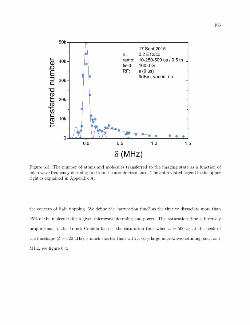
106

0.0 0.5 1.0 1.50

10k

20k

30k

40k

50k17 Sept 2015

n: 0.2 E12/ccramp: 10-250-500 us / 0.5 tnfield: 160.0 GRF: s (9 us)

9dBm, varied, no

trans

ferr

ed n

umbe

r

(MHz)Figure 6.3: The number of atoms and molecules transferred to the imaging state as a function ofmicrowave frequency detuning (δ) from the atomic resonance. The abbreviated legend in the upperright is explained in Appendix A.

the concern of Rabi flopping. We define the “saturation time” as the time to dissociate more than

95% of the molecules for a given microwave detuning and power. This saturation time is inversely

proportional to the Franck-Condon factor: the saturation time when a = 500 a0 at the peak of

the lineshape (δ = 320 kHz) is much shorter than with a very large microwave detuning, such as 1

MHz, see figure 6.4.

107

0 50 100 150 2000

2k

4k

6k

31 March 2016n: 5.5 E12/ccramp: 10-108-100 us / 2.0 tnfield: 160.0 / 507 a0RF: s (50 us)

9dBm, varied, no N: 79800 +/- --

0.35MHz detuning 1.1MHz detuning

num

ber

microwave pulse duration ( s)

Figure 6.4: The number of molecules measured as a function of microwave pulse duration for twomicrowave detunings : δ = 350 kHz (pink squares) and 1.1 MHz (blue points). The former isclose to the peak of the molecular lineshape while the latter is far away, therefore we expect theformer to saturate faster. And indeed, we see the δ = 350 kHz data saturate in about 50 µs, andthe δ = 1.1 MHz data saturate after 150 µs. These numbers are not equal, possibly because themolecular atoms dissociated by the large detuned pulse fly apart with much more energy.

6.1.2 Experimental considerations

Because the dissociation rate of the molecules depends on the detuning from the atomic

resonance, and the exact frequency of the atomic resonance is sensitive to the magnetic field, the

dissociation of the molecules could be sensitive to magnetic field noise. However, as long as our

microwave pulse is equal to or longer than the saturation time, small changes in the magnetic field

will not translate into number noise.

Because in the future we will probe temporal molecular dynamics, we wish to keep the

108

microwave pulse length constant and greater than the saturation time. We therefore find that we

need to adjust the microwave detuning as we vary the scattering length a at which we probe the

molecules. By changing the microwave detuning such that the Franck-Condon remains the same,

we find that the saturation time does not vary. For example, a microwave detuning of 400 kHz at

500 a0 has the same Franck-Condon as 315 kHz at 700 a0 and 214 kHz at 1000 a0 (see figure 6.5)

therefore the saturation times at these detunings are also equal (assuming constant intensity of the

microwave pulse), and are about 50 µs, see figure 6.6.

Figure 6.5: A curve representing a contour of constant Franck-Condon factor for detuning from theatom resonance as a function of scattering length. We see that 400 kHz detuning at 500 a0 spinflips as many molecular atoms as a 315 kHz detuning at 700 a0 and 214 kHz at 1000 a0.

Because a 50 µs square pulse is very narrow in frequency space (relatively speaking in com-

parison to the other energy scales), it is necessary to turn off the vertical magnetic gradient that

holds the atoms up against the gravity . The cloud then falls for a few ms during the experiment,

109

0 50 100 150 2000

2k

4k

6k

8k

500 a0, 400 kHz detuned 700 a0, 302 kHz detuned

9dBm square pulse

num

ber

microwave pulse duration ( s)

Figure 6.6: The number of molecules as a function of microwave pulse duration for a squaremicrowave pulse at 9 dBm nominal power. The molecules at 500 a0 were probed with 400 kHzdetuning (blue points), the 700 a0 at 302 kHz (orange squares). The saturation times are bothroughly 50 µs, and the total molecule number appears to be about the same.

traveling less than 100 µm, or about three cloud diameters, see figure 6.7.

110

0 2 4 6 8

200

250

300

350

Model: ParabolaEquation: y = A + B*x + C*x^2

A 182.01 ±0.72B 0 ±0C 2.470 ±0.022

y ce

nter

(px)

time since vertical gradient off (ms)

Figure 6.7: The vertical position of the cloud center as a function of time after turning off thevertical magnetic gradient. We see that within 4 ms the cloud falls less than 100 µm. Thereremains a small field gradient despite turning off the applied field gradient. This is evident by theacceleration of the cloud, measured to be just slightly less than gravity’s pull. From this discrepancywe infer a residual field gradient of 1 G/cm in the vertical direction.

6.2 Square RF pulses

6.2.1 Atoms, atoms everywhere

While many atoms are bound into molecules by our ramp away from resonance, the majority

of atoms in our system remain unbound. For the atoms, the 50 µs, 9 dBm square microwave pulse

corresponds to a 6-π pulse from |2,−2〉 → |3,−3〉, see figure 6.8. At 400 kHz detuning from the

atom resonance (so 290 kHz beyond the dimer binding energy) this 6-π pulse transfers over 1%

of the atoms (and even more at smaller detunings). These atoms show up in the background of

111

our molecule images (I colloquially refer to images of the previously molecular-bound atoms as

molecule images, and the atoms contaminating these molecule images are atoms that were never

bound in a molecule). The presence of the atoms is a very large experimental problem for us, as

the number of atoms flipped into the imaging state is extremely sensitive to magnetic field noise,

which introduces noise into our measurements rather than simply a constant background. We first

attempt to fully understand that transfer of these atoms so we can correctly subtract them from

our molecule images.

A standard 6-π lineshape predicts oscillation of the atom transfer from 0 to 2.5% near 400

kHz detuning, see figure 6.8(b). Our data however do not show oscillations but instead a nearly

(but not completely) flat transfer of atoms of about 1%. This discrepancy can be explained by the

small residual field gradient in our system, measured by our cloud acceleration ( figure 6.7) of 1

G/cm. Across a 30 µm cloud this corresponds to 7 kHz. To model this field gradient, we convolve

our predicted atom transfer with a 10 kHz-wide gaussian, see figure 6.9. We see that including

this field gradient minimizes the predicted contrast such that the number of transferred atoms is

never zero. This means that within our current system we can not avoid transfering atoms when

also imaging molecules. While removing this magnetic field gradient is possible (but not easy), the

gain from the endeavor would be minimal, as the frequency of the oscillations is large enough that

small changes in the magnetic field would still introduce atom noise into our measurements, even

if we parked at a detuning corresponding to zero atom transfer.

We instead move forward, accepting the transfer of atoms during our molecule measurements,

and trying to remove them with post-imaging analysis. We first explore the possibility of using

the small magnetic field gradient to our advantage in the post-image analysis by identifying the

atoms by a marked stripe pattern. This technique proves promising, but only for low density (large

radius) clouds. We then attempt to estimate the number of atoms present in our molecule images

and subtract this constant number, and we find that this technique works significantly better when

we track the microwave frequency to account for the cloud falling through the small field gradient.

We eventually grow tired of trying to remove the atoms with post-image analysis and instead study

112

two shaped (not-square) microwave envelopes that transfer nearly zero atoms to the imaging state.

113

Figure 6.8: (a) The number of atoms transferred to the imaging state by a 9 dBm microwave pulsecentered on resonance as a function of pulse duration. The red line is a fit sine squared function.We see that a 8 µs pulse corresponds to a π-pulse, meaning that all of the atoms are transferredto the imaging state. At 50 µs, we have a 6-π pulse. (b) The number of atoms transferred by a 9dBm, 50 µs microwave pulse as a function of microwave frequency. Zooming into the signal (inset),we see that there are roughly 600 atoms transferred to the imaging state when 400 kHz detuned,this corresponds to about 1.2% of the atoms.

114

Figure 6.9: (a) The probability to transfer atoms to the imaging state with a 6-π pulse as afunction of RF detuning after considering the residual field gradient across our cloud. (b) Zoomingin from 300 to 500 kHz, we see a reduced contrast, confirming our suspicion that the residual fieldgradient is the cause of the flat number seen in figure 6.8. While a 10 kHz convolution does notcompletely dampen out the predicted oscillations, a larger convolution (of around 20 kHz) does,and we believe that a combination of the field gradient, cloud size, and imaging analysis accountfor the oscillation-less measurements in figure 6.8(b).

115

6.2.2 Atom stripes

Having accepted that our standard microwave pulse transfers unbound atoms the imaging

state when we only wish to image molecular atoms, we attempted to remove the atoms from our

molecule signal with post-imaging analysis. Fortunately, we found the task of separating atom from

molecule signal was simplified for us by the small magnetic field gradient - this gradient created

strips in our atom clouds, but not our molecule clouds.

The total field gradient across the cloud depends on the size of the cloud; our low density

clouds are large enough that the total field gradient is larger than the oscillation frequency of the

transfer function. This results in stripes across an imaged atom cloud. From these stripes we can

determine that the field gradient is at a small angle with respect to the vertical axis, see figure

6.10(a). These stripes are not present in the molecular clouds because, unlike the atoms, they do

not Rabi-flop between the states.

We can use these stripes to discern the atom signal from the molecule signal. We fit the

combined optical depth with a two-Gaussian sum including stripes:

OD(x, y) =Aae(−(x−xc)2/2σ2

xa)e(−(y−yc)2/2σ2ya) (1 +As sin(kx x+ ky y + φ))

+Ame(−(x−xc)2/2σ2xm)e(−(y−yc)2/2σ2

ym) + C.

(6.4)

The first term represents the atom signal with stripes and the second term represents the molecule

signal: xc, yc are the cloud centers; σxa, σya, and σxm, σym are the x and y widths of the atom

or molecule cloud; kx and ky determine the frequency of the stripes, φ the phase; As is the stripe

contrast (0 ≤ As ≤ 1) and Aa, Am are the peak optical of atomic and molecular components.

With this fitting function we are able to fit both the atom and molecular components of the

cloud, see figure 6.10. After a dwell time of 500 µs (∼ 1tn) and rout = 100µs to 700 a0, our fit

claims 3000 molecular atoms and 1660 unbound atoms transfer to the imaging state.

Repeating this technique at larger densities has issues due to smaller cloud sizes. When the

cloud is less than two stripes across, it becomes impossible to fit the atom signal solely by the

stripes. Fixing the stripe frequency, cloud size, and/or atom number does not produce a reliable

116

fitting function for molecular number. We also tried increasing the frequency of the stripes across

the smaller clouds by increasing the magnetic field gradient in our system but the results were

subpar.

117

Figure 6.10: (a) The stripes across an atom (no molecules) cloud at 700 a0 after a 9 dBm, 50 µsmicrowave pulse detuning 300 kHz from resonance. (b) A fit to the atom cloud shows that 2690atoms were transferred to the imaging state. (c) Atom stripes appear across a cloud of both atomsand molecules, created by a 510 µs dwell time (∼ 1 tn for n =0.2 E12/cc cloud) on resonance and aramp time = 100 µs to 700 a0 . (d) A fit to the molecule + atom cloud. (e) The atom contributionto the atom+molecule fit predicts 1660 atoms. After accounting for loss at unitarity we expect65% of the original atom number. (f) The molecule contribution is about 3000 molecules.

118

6.2.3 Subtracting constant atom number

Because the atom stripe technique does not work on clouds of all densities, we instead at-

tempted to filter the atoms out of our molecule signal by fitting the atom+molecule images with a

single Gaussian, then subtracting the expected number of atoms. The expected number of atoms

was estimated by measuring the number of atoms transferred to the imaging state from a pure atom

cloud (i.e. no molecules) by a microwave pulse with the same detuning, intensity, and duration as

the molecule pulse. Unfortuantely, we found that the atom transfer fraction increased with hold

time, due to the cloud falling (and thereby decreasing the microwave detuning), see figure 6.12(a).

This means that in order to accurately subtract the atoms out of our molecule signal, we needed to

measure the transfer fraction as a function of dwell time for each dataset. Additionally, we had to

calibrate the atom transfer fraction with the measured resonant atom loss, see figure 6.11 for the

atom loss as a function of dwell time on resonance. We tested this new technique (dubbed “atom

subtraction”) with a low density (n = 0.2 E12/cc) cloud so we could compare results with our old

fringe fit method.

The molecular number derived from this method was untrustworthy, as it at times predicted

unrealistic results, such as an increase in molecule number at later times, see figure 6.12(b). This

discrepancy is due to incorrect atom calibration, most likely from simplified fitting functions to

describe how the transfer probability changes as the cloud falls. Easier than determining a correct

functional form is to correct the microwave frequency as the cloud falls; this will keep the transferred

atom number constant over all hold times. We call this correction “frequency tracking”.

We measured the change in detuning as the cloud dropped by taking π-pulse lineshapes at 50

µs and 1800 µs hold times, see figure 6.13(a and b). The lineshape center shifts by 97 kHz over the

1750 µs, corresponding to 0.055 kHz / µs if we assume a linear frequency shift. While the cloud is

somewhat accelerating while falling, we find that a linear correction was a good approximation and

yielded constant atom number when applied to the microwave frequency, see 6.13(c). This linear

correction is not zero because turning off the main vertical gradient apparently shoves the atoms

119

0 200 400 600 8000

20k

40k

60k

80k

10 May 2016n: 0.18 E12/ccramp: 10-dwell-100 usfield: 159.2 / 699 a0RF: ARP (2ms)

9dBm, N/A , yes N: 73300 +/- 1400

dwell time ( s)

atom

num

ber

Figure 6.11: The number of atoms to return from resonance after various dwell times and a 100 µsramp to ∼700 a0. The atoms are measured with a 2 ms ARP that transfers 100% of the atoms tothe imaging state.

downwards with a small initial velocity.

Frequency tracking drastically improves our atom subtraction method, see figure 6.14. Af-

ter subtracting the atom number obtained in figure 6.13(c) (with resonance calibration), we see

molecule numbers nearly identical to that produced with a fringe-fit analysis. We therefore trust

the atom subtraction with frequency-tracking method as much as our fringe-fit method, except

atom subtraction will work equally well at all densities.

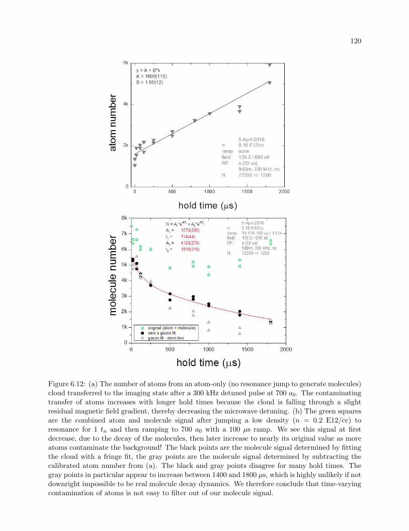
120

Figure 6.12: (a) The number of atoms from an atom-only (no resonance jump to generate molecules)cloud transferred to the imaging state after a 300 kHz detuned pulse at 700 a0. The contaminatingtransfer of atoms increases with longer hold times because the cloud is falling through a slightresidual magnetic field gradient, thereby decreasing the microwave detuning. (b) The green squaresare the combined atom and molecule signal after jumping a low density (n = 0.2 E12/cc) toresonance for 1 tn and then ramping to 700 a0 with a 100 µs ramp. We see this signal at firstdecrease, due to the decay of the molecules, then later increase to nearly its original value as moreatoms contaminate the background! The black points are the molecule signal determined by fittingthe cloud with a fringe fit, the gray points are the molecule signal determined by subtracting thecalibrated atom number from (a). The black and gray points disagree for many hold times. Thegray points in particular appear to increase between 1400 and 1800 µs, which is highly unlikely if notdownright impossible to be real molecule decay dynamics. We therefore conclude that time-varyingcontamination of atoms is not easy to filter out of our molecule signal.

121

Figure 6.13: (a) Microwave lineshapes of our low-density (n = 0.2 E12/cc) condensate with a 8 µs,9 dBm π-pulse after a 1 tn dwell time on resonance and a ramp time = 100 µs to 700 a0. Over1750 µs the frequency changes by 97 kHz. (b) The number of atoms transferred to the imagingstate by a 9 dBm, 300 kHz detuned 50 µs microwave pulse that tracked the microwave frequencyby 0.055 kHz/µs. We compare a Sine×Gaussian fringe fit (black points) to a normal Gaussian fit(gray triangles) and see good agreement in number. The number is roughly constant as a functionof time, therefore the linear tracking is a good approximation.

122

0 500 1000 1500 20000

2k

4k

6kN = A1*e

-t/t1 + A2*e-t/t2

A1 = 2230(420) t1 = 156(91)A2 = 4280(460) t2 = 2140(400)

sine x Gauss fit Gauss fit - atom line

12 April 2016n: 0.18 E12/ccramp: 10-510-100 us / 1.0 tnfield: 159.2 / 710 a0RF: s (50 us)

9dBm, 300 kHz, yes N: 75000 +/- 1600

mol

ecul

e nu

mbe

r

hold time ( s)Figure 6.14: The number of molecules after a 510 µs dwell time (∼ 1 tn for the n =0.2 E12/cccloud) on resonance and a 100 µs ramp to 700 a0 as a function of hold time, transferred to theimaging state with a 9 dBm, 300 kHz detuning 50 µs microwave pulse that tracked the detuningas the cloud fell. The black points represent the molecule number determined after separating theatoms from the signal using fringe fit analysis, the gray triangles represent the molecule numberdetermined after subtracting the calibrated, constant atom number.

123

6.2.4 Investigation into B-field noise

Frequency tracking is necessary to keep the transferred atom number constant as the cloud

falls, but it does not affect the transferred molecule number. Because the molecule signal has a

broad dissociation lineshape, and the molecules do not resassociate and therefore can be saturated,

the molecule signal can be made insensitive to small changes in the magnetic field. This is not true

for the transferred atom number.

Frequency tracking does not protect us from fluctuations in the transferred atom number due

to other magnetic field variations. Careful tuning of our coil driver current servos and meticulous

eddy current corrections have minimized our magnetic field noise to less than 10 mG, see figure

6.15. However, this magnetic field noise projects into ≤ 10% number noise! This projection is

calculated by the slopes of the transferred atom number over microwave detuning, these slopes are

501 atoms/kHz and 145 atoms/kHz at 200 kHz and 400 kHz detuning, respectively.

Because we treat the number of atoms as a constant, this noise has huge implications for

our perceived molecule signal, especially at short times when the magnetic field noise is maximum.

Rather than accept the consequences of these implications, we seek to avoid them altogether. We

have three options: (1) make the atoms less sensitive to the magnetic field, (2) reduce the magnetic

field noise, or (3) remove the magnetic-field sensitive atoms from the imaging process.

One could reduce the field-sensitivity of the atoms by changing the state transition for imag-

ing. Our beginning and final states must remain the same: atoms and molecules begin in |2,−2〉

and we image the molecules in |3,−3〉. The 2.6 GHz transition of |2,−2〉 → |3,−3〉 is sensitive

to the magnetic field, hence our noise problem [75]. However, if we first transferred our molecules

to the |2,−1〉 state (a 80 MHz transition that is significantly less sensitive to the magnetic field),

then the molecules could be transferred |3,−2〉 → |3,−3〉. This is the imaging process previously

employed to spectroscopically measure Tan’s contact in our lab [75]. However, the fast expansion of

the newly-seperated molecular atoms as they transfer through the multiple states, combined with

the already low-signal, results in clouds too sparse to properly image. There are also implications

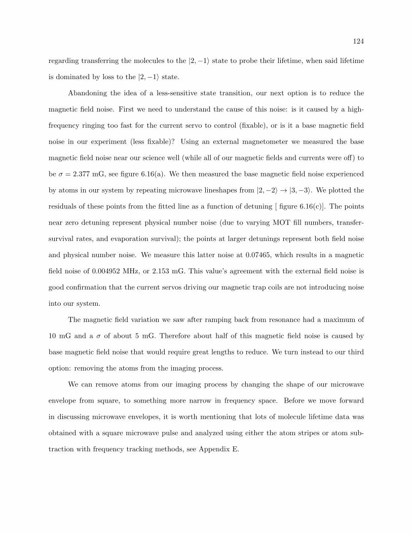
124

regarding transferring the molecules to the |2,−1〉 state to probe their lifetime, when said lifetime

is dominated by loss to the |2,−1〉 state.

Abandoning the idea of a less-sensitive state transition, our next option is to reduce the

magnetic field noise. First we need to understand the cause of this noise: is it caused by a high-

frequency ringing too fast for the current servo to control (fixable), or is it a base magnetic field

noise in our experiment (less fixable)? Using an external magnetometer we measured the base

magnetic field noise near our science well (while all of our magnetic fields and currents were off) to

be σ = 2.377 mG, see figure 6.16(a). We then measured the base magnetic field noise experienced

by atoms in our system by repeating microwave lineshapes from |2,−2〉 → |3,−3〉. We plotted the

residuals of these points from the fitted line as a function of detuning [ figure 6.16(c)]. The points

near zero detuning represent physical number noise (due to varying MOT fill numbers, transfer-

survival rates, and evaporation survival); the points at larger detunings represent both field noise

and physical number noise. We measure this latter noise at 0.07465, which results in a magnetic

field noise of 0.004952 MHz, or 2.153 mG. This value’s agreement with the external field noise is

good confirmation that the current servos driving our magnetic trap coils are not introducing noise

into our system.

The magnetic field variation we saw after ramping back from resonance had a maximum of

10 mG and a σ of about 5 mG. Therefore about half of this magnetic field noise is caused by

base magnetic field noise that would require great lengths to reduce. We turn instead to our third

option: removing the atoms from the imaging process.

We can remove atoms from our imaging process by changing the shape of our microwave

envelope from square, to something more narrow in frequency space. Before we move forward

in discussing microwave envelopes, it is worth mentioning that lots of molecule lifetime data was

obtained with a square microwave pulse and analyzed using either the atom stripes or atom sub-

traction with frequency tracking methods, see Appendix E.

125

Figure 6.15: The measured magnetic field after a ramp time = 100 µs from resonance to 700 a0.The measured microwave lineshape centers as a function of hold time at 700 a0 after a ramp time =100 µs back from resonance. The red line is a linear line on a lin-log plot representing the expectedchange due to the cloud falling. Deviation from this line is a representation of the magnetic fieldnoise. (b) The predicted effect of the magnetic field noise on the number of atoms transferred tothe imaging state as a function of hold time at unitary for 200 kHz detuning (black points) and300 kHz detuning (open circles), which are the detunings used to image molecules at 1000 a0 and700 a0, respectively. At 200 kHz detuning this magnetic field noise could transfer 250 fewer atoms,or about 10% of our overall signal.

126

Figure 6.16: (a) The magnetic field measured in the x (yellow), y (blue) and z (pink) axes. Thebase field oscillates on a 120 kHz frequency (consistent with power line noise) with σ = 2.377 mG.(b) The normalized number of atoms transferred to the imaging state as a function of RF detuning.(c) The residuals from (b) vs detuning. At zero detuning this noise represents the noise in numberfrom shot to shot, σnum = 0.04969 , while the noise at larger detunings represents the magneticfield noise in conduction with number noise, σcomb = 0.07465.

127

6.3 Microwave envelopes to suppress atom transfer

Our molecule images are contaminated by atoms because the far-detuned square microwave

pulse transfers off-resonant atoms to the imaging state. This transfer occurs because the corre-

sponding instrument function (i.e. the Fourier transform) of a square pulse is a sinc function, and

the oscillatory wings of a sinc function have appreciable amplitude, even at large detunings:

sq(t) = Aif(−T/2 ≤ t ≤ T/2)

F (ω) =1

2π

∫ ∞−∞

sq(t)e−iωtdt

=A

2πsinc (ω/2)

(6.5)

In this section we will examine two candidate envelopes for our microwave pulses whose frequency

components fall off much faster with detuning than our standard square envelope.

6.3.1 Long Gaussian pulses

A Fourier-transformed Gaussian is still a Gaussian, and therefore a microwave pulse with a

Gaussian-amplitude envelope is much more narrow in frequency space than a square pulse.

G(t) = Aet2

2σ2

F (ω) =1

2π

∫ ∞−∞

G(t)e−iωtdt

= Aσe−ω2σ2/2

(6.6)

Chapter 4 of [75] discusses past lab procedures to create Gaussian microwave pulses using a linear

variable gain amplifier to combine the outputs of a high frequency synthesizer and an arbitrary

function generator. Nowadays we have combined the high frequency and envelope generation into

one Agilent N5181A signal generator.

Our Gaussian pulse has a width characterized by σ = 50µs. We truncate the signal at

±3σ, so the entire pulse is 300 µs. There is no saturation and very little delay after sending our

signal through a 10 W amplifier, see figure 6.17. When detuned by ≥ 200 kHz this Gaussian pulse

transfers practically no atoms to the imaging state, we are therefore able to discern the molecular

lineshape from the atom lineshape, see figure 6.18.

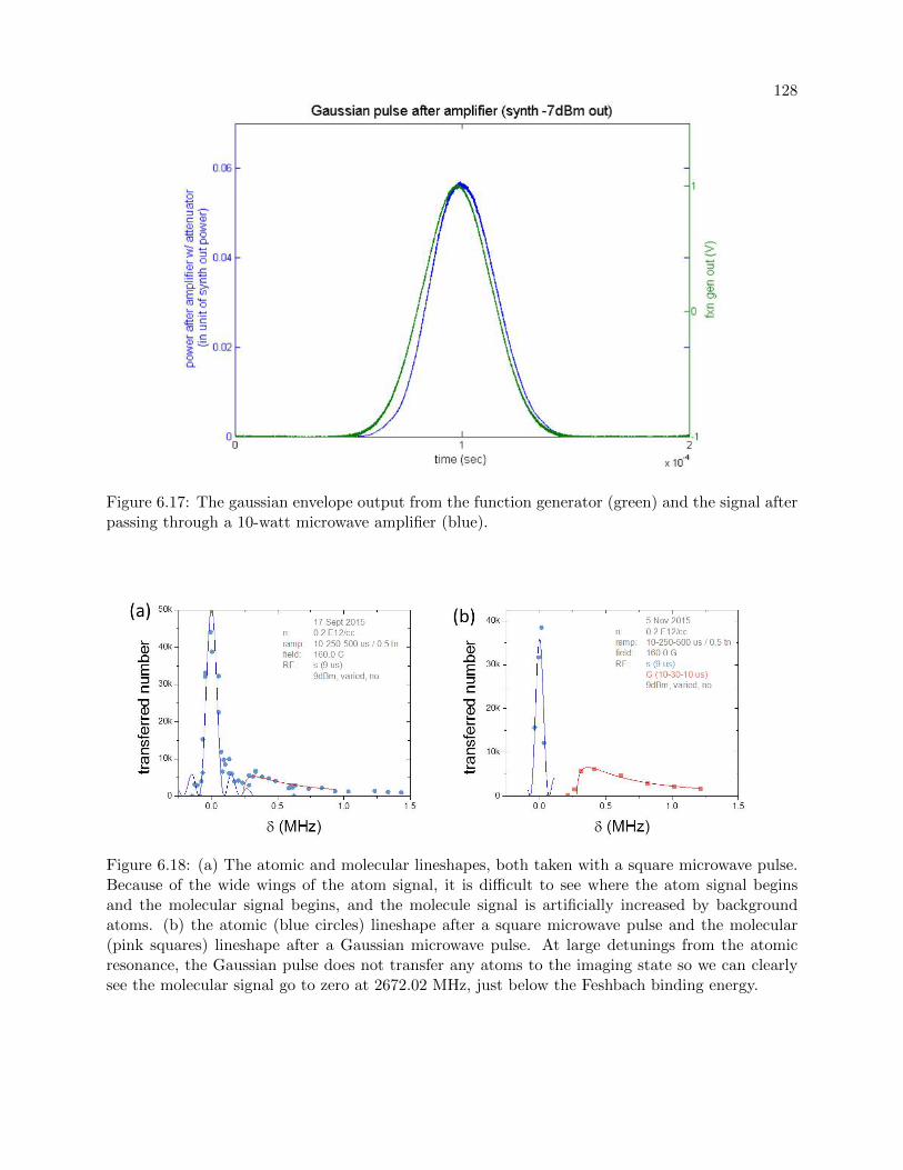
128

Figure 6.17: The gaussian envelope output from the function generator (green) and the signal afterpassing through a 10-watt microwave amplifier (blue).

Figure 6.18: (a) The atomic and molecular lineshapes, both taken with a square microwave pulse.Because of the wide wings of the atom signal, it is difficult to see where the atom signal beginsand the molecular signal begins, and the molecule signal is artificially increased by backgroundatoms. (b) the atomic (blue circles) lineshape after a square microwave pulse and the molecular(pink squares) lineshape after a Gaussian microwave pulse. At large detunings from the atomicresonance, the Gaussian pulse does not transfer any atoms to the imaging state so we can clearlysee the molecular signal go to zero at 2672.02 MHz, just below the Feshbach binding energy.

129

Figure 6.19 compares molecule data acquired by square and Gaussian microwave pulses as a

function of the ramp rate out. We see very little difference in the data. The implications of molecular

ramp out data is explored further in Chapter 7. More molecule data taken with Gaussian pulses

can be found in Appendices F and G.

Because the molecular dynamics we wish to study occur on a fast time scale (order of 100 µs),

the 300 µs pulse length of the Gaussian pulse makes it not ideal for molecule lifetime measurements.

While we could truncate our Gaussian pulse to be shorter with only minimal effects to its width

in frequency space, the Gaussian pulse does not provide enough power to saturate the molecule

signal in a timely manner. Whereas the square pulse emitted full power for its entire duration, the

Gaussian pulse emits full power for a small fraction of its duration. We therefore explore a second

envelope that can emit more power, quickly, while still keeping frequency width low.

130

0 50 100 150 2000

2k

4k

6k

8k

7/8 June 2016n: 5.5 E12/ccramp: 10-dwell-ramp / 0.5 tnfield: 160.0 / 496 a0RF: G (300 us) / no hold

s (50us) / 50 us hold9dBm, 400 kHz, yes

N: 78000 +/- --70000 +/- --

ramp out ( s)

mol

ecul

e nu

mbe

r

Figure 6.19: The molecule number as a function of ramp out rate after transfer to the imagingstate by a square (blue circles) or a Gaussian microwave pulse (pink squares). There is very littledifference between the two datasets.

6.3.2 Short curved pulses

A good compromise between the frequency-succinct yet temporally long Gaussian pulse, and

the temporally-succinct yet frequency-wide square pulse, is a square pulse with curved edges. In

this “curved pulse” the non-negligible duration of maximum power present in the square pulse

is maintained by a flat top of maximum microwave power, yet the high-frequency components

associated from the sharp, square edges are reduced, see figure 6.20(a).

The curved pulse envelope is based off the Blackman function:

B(t) =21

50+

1

2cos

[πt

σ

]+

2

25cos

[2πt

σ

]. (6.7)

131

The corresponding instrument function is a sinc function divided by powers of σ up to σ4:

F (ω) =1

2π

∫ ∞−∞

B(t)e−iωtdt

=a(0.84− 0.36σ2ω2) sinc(2πσω)

(1− σ2ω2)(1− 4σ2ω2)

(6.8)

[87]. The reduced frequency components of this function are ideal, however this function alone has a

short peak, much like a Gaussian. For our purposes, we want to blast the molecules with maximum

microwave power for a prolonged period in order to saturate molecule signal. We therefore defined

our curved pulse envelope by the following piecewise function:

c(t) =

A/10000 if t < −(τ1 + τ2)/2

A(

12 cos

[2π(t−(τ1−τ2)/2)

2 − 1]

+ 0.08 cos[

2π(t−(τ1−τ2)/2)2 − 1

]+ 0.42

)if −(τ1 + τ2)/2 ≤ t ≤ −τ2/2

A if −τ2/2 < t < τ2/2

A(

12 cos

[2π(t−(τ1+τ2)/2)

2 − 1]

+ 0.08 cos[

2π(t−(τ1+τ2)/2)2 − 1

]+ 0.42

)if τ2/2 ≤ t ≤ −(τ1 + τ2)/2

A/10000 if t > (τ1 + τ2)/2,

(6.9)

where τ1 and τ2 define the rise (fall) time and persist time, A is the amplitude of the signal and

A/10000 is effectively zero. We find that a rise time of 10 µs and a persist time of 30 µs transfers less

than 1% of atoms to the imaging state for detunings ≥ 225 kHz (for 200 kHz, we set τ1 = 15 µs),

this results in a full pulse length of 50 (60) µs. We record the times of curved pulses as (rise -

persist - fall) time, e.g. the pulse described above is (10-30-10 µs).

Because this signal follows a piecewise function with a fast frequency rising time, we are

unable to generate this amplitude envelope on our Agilent synthesizer. We instead generate the

envelope as a voltage on a function generator (Agilent 33522A) and use a gain amplifier (ADL5330)

to combine the synthesizer’s microwave frequency with the curved voltage envelope. The amplifier

has non-linear gain, especially at high power, that we must calibrate into our envelope. For a

desired waveform voltage of c(t), the output of the amplifier is

0.28654 + 0.9441eV(t)−4.39056

43.48201 + 1.1326 · 10−7eV(t)−4.39056

0.27742 , (6.10)

132

Figure 6.20: (a) Our curved pulse with an amplitude of for a (5-45-4µs) pulse (orange) comparedto a 50 µs square pulse (blue). (b) The Fourier transform of our curved pulse (orange) compared toa square pulse (blue). The high frequency components of our curved pulse fall off much faster thanthat of a square pulse. The inset shows the same plot on a log scale, on which it is easier to see thatthe percentage of atoms of transferred with our curved pulse is only 1.5% at 200 kHz detuning, 0.1%at 300 kHz detuning, and 0.01% at 400 kHz. At this largest detuning this percentage correspondsto only 7 atoms, a significant decrease from the 700 atoms (1%) transferred with a square pulse.

where V(t) is the variable gain amplifier input voltage,

V (t) = 10 + 20 log(c(t)). (6.11)

133

Figure 6.21 compares molecule lifetime data taken with our curved pulse to that taken with a

square pulse. The curved pulse has overall less number because, unlike the square pulse data, only

a negligible number of atoms transfer to the imaging state. Without these field-sensitive atoms in

the image background, the curved-pulse dataset also has greater signal to noise, resulting in smaller

lifetime fit errors.

0 500 1000 1500 20000

1k

2k

3k

4k

5k

6kN = A

1*e-t/t1 + A

2*e-t/t2 + y

0

y0 = 903 0

A1 = 1160(310) 610(130)

t1 = 134(77) 84(42)

A2 = 2890(320) 3220(120)

t2 = 2370(630) 1790(150)

atom offset: 71300 x 63.3% x 2% = 903

9 May 201629 July 2016

n: 0.18 0.167 E12/ccramp: 10-756 760-100 us / 1.5 tnfield: 159.2 / 706 700 a0RF: sq (50 us)

c (10-30-10 us)9dBm, 300 kHz, yes

N: 71300 +/- 220073000 +/- 1100

mol

ecul

e nu

mbe

r

hold time ( s)

Figure 6.21: The number of molecules (and atoms) imaged after a (10-30-10 µs) curved RF pulse(green triangle) or a 50 µs square RF pulse (blue point) after a tdwell = 1.5 tn evolution on resonanceand ramp time = 100 µs to 700 a0. Both datasets account for the falling cloud with frequencytracking. In addition to the molecules, there are about 900 atoms transferred to the imaging statefor the square dataset.

134

6.4 Imaging settings for molecules

Once the molecules are spin flipped to the imaging state they are imaged using standard

absorption imaging procedures. Because the optical depth of these clouds are usually lower than

2, high-intensity imaging is not needed.

Because we are not using high-intensity imaging, epsilon correction due to varying AOM

power is not pronounced (see Chapter 3). We analyzed our molecule data by both (1) fast 2D

Gaussian fits and (2) azimuthally averaging the 2D images then subtracting residual backgrounds,

as outlined in Chapter 3. We did not see appreciable difference in the size or number of the

molecule clouds, and therefore most of the remaining molecule data in this thesis is processed using

2D Gaussian fits.

Chapter 7

Molecule formation

Having realized the production of molecules, we now attempt to understand how these

molecules are produced. In this chapter we will discuss a simple model to predict the number

of molecules as a function of ramp out, then compare predictions to measurements. We will then

discuss the more mysterious dependency on dwell time, for which we have no model. Finally we

will discuss corrections and limitations to our model.

7.1 A simple ramp-out model

We present now a simple theory to explain the molecule production during the ramp back

from resonance. This model is based heavily on the model developed by Altman and Vishwanath

to describe the production of Feshbach molecules in Fermi systems when rapidly sweeping away

from the Feshbach resonance [88]. Our system differs in that we are working with Bosons.

When applying this model to our system it is best to think of the resonant atoms as in a

superposition of the two states present at unitarity, see figure 7.1. While the bound Feshbach state

technically ceases to exist on resonance, this model assumes the existence of a higher momentum

free atom state that we suppose is about 1 En higher in energy than the ground many-body state.

These states are modeled as an avoided crossing.

The model supposes that fast sweeps across the resonance can be divided into two stages:

a “sudden” stage and an “adiabatic” stage. The sudden stage is approximately an infinitely fast

sweep, meaning that the initial state is simply projected onto the final state; during this stage the

136

Figure 7.1: We can use an avoided crossing metaphor to explain molecular formation. We havetwo states, gray and blue, whose avoided crossing switches their spins; in thos metaphor, the rightside of the spin up and spin down states represent our free atom and bound molecule states. (a)For an infinitely rapid jump that begins from the spin-up blue state, the system hops across theavoided crossing and maintains in the spin-up configuration. (b) A gradual adiabatic change allowsthe system to adapt its spin such that it can remain in the blue state. (c) If we now begin in theblue state near the avoided crossing, we begin in a superposition of spin up and spin down. Anadiabatic ramp away from the avoided crossing would allow the state to adapt to spin down andremain in the blue state. (d) If we begin in a superposition of both the gray and blue states onresonance, an adiabatic ramp away from the avoided crossing would separate the cloud into blueand gray states. Likewise, a sudden jump away from the avoided crossing could result in the entiresystem projecting onto only the blue or gray state, depending on the phase of the superposition.

resonance wave function is projected into molecular and atomic components. Our ramp is in the

adiabatic stage after Eb < E2b (Eb is defined in equation 2.9); during this stage the projected atoms

and molecules are simply dragged to the final B field value, see figure 7.2.

137

Figure 7.2: Our resonant condensate may be in a superposition of a ground and excited energystate which translate into the free atom and molecular bound state at larger magnetic fields. Theramp away from resonance is at first sudden but becomes adiabatic at B(a∗), represented by thedashed line. The two-state superposition model is an oversimplification of our actual system, asthere are more unbound states present on resonance. And we will discuss later how not all theresonant atoms seem to be in a superposition of the bound and unbound states, i.e. only someatoms have the propensity to be swept into molecules.

The scattering length at which the sweep converts from sudden to adiabatic is a∗, defined by

Eb(a∗) = E2b(a∗). In [88], they make the linear assumption a(B) = α

B−B0, where α = mg2

4π∆µ , g is the

coupling between open and closed channels and ∆µ is the difference in magnetic moment between

the open and closed channels. This linear approximation is valid near the resonance, where α is

138

approximately 4000 a0 G. With the linear assumption of a, a∗ becomes

a∗ =

(α~

4mB

)1/3

. (7.1)

We see that the value of a∗ ∝ (B)−1/3. This means that for a constant ∆B, a longer ramp time

yields a larger value of a∗, see figure 7.3. We assume a linear ramp speed of B = (5/4)∆B /rout.

We multiply this ramp rate by 5/4 for reasons explained in Chapter 5.

Figure 7.3: Calculations of a∗ assuming a linear approximation of a(B), as a function of ramp timefor constant ∆B (because we define ramp time in relation to B −B0, the actual value of ∆B doesnot change this plot). a∗ is larger for slower ramp times, indicating that a greater percentage ofthe total ramp time is adiabatic.

The sudden approximation theory dictates that the number of molecules formed is equal to

the initial resonance wave function projected onto the wave function at a∗. If we assume that the

139

wave functions are of e−r/a/r form, the number of molecules projected is then

Nmol =N

2

∫1√

2πa∗

e−r/a∗

r· 1√

2πa′e−r/a

′

r· 4π r2 dr, (7.2)

where a′ represents the interactions on resonance that are currently unknown. This integral sim-

plifies to

Nmol =N

2

2√a∗√a′

a∗ + a′. (7.3)

If a′ a∗, as is true for very fast ramps, this simplifies further to 4a∗/a′.

If we assume universal scaling with density in our resonant condensates, we can then suppose

that the size of the molecule-like state on resonance is proportional to the inverse of universal

momentum κn such that

a′ = s(6π2n)−1/3, (7.4)

where s is a scaling factor that we will for now set to 1. The predicted n−1/3 dependence in a′

translates into density dependence of Nmol, see figure 7.4.

140

Figure 7.4: The calculated fraction projection of molecules, Nmol/N , equation (7.3), as a functionof rout for constant ∆B. The modeled clouds have initial densities of 0.2 (red) and 5 (blue) E12/cc,using equations (7.1) and (7.4).

7.2 Data

7.2.1 Molecule number vs rout

We measured the number of molecules as a function of rout for clouds of initial densities of 5.5

and 0.18 E12/cc after spending tdwell = 1.4 tn on resonance then ramping away to 160 G , see figure

7.5. The molecules were transferred to the imaging state by a long (300 µs) Gaussian-enveloped

microwave pulse detuned 400 kHz from the atom resonance (see Chapter 6 for more information

about microwave transfers). We fit this data by eye (no χ2) with equation (7.3) (assuming equation

(7.4) to be true) and including a proportionality factor of Cfit. We find that the data are well

described by this equation when Cfit = 0.1, meaning that about 10% of the resonant atoms have

the propensity to be swept into molecules, or 90% of the atoms are not in the superposition resonant

141

state of our rough model in figure 7.2. This data therefore serves as good evidence for universal

scaling with density at unitarity.

0 200 400 600 8000.00

0.05

0.10

13 Jan 2016n: 5.5 0.18 E12/ccramp: 10-dwell-ramp us / 1.5 tnfield: 160 GRF: G (300us)

9dBm, 400 kHz, no N: 53500 +/- --

rout ( s)

Nm

ol /

N

Figure 7.5: The fractional number of molecules, Nmol/N , measured after tdwell = 1.5 tn on resonanceand a ramp away to 160 G at various rout rates, for initial densities of 5.5 (dark blue points) and0.18 (cyan triangles). The dashed lines are equation (7.3) combined with equations (7.1) and (7.4)including a proportionality factor of 0.1. We see good agreement between the predictions anddata, this encourages not only our application of the superposition ramp-out model but also ourassumption of universal scaling with density to predict a′. The abbreviated legend in the bottomright is explained in Appendix A.

While the projection model predicts that 100% of the atoms can be swept into molecules (such

that Nmol/N saturates to 50%, see figure 7.4), we saw our molecule signal saturate at only 10%

(see figure 7.5). This begs the question of whether the time on resonance affects the propensity

of the atoms to be swept into the molecule state. Unfortunately, not all data is as agreeable

142

with our universal arguments. Ramp out data of tdwell = 0.5 tn (all other experimental settings

unchanged) is plotted in figure 7.6. The dashed lines are the same as in figure 7.5, using equation

(7.3) and assuming equation (7.4) to be true, with Cfit = 0.1. While we expect to see a change

of Cfit, we instead find that the number of atoms projected into the molecular state no longer

varies with density as expected. This indicates that the interactions on resonance are not fully

explained by our simple approximation in equation (7.4) and perhaps evolve on resonance in a not

fully density-universal manner. This strange behavior is explored further in Chapter 9.

143

0 200 400 600 8000.00

0.05

0.10

rout ( s)rout ( s)rout ( s)

13 Jan 2016n: 5.5 0.18 E12/ccramp: 10-dwell-ramp us / 0.5 tnfield: 160 GRF: G (300us)

9dBm, 400 kHz, no N: 53500 +/- --

Nm

ol /

N

Figure 7.6: The fractional number of molecules, Nmol/N , measured after tdwell = 0.5 tn on resonanceand a ramp away to 160 G at various rout, for initial densities of 5.5 (dark blue points) and 0.18(cyan triangles). The dashed lines are the same predictions plotted in figure 7.5. We see that theprojected number of molecules no longer varies with density in the expected manner consistentwith universal scaling with density. This indicates that the interactions on resonance are not fullyexplained by our simple assumption of equation (7.4).

7.2.2 Comparing atom loss with molecule formation

From our ramp-out data we reach the unfortunate (but interesting?) conclusion that molecules

are produced even for our fastest ramps away from resonance. The resonant atom loss data in Chap-

ter 5 is therefore not purely loss during resonance, but a sum of atom loss to deeply bound dimers

while on resonance and atom loss to shallow dimers during the sweep to weak interactions. While

we cannot quantify the percentage of atom loss due to the shallow dimer production with an exact

144

number, we can estimate an upper limit.

We measured the number of molecules produced out of an N = 73800 ± 4300 condensate

after tdwell = 1 tn on resonance and rout = 10 µs to 160 G. About 2983 ± 33 molecules formed

out of an initially low density cloud (n = 0.208 E12/cc) and 2791 ± 173 molecules form out of

a standard density cloud (n = 5.78 E12/cc). This corresponds to 8.1 and 7.6 % of the atoms in

the low and standard density clouds being swept into shallow dimers. The atom loss reported in

Chapter 5 (rout = 5 µs to 163 G) between n = 0.211 and n = 0.302 E12/cc had an average loss of

17.6 %, while data at n = 3.07 and n = 6.03 E12/cc had an average loss of 15.85%.

Comparing the 10 µs molecule ramp to the 5 µs atom ramp over-estimates the percentage

of atoms swept into the molecular states. This data is also skewed by the different ∆B (5 G for

molecule data, 8 G for atom data), which affects the extent of the linear regime of the magnetic

ramp, see equation (5.1). However, from this comparison we can estimate that up to 46 and 48

% of the atom loss observed in the low and standard density clouds was due to ramping molecule

formation - i.e. nearly half of the atom loss was to shallow dimers! This number is large not

because Nmol is large, but because the amount of atom loss is low. We expect this percentage to

vary with dwell time both because the atom loss increases with dwell time, and because the number

of molecules also varies significantly.

7.3 Dwell time dependencies

As was discussed in section 7.2.1, our simple sweep model cannot explain how the propensity

of atoms to be swept into molecules is influenced by the evolution on resonance. To explore this

experimentally, we measured the number of molecules produced by a rout = 50 µs to 160 G after

various dwell times on resonance, see figure 7.7. We found that the number of molecules first

increases with dwell time, indicating that the propensity to be swept into molecules is a feature

that evolves on resonance, possibly at a universal density rate that scales with tn. At longer dwell

times however, the number of molecules begins to fall. Unlike the formation rate, this decay rate

does not appear to scale with tn, but is rather constant in absolute time units. It is unclear from

145

this data whether this drop in molecule number arises from decay of dimer-prone resonant atoms to

deeply bound states, or from the dimer-prone atoms evolving back into atoms that are not dimer-

prone. While corresponding returned atom data never showed an upswing of atoms that would

support the latter hypothesis, there was a flattening in the decay rate at similar times that was

suspiciously close to, yet ultimately below our signal to noise, see figure 5.25.

146

Figure 7.7: The molecule number produced after a resonant cloud of n = 0.2 (cyan), 5 (blue), and18.8 (black) E12/cc is ramped to 160 G at rout = 50 µs, as a function of dwell time on resonance.(a) The data plotted in universal units of tdwell/tn. (b) The same data plotted in absolute timeunits. The number of molecules first increases with dwell time at universal rate, but later decreasesat a rate independent of density.

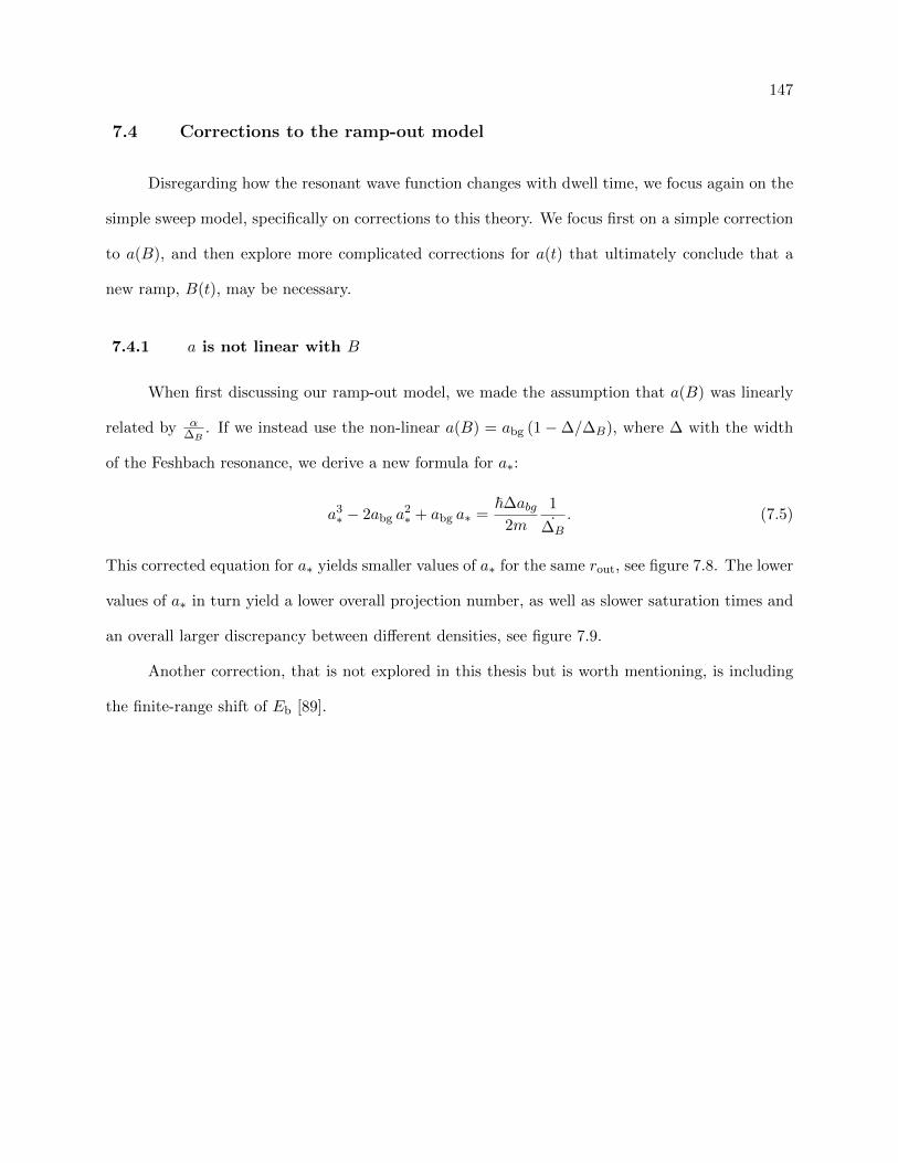
147

7.4 Corrections to the ramp-out model

Disregarding how the resonant wave function changes with dwell time, we focus again on the

simple sweep model, specifically on corrections to this theory. We focus first on a simple correction

to a(B), and then explore more complicated corrections for a(t) that ultimately conclude that a

new ramp, B(t), may be necessary.

7.4.1 a is not linear with B

When first discussing our ramp-out model, we made the assumption that a(B) was linearly

related by α∆B

. If we instead use the non-linear a(B) = abg (1−∆/∆B), where ∆ with the width

of the Feshbach resonance, we derive a new formula for a∗:

a3∗ − 2abg a

2∗ + abg a∗ =

~∆abg2m

1

∆B

. (7.5)

This corrected equation for a∗ yields smaller values of a∗ for the same rout, see figure 7.8. The lower

values of a∗ in turn yield a lower overall projection number, as well as slower saturation times and

an overall larger discrepancy between different densities, see figure 7.9.

Another correction, that is not explored in this thesis but is worth mentioning, is including

the finite-range shift of Eb [89].

148

Figure 7.8: The calculated a∗ as a function of rout for constant ∆B, assuming a linear a(B)approximation (orange) given by equation (7.1), or a more accurate a(B) relation (gray) given byequation (7.5). The latter has lower values of a∗, meaning that more of the total ramp time isadiabatic, and therefore predicts that less atoms will be swept into the shallow molecule state.

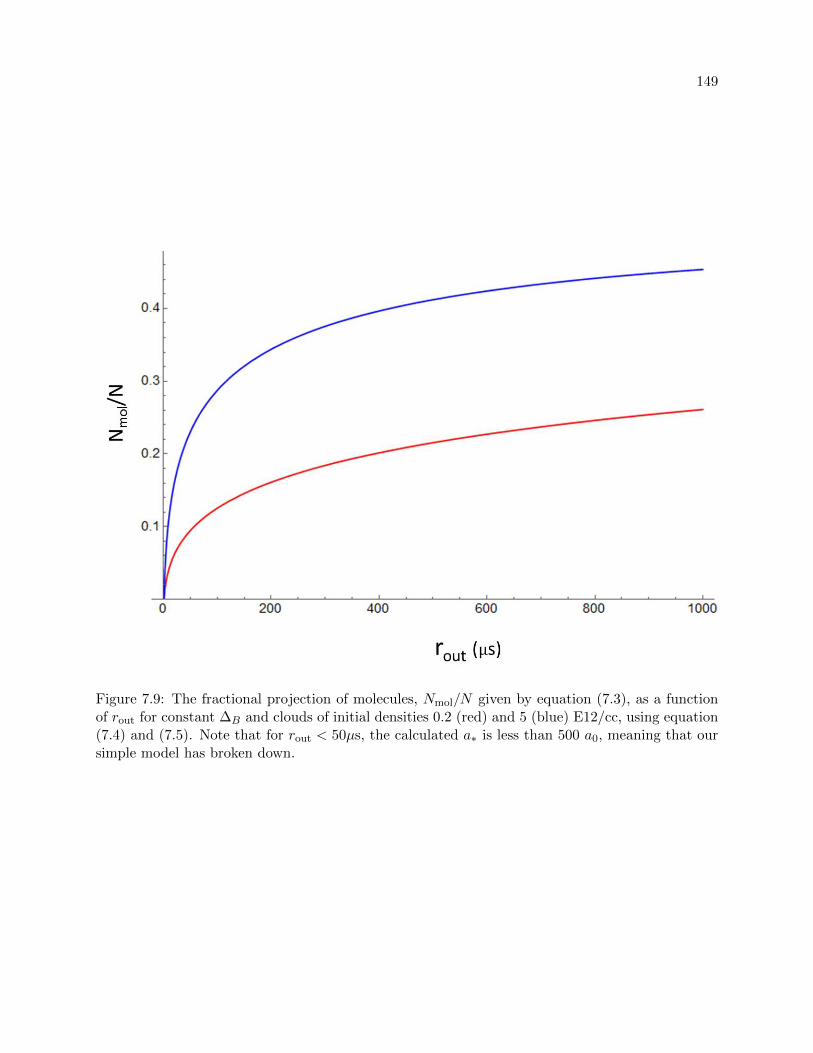
149

Figure 7.9: The fractional projection of molecules, Nmol/N given by equation (7.3), as a functionof rout for constant ∆B and clouds of initial densities 0.2 (red) and 5 (blue) E12/cc, using equation(7.4) and (7.5). Note that for rout < 50µs, the calculated a∗ is less than 500 a0, meaning that oursimple model has broken down.

150

7.4.2 Non-linearities in B(t)

In Chapter 5 we discussed the actual shape of our magnetic ramp, B(t). Most importantly, we

discussed how the linear regime of B(t) exists only between 0.125 and 0.875 ∆B. This is important

now because we ramp our atom and molecule data out to different final values of B (for imaging

reasons). Although we compensate rout in order to keep the linear rate (B) the same regardless of

∆B, this does not properly correct B(t) in the non-linear regime. For our fastest ramps, a∗ can

occur in the non-linear regime. The non-linear regime composes the first and last 12.5% of our

magnetic ramps. When ramping from resonance to 163 G, as we do when imaging atoms, this

means that only between 4560 and 240 a0 is the ramp linear. This constrains our minimum rout to

only 20 µs to keep a∗ in the calculable linear regime, or about 4 times slower than our maximum

speed. (Note: this maximum speed was calculated using equation (7.5), if we assume the linear

approximation of equation (7.1), then the minimum rout is extended to a non-constraining 0.5

µs). However, when ramping to 160 G, as we do when imaging molecules, the ramp is linear only

between 7040 and 650 a0, which constrains our minimum rout to only 105 µs!

It is very difficult to extract the dependency of a∗ on rout when B(t) is non-linear. Moreover,

the ramp-out model we use here is a simple approximation, and therefore changing our ramp rates

to keep a∗ at nearly the same value as we vary ∆B to compare atom and molecule number is

frivolous. We therefore conclude that the best course of action for further study of ramp out effects

is to design a new ramp, B(t), that better suits the needs of our system. We do not explore this

option further in this thesis. For now, we shift our focus to the properties of the molecules that

have been formed, regardless of the ramp out rate.

Chapter 8

Molecule lifetime measurements

8.1 Two-component decay

This chapter describes our studies of molecules created after spending tdwell = 1.5 tn on

resonance and ramping away at rout = 100 µs to af . We measure the lifetime by measuring the

molecule number as a function of hold time at af . Figure 8.1 shows this number decaying at

af = 700 a0 for clouds of two different initial densities, n = 0.208 and n = 1.32 E12/cc. Neither

dataset can be described by a single exponential decay rate, as would be expected for a simple gas

of Feshbach dimers. They instead fits well to a sum of two exponential decays:

A1 × e−t/t1 +A2 × e−t/t2. (8.1)

Spontaneous dissociation, such as spin relaxation into a lower spin state, would appear as a

simple exponential decay in our data. Non-exponential decay would be present if there was also

inelastic loss, such as molecule-molecule collisions. Such inelastic loss would be density-dependent,

and would therefore be less pervasive at lower densities. Because figure 8.1 shows two-component

loss where the fast component does not vary with density, despite the density varying by more

than a factor of 6, we can safely conclude that this non-exponential loss is not due to inelastic loss

mechanisms.

We investigated this loss further by measuring the molecular decay rates for more values of

density and af ; some of this data is shown in figure 8.2. When this data is analyzed by a two-

exponent sum, the faster of the two loss rates is unchanged by both af and initial density. The

152

Figure 8.1: The molecule number measured as a function of hold time at af = 700 a0 for initialcloud densities of n = 0.208 E12/cc (purple points) and 1.32 E12/cc (blue triangles). This datais best fit by a sum of two exponentials, the fit values for each dataset are included in the lowerleft corner of the plot. The fast loss for each dataset is equal within error, while the slower loss ofeach dataset is slower in the lower density dataset. The abbreviated legend in the upper right isexplained in Appendix A.

decay rate of the slower loss (1/t2), however, appears to decrease with larger af and increase with

larger n. We will now investigate the dependencies of this slower loss.

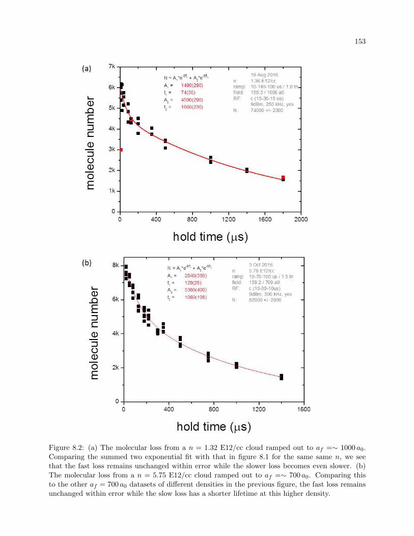
153

Figure 8.2: (a) The molecular loss from a n = 1.32 E12/cc cloud ramped out to af =∼ 1000 a0.Comparing the summed two exponential fit with that in figure 8.1 for the same same n, we seethat the fast loss remains unchanged within error while the slower loss becomes even slower. (b)The molecular loss from a n = 5.75 E12/cc cloud ramped out to af =∼ 700 a0. Comparing thisto the other af = 700 a0 datasets of different densities in the previous figure, the fast loss remainsunchanged within error while the slow loss has a shorter lifetime at this higher density.

154

8.2 Dimers: the slow decay

8.2.1 Dimer lifetime predictions

At 700 a0 the Feshbach molecules are bound by about 110 kHz in the |2,−2〉 state. These

molecules can spontaneously dissociate via spin relaxation into the |2,−1〉 and |2, 0〉 states [90],

which are 79.62 and 75.49 MHz away, see figure 6.1. This lifetime due to this spontaneous dissoci-

ation varies with af but not density, and is calculated in [90] to be

τD(B) = τres

m a2bg µres ∆

2 ~2

(B −B0

∆

)2( ∆

B −B0− 1

)3

, (8.2)

where abg, B0 and ∆ are all Feshbach resonance parameters defined in Chapter 2, µres/h = 34.66

MHz/mT and τres = 32µs. In terms of af , τD becomes:

τD(a) = τresm abg µres ∆

2 ~2

−a3

(abg − a)2, (8.3)

this decay rate is plotted in figure 8.3.

Density dependence is introduced into the predicted dimer lifetime by inelastic atom-dimer

collisions. An atom-dimer scattering event occurs when an unbound atom collides with a shallow-

bound Feshbach molecule, producing a deeply bound molecule and recoiling atom [66, 91]. This loss

is enhanced by the presence of the three-body Efimov state, as it increases the probability for an

atom to be near a dimer. This loss rate has been measured experimentally by many [58, 59, 57, 60],

and is defined by the atom-dimer collisional rate coefficient, β, calculated in [92] to be

β(a) =20.3 sinh(2η∗)

sin2 [s0 ln(a/a∗)] + sinh2 (η∗)

~am, (8.4)

where a∗ is the scattering length at which the Efimov state intersects the atom-dimer threshold

(creating a loss rate resonance), and η∗ is the inelasticity parameter characterizing the width of the

Efimov resonance at a = a∗. For 85Rb, η∗ was measured in [34] to be 0.057. a∗ for the first-excited

Efimov state was calculated in [66] to be ∼ 275 a0.

The lifetime determined by the atom-dimer collisional rate is then

τAD =1

n′β(8.5)

155

where n′ is the adjusted density after calibrating for the atoms lost while on resonance. For

tdwell = 1.5 tn, n′ = 0.7n for almost all densities. Because there are many more atoms than

molecules in our system, the fractional atom loss is small and n′ therefore remains nearly constant

during hold time; this makes the density-dependent inelastic loss appear as a simple exponential

decay in our systems. This loss rate is plotted in figure 8.4 as a function of adjusted cloud density,

n′.

We can now define our total predicted lifetime, defined by the inverse of the loss rate, by

combining the collisional and spontaneous decay rates:

1

τTotal(a, n)=

1

τD(a)+

1

τAD(a, n′). (8.6)

This combined inverse loss rate is plotted as a function of af for three initial densities in figure 8.5.

Figure 8.3: The dimer lifetime considering only loss due to spontaneous dissociation into the lowerspin state as a function of af .

156

Figure 8.4: The dimer lifetime considering only loss due to inelastic atom-dimer collisions as afunction of density, for a = 700 a0.

157

500 1000 1500 20000.01

0.1

1

10

a (a0)

Tota

l (ms)

Figure 8.5: The total predicted dimer lifetime considering both spontaneous dissociation and inelas-tic atom-dimer collisions for atom+molecule clouds of initial density n = 0.2 (red), 1.3 (blue) and5.8 (green) E12/cc. The dashed line represents the dimer lifetime predicted by spontaneous disso-ciation only. The lowest density curve follows the lifetime set by spontaneous dissociation becauseit is the least influenced by atom-dimer collisions. We that at af ∼ 275 a0 the lifetimes decreasedramatically due to the atom-dimer collision resonance near a∗. At larger scattering lengths we seethe total lifetime again begin to decrease, this is due to the next atom-dimer collision resonancelocated at 22.7 × a∗.

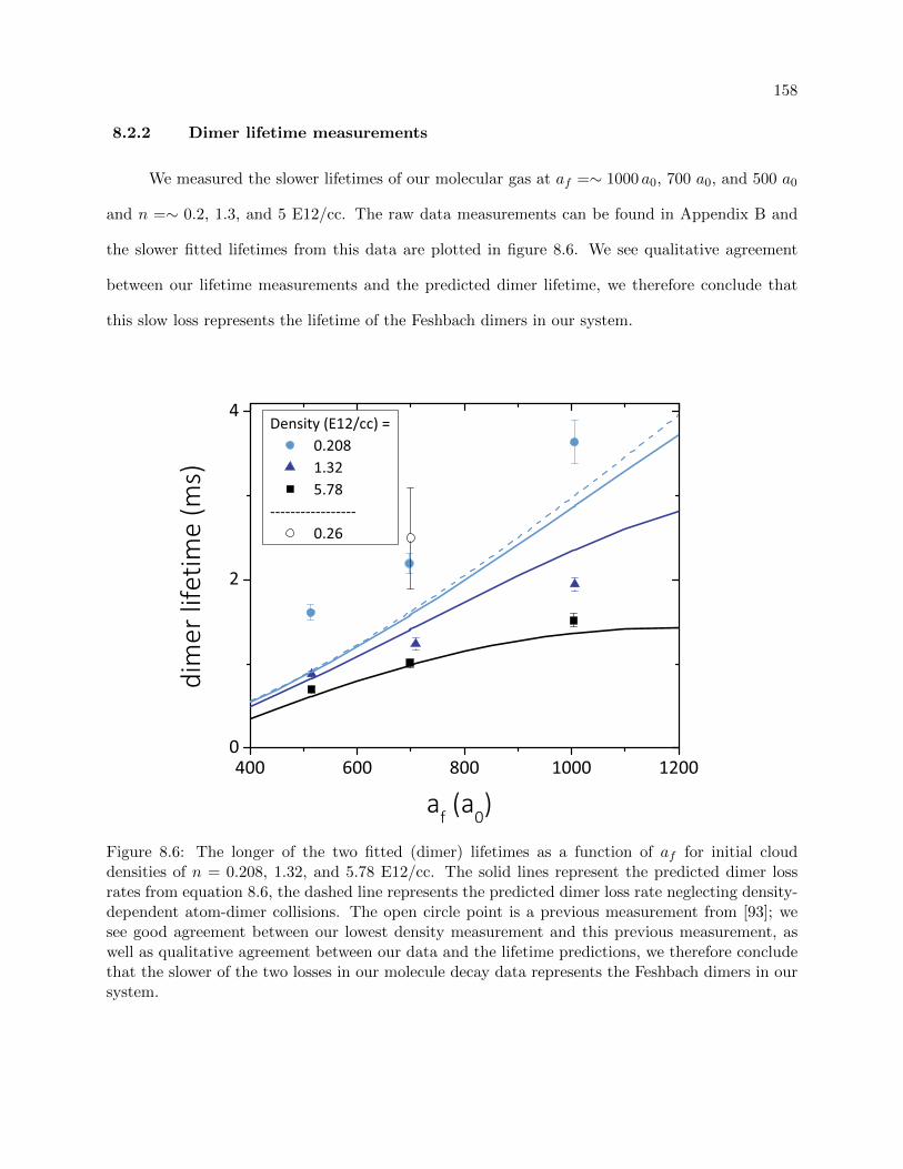
158

8.2.2 Dimer lifetime measurements

We measured the slower lifetimes of our molecular gas at af =∼ 1000 a0, 700 a0, and 500 a0

and n =∼ 0.2, 1.3, and 5 E12/cc. The raw data measurements can be found in Appendix B and

the slower fitted lifetimes from this data are plotted in figure 8.6. We see qualitative agreement

between our lifetime measurements and the predicted dimer lifetime, we therefore conclude that

this slow loss represents the lifetime of the Feshbach dimers in our system.

400 600 800 1000 12000

2

4

af (a0)

dim

er li

fetim

e (m

s)

Density (E12/cc) = 0.208 1.32 5.78

----------------- 0.26

Figure 8.6: The longer of the two fitted (dimer) lifetimes as a function of af for initial clouddensities of n = 0.208, 1.32, and 5.78 E12/cc. The solid lines represent the predicted dimer lossrates from equation 8.6, the dashed line represents the predicted dimer loss rate neglecting density-dependent atom-dimer collisions. The open circle point is a previous measurement from [93]; wesee good agreement between our lowest density measurement and this previous measurement, aswell as qualitative agreement between our data and the lifetime predictions, we therefore concludethat the slower of the two losses in our molecule decay data represents the Feshbach dimers in oursystem.

159

8.3 Trimers: the fast decay

We now turn our attention to the faster of the two decays seen our molecule decay. This

decay was previously seen to be independent of both af and n. We suspect this may be evidence

of Efimov trimers in our system.

8.3.1 Trimer lifetime prediction

Because there are in theory an infinite number of Efimov states, we must use process of

elimination to narrow down our focus to the relevant states. In our case, the second-excited and

all higher states (3, 4, 5...) have already merged with the Feshbach dimer state at the scattering

lengths we are studying, and therefore no longer exist. Only the first-excited and ground Efimov

state exist in the range we study. To understand the likely population of each of these states, we

must examine the energies of these states, E(p)T , where p designates the Efimov state, (p = 0, 1, 2...).

These energies were calculated (by Jose P. D’Incao) by solving the three-body problem in the

adiabatic hyperspherical representation [43, 8], and are plotted in figure 8.7. On resonance, the

first-excited state’s energy is only 600 Hz apart from the Feshbach state, while the Efimov ground

state’s energy is on the order of a few hundred kHz (∼ 330 kHz). This large resonant binding

energy means that if atoms were associating into ground state Efimov molecules during tdwell, the

process would happen very quickly, on the order of a few µs. However, this large resonant binding

energy also makes production of these molecules during the ramp away very unlikely. Ultimately

what is most relevant in our experiment is the fact that at the magnetic fields we are probing our

system, the binding energy of the ground-state Efimov molecule is too far away from the Fesbach

dimer’s energy for our microwave pulse to dissociate both.

Having eliminated the (p = 0) and (p ≥ 2) Efimov states from possibility, we now turn our

attention to the (p = 1) state. Because this state’s binding energy is so close to the dimer’s, we have

instead plotted the difference in this energy in figure 8.8. We see that these two states are always

less than 7 kHz apart. This small difference in energy means that if there were first-excited Efimov

160

156 158 160-600

-400

-200

0

Ener

gy (k

Hz)

B Field (Gauss)

Figure 8.7: The binding energies of the Feshbach molecule ED(blue solid line), the ground Efimov

molecule E(0)T (red solid line) and the first-excited Efimov molecule E

(1)T (red dashed) as a function

of magnetic field. The left most side of the plot ends at B = B0 = 155.04 G, the center of theFeshbach resonance.

trimers in our system, they would be transferred to our imaging state by the same microwave pulse

we use to transfer the Feshbach molecules. We also see that E(1)T at resonance is only a few hundred

of Hz; this is comparable to our value of En in our experimental range of densities. It is therefore

reasonable to expect the mechanism sweeping resonant atoms into shallow Feshbach dimers might

also sweep atoms into shallow first-excited Efimov trimers. If trimers were present in our system,

whether they are created during tdwell or during the ramp away from resonance is then a relevant

question. Given their small energies on resonance, it would be more likely that, much like the

dimers, they are created during the ramp away, as population on resonance, if occurring, would

161

take on the order of several ms to be substantial.

The shape of the first-excited trimer molecule depends on a. The distance between two of the

atoms is roughly equal to the separation in a Feshbach dimer, a. The distance of the third atom

however is set by Eb − E(1)T . If we treat the two closely spaced atoms are one particle (“dimer”),

the third atom can be approximated to be bound to the “dimer” by

Eb − E(1)T ≈ ~2

43ma

2T

, (8.7)

where aT is the distance between the third atom and the “dimer”. This distance is at a maximum

of 6.6 kHz at a =∼ 1000 a0, corresponding to aT ≈ 2200 a0; the third atom is therefore separated by

more than twice the other two atoms’ distance. At a low density of n = 0.2 E12/cc, the interparticle

distance (n−1/3) is safely > 10 times larger than the trimer size, however at our standard density

of n = 5 E12/cc, n−1/3 = 10.7 k a0, only five times the Efimov size. If there were Efimov trimers

in our system at this standard density then, many questions arise, such as what does it mean to

have a three-atom molecule when it is embedded in a gas with inter particle spacing comparable

to the molecular size?

The predicted lifetime of the trimers is how we analyze our system for their existence. The

width of the first-excited Efimov trimer (Γ), calculated by the same method as that to calculate

the binding energy, is plotted in figure 8.8. The lifetime of this state is then 1/(2πΓ), and is plotted

in 8.9. It does not vary appreciably over our studied range of a, being 100 µs at 500 a0 and only

∼ 130 µs at 1000 a0.

162

156 158 1600

2

4

6

8

Ener

gy/h

(kH

z)

B field (Gauss)

(EDimer - ETrimer)/h

Trimer

Figure 8.8: The difference between the Feshbach dimer and first-excited Efimov trimer binding

energies is plotted in purple. On resonance, E(1)T − Eb ∼ 600 Hz. The calculated width of the

first-excited trimer state is plotted in pink.

163

Figure 8.9: The predicted trimer lifetime as a function of a. This lifetime does not vary appreciablywithin our studied range of a, is 100 µs at 500 a0 and only ∼ 130 µs at 1000 a0, see inset.

164

0.1 1 100

50

100

150tri

mer

life

time

(s)

n (E12/cc)Figure 8.10: The faster of the two fitted lifetimes in our molecular gas plotted as a function ofdensity. The system was probed at af = 700 a0. The predicted trimer lifetime at this scatteringlength is 109 µs. Our measured lifetimes average to 114 ± 16.

8.3.2 Trimer lifetime measurements

We measured the fast lifetimes of our gas created by a tdwell = 1.5 tn on resonance and a ramp

time = 100 µs to 700 a0 for various densities, the results are plotted in figure 8.10. We see that the

fast lifetime does not vary with density within error, and averages to a value of 114 ± 16. This is

in very good agreement with the predicted first-excited Trimer lifetime of 109 µs at a = 700 a0.

8.3.3 How many trimers?

The excellent agreement between our measured fast decay and predicted trimer lifetime, as

well as the slower decay and the predicted dimer lifetimes, confirms the existence of first-excited

165

trimers in our system. We can now surmise that the fitted amplitudes of our exponential sum

represent the number of trimers and dimers in the system. Because the microwave pulse to our

imaging state works by spin-flipping only one atom in each molecule to the imaging state (fun fact:

the trimer atom that is sent to the imaging state in this case is one of the two closer-bound atoms),

A1 and A2 of equation (8.1) are the number of trimers and the number of dimers, respectively. The

number of atoms swept into the trimer state is then 3×A1 and into the dimer state 2×A2.

From figure 8.1 we can estimate the number of atoms that were swept into the respective

molecules. The initial condensate number was 82400 ± 1600. Given the fitted values of A1 and A2

then, we see that (3.46 ± 0.44)% atoms are swept into trimers, and (9.98 ± 0.33)% into dimers for

the n = 0.2 E12/cc dataset, and (7.1 ± 0.17)% into trimers and (12.06 ± 0.54)% into dimers for

the n = 1.32 E12/cc dataset. It is expected that the number of molecules created would depend

on the density, see Chapter 7 for further exploration into this idea.

Now that we are convinced that we are in fact creating molecules when we ramp away from

resonance, and these molecules are both Feshbach dimers and Efimov trimers, let us now explore

how the formation of these molecules is affected by dwell time on resonance.

Chapter 9

The oddities

9.1 Molecule lifetime measurements at short dwell times

We want to study how the system’s evolution of resonance affects molecule production. In

Chapter 7 we explored how the rate of the ramp away from resonance affected the molecule pro-

duction. We briefly saw that the molecule production was also affected by the initial density of the

system and the dwell time on resonance. We surmise that a minimum evolution on resonance is

necessary for molecular production.

For our initial experiment, we decreased tdwell from 1.5 to 0.15 tn, and, through fitting the

decay rates of the subsequent molecular cloud, hoped to extract the number of dimers and trimers

produced, A1 and A2 (see figure 9.1). This seemingly simple experiment hit a snag when we realized

that at a shorter tdwell our defining lifetimes of t1 and t2 had changed: t1 nearly doubled while t2

decreased by nearly 25%, from 1250 to 950 µs.

167

0 200 400 600 800 1000 12000

1k

2k

3k

4k

5k

6k

N = A1*e-t/t1 + A2*e

-t/t2

A1 = 3770(650) 4120(110)t1 = 194(32) 211(11)A2 = 1700(690) 1320(110)t2 = 950(380) 1250 fixed

hold time ( s)

mol

ecul

e nu

mbe

r

14 Sep 2016n: 1.32 E12/ccramp: 10-22.5-100 us / 0.15 tnfield: 159.2 / 699 a0RF: c (10-30-10us)

9dBm, 300 kHz, yes N: 76900 +/- 3700

Figure 9.1: The number of molecules in a n = 1.32 E12/cc system, as a function of hold time ataf = 700 a0. The molecules are generated after a tdwell = 0.15 tn on resonance and a ramp time= 100 µs to af . The data are fit with a sum of two exponentials with all fit parameters free (red)and fixing the dimer lifetime, t2 (blue, behind red) to the predicted value based on the density andaf , see equation (8.6). We see that the dimer lifetime fits to a 25% faster decay when allowed tofloat. The trimer lifetime repeatedly fits to around 200 µs, about double its expected value. Theabbreviated legend in the upper right is explained in Appendix A.

168

9.2 Dimers: the slow decay

To study how exactly tdwell affects the fitted molecular lifetimes, we took molecular decay

data of an intermediate density (n = 1.3 E12/cc) cloud at af = 700 a0 for various values of tdwell,

see Appendix C for the raw data. Due to the perceived decrease in dimer lifetimes and increase

in trimer lifetimes, our fitting function at many times had difficulty discerning two lifetimes. To

simplify matters we fixed t1 to 100 µs and have plotted the resulting fits of t2 in figure 9.2. When

tdwell ≥ 0.9 tn, t2 fits to its predicted value of 1240 µs. For tdwell ≤ 0.5 tn, we find that t2 is not

only shorter but also seems to change with tdwell.

Figure 9.2 shows that at low values (< 0.5 tn) of tdwell the fitted value of t2 does not depend

on ramp out. However, in figure 9.3 we see that ramp rate does become important near the critical

value of tdwell ∼ 1 tn. This could be due to incorrect definition of tdwell, and therefore the real,

actual resonant evolution time that the experiment cares about is changing as we vary ramp out

near the critical value.

The molecule lifetime’s perceived dependence on tdwell is very unexpected and suspicious. To

test our sanity, as well as any imaging systematics, we thoroughly checked our molecular decay

while purposefully detuning our experimental set points, see figure 9.4. For all the things we

varied, we never saw appreciable change in number at critical hold times that would change the

fitted values of t1 and t2. We therefore conclude from these checks that this odd behavior we see

from short-evolved resonant clouds is real.

169

0 1 2 30

500

1000

1500

2000

50us ramp

200us ramp

t 2 (s)

tdwell (tn)

n = 1.36 E12/cc

Figure 9.2: The fitted dimer lifetime measured in n = 1.32 E12/cc (tn = 146 µs) clouds at af =700 a0 for various resonance dwell times. For these fits we fixed t1 to 100 µs. t2 fits to its expectedvalue of 1250 µs (solid line) when tdwell ≥ 0.9 tn, but fits to much shorter lifetimes for smallertdwell’s. Most of the points (black squares) are taken after a ramp time = 100 µs to af , howeverwe also measured the lifetime for a longer ramp out time of 200 µs (orange triangle) and a shorterramp time of 50 µs (blue triangle), and saw no appreciable difference in t2 behavoir.

170

Figure 9.3: The molecule number as a function of hold time at af = 700 a0 for tdwell = 1 tn after a(a) a slower ramp time of (a) 200 µs, and (b) a faster ramp time of 50 µs. The data are fit witha sum of two exponentials while fixing the trimer lifetime , t1 (green) or fixing the dimer lifetime,t2 (blue). The slower ramp out dataset fits to normal values of t1 and t2, whereas the faster rampout dataset fits either smaller values of t2 or doubled value of t1.

171

Figure 9.4: The molecule number as a function of hold time at af = 700 a0 for tdwell = 0.15 tn witha cloud of initial density n = 1.36 E12/cc. We changed various aspects of the experiment in orderto see if the data was affected: (a) varied the imaging pulse length as well the amount of incidentimaging light. (b) Held an extra second in our hybrid optical+magnetic trap before proceedingwith the resonance-jump procedure. This checks for invisible Oort clouds that could be oscillatingin our trap and later smashing into our system. We see small decrease in number after holding theextra second, most likely due to slight heating of the system, however these drop in number doesnot explain the short fitted values of t2. (c) Decreased the microwave detuning, thereby introducingmore field-sensitive atoms into the image background. (d) No tracking of the microwave frequencyas the cloud fell. This is not expected to affect the number of molecules transferred to the imagingstate as this molecule number is saturated, and the cloud does not fall so far that the detuningexceeds Eb. (e) We expanded the molecule image by delaying the time between the microwavetransfer and the imaging laser. This expansion increases the size and decreases the optical depth,thereby testing for imaging errors related to background corrections or resolution effects. (f) Themeasured sizes of the clouds with and without expansion, we see that the new clouds are 250%their original volume. From all of these test (a-f) we conclude that the strange effects we see fromour short-evolved resonant clouds are real and not an effect from experimental error.

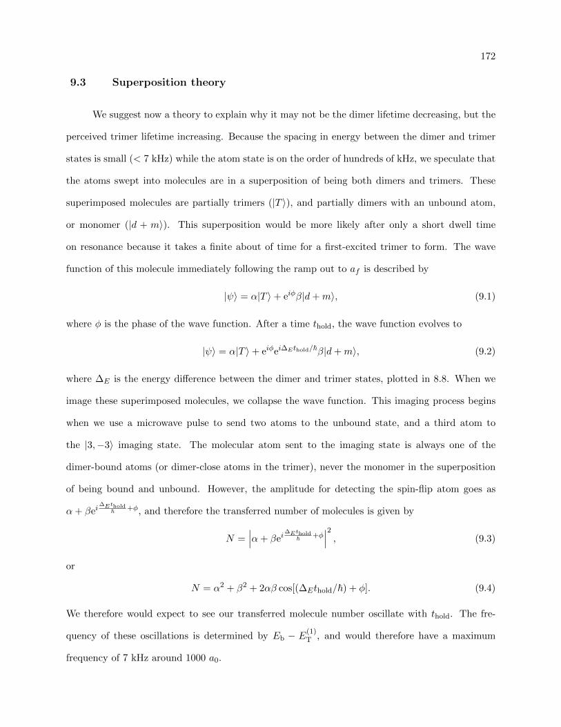
172

9.3 Superposition theory

We suggest now a theory to explain why it may not be the dimer lifetime decreasing, but the

perceived trimer lifetime increasing. Because the spacing in energy between the dimer and trimer

states is small (< 7 kHz) while the atom state is on the order of hundreds of kHz, we speculate that

the atoms swept into molecules are in a superposition of being both dimers and trimers. These

superimposed molecules are partially trimers (|T 〉), and partially dimers with an unbound atom,

or monomer (|d + m〉). This superposition would be more likely after only a short dwell time

on resonance because it takes a finite about of time for a first-excited trimer to form. The wave

function of this molecule immediately following the ramp out to af is described by

|ψ〉 = α|T 〉+ eiφβ|d+m〉, (9.1)

where φ is the phase of the wave function. After a time thold, the wave function evolves to

|ψ〉 = α|T 〉+ eiφei∆Ethold/~β|d+m〉, (9.2)

where ∆E is the energy difference between the dimer and trimer states, plotted in 8.8. When we

image these superimposed molecules, we collapse the wave function. This imaging process begins

when we use a microwave pulse to send two atoms to the unbound state, and a third atom to

the |3,−3〉 imaging state. The molecular atom sent to the imaging state is always one of the

dimer-bound atoms (or dimer-close atoms in the trimer), never the monomer in the superposition

of being bound and unbound. However, the amplitude for detecting the spin-flip atom goes as

α+ βei∆Ethold

~ +φ, and therefore the transferred number of molecules is given by

N =∣∣∣α+ βei

∆Ethold~ +φ

∣∣∣2 , (9.3)

or

N = α2 + β2 + 2αβ cos[(∆Ethold/~) + φ]. (9.4)

We therefore would expect to see our transferred molecule number oscillate with thold. The fre-

quency of these oscillations is determined by Eb − E(1)T , and would therefore have a maximum

frequency of 7 kHz around 1000 a0.

173

To search for these oscillations, we took data with very fine time steps, see figures 9.5, 9.6,

and 9.7. To the naked eye we do not see any oscillations in the molecular number. The Fourier

transform of the fit residuals of each plot (see figure 9.8) still do not see clear 7 kHz oscillations.

0 200 400 600 800

0

1k

2k

3k

hold time ( s)

16 Nov 2016n: 1.32 E12/ccramp: 10-30-100 us / 0.2 tnfield: 159.3 / 684 a0RF: c (10-30-10us)

9dBm, 300 kHz, yes N: 83900 +/- 3600

mol

ecul

e nu

mbe

r

N = A1*e-t/t

1 + A2*e-t/t

2

A1 = 2340(760) 2216(94)t1 = 228(71) 218(22)A2 = 810(800) 940(100)t2 = 1500(2400) 1250fixed

Figure 9.5: The molecule number as a function of hold time at af = 700 a0 for tdwell = 0.2 tn. Thedata are fit with a sum of two exponentials with all the parameters free (red) and fixing the dimerlifetime, t2 (blue). The residuals from the latter fit are included as blue squares. We took this datawith a high density of points in order to look for a 7 kHz oscillation in the molecular number

There are many reasons to explain why we would not see oscillations in the imaged molecular

number even if there were superimposed molecules. First, if not every trimer were a superimposed

molecule, the amplitude of the oscillations could be quite small compared to our noise. Second,

various superpositions may be out of phase with each other across the cloud, thereby washing out

the signal.

174

0 200 400 600 800 1000

0

1k

2k

3k

hold time ( s)

N = A1*e-t/t

1 + A2*e-t/t

2

A1 = 2575(62) 1991(95)t1 = 288(21) 230(25)A2 = 490(65) 1100(110)t2 = E101(--) 1250fixed

16 Nov 2016n: 1.32 E12/ccramp: 10-45-100 us / 0.3 tnfield: 159.3 / 684 a0RF: c (10-30-10us)

9dBm, 300 kHz, yes N: 83900 +/- 3600

mol

ecul

e nu

mbe

r

Figure 9.6: The molecule number as a function of hold time at af = 700 a0 for tdwell = 0.3 tn. Thedata are fit with a sum of two exponentials with all the parameters free (red) and fixing the dimerlifetime, t2 (blue). The residuals from the latter fit are included as blue squares. We took this datawith a high density of points in order to look for a 7 kHz oscillation in the molecular number

175

0 200 400 600 800 1000

0

1k

2k

3k

4k

N = A1*e-t/t

1 + A2*e-t/t

2

A1 = 1050(190) 1970(130)t1 = 69(28) 207(31)A2 = 2720(200) 1530(140)t2 = 637(67) 1250fixed

16 Nov 2016n: 1.3 E12/ccramp: 10-75-100 us / 0.5 tnfield: 159.3 / 684 a0RF: c (10-30-10us)

9dBm, 300 kHz, yes N: 83900 +/- 3600

hold time ( s)

mol

ecul

e nu

mbe

r

Figure 9.7: The molecule number as a function of hold time at af = 700 a0 for tdwell = 0.5 tn. Thedata are fit with a sum of two exponentials with all the parameters free (red) and fixing the dimerlifetime, t2 (blue). The residuals from the latter fit are included as blue squares. We took this datawith a high density of points in order to look for a 7 kHz oscillation in the molecular number

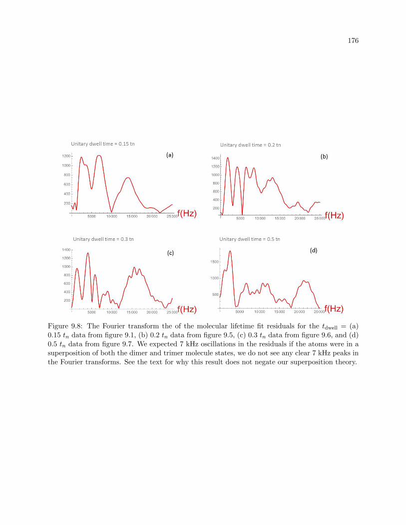
176

Figure 9.8: The Fourier transform the of the molecular lifetime fit residuals for the tdwell = (a)0.15 tn data from figure 9.1, (b) 0.2 tn data from figure 9.5, (c) 0.3 tn data from figure 9.6, and (d)0.5 tn data from figure 9.7. We expected 7 kHz oscillations in the residuals if the atoms were in asuperposition of both the dimer and trimer molecule states, we do not see any clear 7 kHz peaks inthe Fourier transforms. See the text for why this result does not negate our superposition theory.

177

9.4 Suggested analysis technique: fix dimer lifetime

We have not shown that our superposition theory is correct, however we speculate that due

to residual many-body effects there is a density-induced hybridized state with characteristics of

both dimers and trimers, whose decay would then be a combination of the two:

τH =τD + τD

2 τD τT(9.5)

Because the trimer lifetime is significantly smaller than the dimer lifetime, we can approximate

τH → 2 τT. It is worth noting that there is no immediately intuitive picture of what this hybridized

state physically is. Because there are a greater number of dimers than trimers, not all of the dimers

can be hybridized, whereas all of the trimers could. For analysis purposes, we will assume that

there are no pure trimers in the system, only dimers and our strange hybridized state. Therefore

we will assume that the lifetime of most dimers is the predicted value, which we will fix. We then

evaluate our tdwell data (in Appendix C) for t1, see figure 9.9. We see that the trimer lifetime fits

near the expected value of 100 µs when tdwell ≥ 1 tn, and fits near 200 µs from all shorter values

of tdwell. It is particularly interesting that this lifetime halves abruptly, rather than slowly. In our

current paradigm, this suggests that all the trimers in the system take a characteristic time of 1

tn to be established. The fact that the trimer lifetime for tdwell < 1 tn is always near 200 µs and

does not vary with tdwell agrees with our theory this odd behavior is due to (all) trimers being a

hybridized molecule.

From these fits we can extract A1, A2 and A3 as a function of tdwell, see figure 9.10. A2 is

the number of pure (i.e. non-hybridized) dimers, A1 (for tdwell < 1 tn) the number of hybridized

molecules, and A3 (for tdwell ≥ 1 tn) the number of pure trimers. The number of dimers peaks near

tdwell = 1.5 tn. For shorter dwell times we see that the number of hybridized molecules is greater

than the number of full dimers. This is surprising because the bound value of the trimer state on

resonance suggests that a finite time is needed to form these states, and therefore the number of

dimers would should at first be larger than A1. However, if we surmise that the mechanism to

create dimers and trimers is not the same, and that perhaps one molecule has greater production

178

value during the evolution on resonance and the other during the ramp away, then these results are

less intimidating.

0 1 20

50

100

150

200

250

300

fast

dec

ay fi

t (s)

tdwell ( s)

Figure 9.9: The fitted trimer lifetime measured in n = 1.32 E12/cc (tn = 146µs) clouds at af =700 a0 for various resonance dwell times. For these fits, we fixed t2 to 1250 µs. The black squaresare fits from the high-density-of points data, like those from figure 9.5; the blue circles are thefits from less full datasets from Appendix C and therefore have larger error bars. We see that thetrimer lifetime fits near the expected value of 100 µs when tdwell ≥ 1 tn, and fits near 200 µs from allshorter tdwell’s. It is particularly interesting that this lifetime doubles as quick as a step function,rather than slowly changing.

179

0 1 2 30

2k

4k

6k A1

A2

A3

fitte

d am

plitu

de

tdwell / tn

Figure 9.10: The fitted molecule amplitudes, A1, A2, and A3, as a function of tdwell, after analyzingthe lifetime data from Appendix C with t1 free and t2 fitted to 1241 µs. The initial condensate haddensity n = 1.36 E12/cc and was ramped to af = 700 a0 in ramp time = 100 µs. A1 (red points)is the number of hybridized molecules identified by their 200 µs lifetime, and is greater than thenumber of full dimers (A2, blue triangles) at short dwell times. A3 (black squares) is the numberof full trimers, identified by their 100 µs lifetime.

9.5 Re-examining the molecule size predictions

In Chapter 7 we examined the large role the ramp away from resonance plays in forming

the Feshbach molecules, now we wonder: does it play an equal role in producing trimers? And

hybridized molecules?

To answer these questions (or maybe develop more), we must change our interpretive per-

spective. Instead of thinking as the molecules being “created” during the dwell time on resonance

or during the ramp away, we will instead only consider the probability to form molecules, and how

180

this relates to the distance between individual atoms at resonance.

Recall from Chapter 7 the model for production of Feshbach molecules assumes that at

resonance there are molecule-like correlations with characteristic size a′. The number of atoms

swept into Feshbach molecules was then proportional to

N = 4Aa∗ · a′

(a∗ + a′)2 , (9.6)

where A is an undetermined amplitude and a∗ is a critical value of scattering length where the

ramp appears to go from diabatic to adiabatic, defined in our earlier model to be(

α~4mB

). With

our universal perspective, we assumed that a′ was proportional to 1/κn, where κn is the density

momentum defined in Chapter 2. This model fit very well to our ramp out data (evolved on

resonance for tdwell = 1.5 tn), plotted again as the dashed lines in figure 9.11(a).

Turning our attention now to 9.11(b), we see that the density dependence of the ramp out

rate becomes less defined when we evolve our system on density for a shorter amount of time. This

suggests that the effect that the ramp out rate has on forming molecules depends on how much

the system evolves on resonance. We define a new molecule size of adjusted size, s/κf , to account

for this change in density dependence. A smaller s increases the molecule number at longer ramp

times for lower density datasets and also make the initial growth in molecule number steeper for

the medium density data - see dashed lines in figure 9.11. We find that we have to include a

density dependence s for the short tdwell dataset that removes the universal scaling. We are not

fully convinced of the validity of this approach.

181

Figure 9.11: (a) The number of molecules imaged with a 300 µs Gaussian pulse as a function of rampout rate after tdwell = 1.5 tn for clouds of initial densities of n = 5.5 (blue points, tn = 57µs) and0.18 (cyan triangles, tn = 553µs) E12/cc. The dashed lines are the predicted number of moleculesto be produced assuming the molecule size is defined by 1/κn, we see good agreement with data.The solid line is the same model except the molecule size is assumed to be s/κf where s = 0.4. (b)The number of molecules imaged with a 300 µs Gaussian pulse as a function of ramp out rate aftertdwell = 0.5 tn. The dashed lines are the predicted number of molecules to be produced assumingthe molecule size is defined by 1/κn, we see very poor agreement with the data. The solid line isthe same model except the molecule size is assumed to be s/κn where s has a density dependenceof s = 0.3(n/nlow)1/3, this changes the density dependence of a′, and therefore the expected densitydependence of the ramp out data.

182

9.5.1 Changing molecule size

The difference in the ramp out data as we change dwell time on resonance suggests that the

molecule size may be changing as the cloud evolves. To study this we consider now data of the

molecular number measured as a function dwell time on resonance. The data in figure 9.12 were

taken using a 300 µs Gaussian pulse, a long pulse in which we expect the fast-decaying timers to

not be transferred to the imaging state; we see good agreement between this data and the molecule

number determined by fitting the decay for A2 (figure 9.10) and therefore conclude this number

represents only dimers.

The solid lines in figure 9.12 are the number of molecules predicted to be produced using

equation 9.6 and assuming that a′ grows linearly in time:

a′ =tdwell/ (Cgrow · tn)

(6πn)1/3. (9.7)

We see that this linear growth of a′ predicts the increase and later decrease in molecular production

very well. However, the characteristic growth rate (Cgrow) of these two datasets are in slight

disagreement, the larger density has a faster growth of 4.20(22) while the lower density dataset

grows slower, at 3.61(47). These values are barely in agreement with each other.

The value and agreement of fitted growth rates has a very large dependency on the value

a∗. For this analysis we used equation (7.5); for ramp time = 50 µs then, a∗ becomes 502 a0.

However, as we discussed at the end of chapter 7, this definition of a∗ is not without problems.

This experiment would be better then if we could remove the uncertainty of a∗ by instead controlling

it.

183

0 200 400 600 800 10000

2k

4k

6k

8k

n 5.5 0.18A 6800(150) 5640(280)C

grow 4.20(22) 3.61(0.47)

13 Jan 2016n: 5.5 0.18 E12/ccramp: 10-dwell-50 usfield: 160 GRF: G (300us)

9dBm, 400 kHz, no N: 53500 +/- --

mol

ecul

e nu

mbe

r

tdwell ( s)

Figure 9.12: The number of molecules transferred to the imaging state by a 300 µs Gaussian pulsefollowing a ramp time = 50 µs away from resonance to af = 500 a0 for condensates of initialdensities of n = 5.5 (blue points, tn = 57µs) and 0.18 (cyan triangles tn = 553µs) E12/cc. Thesolid lines are fits to the molecular number using equations 9.6 and 9.7.

9.5.2 Experiment Suggestion

We present now a suggested experiment to remove the uncertainty of a∗. By fixing a∗ we can

determine a′ (and its dependence on dwell time) through the change in produced molecule number.

The timeline is shown in figure 9.13. The experiment involves evolving the system on resonance for

various dwell times, then ramping away with a two-component ramp that is at first very fast, then

very slow. The scattering length at which the ramp rate changes is called ac, for critical value of

a. In effect, this creates a ramp where the value of a∗ is known experimentally, and is equal to ac.

The two-component ramp that is at first fast, then later slow, is essentially forcing a∗. We

184

Figure 9.13: A suggested experimental timeline for determining how a′ varies with tdwell. Afterevolving on resonance for various tdwell, ramp away at first very fast, then very slow. The criticaltime that the ramp rate switches is called ac.

can then rewrite the expected number from equation (9.6) replacing a∗ with ac. The measured

number will be a maximum when a′ = ac, and we call the dwell time that this maximum occurs

tc. Qualitative predictions for the number as a function of tdwell are shown for three different ramp

out ac values in figure 9.14(a). By plotting tc as a function of ac, we can fit the data with an

as-yet undetermined function. The inverse of the fitted function is a′(tdwell), we could know how

the molecular size changes as the cloud evolves on resonance.

185

Figure 9.14: (a) Qualitative prediction of the number of molecules produced as a function of tdwell

for ramp outs with various values of ac (corresponding the ac lines drawn in figure 9.13). Thenumber will be maximum when a′ = ac. We define the dwell time that yields maximum number astc. (b) Now plotting tc as a function of ac should yield a linear line if the growth rate on resonanceis linear. The inverse of this function yeilds a′ as a function of tdwell. We could know how themolecular size changes as the cloud evolves at unitarity.

9.5.3 Future goals

The apparatus, or machine, that produced all of the data presented in this thesis has been

dismantled. A new apparatus is currently being built in the basement of JILA. This new apparatus

will have the capability to probe the molecule clouds within the matrix of various controllable

parameters (dwell time, ramp out rate, hold time, and density) much faster, to eventually determine

how the ramp out rate and dwell time on resonance combine to sweep atoms into shallow molecules

of both dimers and trimers. This experiment will be able to create condensates of both 85Rb (like

all experiments in this thesis) and 39K, and therefore have a knob to vary the characteristic width

of the Efimov resonance, η∗.

The oddities explored in this final chapter will therefore be explored and demystified in

the near future. Much like how our scientific perspective drastically changed when we switched

from atom-loss-rate probes to molecule-production probes, I have no doubt that understanding the

evolution of a degenerate Bose gas on resonance, and how this evolution translates into propensity

to be swept into shallow molecules, will again require fresh perspectives.

Bibliography

[1] TD Lee and CN Yang. Many-body problem in quantum mechanics and quantum statisticalmechanics. Physical Review, 105(3):1119, 1957.

[2] V Efimov. Yad. fiz 12, 1080 (1970). Sov. J. Nucl. Phys, 12:589, 1971.

[3] V Efimov. Energy levels of three resonantly interacting particles. Nuclear Physics A,210(1):157–188, 1973.

[4] Eric Braaten and H-W Hammer. Universality in few-body systems with large scattering length.Physics Reports, 428(5):259–390, 2006.

[5] Javier von Stecher, Jose P DIncao, and Chris H Greene. Signatures of universal four-bodyphenomena and their relation to the efimov effect. Nature Physics, 5(6):417–421, 2009.

[6] JP DIncao, J Von Stecher, and Chris H Greene. Universal four-boson states in ultracold molec-ular gases: Resonant effects in dimer-dimer collisions. Physical review letters, 103(3):033004,2009.

[7] Scott E Pollack, Daniel Dries, and Randall G Hulet. Universality in three-and four-body boundstates of ultracold atoms. Science, 326(5960):1683–1685, 2009.

[8] Jia Wang, JP DIncao, BD Esry, and Chris H Greene. Origin of the three-body parameteruniversality in efimov physics. Physical review letters, 108(26):263001, 2012.

[9] Yujun Wang, Jose P DIncao, Brett D Esry, and CC Lin. Ultracold few-body systems. Advancesin Atomic, Molecular, and Optical Physics, 62:1–115, 2013.

[10] Swann Piatecki and Werner Krauth. Efimov-driven phase transitions of the unitary bose gas.Nature communications, 5, 2014.

[11] D Hudson Smith, Eric Braaten, Daekyoung Kang, and Lucas Platter. Two-body and three-body contacts for identical bosons near unitarity. Physical review letters, 112(11):110402,2014.

[12] M Kira. Coherent quantum depletion of an interacting atom condensate. Naturecommunications, 6, 2015.

[13] Mike H Anderson, Jason R Ensher, Michael R Matthews, Carl E Wieman, and Eric A Cornell.Observation of bose-einstein condensation in a dilute atomic vapor. science, 269(5221):198,1995.

187

[14] Kendall B Davis, M-O Mewes, Michael R Andrews, NJ Van Druten, DS Durfee, DM Kurn,and Wolfgang Ketterle. Bose-einstein condensation in a gas of sodium atoms. Physical reviewletters, 75(22):3969, 1995.

[15] Cl C Bradley, CA Sackett, JJ Tollett, and Randall G Hulet. Evidence of bose-einstein con-densation in an atomic gas with attractive interactions. Physical Review Letters, 75(9):1687,1995.

[16] Brian DeMarco and Deborah S Jin. Onset of fermi degeneracy in a trapped atomic gas. Science,285(5434):1703–1706, 1999.

[17] Christopher J Pethick and Henrik Smith. Bose-Einstein condensation in dilute gases. Cam-bridge university press, 2002.

[18] Franco Dalfovo, Stefano Giorgini, Lev P Pitaevskii, and Sandro Stringari. Theory of bose-einstein condensation in trapped gases. Reviews of Modern Physics, 71(3):463, 1999.

[19] N Bogoliubov. On the theory of superfluidity. J. Phys, 11(1):23, 1947.

[20] R. K. Pathria and Paul D. Beale. Statistical Mechanics. Academic Press, 3rd edition, 2011.

[21] Cheng Chin, Rudolf Grimm, Paul Julienne, and Eite Tiesinga. Feshbach resonances in ultracoldgases. Reviews of Modern Physics, 82(2):1225, 2010.

[22] Christopher J Foot. Atomic physics, volume 7. Oxford University Press, 2005.

[23] AJ Moerdijk, BJ Verhaar, and A Axelsson. Resonances in ultracold collisions of li 6, li 7, andna 23. Physical Review A, 51(6):4852, 1995.

[24] Neil R Claussen, SJJMF Kokkelmans, Sarah T Thompson, Elizabeth A Donley, E Hodby, andCE Wieman. Very-high-precision bound-state spectroscopy near a 85 rb feshbach resonance.Physical Review A, 67(6):060701, 2003.

[25] Tsin D Lee, Kerson Huang, and Chen N Yang. Eigenvalues and eigenfunctions of a bose systemof hard spheres and its low-temperature properties. Physical Review, 106(6):1135, 1957.

[26] PO Fedichev, MW Reynolds, and GV Shlyapnikov. Three-body recombination of ultracoldatoms to a weakly bound s level. Physical review letters, 77(14):2921, 1996.

[27] BD Esry, Chris H Greene, and James P Burke Jr. Recombination of three atoms in theultracold limit. Physical review letters, 83(9):1751, 1999.

[28] Paulo F Bedaque, Eric Braaten, and H-W Hammer. Three-body recombination in bose gaseswith large scattering length. Physical Review Letters, 85(5):908, 2000.

[29] Eric Braaten and H-W Hammer. Three-body recombination into deep bound states in a bosegas with large scattering length. Physical review letters, 87(16):160407, 2001.

[30] Tino Weber, Jens Herbig, Michael Mark, Hanns-Christoph Nagerl, and Rudolf Grimm. Three-body recombination at large scattering lengths in an ultracold atomic gas. Physical reviewletters, 91(12):123201, 2003.

188

[31] SB Papp, JM Pino, RJ Wild, S Ronen, Carl E Wieman, Deborah S Jin, and Eric A Cornell.Bragg spectroscopy of a strongly interacting rb 85 bose-einstein condensate. Physical reviewletters, 101(13):135301, 2008.

[32] Robert P Smith, Robert LD Campbell, Naaman Tammuz, and Zoran Hadzibabic. Effectsof interactions on the critical temperature of a trapped bose gas. Physical review letters,106(25):250403, 2011.

[33] Nir Navon, Swann Piatecki, Kenneth Gunter, Benno Rem, Trong Canh Nguyen, FredericChevy, Werner Krauth, and Christophe Salomon. Dynamics and thermodynamics of the low-temperature strongly interacting bose gas. Physical review letters, 107(13):135301, 2011.

[34] RJ Wild, P Makotyn, JM Pino, EA Cornell, and DS Jin. Measurements of tan’s contact in anatomic bose-einstein condensate. Physical review letters, 108(14):145305, 2012.

[35] Philip Makotyn, Catherine E Klauss, David L Goldberger, EA Cornell, and Deborah S Jin.Universal dynamics of a degenerate unitary bose gas. Nature Physics, 10(2):116–119, 2014.

[36] Philip Makotyn. Experimental studies of a degenerate unitary Bose gas. PhD thesis, Universityof Colorado at Boulder, 2014.

[37] BS Rem, AT Grier, I Ferrier-Barbut, U Eismann, T Langen, N Navon, L Khaykovich,F Werner, DS Petrov, F Chevy, et al. Lifetime of the bose gas with resonant interactions.Physical review letters, 110(16):163202, 2013.

[38] Richard J Fletcher, Alexander L Gaunt, Nir Navon, Robert P Smith, and Zoran Hadzibabic.Stability of a unitary bose gas. Physical review letters, 111(12):125303, 2013.

[39] Ulrich Eismann, Lev Khaykovich, Sebastien Laurent, Igor Ferrier-Barbut, Benno S Rem, An-drew T Grier, Marion Delehaye, Frederic Chevy, Christophe Salomon, Li-Chung Ha, et al.Universal loss dynamics in a unitary bose gas. Physical Review X, 6(2):021025, 2016.

[40] Richard J. Fletcher, Raphael Lopes, Jay Man, Nir Navon, Robert P. Smith, Martin W. Zwier-lein, and Zoran Hadzibabic. Two- and three-body contacts in the unitary bose gas. Science,355(6323):377–380, 2017.

[41] JM Diederix, TCF Van Heijst, and HTC Stoof. Ground state of a resonantly interacting bosegas. Physical Review A, 84(3):033618, 2011.

[42] Xiao Yin and Leo Radzihovsky. Quench dynamics of a strongly interacting resonant bose gas.Phys. Rev. A, 88:063611, Dec 2013.

[43] AG Sykes, JP Corson, JP D’Incao, AP Koller, CH Greene, AM Rey, KRA Hazzard, andJL Bohn. Quenching to unitarity: Quantum dynamics in a three-dimensional bose gas. PhysicalReview A, 89(2):021601, 2014.

[44] A. Rancon and K. Levin. Equilibrating dynamics in quenched bose gases: Characterizingmultiple time regimes. Phys. Rev. A, 90:021602, Aug 2014.

[45] Sebastien Laurent, Xavier Leyronas, and Frederic Chevy. Momentum distribution of a diluteunitary bose gas with three-body losses. Physical review letters, 113(22):220601, 2014.

189

[46] Maurizio Rossi, Luca Salasnich, Francesco Ancilotto, and Flavio Toigo. Monte carlo simula-tions of the unitary bose gas. Physical Review A, 89(4):041602, 2014.

[47] John P Corson and John L Bohn. Bound-state signatures in quenched bose-einstein conden-sates. Physical Review A, 91(1):013616, 2015.

[48] Shao-Jian Jiang, Jeff Maki, and Fei Zhou. Long-lived universal resonant bose gases. PhysicalReview A, 93(4):043605, 2016.

[49] Pascal Naidon and Shimpei Endo. Efimov physics: a review. Reports on Progress in Physics,80(5):056001, 2017.

[50] Eric Braaten and H-W Hammer. Efimov physics in cold atoms. Annals of Physics, 322(1):120–163, 2007.

[51] T Kraemer, M Mark, P Waldburger, JG Danzl, C Chin, B Engeser, AD Lange, K Pilch,A Jaakkola, H-C Nagerl, et al. Evidence for efimov quantum states in an ultracold gas ofcaesium atoms. Nature, 440(7082):315–318, 2006.

[52] Matteo Zaccanti, Benjamin Deissler, Chiara D’Errico, Marco Fattori, Mattia Jona-Lasinio,Stefan Muller, Giacomo Roati, Massimo Inguscio, and Giovanni Modugno. Observation of anefimov spectrum in an atomic system. Nature Physics, 5(8):586–591, 2009.

[53] M Berninger, A Zenesini, B Huang, W Harm, H-C Nagerl, F Ferlaino, R Grimm, PS Julienne,and JM Hutson. Universality of the three-body parameter for efimov states in ultracold cesium.Physical review letters, 107(12):120401, 2011.

[54] Noam Gross, Zav Shotan, Servaas Kokkelmans, and Lev Khaykovich. Nuclear-spin-independent short-range three-body physics in ultracold atoms. Physical review letters,105(10):103203, 2010.

[55] JH Huckans, JR Williams, EL Hazlett, RW Stites, and KM O’Hara. Three-body recombi-nation in a three-state fermi gas with widely tunable interactions. Physical review letters,102(16):165302, 2009.

[56] G Barontini, C Weber, F Rabatti, J Catani, G Thalhammer, M Inguscio, and F Minardi.Observation of heteronuclear atomic efimov resonances. Physical review letters, 103(4):043201,2009.

[57] S Knoop, F Ferlaino, M Mark, M Berninger, H Schobel, H-C Nagerl, and R Grimm. Obser-vation of an efimov-like trimer resonance in ultracold atom–dimer scattering. Nature Physics,5(3):227–230, 2009.

[58] Shuta Nakajima, Munekazu Horikoshi, Takashi Mukaiyama, Pascal Naidon, and MasahitoUeda. Nonuniversal efimov atom-dimer resonances in a three-component mixture of li 6.Physical review letters, 105(2):023201, 2010.

[59] Alessandro Zenesini, Bo Huang, Martin Berninger, H-C Nagerl, Francesca Ferlaino, and RudolfGrimm. Resonant atom-dimer collisions in cesium: Testing universality at positive scatteringlengths. Physical Review A, 90(2):022704, 2014.

190

[60] Ruth S Bloom, Ming-Guang Hu, Tyler D Cumby, and Deborah S Jin. Tests of universal three-body physics in an ultracold bose-fermi mixture. Physical review letters, 111(10):105301, 2013.

[61] T Lompe, TB Ottenstein, F Serwane, K Viering, AN Wenz, G Zurn, and S Jochim. Atom-dimer scattering in a three-component fermi gas. Physical review letters, 105(10):103201,2010.

[62] Thomas Lompe, Timo B Ottenstein, Friedhelm Serwane, Andre N Wenz, Gerhard Zurn, andSelim Jochim. Radio-frequency association of efimov trimers. Science, 330(6006):940–944,2010.

[63] Olga Machtey, Zav Shotan, Noam Gross, and Lev Khaykovich. Association of efimov trimersfrom a three-atom continuum. Physical review letters, 108(21):210406, 2012.

[64] Shuta Nakajima, Munekazu Horikoshi, Takashi Mukaiyama, Pascal Naidon, and MasahitoUeda. Measurement of an efimov trimer binding energy in a three-component mixture of li 6.Physical review letters, 106(14):143201, 2011.

[65] Maksim Kunitski, Stefan Zeller, Jorg Voigtsberger, Anton Kalinin, Lothar Ph H Schmidt,Markus Schoffler, Achim Czasch, Wieland Schollkopf, Robert E Grisenti, Till Jahnke, et al.Observation of the efimov state of the helium trimer. Science, 348(6234):551–555, 2015.

[66] Paul Mestrom, Jia Wang, Chris H Greene, and Jose P D’Incao. Efimov universality forultracold atoms with positive scattering lengths. arXiv preprint arXiv:1609.02857, 2016.

[67] Tino Weber, Jens Herbig, Michael Mark, Hanns-Christoph Nagerl, and Rudolf Grimm. Bose-einstein condensation of cesium. Science, 299(5604):232–235, 2003.

[68] Esben Nielsen and JH Macek. Low-energy recombination of identical bosons by three-bodycollisions. Physical review letters, 83(8):1566, 1999.

[69] Jose P DIncao, Hiroya Suno, and Brett D Esry. Limits on universality in ultracold three-bosonrecombination. Physical review letters, 93(12):123201, 2004.

[70] Frederic Chevy and Christophe Salomon. Strongly correlated bose gases. Journal of PhysicsB: Atomic, Molecular and Optical Physics, 49(19):192001, 2016.

[71] Noam Gross, Zav Shotan, Servaas Kokkelmans, and Lev Khaykovich. Observation of uni-versality in ultracold li 7 three-body recombination. Physical review letters, 103(16):163202,2009.

[72] F Ferlaino, A Zenesini, M Berninger, B Huang, H-C Nagerl, and R Grimm. Efimov resonancesin ultracold quantum gases. Few-Body Systems, 51(2-4):113–133, 2011.

[73] Scott B Papp. Experiments with a two-species Bose-Einstein condensate utilizing widelytunable interparticle interactions. PhD thesis, University of Colorado at Boulder, 2007.

[74] Juan Manuel Pino II. Strongly interacting Bose-Einstein condensates: probes and techniques.PhD thesis, University of Colorado at Boulder, 2010.

[75] Robert Johannes Wild. Contact measurements on a strongly interacting Bose gas. PhD thesis,University of Colorado at Boulder, 2012.

191

[76] Jacob Lyman Roberts. Bose-Einstein condensates with tunable atom-atom interactions: Thefirst experiments with rubidium-85 BECs. PhD thesis, 2001.

[77] David Goldberger. Improving Imaging Resolution For In-Situ Measurements of Bose-EinsteinCondensates. B.S. Thesis, University of Colorado at Boulder, 2015.

[78] G Reinaudi, T Lahaye, Z Wang, and D Guery-Odelin. Strong saturation absorption imagingof dense clouds of ultracold atoms. Optics letters, 32(21):3143–3145, 2007.

[79] Daniel A Steck. Alkali d line data. URL http://steck. us/alkalidata, 2012.

[80] Alexander L Gaunt, Tobias F Schmidutz, Igor Gotlibovych, Robert P Smith, and Zoran Hadz-ibabic. Bose-einstein condensation of atoms in a uniform potential. Physical review letters,110(20):200406, 2013.

[81] Tara E Drake. Measuring local properties of a Fermi gas in the BCS-BEC crossover. PhDthesis, University of Colorado, 2015.

[82] Victor M Perez-Garcia, Humberto Michinel, JI Cirac, M Lewenstein, and P Zoller. Dynamicsof bose-einstein condensates: Variational solutions of the gross-pitaevskii equations. PhysicalReview A, 56(2):1424, 1997.

[83] Benno S Rem. The Road to the Unitary Bose Gas. PhD thesis, Ecole Normale Superieure deParis-ENS Paris, 2013.

[84] private communication with J. P. D’Incao.

[85] Elizabeth A Donley, Neil R Claussen, Sarah T Thompson, and Carl E Wieman. Atom–moleculecoherence in a bose–einstein condensate. Nature, 417(6888):529–533, 2002.

[86] Cheng Chin and Paul S. Julienne. Radio-frequency transitions on weakly bound ultracoldmolecules. Phys. Rev. A, 71:012713, Jan 2005.

[87] Eric W. Weisstein. Blackman function, 1999.

[88] Ehud Altman and Ashvin Vishwanath. Dynamic projection on feshbach molecules: A probeof pairing and phase fluctuations. Physical review letters, 95(11):110404, 2005.

[89] P Dyke, SE Pollack, and RG Hulet. Finite-range corrections near a feshbach resonance andtheir role in the efimov effect. Physical Review A, 88(2):023625, 2013.

[90] Thorsten Koehler, Eite Tiesinga, and Paul S Julienne. Spontaneous dissociation of long-rangefeshbach molecules. Physical review letters, 94(2):020402, 2005.

[91] Eric Braaten and H-W Hammer. Enhanced dimer relaxation in an atomic and molecularbose-einstein condensate. Physical Review A, 70(4):042706, 2004.

[92] Eric Braaten and H-W Hammer. Resonant dimer relaxation in cold atoms with a large scat-tering length. Physical Review A, 75(5):052710, 2007.

[93] S. T. Thompson, E. Hodby, and C. E. Wieman. Spontaneous dissociation of 85Rb feshbachmolecules. Phys. Rev. Lett., 94:020401, Jan 2005.

Appendix A

Plot Legend

Because there are many knobs in our experiment, we have created a legend to record each

variable. the legend is printed in gray on most plots, an example is shown in figure A.1; if more than

one dataset is plotted, the legend may vary in color. The legend (in order) includes: the date the

data was taken \\ the magnetic ramp to resonance as rin - dwell time - rout / the calculated tdwell

in units of tn \\ the final B-field (in Gauss) for imaging \ af in a0 (only if the field was measured

precisely) \\ the shape of the RF pulse (sq = square, G = Gaussian, c = curved, ARP = adiabatic

rapid passage) with the duration in µs or ms \\ The set RF power in dBm, the detuning of the RF

from the atomic line shape in kHz, and whether the RF was adjusted with dwell time to track the

falling cloud (represented by binary 1 or 0) \\ the average BEC number, before resonance.

If this data has variation of any of these parameters, the name will appear in place of an

actual value. For some plots, this information may be omitted altogether.

193

Figure A.1: An example data set with a plot legend in the upper right corner.

Appendix B

Dimer lifetime fits

Here are nine datasets measuring molecular number as a function of hold time at af = 500,

700, or 1000 a0. The initial densities of the condensate before the resonance jump are about n =

0.2, 1.3, and 5 E12/cc. The molecules were created by spending tdwell = 1.5 tn on resonance before

ramping away to af at a rate of ramp time = 100 µs. We fit these times beyond 500 µs to extract

the dimer lifetime.

195

0 500 1000 1500 20000

1k

2k

3k

hold time ( s)

N = A2*e-t/t2

beyond 500us

A2 = 4030(140)t2 = 1613(93)

mol

ecul

e nu

mbe

r

4 Oct 2016n: 0.208 E12/ccramp: 10-760-100 us / 1.5 tnfield: 160.0 / 514 a0RF: c (10-30-10us)

9dBm, 400 kHz, yes N: 78100 +/- 600

Figure B.1

196

0 500 1000 1500 2000 25000

1k

2k

3k

4k

5k N = A1*e-t/t1 + A2*e

-t/t2

t1 = 124.5 (37)t2 = 2170(130)

N = A2*e-t/t2 ; beyond 500us

t2 = 2200(120)

hold time ( s)

mol

ecul

e nu

mbe

r

26 Sep 2016n: 0.208 E12/ccramp: 10-760-100 us / 1.5 tnfield: 159.2 / 698 a0RF: c (10-30-10us)

9dBm, 300 kHz, yes N: 82800 +/- 1800

Figure B.2

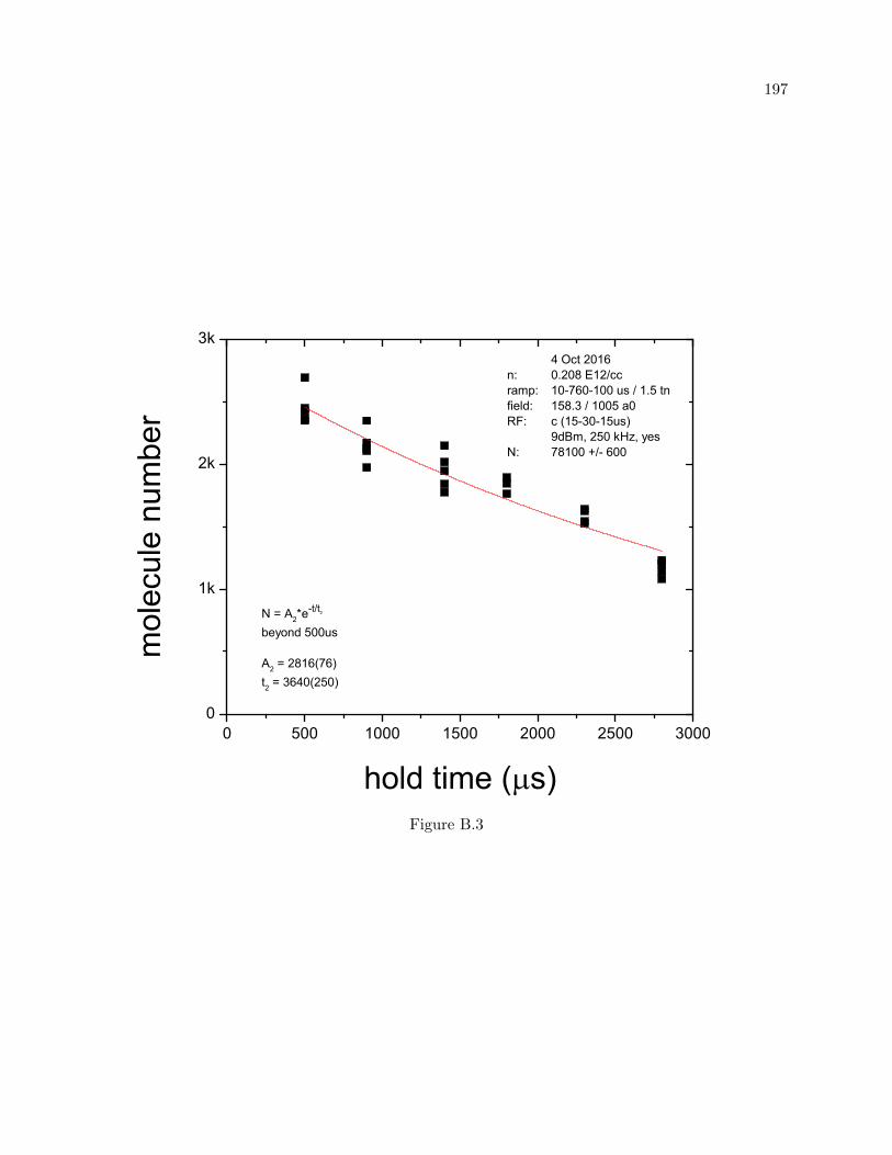
197

0 500 1000 1500 2000 2500 30000

1k

2k

3k

N = A2*e-t/t2

beyond 500us

A2 = 2816(76)t2 = 3640(250)

mol

ecul

e nu

mbe

r

hold time ( s)

4 Oct 2016n: 0.208 E12/ccramp: 10-760-100 us / 1.5 tnfield: 158.3 / 1005 a0RF: c (15-30-15us)

9dBm, 250 kHz, yes N: 78100 +/- 600

Figure B.3

198

0 500 1000 1500 20000

1k

2k

3k

hold time ( s)

mol

ecul

e nu

mbe

r

N = A2*e-t/t2

beyond 500us

A2 = 5770(210)t2 = 884(35)

4 Oct 2016n: 1.32 E12/ccramp: 10-205-100 us / 1.5 tnfield: 160.0 / 514 a0RF: c (10-30-10us)

9dBm, 400 kHz, yes N: 78100 +/- 600

Figure B.4

199

0 200 400 600 800 1000 1200 1400 1600 1800 20000

1k

2k

3k

4k

5k

6k

7k

mol

ecul

e nu

mbe

r

hold time ( s)

N = A1*e-t/t1 + A2*e

-t/t2

t1 = 97 (23) t2 = 1241(84)

N = A2*e-t/t2 beyond 500us

t2 = 1242(76)

26 Sep 2016n: 1.32 E12/ccramp: 10-384-100 us / 1.5 tnfield: 159.2 / 698 a0RF: c (10-30-10us)

9dBm, 300 kHz, yes N: 82800 +/- 1800

Figure B.5

200

500 1000 1500 2000 2500 3000500

1000

1500

2000

2500

3000

3500

mol

ecul

e nu

mbe

r

hold time ( s)

N = A2*e-t/t2

beyond 500us

A2 = 3930(100)t2 = 1948(83)

4 Oct 2016n: 1.32 E12/ccramp: 10-205-100 us / 1.5 tnfield: 158.3 / 1005 a0RF: c (15-30-15us)

9dBm, 250 kHz, yes N: 78100 +/- 600

Figure B.6

201

0 400 800 1200 16000

1k

2k

3k

hold time ( s)

mol

ecul

e nu

mbe

r

N = A2*e-t/t2

beyond 500us

A2 = 5570(260)t2 = 701(32)

4 Oct 2016n: 5.78 E12/ccramp: 10-70-100 us / 1.5 tnfield: 160.0 / 514 a0RF: c (10-30-10us)

9dBm, 400 kHz, yes N: 78100 +/- 600

med n (5.78), 1.5 tdwell, 514 a0

Figure B.7

202

0 200 400 600 800 1000 1200 1400 16000

1k

2k

3k

4k

5k

6k

7k

8k

mol

ecul

e nu

mbe

r

hold time ( s)

N = A1*e-t/t1 + A2*e

-t/t2

t1 = 129 (28) t2 = 1080(110)

N = A2*e-t/t2 beyond 500us

t2 = 1014(52)

3 Oct 2016n: 5.78 E12/ccramp: 10-70-100 us / 1.5 tnfield: 159.2 / 709 a0RF: c (10-30-10us)

9dBm, 300 kHz, yes N: 82000 +/- 2900

Figure B.8

203

0 500 1000 1500 20000

500

1k

2k

2k

3k

3k

mol

ecul

e nu

mbe

r

hold time ( s)

N = A2*e-t/t2

beyond 500us

A2 = 3570(120)t2 = 1519(77)

4 Oct 2016n: 5.78 E12/ccramp: 10-70-100 us / 1.5 tnfield: 158.3 / 1005 a0RF: c (15-30-15us)

9dBm, 250 kHz, yes N: 78100 +/- 600

Figure B.9

Appendix C

Trimer and Dimer lifetime measurements vs dwell time

Here are ten datasets measuring molecular number as a function of hold time at af = 700

a0. The initial density of the condensate before the resonance jump was either n = 1.36 E12/cc or

n = 1.32 E12/cc. The molecules were created by spending a variable amount of time on resonance,

tdwell before ramping away to af at a rate of ramp time = 100 µs (for the first eight datasets - the

last two datasets vary the ramp out rate). They were all imaged using a 50 µs curved microwave

pulse detuned 300 kHz from the atomic resonance. We attempted to fit these times with a sum of

two exponentials to extract both the dimer and trimer amplitudes. Due to the strange behavior,

we at times had to fit while fixing either t1 (green) or t2 (blue) to their expected values.

205

0 200 400 600 800 1000 1200 1400 16000

1k

2k

3k

4k

5k

hold time ( s)

mol

ecul

e nu

mbe

r

N = A1*e-t/t1 + A2*e

-t/t2

A1 = 690(200) 690(510) t1 = 100 fixed 18(18)A2 = 4300(130) 4657(63)t2 = 1560(130) 1241 fixed

30 Aug 2016n: 1.36 E12/ccramp: 10-365-100 us / 2.5 tnfield: 159.2 / 708 a0RF: c (10-30-10us)

9dBm, 300 kHz, yes N: 79000 +/- 4400

Figure C.1

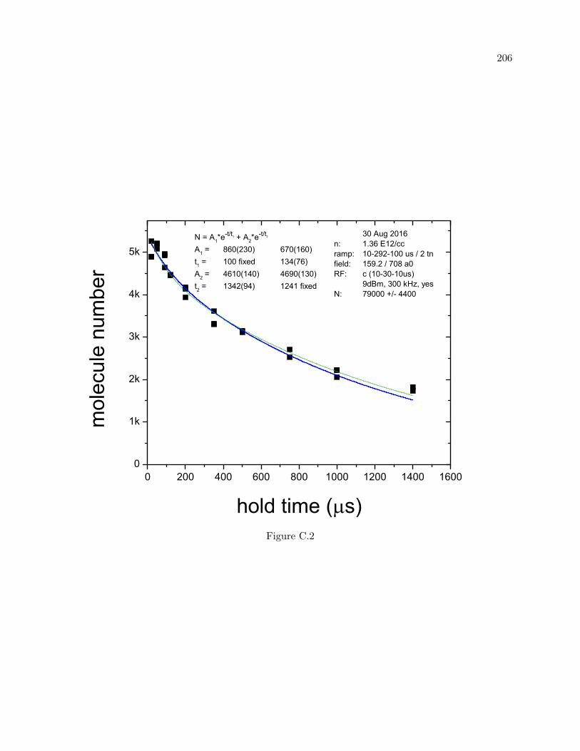
206

0 200 400 600 800 1000 1200 1400 16000

1k

2k

3k

4k

5k

mol

ecul

e nu

mbe

r

hold time ( s)

N = A1*e-t/t1 + A2*e

-t/t2

A1 = 860(230) 670(160) t1 = 100 fixed 134(76)A2 = 4610(140) 4690(130)t2 = 1342(94) 1241 fixed

30 Aug 2016n: 1.36 E12/ccramp: 10-292-100 us / 2 tnfield: 159.2 / 708 a0RF: c (10-30-10us)

9dBm, 300 kHz, yes N: 79000 +/- 4400

Figure C.2

207

0 200 400 600 800 1000 1200 1400 16000

1k

2k

3k

4k

5k

6k

7k N = A1*e-t/t1 + A2*e

-t/t2

A1 = 1680(300) 1420(220) t1 = 100 fixed 95(35)A2 = 4860(200) 5080(160)t2 = 1390(140) 1241 fixed

hold time ( s)

mol

ecul

e nu

mbe

r

18 Aug 2016n: 1.36 E12/ccramp: 10-225-100 us / 1.5 tnfield: 159.2 / 695 a0RF: c (10-30-10us)

9dBm, 300 kHz, yes N: 73900 +/- 2500

Figure C.3

208

0 200 400 600 800 1000 1200 1400 16000

1k

2k

3k

4k

5k

6k

7k

hold time ( s)

mol

ecul

e nu

mbe

r

N = A1*e-t/t1 + A2*e

-t/t2

A1 = 2310(480) 2220(420) t1 = 100 fixed 47(18)A2 = 3800(300) 4340(190)t2 = 1510(330) 1241 fixed

3 Aug 2016n: 1.36 E12/ccramp: 10-140-100 us / 1 tnfield: 159.2 / 703 a0RF: c (10-30-10us)

9dBm, 300 kHz, yes N: 73200 +/- 1000

Figure C.4

209

0 200 400 600 800 1000 1200 1400 16000

1k

2k

3k

4k

5k

6k

7k

hold time ( s)

mol

ecul

e nu

mbe

r

N = A1*e-t/t1 + A2*e

-t/t2

A1 = 2200(410) 2000(290) t1 = 100 fixed 76(25)A2 = 3940(270) 4230(193)t2 = 1410(240) 1241 fixed

29 Aug 2016n: 1.36 E12/ccramp: 10-138-100 us / 0.98 tnfield: 159.2 / 701 a0RF: c (10-30-10us)

9dBm, 300 kHz, yes N: 70500 +/- 4100

Figure C.5

210

0 500 1000 1500 2000 25000

1k

2k

3k

4k

5k

6k

7k N = A1*e-t/t1 + A2*e

-t/t2

A1 = 1670(350) 2700(260) t1 = 100 fixed 236(49)A2 = 5310(220) 4060(270)t2 = 970(72) 1241 fixed

hold time ( s)

mol

ecul

e nu

mbe

r

14 Sept 2016n: 1.32 E12/ccramp: 10-100-100 us / 0.7 tnfield: 159.2 / 699 a0RF: c (10-30-10us)

9dBm, 300 kHz, yes N: 76900 +/- 3700

Figure C.6

211

0 200 400 600 800 10000

1k

2k

3k

4k

5k

6k

mol

ecul

e nu

mbe

r

hold time ( s)

N = A1*e-t/t1 + A2*e

-t/t2

A1 = 1330(430) 3080(320) t1 = 100 fixed 233(50)A2 = 4350(320) 2510(340)t2 = 701(85) 1241 fixed

3 Aug 2016n: 1.36 E12/ccramp: 10-70-100 us / 0.5 tnfield: 159.2 / 703 a0RF: c (10-30-10us)

9dBm, 300 kHz, yes N: 73200 +/- 1000

Figure C.7

212

0 100 200 300 400 500 600 700 8000

1k

2k

3k

4k

5k

hold time ( s)

mol

ecul

e nu

mbe

r

N = A1*e-t/t1 + A2*e

-t/t2

A1 = 630(620) 3480(580) t1 = 100 fixed 260(70)A2 = 4070(520) 1210(620)t2 = 443(79) 1241 fixed

18 Aug 2016n: 1.36 E12/ccramp: 10-22.5-100 us / 0.15 tnfield: 159.2 / 695 a0RF: c (10-30-10us)

9dBm, 300 kHz, yes N: 73900 +/- 2500

Figure C.8

213

0 100 200 300 400 5000

1k

2k

3k

mol

ecul

e nu

mbe

r

hold time ( s)

N = A1*e-t/t1 + A2*e

-t/t2

A1 = 920(420) 2260(220) t1 = 100 fixed 181(65)A2 = 1970(370) 300(240)t2 = 371(85) 1241 fixed

1 Sep 2016n: 1.36 E12/ccramp: 10-0-100 us / 0.05 tnfield: 159.2 / 707 a0RF: c (10-30-10us)

9dBm, 300 kHz, yes N: 77700 +/- 1900

Figure C.9

214

0 200 400 600 800 10000

1k

2k

3k

4k

5k

N = A1*e-t/t1 + A2*e

-t/t2

A1 = 920(550) t1 = 100 fixedA2 = 3240(410) t2 = 650(130)

7 Sep 2016n: 1.32 E12/ccramp: 10-12-200 us / 0.25 tnfield: 159.2 / 702 a0RF: c (10-30-10us)

9dBm, 300 kHz, yes N: 76100 +/- 2200

hold time ( s)

mol

ecul

e nu

mbe

r

Figure C.10: rout = 200 µs

215

0 100 200 300 400 5000

1k

2k

3k N = A1*e-t/t1 + A

2*e-t/t2

A1 = 1080(660)

t1 = 100 fixed

A2 = 1760(440)

t2 = 490(200)

hold time ( s)

mol

ecul

e nu

mbe

r

7 Sep 2016n: 1.32 E12/ccramp: 10-25-50 us / 0.2 tnfield: 159.2 / 702 a0RF: c (10-30-10us)

9dBm, 300 kHz, yes N: 76100 +/- 2200

Figure C.11: rout = 50 µs

Appendix D

More molecule lifetime measurements

In this appendix we present more molecule lifetime measurements. All of these measurements

were imaged using a 50 µs curved microwave pulse detuned 300 kHz from the atomic resonance.

We attempted to fit these times with a sum of two exponentials to extract both the dimer and

trimer amplitudes.

The first six plots have an initial density of n = 0.167 E12/cc. Five datasets measure the

molecular number as a function of hold time at af = 700 a0, for the sixth dataset af = 1000 a0. The

molecules were created by spending a variable amount of time on resonance, tdwell before ramping

away to af at a rate of ramp time = 100 µs. See figure 6.21 (green triangles) for an additional

lifetime measurement with similar conditions, tdwell = 0.5 tn.

The next 6 plots are molecule lifetimes of various density, af , and tdwell values.

217

0 200 400 600 800 10000

500

1000

1500

N = A1*e-t/t1 + A2*e

-t/t2

A1 = 250(120) 661(98) t1 = 100 fixed 268(82)A2 = 1096(82) 670(110)t2 = 860(130) 1600 fixed

hold time ( s)

mol

ecul

e nu

mbe

r

2 Aug 2016n: 0.167 E12/ccramp: 10-0-100 us / 0.02 tnfield: 159.2 / 697 a0RF: c (10-30-10us)

9dBm, 300 kHz, yes N: 71700 +/- 1300

Figure D.1

218

0 500 1000 15000

1k

2k

3k

4k

hold time ( s)

mol

ecul

e nu

mbe

r

N = A1*e-t/t1 + A

2*e-t/t2

A1 = 930(270)

t1 = 139(55)

A2 = 2323(285)

t2 = 1140(180)

1 Aug 2016n: 0.167 E12/ccramp: 10-67-100 us / 0.15 tnfield: 159.2 / 699 a0RF: c (10-30-10us)

9dBm, 300 kHz, yes N: 71600 +/- 800

Figure D.2

219

0 500 1000 15000

1k

2k

3k

4k

5k

N = A1*e-t/t1 + A2*e

-t/t2

A1 = 850(190) t1 = 111(46)A2 = 3500(200)t2 = 1470(140)

29 July 2016n: 0.167 E12/ccramp: 10-246-100 us / 0.5 tnfield: 159.2 / 700 a0RF: c (10-30-10us)

9dBm, 300 kHz, yes N: 73000 +/- 1100

hold time ( s)

mol

ecul

e nu

mbe

r

Figure D.3

220

0 500 1000 1500 20000

1k

2k

3k

4k

5k

N = A1*e-t/t1 + A

2*e-t/t2

A1 = 1000(170)

t1 = 105(35)

A2 = 3830(180)

t2 = 1550(130)

hold time ( s)

mol

ecul

e nu

mbe

r

2 Aug 2016n: 0.167 E12/ccramp: 10-373-100 us / 0.75 tnfield: 159.2 / 697 a0RF: c (10-30-10us)

9dBm, 300 kHz, yes N: 71700 +/- 1300

Figure D.4

221

0 500 1000 1500 20000

1k

2k

3k

4k

5k

29 Aug 2016n: 0.167 E12/ccramp: 10-1080-100 us / 2 tnfield: 159.2 / 701 a0RF: c (10-30-10us)

9dBm, 300 kHz, yes N: 70500 +/- 4100

mol

ecul

e nu

mbe

r

hold time ( s)

N = A1*e-t/t1 + A

2*e-t/t2

A1 = 750(210) 810(270)

t1 = 100 fixed 133(88)

A2 = 3690(130) 3600(280)

t2 = 2270(270) 2410(460)

Figure D.5

222

0 500 1000 1500 2000 25000

1k

2k

3k

4k

5k

N = A1*e-t/t1 + A

2*e-t/t2

A1 = 930(150) 940(160)

t1 = 100 fixed 61(25)

A2 = 3358(95) 3460(110)

t2 = 3550(380) 3310(360)

4 Aug 2016n: 0.167 E12/ccramp: 10-510-100 us / 1 tnfield: 158.3 / 999 a0RF: c (15-30-15us)

9dBm, 250 kHz, yes N: 75000 +/- 2400

mol

ecul

e nu

mbe

r

hold time ( s)

Figure D.6: af = 1000 a0

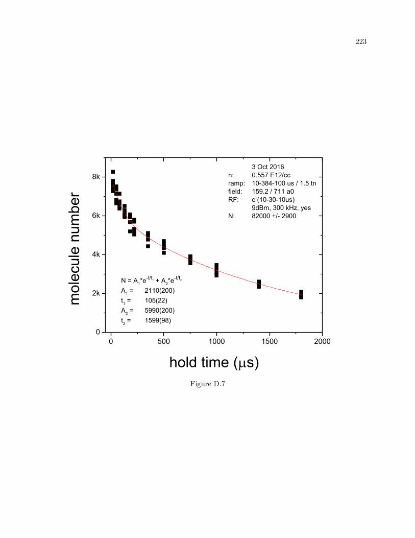
223

0 500 1000 1500 20000

2k

4k

6k

8k

N = A1*e-t/t1 + A2*e

-t/t2

A1 = 2110(200)t1 = 105(22)A2 = 5990(200)t2 = 1599(98)

3 Oct 2016n: 0.557 E12/ccramp: 10-384-100 us / 1.5 tnfield: 159.2 / 711 a0RF: c (10-30-10us)

9dBm, 300 kHz, yes N: 82000 +/- 2900

hold time ( s)

mol

ecul

e nu

mbe

r

Figure D.7

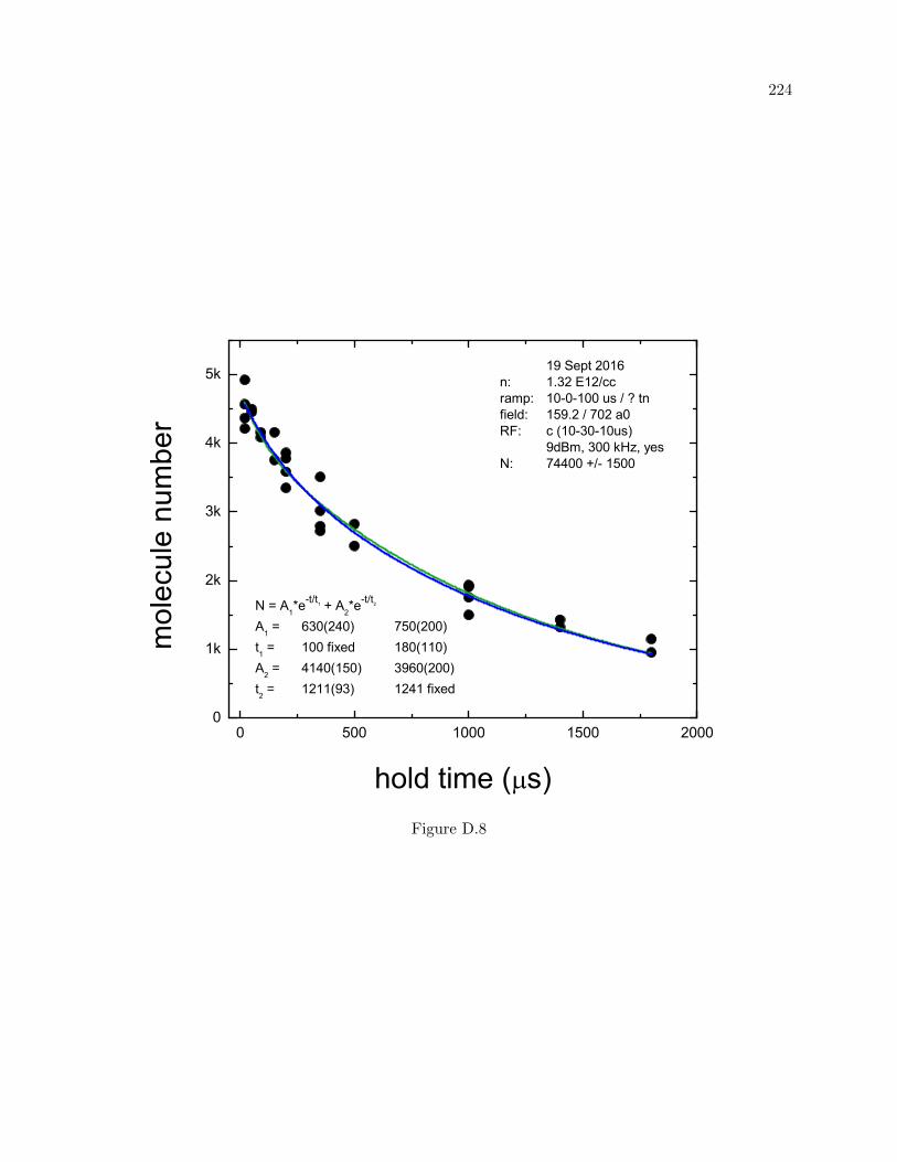
224

0 500 1000 1500 20000

1k

2k

3k

4k

5k

N = A1*e-t/t1 + A

2*e-t/t2

A1 = 630(240) 750(200)

t1 = 100 fixed 180(110)

A2 = 4140(150) 3960(200)

t2 = 1211(93) 1241 fixed

hold time ( s)

mol

ecul

e nu

mbe

r

19 Sept 2016n: 1.32 E12/ccramp: 10-0-100 us / ? tnfield: 159.2 / 702 a0RF: c (10-30-10us)

9dBm, 300 kHz, yes N: 74400 +/- 1500

Figure D.8

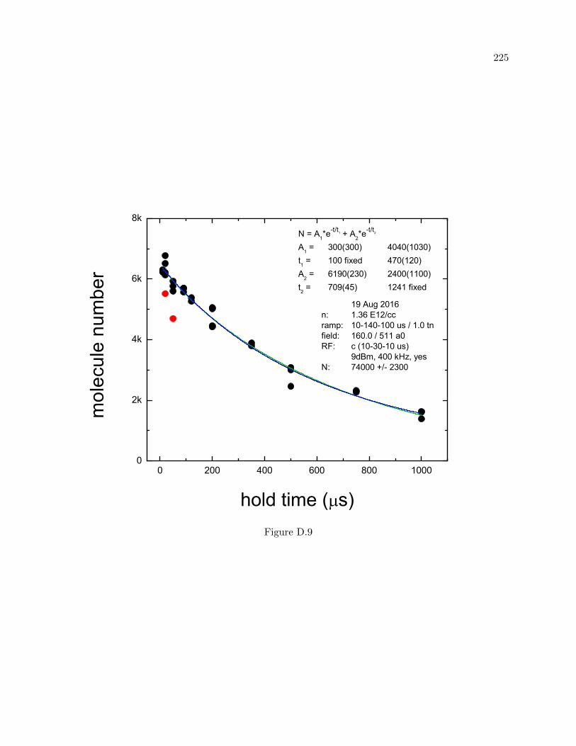
225

0 200 400 600 800 10000

2k

4k

6k

8k

hold time ( s)

mol

ecul

e nu

mbe

r

N = A1*e-t/t1 + A

2*e-t/t2

A1 = 300(300) 4040(1030)

t1 = 100 fixed 470(120)

A2 = 6190(230) 2400(1100)

t2 = 709(45) 1241 fixed

19 Aug 2016n: 1.36 E12/ccramp: 10-140-100 us / 1.0 tnfield: 160.0 / 511 a0RF: c (10-30-10 us)

9dBm, 400 kHz, yes N: 74000 +/- 2300

Figure D.9

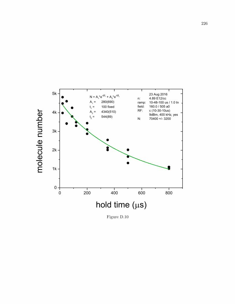
226

0 200 400 600 8000

1k

2k

3k

4k

5kN = A1*e

-t/t1 + A2*e-t/t2

A1 = 280(690)t1 = 100 fixedA2 = 4340(510)t2 = 544(89)

mol

ecul

e nu

mbe

r

hold time ( s)

23 Aug 2016n: 4.89 E12/ccramp: 10-48-100 us / 1.0 tnfield: 160.0 / 505 a0RF: c (10-30-10us)

9dBm, 400 kHz, yes N: 70400 +/- 3200

Figure D.10

227

0 200 400 600 800 10000

1k

2k

3k

4k

5k

N = A1*e-t/t1 + A2*e

-t/t2

A1 = 2400(1200)t1 = 159(89)A2 = 2100(1200)t2 = 1050(780)

mol

ecul

e nu

mbe

r

hold time ( s)

23 Aug 2016n: 4.89 E12/ccramp: 10-48-100 us / 1.0 tnfield: 159.2 / 686 a0RF: c (10-30-10us)

9dBm, 300 kHz, yes N: 70400 +/- 3200

Figure D.11

228

0 200 400 600 800 1000 1200 14000

1k

2k

3k

4k

mol

ecul

e nu

mbe

r

hold time ( s)

N = A1*e-t/t1 + A

2*e-t/t2

A1 = 1470(270)

t1 = 85(34)

A2 = 2720(270)

t2 = 1300(230)

23 Aug 2016n: 4.89 E12/ccramp: 10-48-100 us / 1.0 tnfield: 158.4 / 984 a0RF: c (15-30-15us)

9dBm, 250 kHz, yes N: 70400 +/- 3200

Figure D.12

Appendix E

Molecule lifetime measurements with square microwave pulses

Here are the remaining molecule lifetime measurements obtained using a square microwave

pulse. As the original data were contaminated by background atoms, these data were analyzed

using either the atom stripes (“stripe fit”) or atom subtraction with frequency tracking methods

(“sub constant”), see chapter 6 for more details. Additional data that fit this category can be find

in figures 6.12, 6.14, and 6.21

230

0 500 1000 1500 20000

1k

2k

3k

4k

5kN = A

1*e-t/t1 + A

2*e-t/t2 + y

0

y0 = 1413

A1 = 0(300)

t1 = 100 (fixed)

A2 = 3250(210)

t2 = 632(61)

atom offset: 72000 x 91.8% x 2% = 1413

mol

ecul

e nu

mbe

r

hold time ( s)

10 May 2016n: 0.18 E12/ccramp: 10-67-100 us / 0.15 tnfield: 159.2 / 699 a0RF: sq (50 us)

9dBm, 300 kHz, yes N: 72000 +/- 1600 sub constant

Figure E.1

231

0 500 1000 1500 20000

1k

2k

3k

4k

5k

6k

7k

hold time ( s)

mol

ecul

e nu

mbe

r

N = A1*e-t/t1 + A2*e

-t/t2 + y0

y0 = 1245A1 = 470(400) t1 = 100 (fixed) A2 = 4790(270) t2 = 826(83)

atom offset: 72000 x 86.5% x 2% = 1245

10 May 2016n: 0.18 E12/ccramp: 10-127.5-100 us / 0.25 tnfield: 159.2 / 699 a0RF: sq (50 us)

9dBm, 300 kHz, yes N: 72000 +/- 1600 sub constant

Figure E.2

232

0 500 1000 1500 20000

2k

4k

6k

8k

N = A1*e-t/t1 + A

2*e-t/t2 + y

0

y0 = 1071

A1 = 1240(230)

t1 = 74(33)

A2 = 4470(200)

t2 = 1220(100)

mol

ecul

e nu

mbe

r

hold time ( s)

9 May 2016n: 0.18 E12/ccramp: 10-246-100 us / 0.5 tnfield: 159.2 / 706 a0RF: sq (50 us)

9dBm, 300 kHz, yes N: 71300 +/- 2200

sub constant

atom offset: 71300 x 75.1% x 2% = 1071

Figure E.3

233

0 500 1000 1500 20000

2k

4k

6k

8kN = A

1*e-t/t1 + A

2*e-t/t2 + y

0

y0 = 724

A1 = 700(330)

t1 = 100 (fixed)

A2 = 4810(210)

t2 = 1220(99)

3 May 2016n: 0.18 E12/ccramp: 10-510-100 us / 1 tnfield: 159.6 / 590 a0RF: sq (50 us)

9dBm, 350 kHz, yes N: 73600 +/- 1240 sub constant

mol

ecul

e nu

mbe

r

hold time ( s)

Figure E.4: af = 590 a0.

234

0 500 1000 1500 2000 2500 3000

2k

4k

6k

8k

N = A1*e-t/t1 + A

2*e-t/t2 + y

0

y0 = 1150 1150

A1 = 1480(340) 1420(300)

t1 = 65(34) 100 (fixed)

A2 = 4860(220) 4730(180)

t2 = 2350(220) 2460(220)

2 May 2016n: 0.18 E12/ccramp: 10-510-100 us /1 tnfield: 158.7 / 842 a0RF: sq (50 us)

9dBm, 245 kHz, yes N: 75700 +/- 2100 sub constant

mol

ecul

e nu

mbe

r

hold time ( s)

Figure E.5: af = 840 a0.

235

0 500 1000 1500 2000 2500 30000.0

2.0k

4.0k

6.0k

8.0k

m

olec

ule

num

ber

hold time ( s)

26 April 2016n: 5.5 E12/ccramp: 10-108-100 us / 2 tnfield: 159.2 / 691 a0RF: sq (50 us)

9dBm, 300 kHz, yes N: 78000 +/- 1200 sub constant

N = A1*e-t/t1 + A2*e

-t/t2 + y0

y0 = 725A1 = 3240(380)t1 = 167 (34) A2 = 3970(410) t2 = 1340(160)

Figure E.6

236

0 500 1000 1500 20000

2k

4k

6k

hold time ( s)

N = A1*e-t/t1 + A2*e

-t/t2 (y0 pre sub)A1 = 720(390) 1790(350)t1 = 90 (110) 47(19) A2 = 5140(420) 5090(210)t2 = 1520(180) 1640(130)

25 April 2016n: 0.18 E12/ccramp: 10-510-100 us / 1 tnfield: 159.2 / 689 a0RF: sq (50 us)

9dBm, 300 kHz, yes N: 75600 +/- 1700 sub constant

stripes fit

mol

ecul

e nu

mbe

r

Figure E.7

237

0 1000 2000 3000 40000

2k

4k

6k

8k

N = A1*e-t/t1 + A2*e

-t/t2 (y0 pre sub)A1 = 1990(510) 4900(3700)t1 = 44 (21) 33(19) A2 = 5140(200) 6390(210)t2 = 2780(250) 3120(280)

25 April 2016n: 0.18 E12/ccramp: 10-510-100 us / 1 tnfield: 158.4 / 989 a0RF: sq (50 us)

9dBm, 200 kHz, yes N: 75600 +/- 1700 sub constant

stripes fit

hold time (us)

mol

ecul

e nu

mbe

r

Figure E.8: af = 990 a0.

238

0 500 1000 1500 2000 25000

2k

4k

6k

hold time ( s)

N = A1*e-t/t1 + A2*e

-t/t2 (y0 pre sub)A1 = 2360(1210) 6000(20000)t1 = 27 (19) 11(24) A2 = 4500(190) 4000(160)t2 = 2780(340) 2100(230)

25 April 2016n: 0.18 E12/ccramp: 10-510-100 us / 1 tnfield: 158.3 / 1005 a0RF: sq (50 us)

9dBm, 200 kHz, yes N: 78500 +/- 1500 sub constant

stripes fit

mol

ecul

e nu

mbe

r

Figure E.9: af = 1005 a0.

239

0 500 1000 1500 20000

2k

4k

6k

N = A1*e-t/t1 + A2*e

-t/t2 (y0 pre sub)A1 = 2530(3000) 1460(520)t1 = 350 (430) 170(93) A2 = 3870(3160) 5470(560)t2 = 2100(2110) 1300(160)

25 April 2016n: 0.18 E12/ccramp: 10-510-100 us / 1 tnfield: 160.1 / 502 a0RF: sq (50 us)

9dBm, 400 kHz, yes N: 78500 +/- 1500 sub constant

stripes fit

hold time (us)

mol

ecul

e nu

mbe

r

Figure E.10: af = 1005 a0.

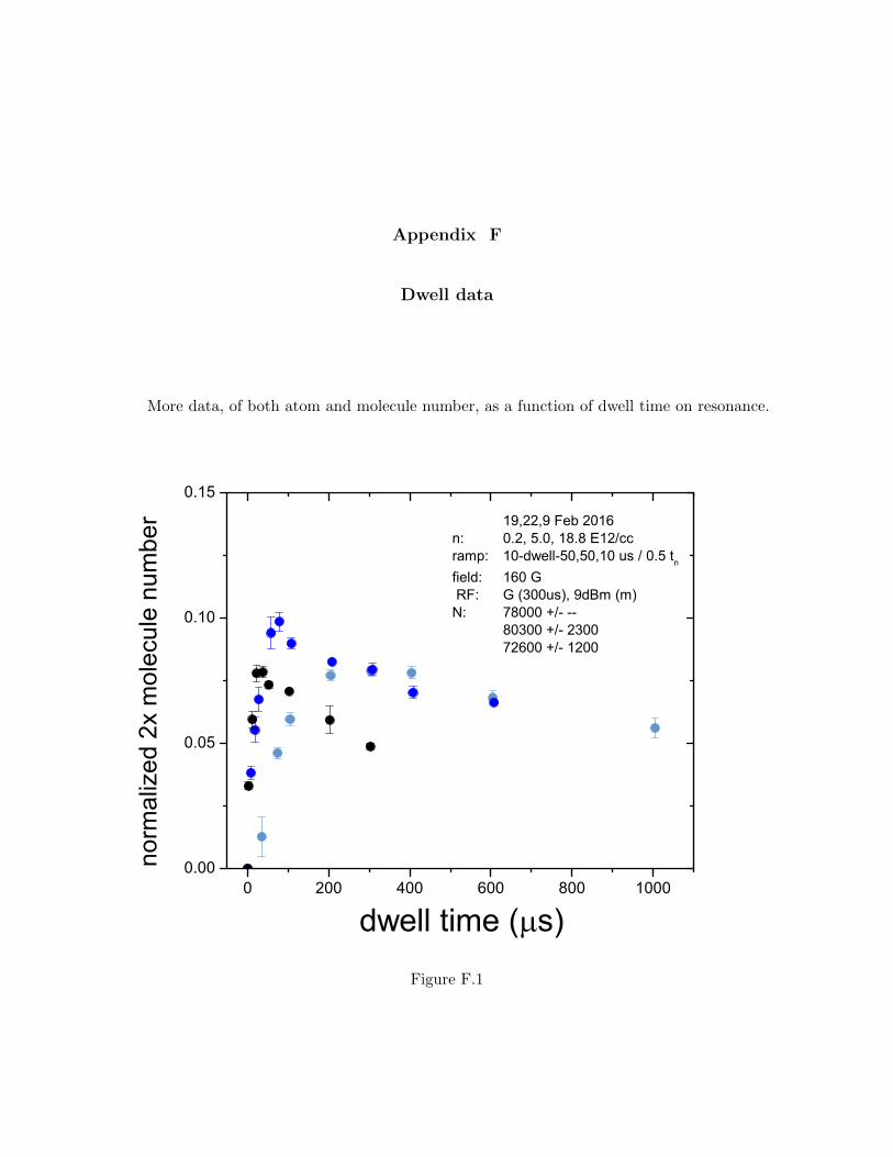
Appendix F

Dwell data

More data, of both atom and molecule number, as a function of dwell time on resonance.

0 200 400 600 800 10000.00

0.05

0.10

0.15

dwell time ( s)

19,22,9 Feb 2016n: 0.2, 5.0, 18.8 E12/ccramp: 10-dwell-50,50,10 us / 0.5 tn

field: 160 G RF: G (300us), 9dBm (m)N: 78000 +/- --

80300 +/- 230072600 +/- 1200

norm

aliz

ed 2

x m

olec

ule

num

ber

Figure F.1

241

0 1 2 3 40.0

0.2

0.4

0.6

0.8

1.0

tdwell / tn

19,22,9 Feb 2016n: 0.2, 5.0, 18.8 E12/ccramp: 10-dwell-50,50,10 us / 0.5 tn

field: 160 G RF: ARP (2ms), 9dBmN: 78000 +/- --

80300 +/- 230072600 +/- 1200

norm

aliz

ed a

tom

num

ber

Figure F.2

Appendix G

Rampout data

More molecule ramp out data.

0 200 400 600 8000

1k

2k

3k

4k

26 Oct 2016n: 0.208 E12/ccramp: 10-dwell-ramp us / 1.5 tn 0.15tnfield: 160G / 500 a0

RF: c (10-30-10 us) 9 dBm, 350 kHz, yes

mol

ecul

e nu

mbe

r

rout ( s)Figure G.1: curved RF envelope, waited hold time = 500 µs at af before beginning RF pulse.

243

0 200 400 600 8000

2k

4k

6k

8k

25 Oct 2016n: 0.208 E12/ccramp: 10-dwell -ramp us / 1.5 t

n

field: 160G / 500 a0

RF: G (300 us) 9 dBm, 350 kHz, no

N: 86200 +/- 2700

mol

eucl

e nu

mbe

r

rout ( s)

Figure G.2

244

0 200 400 600 8000

2k

4k

6k

8k

10k

mol

eucl

e nu

mbe

r

rout ( s)

19 Oct 2016n: 0.208 E12/ccramp: 10-dwell-ramp us / 1.0 t

n

field: 160G / 504 a0

RF: G (300 us) 9 dBm, 400 kHz, no

N: 73900 +/- 4300

Figure G.3

245

0 100 200 300 4000

1k

2k

3k

4k

5k

6k

rout ( s)

mol

eucl

e nu

mbe

r

19 Oct 2016n: 5.78 E12/ccramp: 10-dwell -ramp us / 1.0 t

n

field: 160G / 504 a0

RF: G (300 us) 9 dBm, 400 kHz, no

N: 73900 +/- 4300

Figure G.4

246

0 20 40 600

1k

2k

3k

4k

5k

rout ( s)

mol

ecul

e nu

mbe

r

9 Feb 2016n: 18.8 E12/ccramp: 10-12-ramp us field: 160G / 504 a0

RF: G (300 us) 9 dBm, 300 kHz, no

N: 72600 +/- 1200

Figure G.5

Appendix H

Data reference tables

FT* = frequency tracking?

Table H.1: Molecule Rampout Data

Figure Date Density tdwell af RF envelope RF duration δ FT* BEC N σNG.1 26 Oct 0.208 0.15 500 curved 50 350 1 77600 2000G.1 26 Oct 0.208 1.5 500 curved 50 350 1 77600 2000G.2 25 Oct 0.208 1.5 500 Gaussian 300 350 0 86200 2700G.3 19 Oct 0.208 1 504 Gaussian 300 400 0 73900 4300G.4 19 Oct 5.78 1 504 Gaussian 300 400 0 73900 43006.19 8 Jun 5.5 0.5 498 square 50 400 0 70000 –6.19 7 Jun 5.5 0.5 496 Gaussian 300 400 0 78000 –G.5 9 Feb 18.8 0.5 504 Gaussian 300 300 0 72600 12007.6 13 Jan 0.18 0.5 500 Gaussian 300 400 0 53500 –7.6 13 Jan 5.5 0.5 500 Gaussian 300 400 0 53500 –

248

Table H.2: Molecule Lifetime Data

Figure Date Density tdwell dwell time rout rin af RF envelope RF duration δ BEC N σN– 2016 E12/cc tn µs µs µs a0 – µs kHz – –9.5 16 Nov 1.3 0.2 30 100 10 683.5 curved 50 (10-30-10) 300 83900 36009.6 16 Nov 1.3 0.5 75 100 10 683.5 curved 50 (10-30-10) 300 83900 36009.7 16 Nov 1.3 0.3 45 100 10 683.5 curved 50 (10-30-10) 300 83900 3600B.1 4 Oct 0.208 1.5 760 100 10 514 curved 50 (10-30-10) 400 78100 600B.3 4 Oct 0.208 1.5 760 100 10 1005 curved 60 (15-30-15) 250 78100 600B.4 4 Oct 1.32 1.5 205 100 10 514 curved 50 (10-30-10) 400 78100 600B.6 4 Oct 1.32 1.5 205 100 10 1005 curved 60 (15-30-15) 250 78100 600B.7 4 Oct 5.78 1.5 70 100 10 514 curved 50 (10-30-10) 400 78100 600B.9 4 Oct 5.78 1.5 70 100 10 1005 curved 60 (15-30-15) 250 78100 600B.8 3 Oct 5.78 1.5 70 100 10 709 curved 50 (10-30-10) 300 82000 2900D.7 3 Oct 0.557 1.5 384 100 10 711 curved 50 (10-30-10) 300 82000 2900B.2 26 Sep 0.208 1.5 760 100 10 698 curved 50 (10-30-10) 300 82800 1800B.5 26 Sep 1.32 1.5 205 100 10 698 curved 50 (10-30-10) 300 82800 1800D.8 19 Sep 1.32 0.02 0 100 550 702 curved 50 (10-30-10) 300 74400 15009.1 14 Sep 1.32 0.15 22.5 100 10 699 curved 50 (10-30-10) 300 76900 3700C.6 14 Sep 1.32 0.7 100 100 10 699 curved 50 (10-30-10) 300 76900 37009.3 12 Sep 1.36 1 121 200 10 705 curved 50 (10-30-10) 300 73700 21009.3 12 Sep 1.36 1 143.6 50 10 705 curved 50 (10-30-10) 300 73700 21009.4 8 Sep 1.36 0.15 22.5 100 10 694 curved 50 (10-30-10) 300(250) 75900 2700C.11 7 Sep 1.36 0.2 30 50 10 702 curved 50 (10-30-10) 300 76100 2200C.10 7 Sep 1.36 0.25 12 200 10 702 curved 50 (10-30-10) 300 76100 2200C.9 1 Sep 1.36 0.05 0 100 10 707 curved 50 (10-30-10) 300 77700 1900C.2 30 Aug 1.36 2 292 100 10 708 curved 50 (10-30-10) 300 79000 4400C.1 30 Aug 1.36 2.5 365 100 10 708 curved 50 (10-30-10) 300 79000 4400D.5 29 Aug 0.167 2 1080 100 10 701 curved 50 (10-30-10) 300 70500 4100C.5 29 Aug 1.36 0.98 138 100 10 701 curved 50 (10-30-10) 300 70500 4100D.12 23 Aug 4.89 1 48 100 10 984 curved 60 (15-30-15) 250 70400 3200D.11 23 Aug 4.89 1 48 100 10 686 curved 50 (10-30-10) 300 70400 3200D.10 23 Aug 4.89 1 48 100 10 505 curved 50 (10-30-10) 400 70400 3200D.9 19 Aug 1.36 1 140 100 10 511 curved 50 (10-30-10) 400 74900 23008.2 19 Aug 1.36 1 140 100 10 1006 curved 60 (15-30-15) 250 74900 2300C.3 18 Aug 1.36 1.5 225 100 10 695 curved 50 (10-30-10) 300 73900 2500C.8 18 Aug 1.36 0.15 22.5 100 10 695 curved 50 (10-30-10) 300 73900 2500D.6 4 Aug 0.167 1 510 100 10 999 curved 60 (15-3-15) 250 75000 2400C.4 3 Aug 1.36 1 140 100 10 703 curved 50 (10-30-10) 300 73200 1000C.7 3 Aug 1.36 0.5 70 100 10 703 curved 50 (10-30-10) 300 73200 1000D.4 2 Aug 0.167 0.75 373 100 10 697 curved 50 (10-30-10) 300 71700 1300D.1 2 Aug 0.167 0.02 0 100 10 697 curved 50 (10-30-10) 300 71700 1300D.2 1 Aug 0.167 0.15 67 100 10 699 curved 50 (10-30-10) 300 71600 800D.3 29 July 0.167 0.5 246 100 10 700 curved 50 (10-30-10) 300 73000 11006.21 29 July 0.167 1.5 760 100 10 700 curved 50 (10-30-10) 300 73000 1100E.3 9 May 0.18 0.5 246 100 10 706 square 50 300 71300 22006.21 9 May 0.18 1.5 756 100 10 706 square 50 300 71300 2200E.1 10 May 0.18 0.15 67 100 10 699 square 50 300 72000 1600E.2 10 May 0.18 0.25 127.5 100 10 699 square 50 300 72000 1600E.4 3 May 0.18 1 510 100 10 590 square 50 350 73600 1240E.5 2 May 0.18 1 510 100 10 842 square 50 245 75700 2060E.6 26 April 5.5 2 108 100 10 691 square 50 300 78000 1200E.7 25 April 0.18 1 510 100 10 689 square 50 300 75600 1700E.8 25 April 0.18 1 510 100 10 989 square 50 200 75600 1700E.9 20 April 0.18 1 510 100 10 1005 square 50 200 78500 1500E.10 20 April 0.18 1 510 100 10 502 square 50 400 78500 15006.14 12 April 0.18 1 510 100 10 710 square 50 300 75000 16006.12 5 April 0.18 1 510 100 10 690 square 50 300 72300 1200