W&M ScholarWorks W&M ScholarWorks

Dissertations, Theses, and Masters Projects Theses, Dissertations, & Master Projects

Spring 2016

Resolution Limits of Time-of-Flight Mass Spectrometry with Resolution Limits of Time-of-Flight Mass Spectrometry with

Pulsed Source Pulsed Source

Guangzhi Qu College of William and Mary, gqu@email.wm.edu

Follow this and additional works at: https://scholarworks.wm.edu/etd

Part of the Physics Commons

Recommended Citation Recommended Citation Qu, Guangzhi, "Resolution Limits of Time-of-Flight Mass Spectrometry with Pulsed Source" (2016). Dissertations, Theses, and Masters Projects. Paper 1477068405. http://doi.org/10.21220/S2F304

This Dissertation is brought to you for free and open access by the Theses, Dissertations, & Master Projects at W&M ScholarWorks. It has been accepted for inclusion in Dissertations, Theses, and Masters Projects by an authorized administrator of W&M ScholarWorks. For more information, please contact scholarworks@wm.edu.

Resolution Limits of Time-of-Flight Mass Spectrometry with a Pulsed Source

Guangzhi Qu

Dalian, Liaoning China

Master of Science, College of William and Mary, 2009 Bachelor of Science, University of Science and Technology of China, 2007

A Dissertation presented to the Graduate Faculty of the College of William and Mary in Candidacy for the Degree of

Doctor of Philosophy

Department of Physics

The College of William and Mary August, 2016

© Copyright by Guangzhi Qu 2016

ABSTRACT PAGE

Matrix Assisted Laser Desorption/Ionization (MALDI) is a time-of-flight

mass spectrometry commonly used to detect a wide mass range of

biomarkers. However, MALDI requires a high laser pulse energy to

create ions with a mass higher than 50,000 Daltons. That high laser

energy increases the net ion production but it also degrades the

instrument's mass resolution. This project uses a Room Temperature

Ionization Liquid (RTIL) as a liquid matrix with a self healing surface

instead of a standard crystal matrix to increase shot to shot

reproducibility, enabling a systematic study of the origin of the

resolution degradation. This study shows that the main source of the

resolution degradation is the ionic space charge which delays the

ejection of ions into the acceleration region, essentially increasing the

ionization pulse time to be as long as hundreds of nanoseconds. This

study includes simulation and experimental results to document this

effect.

i

TABLE OF CONTENTS

Acknowledgements ii

Dedications iii

List of Figures iv

Chapter 1. Introduction 1

Chapter 2. Theory 11

Chapter 3. Apparatus 29

Chapter 4. Non Linear Production Process and Limits on Resolution 44

Chapter 5. Simulation 61

Chapter 6. Conclusion 87

Bibliography 92

Vita 95

ii

ACKNOWLEDGEMENTS

First and foremost, I would like to thank my advisor, Dr. William Cooke for his endless support, patient guidance and positive outlook and perseverance throughout the research. I admire the motivational optimism and excitement he shows on physics research which always inspires me with a big smile. I am so grateful for his confidence and freedom he left to me on the research. This research would not be possible if otherwise. I would also thank Dr. Dennis Manos and Dr. Eugene Tracy contributing their brilliant suggestion and insightful questions into my research work. I have truly appreciated the group members during the years. I could not have asked for better support from such a collaborative group. I am very fortunate to make great friends over the past years. Without your tremendous support and constant companion, I would not have so much fun during these years. In addition, I would like to thank all staff members in physics department. Without their assistance, our graduate life would not be smooth. Lastly, I would like to thank both of my parents. The uncertainties of pursuing degree abroad are hard to grasp. However, their confidence and faith in me supports me to finish my degree.

iii

This Ph.D. is dedicated to my parents and my grandma

iv

LIST OF FIGURES

1.1 Mass spectra from Ciphergen PBS II 2

1.2 The number of cancer death by ACS 4

1.3 Mass spectra from an NCI leukemia serum protein 7

2.1 TOF-SIMS image of prepared IMAC-Cu chip 14

2.2 Linear time of fight mass spectrometer 16

2.3 Structures of BMIM+, PF6-, Imidazolium+ 19

2.4 Summed 100 shots spectra of copper isotopes 20

2.5 PF6- peak temporal and mass resolution 22

2.6 Conventional MALDI QC spectra 23

2.7 RTIL spectra of BMIM+ and PF6- 24

2.8 Scheme of delayed extraction 26

2.9 Conventional MALDI QC spectra in high mass range 27

3.1 Overview of vacuum chamber 31

3.2 The microchannel plate detector in Chevron mode 32

3.3 Temporal profile of ND: YAG laser pulses 35

3.4 The ionization source assembly 37

3.5 Sample holder sketch 38

3.6 Drawing of top down illumination system and stainless steel plate with a slit 39

3.7 Attenuator calibrating factor 42

3.8 Multichannel plate gain calibration 43

v

4.1 Positive ion from RTIL spectra 45

4.2 Integrated signal as function of laser intensity 46

4.3 BMIM+ spectrum at low and high laser power 47

4.4 Heatmap of 100 laser shots at 2.5MW/cm2 laser intensity 47

4.5 Heatmap of 100 laser shots at 50MW/cm2 laser intensity 48

4.6 BMIM+ single shots from figure 4.5 48

4.7 Heatmap of sorted BMIM+ peaks with integral signal 49

4.8 BMIM+ single shots from figure 4.8 50

4.9 Heatmap of figure 4.7 with picked fast and slow ions 52

4.10 Process to pick out fastest and slowest ion 52

4.11 Full width of BMIM+ in terms of total ion intensity 53

4.12 BMIM+ full width versus total signal with different detector position setup 54

4.13 Detector gain ratio calibration 56

4.14 BMIM+ peak width in term of ion production with different energy 57

4.15 BMIM+ peak width in term of ion production with different initial electric field 57

4.16 Heatmap of metal piece 59

4.17 BMIM+ and Cr+ peak width versus total ion signal 59

5.1 Time distribution of 100 ions with space charge model 63

5.2 Time distributions as ion counts increases 64

5.3 Time distributions comparison with ode45 solver and fixed

vi

time step solver 66

5.4 Time distribution comparison with and without image Charge 68

5.5 Time distributions of 40 thousands and 0.2 million ions 70

5.6 Ion oscillation near acceleration plate of 0.2 million ions 71

5.7 Simulation of BMIM+ in 3kV/cm electric field 73

5.8 Simulation and real data conversion factor 74

5.9 Compare simulation and data with high ion count 74

5.10 Simulation of Cr+ ions in 3kV/cm electric field 75

5.11 Simulation distributions with different spatial distributions 76

5.12 Simulation distributions with different launching threshold 77

5.13 Simulation distributions with different laser pulse width 78

5.14 Simulation distributions with different reservoir thickness 79

5.15 Simulation of BMIM+ in 1kV/cm electric field 80

5.16 Simulation distribution of 0.4 million BMIM+ at 50cm Detector 81

5.17 Time distribution of 0.4 million BMIM+ vs simulation 82

5.18 Simulation of BMIM+ at 10cm and 50cm detector 83

5.19 CPU and GPU architecture comparison 85

5.20 Slice model simulation of 400 thousands BMIM+ 86

5.21 Comparison between ion reservoir model and slice model 87

1

Chapter 1

Introduction

The principles of time of flight (TOF) mass spectrometry (MS) have

been established for decades [1, 2, 3]. But after the first demonstration

of a laser in 1960 by Theodore H. Maiman, the TOF-MS technique

underwent rapid development. This was particularly true after Karas,

Bachmann and Hillenkamp introduced Matrix Assisted Laser

Desorption (MALDI) in 1985 [4], which provided a soft ionization

mechanism so that time of flight mass spectrometry could detect

biomarkers in a relatively wide mass range [5]. However, in order to

see the highest mass ions, one typically uses a high laser power,

which degrades the resolution of the time of flight mass spectrometer.

Even narrow, atomic lines show a broadening at high laser powers,

which has been interpreted as being due to a wide spread of initial

velocities. Figure 1.1 displays two spectra produced by different laser

powers. The spectrum is from the Quality Control (QC) data of a

2

Leukemia study organized by John Semmes of the Eastern Virginia

Medical School. The net ion production grows as laser power

increases, but the resolution of the spectra decreases. The peaks grow

broader and shift towards later times. The resolution decrease

obscures some of the smaller biomarkers that are adjacent to

dominant peaks, such as those marked by green circles. We observe

the same phenomena in our experiments. This thesis demonstrates

that this resolution decrease is not due to velocity spread, but that the

large ion cloud creates a space charge that prevents ions from

entering the accelerating field. Thus, the broadened lines are due to a

spread of times that the ions enter the accelerating region, not a

spread of initial velocities.

Figure 1.1 Typical mass spectra at high and low laser power using a Ciphergen

PBS II instrument to analyze QC blood serum.

3

1.1 Motivation

1.1.1 Early Cancer Diagnose

Cancer has been a major social health problem over recent years in

the United States and all over the world. It is expected to soon be the

leading disease causing premature death, surpassing heart disease.

Cancer Facts & Figure 2015 (American Cancer Society) [6] estimates

annual rates in the United States of 1,658,370 newly diagnosed cancer

cases diagnosed and 589,430 cancer deaths.

Early diagnosis can be crucial in the treatment and control of cancer.

Although conventional diagnosis strategies have improved detection,

the sensitivity and specificity of these methods are still not decisive in

the early stages. In most cases, a clinician analyzes a sample tissue

from patients, using an optical microscope. But, often this biopsy

process happens in a relatively late stage. Many cancer cases are not

diagnosed and treated until abnormal cancer cells have had time to

spread out to invade the surrounding tissue. Treatment is much more

difficult once a tumor spreads from its original site. Cancer detection at

early stage, especially at a premalignant stage would likely decrease

the death rate and improve treatment strategies.

4

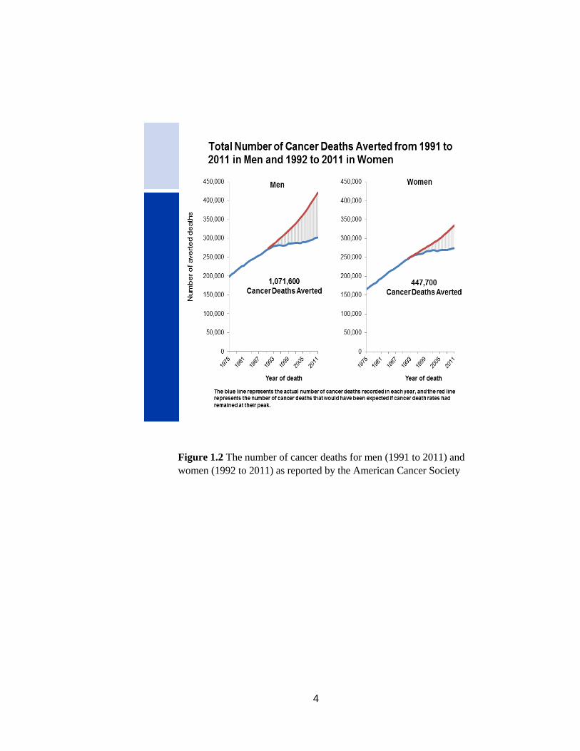
Figure 1.2 The number of cancer deaths for men (1991 to 2011) and

women (1992 to 2011) as reported by the American Cancer Society

5

1.1.2 Proteomics and Biomarkers

Although many diseases have now been determined to be the result of

defective genes, the expression of that and most other diseases

occurs when new or different proteins are produced, either by the

defective genes, or by the other disease agents. Thus, the proteins in

a person encode, in a very complex way, the current state of that

person’s health. However, there are many thousands of different

proteins in any person at any time. The study of these proteins, called

proteomics, began at the end of last century [7, 8]. Most proteins are

normal products of life, but some researchers began an attempt to

identify specific proteins that represent the presence of various

cancers [9, 10]. The Semmes group at the Eastern Virginia Medical

School (EVMS) began a series of experiments to find proteins

indicative of breast and prostate cancer in blood serum. This began

with a survey of as broad mass range of proteins as possible using

MALDI to ionize the proteins, and time-of-flight to identify their charge

to mass ratio. Due to the complexity and variability of biological

material, mass spectrometry is a powerful tool to detect and identify

proteins and peptides in a broad mass range. A protein that correlates

with the presence or absence of a disease is called a biomarker, such

6

a biomarker, if it is detected when the disease is in its early stages,

could significantly improve the planned treatment of that cancer.

Both single biomarkers and patterns of biomarkers can be applied to

detection [10, 11, 12]. Biomarker pattern analysis as an identification of

disease [13, 14] has been proven to be more effective than any

individual biomarker. Correlations among abundant biomarkers require

high sensitivity and high accuracy. Time of flight mass spectrometry is

suited for this need by detecting all of the ionized species from a

sample simultaneously. The output data from TOF-MS is a plot of

signal intensity versus flight time, and is referred to as a mass

spectrum. The flight time can be converted into a mass to charge ratio

to identify specific biological molecules while the signal intensity (the

number of ions striking detector) represents the quantity of those

molecules (although different molecules can have different ionization

likelihoods). Figure 1.3 is a portion of a typical mass spectra, where

each peak in the spectrum represents the number of simply charged

ions presumed to the peak at a particular mass.

7

1.1.3 MALDI/SELDI

Matrix Assisted Laser Desorption/Ionization (MALDI) is a prominent

MS technique with high accuracy and sensitivity to detect peptides and

proteins [15, 16]. Karas, Bachmann and Hillenkamp first introduced the

matrix assisted technique in 1985, and this initiated laser desorption for

biophysics [4]. The first sample was a laser absorbing molecule mixed

with alanine and dried on a 5-10 µm thick aluminum plate. Desorption

of alanine molecules with presence of matrix molecules was observed

with a laser irradiance ten times smaller than that needed to produce

Figure 1.3 A mass spectra from 7,000 to 10,000 Da from an NCI leukemia serum

protein profiling study. The patient serum samples from Quality Control (QC)

pooled sera, purified and robotically spotted on IMAC-Cu affinity capture

surfaces. The data were acquired over the range of 2-200kDa using a Ciphergen

PBS II instrument.

8

peaks from alanine molecules only [4]. Contrary to previous desorption

research looking for an efficiency dependence on the laser

wavelength, Karas suggested controlling the energy deposition at a

fixed wavelength.

Unlike standard laser desorption ionization, MALDI is a soft ionization

technique that minimizes the fragmentation of large mass proteins [15,

16, 17]. MALDI TOF MS is good at detecting a broad mass range of

proteins up to hundreds of kDa with high sensitivity. A sample mixed

with a matrix material dries into a crystalline form. The chemical matrix

material is selected to absorb the laser light as an Energy Absorbing

Matrix (EAM). A single laser pulse vaporizes and ionizes a portion of

the matrix carrying with it any biological material encased within it.

Thus, the desorbed ion plume contains both matrix molecules and

analyte material. Within the hot and dense plume, the analyte material

can also be ionized by collisions with the matrix molecules. A time of

flight mass spectrometer analyzes the ionized plume by accelerating it

through a fixed potential, and then timing the arrival of the ions

downstream. To the extent that all the molecules are accelerated to the

same energy, the heavy ions will move slower, and arrive at the

detector last.

One crucial drawback of conventional MALDI is the irregular crystal

surface where the local electric field is distorted near the surface. In

9

addition, the MALDI sample surface degradation limits its function

since each laser shot removes a portion of the matrix, generating a

different configuration of irregular edges. Simple MALDI matrix with

standards RTILs by Armstrong, et al., achieved little success.

Improvements with mixes of classical MALDI and RTILs were made by

Zabet-Moghaddam, et al. The breakthrough of RTILs usage in MALDI

technique was from Armstrong et al., building novel ionic liquids known

as Ionic Liquid Matrices (ILMs) by mixing the base from ionic liquids

with acidic MALDI matrix [17, 18, 20, 21]. Desorption from Room

Temperature Ionic Liquid (RTIL) presented in this thesis overcomes

the drawback of conventional MALDI by replacing the solid MALDI

matrix surface with self healing liquid surface to remove irregularities

as well as provide the sample with much longer life time.

Another common soft ionization technique is electrospray ionization

(ESI). Unlike MALDI, ESI produces ions by applying electric field to

transfer ions from aqueous solution into gaseous phase before mass

spectrometric analysis [22, 23, 24]. This makes ESI inappropriate for

tissue imaging which is one of advanced uses of MALDI. Moreover,

ESI often routinely attaches multiple numbers of electrons to molecules

to ionize them, and this complicates the spectra.

10

1.2 Dissertation Outline

This dissertation has six chapters. This chapter provides an overview

of current research work and a brief introduction of the terminology

used in this thesis, including proteomics, biomarkers, conventional

MALDI and RTIL. Chapter two introduces the theory and methodology

of conventional MALDI and SELDI. Chapter two also provides details

on Room Temperature Ionic Liquids. Chapter three describes the

apparatus and the procedures used in the experiments. This includes a

description of the vacuum system, the laser system and the data

acquisition and presents some data produced from our time of flight

mass spectrometer. Chapter four discusses resolution of spectrum

from our system. Ion production varies dramatically shot by shot. The

resolution decreases with stronger ion signal. We explore the reason

for the resolution degradation which we show to be due to space

charge instead of the initial ejection energy distribution. Chapter 5

presents the simulation that reproduces the resolution degradation with

ion desorption signal growth to provide a proper model to explain the

phenomenon. The last chapter draws conclusions from the experiment

and the simulation work.

11

Chapter 2

Theory

This dissertation uses an ionization/desorption method that is very

similar to conventional MALDI. Consequently, this chapter will discuss

the theory and experiment methodology of convention MALDI and

SELDI. Room temperature ionic liquids will also be introduced.

2.1 Conventional MALDI and SELDI

2.1.1 MALDI and SELDI

Matrix Assisted Laser Desorption Ionization (MALDI) is a versatile soft

ionization technique used in the analysis of biological samples,

especially peptides and proteins. Typically, samples are mixed with

organic matrix compounds that are extremely efficient absorbers at

specific wavelengths [25, 26]. The analyte molecules are typically

12

much less efficient in absorbing the laser energy, so they do not

directly ionize or fragment. The matrix ionization is believed to be due

to multiphoton absorption [25], although other models, i.e. energy

pooling, excited state proton transfer, and thermal ionization, have

been proposed to explain the MALDI process. In a multiphoton

ionization process, the matrix molecules are directly ionized as an

electron escapes from a neutral matrix molecule after absorbing n

photons in equation 2.1.

eMhvnM )( 2.1

Collisional reactions between matrix ions and matrix neutrals in the gas

phase then create protonated matrix ions, as in equation 2.2.

)( HMMHMM 2.2

Pronated matrix ions then donate H+ during collisions with the analyte

molecules where A stands for the analyte (Eq. 2.3).

AHMAMH 2.3

A similar process can also form negative analyte ions. A deprotonated

matrix excited molecule captures a free electron becoming a

deprotonated matrix ion (Eq. 2.4). Then the deprotonated matrix ion

can turn deprotonate analyte (Eq. 2.5)

)()( HMeHM 2.4

13

)()( HAMAHM 2.5

Another primary mechanism to form analyte anions is dissociative

electron capture. (Eq. 2.6)

HHAeA )( 2.6

The MALDI processes discussed above happen within the hot MALDI

plume in a short time frame after the laser pulse scattering. The plume

will maintain a high molecule density for only a few nanoseconds,

giving a short start time for the time of flight measurement. As a result

of the phase transition from solid to gas, the MALDI ions within the hot

plume typically reach velocities around 1000 m/s.

Surface Enhanced Laser Desorption Ionization (SELDI) is a variation

of the soft ionization technique similar to MALDI [27]. SELDI uses a

binding material on the surface of the substrate that binds specific

proteins while allowing other to be washed off before the matrix is

applied. This concentration step can reduce some of the common,

overly abundant proteins that otherwise would dominate a spectrum.

The final step is still the application of the matrix compound that

crystallizes with the sample proteins and peptides. Both MALDI and

SELDI have complicated surface structures. Figure 2.1 is an optical

image (acquired by a PHI Thrift III, Time-Of-Flight Secondary Ion Mass

Spectrometry, TOF-SIMS, instrument, courtesy of Dasha Malyarenko)

14

of a prepared SELDI IMAC-Cu chip sample containing pooled blood

serum and matrix material that has been prepared for use on a

Ciphergen PBS-2 SELDI-TOF instrument. Both MALDI and SELDI

have shown limited reproducibility due to all of these preparations

steps and the physical surface structure damage with increased laser

shot counts.

Figure 2.1 Time of Flight Secondary Ion Mass Spectrometry (TOF-

SIMS) image of a prepared SELDI IMAC-Cu sample chip. The

crystalline sample surface is rough and irregular. The sample pictured

consists of pooled blood serum and a MALDI matrix. Both samples

have similar surface structures after matrix application. Such structures

and features limit resolution and reproducibility of TOF spectra.

50µm

15

2.1.2 Time of Flight of Mass Spectrometry

Time of Flight Mass Spectrometry (TOF-MS) was one of the earliest

mass spectrometry techniques, originally introduced in the late 1940’s

[1, 2]. A TOF mass spectrometer creates ions in a short burst,

accelerates the ions through a fixed voltage and then measures the

time it takes ions to travel through a long, field-free distance. If all the

ions start at the same time and have the same energy, then their

arrival times will be proportional to the square root of their mass to

charge ratio. For most TOF mass spectrometers, each ion travels the

same distance in the direction of the acceleration field, so the major

limitations to TOF resolution are the time it takes to create the ion burst

and the energy spread of the initial ions before they are accelerated.

Figure 2.2 shows a typical schematic for a linear TOF mass

spectrometer.

Consider an ion of mass m, charge q, and initial velocity v0 (in the

acceleration direction) created at time t0 and the accelerated through a

voltage V applied to plates separated by a distance d, followed by a

field-free region of length L. The arrival time at the detector (Eq. 2.7)

will be

16

2

00 0

2

0

2 21

42 2

vL d m L d mT t t

q V qqV Vv

m

2.7

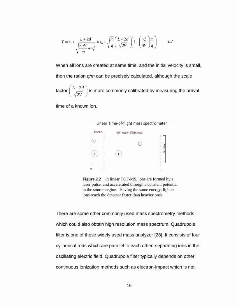
When all ions are created at same time, and the initial velocity is small,

then the ration q/m can be precisely calculated, although the scale

factor 2

2

L d

V

is more commonly calibrated by measuring the arrival

time of a known ion.

There are some other commonly used mass spectrometry methods

which could also obtain high resolution mass spectrum. Quadrupole

filter is one of these widely used mass analyzer [28]. It consists of four

cylindrical rods which are parallel to each other, separating ions in the

oscillating electric field. Quadrupole filter typically depends on other

continuous ionization methods such as electron-impact which is not

Linear Time-of-flight mass spectrometer

+

+

+

+

Source Drift region (flight tube)

de

tect

or

V

Figure 2.2 In linear TOF-MS, ions are formed by a

laser pulse, and accelerated through a constant potential

in the source region. Having the same energy, lighter

ions reach the detector faster than heavier ones.

17

particularly well suited for pulsed work. They have been used in

tandem with a TOF systems, where the TOF system acts as a pre-

filter, allowing the high resolution quadrupole system to separate fine

details. Other high resolution techniques, like ion traps[29, 30], are

similar to quadrupole filters in not producing the wide range of q/m

values necessary for a wide survey for a small sample of analytes,

such as is considered here.

2.2 Room Temperature Ionic Liquids

Similar to conventional solid state salt, room temperature ionic liquids

(RTIL) are comprised of positive and negative ions; however, RTIL is in

a liquid phase at room temperature as described by the name.

Although a liquid, RTIL has the unusual property of a very low vapor

pressure, making it appropriate for use in a vacuum chamber [31]. As

an example, a small sample of RTIL in our experiment situated in our

copper sample holder lasts months with no evidence of evaporation

while the vacuum is maintained at 10-9 torr. This extremely low vapor

pressure stimulated early interest in RTIL research in chemistry as a

new class of non-volatile solvents, although many are toxic. The

extremely low vapor pressure of RTIL in physics guarantees the

stability for use under high vacuum, a property more typical of solids

[32, 33, 34]. An RTIL ionization source has a few primary advantages.

18

First, the liquid surface of RTIL provides a smooth, repeatable

experimental surface. Conventional MALDI surfaces are crystalline

insulators with inhomogeneous initial electric fields that change after

each laser pulse. An inhomogeneous electric field surface distribution

degrades the temporal resolution of the MALDI technique. Secondly,

the liquid RTIL surface refills the evaporated material, so the surface

never changes. Finally, in contrast to conventional MALDI where

ionization builds from collisions of matrix ions and neutrals, RTIL is a

precharged species that can ionize the analyte through potential

ionization or gentle attachment of an RTIL primary cation or anion to

the analyte molecule.

In our experiment, we use one of the most common RTILs: 1-butyl, 3-

methylimidazolium hexafluorophosphate, BMIM+ PF6-. The structure

and mass are shown in Fig. 2.3. BMIM+ PF6- has been well studied and

is commercially available from reliable chemical companies (Sigma-

Aldrich, Fluka #70956, Switzerland). Beyond this, BMIM+ PF6- has the

common properties mentioned above, liquid at room temperature, low

vapor pressure and ionic composition. In our experiments, we have

observed that the negative ion, i.e. PF6- is stable throughout its travel

to the detector, while the BMIM+ ion fragments, producing

Imidazolium+, during its free-flight. This fragmentation is greater with

higher laser power. [BMIM+][PF6-] is transparent to visible light and

19

does not absorb at the wavelength of our Nd:YAG 532nm laser.

However, at high laser intensities, multiphoton absorption does

produce a strong ionization desorption spectrum. Similarly, metal ions,

e.g. chromium ions, also produce an ionization spectrum at similar

laser intensities.

Figure 2.3 Structures of (i) BMIM+, (ii) PF6-, and (iii) Imidazolium+,

the primary fragment of BMIM+. These three ions are the most abundant

species present in our desorption spectra, in addition to any metal ions.

Aside from Imidazolium, there is another remnant BMIM fragment

(56 Da) present in desorption spectra, though it is less stable, and

frequently fragments further.

i)

ii)

iii)

1-Butyl, 3-Methylimidazolium

BMIM+

C8N

2H

15

+

Mass: 139 Da

Imidazolium

C4N

2H

7

+

Mass: 83 Da

Hexafluorophosphate

PF6

-

Mass: 145 Da

20

2.3 Resolution

2.3.1 Definition

In time of flight mass spectrometry resolution is the ability to identify

ions of different ion species in a single spectra. Figure 2.4 displays

copper isotopes from our laser desorption system to illustrate mass

peaks that are well resolved. These mass spectra use a conversion

from the arrival time of the ions to the ions charge to mass ratio, which

is a linear relationship over small mass ranges. So, one can use either

time spectra or mass spectra to illustrate resolution. In this dissertation

we will focus on temporal resolution which relates more closely to

physical process studied.

Figure 2.4 summed 100 shots spectra, displaying

copper isotope peaks

60 61 62 63 64 65 66 67 68 69 700

1

2

3

4

5

m/z

Ion Inte

nsity (

arb

. units)

21

The temporal resolution of a peak in a spectrum defined as the ratio of

its central arrival time t to the spread of arrival times, Δt. We will define

Δt to be the full width at half maximum of the peak (Eq. 2.8).

t

tresolution

2.8

For time of flight mass spectrometry, the mass resolution and the

temporal resolution are simply related. Because the kinetic energy of

the ions are fixed by the acceleration, all the ions will have the same

value of mv2. But, the ion speed and arrival time are inversely related.

vt L 2.9

0vdt tdv 2.10

v t

dv dt 2.11

so the time resolution is the same as the velocity resolution. Using

this, with the constant kinetic energy, we find:

𝑞𝑉 =1

2𝑚𝑣2 𝑣2𝑑𝑚 + 2𝑚𝑣𝑑𝑣 = 0 2.12

𝑣

𝑑𝑣= −

2𝑚

𝑑𝑚 2.13

22

The relation between temporal and mass resolution is thus:

t

t

m

m

2 2.14

Figures 2.5a) & b) display PF6 negative ion peak temporal and mass

resolution which are consistent with Eq. 2.14.

a)

b)

Figure 2.5 Data showing the arrival time of a negative PF6 ion after traveling

0.5 m with an energy of 3KeV in the top graph, and the m/z values in the bottom

graph. The temporal resolution is around 310. Whereas the mass resolution, at

150, is half as large.

23

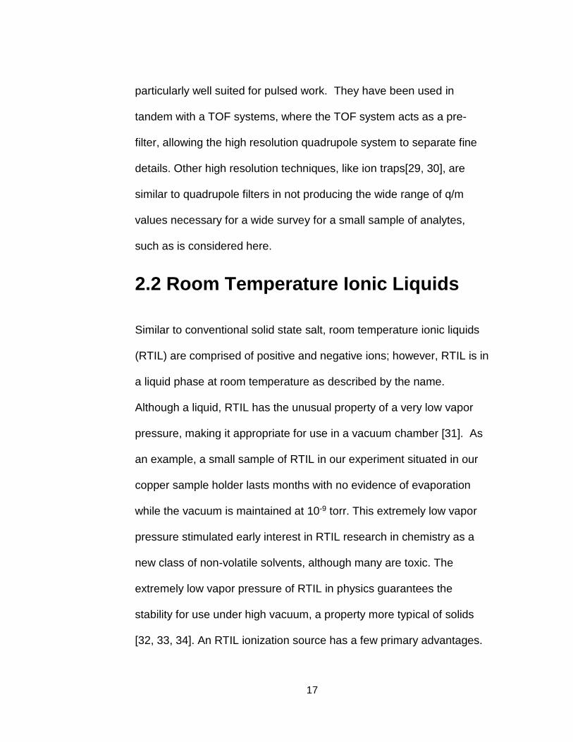
2.3.2 MALDI resolution

Conventional MALDI has fundamental limits on its intrinsic resolution.

The nature of a hot, exploding collisional plume after the desorption

process broadens the initial energies to degrade the resolution. A low

mass spectra produced by conventional MALDI (20kV energy) in figure

2.6 shows this degradation. Within the same mass range, our laser

desorption spectra, Fig. 2.7, of an RTIL ionization source offers better

resolution and peak shape. This improvement in resolution is not an

artificial effect of the acceleration voltage setting, as conventional

MALDI uses much higher voltage than our RTIL desorption.

Figure 2.6 A conventional MALDI, quality control spectra,

taken at EVMS using a Ciphergen PBS2 instrument, displaying

one of the better resolved peaks within the low mass range. This

peak suffers from poor resolution and a distorted peak shape.

205 206 207 208 209 210 211 212 213 214 2150

1

2

3

4

5x 10

4

m/z (Da)

Ion Inte

nsity (

arb

. units)

24

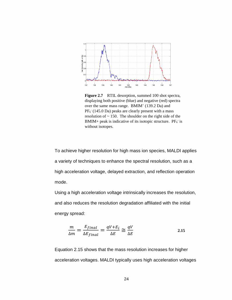
To achieve higher resolution for high mass ion species, MALDI applies

a variety of techniques to enhance the spectral resolution, such as a

high acceleration voltage, delayed extraction, and reflection operation

mode.

Using a high acceleration voltage intrinsically increases the resolution,

and also reduces the resolution degradation affiliated with the initial

energy spread:

𝑚

∆𝑚=

𝐸𝑓𝑖𝑛𝑎𝑙

∆𝐸𝑓𝑖𝑛𝑎𝑙=𝑞𝑉+𝐸𝑖

∆𝐸≅𝑞𝑉

∆𝐸 2.15

Equation 2.15 shows that the mass resolution increases for higher

acceleration voltages. MALDI typically uses high acceleration voltages

Figure 2.7 RTIL desorption, summed 100 shot spectra,

displaying both positive (blue) and negative (red) spectra

over the same mass range. BMIM+ (139.2 Da) and

PF6- (145.0 Da) peaks are clearly present with a mass

resolution of ~ 150. The shoulder on the right side of the

BMIM+ peak is indicative of its isotopic structure. PF6- is

without isotopes.

25

of 10 to 20KV, whereas we restricted ours to 1 to 3KV. High

acceleration voltages produce very fast ions which then require a long

free-flight travel region in order to make the arrival time much longer

than the creation time. A 2 m flight region is not uncommon for a TOF-

MS apparatus, and some also use a reflectron to make the ions travel

twice through the free-flight region. We kept our apparatus simple (no

reflectron) and reasonably short (<0.5 m), and this necessitated that

we use a low acceleration voltage.

Laser desorption typically produces a plume with an average ejection

velocity of 800-1000 m/s, and the velocity spread is a significant

fraction of that. Delayed extraction is probably the most common

arrival time reduction technique [35]. If one delays applying the

extraction voltage for a short time, the faster ions will move farther

away from the sample, so that when the extraction voltage is applied,

the fast ions will travel through a smaller voltage drop. Thus, by the

end of the acceleration region, the initially slow ions will have gained

more energy and will then have a more similar velocity to the initially

fast ions. This technique requires careful tuning of the delay time, and

it only works for a band of ions centered around one value of q/m.

Initially fast ions with a mass lower than the target mass will have

moved too far and will end up with less energy than the slow ions of

the same mass. Consequently, delayed time extraction only narrows

26

the arrival time for ions within a mass-focusing range (which is

determined by the delay time). Figure 2.8 illustrates this technique.

The other common resolution technique is to use a reflectron. Not only

does this increase the effective length that the ions travel, but the

electrostatic mirror that reflects the ion will also decrease the initial

energy spread [36]. More energetic ions travel a longer path by

penetrating deeper into the mirror than slow ions. The detector then

Figure 2.8 Delayed Extraction Schematic. a. Same mass ions with different

initial velocities are allowed to separate spatially, before the application of an

extraction field. b. Extraction field applied such that each ion experiences a

different position based acceleration. c. Same mass ions, each with different final

velocities, arrive simultaneously at detector.

a.

b.

c.

Energy gain due to field

= α*qV0

Applied voltage =V0

α = x/L

x

L

27

collects all the ions at the focal point of electrostatic mirror where all

the arrival times of one species match. A final common approach to

enhance the resolution is to use tandem TOF-MS, which consists of

sequential acceleration and free flight apparatuses, taking only a small

time slice from the first spectrometer as input to the second one.

Any of these TOF-MS methods that depend on a short creation burst

suffer a loss of resolution at high production rates. When the signals in

a single burst are large, then isotopically selected ions show

broadening of the arrival times. This dissertation explores the reasons

for this decrease in time resolution.

MALDI produces decent resolution time of flight spectra with the

incorporated techniques mentioned, specifically at high mass range.

Blood serum peptide of mass 7777 Da in figure 2.9 reveals excellent

resolution from MALDI with incorporation of several of these enhancing

techniques. Our laser desorption from room temperature ionic liquid is

Figure 2.9 Conventional MALDI quality control spectra,

in the high mass range, using delayed extraction, high

acceleration voltage. Peptide of mass 7777 Da with a good

mass resolution of ~600.

7.7 7.72 7.74 7.76 7.78 7.8 7.82 7.84 7.86 7.88 7.90

1000

2000

3000

4000

5000

6000

7000

8000

m/z (kDa)

Ion Inte

nsity (

arb

. units)

28

competitive with conventional MALDI without applying any resolution

enhancing techniques discussed.

29

Chapter 3

Apparatus

This chapter describes components of our experimental apparatus. All

the ionization and detection occurs in a vacuum chamber. The

detection system, consisting of microchannel plates and a collection

plate, sits in the top region of the vacuum chamber and provides highly

efficient ion detection. Outside the chamber, a laser system generates

laser pulses that initiate the ion desorption process. A top-down

illumination reflection system focuses the laser beam onto the surface

of the sample holder inside the vacuum chamber. The data acquisition

system stores and analyzes the experimental data. The following

sections describe the details of each component.

30

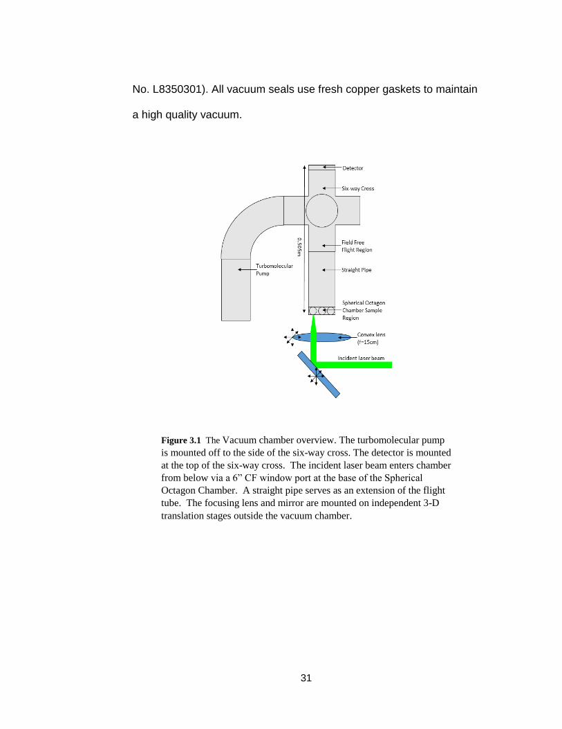
3.1 Vacuum System

The vacuum chamber is constructed from standard stainless steel

components, including a 6 way cross, an 8.5” long full nipple and an

octagonal source chamber, all connected via 6” Conflat flanges. The

octagonal source chamber has eight 2.75” Conflat port windows along

the edge of a ring with a 6” Conflat flange port window below. Figure

3.1 shows the layout of the entire chamber, vertically oriented with the

sample at bottom while allowing laser access from below. The free-

flight region is ~0.5 meter, consisting of a portion of the 6-way cross

and the full nipple flange. The sample assembly sits inside the

octagonal chamber at the bottom adjacent to the windows and the high

voltage feed-through ports.

The entire chamber assembly is mounted in a customized Unistrut

structure, sitting securely on an 8’×4’ optical table. The vacuum pumps

are mounted from an elbow flange on the central 6-way cross. The

pressure in the chamber is maintained at 10-9 torr by a Leybold

Turbovac 152 turbomolecular pump (145 l/s) in combination with a

Varian SD200 Rotary Vane roughing pump (~50 l/s or 180 l/min). The

roughing pump keeps the turbo pump forepressure in the range of 10-4

torr. The pressure is measured by a Varian 0564-K2500-303 Bayard-

Alpert style ionization gauge with a Varian Multigauge controller (Part

31

No. L8350301). All vacuum seals use fresh copper gaskets to maintain

a high quality vacuum.

Figure 3.1 The Vacuum chamber overview. The turbomolecular pump

is mounted off to the side of the six-way cross. The detector is mounted

at the top of the six-way cross. The incident laser beam enters chamber

from below via a 6” CF window port at the base of the Spherical

Octagon Chamber. A straight pipe serves as an extension of the flight

tube. The focusing lens and mirror are mounted on independent 3-D

translation stages outside the vacuum chamber.

32

3.2 Detector and Data acquisition

system

At top of the vertically oriented vacuum chamber is a pair of

microchannel plate (MCP) detectors in Chevron mode coupled to a

stainless steel sheet collector plate (see Figure 3.2). This system

provides excellent gain of ~106 and great temporal resolution. The

0.6 mm thick microchannel plates are made of glass and have 10 um

diameter channels passing through at a 12o angle with respect to the

plate surface. The channels have a 12.5 um separation from center to

center.

Figure 3.2 The microchannel plate detector in Chevron mode uses a

stainless steel collector plate. The plates have a diameter of 25 mm, while

the channels are at a 12° bias angle with a 10 µm diameter and a center to

center channel separation of 12.5 µm.

H.V.

Grounded

H.V.

33

Energetic charged particles striking the interior of a channel wall

generate secondary electrons. This process repeats along the length

of the channel to achieve the large net gain. The bias voltage

accelerates the secondary electrons down the channel though the

plates where the cascade process yields more secondary electrons.

With the front of the first plated grounded and the back of the second

plate biased at +1600V, +1700V or +1800V to record the signal with

reasonable size from collection software, the two plates produce a

combined gain as large as 106. The front of the first microchannel plate

is grounded to maintain zero field in the field free flight region. The

chevron mode of two microchannel plates means these two plates are

positioned with 180 degree rotation to make a “V” configuration. This

setup limits the contribution of false event counts coming from back

streaming positive ions producing another electron cascade after an

energetic channel wall collision.

The secondary electrons are accelerated to the collection plate that is

biased at the same voltage as the second microchannel plate. The

electrical signal is collected after a coupling circuit and recorded by a

DP211 Acqiris Technologies 8-bit digitizer board. A photodiode signal

detects scattered laser light to provide an external trigger for the data

acquisition. This photodiode signal is only used for triggering the

acquisition. The absolute zero time is determined by detecting an

34

single electron signal from a negative ion spectrum. This electron

signal, with 3 KeV energy, arrives at the detector 37 ns after the

electrons have been created. A typically data run consists of 100

single shots, each stored individually. The acquisition program has a

display window and a zoom window to monitor both the entire ion

spectrum of one single shot and a specific ion peak, such as BMIM+,

for live monitoring. The live monitor zoom window is very helpful when

aligning the experimental setup.

3.3 Laser and Optics

The laser that produces the ionization is the second harmonic (532nm)

of a Quanta-Ray DCR-2A ND: YAG laser operating at a 10Hz

repetition rate. This repetition rate is much slower than necessary for

the ~10 μs flight time of the ions we observe. A different laser, running

at rates up to 1 Khz have made data collection much faster in some

systems, but attempts to detect high values of q/m would still

necessitate high numbers of ions, producing the resolution

degradation. A very high repetition rate, such as that of a typical Kerr-

effect short pulse Ti:Sapphire laser (10-20 MHz) would not allow

sufficient time for the ions to travel the free flight region. This could

confuse ions from one pulse with those from other pulses. The spot

35

diameter after the doubling crystal is approximately 1 cm. Figure 3.3a

shows the temporal profiles of one hundred laser shots, as measured

by a photodiode. The pulse widths are nearly constant and the

amplitudes have less than 5 percent (RMS) variation. Figure 3.3b

shows a typical single shot. The Q-switched laser has a central peak

with a full width at half maximum of 5ns, surrounded by two reduced

energy peaks. The relative amplitude of the side peaks is the largest

apparent variation from pulse to pulse. At higher temporal resolution,

Figure 3.3 Temporal profile of ND: YAG laser pulses. In a) 100 laser shots

show a relatively stable pulse with amplitude fluctuations less than 5 percent. In

b) a single shot laser temporal profile shows a central peak width of less than 5ns.

36

we expect the output to show mode beating, as the linewidth is larger

than the Fourier transform limit of the 5 ns pulse duration. The

average power of a single laser pulse was typically 2 mW as measured

by a thermal power meter (Newport model 835) for a net energy per

pulse of 200 μJ.

Since we only needed a small fraction of the laser output we used the

reflection from the front face of a prism placed in the laser path. We

further reduced the laser power using a series of neutral density filters.

The beam enters the vacuum chamber from below, having been

reflected up through the bottom window of the chamber. Inside, it

again reflects from a mirror mounted at 45° with respect to the optical

table. A three dimensional translation stage, mounted outside the

vacuum chamber, positions a 15 cm convex lens to focus laser beam

to a 50 μm spot on the sample surface. The translation stage allowed

us to scan the position of the spot over the entire sample. The focused

laser spot displayed higher order modes with complicated structure

when imaged on black burn paper. Inside the vacuum chamber, the

top-down illumination system reflects the beam to the target surface.

37

3.4 Laser ionization sample assembly

and exchange

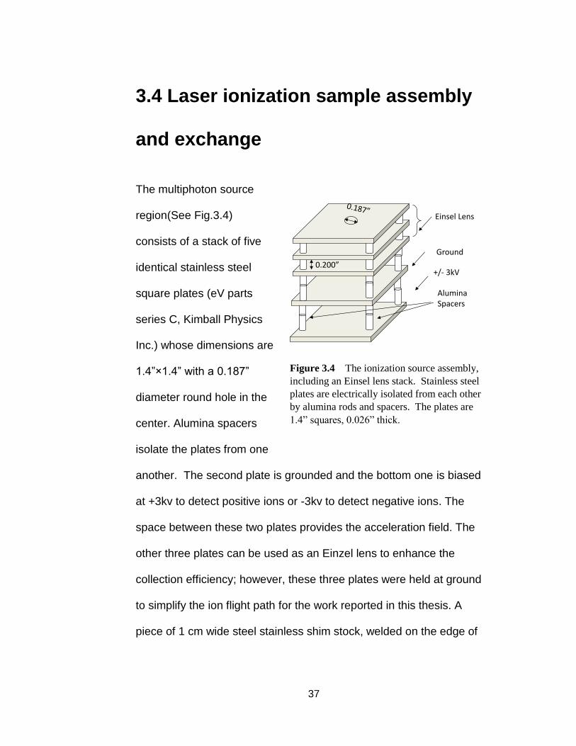
The multiphoton source

region(See Fig.3.4)

consists of a stack of five

identical stainless steel

square plates (eV parts

series C, Kimball Physics

Inc.) whose dimensions are

1.4”×1.4” with a 0.187”

diameter round hole in the

center. Alumina spacers

isolate the plates from one

another. The second plate is grounded and the bottom one is biased

at +3kv to detect positive ions or -3kv to detect negative ions. The

space between these two plates provides the acceleration field. The

other three plates can be used as an Einzel lens to enhance the

collection efficiency; however, these three plates were held at ground

to simplify the ion flight path for the work reported in this thesis. A

piece of 1 cm wide steel stainless shim stock, welded on the edge of

Figure 3.4 The ionization source assembly,

including an Einsel lens stack. Stainless steel

plates are electrically isolated from each other

by alumina rods and spacers. The plates are

1.4” squares, 0.026” thick.

Ground

+/- 3kV

Einsel Lens

Alumina Spacers

0.200”

38

the plate provides the voltage lead. The 2.75” feedthrough flange with

four electrode outputs is mounted on the side window of the octagon

chamber. This multi-plate stack structure hangs above the bottom 6”

CF window, fastened to the side wall by a Groove Grabber system

(Part No: MCF600-GrvGrb-C01, Kimball Physics Inc.) which itself is

mounted to the groove inside the chamber bottom.

The sample holder, a square copper plate with a 5mm diameter well,

0.4 mm deep as in Figure 3.5 sits in the center of the bottom plate,

maintaining good electrical contact. The well in the sample holder is

either filled with RTIL or holds a small metal piece as a test sample.

Figure 3.5 a) Top view of the sample holder. 10mm square with 5mm diameter

well. b) Side view of sample holder. 0.8 mm height with 0.4 mm deep well in

center.

39

The laser beam comes up from below through the bottom of the 6” CF

window and reflects down to the sample in the holder. The top-down

illumination system (Fig.3.6) consists of a mirror mounted inside the

chamber to reflect the laser beam to the sample surface.

The mirror is clamped to a steel stainless ring that is bolted to one end

of a wide stainless steel plate which itself is mounted to another groove

grabber attached to the bottom of the chamber. The mirror is tilted at a

20° angle from the horizontal so that the laser beam hits the target with

an incident angle of 50°. There are two 1 mm wide 0.4 inch long slits

cut into the sides of the 2nd and 3rd accelerator assembly plates to let

the laser beam pass. The beam is focused by a convex 15 cm lens,

outside the vacuum chamber, to form a spot on the target that is

approximately elliptical, approximately 50 μm wide and 80 μm long. We

Figure 3.6 The top down illumination system (a), and a drawing (b) of the

stainless steel plate with a slit.

40

measured the spot size by burning a piece of metal sheet outside of

chamber in the atmosphere and measuring it with an optical

microscope.

In order to change samples, it is necessary to vent the chamber to

atmosphere and open it. Originally, we had used the bottom window

as a point of entry; however, that required realigning the accelerator

stack and the focusing lens after each opening. So, we instead

developed an improved system where we removed one of the side

flanges on the spherical octagon chamber. This method required

removing the sample holder from the side window by carefully using

tweezers, but it had no effect on the top-down illumination system, the

external optics, nor on the electrical connections to the chamber. This

method allowed us to change samples in a few hours, with most of that

time being the time required to pump the system back to a high

vacuum.

41

3.5 System Calibration

When the system gain is set to see small signals, the larger signals

can easily exceed the range limit of the collection software. We

degraded the system gain either by decreasing the detector voltage or

by inserting a 10 dB attenuator to gather high intensity ion signals.

To determine the scale factor so that we could connect the two types

of experiments (with and without the 10 dB attenuator, for example),

we followed this procedure. To calibrate the signal with the 10 db

attenuator, we recorded a series of 100 laser shots while monitoring

the BMIM+ ions. We repeated this process for runs with and without

the 10 dB attenuator at three different laser powers of 0.6 mW, 1 mW,

and 2 mW. Figure 3.7a shows 100 shots of data summed under 1 mW

laser intensity. The large peaks in figure 3.7a were taken without the

attenuator; whereas the smaller peaks used the 10 dB attenuator. The

ratio between the average peak amplitudes of runs under changed

conditions represents the gain scale factor. Figure 3.7b plots integral

signal size under different laser intensities. The error bar is the

standard deviation of multiple measurements under same conditions.

The 10 dB attenuator reduces the signal size by factor of 9.87, (±3%)

which is the slope of the linear curve.

42

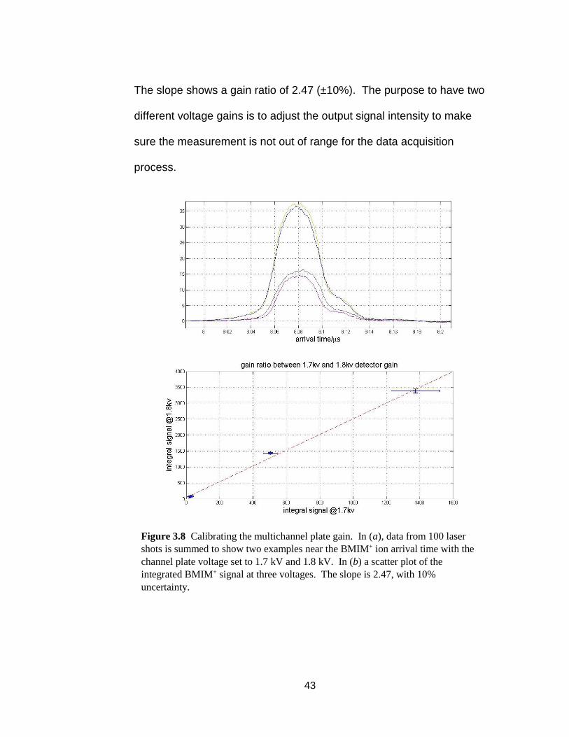
We repeated this process to compare the gain with 1.7 kV and 1.8 kV

bias on the multichannel plates, as shown in Figure 3.8. Figure 3.8a

shows the integrated signal of 100 shots under 1 mW laser intensity.

Figure 3.8b curve shows the comparison of the integrated signals at

the three laser powers at the two different microchannel plate biases.

Figure 3.7 Calibrating the attenuator. In (a), data from 100 laser shots

is summed to show two examples near the BMIM+ ion arrival time with

and without the attenuator near 1 mW laser power. In (b) a scatter plot of

the integrated BMIM+ signal with and without the attenuator at laser

powers of 0.6mW, 1mW and 2mW. The slope is 9.87 with a 3%

uncertainty.

43

The slope shows a gain ratio of 2.47 (±10%). The purpose to have two

different voltage gains is to adjust the output signal intensity to make

sure the measurement is not out of range for the data acquisition

process.

Figure 3.8 Calibrating the multichannel plate gain. In (a), data from 100 laser

shots is summed to show two examples near the BMIM+ ion arrival time with the

channel plate voltage set to 1.7 kV and 1.8 kV. In (b) a scatter plot of the

integrated BMIM+ signal at three voltages. The slope is 2.47, with 10%

uncertainty.

44

Chapter 4

Non-linear Production Process

and Limits on Resolution

This chapter displays the mass spectrum generated in our apparatus

and discusses the resolution decreases with increasing signal size.

Protein and peptide identification in proteomics work strongly relies on

the ability to distinguish ion species and isotopic structures from a vast

cluster of ion species. Conventional MALDI, using high acceleration

voltages and delayed extraction is proficient in determining heavy

mass ions. In the work presented in this thesis, we have used a low

accelerating voltage and no delayed extraction to study why the

resolution decreases with increasing signal sizes.

45

4.1 RTIL data

As introduced in sec. 3.4, the sample holder is either filled with RTIL or

holds a small piece of metal. Figure 4.1 displays a typical average

mass spectra of 100 laser shots on RTIL with +3 kV acceleration

voltage and 2.5 MW/cm2 laser intensity. The dominant peaks are

BMIM+ with an approximate mass resolution of 150 and imidazolium+

which is the main fragment from unimolecular decay of BMIM+. There

are ion peaks at atomic mass numbers 207 and 118 which are Pb+ and

Sn+, the constituents of the solder that binds two copper pieces to

make the sample holder. The minority peaks are atomic mass number

23 and 39, i.e. Na+ and C3H3+, which are contaminants on the sample

surface that occur during the sample preparation.

Figure 4.1 Average mass spectra of 100 laser shots on RTIL with 3 kV

acceleration voltage and 2.5 MW/cm2 laser intensity. BMIM+ and imidazolium+

are ionized from RTIL. Pb+ and Sn+ are components from solder paste on sample

holder while there are minor contaminants at atomic mass number 23 and 39.

46

4.2 Nonlinear ion production process

The ion desorption process exhibits a strong power dependence at

power densities below 10 MW/cm2. Figure 4.2 shows the average

BMIM+ ion signal (over 100 laser shots) as function of laser intensity.

The average BMIM+ production shows a strong nonlinear growth below

10MW/cm2 and rises more slowly above that.

Figure 4.3 plots BMIM+ peaks in the averaged 100 laser shots data

with low and high laser intensity, i.e. 2.5 MW/cm2 and 50 MW/cm2,

from the increasing region and plateau region in Fig. 4.2. The

resolution is worse as average ion production signal goes stronger with

high laser power intensity.

Such a rapid nonlinear increase in the signal size, and such a change

in the line shape, suggests that the shot to shot variation of the spectra

Figure 4.2 BMIM+ average 100 shots integrated signal as function of laser

intensity in logarithmic scale. Ion production experiences rapid rise below

10MW/cm2 and slower growth above. Data are taken under 3kV acceleration

voltage and 50cm free flight distance.

47

might be very large. To illustrate the shot to shot variation, Figs. 4.4

and 4.5 show heatmaps of a single set of 100 laser shots under

relatively low (4.4) or high (4.5) laser intensities near the arrival time of

the BMIM+ ion. The color bar represents the raw ion signal intensity in

volts. Although the higher intensity produces more ions and broader

peaks than the low intensity spectra as shown in Fig. 4.3, the most

remarkable feature is the wild arrival time variation from shot to shot.

Figure 4.3 average BMIM+ peak of 100 data shot run at different laser

intensities. Red is 2.5MW/cm2. Blue is 50MW/cm2.

Figure 4.4 Heatmap displays BMIM+ peaks over the course of 100 data

shots run at 2.5MW/cm2 laser intensity. Color bar represents raw ion

signal intensity in volts.

48

Figure 4.6 shows the variation from shot index number 71 to 74 from

Fig. 4.5. Since all the experimental parameters were fixed, and the

Figure 4.5 Heatmap displays BMIM+ peaks over the course of 100 data shot run

at 50MW/cm2 laser intensity. Color bar represents raw ion signal intensity in

volts.

Figure 4.6 BMIM+ peaks in shots whose index numbers are 71(weaker signal)

and 74 (stronger signal) from high laser intensity data as in figure 4.5

49

laser intensity fluctuations were less than 5%, we believe the large

variation in signal size is due to the strong non-linearity coupled to the

varying hot spots made by the temporal and spatial variation of the

laser. Typically we see about 1 cm-1 linewidth, where the Fourier

transform limited pulus would be 1000 times narrower. So, a limited

pulse has a lot of temporal mode beating that gives “hot” spots lasting

for tens of picoseconds, well below what we can see with our

photodiode. We can see the temporal shot to shot variation in that the

side peaks in the time profile tend to vary much more than the overall

energy. Sometimes the early side peak is smaller that late one,

sometimes reversed. The spatial modes are even worse. The laser

spot is pretty far from a single mode Gaussian beam – even before the

doubling crystal, which empasizes hot spots. We routinely see

structure in our burn patterns such as hot ares that are a millimeter or

out of 1 cm beam. So, this likely give rise to (non-repeatable) hot spots

that are ten time smaller than nominal focused laser spot. All of this

means that the small time and small space variation of the laser pulse

intensity is much greater than 5% overall energy variation we

observed.

50

4.3 Resolution Degradation

4.3.1 Ion production dependence

Figure 4.3 shows that the resolution has degraded in the shots with

higher laser intensity. Figure 4.6 shows that, even with the same

nominal laser intensity, a spectrum with high ion production has

significantly worse resolution than a spectra with lower ion production.

To explore the pattern of resolution related to ion production, Fig. 4.7

represents 700 laser shots with the nominal laser intensity fixed at 50

MW/cm2, showing the data near the positive BMIM+ ion time location,

following 3 kV acceleration and 50 cm of free flight distance. Data are

from different dates and different sample locations by moving laser

spot locations are combined in this figure. The heat map in Fig. 4.7

Figure 4.7 Heatmap displaying a 700 shot data run of positive 3 kV BMIM+

peaks. Shot index are sorted by total ion production. Laser intensity is 50

MW/cm2. Free flight distance is 50 cm.

51

differs from that in Figs. 4.4 and 4.5 by being sorted in order of

increasing total ion signal.

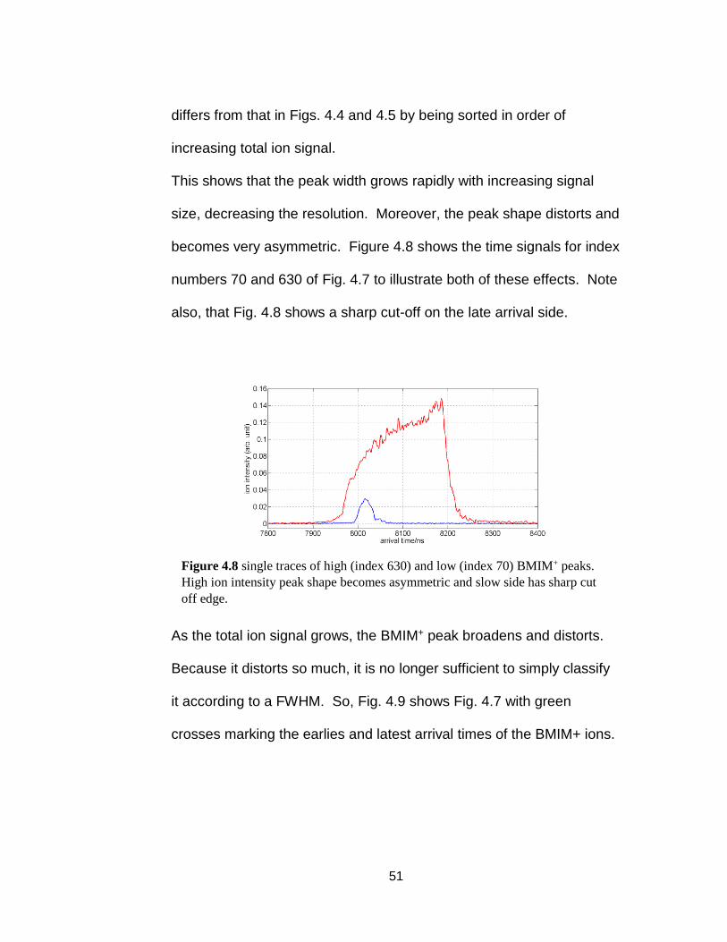
This shows that the peak width grows rapidly with increasing signal

size, decreasing the resolution. Moreover, the peak shape distorts and

becomes very asymmetric. Figure 4.8 shows the time signals for index

numbers 70 and 630 of Fig. 4.7 to illustrate both of these effects. Note

also, that Fig. 4.8 shows a sharp cut-off on the late arrival side.

As the total ion signal grows, the BMIM+ peak broadens and distorts.

Because it distorts so much, it is no longer sufficient to simply classify

it according to a FWHM. So, Fig. 4.9 shows Fig. 4.7 with green

crosses marking the earlies and latest arrival times of the BMIM+ ions.

Figure 4.8 single traces of high (index 630) and low (index 70) BMIM+ peaks.

High ion intensity peak shape becomes asymmetric and slow side has sharp cut

off edge.

52

Figure 4.10 illustrates the process to find out these arrival times with

single shots in Fig. 4.6. Within a time window larger than the broadest

BMIM+ peak, we have determined the times when the signal is 10% of

its maximum value during the peak. We will define a full time width of

Figure 4.9 Heatmap as figure 4.7. Green cross dots are earliest and slowest ion

picked out.

Figure 4.10 process to find out earliest and latest BMIM+ ion in each single shot

53

each peak as the difference between the earliest and the latest of

these points. Figure 4.11 represents the growth of the BMIM+ full width

versus total summed ion signal intensity.

4.3.2 Ejection time spread in resolution

The two major contributions to a changing width are changes in the

initial velocity distribution and changes in the initial ion ejection time.

Chapter 2 showed the relationship between energy ( or velocity)

spread and arrival time spread to be

𝑑𝑣

𝑣= −

𝑑𝑡

𝑡=𝑑𝐸

2𝐸 4.1

Figure 4.11 BMIM+ peaks full width in terms of total ion intensity.

In high intensity region, it is a linear curve. Data are positive 3 kV and 50 cm free

flight distance.

54

Under same acceleration voltages, if the resolution degradation is

mainly due to initial velocity spread, the time spread should be linearly

dependent on the travel time or the free field flight distance. In our

experiment, we placed the detector at three different locations,

specifically 50 cm (called “far”), 25 cm (called “intermediate”) and 10

cm (called “near”) from the ion desorption source. Figure 4.12 shows

the full widths of the BMIM+ peaks collected with the three detector

positions. The blue dots are results from the 5 0cm free flight (far

detector). The red dots are results from the 25 cm free flight

(intermediate detector), and the green circles are results from the 10

cm free flight (near detector). The peak widths follow the same shape

of functional dependence for the near and intermediate detector

positions. This suggest strongly that the width increase is not due to a

velocity spread. If the width were due to a velocity spread, the red

Figure 4.12 BMIM+ peak width versus total ion signal from 50 cm (blue), 25

cm(red) and 10 cm(green) detector position. Data are taken with 3 kV

acceleration voltage and 1.7 kV detector gain.

55

circles would have risen at a rate 2.5 times faster than the green

circles. The far detector data seems inconsistent with this at first sight;

however, most of that data shows a lower total signal size. Our

simulation in the next chapter will show that this apparent increase is

due to the expansion of the ions to fill a spot much larger than the

detector, effectively reducing the detector efficiency by a factor of 2

approximately. If the data were corrected for this loss of ions, all three

detector position would produce the same curve, demonstrating that

velocity spread is not the major cause of the linewidth change.

Before check width dependence on energy, we need to know the

detection efficiency of the microchannel plate detector is dependent on

the incident impact energy of an incident ion. In this experiment, 2kV

and 3 kV are our standard acceleration voltages leading to different

detection gains. To calibrate the efficiency with different energies, we

collected BMIM+ data with 2 kV and 3 kV sequentially under the same

detection voltage and laser intensity conditions. Sorting the signal size

with different total energies, the correlation between collected ion

productions explicitly illustrates the efficiency difference BMIM+ ions

with either 3 kV or 2 kV total energy (Fig 4.13). Assuming that the total

distribution of the production of BMIM+ ions was the same for the

56

sequential runs, we find that the higher energy ions produce a signal at

the detector that is 1.95 (±3%) times larger than the lower energy ions.

As an additional check on the origin of the linewidth growth, we

measured the dependence of the linewidth on the acceleration energy.

Figure 4.14 shows the growth of the peak width of the BMIM+ when

accelerated by either 2 kV or 3 KV. If the linewidth were due to a

velocity (or energy) spread, then the increasing the acceleration

energy would reduce the linewidth for two reasons: (1) the initial

energy spread would be a smaller fraction of the total energy, and (2)

the arrival time would decrease. The 2 kV summed ion signal intensity

has been increased by the 1.95 factor in accordance with the reduced

detection efficiency shown in calibration.

Figure 4.13 Correlation of BMIM+ data taken with 3kV and 2kV acceleration

voltage. The detection gain ratio is 1.95 to calibrate ion data with different

energy.

57

Figure 4.15 represents the peak width growth with ion signal increase

for different initial electric field amplitudes. All of these BMIM+ data

Figure 4.14 Scattered dots display of the BMIM+ peak width in term of total ion

production. Green dots represents 3 kV total energy data while red dots represents

2 kV energy data. Both data are taken in the near detector setup, i.e. 10 cm free

flight distance.

Figure 4.15 Scattered dots display BMIM+ peak width in term of total ion

production. Green dots represents 3 kV energy in 0.4 inch long electric field.

Red dots represents 1 kV in first 0.4 inch electric field and 2 kV in next 0.4 inch

electric field with 3 kV total energy.

58

were taken with the detector in the near position (10 cm free flight).

The green dots are data taken in the normal condition of 3 kV

accelerating voltage across with a 0.4 inch plate separation. To change

the field without changing the total energy, we applied 1 kV across the

first set of plates (0.4 inch separation), followed by 2 kV across the

second set of plates. For these data, the red dots in Fig. 4.15, the

extraction field is smaller by a factor of 3. This shows that under same

ion production conditions, the peak width grows faster in a weaker

extraction field.

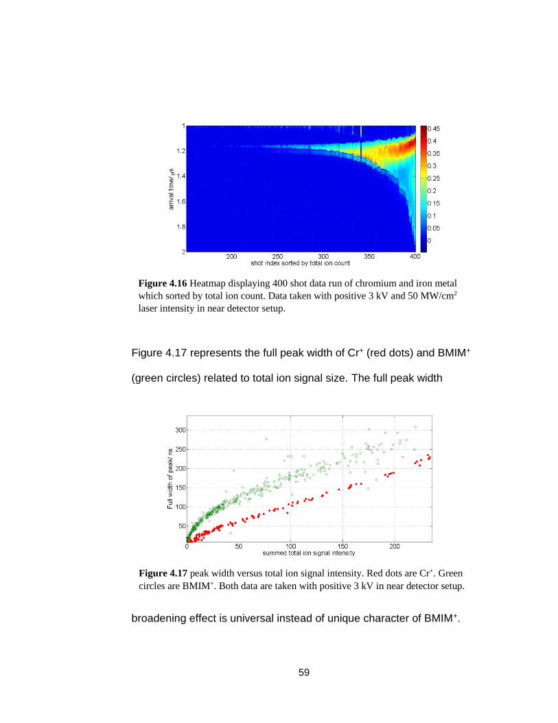
To verify if the peak broadening is universal, rather than being a

characteristic of the RTIL (which does undergo a unimolecular

decomposition during the free flight), we used a polished piece of

metal containing both chromium and iron. Figure 4.16 displays 400

laser shots sorted by the total ion count (with 3 kV acceleration volts

and a 50mW/cm2 laser intensity). Figure 4.16 shows a similar peak

width increase with ion signal growth.

59

Figure 4.17 represents the full peak width of Cr+ (red dots) and BMIM+

(green circles) related to total ion signal size. The full peak width

broadening effect is universal instead of unique character of BMIM+.

Figure 4.17 peak width versus total ion signal intensity. Red dots are Cr+. Green

circles are BMIM+. Both data are taken with positive 3 kV in near detector setup.

Figure 4.16 Heatmap displaying 400 shot data run of chromium and iron metal

which sorted by total ion count. Data taken with positive 3 kV and 50 MW/cm2

laser intensity in near detector setup.

60

This chapter has shown that the mass arrival times broaden with

increasing total ion production causing a degraded resolution when all

other experimental conditions (acceleration voltage and field, travel

distance, and laser power) are held constant. For ions with same

charge to mass ratio, the resolution as measured by arrival time

depends on initial electric field strength rather than on the total energy

gained from the acceleration field. Thus, the resolution degradation is

not due to an increase in the initial ion thermal distribution. Instead the

initial ejection time spread has the greatest contribution to the peak

width broadening. One hypothesis is that space charge from the

ejected ions will weaken the electric field near the ion source to

prevent other ions leaving until the already ejected ions are

accelerated out of the source region. This leads to an initial ejection

time spread that degrades the resolution. We will elaborate models

that simulate this space charge effect fully in the next chapter.

61

Chapter 5

Simulation

As shown in the last chapter, ions continue to escape into the

acceleration region for a longer time as total ion production grows. In

this chapter, we first present a simple model to simulation space

charge effect. Then mean field model simulates space charge effect

and image charge effect at large scale of ion quantities. Ion reservoir

modification describing initial ion distribution successfully fits

experiment data, combing with mean field model. Lastly, slices model

with GPU computing technique dispels concern of accuracy for high

multiplier in mean field model.

62

5.1 Particle Solutions of the Space

Charge Model

To study the behavior of a large quantity of collisionless ions, we

started by simulating each individual ion’s trajectory, solving the motion

and the electric fields of all the ions simultaneously. Equation 5.1

shows the force on each individual collisionless ion, where the first

term is the force from the other ions and the second term is the force

from the external applied electric field. Equation 5.2 shows the

differential ion movement under the net force.

𝐹𝑖⃗⃗ =1

4𝜋𝜀∑

𝑒𝑖𝑒𝑗

𝑑𝑖𝑗2→

𝑛𝑖≠𝑗 + 𝑒𝑖𝐸0⃗⃗⃗⃗ = 𝑚𝑎𝑖⃗⃗ ⃗ 5.1

𝑣𝑖⃗⃗⃗ = 𝑣𝑖−1⃗⃗ ⃗⃗ ⃗⃗ ⃗⃗ + 𝑎𝑖⃗⃗ ⃗𝑡 𝑑𝑙 =1

2∗ (𝑣𝑖−1⃗⃗ ⃗⃗ ⃗⃗ ⃗⃗ + 𝑣𝑖⃗⃗⃗ )𝑑𝑡 5.2

A solution requires initial conditions for each ion. Setting those initial

conditions defines a model.

For our first model we wanted to explore the effects of the ion space

charge during the ions nominally free-flight to the detector. So, we

assumed that the external electric field swept away all of the electrons

immediately. When we used a negative 3kV bias to accelerate

negative ions in the experiment, we found that the electrons arrived at

63

the detector in 7ns, so reversing the field will remove the electrons in a

time much shorter than the ion travel time, justifying our assumption

that they have been swept away. For our ion initial conditions, we

used a uniform distribution over a thin disk. We chose the thickness to

match the distance a free ion would travel in the applied electric field

during a laser pulse time, i.e. 5ns. We chose the radius of the disk to

match the semi-minor axis of the laser spot. This model simplifies the

complex lase desorption process by only considering ions without

electrons after laser pulse.

5.1.1 Matlab ode45 solver

We first used the Matlab ode45 function to solve these differential

equations. Figure 5.1 shows the arrival time distribution of 100 ions

Figure 5.1 arrival time distribution of 100 ions from space charge model with

Matlab ode45 solver.

64

whose mass is 52 atomic mass units (Cr+) at a detector that is 50 cm

from the acceleration region. When the number of ions is small (~100),

the arrival time matches the 4749ns expectation time and the peak is

symmetric.

Figure 5.2 shows similar results for 1000 ions and 8000 ions. The

arrival time distribution becomes broader and starts to show

asymmetry as the ion production increases. But as opposed to our

experiment data, in the simulation more ions shift to earlier times than

to slower times.

There are a couple of crucial disadvantages with this method and

model. First, the calculation is time consuming. For the 1000 ion case,

Figure 5.2 Simulated time distributions for several values of ion counts. Blue:

100 ions. Green: 1000 ions. Red: 8000 ions. Peak width is broader but there are

more earlier ions instead of more slower ions shown in our experiment data.

65

the code ran for approximately 4 hours with Intel® Core™ i7-3770

CPU and 12 gigabytes memory. For the 8000 ion case, it ran over 100

hours. Second, due to high dimensional matrix manipulation (~N2), this

method would require 12 gigabytes of memory for 10,000 hours, and

would stop with an out of memory message for a calculation using over

16000 ions. This method seems unlikely to be extendable to the

100,000-1,000,000 ion cases we believe are necessary to model our

experiment. In addition, the simple ion distribution in this model is

unlikely to represent the real situation when a large space charge

begins to affect the ions during their first stages of acceleration.

In the next coming sections, other simulation models and techniques

will eliminate these issues and explain our observed ion behavior.

66

5.1.2 Customized Fixed Time Step Solver

Initially, the ions move very slowly, and we did not expect that the

solution should require sophisticated integration techniques. So, we

wrote our own matlab code to solve for the ions motion using a fixed

calculation time step of 0.5 ns. The general process is similar to using

the ode45 function to solve the differential equations of Eqs. 5.1 & 5.2.

However, by avoiding the adaptive time steps of the Matlab ode45

function, we have significantly reduced the calculation time. Figure 5.3

shows that the Matlab solution and our code produce very similar

Figure 5.3 8000 ions simulation compare ode45 runtime with own fixed time

step solver. The final distributions are almost the same and calculation time is

much shorter with fixed time step solver.

67

results for the 8000 ion arrival time distribution. The calculation time

with this fixed time step code is approximately 24 hours, which is less

than one fourth of calculation time using the ode45 solver.

5.2 Mean Field Model

As stated above, the ion-ion iterative binary interaction approach to

delaying space charge has severe limits on the total number of ions we

can start in a simulation. Moreover, the ion arrival time distribution

shows calculated this way does not show the enhanced delay as we

observed in experiment. In this section, we will introduce several

improvements to the basic model: we will include the effect of an

image charge created by the first acceleration plate being held at a

constant potential, and we will extend the calculation to larger total

charge by introducing a multiplier, so that each point represents a large

number of ions within a small volume.

68

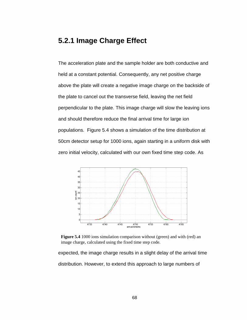
5.2.1 Image Charge Effect

The acceleration plate and the sample holder are both conductive and

held at a constant potential. Consequently, any net positive charge

above the plate will create a negative image charge on the backside of

the plate to cancel out the transverse field, leaving the net field

perpendicular to the plate. This image charge will slow the leaving ions

and should therefore reduce the final arrival time for large ion

populations. Figure 5.4 shows a simulation of the time distribution at

50cm detector setup for 1000 ions, again starting in a uniform disk with

zero initial velocity, calculated with our own fixed time step code. As

expected, the image charge results in a slight delay of the arrival time

distribution. However, to extend this approach to large numbers of

Figure 5.4 1000 ions simulation comparison without (green) and with (red) an

image charge, calculated using the fixed time step code.

69

ions, we had to use a cell approach, where each cell represented a

large number of ions.

5.2.2 Mean Field Model with Multiplier

The limits on our by computer hardware made it impossible to simulate

tens of thousands of ion trajectories. In our mean field model, each

single ion cell represents a large number (called a multiplier) of ions in

the same cell. The trajectory of a cell is calculated just if a single ion

were at its center location, but this trajectory is then applied to all the

ions in that cell. The electric force on each ion in the cell is calculated

from the fields due to all other cells, the image charges and the applied

electric field. This model is similar to the widely used particle in cell

(PIC) model of ion simulation [37, 38, 39]. Our model differs from PIC

models by not allowing ion exchange among cells and by our

assumption that ions in the same cell produce no average force on the

cell center location. By varying the multiplier (the net number of ions in

a cell), we could easily extend our code to an arbitrarily large total

number of ions.

In figure 5.5, we compare a simulation of 40,000 versus 2,000,000

BMIM+ ions, using 2000 cells with multipliers of 20 and 100,

respectively. Ions are initially uniformly distributed in a 1 μm high disk

70

with a 25 μm radius. This simulation uses a near detector (at 10 cm),

and shows a large shift towards longer times, similar to our

experiment.

For a sufficiently large number of ions, the combined fields of the ions

already moving out into the acceleration region, and the image charge

of those ions behind the acceleration plate surface, can entirely cancel

out the applied acceleration field, and even reverse its direction. In this

case, some ions can be accelerated back towards the acceleration

plate. Thus the net number of ions leaving the acceleration plate can

oscillate, as shown in Fig. 5.6. For this figure, we used a total of 0.2

million ions distributed uniformly in a 1 μm high disk with a 25 μm

radius. We do not expect this oscillatory behavior to be observed at

this level because it depends on the removal of all the electrons so that

Figure 5.5 Time distributions of 40 thousands (green) and 0.2 million (red) ions

generated using the mean field simulation code.

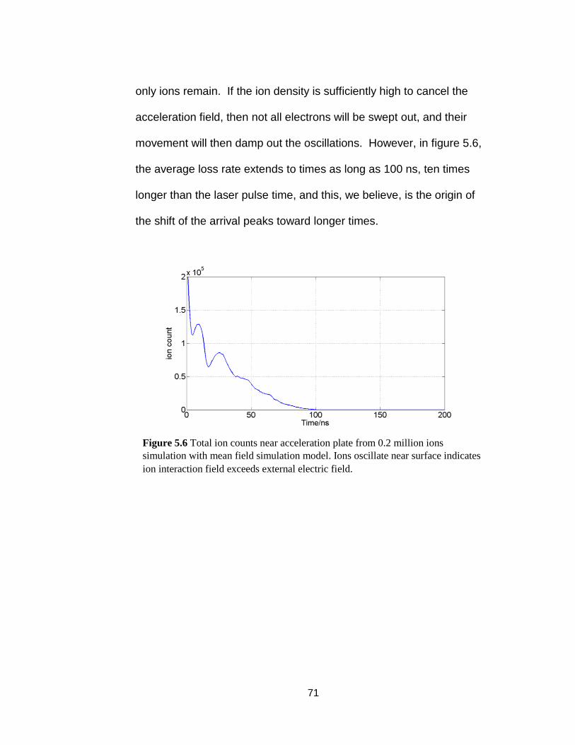
71

only ions remain. If the ion density is sufficiently high to cancel the

acceleration field, then not all electrons will be swept out, and their

movement will then damp out the oscillations. However, in figure 5.6,

the average loss rate extends to times as long as 100 ns, ten times

longer than the laser pulse time, and this, we believe, is the origin of

the shift of the arrival peaks toward longer times.

Figure 5.6 Total ion counts near acceleration plate from 0.2 million ions

simulation with mean field simulation model. Ions oscillate near surface indicates

ion interaction field exceeds external electric field.

72

5.2.3 Ion Reservoir Model

It is beyond the scope of this work to include the electron behavior

under conditions where the space charge and the image charge both

cancel the acceleration field. Instead, we have used an ion reservoir

model, for which we have manually constructed a thin region on top of

the acceleration plate filled with an electrically neutral combination of

ions plus electrons, in which the net electric field is zero. Ions initially

escape from the reservoir at the common laser desorption initial

velocity of 1 km/s. However, once the longitudinal net electric field at

the location of the ion in the reservoir is reduced below a launching

threshold field, which is a small fraction of the unshielded acceleration

field, the ion ejection ceases. As the ejected ions continue to move

away, the field will again decrease, allowing more ions to escape (with

their equivalent electrons flowing into the acceleration plate). The net

effect is that the ion production rate matches the rate that ions leave

the acceleration region. This model reduces the ion oscillations and

produce a slowly decaying ion source after the laser pulse. Figure 5.7

shows the results of this model compared to experimental work with

the detector at 10 cm from the source. The green circles are time

distributions of BMIM+ sample with 10 cm detector setup at 3 kV

acceleration volts. The red curve with dots are simulation results using

73

a reservoir thickness of 3µm, an initial ion distribution radius is 25µm,

and an initial transverse velocity from 0 to 300m/s uniformly and an

initial longitudinal velocity of 1km/s.

To calibrate the measured total ion signal to the simulation total ion

count, we matched a broadened, symmetric, experimental peak shape

to a 40 thousand ion simulation, as shown in Fig. 5.8. We compute a

conversion factor as the ratio between integral of the chosen shot

signal and 40 thousand. Figure 5.9 compares 4×105 ion count

simulation peak with real data whose count is the same estimated from

total signal multiplied by conversion factor. Current model predicts

BMIM+ behavior under strong external electric field fairly well.

Figure 5.7 Simulation of BMIM+ in a 3 kV/cm external electric field. Green

circles are experiment data. Red curve with dots is outcome of simulation.

Reservoir thickness is 3µm, initial ion distribution radius is 25 µm, birth

transverse velocity is from 0 to 300m/s and birth longitudinal velocity is 1 km/s.

74

Figure 5.9 with conversion factor calculated by low ion count, high ion counts

(0.4 million, green) simulation outcome has comparable peak width to high

integral signal shot from experiment data (red).

Figure 5.8 low ion count data (red) shot (total integral signal is 6) versus

simulation outcome (green) with similar peak width (40 thousands ions).

Conversion factor between ion counts and integral signal is determined as

20000/3.

75

Figure 5.10 shows a comparison of experimental data to a simulation

of Chromium ions (mass is 52) with same model and parameters as for

the BMIM+ (mass = 139) case. The experimental data closely matches

the simulation, although there appears to be a systematic difference at

low ions counts. We believe that the presence of other ion species,

especially iron whose mass is close to chromium affects the peak

shape of chromium. At higher ion counts, these effects are minimized.

Figure 5.10 simulation outcome compared with Cr+ ions from experiment data.

External field is 3kV/cm. Reservoir thickness is 3µm, initial ion distribution

radius is 25µm, birth transverse velocity is from 0 to 300m/s and birth

longitudinal velocity is 1km/s.

76

5.2.4 Simulation Parameters Discussion

There are three main parameters to describe our reservoir model: the

reservoir radius, the launching field required to eject an ion from the

reservoir, and the reservoir thickness. We chose the radius of the

reservoir to be the same as the laser spot size; however, the laser spot

is elliptical, rather than circular. Consequently, we have tested the

reservoir model to see if it is sensitive to the initial shape. Our

simulations show that the ions are more quickly ejected from the edges

of the reservoir, where there is less shielding of the acceleration field,

so an ellipse quickly devolves into a more circular shape. Figure 5.11

compares the arrival times of ions from elliptical and from circular initial

Figure 5.11 circular initial ion distribution (green) versus elliptical initial

distribution (red). Final time distribution is independent of initial ion distribution

shape under same charge density. Reservoir thickness is 3 µm, initial ion

distribution is elliptical whose semi-major axis is 35 µm and semi-minor axis is

18 µm. Birth transverse velocity is from 0 to 300 m/s and birth longitudinal

velocity is 1 km/s.

77

ion distributions with 2000 ion cells multiplied by 200 (for a total of

400,000 equivalent ions). The semi-major axis of the ellipse is 1.4

times larger than the radius of the circle while the semi-minor axis is

1.4 times smaller (keeping the area constant). For the same initial

charge density, both spot shapes provide almost the same arrival time

distribution. In the simulation, ions move out of the reservoir only when

the average field in a region near the surface of the reservoir is above

a threshold, which we call the launching field. As shown earlier, this

serves to eliminate ion oscillations in the reservoir without requiring a

full scale calculation of the electron motion. Figure 5.12 compares

simulations of the arrival time distribution for 4 million BMIM+ ions at 3

kV/cm electric field using two different threshold ejection fields of 1%

Figure 5.12 Launching field threshold comparison. Green distribution threshold

is set at 5% of external electric field. Blue is set at 1% of external electric field.

Both are 4 million BMIM+ case in 3kV/cm external electric field. Reservoir

thickness is 3µm, initial ion distribution radius is 25µm, birth transverse velocity

is from 0 to 300m/s and birth longitudinal velocity is 1km/s.

78

and 5% of the applied acceleration field. This change in the threshold

field has almost no impact on the final time distributions.

Due to the complicated laser pulse shape, and the highly non-linear

ionization process, the effective laser pulse length is another

uncertainty in our experiment. Figure 5.13 compares time distributions

with different effective length of laser pluses, i.e. 5 ns and 10 ns.

Excluding laser pulse length variance, the difference is less than 10%

which has no significant influence on simulation outcomes so that there

is no need to be concerned with effective laser pulse length variance in

our simulation.

Figure 5.13 simulation outcomes with 5 ns (green) and 10 ns (red) wide laser

pulse. Peak width variance is less than 10 percent. Reservoir thickness is 3 µm,

initial ion distribution radius is 25 µm, birth transverse velocity is from 0 to 300

m/s and birth longitudinal velocity is 1 km/s.

79

The reservoir thickness is the most sensitive parameter for the

simulation. In Figure 5.14, we compare simulations with different

reservoir thicknesses for BMIM+ accelerated through fields of

approximately 3 kV/cm. Peaks with the same total ion count become

narrower when the simulation uses a larger reservoir thickness.

The electrons always respond to an electric field quickly. After

desorption with some initial energy, the electrons will move upwards

until their velocity slows to zero and becomes negative. The returning

electrons will build a sheath to shield the external electric field from

penetrating into the neutral quasi-plasma near the target surface. We

chose the maximum height the initial electrons could reach as our

reservoir thickness choice. The cold electrons with 1 eV initial energy

Figure 5.14 BMIM+ in strong field simulation with different reservoir thickness.

Blue is outcome of 5 µm thick reservoir. Red is 3 µm and purple is 1 µm. Higher

reservoir will narrow the peak width under the same quantity of ions.

80

will reach to about 3 µm in 3 kV/cm field, while electrons with the same

1eV energy will continue to 9 µm in a smaller 1 kV/cm. Figure 5.15

shows simulation results when an applied 1 kV/cm electric field is used

in first 1 cm and 2 kV/cm field in next coming 1 cm which guarantee

same 3 kV energy as in regular 3 kV/cm experiment setup with 9 µm

thick reservoir. The simulation fits experiment data well from low to

high ion production range for the weak field test.

Figure 5.15 BMIM+ simulation in weak field, i.e. 1kV/cm throughout the first

centimeter and 2 kV/cm in the second centimeter to maintain 3 keV as the total

energy. The red curve was constructed using a 9µm reservoir thickness. The

initial ion distribution radius is 25 µm, initial transverse velocity has a random

distribution from 0 to 300 m/s. The initial longitudinal velocity is 1 km/s.

81

5.2.5 Collection Efficiency Decrease after

long flight

From our simulation of BMIM+ ions in a 3 kV/cm external electric field,

we find that the electrostatic repulsion spreads the ion beam so that

some of ions miss the detector when it is 50 cm from the source.

Figure 5.16 displays time distribution of 4×105 BMIM+ ions reaching the

detector at 50 cm, after being accelerated through 3 kV. The red curve

is the arrival time distribution of all the ions, whereas the blue curve

shows the arrival times of only those ions within a 1.25 cm radius of

the center of the detector. The active region of the detector is a

1.25 cm radius circle.

Figure 5.16 0.4 million BMIM+ time distribution at 50 cm detector with 3

kV/cm electric field. Red is distribution collecting all ions. Blue only collects

ions within detector dimension at 50 cm.

82

Figure 5.16 shows the collection efficiency to be 44% in this case.

Figure 5.17 compares the reduced collection simulation to the data

from a single laser shot, whose total ion production we estimate to be

close to 4×105.

In Fig. 5.17, the peaks widths are equivalent and both show a sharp

cut-off edge on the late arrival side. Similar simulation runs with

different ion productions from 40 thousand to 1.2 million show similar

reductions in the collection efficiency. Figure 5.18 shows good

agreement between our collected data and our simulations for both the

near and far detector positions, as long as the decreased collection

effects are included for the far detector.

Figure 5.17 Time distribution of simulated 0.4 million BMIM+ ions collected

(Blue) by detector compares to a similar ion production shot in experiment data

with the detector at 50 cm from the ion source (Green).

83

5.4 Azimuthally symmetric slices model

The Vlasov equation describes the time development of the distribution

function of a collisionless plasma composed of charged particles

interacting via the Coulomb force. In our model, the Vlasov equation

would properly account for the cell movement, but also for the

movement of ions between cells due to a velocity gradient. To test this

we developed a slice model that reduced the volume, and replicated

that volume with azimuthally symmetric slices that filled the space. In

this case, we could reduce the number of ions in a cell, but make the

Figure 5.18 Time spread of BMIM+ ion at 3kV/cm source electric field. Green

dots are experiment data of detector at 10cm. Pink are data of detector at 50cm.

Red and blue curves are simulation outcome collecting ions within detector radius

1.25cm at 10cm and 50cm far from ion source.

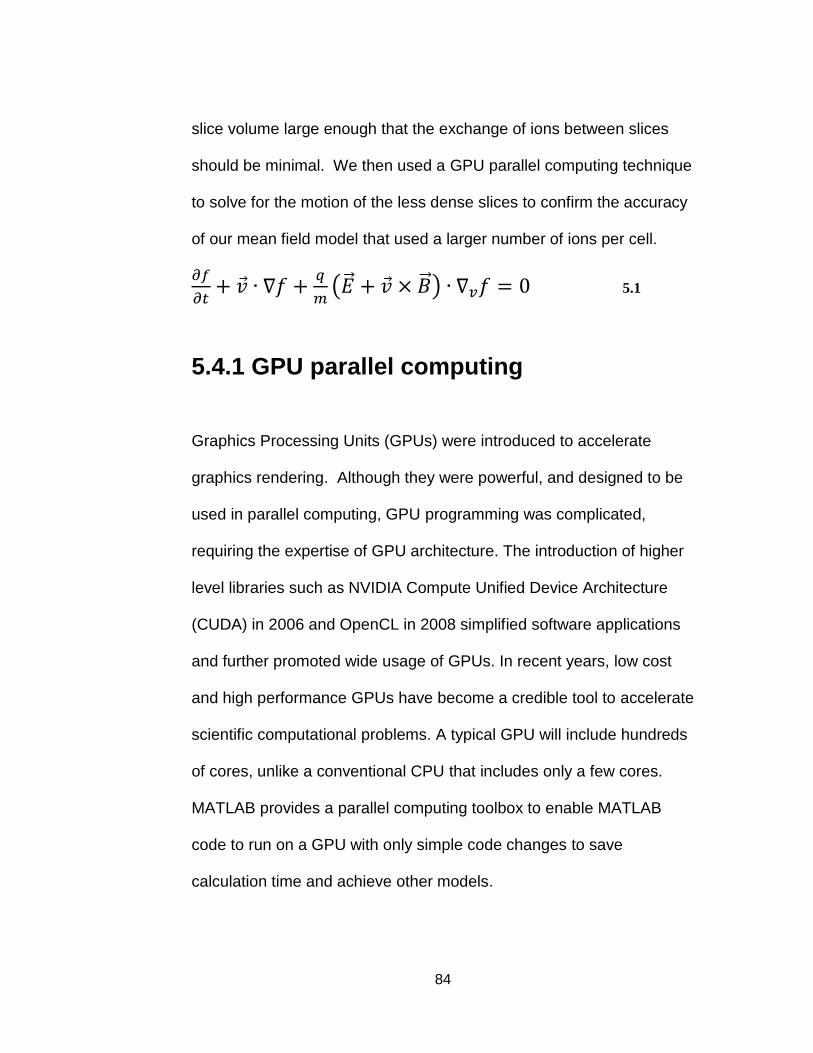
84

slice volume large enough that the exchange of ions between slices

should be minimal. We then used a GPU parallel computing technique

to solve for the motion of the less dense slices to confirm the accuracy

of our mean field model that used a larger number of ions per cell.

𝜕𝑓

𝜕𝑡+ 𝑣 ∙ ∇𝑓 +

𝑞

𝑚(�⃗� + 𝑣 × �⃗� ) ∙ ∇𝑣𝑓 = 0 5.1

5.4.1 GPU parallel computing

Graphics Processing Units (GPUs) were introduced to accelerate

graphics rendering. Although they were powerful, and designed to be

used in parallel computing, GPU programming was complicated,

requiring the expertise of GPU architecture. The introduction of higher

level libraries such as NVIDIA Compute Unified Device Architecture

(CUDA) in 2006 and OpenCL in 2008 simplified software applications

and further promoted wide usage of GPUs. In recent years, low cost

and high performance GPUs have become a credible tool to accelerate

scientific computational problems. A typical GPU will include hundreds

of cores, unlike a conventional CPU that includes only a few cores.

MATLAB provides a parallel computing toolbox to enable MATLAB

code to run on a GPU with only simple code changes to save

calculation time and achieve other models.

85

5.4.2 Slices Model

The slices model and the mean field model only differ in the volume

occupied by the cells and by the number of ions in each cell. The slices

model uniformly distributes hundreds of ions in a small circular sector

whose central angle will be less than 10 degree and then replicates

that sector to build a full circular distribution. Using the overall

azimuthal symmetry, the slice model simulation ignores ion movement

in the azimuthal direction and only tracks ion movement in the radial

and height directions for a single sector. Each ion in the sector feels

the force of the other ions in the sector, and the force from the

replicated versions of all the ions (including itself) in the other sectors.

Figure 5.19 CPU and GPU architecture comparison

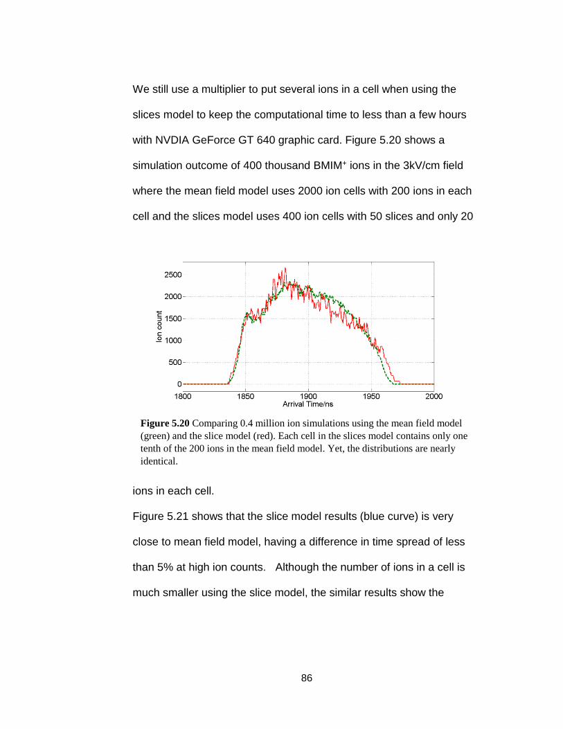
86

We still use a multiplier to put several ions in a cell when using the

slices model to keep the computational time to less than a few hours

with NVDIA GeForce GT 640 graphic card. Figure 5.20 shows a

simulation outcome of 400 thousand BMIM+ ions in the 3kV/cm field

where the mean field model uses 2000 ion cells with 200 ions in each

cell and the slices model uses 400 ion cells with 50 slices and only 20

ions in each cell.

Figure 5.21 shows that the slice model results (blue curve) is very

close to mean field model, having a difference in time spread of less

than 5% at high ion counts. Although the number of ions in a cell is

much smaller using the slice model, the similar results show the

Figure 5.20 Comparing 0.4 million ion simulations using the mean field model

(green) and the slice model (red). Each cell in the slices model contains only one

tenth of the 200 ions in the mean field model. Yet, the distributions are nearly

identical.

87

exchange of ions between cells is not an important factor in either of

these simulations.

Figure 5.21 Ion reservoir model (red) compared with slices model with GPUs

parallel computing technique. Simulation runs with BMIM+ ions in 3kV/cm

external electric field.

88

Chapter 6

Conclusion

This work demonstrates that the primary cause of the mass resolution

degradation with increasing ion signal is that the ionic space charge

delays the ejection of ions into the acceleration region. This work uses

a simple and flexible apparatus that avoids the advanced techniques

used to enhance MALDI resolution and uses a self-healing liquid

matrix to improve the surface stability. This work illustrates this

delayed ionic ejection by showing that the additional time broadening

of a particular ionic arrival time does not increase when the detector is

moved to a farther position, increasing the net arrival time. This work

also provides a series of simulations documenting how image charges

and space charge can eliminate the acceleration field for times as long

as hundreds of nanoseconds.

89

6.1 Resolution degradation

With relatively low laser power, our apparatus generates spectra with

resolution as large as 150 in the low mass range, even though our

apparatus has a short free flight length, and a low (1-3 kV/cm)

extraction field. For high laser powers, we observe that the width of the

arrival time peak of BMIM+ ions increases linearly with the total ionic

signal, thereby degrading the peak resolution. We have verified that

this increase in the width of the arrival time distribution does not

depend on the net travel time, and so it cannot be due to an increase

in the velocity spread of the ions, but must instead be due to an

increase in the ejection time of the ions. We have simulated the ion-

ion interaction during the flight time, and the cancelation of the

acceleration field due to the space charge of the ions that have already

been ejected. We find that the ejection time decreases with increasing

acceleration field. This suggest that the delayed ion extraction method

may decrease the mass resolution at high ionic signals, making it

counter-productive.

Simulation provides an explanation of full peak width variance with

same ion production from different location detectors. A detector

located at 50 cm from the source will miss almost half of all the ions

but will collect all ions when located near the desorption source.

90

The peak resolution only relies on the initial electric field instead of

energy gained from acceleration space illustrating that the degradation

in our TOF-MS is caused by different initial launch times from the

source region while the velocity spread in the free flight tube

contributes little to eventual time spread in our spectra.

6.2 Space charge

This work shows that the peak resolution degradation arises from a

delay in the ejection of ions into the acceleration field, which is

equivalent to increasing the laser pulse length. The first ions ejected

from the source plasma build up a space charge cloud shielding, and

eventually cancelling, the accelerating electric field. As those ions

move away, the electric field continues to extract ions form the source

plasma, again cancelling the electric field. This process continues until

all of the ions have been extracted (or have recombined), prolonging

the time of the initial pulse of ions. We have demonstrated this by

showing that fewer ions create this space charge to prolong the

ejection process when the extraction field is weaker. Our simulations of

this space charge effect model fits experiment well with a variety of

different experimental parameters.

91

Delayed ion ejection is a very different process than one that increases

the initial velocity (or energy) spread. When the increased width in the

arrival distribution is due to delayed ion ejection, the width will remain

the same, even for different flight tube lengths. If it had been due to an

increase in the velocity spread, then the increased width would be

proportional to the arrival time, i.e. the flight tube length. We observe

the increased width to be independent of the arrival time for lengths of

10 cm and 25 cm. For our longest flight tube length (50 cm), we

believe that we are only detecting a fraction of the large signal ions,

based on our simulation’s prediction that the ion beam has spread to a

size larger than our detector. Our simulations show that this will

reduce the ion count by as much as half. When we correct the total ion

count of the 50 cm data for this effect, the width increase is again

nearly independent of flight tube length.

92

BIBLIOGRAPHY

[1] W. E. Stephens, Bull. Am. Phys. Soc. 21, No. 2, p. 22 (1946) [2] A. E. Cameron and D. F. Eggers, Jr., Rev. Sci.

Instr. 19, 605 (1948) [3] M. Wolff and W. E. Stephens, Rev. Sci. Instrum. 24, 616 (1953) [4] M. Karas, D. Bachmann and F. Hillenkamp, Anal. Chem. 57,

2935 (1985)

[5] K. Tanaka, H. Waki, Y. Ido, et al. Rapid Commun Mass

Spectrum, 2, 151 (1988)

[6] “Cancer Facts & Figures 2015” American Cancer Society [7] P. James, Quarterly reviews of biophysics 30 (4), 279 (1997) [8] Z. Xiao, D. Prieto, T. Conrads, T. Veenstra and H. Issaq,

Molecular and Cellular Endocrinology 230, 95 (2005) [9] Cho, William CS., Genomics, Proteomics & Bioinformatics 5.2,

77 (2007) [10] Xiao, Zhen, et al, Molecular and cellular endocrinology 230.1,

95 (2005) [11] Yates, R. John, Cristian I. Ruse, and A. Nakorchevsky, Annual

review of biomedical engineering 11, 49 (2009) [12] Li, Jinong, et al, Clinical chemistry 48.8,1296 (2002)

93

[13] Cramer, Daniel W., et al, Cancer prevention research 4.3, 365 (2011)

[14] Zhu, Claire S., et al, Cancer Prevention Research 4.3, 375

(2011) [15] Westman-Brinkmalm, Ann, and Gunnar Brinkmalm, Mass

Spectrometry: Instrumentation, Interpretation, and Applications (2008): 15-87.

[16] Yates, John R., Cristian I. Ruse, and A. Nakorchevsky, Annual

review of biomedical engineering 11, 49 (2009) [17] Gatlin-Bunai, Christine L., et al, Journal of proteome

research 6.11, 4517 (2007) [18] M. Zabet-Moghaddam, E. Heinzle and A. Tholey, Rapid

Commun. Mass Spectrom. 18, 141 (2004) [19] M. Zabet-Moghaddam, E. Heinzle, M. Lasaosa, A. Tholey, Anal.

Bioanal. Chem. 384, 215 (2006). [20] A. Tholey, M. Zabet-Moghaddam and E. Heinzle, Anal. Chem.

78, 291 (2006) [21] A. Tholey, E. Heinzle, Anal. Bioanal. Chem. 386, 24 (2006) [22] J. Fenn, M. Mann, C. Meng, S. Wong, C. Whitehouse, Science

246, 64 (1989) [23] C. Ho, M. Chan, R. Cheung, L. Law, L. Lit, K. Ng, M. Suen, H.

Tai, Clin Biochem Rev 24, 3 (2003) [24] P. Kebarle, U. Verkerk, Mass Spectrometry Rev 28, 898 (2009) [25] R. Zenobi, R. Knochenmuss, Mass Spectrometry Reviews 17,

337 (1998) [26] R. Cotter, Time-of-Flight Mass Spectrometry: Instrumentation

and Applications in Biological Research (Americal Chemical Society, Washington, DC, p.113, 1997)

94

[27] I. Fournier, J. Tabet and G. Bolbach, International Journal of Mass Spectrometry 219, 515 (2002)

[28] I. Chernushevich, A. Lodoba, B. Thomson, Journal of Mass

Spectrometry 36 (8): 849 (2001) [29] D. Douglas, A. Frank, D. Mao, Mass Spectrometry Rev. 24 (1):

1 (2005) [30] Q. Hu, R. Noll, H. Li, A. Makarov, M. Hardman, R. Cooks

Journal of Mass Spectrometry 40 (4): 430 (1997) [31] Sarah Houlton, Manufacturing Chemist, June 2004 [32] Z. Alfassi, R. Huie, B. Milmann, P. Neta, Anal. Bioanal. Chem

377, 159 (2003) [33] T. Yan, S. Li, W. Jiang, X. Gao, B. Xiang and G. Voth, J. Phys.

Chem. B 110, 1800 (2006) [34] R. Lynden-Bell, M. Del Popolo, Phys. Chem. 8, 949 (2006) [35] R. Brown, J. Lennon, Anal. Chem. 67, 1998 (1995) [36] B. Mamyrin, V. Karataev, D. Shmikk and V. Zagulin, Sov. Phys.

JETP 37, 45 (1973) [37] J. Dawson, Rev. Mod. Phys. 55, 403 (1983) [38] J.P. Boris, Proceedings of the Fourth Conference on the

Numerical Simulation of Plasmas, Nov. 2-3, 3 1970 [39] C.K. Birdsall, A.B.Langdon, Plasma Physics via Computer

Simulation, Taylor & Francis, 2004

95

VITA

Guangzhi Qu was born on October 23, 1984 and grew up in Dalian, Liaoning China. After graduating from Dalian Yuming High School in 2003, he enrolled at University of Science and Technology of China in Hefei, Anhui China. He graduated with Bachelor of Science in Physics in 2007. In fall of 2007 he enrolled in PhD program at the College of William and Mary in Williamsburg, Virginia.