Resolution-Exact Planner for a 2-link Planar Robot using Soft

Predicates

by

Zhongdi Luo

A dissertation submitted in partial fulfillment

of the requirements for the degree of

Master of Science

Department of Computer Science

Courant Institute of Mathematical Sciences

New York University

Jan 2014

—————————– —————————-

Acknowledgements

I wish to express the deepest appreciation to, first and foremost, my advisor

Professor Chee Yap for the persistent help. The works in this thesis are mostly

joint work with him. Without his guidance this thesis would not have been

possible. His wisdom, generosity and patience taught me innumerable lessons

not only of the academic research but also of the life creed.

Besides my advisor, I am also very grateful to Professor Ernest Davis who

was willing to read my thesis on a short notice.

I also want to thank all the professors during my graduate studies. Without

their classes I would not learn enough preliminaries to enter this research area.

Last, but not least, I would like to thank my wife, Xinting and my parents

for their support and love during the past few years.

This thesis is based on the following 2 papers: Z.Luo, Y-J. Chiang, J.-M. Lien,

and C. Yap. Resolution exact algorithms for link robots, 2014. Submitted, SoCG’14 and

Z.Luo and C. Yap. Resolution-Exact Planner for Non-Crossing 2-Link Robot, 2014.

Submitted, IROS’14.

I am very thankful for the support of the Computer Science Department, by

awarding me the Master’s Dissertation Fellowship, 2013.

This work is partially supported by NSF grant CCF-0917093.

iii

iv

Abstract

Motion planning is a major topic in robotics. It frequently refers to motion of

a robot in a R2 or R3 world that contains obstacles. Our goal is to produce

algorithms that are practical and have strong theoretical guarantees. Recently, a

new framework Soft Subdivision Search (SSS) was introduced to solve various

motion planning problems. It is based on soft predicates and a new notion of

correctness called resolution-exactness. Unlike most theoretical algorithms, such

algorithms can be implemented without exact computation.

In this thesis we describe a detailed, realized algorithm of SSS for a 2-link

robot in R2.

We prove the correctness of our predicates and also do experimental study of

several strategies to enhance the basic SSS algorithm. In particular, we introduce

a technique called T/R Splitting, in which the splittings of the rotational degrees

of freedom are deferred to the end. The results give strong evidence of the

practicability of SSS.

v

Contents

Acknowledgements . . . . . . . . . . . . . . . . . . . . . . . . . . . . . . iii

Abstract . . . . . . . . . . . . . . . . . . . . . . . . . . . . . . . . . . . . . v

List of Figures . . . . . . . . . . . . . . . . . . . . . . . . . . . . . . . . . ix

List of Tables . . . . . . . . . . . . . . . . . . . . . . . . . . . . . . . . . . x

1 Introduction 1

Introduction . . . . . . . . . . . . . . . . . . . . . . . . . . . . . . . . . . 1

1.1 Motion Planning Problem . . . . . . . . . . . . . . . . . . . . . . . 1

1.2 New ideas. . . . . . . . . . . . . . . . . . . . . . . . . . . . . . . . . 4

2 Preliminaries 6

3 The T/R Splitting Method 11

4 Soft Predicate for Rotational Degrees of Freedom 14

5 Experimental Results 23

6 Non-Crossing 2-Link Robot 27

6.1 Configuration Space of Non-Crossing Robot. . . . . . . . . . . . . 29

6.2 Subdivision for Non-Crossing 2-Link Robot . . . . . . . . . . . . . 31

6.3 Extension to Diagonal Band . . . . . . . . . . . . . . . . . . . . . . 35

vi

6.4 Implementation and Experiments . . . . . . . . . . . . . . . . . . 36

7 Conclusions 39

Appendices 44

vii

List of Figures

2.1 Some link robots . . . . . . . . . . . . . . . . . . . . . . . . . . . . 9

4.1 Example of a t-Split process . . . . . . . . . . . . . . . . . . . . . . 15

4.2 Common tangent rays method used in r-Split . . . . . . . . . . . 15

4.3 Forbidden Range Forb(B, W) between box B and wall W . . . . . 16

4.4 Length-limited Forbidden Zone Analysis . . . . . . . . . . . . . . 19

6.1 T-Room: start and goal configurations . . . . . . . . . . . . . . . . 28

6.2 T-room: Subdivision . . . . . . . . . . . . . . . . . . . . . . . . . . 28

6.3 T-room: Left side is the self-crossing solution, Right side is the

non-crossing solution. . . . . . . . . . . . . . . . . . . . . . . . . . 29

6.4 200 Random Triangles. . . . . . . . . . . . . . . . . . . . . . . . . . 30

6.5 (a) Double Bugtrap, (b) Maze. . . . . . . . . . . . . . . . . . . . . . 31

6.6 Paths in T∆ from α ∈ T> to β ∈ T< . . . . . . . . . . . . . . . . . . 32

1 Start and goal configurations for Obstacle Set eg2. . . . . . . . 46

2 Final subdivision for Obstacle Set eg2. . . . . . . . . . . . . . . . 47

3 The eg1 dataset, “barrier” . . . . . . . . . . . . . . . . . . . . . . . 47

4 The eg3 dataset, another version of 8-way “corridors” . . . . . . . 48

5 The eg5 dataset, “double bugtrap” . . . . . . . . . . . . . . . . . . 48

viii

6 The eg10 dataset, “2 chambers” . . . . . . . . . . . . . . . . . . . . 49

7 The eg300 dataset, which has 300 randomly generated triangles . 49

ix

List of Tables

5.1 Statistics of running our algorithms with ε = 4 . . . . . . . . . . 24

5.2 Statistics of running our algorithms with different ε . . . . . . . 25

5.3 Statistics of running our algorithms with different c . . . . . . . 26

6.1 Comparison between Self-Crossing and Non-Crossing. . . . . . . 37

6.2 (a) Eg2a shows the sensitivity to length `2 as ε changes. (b) Eg13

shows the sensitivity to bandwidth κ as ε changes. . . . . . . . . 38

x

Chapter 1

Introduction

1.1 Motion Planning Problem

A central problem of robotics is motion planning [2, 9, 11, 4]. The earliest

interest in this problem was in the artificial intelligence community where it

was known as the find-path problem. There are three main approaches to

algorithmic motion planning: exact, sampling and subdivision approaches [11].

The exact approach have been developed by Computational Geometers [6]

and in computer algebra [1]. The correct implementation of exact methods is

highly non-trivial because of numerical errors. The sampling approach is best

represented by Probabilistic Roadmap (PRM) [8] and its many variants (see [15]).

It is the dominant paradigm among roboticists today. Subdivision is one of the

earliest approaches to motion planning [3]. Recently, we revisit the subdivision

approach from a theoretical standpoint [16, 18]. The present work continues

this line of development.

Worst-case complexity in motion planning are too pessimistic and ignored

issues like large constants, correct implementation of primitives, and adaptive

behavior. Roboticists prefer to use empirical criteria to measure the success of

1

various methods. For instance, Choset et al [4, p. 197-198, Figure 7.1] noted

that sampling methods (but not exact or subdivision methods) “can handle”

planning problems for a certain 10 DOF planar robot. It roughly means

that sampling methods for this robot could terminate in reasonable time on

reasonable examples. Of course, this is a far cry from the usual theoretical

guarantees of performance. In contrast, there are not only no exact algorithms

for this robot, but the usual exact technique of building the entire configuration

space is a non-starter. Likewise, standard subdivision methods would fail badly

on so many degrees of freedom.

It is suggested [4, p. 202] that the current state of the art in PRM “can handle”

5 to 12 DOF robots; subdivision methods are said to reach medium DOF robots

(say, 4 to 7 DOFs).

According to Zhang[19], there are no known good implementations of exact

motion planners for more than 3-DOF. On the other hand, their work [19] shows

that subdivision methods “can handle” 4 to 6 DOF robots, including the gear

robot with complex geometry.

In the face of such empirical evidence, is it possible to design theoretical

algorithms that are practical and which roboticists want to implement? Our an-

swer is yes, but we do not come down on the side of exact algorithms. The three

approaches (sampling, subdivision and exact) provide increasingly stronger

algorithmic guarantees. So the above empirical observations about their relative

abilities is not surprising. Barring other issues, one might think we should use

the strongest algorithmic method that “can handle” a given robot. Nevertheless,

subdivision [16, 18]is preferable to both exact and sampling methods for two

fundamental reasons. First, robotic systems are inherently approximate. Exact

2

computation makes little sense in such a setting, while subdivision appear to

naturally support approximation. But to systematically design approximate

algorithms, we need a replacement for the standard exact model. The notion

of soft-predicates is introduced as the basis of an approximate computational

model. Second, the difficulty of sampling methods with the halting problem

(seen as the ultimate form of “narrow passage problem” in sampling) is a

serious one. Intuitively, researchers realize that subdivision can overcome this

(e.g., [19]), but there are pitfalls in formulating the solution: the usual notion

of “resolution completeness” is vague about what a subdivision planner must

do if there is NO PATH: one solution may re-introduce the halting problem,

while another solution might require exact predicates. To avoid the horns of

this dilemma, we bring in the concept of resolution-exactness. Taken together,

soft predicates and resolution-exactness, get rid of the halting problem of exact

computation.

Such algorithms promise to recover all the practical advantages of the PRM

framework, but with stronger theoretical guarantees. But many challenges lie

ahead to realize these goals. We need to test some of the conventional wisdom of

roboticists cited above. Is it really true that subdivision is inherently less efficient

than sampling methods? This is suggested by the state-of-art techniques, but

we do not see an inherent reason. Is randomness the real source of power

in sampling methods? There is some debate among roboticists on this point

(cf. LaValle et al [10] and Hsu et al [7]). For subdivision algorithms, we feel that

the current limit of 6 DOF is an interesting barrier to cross.

3

1.2 New ideas.

With the foundation of resolution-exactness and soft predicates in place [16, 18],

we need to develop practical techniques for designing such algorithms. Here

we focus on the class of articulated robots.

(1) Soft-predicates for link robots. In the presence of subdivision, exact predi-

cates can be replaced by suitable approximations[16]. soft-predicates can

exploit a wide variety of techniques that trade-off ease of implementation

against efficiency. Here, we introduce the notion of forbidden angles for

link robots with length. Our find it is a practical way to handle rotational

splittings.

(2) We invent a “T/R Splitting” method based on splitting translational and ro-

tational degrees of freedom in different phases. Consider a freely translating

k-link planar robot with k + 2 degrees of freedom. The naive subdivision

would split each box into 2k+2 children; already for k = 2 or 3, the cost is

too high to be practical. An idea [16] is to consider two regimes: config-

uration boxes are originally in the “large regime” in which we only split

the translational DOF. When the boxes are sufficiently small, in the “small

regime”, we split the angular DOF. But this idea only delays the eventual

2k+2-way splits. Our new idea is that we can do the angular split only once,

at the level just before the leaves.

(3) Extensions: A remarkable property of subdivision, and unlike exact algo-

rithms, is the flexibility we have in extending its predicates. For instance, a

extension is that our 2-Link robot can be easily extended to a k-spider robot.

It would not affect the performance too much because of our T/R technique.

4

(4) Taking a leaf from the successful PRM framework, we formulated [18] the

Soft Subdivision Search (SSS) Framework. This allows a wide variety of

algorithms to be designed in a flexible, plug-and-play framework. In this

paper, we explore some global search techniques in SSS, using obstacle

features as our principle guide. These are ongoing extensions to our current

implementation.

(5) We implemented a 2-link robot (with 4 DOF) in C++, and our experiments

are encouraging: our planner can solve a wide range of non-trivial instances in

real time. Unlike sampling-based planners, we can terminate quickly in case of

NO-PATH.

5

Chapter 2

Preliminaries

A typical motion planning problem [11] is to produce a continuous motion

that connects a start configuration α and a goal configuration β, while avoiding

collision with known obstacles Ω. The robot and obstacle geometry is described

in Rk (k = 2, 3).

Let R0 be a fixed robot living in Rk. It defines a configuration space Cspace =

Cspace(R0). We may assume Cspace(R0) ⊆ Rd if R0 has d degrees of freedom.

For any obstacle set Ω ⊆ Rk, we obtain a corresponding free space C f ree =

C f ree(Ω) ⊆ Cspace.

Thus the input of the problem is

I = (Ω, α, β, B0) (2.1)

where Ω ⊆ Rk is a polyhedral set, α, β ∈ Cspace are start and goal configura-

tions, and B0 ⊆ Cspace is a region-of-interest.

We want to find a path in B0 ∩ C f ree from α to β; return NO-PATH if no such

path exists.

¶1. Fundamentals of Our Subdivision Approach. The following three

6

concepts are given in details in [16, 18]:

• Resolution-exactness: this is our replacement for a standard concept

in the subdivision literature called “resolution completeness”: such an

algorithm has an “accuracy” constant K > 1, and takes an arbitrary input

“resolution” parameter ε > 0 such that: if there is a path with clearance

Kε, it will output a path with clearance ε/K; if there are no paths with

clearance ε/K, it reports “no path”.

• Soft Predicates: we are interested in predicates that classify boxes. Let

Rd be the set of closed axes-aligned boxes in Rd. Let C : Rd →

+1, 0,−1 be an (exact) predicate where +1,−1 are called definite values,

and 0 the indefinite value. We extend it to boxes B ∈ Rd as follows:

for a definite value v ∈ +1,−1, C(B) = v if C(x) = v for every x ∈ B.

Otherwise, C(B) = 0. Call C : Rd → +1, 0,−1 a “soft version” of C

if whenever C(B) is a definite value, C(B) = C(B), and moreover, if for

any sequence of boxes Bi (i ≥ 1) that converges monotonically to a point

p, C(Bi) = C(p) for i large enough.

• Soft Subdivision Search (SSS) Framework: This is a general framework

for a broad class of motion planning algorithms, in the sense that PRM is

also such a framework. One must supply a small number of subroutines

with fairly general properties in order to derive a specific algorithm. In

PRM, one basically needs a subroutine to test if a configuration is free,

a method to connect two free configurations, and a method to generate

additional configurations. For SSS, we need a predicate to classify boxes in

configuration space as FREE/STUCK/MIXED, a method to split boxes, and a

7

method to test if two FREE boxes are connected by a path FREE boxes, and

a method to pick MIXED boxes for splitting. The power of such frameworks

is that we can explore a great variety of techniques and strategies. This is

critical for an area like robotics.

¶2. Link Robots. In our previous work, we focused on rigid robots.

Here we look at flexible robots; the simplest such examples are the link robots.

Lumelsky and Sun [12] investigated planners for 2-link robots in R2 and R3.

Sharir and Ariel-Sheffi [14] gave the first exact algorithms for planar k-spider

robots.

By a 1-link robot, we mean a triple R1 = (A, B, `) where A (apex) and

B (base) are names for the endpoints of the link, and ` > 0 is the length of

the link. Its configuration space is SE(2) = R2 × S1. If γ = (x, y, θ) ∈ SE(2),

then R1[γ] ⊆ R2 denote the line segment with the B-endpoint at (x, y) and the

A-endpoint at (x, y) + `(cos θ, sin θ). Call R1[γ] the footprint of R1 at γ. Also,

A[γ], B[γ] ∈ R2 denote the endpoints of R1[γ].

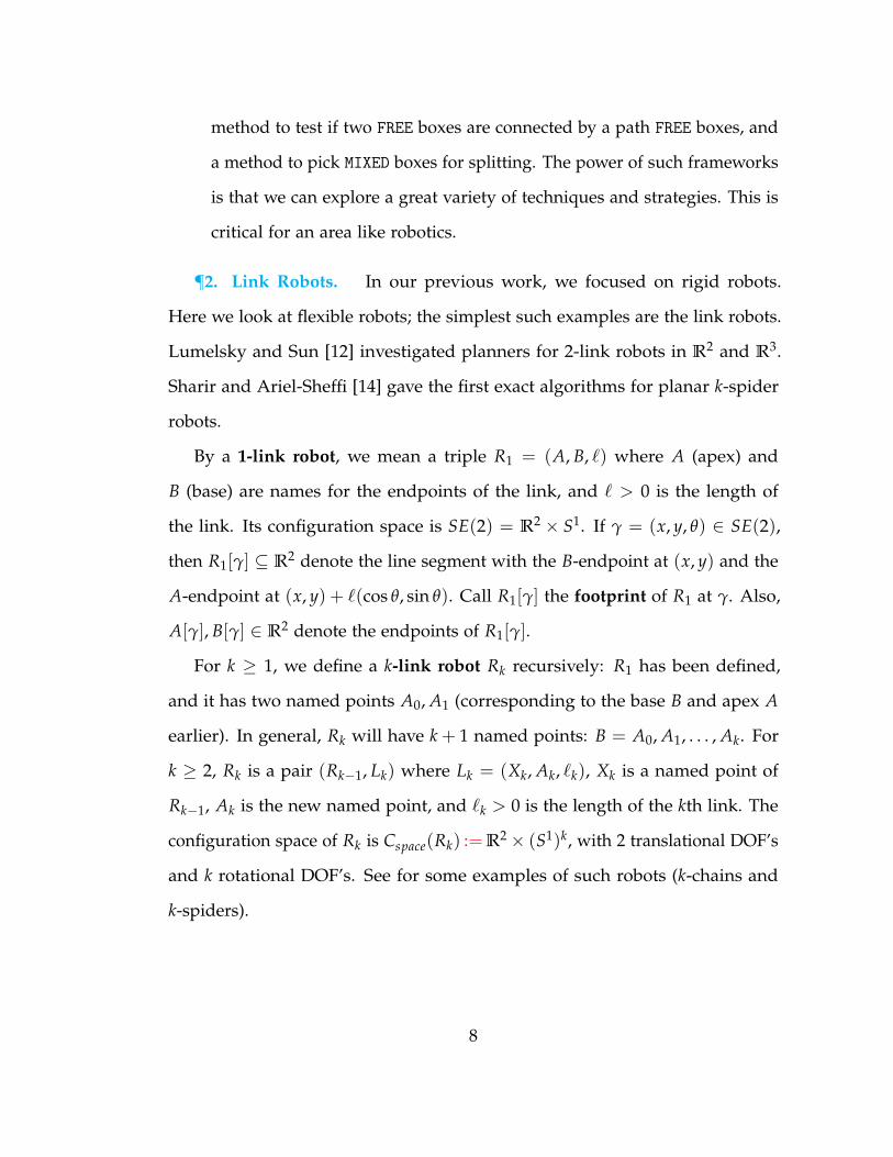
For k ≥ 1, we define a k-link robot Rk recursively: R1 has been defined,

and it has two named points A0, A1 (corresponding to the base B and apex A

earlier). In general, Rk will have k + 1 named points: B = A0, A1, . . . , Ak. For

k ≥ 2, Rk is a pair (Rk−1, Lk) where Lk = (Xk, Ak, `k), Xk is a named point of

Rk−1, Ak is the new named point, and `k > 0 is the length of the kth link. The

configuration space of Rk is Cspace(Rk) :=R2× (S1)k, with 2 translational DOF’s

and k rotational DOF’s. See for some examples of such robots (k-chains and

k-spiders).

8

Figure 2.1: Some link robots

We define the footprint of Rk: Let γ = (γ′, θk) ∈ Cspace(Rk) where γ′ =

(x, y, θ1, . . . , θk−1). The footprint of the kth link is Lk[γ], defined as the line

segment with endpoints Xk[γ′] and Ak[γ] := Xk[γ

′] + `k(cos θk, sin θk). The foot-

print Rk[γ] is the union Rk−1[γ′] ∪ Lk[γ].

We say γ is free if Rk[γ]∩Ω = ∅. As usual, C f ree(Rk) ⊆ Cspace(Rk) comprise

the free configurations. The clearance of γ is defined as C`(γ) := Sep(Rk[γ], Ω).

Here, Sep(X, Y) := inf ‖x− y‖ : x ∈ X, y ∈ Y denotes the separation of two

Euclidean sets X, Y ⊆ R2.

¶3. Features-Based Approach. Our computation and predicates are "fea-

ture based" whereby the evaluation of box primitives are based on a set φ(B) of

features associated with the box B.

Given a polygonal set Ω ⊆ R2, the boundary ∂Ω may be subdivided into

a unique set of corners (points) and edges (open line segments), called the

features of Ω. Let Φ(Ω) denote this feature set. Our representation of f ∈ Φ(Ω)

ensures this local property of f : for any point q, if f is the closest feature to q, then

we can decide if q is inside Ω or not. To see this, first note that if f is a corner, then

q must be outside Ω. So suppose f is a wall. Our representation assigns an

9

orientation to f such that q is inside Ω iff q lies to the left of of the oriented line

through f .

10

Chapter 3

The T/R Splitting Method

The simplest splitting strategy is to split a box B ⊆ Rd into 2d congruent

subboxes. This makes sense for a disc robot, but even for the case of Cspace =

SE(2), this strategy is noticeably slow without additional techniques. In [16],

The splitting of rotational dimensions is delayed, but the problem of 23 = 8

splits eventually shows up. Here, let’s push the delaying idea to the limit: we

would like to split the rotational dimensions only once, at the leaves of the subdivision

tree when the translational boxes have radius at most ε. Moreover, this rotational

split can produce arbitrarily many children, depending the number of relevant

obstacle features. Intuitively, reducing the translational box down to ε for

this technique is not severely inefficient because there are only a 2 DOF for

translation. Later, we introduce a modification.

The basis for this approach is a distinction between the translational and rota-

tional components of Cspace. Note that the rotational component is a subspace of

a compact space (S1)k, and thus it makes sense to treat it differently. Given a box

B ⊆ Cspace(Rk), we write B = Bt× Br where Bt ⊆ R2 and Br ⊆ (S1)k are (respec-

tively) the translational box (t-box) and rotational box (r-box) corresponding

11

to B.

For any box B ⊆ Cspace(Rk), let its midpoint mB = m(B) and radius rB =

r(B) refer to the midpoint and radius of its translation part, Bt. Suppose the

rotational part of B is given by Br = ∏ki=1[θi ± δ].

Suppose we want to compute a soft predicate C(B) to classify boxes B ⊆

Cspace(Rk). Following our previous work [16, 17], we reduce this to computing

a feature set φ(B) ⊆ Φ(Ω). The feature set φ(B) of B is defined as comprising

those features f such that Sep(mB, f ) ≤ rB + r0 where r0 is farthest reach of the

robot links from its base (i.e., A0).

We say B is empty if φ(B) is empty but φ(B1) is not, where B1 is the parent

of B. We may assume the root is never empty. If B is empty, it is easy to decide

whether B is FREE or STUCK: since the feature set φ(B1) is non-empty, we can

find the f1 ∈ φ(B1) such that Sep(mB, f1) is minimized. Then Sep(mB, f1) > rB,

and by the above local property of features, we can decide if mB is inside or

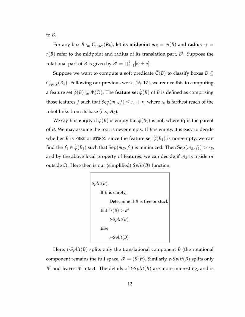
outside Ω. Here then is our (simplified) Split(B) function:

Split(B):

If B is empty,

Determine if B is free or stuck

Elif “r(B) > ε”

t-Split(B)

Else

r-Split(B)

Here, t-Split(B) splits only the translational component B (the rotational

component remains the full space, Br = (S1)k). Similarly, r-Split(B) splits only

Br and leaves Bt intact. The details of t-Split(B) are more interesting, and is

12

taken up in the next chapter.

¶4. Modified T/R Strategy. A possible modification to this T/R strategy is

to replace the criterion “r(B) > ε” of Split(B) by “r(B) > ε and |φ(B)| ≥ c”, for

some (small) constant c. For instance if |φ(B)| = 2, we might be in a corridor

region and it seems a good idea to start to split the angles. The problem with

this variation is that the r-Split(B) gives only an approximation of the possible

rotational freedom in B; if no path is found, we may have to split Bt again, in

order to apply r-Split to the children of B. This may render it slower than the

simple T/R strategy. As our experiments show, a choice like c = 4 is a good

default.

13

Chapter 4

Soft Predicate for Rotational Degrees of Free-

dom

We design the rotational r-Split(B) routine. Recall that this amounts to splitting

Br but leaving Bt intact. We first assume simple case where Rk is a k-spider. In

this case, each link of the robot is independent, so it suffices to consider the case

of one link (R1). For simplicity, assume Br = S1. If this link has length ` > 0,

then r-Split(B) splits the full circle S1 into a union of free angular intervals. The

number of such free angular ranges is equal to the number of features in φ(B)

within distance ` from m(B).

Use the following convention for closed angular ranges: if 0 ≤ α1 < α2 < 2π,

then let

[α1, α2] := α : α1 ≤ α ≤ α2 and [α2, α1] := α : 0 ≤ α ≤ α1 or α2 ≤ α < 2π. In

any case, if [α, α′] is an angular range, we call α (resp., α′) the left stop (resp.,

right stop) of the angular range.

14

Figure 4.1: Example of a t-Split process

Figure 4.2: Common tangent rays method used in r-Split

For s, t ∈ R2, let Ray(s, t) denote the ray originating at s and passing through

t, and let θ(s, t) ∈ [0, 2π) = S1 denote its orientation. As usual, let the positive

x- and y-axes have orientations 0 and π/2, respectively. If S, T ⊆ R2 are sets,

let Ray(S, T) = Ray(s, t) : s ∈ S, t ∈ T. For ` > 0, define length-limited (or

15

`-limited) forbidden range of S, T to be

Forb`(S, T) := θ(s, t) : s ∈ S, t ∈ T, ‖s− t‖ ≤ ` .

If S ∩ T is non-empty, then Forb`(S, T) = S1. Hence we will assume S ∩ T = ∅.

We may also assume S, T are closed convex sets. To understand this forbidden

range, we initially set ` = ∞, and simply write Forb(S, T) for Forb∞(S, T). Call

Ray(s, t) ∈ Ray(S, T) a common tangent ray if the line through Ray(s, t) is

tangential to S and to T. Such a ray is separating if S and T lie on different

sides of the line through Ray(s, t). If S, T are not singletons, then there are

four common tangent rays, and exactly two of them are separating. We call

a separating common tangent ray a left stop (resp., a right stop) of (S, T) if

S lies to the right (resp., left) of the ray. Now it can be verified that θ(S, T) =

[θ(s1, t1), θ(s2, t2)] where Ray(s1, t1) and Ray(s2, t2) are the left and right stops

of (S, T), as illustrated in Figure 4.2.

Figure 4.3: Forbidden Range Forb(B, W) between box B and wall W

16

We apply these observations to the case where S is a translational box Bt and

T is a wall W. If s is a side of Bt, let H(s) denote the closed half-space bounded

by s and that has empty intersection with the interior of Bt. Up to symmetry,

there are three cases as seen in Figure 4.3:

(I) Bt has a side s such that W ⊆ H(s).

(II) Bt has two consecutive sides s and s′ such that W ⊆ H(s) ∩ H(s′).

(III) Bt has two consecutive sides s and s′ such that W crosses H(s) ∩ H(s′).

We can now easily compute the forbidden range (refer to Figure 4.3):

Forb(Bt, W) =

[θ(v, C), θ(v′, C′)] if Case (Ia) or (IIa),

[θ(v, C), θ(v′, C)] if Case (Ib) or (IIb),

[θ(v, C), θ(v, C′)] if Case (III).

(4.1)

Then we shall advance to the length-limited forbidden range.

Our goal is to determine Forb`(Bt, W) where Bt is a translational box and

W a wall. We may assume that W does not intersects Bt, because otherwise

Forb`(Bt, W) = S1. It does not appear easy to convincingly enumerate the

full range of possibilities for Forb`(Bt, W) without insight. The first idea as

discussed in the text is to focus on the sets Forb(Bt, W) which is not `-limited.

In this appendix, we extend this analysis by decomposing such sets into simpler

ones for which the introduction of ` is easy to analyze. This is captured by the

following lemma:

Lemma 1. The set of `-limited forbidden angles Forb`(Bt, W) can be expressed as the

union of at most three sets of the form

17

• Forb`(v, W) where v is a corner vertex of Bt, or

• Forb`(s, C) where s is a side of Bt and C is a corner of W.

Proof. We use the cases in the formula (4.1) for Forb(Bt, W) (please refer to

Figure 4.3 for notation):

CASE (I) In CASE (I), the wall W lies in the half-space H(s) for some side s

of Bt. We now characterize the distinction between SUBCASES (Ia) and

(Ib): let z denote the intersection of the line through W and line through

s. If z lies outside s, then we are in SUBCASE (Ia); otherwise we are in

SUBCASE (Ib). The situation where z is undefined because W and s are

parallel will be treated under SUBCASE (Ia) below.

First consider SUBCASE (Ia) where C, C′ are distinct corners of W. Note

that Forb(Bt, W) = [θ(v, C), θ(v′, C′)] can be written as the union of two

angular ranges,

Forb(Bt, W) = Forb(s, C′) ∪ Forb(v, W). (4.2)

But it could also be written as

Forb(Bt, W) = Forb(s, C) ∪ Forb(v′, W). (4.3)

How should we choose between these two representations of Forb(Bt, W)?

Recall that SUBCASE (Ia) is characterized by the fact that intersection

point z lies outside s; wlog, assume that z lies to the left of s as in .

18

Figure 4.4: Length-limited Forbidden Zone Analysis

Suppose α ∈ Forb(Bt, W). Then (4.2) implies that there exists a pair

(a, b) ∈ (s× C′) ∪ (v×W)

such that θ(a, b) = α. Similarly, (4.2) implies that there exists a pair

(a′, b′) ∈ (s× C) ∪ (v′ ×W)

such that θ(a, b) = α. One such angle is illustrated in with (a, b) = (v, b)

and (a′, b′) = (a′, C).

It is not hard to verify that the geometry of this subcase implies

‖a− b‖ ≤ ‖a′ − b′‖.

It follows that

α ∈ Forb`(Bt, W)⇐⇒ α ∈ Forb`(s, C′) ∪ Forb`(v, W).

19

In other words, the representation (4.2) (not (4.3)) extends to the `-limited

forbidden angles:

Forb`(Bt, W) = Forb`(s, C′) ∪ Forb`(v, W). (4.4)

Note that in case W and s are parallel, both representations (4.2) and (4.3)

are equally valid.

It remains to treat SUBCASE (Ib), we have C = C′ and so the preceding

argument reduces to Forb`(Bt, W) = Forb`(C, s).

CASE (II) First consider SUBCASE (IIa) where C, C′ are distinct corners of W.

The analysis of CASE (Ia) can be applied twice to this case, yielding

Forb`(Bt, W) = Forb`(v, W) ∪ Forb`(s, C′) ∪ Forb`(s′, C′). (4.5)

For SUBCASE (IIb), we have C = C′ and so Forb`(v, W) can be omitted.

Thus Forb`(Bt, W) = Forb`(s, C) ∪ Forb`(s′, C).

CASE (III) This is simply

Forb`(Bt, W) = Forb`(v, W). (4.6)

Q.E.D.

This lemma shows how to reduce Forb`(B, W) to the special cases of Forb`(v, W)

and Forb`(s, C). It remains to show how to determine these sets. But this is

20

easy: if D`(v) denotes the disc centered at v of radius `, then

Forb`(v, W) = Forb(v, D`(v) ∩W),

Forb`(s, C) = Forb(D`(C) ∩ s, C).

This concludes our analysis of Forb`(B, W). The proof of our lemma also contain

the necessary information for implementing Forb`(B, W).

Now we are ready to describe the r-Split(B) operator: Consider the set

S1 \(⋃

i Forb`(Bt, Wi))

where Wi range over all walls with at least one corner in

φ(B). Write this set as the union of disjoint angular ranges

Θ(B) := A1 ∪ A2 ∪ · · · ∪ Ak. (4.7)

Then r-Split(B) returns the set of boxes Bt × Ai (for i = 1, . . . , k). The union of

these boxes is denoted⋃

r-Split(B).

We address correctness of this method. The following lemma is about

convergence and effectivity. Clearly,⋃

r-Split(B) ⊆ B ∩ C f ree. But how good

is⋃

r-Split(B) as an approximation of B ∩ C f ree? This is the question about

effectivity of our approximation, and is answered in part(ii) of this lemma.

Lemma 2.

(i) Let (B1, B2, . . .) be a sequence of boxes in Cspace where Bi = Bti × S1, and Bt

i

converges to a point p as i→ ∞. Then⋃

r-Split(Bi) converges to the set (p× S1) ∩

C f ree, i.e., the free configurations with the base at p.

(ii) Let B = Bt × S1. If γ ∈ B has clearance C`(γ) > 2 · r(B), then γ ∈ ⋃ r-Split(B)

Proof. (i) is immediate. To see (ii), let γ = (p, θ) ∈ B. We prove the

contra-positive. Suppose γ /∈ ⋃ r-Split(B). Then there is some p′ ∈ Bt such

21

that γ′ = (p′, θ) is not free. But Sep(R1[γ], R1[γ′]) ≤ 2 · r(Bt). This implies

C`(γ) ≤ 2 · r(Bt) = 2 · r(B). Q.E.D.

Theorem 3. Assume the T/R method for splitting and r-Split is implemented exactly

in our SSS Algorithm for a spider robot Rk. Then we obtain an resolution-exact planner

for Rk.

The proof follows the general approach in [16, 18]. Of course, we have no

intention of implementing r-Split exactly. Instead, if we implement r-Split(B)

using a conservative approximation with absolute error bounded by r(B), then

we obtain a corresponding resolution-exact algorithm (but with larger constant

K).

22

Chapter 5

Experimental Results

We have implemented in C/C++ the planner for 2-link robots as described in this

paper. The experiments are conducted on a laptop with OSX 10.8, Intel Core

i7-3610QM CPU and 8GB of RAM.

Our source code and datasets are freely distributed with the Core Library1.

The parameter settings for our experiments on a variety of obstacle inputs

are encoded as targets in a Makefile. Thus users can easily reproduce our

results and conduct further experiments. Here we show the performance on our

example targets. Each obstacle set is stored in own text file, and is represented

by a set of polygons (not necessarily disjoint) in a square of dimension 512 x

512. Most of the obstacles sets were specially designed for their interest and

challenge for our planners. For instance, eg5 involves a double bugtrap and

eg300 involves 300 triangles generated at random. Images of our obstacle sets

are shown in Figs. 1-7 in the Appendix.

For each obstacle set, Table 5.1 shows two statistics from running our planner:

total running time and the total number of tree boxes created. Each run has the

1http://cs.nyu.edu/exact/core/download/core/.

23

parameters (`1, `2, S, ε, x1, y1, α1, α2, x2, y2, β1, β2) where `1, `2 are the lengths of

the 2 links, S ∈ B, D, G indicates2 the search strategy (B = Breadth First Search

(BFS), D = Distance + Size, G = Greedy Best First (GBF)), (x1, y1, α1, α2) is the

start configuration and (x2, y2, β1, β2) is the goal configuration. In Table 5.1,

we pick two variants of T/R splitting: “Simple T/R” means applying r-Split

when the box size is < ε, and “Modified T/R” means applying r-Split when

the feature set size is small enough (controlled by the parameter c mentioned

at the end of Section 3). The choice c = 4 is used here. We see that GBF and

“Distance + Size” are comparable to each other, and always faster than BFS.

Obstacle Set robot Modified T/R (c = 4) Simple T/R Performance(x1, y1, α1, α2, x2, y2, β1, β2) (`1, `2, S, ε) time (ms) boxes time (ms) boxes Improvementeg1 (50,80,G,4) 155.6 8232 158.8 8514 2.0%(Barrier Environment) (50,80,D,4) 175.3 10886 176.7 10042 0.8%(195,340,0,150,260,80,70,120) (50,80,B,4) 413.1 29615 403.0 28802 -9.3%

(20,10,G,4) 25.9 2604 30.3 3985 14.5%eg2 (85,80,G,4) 372.8 23803 482.6 33199 -22.7%(8-way corridor) (85,80,D,4) 318.6 21400 316.4 20060 -0.7%(216,297,115,155,210,220,260,200) (85,80,B,4) 577.8 53393 485.4 48851 -19.0%eg3 (100,70,G,4) 163.5 12530 165.7 12530 1.3%(8 ways) (100,70,D,4) 136.7 12005 135.4 12005 -0.9%(262,250,180,270,271,256,90,0) (100,70,B,4) 269.0 21529 274.9 21529 2.1%eg5 (60,50,G,4) 559.1 22781 532.5 22617 -5.0%(Double Bugtrap) (60,50,D,4) 625.3 25007 645.1 27185 3.1%(190,210,180,300,30,30,90,0) (60,50,B,4) 684.0 40007 687.9 39868 0.6%

(20,20,G,4) 107.5 7637 122.3 10858 12.1%eg10 (65,80,G,4) 99.1 9068 100.8 9068 1.7%(2 Chambers) (65,80,D,4) 74.6 7416 75.3 7416 0.9%(425,410,180,270,105,90,90,0) (65,80,B,4) 151.8 15627 147.7 15627 -2.8%eg300 (40,30,G,4) 205.6 6132 201.4 6133 -2.1%(300 Triangles) (40,30,D,4) 201.5 6376 201.8 6337 0.1%(10,400,90,270,330,40,270,0) (40,30,B,4) 2657.3 52318 2414.1 49944 -10.1%

Table 5.1: Statistics of running our algorithms with ε = 4

In Table 5.2, we fix the other configurations and try to compare the cases with

different ε. We can see when ε gets smaller, more splits are generated and the

2Note that a random strategy is never competitive.

24

calculation gets much slower. According to the result, when we halve ε, we get

nearly 2X-6X more boxes. It fits the quadruple ratio from translational splittings.

The ratio may get worse in Modified T/R since it may suffer a lot by doing

useless rotational splittings.

Obstacle Set Robot Modified T/R (c = 4) Simple T/R Ratio by Boxes(x1, y1, α1, α2, x2, y2, β1, β2) (`1, `2, S, ε) time (ms) boxes time (ms) boxes (using ε=1 as base)eg1 (50,80,D,4) 175.3 10886 176.7 10042 39.22 12.67(Barrier Environment) (50,80,D,2) 958.1 71596 651.0 35229 5.96 3.61(195,340,0,150,260,80,70,120) (50,80,D,1) 5293.2 426975 2506.2 127265 1.0 1.0eg2 (85,80,D,4) 335.4 21400 323.4 20060 7.99 8.52(8-way corridor) (85,80,D,2) 624.0 47662 623.9 47662 3.59 3.59(216,297,115,155,210,220,260,200) (85,80,D,1) 2234.2 170901 2225.0 170901 1.0 1.0eg3 (100,70,D,4) 136.7 12005 135.4 12005 19.49 19.49(8 ways) (100,70,D,2) 591.5 55227 588.6 55227 4.24 4.24(262,250,180,270,271,256,90,0) (100,70,D,1) 2505.9 233951 1460.0 233951 1.0 1.0eg5 (60,50,D,4) 625.3 25007 645.1 27185 35.66 15.63(Double Bugtrap) (60,50,D,2) 2432.1 102984 2517.2 107113 8.66 3.97(190,210,180,300,30,30,90,0) (60,50,D,1) 17497.7 891809 9740.9 425011 1.0 1.0eg10 (65,80,D,4) 74.6 7416 75.3 7416 14.94 14.94(2 Chambers) (65,80,D,2) 300.3 29165 299.7 29165 3.80 3.80(425,410,180,270,105,90,90,0) (65,80,D,1) 1212.3 110779 1198.2 110771 1.0 1.0eg12 (45,45,D,4) 363.9 17375 359.3 17494 16.10 14.33(Maze) (45,45,D,2) 1288.8 65979 1304.4 65751 4.24 3,81(405,400,180,270,105,60,0,180) (45,45,D,1) 5341.7 279818 4972.4 250772 1.0 1.0eg300 (40,30,D,4) 201.5 6376 201.8 6337 11.56 11.60(300 Triangles) (40,30,D,2) 594.5 19304 573.7 19273 3.82 3.81(10,400,90,270,330,40,270,0) (40,30,D,1) 2223.0 73719 2240.5 73509 1.0 1.0

Table 5.2: Statistics of running our algorithms with different ε

In Table 5.3, we compare the configurations with different c from 1 to 6. Accord-

ing to the result, the best c may vary. It’s hard to get a constant suitable c for

each case.

25

Obstacle Set Robot Modified T/R Simple T/R(x1, y1, α1, α2, x2, y2, β1, β2) (`1, `2, S, ε, c) time (ms) boxes time (ms) boxeseg1 (50,80,D,4,1) 173.0 10042 176.7 10042(Barrier Environment) (50,80,D,4,2) 178.8 10042 - -(195,340,0,150,260,80,70,120) (50,80,D,4,3) 174.8 10269 - -

(50,80,D,4,4) 175.3 10886 - -(50,80,D,4,5) 199.6 11773 - -(50,80,D,4,6) 294.7 17220 - -

eg2 (85,80,D,4,1) 299.2 20060 300.4 20060(8-way corridor) (85,80,D,4,2) 301.5 20100 - -(216,297,115,155,210,220,260,200) (85,80,D,4,3) 305.0 20576 - -

(85,80,D,4,4) 318.6 21400 - -(85,80,D,4,5) 347.0 24017 - -(85,80,D,4,6) 330.1 23717 - -

eg3 (100,70,D,4,1) 137.4 12005 135.4 12005(8 ways) (100,70,D,4,2) 137.5 12005 - -(262,250,180,270,271,256,90,0) (100,70,D,4,3) 136.8 12005 - -

(100,70,D,4,4) 136.7 12005 - -(100,70,D,4,5) 136.9 12005 - -(100,70,D,4,6) 137.4 12005 - -

eg5 (60,50,D,4,1) 620.9 26790 645.1 27185(Double Bugtrap) (60,50,D,4,2) 628.9 26617 - -(190,210,180,300,30,30,90,0) (60,50,D,4,3) 619.0 25384 - -

(60,50,D,4,4) 625.3 25007 - -(60,50,D,4,5) 619.9 25101 - -(60,50,D,4,6) 731.7 34662 - -

eg10 (65,80,D,4,1) 73.6 7416 75.3 7416(2 Chambers) (65,80,D,4,2) 74.0 7416 - -(425,410,180,270,105,90,90,0) (65,80,D,4,3) 73.4 7416 - -

(65,80,D,4,4) 74.6 7416 - -(65,80,D,4,5) 74.5 7416 - -(65,80,D,4,6) 78.6 7948 - -

eg12 (45,45,D,4,1) 359.3 17494 359.3 17494(Maze) (45,45,D,4,2) 358.6 17376 - -(405,400,180,270,105,60,0,180) (45,45,D,4,3) 357.7 17352 - -

(45,45,D,4,4) 363.9 17375 - -(45,45,D,4,5) 361.0 17383 - -(45,45,D,4,6) 356.3 17338 - -

eg300 (40,30,D,4,1) 195.7 6337 201.8 6337(300 Triangles) (40,30,D,4,2) 194.9 6337 - -(10,400,90,270,330,40,270,0) (40,30,D,4,3) 195.5 6376 - -

(40,30,D,4,4) 201.5 6376 - -(40,30,D,4,5) 195.3 6393 - -(40,30,D,4,6) 192.5 6311 - -

Table 5.3: Statistics of running our algorithms with different c

26

Chapter 6

Non-Crossing 2-Link Robot

In this chapter we analyze a special kind of 2-link robot called Non-Crossing

robot. To introduce this concept, we address the following phenomena at first:

in the screen shot of Figure 6.1, we show two configurations of the 2-link robot

inside an (inverted) T-room environment. Let α (respectively, β) be the start

(goal) configuration as indicated1 by the double (single) circle. There are obvious

paths from α to β whereby the robot origin moves directly from the start to goal

positions and simultaneously, the link angles monotonically adjust themselves,

as illustrated in Figure 6.3(a). However, such paths require the two links to cross

each other. To achieve a “non-crossing” path from α to β, the robot origin must

initially move away from the goal configuration towards the T-junction first, in

order to maneuver the two links into the appropriate relative order before it

can move toward the goal configuration. Such a non-crossing path is shown

in Figure 6.3(b). We find such paths with a subdivision algorithm; Figure 6.2

illustrates the subdivision of the underlying configuration space (the scheme is

explained below).

1Our images have color: the double circle is cyan and single circle is magenta. The robotlinks are colored blue (`1) and red (`2), respectively.

27

Figure 6.1: T-Room: start and goal configurations

Figure 6.2: T-room: Subdivision

Here we show how to construct a practical and theoretically-sound planner

for a non-crossing 2-link robot. Our planner may (but not always) suffer a

loss of efficiency when compared to the self-crossing 2-link planner (see [13]).

Nevertheless, it gives real-time performance for a variety of non-trivial obstacle

environments such as illustrated in Figure 6.4 (200 randomly generated trian-

gles), Figure 6.5(a) (Double Bug-trap (cf. [p. 181, Figure 5.13][11]), Figure 6.5(b)

(Maze).

For example, Figure 6.4(a) is an environment with 200 randomly generated

28

Figure 6.3: T-room: Left side is the self-crossing solution, Right side is the non-crossingsolution.

triangles, and a path is found with ε = 4. If we use ε = 5, then it returns

NO-PATH as shown in Figure 6.4(b). This NO-PATH declaration guarantees

that there is no path with clearance > Kε (for some constant K).

6.1 Configuration Space of Non-Crossing Robot.

The self-crossing configuration space of R2 is

Cspace = R2 × T (6.1)

where T = S1 × S1 is the torus. The configuration of link robots is treated in

Devadoss and O’Rourke [5, chap. 7]. Consider a configuration γ = (x, y, θ1, θ2) ∈

Cspace where θi (i = 1, 2) is the orientation of the i-th link (see Figure 2.1(a)).

When θ1 = θ2, we say the configuration is self-crossing; otherwise it is non-

crossing. Let

∆ :=(θ, θ) : θ ∈ S1

, T∆ := T \ ∆.

29

Figure 6.4: 200 Random Triangles.

Also, let T< := (θ, θ′) ∈ T : θ < θ′ and T> := (θ, θ′) ∈ T : θ > θ′. We are

interested in planning the motion of R2 in the non-crossing configuration

space,

C∆space :=R2 × T∆. (6.2)

Note that ∆ is a closed curve in T . In R2, a closed curve will disconnect the

plane into two connected components. But the curve ∆ does not disconnect

T . To see this, consider the plane model of T represented by a square with

opposite sides identified as shown in Figure 6.6. Each of the sets T< and T> are

themselves connected; moreover, any α ∈ T> and β ∈ T< are path-connected in

T∆ (as illustrated in Figure 6.6).

Let us be specific about how to interpret the parameters of Cspace. The robot

R2 has three named points A0, A1, A2 (see [13]), shown in Figure 2.1(a), where

A0 is the robot joint (or origin).The footprint of these points at a configuration

30

Figure 6.5: (a) Double Bugtrap, (b) Maze.

γ = (x, y, θ1, θ2) are given by

A0[γ] := (x, y),

A1[γ] := (x, y) + `1(cos θ1, sin θ1),

A2[γ] := (x, y) + `2(cos θ2, sin θ2).

Let R2[γ] ⊆ R2 denote the footprint of R2 at γ, defined as the union of the line

segments [A0[γ], A1[γ]] and [A0[γ], A2[γ]].

6.2 Subdivision for Non-Crossing 2-Link Robot

Suppose we already have a resolution-exact planner for a self-crossing 2-Link

robot. We now describe a simple transformation to convert it into a resolution-

exact planner for a non-crossing 2-Link robot.

31

Figure 6.6: Paths in T∆ from α ∈ T> to β ∈ T<

6.2.1 Subdivision of Boxes

In this paper, we are interested in a slight generalization of such boxes.

By a box (or d-box) of dimension d ≥ 1 we mean a set of the form B = ∏di=1 Ii

where d ≥ 1 and each Ii is a closed interval of R or S1 of positive length. Such

boxes are natural for doing subdivision in configuration spaces of the form

Rk × (S1)d−k. For our 2-link robots, d = 4 and k = 2. The configuration space

for a submarine or helicopter might be regarded as R3 × S1.

For i = 1, . . . , d, we have the notion of i-projection and i-coprojection of

d-boxes:

• (Projection) Proji(B) := ∏dj=1,j 6=i Ij is a (d− 1) dimensional box.

• (Co-Projection) Coproji(B) := Ii is the ith interval of B.

We also define the indexed Cartesian product ⊗i via the identity

B = Proji(B)⊗i Coproji(B).

Let j = −1, 0, 1, . . . , d. Two boxes B, B′ of dimension d ≥ 1 are said to be

32

j-adjacent if dim(B ∩ B′) = j. Note that B and B′ are (−1)-adjacent means they

are disjoint. When i = d− 1, we simply say the boxes are adjacent, denoted

B :: B′; when i = d, we say they are overlapping, denoted B B′. The following

is immediate:

Lemma 4. Let B, B′ be boxes of dimension d ≥ 1.

• If d = 1 then B :: B′ iff |B ∩ B′| ∈ 1, 2.

• If d > 1 then B :: B′ iff (∃i = 1, . . . , d) such that

Proji(B) Proji(B) ∧ Coproji(B) :: Coproji(B′).

6.2.2 Boxes for Non-Crossing Robot.

Our basic idea for representing boxes in the non-crossing configuration space

C∆space is to write it as a pair (B, XT) where XT ∈ LT, GT, and B is a box in

self-crossing configuration space Cspace. The pair (B, XT) represents the set

B ∩ (R2× TXT) (with the identification TLT = T< and TGT = T>). It is convenient

to call (B, XT) an X-box since they are no longer “boxes” in the usual sense.

As in [13], we may write B as the Cartesian product of a translational box

Bt and a rotational box Br: B = Bt × Br where Bt ⊆ R2 and Br ⊆ T . Thus,

Br = Θ1 × Θ2 where Θ1, Θ2 ⊆ S1 are angular intervals. We denote (closed)

angular intervals by [s, t] where s, t ∈ [0, 2π] and using the interpretation

[s, t] :=

θ : s ≤ θ ≤ t if s < t,

[s, 2π] ∪ [0, t] if s ≥ t.

33

In particular, [s, s] = [s, t] ∪ [t, s] = S1. An angular interval [s, t] that2 contains

a neighborhood of 0 = 2π is said to be wrapping. Also, call Br = Θ1 × Θ2

wrapping if either Θ1 or Θ2 is wrapping.

Given any Br, we can decompose the set Br ∩T∆ into the union of two subsets

BrLT and Br

GT, where BrXT denote the set Br ∩ TXT. In case Br is non-wrapping, this

decomposition has the nice property that each subset BrXT is connected. For this

reason, we prefer to work with non-wrapping boxes. Initially, the box Br = T is

wrapping. The initial split of T should be done in such a way that the children

are all non-wrapping: the “natural” (quadtree-like) way to split T into four

congruent children has3 this property. Thereafter, subsequent splitting of these

non-wrapping boxes will remain non-wrapping.

Of course, BrXT might be empty, and this is easily checked: say Θi = [si, ti]

(i = 1, 2). Then Br< is empty iff t2 ≤ s1. and Br

> is empty iff s2 ≥ t1. Moreover,

these two conditions are mutually exclusive.

We now modify the algorithm of [13] as follows: as long as we are just

splitting boxes in the translational dimensions, there is no difference. When

we decide to split the rotational dimensions, we use the T/R splitting method

of [13], but each child is further split into two X-boxes annotated by LT or

GT (they are filtered out if empty). We build the connectivity graph G (see

Appendix 2) with these X-boxes as nodes. This ensures that we only find non-

crossing paths. Our algorithm inherits resolution-exactness from the original

self-crossing algorithm.

2Wrapping intervals are either equal to S1 or has the form [s, t] where s > t, s 6= 2π andt 6= 0

3This is not a vacuous remark – the quadtree-like split is determined by the choice of a“center” for splitting. To ensure non-wrapping children, this center is necessarily (0, 0) orequivalently (2π, 2π). Furthermore, our T/R splitting method (to be introduced) does notfollow the conventional quadtree-like subdivision at all.

34

6.3 Extension to Diagonal Band

The diagonal ∆ is a curve with no width. We now want to fatten ∆ into a band

∆(κ) of bandwidth κ ≥ 0. For this extension, we use the intrinsic Riemannian

metric on S1: the distance between θ, θ′ ∈ S1 is given by

d(θ, θ′) = min|θ − θ′|, 2π − |θ − θ′|

.

where we may assume θ, θ′ ∈ [0, 2π]. Fix 0 ≤ κ < π. Then

∆(κ) :=(θ, θ′) ∈ T : d(θ, θ′) ≤ κ

.

Thus the original diagonal line is ∆(0) = ∆. The non-crossing configuration

space is now

C∆(κ)space = R2 × (T \ ∆(κ)).

This extension is very useful in applications. For example, the T-room example

(Figures 6.1–6.2) uses κ = 10. Moreover, if we set κ = 11, then there is

NO-PATH. It is not surprising that as κ is increased, we may no longer be able

to find a path. But somewhat surprisingly, our experiments (see Table I below)

show that increasing κ may also speed up the search for a path.

The predicate isBoxEmpty(Br, κ, XT) which returns true iff (BrXT) ∩ T∆(κ) is

empty is useful in implementation. It has a simple expression when restricted

to non-wrapping translational box Br:

Lemma 5.

Let Br = [a, b]× [a′, b′] be a non-wrapping box.

35

(a) isBoxEmpty(Br, κ, LT) = true iff κ ≥ b′ − a or 2π − κ ≤ a′ − b.

(b) isBoxEmpty(Br, κ, GT) = true iff κ ≥ b− a′ or 2π − κ ≤ a− b′.

6.4 Implementation and Experiments

Our current implementation is based on machine arithmetic, but it is relatively

straightforward to ensure arbitrary precision using bigFloat numbers and “lax

comparison” as described in [16].

Table 6.1 compares the performance of the non-crossing planner with the

original crossing planner from [13]. Each row of Table I shows two statistics for

the self-crossing and non-crossing planners: total running time and the total

number of subdivision boxes created. The last column shows the percentage

improvement in time for non-crossing over self-crossing.

We use various obstacle sets (named egX such as eg2a, eg2b, eg5, etc.).

Each run is a row in the Table, and has these parameters (`1, `2, S, ε, κ) where

`i is the length of the i-th link, S ∈ B, D, G indicates4 the search strategy

(B = Breadth First Search (BFS), D = Distance + Size, G = Greedy Best First

(GBF)). The last parameter κ ∈ [0, 180) is the bandwidth of ∆ in degrees. When

we run the self-crossing planner the κ parameter is ignored. The parameters for

each run are encoded in a Makefile.

Table 6.1 shows that the running time of the non-crossing planner is compa-

rable to that of the self-crossing planner in all the examples (with the exception

of the T-room or eg13). Their percentage change is between −44.8% to 11.4%.

That is because, although non-crossing planner has some overhead, it also filters

out useless splittings earlier for the dead ends. The exceptional case (T-room)

4A random strategy is available, but it is never competitive.

36

is explained by the fact that the non-crossing planner must use a much longer

circuitous path.

Table 6.2 shows the sensitivity of finding a path to the link length `2, and to

the bandwidth κ, as ε decreases.

Obstacle Set Configuration Self-Crossing Non-Crossing Performance(x1, y1, α1, α2, x2, y2, β1, β2) (`1, `2, S, ε, κ) time (ms) boxes time (ms) boxes Improvementeg2b (88, 98, D, 2, 79) 1740.1 104663 1591.9 71123 8.51%(8-way corridor) (88, 98, D, 2, 80) - - No Path No Path -(216,297,95,175,210,220,270,190) (88, 98, D, 2, 30) - - 1687.1 101287 3.0%

(88, 98, D, 2, 5) - - 1963.2 129394 -12.8%eg5 (55, 50, G, 4, 95) 541.2 22243 542.3 27560 -0.2%(Double Bugtrap) (55, 50, G, 4, 100) - - No Path No Path -(190,210,180,300,30,30,90,340) (55, 50, G, 4, 50) - - 613.1 32157 -13.3%

(55, 50, G, 4, 10) - - 730.3 42994 -34.9%eg8 (30, 25, G, 2, 7) 31.5 2215 45.6 5214 -44.8%(Hsu et al. [7]) (30, 25, G, 2, 8) - - No Path No Path -(20,390,0,270,275,180,270,0) (30, 25, G, 2, 3) - - 37.3 3514 -18.4%eg12 (30, 33, D, 4, 146) 314.4 19953 283.3 15167 9.9%(Maze) (30, 33, D, 4, 147) - - No Path No Path -(375,400,180,0,105,60,0,180) (30, 33, D, 4, 40) - - 360.9 22908 -14.8%

(30, 33, D, 4, 10) - - 410.2 32783 -30.5%eg13 (94, 85, D, 4, 10) 3.1 616 98.9 12212 -3090%(T-Room) (94, 85, D, 4, 11) - - No Path No Path -(275,230,251,294,252,420,294,251) (94, 85, D, 4, 5) - - 94.9 12068 -2961%eg300 (40, 30, G, 4, 127) 305.7 8794 270.8 7314 11.4%(300 Triangles) (40, 30, G, 4, 128) - - No Path No Path -(10,400,90,270,270,190,270,90) (40, 30, G, 4, 40) - - 353.6 11284 -15.7%

(40, 30, G, 4, 10) - - 348.4 12113 -14.0%

Table 6.1: Comparison between Self-Crossing and Non-Crossing.

Although our current techniques work well for this 4DOF robot, we believe

that new techniques are needed to address higher DOF’s. We are working on

robots in R3. But even in the plane, real-time performance is easily compromised.

For instance, we could clearly extend the current work to non-crossing k-spiders

for k ≥ 3, with Cspace = R2 × T k where T k = (S1)k. We expect to be achieve

real-time performance for k = 3, 4. However, it is less clear that we can do the

same with k-chain robots for k ≥ 3, crossing or non-crossing.

37

Obstacle Set Configuration Self-Crossing Non-Crossing Performance(x1, y1, α1, α2, x2, y2, β1, β2) (`1, `2, S, ε, κ) time (ms) boxes time (ms) boxes Improvementeg2a (85, 80, G, 8, 10) No Path No Path No Path No Path -(8-way corridor) (85, 80, G, 4, 10) 459.0 33199 400.9 31390 12.7%(216,297,155,115,210,220,260,200) (85, 92, G, 4, 10) No Path No Path No Path No Path -

(85, 92, G, 2, 10) 2271.8 153425 2402.3 192916 -5.7%(85, 99, G, 2, 10) No Path No Path No Path No Path -(85, 99, G, 1, 10) 5887.4 385814 6190.0 448119 -5.1%(85, 100, G, 1, 10) No Path No Path No Path No Path -

eg13 (94, 85, D, 8, 10) No Path No Path No Path No Path -(T-Room) (94, 85, D, 4, 10) 3.1 616 98.9 12212 -3090%(275,230,251,294,252,420,294,251) (94, 85, D, 4, 13) - - No Path No Path -

(94, 85, D, 2, 13) 6.2 1187 417.7 47292 -6637%(94, 85, D, 2, 14) - - No Path No Path -(94, 85, D, 1, 14) 9.8 1974 1553.7 184559 -15754%(94, 85, D, 1, 15) - - No Path No Path -

Table 6.2: (a) Eg2a shows the sensitivity to length `2 as ε changes. (b) Eg13 shows thesensitivity to bandwidth κ as ε changes.

38

Chapter 7

Conclusions

We hope that the focus on soft methods will usher in renewed interest in

theoretically sound and practical algorithms in robotics, and more generally in

Computational Geometry. Our experimental results for link robots offer hopeful

signs that this is possible.

Our basic SSS framework (like PRM) is capable of many generalizations for

motion planning. One direction is to consider multiple-query models; another is

to exploit the stuck boxes for faster termination in case of NO-PATH. Extensions

to kinodynamic planning offer a chance at practical algorithms in this important

area where no known theoretical algorithms are practical. Much theoretical and

complexity analysis remains open.

It is clear that the theory of soft subdivision methods can be generalized and

extended to many traditional problems in Computational Geometry[18]. But it

also extends to new areas that are currently untouchable by our exact compu-

tational models, especially those that are defined by non-algebraic continuous

data.

Further work:

39

• The algorithms of 2-link robot can be adapted to support k-spider robot.

• 2-link robot can be expanded to chain robot with 3 or more links. It will

need new soft predicate heuristics to design and implement.

40

Bibliography

[1] S. Basu, R. Pollack, and M.-F. Roy. Algorithms in Real Algebraic Geometry.

Algorithms and Computation in Mathematics. Springer, 2nd edition, 2006.

[2] M. Brady, J. Hollerbach, T. Johnson, T. Lozano-Perez, and M. Mason. Robot

Motion: Planning and Control. MIT Press, 1982.

[3] R. A. Brooks and T. Lozano-Perez. A subdivision algorithm in config-

uration space for findpath with rotation. In Proc. 8th Intl. Joint Conf. on

Artificial intelligence - Volume 2, pages 799–806, San Francisco, CA, USA,

1983. Morgan Kaufmann Publishers Inc.

[4] H. Choset, K. M. Lynch, S. Hutchinson, G. Kantor, W. Burgard, L. E.

Kavraki, and S. Thrun. Principles of Robot Motion: Theory, Algorithms, and

Implementations. MIT Press, Boston, 2005.

[5] S. L. Devadoss and J. O’Rourke. Discrete and Computatational Geometry.

Princeton University Press, 2011.

[6] D. Halperin, L. Kavraki, and J.-C. Latombe. Robotics. In J. E. Goodman

and J. O’Rourke, editors, Handbook of Discrete and Computational Geometry,

chapter 41, pages 755–778. CRC Press LLC, 1997.

41

[7] D. Hsu, J.-C. Latombe, and H. Kurniawati. On the probabilistic foundations

of probabilistic roadmap planning. Int’l. J. Robotics Research, 25(7):627–643,

2006.

[8] L. Kavraki, P. Švestka, C. Latombe, and M. Overmars. Probabilistic

roadmaps for path planning in high-dimensional configuration spaces.

IEEE Trans. Robotics and Automation, 12(4):566–580, 1996.

[9] J.-C. Latombe. Robot Motion Planning. Kluwer Academic Publishers, 1991.

[10] S. LaValle, M. Branicky, and S. Lindemann. On the relationship between

classical grid search and probabilistic roadmaps. Int’l. J. Robotics Research,

23(7/8):673–692, 2004.

[11] S. M. LaValle. Planning Algorithms. Cambridge University Press, Cambridge,

2006.

[12] V. Lumelsky and K. Sun. A unified methodology for motion planning with

uncertainty for 2d and 3d two-link robot arm manipulators. Int’l. J. Robotics

Research, 9:89–104, 1990.

[13] Z. Luo, Y.-J. Chiang, J.-M. Lien, and C. Yap. Resolution exact algorithms

for link robots, 2014. Submitted, 30th ACM Symp. on Comp. Geom.

Preliminary version: 23rd Fall Workshop on Comp. Geom. (FWCG), Oct

25-26, 2013. The City College of New York.

[14] M. Sharir, , and E. Ariel-Sheffi. On the piano movers’ problem: Iv. various

decomposable two-dimensional motion planning problems. NYU Robotics

Report 58, Courant Institute, New York University, 1983.

42

[15] S. Thrun, W. Burgard, and D. Fox. Probabilistic Robotics. MIT press, Cam-

bridge, MA, 2005.

[16] C. Wang, Y.-J. Chiang, and C. Yap. On Soft Predicates in Subdivision

Motion Planning. In 29th ACM Symp. on Comp. Geom. (SoCG’13), pages

349–358, 2013. Full paper was invited and submitted to Comp.Geom.: Theory

& Applic. (CGTA), Special Issue for SoCG ’13.

[17] C. Yap, V. Sharma, and J.-M. Lien. Towards Exact Numerical Voronoi dia-

grams. In 9th Proc. Int’l. Symp. of Voronoi Diagrams in Science and Engineering

(ISVD)., pages 2–16. IEEE, 2012. Invited Talk. June 27-29, 2012, Rutgers

University, NJ.

[18] C. K. Yap. Soft Subdivision Search in Motion Planning. In Proceedings,

Robotics Challenge and Vision Workshop (RCV 2013), 2013. Best Paper Award,

sponsored by Computing Community Consortium (CCC). Robotics Science

and Systems Conference (RSS 2013), Berlin, Germany, June 27, 2013. Full

paper from: http://cs.nyu.edu/exact/papers/.

[19] L. Zhang, Y. J. Kim, and D. Manocha. Efficient cell labeling and path

non-existence computation using C-obstacle query. Int’l. J. Robotics Research,

27(11–12), 2008.

43

Appendices

44

APPENDIX 1: Experimental Setup

The following figures (Figs. 1-7) show the GUI interface to our implementation.

The right hand control panel allows the user to rerun with new parameters,

replay the animation, to replay the splitting of boxes, change ε or the start and

goal configurations, choose different global search strategies, modify dimensions

of the robot, etc. Subdivision boxes can also be queried.

We have a collection of predefined environments, and for each environment,

we selected some interesting parameters and encode them as targets for a

Makefile. These targets are named “egX” where X=0,1,2, etc. The examples run

in real time, even in case of NO-PATH (a feat that would challenge sampling-

based methods). Correctness of the solution is independent of the search

strategy. The straightforward randomized strategy tend to be the slowest.

45

Figure 1: Start and goal configurations for Obstacle Set eg2.

The obstacle set has 8 big triangles forming 8-way “corridors”, plus 3 small

triangles in the center. We also show the starting and ending configurations of

the 2-link robot (enclosed in a single circle and double circles respectively).

46

Figure 2: Final subdivision for Obstacle Set eg2.

The resulting path is shown, and the leaf boxes obtained during the subdivi-

sion search for the path are displayed and color coded.

Figure 3: The eg1 dataset, “barrier”

47

Figure 4: The eg3 dataset, another version of 8-way “corridors”

Figure 5: The eg5 dataset, “double bugtrap”

48

Figure 6: The eg10 dataset, “2 chambers”

Figure 7: The eg300 dataset, which has 300 randomly generated triangles

49

APPENDIX 2: Workflow of SSS Framework

We describe the main procedure of our algorithm. See [16, 18] for more details.

Our algorithm grows a subdivision tree T (B0) rooted at B0. Each tree node

is a box), the set of children of an internal node B forms a subdivision of B.

Consequently, the leaves of T (B0) forms a subdivision of B0. The nodes of

T (B0) are classified as FREE, STUCK, or MIXED, with the requirement that (1) FREE-

nodes are subsets of C f ree(R0), (2) STUCK-nodes does not intersect C f ree(R0), (3)

the internal nodes are MIXED.

There is a natural relationship adjacency graph G(T (B0)) whose nodes are

the leaves of T (B0) and two nodes are adjacent if they share a (d− 1)-face. The

tree T (B0) stops growing the moment we discover a FREE-channel connecting

α, β, i.e., a path

(B1, B2, . . . , Bm) (1)

in the graph G(T (B0)) where α ∈ B1, β ∈ Bm and each Bi is FREE. Let

PathP(α, β) be the predicate that is true iff the FREE-channel (1) exists in

G(T (B0)). This predicate is efficiently implemented with standard techniques

involving the Union-Find data structure. If Path(α, β) holds, there are also

standard methods to extract a path in Cspace from α to β from G(T (B0)); but

here we suppress details of the Union-Find and path extraction subroutines.

50

Here is the basic SSS algorithm: let BoxT (α) denote the leaf box containing

α (similarly for BoxT (α)). Note that there are two while-loops before the MAIN

LOOP, and these keep splitting BoxT (α) and BoxT (β) until they are FREE, or

else return NO-PATH.

51

SSS Framework:

Input: Configurations α, β, tolerance ε > 0, box B0 ∈ Rd.

Initialize a subdivision tree T with root B0.

Initialize priority queue Q, graph G and union-find data structure.

1. currentBox ← BoxT

While (currentBox 6= FREE)

If radius of currentBox ≤ ε, Return(NO-PATH)

Else childrenBoxes← Split(currentBox)

For childBox ∈ childrenBoxes

If Position(α) ∈ childBox, currentBox ← childBox

startBox ← currentBox

2. currentBox ← BoxT

While (currentBox 6= FREE)

If radius of currentBox ≤ ε, Return(NO-PATH)

Else childrenBoxes← Split(currentBox)

For childBox ∈ childrenBoxes

If Position(β) ∈ childBox, currentBox ← childBox

goalBox ← currentBox

3. Add B0 into QT .

4. While (Find(startBox) 6= Find(goalBox)) / MAIN LOOP

If QT is empty, Return(NO-PATH)

currentBox ← T .GetNext() / VARIOUS STRATEGIES

childrenBoxes← Split(currentBox) / DETERMINE T/R SPLITTING

For childBox ∈ childrenBoxes

If childBox is FREE

Union childBox with its FreeNeighbors separately.

Add childBox into G.

If childBox is MIXED and radius of childBox ≤ ε

Add childBox into QT .

5. Generate a shortest path from startBox to goalBox using G.

52