5th Australasian Congress on Applied Mechanics, ACAM 2007 10-12 December 2007, Brisbane, Australia

Residual Stress Measurement by Electronic Speckle Pattern Interferometry O. �edivý1, C. Krempaszky2, S. Holý1

1Department of Mechanics, Biomechanics and Mechatronics, Faculty of Mechanical Engineering,

Czech Technical University in Prague, Prague, Czech Republic 2Christian Doppler Laboratory of Material Mechanics of High Performance Alloys, Lehrstuhl für

Werkstoffkunde und Werkstoffmechanik, Technische Universität München, Garching, Germany

Abstract: The existence of residual stresses affects both safety and lifetime. Thus the determination of these stresses is very important. The ESPI (Electronic Speckle Pattern Interferometry) and Hole-Drilling combined method seems to be an appropriate technique for their measurement. The theoretical considerations about the applicability of this method based on computations and preliminary experiments are presented. The experiments on specimens simulating known residual stress distributions were carried out on a professional apparatus. These results were compared and are in good accordance with other conventional methods. The proposed technique can be used for residual stress measurements.

Keywords: electronic speckle pattern interferometry, residual stresses measurement.

1 Introduction Electronic Speckle Pattern Interferometry (ESPI) is an optical method uti lizing the speckle effect [1,2]. By comparing at least three pairs of object images all three point-displacement-components in the investigated area can be determined contactlessly [3].

The Hole-Drilling method is based on drilling a small hole into an homogenous residual stress field, which causes the release of stresses. Corresponding strains are measured on the object surface by strain gauges and the directions and magnitude of the principal residual stresses are determined by calibration constants [4]. This method is standardized [5].

It has been proposed to use ESPI instead of strain gauges in the Hole-Drilling method. The absence of strain gauges (no influence of eccentricity, temperature and integration over their lengths), the non-contact method of full-field measurement by ESPI and time saving represent the advantages of the technique. The strains can be determined in all points of the area as first derivatives of displacement and when split into more steps, their total magnitude can be arbitrarily large. The differentiation of displacement would increase the noise level of the measured values and, because of that, in this work a different way of evaluation is used from that employed in conventional Hole-Drilling.

Recently, preliminary measurements which concentrated on the determination of residual stresses by this combined technique, have been provided. Thin specimens with known stress distributions simulating a real relieved stress state were examined [6].

2 Applicability examination of the proposed method

2.1 Preliminary e xperiments The first experimental part was focused on measurements testing the applicability of professional 2D-ESPI-sensor Dantec Dynamics Q-300. The strain-stress curves of steel sheets during simple tension tests were measured. The results were compared with those from reference strain gauges placed on the other side of the samples and good agreement was found, the maximum difference being 1.5% [7]. The possibilities for the apparatus were also studied. Further measurements of sample unloading from a total deformation of 10% were performed. For these experiments the use of strain gauges would be practically impossible if suppression of material relaxation and creep is required. The difference between the theoretical linear-elastic material model and real measured data when unloaded, is 730 µm/m. This value represents the spring-back difference.

2.2 Parameters of ESPI sensor The properties of the ESPI sensor and its influence on measured values were also examined. The theoretical displacement resolution is about 3x10-3 µm by the designed arrangement, but for real measurements, values ten-times this are reasonable. For comparison with strain gauges in the investigated area of 8x6 mm2, the minimal theoretical measurable deformation is 0.4 µm/m. The in-plane resolution of the apparatus is then 1 µm/m, but also depends on the total displacement. This value is equal to the resolution required by ASTM E 837-01 [5]. By comparison to ESPI, stricter requirements are imposed on residual stress measurements provided by strain gauges because of the effects mentioned in section 1.

2.3 Displacements relieved by drilling a hole The relief of residual stresses by the drilled hole of radius r0 in the coordinate origin of an infinite plate loaded by uniaxial homogeneous tension, σx, in x-direction causes displacements which can be computed with Kirsch´ equations in Cartesian coordinates x,y [8]:

( ) ( ) ( )

+−−−

++

+

+=

22

2022

22

20

xx sin41sin415cos

21,

yxr��

��

yx

�E

r��yxu , (1)

( ) ( ) ( )

+−++

+−

+

+=

22

2022

22

20

xy cos41cos413sin

21,

yxr��

��

yx

�E

r��yxu , (2)

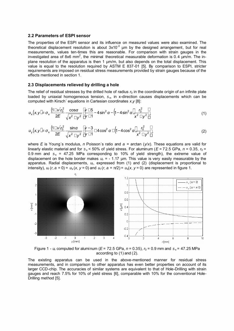
where E is Young´s modulus, ν Poisson´s ratio and α = arctan (y/x). These equations are valid for linearly elastic material and for σx < 50% of yield stress. For aluminum (E = 72.5 GPa, ν = 0.35, r0 = 0.9 mm and σx = 47.25 MPa corresponding to 10% of yield strength), the extreme value of displacement on the hole border makes ur = - 1.17 µm. This value is very easily measurable by the apparatus. Radial displacements, ur, expressed from (1) and (2) (displacement is proportional to intensity), ur (r, α = 0) = ux (x, y = 0) and ur (r, α = π/2) = ux(x, y = 0) are represented in figure 1.

Figure 1 - ur computed for aluminum (E = 72.5 GPa, ν = 0.35), r0 = 0.9 mm and σx = 47.25 MPa

according to (1) and (2).

The existing apparatus can be used in the above-mentioned manner for residual stress measurements, and in comparison to other apparatus has even better properties on account of its larger CCD-chip. The accuracies of similar systems are equivalent to that of Hole-Drilling with strain gauges and reach 7.5% for 10% of yield stress [6], comparable with 10% for the conventional Hole-Drilling method [5].

3 Stress � displacement relations Assuming a 2D-residual stress field at every depth under the surface, the relieved radial displacement, ur, at radius, r, on surface from center of a drilled hole of radius, r0, is

( ) ( ) ( ) ( ) ( ) ���hrB��hrAru 2cos,, minmaxESPIminmaxESPIr +⋅++⋅= , (3)

where σmax and σmin are the principal stresses acting at depth, h, α is the angle measured counterclockwise from σmax to the x-axis, AESPI and BESPI are calibration coefficients. Transforming displacements u0, u90 and u45 (displacement in counterclockwise angle directions of 0°, 90° and 45° to the x-axis) to p, q and t and normal stresses σx, σy and shear stress τxy to P, Q and T,

( ) 2/900 uup += , ( ) 2/900 uuq −= and ( ) 2/2 45900 uuut −+= , (4)

( ) 2/yx ��P += , ( ) 2/yx ��Q −= and xy�T = . (5)

Analogously to [9] we get the same expressions for the required principal stresses.

( )

++

⋅=ESPI

22

ESPIminmax 1

,b

tq�a

pE�� m and ( )qt� /arctan5.0= . (6)

Here β is the angle measured clockwise from the x-axis to the maximum principal stress direction, aESPI = 2 EAESPI/(1+ν) and bESPI = 2EBESPI are coefficients describing the relation between the measured displacements and stresses to be determined, which represents the main difference regarding [9].

A modified, two-dimensional, finite-element computation of the calibration coefficients for hole-drilling by the integral method [9] was used. A f ully automated model of step-wise varying stresses over the hole-depth was developed for determination of the calibration coefficient matrices (figure 2). For both matrices aESPI and bESPI two separate models are necessary (loading corresponding to biaxial stress and to pure shear, respectively). In the first model, axisymmetric, four-node, bilinear solid elements, in the second one axisymmetric four-node bilinear and Fourier quadrilateral, solid elements with nonlinear, asymmetric deformation, were used.

Maxwell�s reciprocity theorem states for any isotropic, linearly elastic structure that displacement at location �1� due to a unit force at �2� is equal to the displacement at �2� due to a unit force at �1� (i.e. the flexibility matrix is symmetric). This property was used to reduce significantly the number of computations that deliver matrices whose elements are cumulative sums of the required coefficients.

u1 u2 u3 u4 u5

F r0

rm

H,h

ESPI Sensor

Drilling unit

Spec

imen

Figure 2 � FEM � Model with load application

using Maxwell�s theorem. Figure 3 � Apparatus arrangement.

4 Experimental part

4.1 Apparatus The designed apparatus used (figure 3) consists of three main parts: ESPI-sensor, drilling unit and stiff frame to which different specimens can be attached. The CCD-chip resolution of the sensor camera is 768 x 576 pixels with a 256-bit color depth. The illumination angle of 28° and laser wavelength of 780 nm were the same for all experiments. Other sensor properties are described in section 2.2. For drilling, a standard pneumatic driven milling machine with mill diameter of 1.8 mm was used. Its rotation, radial and tangential feeds are controlled pneumatically by a separate computer which is connected by a trigger signal to the ESPI-computer. The measurement and determination of residual stresses is fully automatic.

4.2 Measurement and evaluation procedure The apparatus is able to measure displacements, ux and uy, perpendicular to the camera axis, z. For each direction four reference, phase-shifted speckle-images are recorded before drilling. After that a hole of incremental depth is drilled and another four speckle-images are recorded. By subtracting them from the reference images the relieved displacement fields, ux and uy, are determined. The second set of images is used as a reference for the following drilling step.

Within one step, the radial displacement field, ur, is computed from ux and uy. After that the direct and inverse Fourier transformations on circles are used to filter signal noise. According to (3) harmonics 0 and 2 are retained and from corresponding amplitudes the displacements u0, u90 and u45 are computed for different radii, rm, (figure 2). The rest of the values below the maximum radius are not utilized. The principal residual stresses and their direction are determined by (6). An example of original and filtered fields, ur, are shown in figures 4 and 5, where radial displacements are proportional to intensity (compare with figure 1).

Figure 4 � Radial displacements (unfiltered). Figure 5 � Radial displacements (filtered).

4.3 Specimens and results Specimens with constant stress over thickness

The simplest way to simulate one-dimensional tension was with a conventional tensile sample with holes drilled after loading. The behavior of aluminum Al7075 samples was investigated for various hole-depths and various stresses. These measurements were compared with strain gauge data and with the known stress state. The maximum difference between the ESPI measurement and the known stress was 4.5 % for stresses of 10 % of the material yield stress (compare with 7.5% in [6]).

Another specimen with a known residual stress distribution was a ring and plug with a diametrical interference, δ, (figure 6). The contact stress, p, between the ring and plug and the radial and tangential stresses as a function of radius, R, in the ring are given by the following equations:

( )2outin

2out

2in

2 RRRRE�

p−

= ;

−

−= 2

2out

2in

2out

2in

r 1R

RRR

pR� and

+

−= 2

2out

2in

2out

2in

t 1R

RRR

pR� . (3)

Figure 6 � Specimen with constant stress over

thickness. Figure 7 � Stress distribution in the plug and

ring.

During the assembly the plug was cooled down to �160°C by liquid nitrogen and the ring was heated to +40°C. The temperature difference of 200°C caused a radius difference, ∆Rin = 0.108 mm between both parts, which was sufficient for putting them together (minimal temperature difference corresponding to δ = 0.05 mm was 84°C). Various strain gauges were installed on the ring, by which the assembly symmetry and stress distribution was verified. The experimentally verified stress diagram is shown in figure 7 (material Al7075, E = 72.5 GPa, δ = 0.05 mm, Rin = 25 mm, Rout = 60 mm) together with ESPI-measurements (σtESPI, σrESPI). The maximum difference between them was 5.1 %.

Both specimen sides were used for measurements. The chosen thickness was a compromise between minimizing the influence of geometrical irregularities and the impact of drilling on one side or another.

Specimen with linearly changing stress over thickness Linearly changing stress was simulated on bent, 4.3 mm-thick, aluminum plates. These plates were fastened in a four-point-bending device (figure 8) and loaded by adjusting the screw at the base of the rig. This causes a plane strain state in the plate, which can be described analytically. Because of the lack of a direct force measurement and the non-linear dependence between loading angle and applied force, the load was determined by strain gauges attached directly to the upper part of the sample. The loading symmetry on the upper and lower surfaces was verified experimentally by strain gauges.

F F

F F

Load adjustment

Figure 8 � 4-point-bending device. Figure 9 � Measured stress distribution in upper part of bended plate.

The drilling was done in four 300 µm deep incremental steps up to the depth h = 1.2 mm, equal approximately to 1/4 of the plate thickness. An example of the stress distribution and data experimentally measured by ESPI for the above-mentioned aluminum, plate thickness t = 4.3 mm, width w = 45 mm and bending moment inducing strains εx = 610 µm/m and εy = - 80 µm/m on the specimen surface, is shown in figure 9. The maximum difference was 8.2 % for stress in the y-direction.

5 Conclusions According to the theoretical considerations about the applicability of this method based on basic computations and experiments, the existing apparatus can be used for residual stress measurements. It is possible to determine casual residual stresses with a relative error of 5 %. It represents a better result than the 10% for the conventional Hole-Drilling method which was used as a reference method by simple tension experiments.

Specimens with known internal stresses were designed and their stress distributions were measured by ESPI. The algorithm for automatic measurement and evaluation of residual stresses was designed. As a further step it is planned to provide measurements on real objects and compare them again with strain gauge results.

Acknowledgements The authors gratefully acknowledge the financial support of the grant of the Ministry for Industry and Trade of the Czech Republic No. MPO FT-TA/026-T10, the CTU grant 0710712 and the Christian Doppler Research Association (CDG).

References [1] DAINTY, J.C.: Laser speckle and related phenomena (Topics in Applied Physics 9), Springer-Verlag, Berlin

and New York, 1975.

[2] ARCHOBOLD, E., ENNOS, A.E.: Displacement measurement from double exposure laser photographs. Optica Acta, 19, 1972, 253�270.

[3] CLOUD, G. L.: Optical Methods of Engineering Analysis, Cambridge University Press, New York 1995.

[4] LU, J.: Handbook of Measurement of Residual Stresses, The Fairmont Press, Lilburn 1996.

[5] ASTM E 837-01: Standard test method for determining residual stresses by the hole-drilling strain gauge method, 2001.

[6] VIOTTI, M. R., KAUFMANN, G. H.: Accuracy and sensitivity of a hole drilling and digital speckle pattern interferometry combined techniquie to measure residual stresses, Optics and Lasers in Engineering, 41, 2004, 297�305.

[7] �EDIVÝ, O.: Grundlagen und Anwendung der ESPI für die Analyse elastisch-plastischer Werkstoffeigenschaften. Technische Universität Chemnitz, Chemnitz 2003.

[8] KAIBIRI, M.: Toward more accurate residual-stress measurement by the hole-drilling method: analysis of relieved-strain coefficients, Experimental Mechanics, 26, 1986, 14�24.

[9] SCHAJER, G.S.: Measurement of non-uniform residual stresses using the hole-drilling Method. Part II � Practical application of the integral method, Journal of Engineering Materials and Technology, 110, 1988, 344 � 349.