residual analysis for linear mixed modelsjmsinger/mae0610/mixedmodelresiduals.pdf · example of...
TRANSCRIPT

Residual analysis for linear mixed models
Julio M Singer
Departamento de EstatısticaUniversidade de Sao Paulo
in collaboration with
Juvencio Santos Nobre, UFC
JM Singer (USP) MAE0610 2011 1 / 1

Example of repeated measures
Study conducted at the School of Dentistry of the University of Sao
Paulo
Objective: compare the effect of an experimental toothbrush with
that of a conventional one with respect to bacterial plaque reduction
Design: bacterial plaque index measured on 32 pre-schoolers (16 with
conventional and 16 with experimental toothbrush) before and after
toothbrushing in 4 sessions spaced by 15 days
Repeated measures: same characteristic measured on each subject
more than once
Observations on each subject tend to be correlated
JM Singer (USP) MAE0610 2011 2 / 1

The data
Table 1: Bacterial plaque indices
1st session . . . 4th sessionBefore After . . . Before After
Subject Toothbrush brushing brushing . . . brushing brushing
1 conventional 1.05 1.00 . . . 1.13 0.942 conventional 1.07 0.62 . . . 1.15 0.853 experimental 0.82 0.62 . . . 1.78 1.39...
...... . . .
......
29 conventional 0.91 0.67 . . . 1.12 0.3730 experimental 1.06 0.70 . . . 1.12 1.0031 experimental 2.30 2.00 . . . 2.15 1.9032 conventional 1.15 1.00 . . . 1.26 1.00
JM Singer (USP) MAE0610 2011 3 / 1
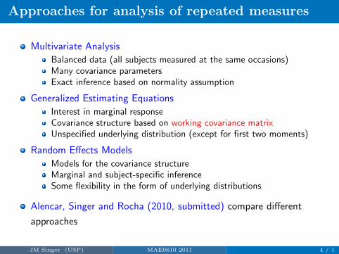
Approaches for analysis of repeated measures
Multivariate Analysis
Balanced data (all subjects measured at the same occasions)Many covariance parametersExact inference based on normality assumption
Generalized Estimating Equations
Interest in marginal responseCovariance structure based on working covariance matrixUnspecified underlying distribution (except for first two moments)
Random Effects Models
Models for the covariance structureMarginal and subject-specific inferenceSome flexibility in the form of underlying distributions
Alencar, Singer and Rocha (2010, submitted) compare different
approaches
JM Singer (USP) MAE0610 2011 4 / 1
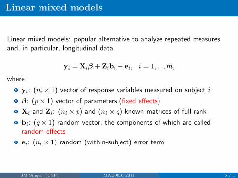
Linear mixed models
Linear mixed models: popular alternative to analyze repeated measuresand, in particular, longitudinal data.
yi = Xiβ + Zibi + ei, i = 1, ...,m,
where
yi: (ni × 1) vector of response variables measured on subject i
β: (p × 1) vector of parameters (fixed effects)
Xi and Zi: (ni × p) and (ni × q) known matrices of full rank
bi: (q × 1) random vector, the components of which are calledrandom effects
ei: (ni × 1) random (within-subject) error term
JM Singer (USP) MAE0610 2011 5 / 1
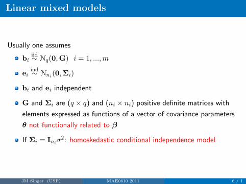
Linear mixed models
Usually one assumes
biiid∼ Nq(0,G) i = 1, ...,m
eiind∼ Nni
(0,Σi)
bi and ei independent
G and Σi are (q × q) and (ni × ni) positive definite matrices with
elements expressed as functions of a vector of covariance parameters
θ not functionally related to β
If Σi = Iniσ2: homoskedastic conditional independence model
JM Singer (USP) MAE0610 2011 6 / 1

BLUE and BLUP
Letting
y = (y⊤
1 , · · · ,y⊤
m)⊤, X = (X⊤
1 , · · · ,X⊤
m)⊤, Z = ⊕mi=1Zi
b = (b⊤
1 , · · · ,b⊤
m)⊤, e = (e⊤1 , · · · , e⊤
m)⊤
Γ = Im ⊗G, Σ = ⊕mi=1Σi
we can write the model more compactly as
y = Xβ + Zb+ e
Given Γ and Σ
Best Linear Unbiased Estimator (BLUE) of β : β = Ty
Best Linear Unbiased Predictor (BLUP) of b : b = ΓZ⊤Qy
with
T =(X⊤MX
)−1X⊤M
Q = M(I −XT)
M = V−1 = (ZΓZ⊤ +Σ)−1
JM Singer (USP) MAE0610 2011 7 / 1
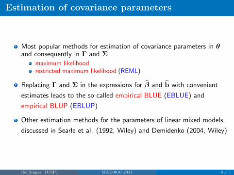
Estimation of covariance parameters
Most popular methods for estimation of covariance parameters in θand consequently in Γ and Σ
maximum likelihoodrestricted maximum likelihood (REML)
Replacing Γ and Σ in the expressions for β and b with convenient
estimates leads to the so called empirical BLUE (EBLUE) and
empirical BLUP (EBLUP)
Other estimation methods for the parameters of linear mixed models
discussed in Searle et al. (1992, Wiley) and Demidenko (2004, Wiley)
JM Singer (USP) MAE0610 2011 8 / 1
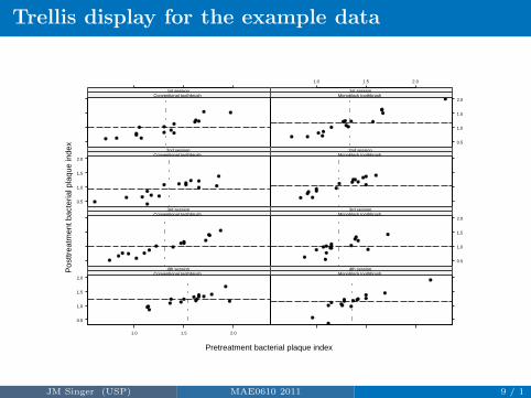
Trellis display for the example data
Conventional toothbrush1st session
0.5
1.0
1.5
2.0Monoblock toothbrush
1st session
1.0 1.5 2.0
0.5
1.0
1.5
2.0Conventional toothbrush
2nd sessionMonoblock toothbrush
2nd session
Conventional toothbrush3rd session
0.5
1.0
1.5
2.0Monoblock toothbrush
3rd session
0.5
1.0
1.5
2.0Conventional toothbrush
4th session
1.0 1.5 2.0
Monoblock toothbrush4th session
Pretreatment bacterial plaque index
Pos
ttrea
tmen
t bac
teria
l pla
que
inde
x
JM Singer (USP) MAE0610 2011 9 / 1
Linear mixed model for the example
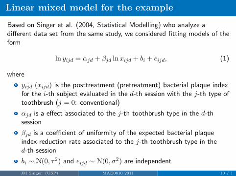
Based on Singer et al. (2004, Statistical Modelling) who analyze adifferent data set from the same study, we considered fitting models of theform
ln yijd = αjd + βjd lnxijd + bi + eijd, (1)
where
yijd (xijd) is the posttreatment (pretreatment) bacterial plaque indexfor the i-th subject evaluated in the d-th session with the j-th type oftoothbrush (j = 0: conventional)
αjd is a effect associated to the j-th toothbrush type in the d-thsession
βjd is a coefficient of uniformity of the expected bacterial plaqueindex reduction rate associated to the j-th toothbrush type in thed-th session
bi ∼ N(0, τ2) and eijd ∼ N(0, σ2) are independent
JM Singer (USP) MAE0610 2011 10 / 1
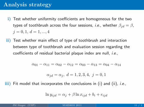
Analysis strategy
i) Test whether uniformity coefficients are homogeneous for the two
types of toothbrush across the four sessions, i.e., whether βjd = β,
j = 0, 1, d = 1, ..., 4
ii) Test whether main effect of type of toothbrush and interaction
between type of toothbrush and evaluation session regarding the
coefficients of residual bacterial plaque index are null, i.e.,
α01 − α11 = α02 − α12 = α03 − α13 = α04 − α14
αjd = αj , d = 1, 2, 3, 4, j = 0, 1
iii) Fit model that incorporates the conclusions in (i) and (ii), i.e.,
ln yijd = αj + β lnxijd + bi + eijd
JM Singer (USP) MAE0610 2011 11 / 1
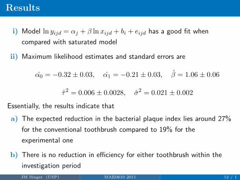
Results
i) Model ln yijd = αj + β lnxijd + bi + eijd has a good fit when
compared with saturated model
ii) Maximum likelihood estimates and standard errors are
α0 = −0.32 ± 0.03, α1 = −0.21± 0.03, β = 1.06 ± 0.06
τ2 = 0.006 ± 0.0028, σ2 = 0.021 ± 0.002
Essentially, the results indicate that
a) The expected reduction in the bacterial plaque index lies around 27%
for the conventional toothbrush compared to 19% for the
experimental one
b) There is no reduction in efficiency for either toothbrush within the
investigation period
JM Singer (USP) MAE0610 2011 12 / 1
Residual Analysis
Residuals frequently used to
evaluate validity of assumptions of statistical models
help in model selection
For standard (normal) linear models, residuals are used to verify
homoskedasticity
linearity of effects
presence of outliers
normality and independence of the errors
JM Singer (USP) MAE0610 2011 13 / 1

Type of residuals in linear mixed models
Cox and Snell (1968, JRSS-B): general definition of residuals for
models with single source of variability
Hilden-Minton (1995, PhD thesis UCLA), Verbeke and Lesaffre(1997, CSDA) or Pinheiro and Bates (2000, Springer): extension todefine three types of residuals that accommodate the extra source ofvariability present in linear mixed models, namely:
i) Marginal residuals, ξ = y −Xβ = M−1Qy, predictors of marginal
errors, ξ = y −E[y] = y −Xβ = Zb+ e
ii) Conditional residuals, e = y −Xβ − Zb = ΣQy, predictors of
conditional errors e = y −E[y|b] = y −Xβ − Zb
iii) BLUP, Zb, predictors of random effects, Zb = E[y|b]−E[y]JM Singer (USP) MAE0610 2011 14 / 1
Confounded Residuals
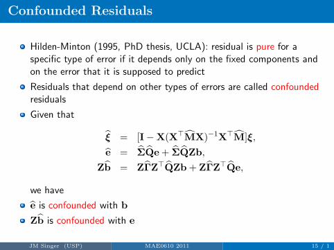
Hilden-Minton (1995, PhD thesis, UCLA): residual is pure for aspecific type of error if it depends only on the fixed components andon the error that it is supposed to predict
Residuals that depend on other types of errors are called confoundedresiduals
Given that
ξ = [I−X(X⊤MX)−1X⊤M]ξ,
e = ΣQe+ ΣQZb,
Zb = ZΓZ⊤QZb+ ZΓZ⊤Qe,
we have
e is confounded with b
Zb is confounded with e
JM Singer (USP) MAE0610 2011 15 / 1
Marginal Residuals
Since y = Xβ + ξ, plots of the marginal residuals (ξ) versus
explanatory variables may be employed to check linearity of y with
respect to such variables
Lesaffre and Verbeke (1998, Biometrics): Ri = V−1/2i ξi are residuals
to check appropriateness of the within-subjects covariance matrix
When ||Ini− RiR
⊤
i ||2 is small, within-subjects covariance matrix is
acceptable
JM Singer (USP) MAE0610 2011 16 / 1
Marginal Residuals: example
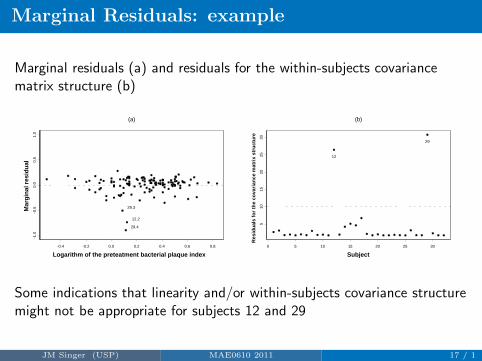
Marginal residuals (a) and residuals for the within-subjects covariancematrix structure (b)
-0.4 -0.2 0.0 0.2 0.4 0.6 0.8
Logarithm of the preteatment bacterial plaque index
-1.0
-0.5
0.0
0.5
1.0
Mar
gin
al r
esid
ual
(a)
12.2
29.3
29.4
0 5 10 15 20 25 30
Subject5
1015
2025
30
Res
idu
als
for
the
cova
rian
ce m
atri
x st
ruct
ure
(b)
12
29
Some indications that linearity and/or within-subjects covariance structuremight not be appropriate for subjects 12 and 29
JM Singer (USP) MAE0610 2011 17 / 1
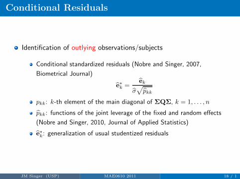
Conditional Residuals
Identification of outlying observations/subjects
Conditional standardized residuals (Nobre and Singer, 2007,
Biometrical Journal)
e∗k =ek
σ√pkk
pkk: k-th element of the main diagonal of ΣQΣ, k = 1, . . . , n
pkk: functions of the joint leverage of the fixed and random effects
(Nobre and Singer, 2010, Journal of Applied Statistics)
e∗k: generalization of usual studentized residuals
JM Singer (USP) MAE0610 2011 18 / 1
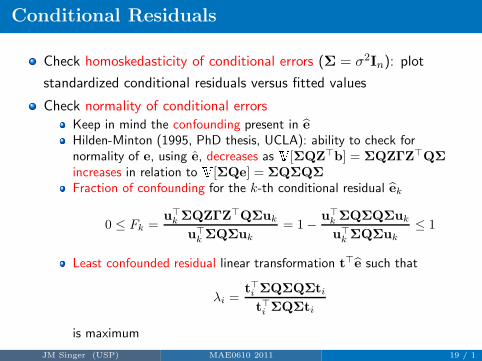
Conditional Residuals
Check homoskedasticity of conditional errors (Σ = σ2In): plot
standardized conditional residuals versus fitted values
Check normality of conditional errors
Keep in mind the confounding present in eHilden-Minton (1995, PhD thesis, UCLA): ability to check fornormality of e, using e, decreases as V[ΣQZ⊤b] = ΣQZΓZ⊤QΣincreases in relation to V[ΣQe] = ΣQΣQΣFraction of confounding for the k-th conditional residual ek
0 ≤ Fk =u⊤
kΣQZΓZ⊤QΣuk
u⊤
kΣQΣuk
= 1−u⊤
kΣQΣQΣuk
u⊤
kΣQΣuk
≤ 1
Least confounded residual linear transformation t⊤e such that
λi =t⊤iΣQΣQΣti
t⊤iΣQΣti
is maximum
JM Singer (USP) MAE0610 2011 19 / 1

Least Confounded Residuals: example
Least confounded residuals: homoskedastic and uncorrelated withvariance σ2
Check normality of the conditional errors via normal quantile plotswith simulated envelopes
Figure 3: Standardized conditional residuals (a) and simulated 95% confidenceenvelope for the standardized least confounded conditional residuals (b)
0 5 10 15 20 25 30
Subject
-4-2
02
4
Sta
nd
ard
ized
co
nd
itio
nal
res
idu
al
(a)
12.2 29.4
-2 -1 0 1 2
Quantiles of N(0,1)
-4-2
02
4
Lea
st c
on
fou
nd
ed r
esid
ual
(b)
JM Singer (USP) MAE0610 2011 20 / 1

EBLUP
EBLUP: reflects the difference between the predicted responses for
the i-th subject and the population average
Useful to detect outlying subjects: plot ζi = b⊤
i {V[bi − bi]}−1bi
versus subject indices
Useful to assess which subjects are sensitive to homogeneity of thecovariance matrices of the random effects
Pinheiro and Bates (2000, Springer): scatter plot matrix of thepredicted random effectsNobre (2004, MSc dissertation, USP): perturbation of the covariancematrix of the i-th random effect by letting V[bi] = wiG andidentifying subjects which are sensitive to this perturbation via localinfluence methods
JM Singer (USP) MAE0610 2011 21 / 1
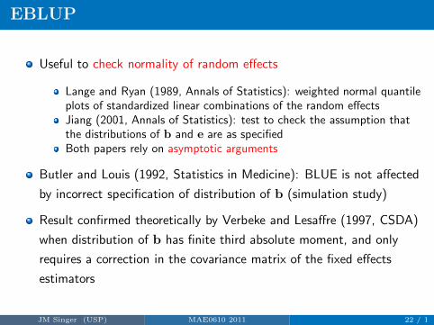
EBLUP
Useful to check normality of random effects
Lange and Ryan (1989, Annals of Statistics): weighted normal quantileplots of standardized linear combinations of the random effectsJiang (2001, Annals of Statistics): test to check the assumption thatthe distributions of b and e are as specifiedBoth papers rely on asymptotic arguments
Butler and Louis (1992, Statistics in Medicine): BLUE is not affected
by incorrect specification of distribution of b (simulation study)
Result confirmed theoretically by Verbeke and Lesaffre (1997, CSDA)
when distribution of b has finite third absolute moment, and only
requires a correction in the covariance matrix of the fixed effects
estimators
JM Singer (USP) MAE0610 2011 22 / 1

EBLUP: example
Figure 4: EBLUP (a) and Cook’s |dmax| for the perturbed variance ofrandom effects (b)
0 5 10 15 20 25 30
Subject
-0.3
-0.2
-0.1
0.0
0.1
0.2
0.3
EB
LU
P
(a)
29
0 5 10 15 20 25 30
Subject
0.0
0.2
0.4
0.6
0.8
1.0
|dm
ax|
(b)
29
JM Singer (USP) MAE0610 2011 23 / 1
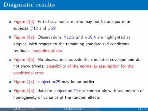
Diagnostic results
Figure 2(b): Fitted covariance matrix may not be adequate for
subjects #12 and #29
Figure 3(a): Observations #12.2 and #29.4 are highlighted as
atypical with respect to the remaining standardized conditional
residuals: possible outliers
Figure 3(b): No observations outside the simulated envelope and do
not show trends: plausibility of the normality assumption for the
conditional error
Figure 4(a): subject #29 may be an outlier
Figure 4(b): data for subject # 29 not compatible with assumption of
homogeneity of variance of the random effects
JM Singer (USP) MAE0610 2011 24 / 1
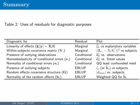
Summary
Table 2: Uses of residuals for diagnostic purposes
Diagnostic for Residual Plot
Linearity of effects (E[y] = Xβ) Marginal ξk vs explanatory variablesWithin-subjects covariance matrix (Vi) Marginal ||Ini
− RiR⊤
i ||2 vs subjects
Presence of outlying observations Conditional e∗
k vs. observationsHomoskedasticity of conditional errors (ei) Conditional e∗
k vs. fitted valuesNormality of conditional errors (ei) Conditional QQ least confounded resid
Presence of outlying subjects EBLUP ζi (or bi) vs subjectsRandom effects covariance structure (G) EBLUP |dmax| vs. subjects
Normality of the random effects (bi) EBLUP Weighted QQ for bi
JM Singer (USP) MAE0610 2011 25 / 1
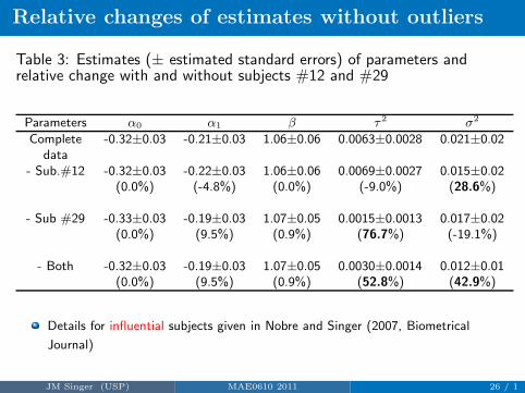
Relative changes of estimates without outliers
Table 3: Estimates (± estimated standard errors) of parameters andrelative change with and without subjects #12 and #29
Parameters α0 α1 β τ 2 σ2
Complete -0.32±0.03 -0.21±0.03 1.06±0.06 0.0063±0.0028 0.021±0.02data
- Sub.#12 -0.32±0.03 -0.22±0.03 1.06±0.06 0.0069±0.0027 0.015±0.02(0.0%) (-4.8%) (0.0%) (-9.0%) (28.6%)
- Sub #29 -0.33±0.03 -0.19±0.03 1.07±0.05 0.0015±0.0013 0.017±0.02(0.0%) (9.5%) (0.9%) (76.7%) (-19.1%)
- Both -0.32±0.03 -0.19±0.03 1.07±0.05 0.0030±0.0014 0.012±0.01(0.0%) (9.5%) (0.9%) (52.8%) (42.9%)
Details for influential subjects given in Nobre and Singer (2007, Biometrical
Journal)
JM Singer (USP) MAE0610 2011 26 / 1
Discussion
Incorrect identification of influential subjects may occur when the
covariance structure is misspecified (Fei and Pan, 2003, 18-th
International Workshop on Statistical Modelling)
Wolfinger (1993, Communications in Statistics), Rutter and Elashoff
(1994, Statistics in Medicine), Grady and Helms (1995, Statistics in
Medicine) or Rocha and Singer (2010, in preparation ): methods of
selection of the covariance structure in mixed models
JM Singer (USP) MAE0610 2011 27 / 1
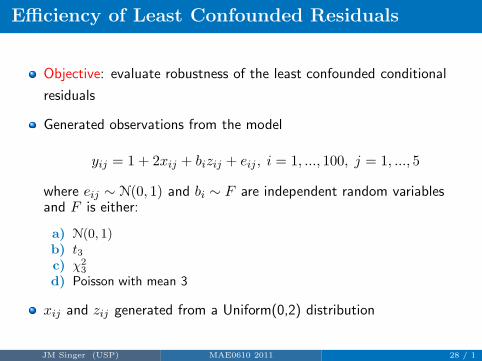
Efficiency of Least Confounded Residuals
Objective: evaluate robustness of the least confounded conditional
residuals
Generated observations from the model
yij = 1 + 2xij + bizij + eij , i = 1, ..., 100, j = 1, ..., 5
where eij ∼ N(0, 1) and bi ∼ F are independent random variablesand F is either:
a) N(0, 1)b) t3c) χ2
3
d) Poisson with mean 3
xij and zij generated from a Uniform(0,2) distribution
JM Singer (USP) MAE0610 2011 28 / 1
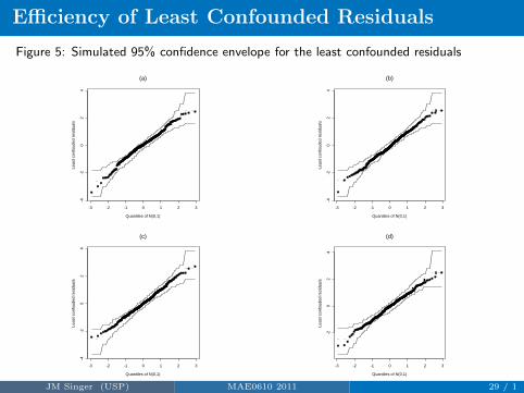
Efficiency of Least Confounded Residuals
Figure 5: Simulated 95% confidence envelope for the least confounded residuals
Quantiles of N(0,1)
Leas
t con
foud
ed r
esid
uals
-3 -2 -1 0 1 2 3
-4-2
02
4(a)
Quantiles of N(0,1)
Leas
t con
foud
ed r
esid
uals
-3 -2 -1 0 1 2 3
-4-2
02
4
(b)
Quantiles of N(0,1)
Leas
t con
foud
ed r
esid
uals
-3 -2 -1 0 1 2 3
-4-2
02
4
(c)
Quantiles of N(0,1)
Leas
t con
foud
ed r
esid
uals
-3 -2 -1 0 1 2 3
-20
24
(d)
JM Singer (USP) MAE0610 2011 29 / 1
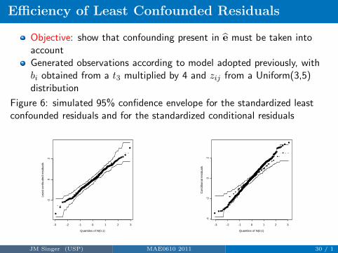
Efficiency of Least Confounded Residuals
Objective: show that confounding present in e must be taken intoaccountGenerated observations according to model adopted previously, withbi obtained from a t3 multiplied by 4 and zij from a Uniform(3,5)distribution
Figure 6: simulated 95% confidence envelope for the standardized leastconfounded residuals and for the standardized conditional residuals
Quantiles of N(0,1)
Leas
t con
foud
ed r
esid
uals
-3 -2 -1 0 1 2 3
-20
2
Quantiles of N(0,1)
Con
ditio
nal r
esid
uals
-3 -2 -1 0 1 2 3
-4-2
02
JM Singer (USP) MAE0610 2011 30 / 1
Conclusions and computational aspects
Standardized least confounded residuals may be employed to evaluate
the plausibility of the normality assumption for the conditional error
even when the random effects are not normal
Some diagnostic tools implemented in S-plus (NLME) and R (NLME
and lme4) packages
Modifications needed to take confounding and correct standardization
of the conditional residuals in consideration
Codes employed for the analysis of the example and the simulation
developed in R (function lmmresdidual ) and can be obtained directly
from the authors
JM Singer (USP) MAE0610 2011 31 / 1

References
Butler, S.M. and Louis, T.A. (1992). Random effects models withnon-parametric priors. Statistics in Medicine 11, 1981–2000.
Cox, D.R. and Snell, E.J. (1968) A general definition of residuals (withdiscussion). Journal Royal Statistical Society B 30, 248–275.
Demidenko, E. (2004). Mixed models: theory and applications. New York:John Wiley & Sons.
Fei, Y. & Pan, J. (2003). Influence assessments for longitudinal data inlinear mixed models. In 18-th International Workshop on Statistical
Modelling. Eds. G. Verbeke, G. Molenberghs, M. Aerts and S. Fieuws.Leuven: Belgium, 143–148.
Grady, J.J. and Helms, R.W. (1995).Model selection techniques for thecovariance matrix for incomplete longitudinal data. Statistics in Medicine
14, 1397–1416.
Hilden-Minton, J.A. (1995). Multilevel diagnostics for mixed and
hierarchical linear models. PhD Thesis, UCLA, Los Angeles.
Jiang, J. (2001). Goodness-of-fit tests for mixed model diagnostics. TheAnnals of Statistics 29, 1137–1164.
JM Singer (USP) MAE0610 2011 32 / 1
References
Lange, N. and Ryan, L. (1989). Assessing normality in random effectsmodels. The Annals of Statistics 17, 624–642.
Lesaffre, E. and Verbeke, G. (1998). Local influence in linear mixed models.Biometrics 54, 570–582.
Nobre, J.S. (2004). Metodos de diagnostico para modelos lineares mistos.
Sao Paulo: Instituto de Matematica e Estatıstica, Universidade de SaoPaulo. M.Sc. dissertation (in Portuguese).
Nobre, J.S. and Singer, J.M. (2007). Residual analysis for linear mixedmodels. Biometrical Journal, 49, 863–875.
Nobre, J.S. and Singer, J.M. (2011). Leverage analysis for linear mixedmodels. Journal of Applied Statistics, 38, 1063–1072.
Pinheiro, J.C. and Bates, D.M. (2000). Mixed-effects in S and S-PLUS.Springer, New York.
Searle, S.R., Casella, G. and McCullogh, C.E. (1992). Variance components.New York: Jonh Wiley & Sons.
JM Singer (USP) MAE0610 2011 33 / 1
References
Singer, J.M., Nobre, J.S. and Sef, H.C. (2004). Regression models forpretest/posttest data in blocks. Statistical Modelling 4, 324–338.
Rocha, F.M.M. and Singer, J.M. (2009). Selection of fixed and randomeffects in linear mixed models. Submitted
Rutter, C.M. and Elashoff, R.M. (1994). Analysis of longitudinal data:random coefficient regression modelling. Statistics in Medicine 13,1211–1231.
Verbeke, G. and Lesaffre, E. (1996b). Large samples properties of themaximum likelihood estimators in linear mixed models with misspecifiedrandom-effects distributions. Technical report, Biostatistical Centre forClinical Trials, Catholic University of Leuven, Belgium.
Verbeke, G. and Lesaffre, E. (1997). The effect of misspecifying therandom-effects distributions in linear mixed models for longitudinal data.Computational Statistics & Data Analysis 23, 541–556.
Wolfinger, R. (1993). Covariance structure selection in general mixedmodels. Communications in Statistics-Simulation 22, 1079–1106.
JM Singer (USP) MAE0610 2011 34 / 1