ORIGINAL PAPER - EXPLORATION GEOPHYSICS

Reservoir properties prediction using extended elastic impedance:the case of Nianga field of West African Congo basin

Charles Prisca Samba1 • Hongmei Lu2 • Habib Mukhtar2

Received: 15 September 2016 / Accepted: 21 January 2017 / Published online: 1 March 2017

� The Author(s) 2017. This article is published with open access at Springerlink.com

Abstract Simultaneous seismic inversion and extended

elastic impedance (EEI) were applied to obtain quantitative

estimates of porosity, water saturation, and shale volume

over Nianga field of Congo basin, West Africa. The opti-

mum angle at which EEI log and the target petrophysical

parameter give the maximum correlation was meticulously

analyzed by additionally incorporating the concept of rel-

ative rock physics. Prestack seismic data were simultane-

ously inverted into Vp, acoustic, and gradient impedances.

The last two broadband inverted volumes were projected to

Chi angles corresponding to the target petrophysical

parameters, and three broadband EEI volumes were

obtained. At well control points, the linear trends based on

specific lithology between EEI and petrophysical parame-

ters were then used to transform EEI volumes into quan-

titative porosity, water saturation, and shale volume cubes.

In order to obtain the reservoir facies distribution, another

concept of minimum energy angle was used to generate the

background EEI cube, thereby enabling the mapping of

reservoir facies. From quantitative porosity, water satura-

tion, shale content, and background EEI cubes, favorable

zones have been pinpointed which may suggest possible

drilling locations for future development of the field.

Keywords Extended elastic impedance � Simultaneous

inversion � Relative rock physics

Introduction

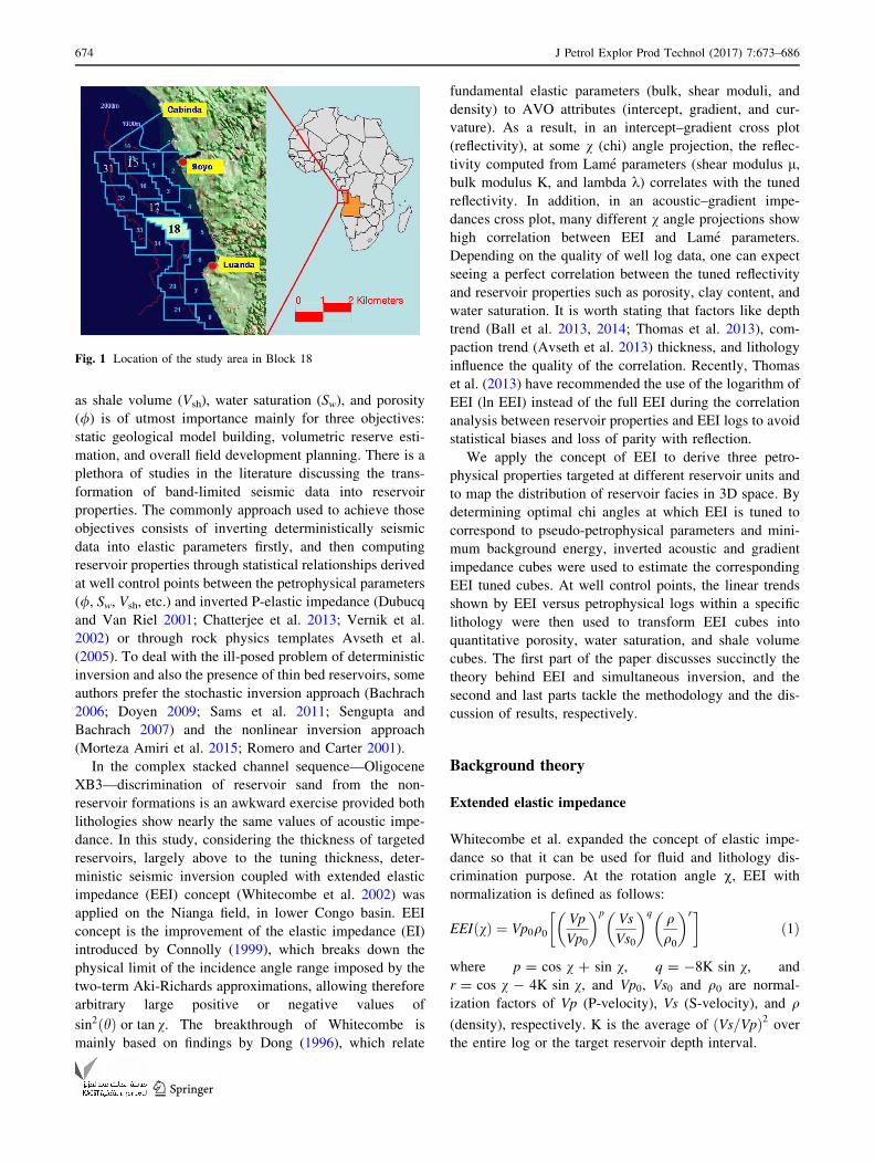
Block 18 is situated in the southernmost portion of the

lower Congo basin (Fig. 1)a Tertiary depocentre along the

West African passive continental margin and is a product

of Late Jurassic to Early Cretaceous rifting which heralded

the first stage in the eventual opening of the southern

Atlantic. Syn-rift sediments in the Lower Cretaceous

(Neocomian–Barremian) are represented by the coarse

siliciclastics, and the organic-rich lacustrine source

deposits of the Bucomazi Formation, which lie uncon-

formably on top of Pre-Cambrian fault blocks.

The Nianga field is located in deep water in the north

central region of Block 18, approximately 175 km offshore

to the northwest of Luanda, and is separated from the

neighboring Mamba field to the immediate west by a

structural saddle and a stratigraphic pinch out. It is the

largest field within the block development area, with esti-

mated recoverable reserves greater than 250 MMBO. It is a

four-way dipping low-relief turtle structure, some 11 km

long and up to 5 km wide. There are two Oligocene

reservoir levels: aerially extensive but thin sheet sand—the

Oligocene XB2, and a more complex stacked channel

sequence—the Oligocene XB3; the XB3 is the most

important in terms of recoverable reserves. The field was

discovered in 1999, and an appraisal phase in 2001

involved the drilling of two exploration wells which con-

firmed a common OWC between the XB2 and the XB3

sands and the existence of a gas cap. A subsequent inter-

ference test proved that there was effective connectivity in

the sands between the separate locations.

A robust inversion of petrophysical parameters and the

distribution of the reservoir facies in 3D space are con-

sidered as key objectives for Nianga field development.

The inversion of important petrophysical parameters such

& Charles Prisca Samba

sambadebima@hotmail.com

1 Petroleum Exploration and Production Research Institute of

Sinopec, Beijing, China

2 Faculty of Earth Resources, Key Laboratory of Tectonics and

Petroleum Resources, China University of Geosciences,

Wuhan 430074, Hubei, China

123

J Petrol Explor Prod Technol (2017) 7:673–686

DOI 10.1007/s13202-017-0328-0

as shale volume (Vsh), water saturation (Sw), and porosity

(/) is of utmost importance mainly for three objectives:

static geological model building, volumetric reserve esti-

mation, and overall field development planning. There is a

plethora of studies in the literature discussing the trans-

formation of band-limited seismic data into reservoir

properties. The commonly approach used to achieve those

objectives consists of inverting deterministically seismic

data into elastic parameters firstly, and then computing

reservoir properties through statistical relationships derived

at well control points between the petrophysical parameters

(/, Sw, Vsh, etc.) and inverted P-elastic impedance (Dubucq

and Van Riel 2001; Chatterjee et al. 2013; Vernik et al.

2002) or through rock physics templates Avseth et al.

(2005). To deal with the ill-posed problem of deterministic

inversion and also the presence of thin bed reservoirs, some

authors prefer the stochastic inversion approach (Bachrach

2006; Doyen 2009; Sams et al. 2011; Sengupta and

Bachrach 2007) and the nonlinear inversion approach

(Morteza Amiri et al. 2015; Romero and Carter 2001).

In the complex stacked channel sequence—Oligocene

XB3—discrimination of reservoir sand from the non-

reservoir formations is an awkward exercise provided both

lithologies show nearly the same values of acoustic impe-

dance. In this study, considering the thickness of targeted

reservoirs, largely above to the tuning thickness, deter-

ministic seismic inversion coupled with extended elastic

impedance (EEI) concept (Whitecombe et al. 2002) was

applied on the Nianga field, in lower Congo basin. EEI

concept is the improvement of the elastic impedance (EI)

introduced by Connolly (1999), which breaks down the

physical limit of the incidence angle range imposed by the

two-term Aki-Richards approximations, allowing therefore

arbitrary large positive or negative values of

sin2ðhÞ or tan v. The breakthrough of Whitecombe is

mainly based on findings by Dong (1996), which relate

fundamental elastic parameters (bulk, shear moduli, and

density) to AVO attributes (intercept, gradient, and cur-

vature). As a result, in an intercept–gradient cross plot

(reflectivity), at some v (chi) angle projection, the reflec-

tivity computed from Lame parameters (shear modulus l,bulk modulus K, and lambda k) correlates with the tuned

reflectivity. In addition, in an acoustic–gradient impe-

dances cross plot, many different v angle projections show

high correlation between EEI and Lame parameters.

Depending on the quality of well log data, one can expect

seeing a perfect correlation between the tuned reflectivity

and reservoir properties such as porosity, clay content, and

water saturation. It is worth stating that factors like depth

trend (Ball et al. 2013, 2014; Thomas et al. 2013), com-

paction trend (Avseth et al. 2013) thickness, and lithology

influence the quality of the correlation. Recently, Thomas

et al. (2013) have recommended the use of the logarithm of

EEI (ln EEI) instead of the full EEI during the correlation

analysis between reservoir properties and EEI logs to avoid

statistical biases and loss of parity with reflection.

We apply the concept of EEI to derive three petro-

physical properties targeted at different reservoir units and

to map the distribution of reservoir facies in 3D space. By

determining optimal chi angles at which EEI is tuned to

correspond to pseudo-petrophysical parameters and mini-

mum background energy, inverted acoustic and gradient

impedance cubes were used to estimate the corresponding

EEI tuned cubes. At well control points, the linear trends

shown by EEI versus petrophysical logs within a specific

lithology were then used to transform EEI cubes into

quantitative porosity, water saturation, and shale volume

cubes. The first part of the paper discusses succinctly the

theory behind EEI and simultaneous inversion, and the

second and last parts tackle the methodology and the dis-

cussion of results, respectively.

Background theory

Extended elastic impedance

Whitecombe et al. expanded the concept of elastic impe-

dance so that it can be used for fluid and lithology dis-

crimination purpose. At the rotation angle v, EEI with

normalization is defined as follows:

EEI vð Þ ¼ Vp0q0Vp

Vp0

� �pVs

Vs0

� �q qq0

� �r� �ð1Þ

where p = cos v ? sin v, q = -8K sin v, and

r = cos v - 4K sin v, and Vp0, Vs0 and q0 are normal-

ization factors of Vp (P-velocity), Vs (S-velocity), and q

(density), respectively. K is the average of ðVs=VpÞ2 over

the entire log or the target reservoir depth interval.

Fig. 1 Location of the study area in Block 18

674 J Petrol Explor Prod Technol (2017) 7:673–686

123

Obtaining EEI reflectivity volumes at v = 0� and

v = 90� so that they can be transformed into acoustic and

gradient impedances, respectively, was one of the reasons

leading to the development of the EEI approach. Therefore,

Eq. (1) can also be written as follows:

EEI vð Þ ¼ AI0AI

AI0

� �cosvGI

AI0

� �sinvð2Þ

where AI0 is the normalization factor of AI (P-impedance)

and GI is the gradient impedance.

Equation (2) can also be expressed in logarithm scale as

lnEEI vð Þ ¼ lnAI0 þ cos vlnAI

AI0

� �þ sin vln

GI

AI0

� �ð3Þ

v is considered as the rotational angle in the intercept–

gradient (AB) plane or ln GI–ln AI cross plot. It is related

to the angle of incidence h as follows:

tan v ¼ sin2 h ð4Þ

Equation (4) extends the range of measured data

imposed by sin2h (0\ sin2 h B 1) to minus and plus

infinities. By substituting Eq. (4) into the two-term

Zoeppritz linearization equation, one obtains

Rv ¼ Aþ B tan v ð5Þ

A and B are, respectively, the reflectivities of the

intercept and gradient. If we assume at v = v0, R(v0) = 0,

one gets,

tan v0 ¼ �A

Bð6Þ

The minimum energy angle (v0) (Hicks and Francis

2006) is the angle at which reflectivity of the two-term

AVO approximation is zero. The equivalent h angle of v0is commonly beyond the range of recorded seismic, but

if it happens to be within the recorded angle of seismic

gather, one might expect to see a phase reversal of

seismic reflection. Since the impedance contrast at the

shale–shale interface is usually negligible at minimum

energy, synthetic seismic obtained for this angle is

referred to as background trend. This will definitely help

to identify bodies highly contrasting within the

background volume.

Simultaneous inversion

By convolving the AVO approximation equation of Wig-

gins et al. (1983) with wavelet W (h), the synthetic seismic

trace is written as follows:

SPP hð Þ ¼ a=2W hð ÞDln AIð Þ þ b=2W hð ÞDdln GIð Þþ c=2W hð ÞDdln Vp

� �ð7Þ

where a ¼ 1þ aGIbþ aVpc, b ¼ sin2 h, c ¼ sin2 h tan2 h.

aGI is the gradient coefficient of the linear equation GI

(in y-axis) versus AI (in x-axis)

aVpis the gradient coefficient of the linear equation Vp

(in y-axis) versus AI (in x-axis)

dln Vp

� �is the deviation away from the linear equation

Vp (in y-axis) versus AI (in x-axis)

dln GIð Þ is the deviation away from the linear equation

GI (in y-axis) versus AI (in x-axis)

In the matrix form, Eq. (7) is written as follows:

Spp h1ð ÞSpp h2ð Þ

..

.

Spp hNð Þ

266664

377775

¼

a h1ð Þ2

W h1ð ÞD b h1ð Þ2

W h1ð ÞD c h1ð Þ2

W h1ð ÞD

a h2ð Þ2

W h2ð ÞD b h2ð Þ2

W h2ð ÞD c h2ð Þ2

W h2ð ÞD

..

. ... ..

.

a hNð Þ2

W hNð ÞD b hNð Þ2

W hNð ÞD c hNð Þ2

W hNð ÞD

266666666664

377777777775

ln AIð Þd ln GIð Þd lnðVpÞ

264

375

ð8Þ

The diagonal matrix D is composed of the difference

operation D as in (Hampson et al. 2005) and applied to

each ln(AI), dln VPð Þ and dln GIð Þ.The last column vector composed of ln(AI), dln VPð Þ and

dln GIð Þ is also represented by ln(Z). W h1::Nð Þ is a banded

matrix composed of extracted wavelets per partial angle

stack. SPP h1::Nð Þ is a column vector of the near-, mid-, and

far-seismic traces.

To solve Eq. (8) for ln Zð Þ, i.e., ln(AI), dln VPð Þ and

dln GIð Þ, the following total objective function is minimized:

Sreal � X � ln Zð Þ2þlln Zð Þ � ln Z0ð Þ2 ð9Þ

where l is the model weight, it has to be small to guarantee

the inversion driven by real seismic data.

Z0 is the initial model with which the inversion starts.

The conjugate gradient method is used to iteratively

modify ln(Z) until the difference between the synthetic

seismic data Spp(h) and real seismic data Sreal(h) is mini-

mized for near-, mid-, and far-stack angles. It is then

straightforward to derive Z by exponentiation of ln(Z).

Methodology

The proposed methodology aims at estimating tuned EEI

cubes which approximately correspond to minimum

background energy and petrophysical parameters such as

porosity, water saturation, and shale volume cubes.

J Petrol Explor Prod Technol (2017) 7:673–686 675

123

Figure 2 shows the workflow of the methodology used

in this study. It starts from (1) well log quality control

(QC) and conditioning to ensure that the required data

are available and physically reasonable in support of

petrophysics and rock physics activities; (2) computation

of EEI logs for different v angles using Eq. (1) or Eq. (2)

and the determination of the optimum angle that gives

the best correlation (positive or negative) between EEI

with the petrophysical target logs (porosity, shale vol-

ume, and water saturation); (3) QC, conditioning and

simultaneous inversion of prestack time-migrated partial

angle stacks such as near (5�–18�), mid (18�–31�), andfar (31�–45�) into P-wave velocity, acoustic, and gradi-

ent impedances; (4) computation of equivalent EEI

volume through Eq. (3) by using optimal angles; and (5)

transformation of EEI volumes into quantitative petro-

physical properties.

Reservoir facies distribution can be captured through

the concept of minimum energy angle (Eq. 6).The easi-

est approach to determine this angle is to compute the

EEI log spectrum with v ranging from -90� to ?90�(with an increment angle of 1).The determination of

minimum energy angle v0 is a visual process by ana-

lyzing the entire log spectrum in order to pinpoint zones

where anomalies are better characterized. Once the angle

v0 is determined, step 4 is then applied to generate

equivalent EEI volume.

Result and discussion

Data gathering and quality check

This step ensures that the required data are available in

support of petrophysics and rock physics activities; it deals

with improving well data which involve gaps correction

and other unavoidable problems with gathered data. It also

accounts for up-scaling when the need arises. The stage is

an intensely visual process, requiring visualization tools

and interactive manipulation widgets to make the process

smooth, easy, and accurate.

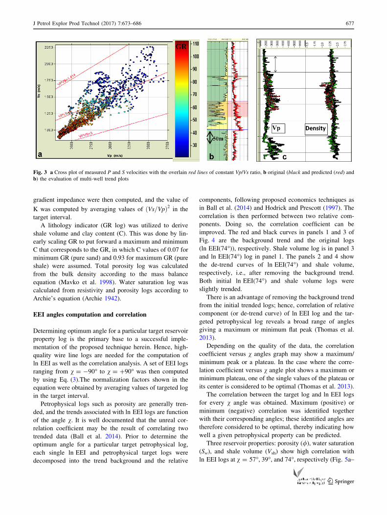
All succeeding steps in the workflow depend on the

quality and veracity of this step in the process. In this

research, the measured Vp and Vs logs were of good

quality, as shown in Fig. 3. In Fig. 3a, the red lines rep-

resenting constant Vp/Vs ratio showed that the values of

both Vp and Vs are in a physically reasonable range. In

addition, Vs log was also assessed by comparing measured

versus predicted logs, as shown in Fig. 3b, where the black

curve represents the measured (original) log and the red

curve is the Greenberg–Castagna predicted log. The eval-

uation of multi-well depth trend plots (Fig. 3b) revealed

that there were no spurious values for the velocity and

density logs, as no circles points (each well is represented

by different colors) deviated far away from the general

trend. Elastic parameters such as acoustic impedance and

Well Logs Data

Gathering, QC, Conditioning

Near Mid Far

Determination of minimum energy angle

Optimal chi angle

Vp Vs Vsh Sw

Correlation

Simultaneous Inversion

AI, GI

Computation of EEI logs or EEI spectrum

Data Conditioning

Seismic data (Pre-stack time migrated)

Computation of Backgroung minimum energy Computation of lnEEI/EEI

, Vsh and Sw

Quantitative , Vsh and Sw cubes

Fig. 2 Detailed workflow of

the methodology

676 J Petrol Explor Prod Technol (2017) 7:673–686

123

gradient impedance were then computed, and the value of

K was computed by averaging values of ðVs=VpÞ2 in the

target interval.

A lithology indicator (GR log) was utilized to derive

shale volume and clay content (C). This was done by lin-

early scaling GR to put forward a maximum and minimum

C that corresponds to the GR, in which C values of 0.07 for

minimum GR (pure sand) and 0.93 for maximum GR (pure

shale) were assumed. Total porosity log was calculated

from the bulk density according to the mass balance

equation (Mavko et al. 1998). Water saturation log was

calculated from resistivity and porosity logs according to

Archie’s equation (Archie 1942).

EEI angles computation and correlation

Determining optimum angle for a particular target reservoir

property log is the primary base to a successful imple-

mentation of the proposed technique herein. Hence, high-

quality wire line logs are needed for the computation of

ln EEI as well as the correlation analysis. A set of EEI logs

ranging from v = -90� to v = ?90� was then computed

by using Eq. (3).The normalization factors shown in the

equation were obtained by averaging values of targeted log

in the target interval.

Petrophysical logs such as porosity are generally tren-

ded, and the trends associated with ln EEI logs are function

of the angle v. It is well documented that the unreal cor-

relation coefficient may be the result of correlating two

trended data (Ball et al. 2014). Prior to determine the

optimum angle for a particular target petrophysical log,

each single ln EEI and petrophysical target logs were

decomposed into the trend background and the relative

components, following proposed economics techniques as

in Ball et al. (2014) and Hodrick and Prescott (1997). The

correlation is then performed between two relative com-

ponents. Doing so, the correlation coefficient can be

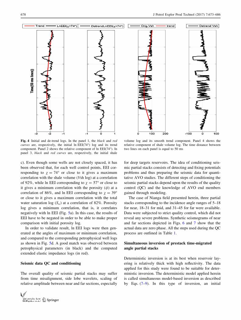
improved. The red and black curves in panels 1 and 3 of

Fig. 4 are the background trend and the original logs

(ln EEI(74�)), respectively. Shale volume log is in panel 3

and ln EEI(74�) log in panel 1. The panels 2 and 4 show

the de-trend curves of ln EEI(74�) and shale volume,

respectively, i.e., after removing the background trend.

Both initial ln EEI(74�) and shale volume logs were

slightly trended.

There is an advantage of removing the background trend

from the initial trended logs; hence, correlation of relative

component (or de-trend curve) of ln EEI log and the tar-

geted petrophysical log reveals a broad range of angles

giving a maximum or minimum flat peak (Thomas et al.

2013).

Depending on the quality of the data, the correlation

coefficient versus v angles graph may show a maximum/

minimum peak or a plateau. In the case where the corre-

lation coefficient versus v angle plot shows a maximum or

minimum plateau, one of the single values of the plateau or

its center is considered to be optimal (Thomas et al. 2013).

The correlation between the target log and ln EEI logs

for every v angle was obtained. Maximum (positive) or

minimum (negative) correlation was identified together

with their corresponding angles; these identified angles are

therefore considered to be optimal, thereby indicating how

well a given petrophysical property can be predicted.

Three reservoir properties: porosity (/), water saturation(Sw), and shale volume (Vsh) show high correlation with

ln EEI logs at v = 57�, 39�, and 74�, respectively (Fig. 5a–

Fig. 3 a Cross plot of measured P and S velocities with the overlain red lines of constant Vp/Vs ratio, b original (black and predicted (red) and

b) the evaluation of multi-well trend plots

J Petrol Explor Prod Technol (2017) 7:673–686 677

123

c). Even though some wells are not closely spaced, it has

been observed that, for each well control points, EEI cor-

responding to v = 74� or close to it gives a maximum

correlation with the shale volume (Vsh log) at a correlation

of 92%, while ln EEI corresponding to v = 57� or close toit gives a minimum correlation with the porosity (/) at acorrelation of 86%, and ln EEI corresponding to v = 39�or close to it gives a maximum correlation with the total

water saturation log (Sw) at a correlation of 82%. Porosity

log gives a minimum correlation, that is, it correlates

negatively with ln EEI (Fig. 5a). In this case, the results of

EEI have to be negated in order to be able to make proper

comparison with initial porosity log.

In order to validate result, ln EEI logs were then gen-

erated at the angles of maximum or minimum correlation,

and compared to the corresponding petrophysical well logs

as shown in Fig. 5d. A good match was observed between

petrophysical parameters (in black) and the computed

extended elastic impedance logs (in red).

Seismic data QC and conditioning

The overall quality of seismic partial stacks may suffer

from time misalignment, side lobe wavelets, scaling of

relative amplitude between near and far sections, especially

for deep targets reservoirs. The idea of conditioning seis-

mic partial stacks consists of detecting and fixing potentials

problems and thus preparing the seismic data for quanti-

tative AVO studies. The different steps of conditioning the

seismic partial stacks depend upon the results of the quality

control (QC) and the knowledge of AVO end members

gained through modeling.

The case of Nianga field presented herein, three partial

stacks corresponding to the incidence angle ranges of 5–18

for near, 18–31 for mid, and 31–45 for far were available.

Data were subjected to strict quality control, which did not

reveal any severe problems. Synthetic seismograms of near

and far sections depicted in Figs. 6 and 7 show that the

actual data are zero phase. All the steps used during the QC

process are outlined in Table 1.

Simultaneous inversion of prestack time-migrated

angle partial stacks

Deterministic inversion is at its best when reservoir lay-

ering is relatively thick with high reflectivity. The data

applied for this study were found to be suitable for deter-

ministic inversion. The deterministic model applied herein

is called simultaneous model-based inversion as described

by Eqs. (7–9). In this type of inversion, an initial

Fig. 4 Initial and de-trend logs. In the panel 1, the black and red

curves are, respectively, the initial ln EEI(74�) log and its trend

component. Panel 2 shows the relative component of ln EEI(74�). Inpanel 3, black and red curves are, respectively, the initial shale

volume log and its smooth trend component. Panel 4 shows the

relative component of shale volume log. The time distance between

two lines on each panel is equal to 50 ms

678 J Petrol Explor Prod Technol (2017) 7:673–686

123

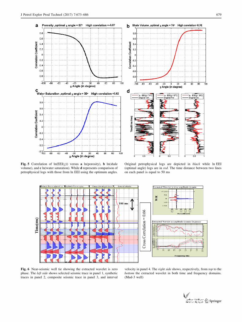
Fig. 5 Correlation of ln(EEI(v)) versus a ln(porosity), b ln(shale

volume), and c ln(water saturation). While d represents comparison of

petrophysical logs with those from ln EEI using the optimum angles.

Original petrophysical logs are depicted in black while ln EEI

(optimal angle) logs are in red. The time distance between two lines

on each panel is equal to 50 ms

Fig. 6 Near-seismic well tie showing the extracted wavelet is zero

phase. The left side shows selected seismic trace in panel 1, synthetic

traces in panel 2, composite seismic trace in panel 3, and interval

velocity in panel 4. The right side shows, respectively, from top to the

bottom the extracted wavelet in both time and frequency domains.

(Mud-3 well)

J Petrol Explor Prod Technol (2017) 7:673–686 679

123

impedance model is modified iteratively so as to make

better its fit with seismic trace. With a good initial model,

model-based inversion can be able to remove wavelet as

well as turning effects.

Low-frequency building

In order to create a low-frequency model, a set of auto-

matic horizons was generated, following the same proce-

dure as Pauget et al. (2009).

Two control horizons, manually interpreted (Fig. 8a),

were used to refine the generated automatic horizons so

that they follow the stratigraphy accurately (Fig. 8b).

Acoustic and gradient impedance logs from different wells

were interpolated along the mapped horizons with accurate

stratigraphic control, as shown in Fig. 8c (acoustic impe-

dance). Finally, the interpolated model was filtered in the

0–10-Hz low-frequency range (Fig. 8d). With respect to

this study, the inverse distance-based algorithm was

applied for the interpolation, and hence the detailed back-

ground models were obtained. A total of 4 wells were used

to build three background models (AI, GI, and Vp), from

which the inversion started.

Statistical/quantitative wavelet extraction and synthetic

seismogram

Prior to the inversion, near-, mid-, and far partial stacks

were used to conduct seismic well tie. This is achieved by

comparing the real and synthetic seismic data in the time

window of interest (500 ms was used herein). The time–

depth relationship at each well was available, which

permitted an extraction of statistical wavelet in the target

interval. The extracted statistical wavelet was then used to

build a synthetic data. The correlation coefficient between

the latter data and the real near seismic was improved

from 0.4 to 0.5 by applying a wavelet phase rotation, and

therefore the time–depth relationship was updated.

Finally, the correlation coefficient was improved again up

to 0.6 after using well data (Vp, Vs, and density logs). The

process consists of creating a reflectivity from Vp, Vs, and

density logs using Zoeppritz equation or its approxima-

tions, convolving it with the previous rotated wavelet to

generate the synthetic seismic traces, then the wavelet

(especially the phase) and time–depth relationship is

iteratively updated so that the synthetic seismic traces fit

pretty well the real seismic data as shown in Figs. 6 and 7.

Fig. 7 Far-seismic well tie showing the extracted wavelet is zero

phase. The left side shows selected seismic trace in panel 1, synthetic

traces in panel 2, composite seismic trace in panel 3, and interval

velocity in panel 4. The right side shows, respectively, from top to the

bottom the extracted wavelet in both amplitude and frequency

domains (Mud-3 well)

Table 1 Seismic data QC and conditioning

Step Check/not check QC results

Zero-phase QC Check All three seismic cubes are zero phase (Figs. 5, 6)

Time shift QC Check Far section is time-shifted to about -6 ms (correction was applied)

Frequency and phase balancing Check Well balanced

680 J Petrol Explor Prod Technol (2017) 7:673–686

123

Quality control on wavelets showed that it is stable up to

the frequency of 55 Hz, and the correlation coefficients

are acceptable.

Once the edited time–depth relationship is produced for

each well and the optimum seismic wavelets are extracted,

it becomes then straightforward to invert seismic data.

Three wells in the target area were used to constrain the

inversion results by cross plotting ln AI versus ln GI in one

hand, and ln AI versus ln Vp in the other hand. Linear

trends obtained from those relationships were then used for

the inversion regularization.

Seismic inversion results and QC

Figure 9 shows the section view of acoustic and gradient

impedance inversion results produced by this approach.

The section passes through 3 wells depicted by gamma ray

logs (black curve on each section). Mud-1 well was omitted

in the inversion process to serve as a blind test well, and the

rest wells were used to generate the low-frequency back-

ground model. Considering the 4 wells used in this study,

including Mud-1 well (blind test well), the correlation

coefficients between the inverted and the initial logs were

Fig. 8 Generation of low-frequency models used in the inversion:

a control horizons delimiting the target and used to refine the

generated automatic horizons, b numerous generated auto-tracked

horizons following the stratigraphy, c interpolation of elastic prop-

erties along the auto-tracked horizons, d filtering and generation of

low-frequency model

Fig. 9 Sections passing though

wells showing the inverted

acoustic impedance (a) andgradient impedance (b). Theoverlain black curves on the

sections are GR logs

J Petrol Explor Prod Technol (2017) 7:673–686 681

123

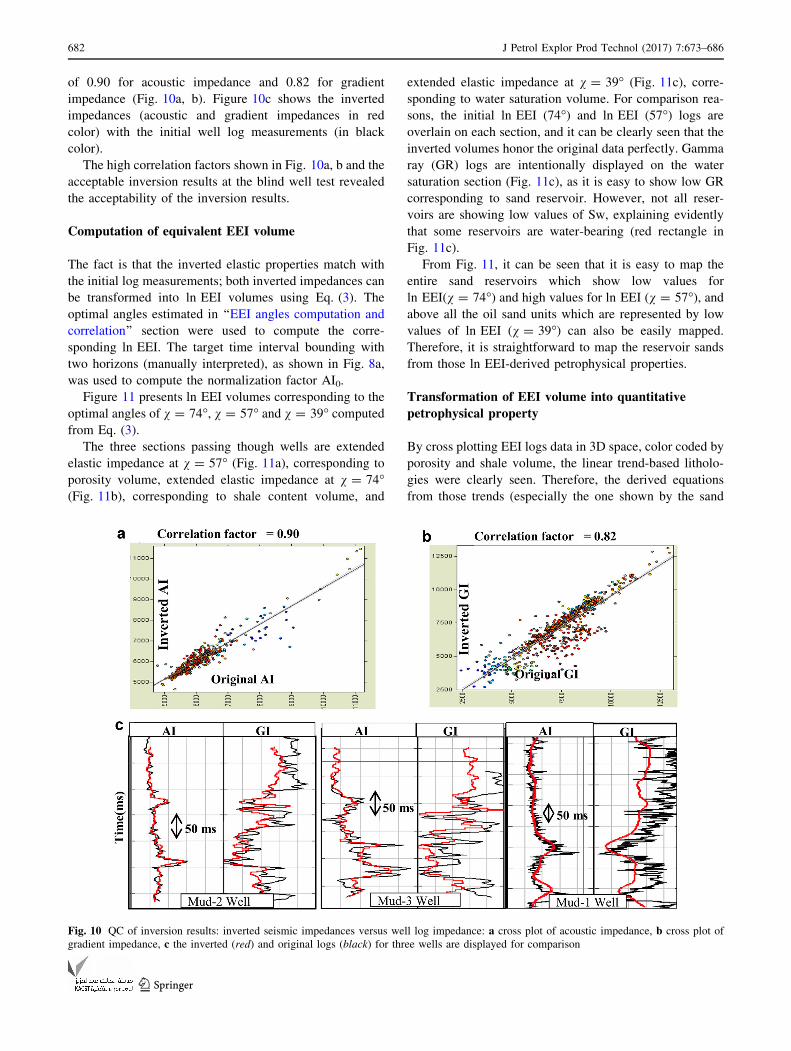
of 0.90 for acoustic impedance and 0.82 for gradient

impedance (Fig. 10a, b). Figure 10c shows the inverted

impedances (acoustic and gradient impedances in red

color) with the initial well log measurements (in black

color).

The high correlation factors shown in Fig. 10a, b and the

acceptable inversion results at the blind well test revealed

the acceptability of the inversion results.

Computation of equivalent EEI volume

The fact is that the inverted elastic properties match with

the initial log measurements; both inverted impedances can

be transformed into ln EEI volumes using Eq. (3). The

optimal angles estimated in ‘‘EEI angles computation and

correlation’’ section were used to compute the corre-

sponding ln EEI. The target time interval bounding with

two horizons (manually interpreted), as shown in Fig. 8a,

was used to compute the normalization factor AI0.

Figure 11 presents ln EEI volumes corresponding to the

optimal angles of v = 74�, v = 57� and v = 39� computed

from Eq. (3).

The three sections passing though wells are extended

elastic impedance at v = 57� (Fig. 11a), corresponding to

porosity volume, extended elastic impedance at v = 74�(Fig. 11b), corresponding to shale content volume, and

extended elastic impedance at v = 39� (Fig. 11c), corre-

sponding to water saturation volume. For comparison rea-

sons, the initial ln EEI (74�) and ln EEI (57�) logs are

overlain on each section, and it can be clearly seen that the

inverted volumes honor the original data perfectly. Gamma

ray (GR) logs are intentionally displayed on the water

saturation section (Fig. 11c), as it is easy to show low GR

corresponding to sand reservoir. However, not all reser-

voirs are showing low values of Sw, explaining evidently

that some reservoirs are water-bearing (red rectangle in

Fig. 11c).

From Fig. 11, it can be seen that it is easy to map the

entire sand reservoirs which show low values for

ln EEI(v = 74�) and high values for ln EEI (v = 57�), andabove all the oil sand units which are represented by low

values of ln EEI (v = 39�) can also be easily mapped.

Therefore, it is straightforward to map the reservoir sands

from those ln EEI-derived petrophysical properties.

Transformation of EEI volume into quantitative

petrophysical property

By cross plotting EEI logs data in 3D space, color coded by

porosity and shale volume, the linear trend-based litholo-

gies were clearly seen. Therefore, the derived equations

from those trends (especially the one shown by the sand

Fig. 10 QC of inversion results: inverted seismic impedances versus well log impedance: a cross plot of acoustic impedance, b cross plot of

gradient impedance, c the inverted (red) and original logs (black) for three wells are displayed for comparison

682 J Petrol Explor Prod Technol (2017) 7:673–686

123

reservoir) were then used to convert the EEI volumes into

shale content, water saturation, and porosity volumes.

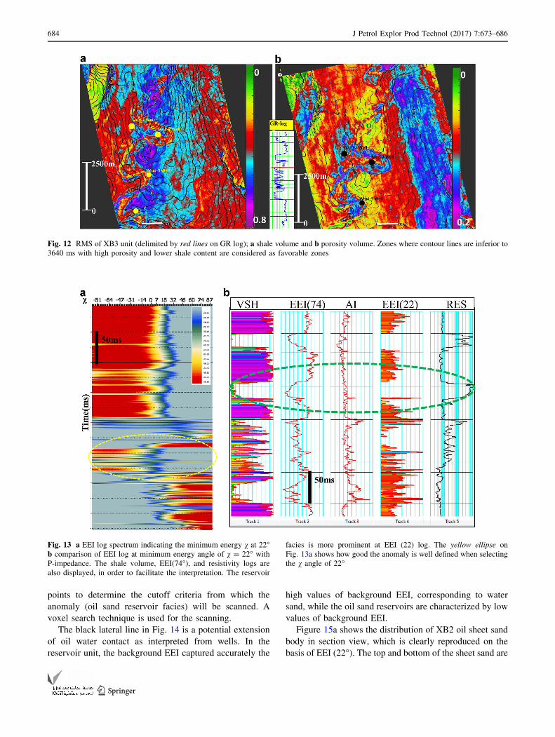
Figure 12a shows the RMS (root mean square) of porosity

map of the top and bottom of XB3 unit. Figure 12b shows

the RMS of shale content of the same unit. Zones where

contour lines are inferior to 3640 ms with high porosity

and lower shale content are favorable zones. The close

observation of Fig. 12a, b reveals that the reservoir is

clearly defined by shale volume. In addition, high values of

porosity map which should be related to the presence of

reservoir are also observable. In the east of the porosity

map, there is a quite big zone with very high values, which

geologically does not make sense to be a potential zone

insofar as the zone is in the low relief; thus, it can be

declared as a non-hydrocarbon potential zone.

Facies distribution

In order to obtain the reservoir facies distribution, the

concept of minimum energy v0 was applied on the entire

formation. The idea was also to isolate the oil reservoir

sand from the non-reservoir facies. After generating the

EEI log spectrum (angle ranging from v = -90� to

v = ?90�), the analysis of the spectrum was meticulously

carried out and the minimum energy angle was located at

exactly v = 22�, as shown in Fig. 13a. This conveys the

information that at v ¼ 22�, the non-reservoir beds (shale)

contrast poorly with each other in the log property; thus,

bodies highly contrasting within the background shale

could be seen and captured easily. That is why this angle is

considered as the minimum energy angle. The computed

EEI at this angle is also called the background EEI (Hicks

and Francis 2006).

A comparison between the background EEI with resis-

tivity and P-Impedance logs is shown in Fig. 13b, which

revealed that P-impedance log could not discriminate the

sand unit from the non-reservoir (green ellipse in Fig. 13b).

Moreover, the separation between the two lithologies

(shale for non-reservoir and sand for reservoir) is evident

(Fig. 14). To capture the oil sand reservoir facies, the

distribution of oil sand reservoir facies in background EEI

section, as shown in Fig. 15, was analyzed at well control

Fig. 11 ln EEI sections passing

though wells showing a ln EEI

at v = 57�, corresponding to

porosity volume, and b ln EEI

at v = 74�, corresponding to

shale content volume, and

c ln EEI at v = 39�,corresponding to water

saturation volume. Except the

last figure, corresponding

petrophysical properties derived

from well logs are overlain on

the two sections for comparison.

GR logs are intentionally plot

on the water saturation section,

as it is easy to show low GR

corresponds to sand reservoir.

However, not all reservoirs are

showing low values of Sw,

explaining evidently that some

reservoirs are water-bearing

(red rectangle)

J Petrol Explor Prod Technol (2017) 7:673–686 683

123

points to determine the cutoff criteria from which the

anomaly (oil sand reservoir facies) will be scanned. A

voxel search technique is used for the scanning.

The black lateral line in Fig. 14 is a potential extension

of oil water contact as interpreted from wells. In the

reservoir unit, the background EEI captured accurately the

high values of background EEI, corresponding to water

sand, while the oil sand reservoirs are characterized by low

values of background EEI.

Figure 15a shows the distribution of XB2 oil sheet sand

body in section view, which is clearly reproduced on the

basis of EEI (22�). The top and bottom of the sheet sand are

Fig. 12 RMS of XB3 unit (delimited by red lines on GR log); a shale volume and b porosity volume. Zones where contour lines are inferior to

3640 ms with high porosity and lower shale content are considered as favorable zones

Fig. 13 a EEI log spectrum indicating the minimum energy v at 22�b comparison of EEI log at minimum energy angle of v = 22� withP-impedance. The shale volume, EEI(74�), and resistivity logs are

also displayed, in order to facilitate the interpretation. The reservoir

facies is more prominent at EEI (22) log. The yellow ellipse on

Fig. 13a shows how good the anomaly is well defined when selecting

the v angle of 22�

684 J Petrol Explor Prod Technol (2017) 7:673–686

123

shown, respectively, by two horizontal lines on GR log.

Figure 15b is the 3D view of the sheet sand where contour

lines are also displayed, and it can clearly be seen that the

sheet sand body conforms to the structure. Figure 15c

shows the 3D distribution of lower reservoir sand bodies,

as shown by blue and orange colors painted on GR log,

captured using both porosity and shale volume cubes.

Conclusion

1. Extended elastic impedance (EEI) concept allowed us

to characterize reservoir properties in the Nianga field

through quantitative estimates of reservoir properties.

This was achieved by identifying the optimum EEI

angle corresponding to each petrophysical property

based on well log data. Three reservoir properties:

porosity (/), water saturation (Sw), and shale volume

(Vsh) show high correlation with ln EEI logs at

v = 57�, 39� and 74�, respectively.2. In order to obtain the reservoir facies distribution, a

background EEI was established based on an identified

minimum energy angle, thereby enabling the mapping

of reservoir facies from quantitative petrophysical

properties and background EEI cubes.

3. This concept has proved to be more successful than

conventional acoustic impedance approach especially

with regard to fluid and lithology discrimination.

Fig. 14 A section passing

though wells showing extended

elastic impedance at v ¼ 22�

corresponding to the

background EEI

Fig. 15 a XB2 sheet sand body distribution clearly reproduced on thebasis of EEI (22�) while GR log on the figure shows the top and

bottom of the sheet sand. b View of the sheet sand body in 3D space.

Contour lines are also displayed, and it can clearly be seen that the

sheet sand body conforms to structure. c XB3pcf channel and sheet

sand body distribution clearly reproduced

J Petrol Explor Prod Technol (2017) 7:673–686 685

123

Hence, it can be applied for the purpose of mapping

favorable zones that may suggest possible future

drilling locations.

4. The porosity and shale volume derived herein provided

a superior description of reservoir sand. The EEI-based

porosity agreed with the regional depositional trend of

the Congo basin and provide and enhanced lateral

distribution of the geological facies.

Open Access This article is distributed under the terms of the

Creative Commons Attribution 4.0 International License (http://

creativecommons.org/licenses/by/4.0/), which permits unrestricted

use, distribution, and reproduction in any medium, provided you give

appropriate credit to the original author(s) and the source, provide a

link to the Creative Commons license, and indicate if changes were

made.

References

Archie GE (1942) The electrical resistivity log as an aid in

determining some reservoir characteristics. Trans Am Inst Mech

Eng 146:54–62

Avseth P, Mukerjo T, Mavko G (2005) Quantitative seismic

interpretation—applying rock physics tools to reduce interpre-

tation risk. Cambridge Press, ISBN 0-539-81601-7. Cambridge

University Press

Avseth P, Veggeland T, Christiansen M, Lrdal KJ, Horn F (2013)

Pseudo-elastic impedance calibrated to rock physics models for

efficient lithology and fluid mapping from AVO data. In: Paper

presented at the 75th EAGE conference & exhibition incorpo-

rating SPE EUROPEC

Bachrach R (2006) Joint estimation of porosity and saturation using

stochastic rock-physics modeling. Geophysics 71:53–63

Ball V, Blangy JP, Tenorio L (2013) Statistical aspects of rock

property depth series: the trend is not your friend. In: Paper

presented at the 83rd annual international meeting, SEG,

expanded abstracts

Ball V, Blangy JP, Schiott C, Chaveste A (2014) Relative rock

physics. Lead Edge 33:276–286. doi:http://dx.doi.org/10.1190/

tle33030276.1

Chatterjee R, Gupta SD, Farroqui MY (2013) Reservoir identificarion

using full stack seismic inversion technique: a case study from

Cambay basin oilfields, India. J Pet Sci Eng 109:87–95. doi:10.

1016/j.petrol.2013.08.006

Connolly P (1999) Elastic impedance. Lead Edge 18:438–452. doi:10.

1190/1.1438307

Dong W (1996) A sensitive combination of AVO slope and intercept

for hydrocarbon indication. In: Paper presented at the 58th

conference and technical exhibition, Eur. Assn. Geosci. Eng,

Paper M044

Doyen PM (2009) Porosity from Seismic data: a geostatistical

approach. Geophysics 53:3963–3975

Dubucq DB, Van Riel S (2001) Turbidite reservoir characterization:

multi-offset stack inversion for reservoir delineation and porosity

estimation; aGulf ofGuineaexample. In: Paper presented at the71st

annual international meeting, Soceity of Exploration geophysics

Hampson D, Russell B, Bankhead B (2005) Simultaneous inversion

of pre-stack seismic data: SEG. Expand Abstr 24(1):1633–1637

Hicks G, Francis A (2006) Extended elastic impedance and its

relation to AVO cross ploting and Vp/Vs. In: Paper presented at

the EAGE extended abstract

Hodrick RJ, Prescott EC (1997) U. S. business cycles: an empirical

investigation. J Money Credit Bank 29:1–16

Mavko G, Mukerji T, Dvorkin J (1998) The rock physics handbook:

tools for seismic analysis in porous media. Cambridge Univer-

sity Press, Cambridge

Morteza Amiri JG-F, Golkar B, Hatampourd A (2015) Improving

water saturation estimation in a tight shaley sandstone reservoir

using artificial neural network optimized by imperialist compet-

itive algorithm—a case study. J Pet Sci Eng 127:347–358.

doi:10.1016/j.petrol.2015.01.013

Pauget F, Lacaze S, Valding T (2009) A global approach to seismic

interpretation base on cost function and minimization. In: Paper

presented at the 79th annual international meeting, SEG,

Expanded abstracts

Romero CE, Carter JN (2001) Using genetic algorithms for reservoir

characterisation. J Pet Sci Eng 31:113–123. doi:10.1016/S0920-

4105(01)00124-3

Sams MS, Millar I, Satriawan W, Saussus D, Bhattacharyya S (2011)

Integration of geology and geophysics through geostatistical

inversion: a case study. First Break 29:47–56

Sengupta M, Bachrach R (2007) Uncertainty in seismic-based pay

volume estimation: analysis using rock physics and Bayesian

statistics. Lead Edge 26:184–189

Thomas M, Ball V, Blangy JP, Davids A (2013) Quantitative analysis

aspects of the EEI correlation method. In: Paper presented at the

83rd annual international meeting, SEG, Expanded abstracts

Vernik L, Fisher D, Bahret S (2002) Estimation of net-to-gross from P

and S impedance in deepwater turbidites. Lead Edge 21:380–387

Whitecombe DA, Connolly PA, Reagan RL (2002) Extended elastic

impedance for fluid and lithology prediction. Geophysics

67:63–67

Wiggins R, Kenny GS, McClure CD (1983) A method for determin-

ing and displaying the shear-velocity reflectivities of a geologic

formation. European Patent Application 83300227.2, Bull.

84/30, July 25

686 J Petrol Explor Prod Technol (2017) 7:673–686

123