reservoir innovations - halliburton.com · the reservoir sediments, comprising alternations of...

ReseRvoiR innovations

I n T h I s I s s u e

Real-Time Reservoir Characterization and Geosteering Using Advanced High-Resolution LWD Resistivity ImagingSee pages 4-10

Optimizing VSP Anisotropy Surveys with Reflection Data See pages 30-32

VOLUME 3, NO. 2, 2014 A FORMATION EVALUATION TECHNOLOGY JOURNAL

2

A Message from Ian Hunt and Mac UpshallWelcome to the sixth edition of ReseRvoiR innovations. This technology journal is filled with valuable information on formation and reservoir evaluation solutions that increase reservoir understanding, and add value to our customers’ workflows. This issue includes recent major industry papers coauthored by Halliburton specialists and our clients, through industry organizations such as the SPE and SPWLA.

Understanding our customers’ needs, proposing and applying technical solutions to solve our customers’ challenges and increasing the asset value is at the heart of everything Halliburton does. To facilitate this process and enhance the organizational capability in each business unit, Halliburton has created a new Technical Sales family. The teams that work in this new structure are technical and solution experts. They have the experience, capability and desire to engage our customers with a dialogue to address their reservoir challenges. The papers written in this edition are a testament to this new organization, and we are committed to continue building these strong teams and enhancing their effectiveness and credibility in the industry.

For example, one of our paper selections, “Investigating the Dynamic Three-Dimensional Loading Effects on Perforating Guns Imposed by Shaped Charges” explores how Halliburton developed a 3D simulation and hydro model to help understand the complicated interactions between explosives, fragmented casings, and the gun wall during a perforating event. Traditional gun design approaches and standards use collapse pressure calculation and swell measurement with overloaded charges as design verification methods. In this paper, a new design model is presented that augments traditional design approaches and provides gun designers with better data on gun system structural performance, including the effects of phasing, shot density, and charge type.

A second example, “Real-Time Reservoir Characterization and Geosteering Using Advanced High-Resolution LWD Resistivity Imaging” describes the advances in LWD electrical imaging that, in addition to providing reservoir characterization, can also provide real-time fracture identification, dip picking and geosteering information, all of which can be used to place the wellbore optimally in the reservoir to maximize production.

We encourage you to collaborate with our Technical Sales and Formation and Reservoir Solutions representatives to coauthor future papers that highlight solutions to your reservoir challenges. We welcome your interest and feedback in our publications and we sincerely hope you find them both valuable and enjoyable.

Thank you,

Ian R. Hunt Mac UpshallSales & Marketing Director, Global Technical Sales & Wireline and Perforating Marketing Manager, Sperry Drilling

Executive Steering CommitteeEric CarreSenior Vice President, Drilling & Evaluation

David ToppingVice President, Wireline and Perforating

Ahmed KenawiVice President, Sperry Drilling

Greg PowersVice President, Technology

Editorial Advisory CommitteeRoland Chemali Ron Cherry Daniel Dorffer Ian R. Hunt Andrew Kirkwood Dan Quinn Sriram Srinivasan Mac UpshallRon Dirksen Paul CooperTim ParkerJoe Zuiker

Managing EditorsSoraya Brombacher Roselle Mohle

CirculationNancy Kirkland Steven Thrift

DesignGriffin Creative Company

This magazine is published biannually by Halliburton Wireline and Perforating and Sperry Drilling.

For comments and suggestions, contact: [email protected] or [email protected].

On the CoverDynamic, interactive and intuitive geosteering is the key to accurate wellbore positioning.

The ADR™ azimuthal deep resistivity sensor provides deep reading (up to 18 feet into the formation), directional, and high-

resolution images that give early warning of approaching bed boundaries before the target zone is exited. Also a traditional multi-frequency compensated resistivity sensor—this one tool provides over 2,000 unique measurements for both precise wellbore placement and more accurate petrophysical analysis.

© Copyright 2014 Halliburton. All rights reserved.

3

Contents

4 Real-Time Reservoir Characterization and Geosteering Using Advanced High-Resolution LWD Resistivity Imaging

AFR™ Sensor High-Resolution Resistivity Imaging

11 Characterizing a Turbiditic Reservoir Determining Resistivity Anisotropy for Laminated Reservoir Analysis

18 Milestone in Production Using Proactive Azimuthal Deep Resistivity Sensor Combined with Advanced Geosteering Techniques: Tarapoa Block, Ecuador

Maintain the Well in the Sweet Spot

26 Locating Bypassed Reserves in Geologically Complex Mature Field Environments

Azimuthal Deep-Reading Resistivity for Complex Reservoir Evaluation

30 Optimizing VSP Anisotropy Surveys with Reflection Data Cost-Effective Advances in Survey Design Analysis

33 Evaluation of General Resistivity Density-Based Saturation in Thin, Laminated Sand-Shale Sequences

Enhanced Hydrocarbon Recovery with Multicomponent Induction Tool

39 Investigating the Dynamic Three-Dimensional Loading Effects on Perforating Guns Imposed by Shaped Charges

Shaped Charge Loading Effects on Guns

45 Integrated Formation Evaluation of Tight Gas Delineation Wells: Best Practices and Lessons Learned

Data Integration to Better Understand Reservoir Behavior

4

11

26

30

33

39

45

18

4

Real-Time Reservoir Characterization and Geosteering Using Advanced High-Resolution LWD Resistivity ImagingNedhal Al-Musharfi, Radhey Bansal, Mahbub Ahmed, and Mazen Kanj, Saudi Aramco; Marian Morys, Chris Conrad, Roland Chemali, Amr Lotfy, Mohammed Bayrakdar, and Tim Parker, Halliburton Sperry Drilling

This paper was presented at the SPE Annual Technical Conference and Exhibition held in Florence, Italy, 19–22 September 2010.Copyright 2010 Society of Petroleum Engineers. Reproduced with permission of the copyright owner.

Further reproduction prohibited without permission.

AbstractA recently introduced azimuthal resistivity LWD imaging tool has been upgraded with advanced high-resolution sensors that are capable of differentiating reservoir and borehole features down to a size of 0.4-in. when drilling in well consolidated formations. The high vertical and azimuthal resolution, along with 100% borehole coverage, yield an image quality comparable to that of wireline service for applications that include fracture characterization and formation evaluation.

This paper describes a field test of the high-resolution tool in 5 7⁄8-in and 8 3⁄8-in holes in Saudi Arabia and shows the application of LWD images for estimating carbonate reservoir producibility involving the characterization of secondary porosity. The LWD imager provides significant economic and logistic benefits, especially in slim horizontal sections; in addition, it can identify fractured zones with mud loss potential shortly after penetration. The real-time resistivity provides a good basis for accurate dip calculation and geosteering in general.

In its default configuration, the high-resolution tool is equipped with six high-resolution sensors arranged in two rows. One of the benefits of the multi-sensor configuration, demonstrated by the field test, is the ability to validate the image quality by comparing data from various sensors. Another benefit is the depth correction achieved by correlating images from identical sensors located at various depths.

The paper also discusses the fundamental principles behind high-resolution resistivity imaging in conductive mud and makes extensive use of modeling techniques to characterize the sensor performance in various practical situations.

IntroductionCarbonate reservoirs from the producing oil and gas fields in Saudi Arabia have extreme ranges of porosity and permeability, both laterally and vertically (Ehrenberg, Nadeau, and Aqrawi, 2007). These ranges of variation in reservoir properties have made the reservoirs highly heterogeneous. The degree of heterogeneity further increases toward the flank of the structures, where the prediction of lateral reservoir continuity presents a major challenge to the geoscientists. The incremental oil and gas recovery from such heterogeneous reservoirs through horizontal wells has been found to be favorable. Consequently, Saudi Aramco has undertaken an ambitious horizontal drilling program for incremental oil and gas recovery.

This paper describes two important carbonate reservoirs of Saudi Arabia: a gas carbonate reservoir in the Upper Permian formation, a deep-seated non-associated gas-producing reservoir, and an oil carbonate reservoir in the Upper Jurassic formation, a prolific oil-producing reservoir. The azimuthal focused resistivity LWD imaging tool was tested in these reservoirs to help characterize them in finer detail and to enable the team to take proactive actions to maintain the bit in the desired part of the reservoir while geosteering horizontal wells.

The resistivity images provided an important component of the reservoir characterization and contributed to real-time geosteering decisions. They were obtained from a novel LWD azimuthal focused resistivity sensor array (Prammer et al. 2007). The array was recently upgraded to deliver some of the images in a

AFR™ SENSOR HIGH-RESOLUTION RESISTIVITY IMAGING

higher-resolution. Although the resolution gain was partially lost to the mud pulse telemetry, the well placement was successful, and the full benefit of the higher-resolution was realized in post-well analyses once the high-density on-board memory data became available to the geoscientists.

A detailed description of the sensor array and its upgrade showing the benefits and limitations of the improved design is provided in this paper. Some additional benefits of the new array design, including image quality control and compensation for irregular tool motion, are also discussed and illustrated.

Stratigraphic Context and Facies DevelopmentThe gas carbonate formation represents an epeiric carbonate platform that developed above the siliciclastics of the Unayzah formation and its equivalents after the middle Carboniferous (Hercynian) orogeny and the middle Permian rifting (Sharland et al. 2001). The gas carbonate formation consists of five depositional sequences A, B, C, D, and E, in descending stratigraphic order, deposited during the Upper Permian time (Fig. 1).

The reservoir sediments, comprising alternations of carbonates and anhydrate, were deposited in a shallow open marine to tidal flats environment. The reservoir development within the reservoir sediments is evident in the sequence-A, B, and C depositional sequences, but sequence-C largely forms the primary reservoir developed throughout the study area; it contributes greatly to the non-associated gas production of Saudi Arabia. Sequence-C reservoir facies are highly heterogeneous, thin, and discrete, as a result of the varied depositional environment and diagenetic changes. Parts of the reservoir facies have been dolomitized and later leached, which resulted in good reservoir development. Some dolograinstone facies, however, have been cemented by anhydrite, which reduced the reservoir porosity.

The other formation of interest is the oil carbonate formation. It consists of four regionally correlative depositional sequences of carbonate capped by evaporite, termed as A, B, C, and D in descending order (Fig. 2). The reservoir development is evident in all four depositional sequences, but sequence-D is the main oil-producing reservoir.

Sequence-D formation has thickness in hundreds of feet, prolific porosity development, and permeability of up to several Darcy, and on a finer scale, it can be further subdivided into four major shoaling-upward

5

carbonate cycles. The upper half is dominated by exceptionally high reservoir-quality facies composed of skeletal grainstones and packstones with ooid grainstones.

The lower half contains interbeds of high and relatively low to non-reservoir-quality facies (Lindsay et al. 2006). The diagenetic processes that have affected sequence D reservoir include dolomitization, leaching, recrystallization, cementation, compaction, and fracturing. Moldic to intergranular porosities are common. Microporosity is also found in abundance in both limestone and dolomite lithology, and accounts for between 25 to 50% of the total porosity (Cantrell and Hagerty, 1999).

The horizontal wells are primarily placed in the sequence-D1 and D2 reservoir facies. By contrast, the reservoir facies near the lower part of sequence-D2 are avoided as they possess abnormally high permeability and could provide a conduit for water breakthrough. Geosteering with images from the azimuthal density and from the azimuthal focused resistivity is aimed at maintaining the well path in the characteristic reservoir facies of sequence-D1 and upper part of sequence-D2, and avoiding entering the lower part of sequence-D2.

The LWD Azimuthal Focused Resistivity Sensor ArrayElectrical images have long been recognized as the preferred measurement for characterizing geological facies (Serra et al. 1993). Laminations, fractures, unconformities, vugs, slumps, formation boundaries, changes in lithology, and many other geological features are easily recognized and described in detail. Initially, electrical images were produced by sophisticated wireline instruments. More recently, through advances in technology, it has become possible to acquire electrical images while drilling. The azimuthal focused resistivity tool discussed in this paper, for example, is capable of scanning the surface of the wellbore with multiple imaging sensors sampled up to 128 times per revolution of the bottomhole assembly (BHA). The instrument was described in the open literature in its original implementation (Prammer et al. 2007).

Fig. 3 shows the general layout of the sensor array. The array consists of three rows of three current electrodes each, and is affixed to an electrically activated section of the drill collar. The section is energized by two symmetrically located toroidal transmitters. The three rows of microresistivity sensors rotate with the BHA and cover the borehole

Figure 1. Generalized Paleozoic stratigraphic columns in Saudi Arabia showing the stratigraphic position of the Permian formations on the left, and vertical stacking of the reservoir developed within the gas carbonate formation on the right.

Figure 2. Generalized Paleozoic stratigraphic columns in Saudi Arabia showing the stratigraphic position of the Upper Jurassic formations on the left, and reservoir facies developed with sequence-D on the right. Sequence-1 and 2 are the primary producing reservoir facies within sequence-D.

Figure 3. The azimuthal focused resistivity LWD array includes two transmitting toroids and three rows of three azimuthally spaced microresistivity sensors for electrical imaging. In the standard original configuration, each microsensor has a nominal pixel resolution of 1-in. In the upgraded high resolution version, some of the microsensors have a nominal pixel resolution of 0.4-in.

6


Figure 4. Expected pixel resolution of the image as a function of the sensor electrode size and of the magnitude of the standoff. The pixel resolution is selected as the size of the feature for which the resistivity reading reaches 90% of the expected value.

circumference in its entirety. A resistivity map is derived by representing the measurements of the microsensors and is displayed as an electrical image.

One of the salient features of the array shown in Fig. 3 is the symmetry of the transmitters and microsensor assemblies around the midpoint. Another relevant feature is the redundancy presented by nine different sensors covering the surface of the borehole in sequence. The symmetry of the array around its midpoint helps to ensure an accurate representation of the geological features, whereas a non-symmetrical array would produce non-symmetrical image artifacts. The redundancy of the sensors presents multiple benefits. First, it enables full coverage of the borehole surface over a wide range of RPM/rate of penetration (ROP) ratios. Redundancy also improves the signal-to-noise ratio. Finally, the redundancy can be used for log quality control and to estimate the actual ROP of the BHA independently of the depth measurement at the surface.

Electrical images are recorded in the tool memory during drilling or wiping the hole. The memory is downloaded when the BHA is returned to the surface. Memory images preserve the quality and detail of the original images, but are available only at the end of a run. In real time, only one image of lower-resolution is generally pulsed to the surface. This image plays an important role in recognizing the geology and the facies. The geological information, although of lower-resolution, is critical for some real-time decisions, particularly those related to geosteering. Clearly, the limitation in resolution and number of real-time images is related to mud pulse telemetry rates. When wired pipe telemetry is available, multiple high-resolution images can be acquired and sent to the surface as the bit drill through the formation.

Since its first release in 2007, the azimuthal focused resistivity sensor array has been upgraded to acquire some of the images in higher-resolution. From the outside, the original instrument and the upgraded instrument look very similar (Fig. 3). The upgraded high-resolution version retains the same general configuration, but some of the rows of sensors are equipped with smaller dimension-sensing buttons that yield a pixel resolution of about 0.4-in. The original microsensors were specified with a pixel resolution of 1-in. This increase in resolution has come at the cost of a reduced signal/noise ratio in very high resistivity, because the sensing

current emitted by the new buttons is significantly smaller. From a practical standpoint, a compromise was adopted. Some of the button rows are high-resolution with a 0.4-in pixel size, but are limited to resistivity values of hundred ohms or less; the other button rows retained the original resolution of 1 pixel and remain capable of measuring resistivity values of several thousand ohm-m. The sampling rate was significantly increased to realize the benefit of a higher-resolution microsensor.

The improved pixel resolution requires that sensor electrodes feature a smaller contact area with the borehole fluid, as shown in Fig. 3; it also requires a closer fit between the outer diameter of the sensor carrier and the diameter of the wellbore. The surface area of the microsensors and the magnitude of the standoff from the borehole wall play determinant roles in governing the resolution of the image. Stated briefly, a large area sensor electrode rotating very closely to the borehole wall yields a poor resolution image. Similarly, a small area sensor operating far from the borehole wall also yields a poor resolution image. Fig. 4 shows the combined effect of sensor electrode size and standoff on the resolution of the image. The results were derived through 3D computer modeling.

Data Quality Control Using Multi-Image Capability of Azimuthal Focused ResistivityIn many instances, micro-electrical images include small random features that may appear as noise superimposed on the signal. For the geoscientist studying the images, these random features can be interpreted as real micro-events, faithfully describing the formation, or they can be simply dismissed as artifacts created by electronic noise or by vibration-related stray signals. Clearly,

the difference between random noise and real micro-events is very important from the geological interpretation standpoint. Features that can be mistaken for noise include small nodules of pyrite, vugs, microfractures, or calcite cementation. Vugs and microfractures in particular account for the secondary microporosity. By using the redundancy between the various sensors, these small events can be positively confirmed or invalidated. The method relies on the fundamental observation that the individual images from the various microsensors are acquired at different times. Any feature that displays on two separate images must therefore be real; a feature that displays on only one image should be interpreted as noise. This criterion was applied to multiple logs and has helped to validate those that would otherwise have been considered as faulty (Fig. 5).

Determining ROP Based on Image CorrelationThe time delay between the acquisitions of various images by the azimuthal focused resistivity instrument can be applied to the computation of the actual ROP. This capability is particularly useful when using an automatically controlled drilling rig sometimes designated as an “auto-driller.” In Fig. 6, the rig operator relies on a robotic drilling apparatus that regulates the weight at the top drive to remain within prescribed upper and lower limits. The top drive is held back when the apparent weight on bit reaches the upper limit, and then is released to move down when the apparent weight on bit reaches the lower limit. This results in an irregular depth metering by the surface depth encoder. Because LWD image acquisition relies on the time-depth relationship from the depth encoder, the resulting image exhibits the jagged appearance shown on the left image of Fig. 6. It was postulated that the jagged look occurred as a result of the mismatch between the depth measured at the surface and a probable smooth progression of the BHA. Simply smoothing the time-depth relationship dramatically improved the image appearance, as shown on the right image of Fig. 6.

A more exact method for quantifying the progress of the drill string uses the similarity between the images acquired by longitudinally spaced sensors. On Fig. 3, the image acquired by the upper transmitter and its nearest row of microsensors is spaced by a fixed distance from the image acquired by the lower transmitter and its nearest row of microsensors. Conversely, the upper transmitter array and the lower transmitter array scan any given portion of the borehole wall at different times. By

7

Figure 5. Each of the two examples compares images acquired by the upper transmitter array and by the lower transmitter array respectively. The upper and lower transmitter images are typically acquired several minutes apart. Some of the micro-events have been circled. Their repeatability demonstrates that they are the result of real geological features, rather than noise.

Figure 6. When the depth measurement at the surface does not match the actual downhole progression of the LWD sensor, artifacts appear on the electrical image. In the example on the left, an automatic driller regulates weight on bit by intermittently releasing the drill string. The image features jagged boundaries. These artifacts are removed by smoothing the time-depth relationship, as shown on the right.

Figure 7. The apparent rate ROP derived from the depth encoder exhibits cyclical variations characteristic of the auto-driller mechanism. An independently computed ROP, based on image correlation, suggests a smooth true ROP. Corrections to the ROP, also based on image correlation, compensate for the cyclical error in the apparent ROP.

applying a cross-correlation algorithm between the two images, the time interval between them is determined and an average ROP is automatically computed. The cross-correlation method was applied to a log in which an auto-driller was used, and Fig. 7 shows the results. The ROP derived from the surface encoder exhibits a cyclical behavior typical of this type of drilling method. An independent computation of the ROP using an image-based correlation suggests a more regular ROP of the BHA. A calculation of the correction to the encoder shows the same cyclical behavior, and confirms the approach adopted in Fig. 6 of assuming a smooth ROP downhole.

Example 1: Well-A in the Gas FormationBy many accounts, the gas carbonate reservoir is considered to be geologically complex (Al-Fawwaz et al. 2007; Ameen et al. 2010). This reservoir is the earliest major carbonate sedimentation of the field and was deposited in shallow open marine to tidal flat environments. As shown in Fig. 1, the gas carbonate formation consists of five depositional sequences A, B, C, D, and E, in descending stratigraphic order. The primary reservoir unit, sequence-C, consists of grainstones and packstones, and interbedded mudstone to wackstone facies.

Fractures occur frequently in this reservoir and, although they contribute to production, they are not the dominant factor in reservoir performance. This fracture information was not known in the early development phase. Horizontal wells were initially oriented at high angles to the strike of the dominant natural fractures and maximum horizontal stress to maximize the interception of the natural fractures. When the contribution from fractures was determined to be non-critical, the wells were steered instead parallel to the maximum horizontal stress, i.e., parallel to the dominant fracture strike. The benefit was improved wellbore stability. Imaging the fracture trend helps to geosteer the well accordingly.

Fig. 8 shows three electrical images from Well-A drilled in the gas carbonate formation. The bottom image was acquired by the standard resolution microsensors (1-in. pixel) of the azimuthal focused resistivity. The two middle images were acquired by the high-resolution 0.4 in. microsensors. The “static” image corresponds to the data as acquired, with no additional image processing; the “dynamic” image was enhanced by histogram equalization. The image at the top of the figure provides a compressed view of the entire logged section.

8


Figure 9. Two separate images from Well-A at nearly 100 ft apart in measured depths show the characteristic “frowning” pattern of drilling down structure. These images are from recorded data in the on-board memory; they help to illustrate the bed layering in the reservoir. Lower resolution, real-time images are used to compute the relative dip and to make informed geosteering decisions.

Figure 8. Three images are shown for the same interval in Well-A. The best image is the high resolution dynamic image, with a pixel size of 0.4-in. Some partial fractures may be drilling induced. Their orientation parallel to the natural fracture confirms the stress field direction. The top of the figure shows a compressed image of the entire logged section.

Clearly, the high-resolution images provide finer detail and a more accurate picture of the subsurface. The primary fracture in particular is better shown in the high-resolution displays than in the standard resolution display. Smaller, incomplete fractures are clearly visible on the high-resolution dynamic display.

The primary natural fracture and the partial induced fractures are nearly parallel to one another, suggesting a well-defined in-situ stress direction. The well appears to be oriented at a somewhat high angle relative to the stress field.

In other sections of the well, the bedding can be clearly seen, nearly horizontal (Fig. 9) as the well progresses downdip. Two images acquired within a measured depth of 100 ft indicate a very high

relative angle. A software utility helps to quantify the magnitude of the relative dip. By combining the relative dip with the readings from the navigation sensor on the downhole assembly, a true dip calculation is performed with the same software. This application is particularly useful in real time for geosteering.

In other sections of the well healed fractures are observed terminating as they intersect anhydrite layers. These events suggest that the anhydrite may exhibit certain plasticity (Fig 10 a-b). Other fractures indicate a change in relative orientation of the in-situ with respect to the well path (Fig. 10c).

Example 2: Well-B in the Oil FormationFor Well-B of the oil carbonate sequence-D formation, the primary real-time applications of

micro-imaging while drilling included geosteering, identifying laminations and fractures for real-time decisions, and imaging borehole breakouts. Fig. 11 shows the geosteering application. The well path was near-horizontal. A real-time dip computation on the image provided a direct assessment of the relative dip, enabling real-time steering decisions.

The identification of lamination and fracture is very similar to that of Well-A. To illustrate an alternative display, Fig. 12 shows a 3D post-well view that indicates a fracture and some borehole breakouts. The fractures in this water-based environment are indicated by the darker shade, which corresponds to low resistivity. Similarly, borehole breakouts appear as dark-colored ridges.

The differentiation between open fractures and borehole breakouts are best illustrated in the 2D view of Fig. 13 in which the borehole breakout exhibits the characteristic shape and appearance. The relationship between borehole breakout and in-situ stress field has been extensively discussed in technical articles (e.g., Krabbe et al.1999).

Summary and ConclusionMicro-electrical images acquired while drilling have proven to be very valuable for real-time decisions and for formation evaluation in the gas and oil carbonate reservoirs. The higher-resolution images have helped to characterize the reservoir from many points of view, including fracture imaging and mapping for understanding the flow pattern and for recommending future well placement. Secondary porosity from vugs and large fractures is readily identified from high-resolution images stored in the tool memory. In-situ stress field orientation is readily derived from natural and induced fractures and from borehole breakouts. Laminations are defined with great accuracy, showing productive units, preferential flow direction, and potential permeability barriers. In real-time geosteering, decisions were guided by a lower-resolution image. By taking advantage of the particular design of the azimuthal focused resistivity instruments with multiple redundant rows of microsensors, it was possible in one instance to flag an irregular ROP and correct for it.

9

Figure 10. This example is from Well-A. High resistivity, probably healed fractures are evident in intervals (a) and (b). Multiple conductive fractures display in interval (c). Some of the fractures show complete sinusoids within the borehole, whereas others seem to terminate.

Figure 11. Geosteering of Well-B in the sequence-D was enabled by real-time micro-electrical images identifying the sinusoidal patterns with great accuracy. A software utility helped compute directly relative dip and true dip.

Figure 12. 3D view of a fractured interval of Well-B. The core-like sections from left to right represent a succession of side views of a 4-ft interval rotated in sequence by 90 degrees, providing an all-around perspective of the wellbore image. The red arrows point to a probable fracture shown from all four angles. The blue arrow indicates a likely borehole breakout.

Figure 13. 2D unfolded view of a borehole breakout in Well-B. This section of the well was drilled perpendicular to the in-situ maximum stress field.

Mahbub Ahmed is a petroleum engineering consultant with Saudi Aramco’s gas reservoir management department. His expertise includes reservoir management, gas field development, and reservoir simulation. Prior to joining Saudi Aramco in 2001, Mahbub worked as a senior reservoir engineer with the Occidental Oil and Gas Company in

Bakersfield, California; as a senior consultant with Geoquest in Denver, Colorado; as a senior engineer with Scientific-Software Intercomp in Denver, Colorado; and as a reservoir engineer with the Algerian National Oil Company (Sonatrach) in Algiers. Mahbub has conducted numerous reservoir simulation and engineering studies of oil and gas fields across the U.S., South America, and the Middle East. He received his BS degree in 1982 from the Institut Algerian du Petrole, Boumerdes, Algeria, and his MS degree in 1988 from the University of Oklahoma, Norman, Oklahoma, both in petroleum engineering. Mahbub is a member of the Society of Petroleum Engineers (SPE).

Nedhal Al-Musharfi is the reservoir description division head at Saudi Aramco. He holds a BSc in mechanical engineering from King Fahd University of Petroleum and Minerals, Dhahran, Saudi Arabia. Nedhal has authored and co-authored several technical papers and served on many technical teams. He started his career with

Schlumberger in 1994 as a wireline field engineer and had exposure to the drilling and measurements segment. In his career, he also worked at different posts including recruiting manager, field studies petrophysicist, and senior exploration petrophysicist.

Authors

Marian Morys is president of PetroMar Technologies, Inc. Marian has over 25 years of experience in development of geophysical instrumentation for extreme environments, including wireline and LWD formation evaluation tools based on electromagnetic, NMR, acoustic, and optical sensors. Among the positions he held previously are:

vice president of technology at Electro-Petroleum and technology director at Halliburton Technology Center in Exton (formerly NUMAR). Marian received his MS degree in electrical engineering from Warsaw Technical University in Poland and an MBA from Pennsylvania State University. He is a member of SPE and SPWLA and coauthor on many patents and publications.

Christopher Conrad is the engineering director of PetroMar Technologies, Inc. He started in the industry with Halliburton in 2000 through NUMAR Corporation, most recently serving as technology director of Halliburton’s Exton technology center. He has been a leading technical contributor in the research and development of numerous

formation evaluation wireline and LWD tools. Chris’ technology portfolio includes NMR, multi-component induction, resistivity imaging, and acoustic imaging. Chris holds a BS degree in computer engineering, and a Masters of Engineering in electrical engineering, both from the Pennsylvania State University, University Park, PA.

Roland Chemali is a Halliburton technology fellow and chief petrophysicist for Sperry Drilling; he has coauthored multiple papers and patents on formation evaluation. In 1997, Roland received the Technical Achievement Award from the Society of Petrophysicists and Well Log Analysts (SPWLA). He was SPWLA Distinguished Speaker, SPE

Distinguished Lecturer, and SPWLA President. Roland received an engineering degree from the Ecole Polytechnique of Paris, France, and a petroleum engineering degree from the French Petroleum Institute (IFP).

1010


Amr Lotfy is the country manager for Sperry Drilling in the Southern Gulf. He has previously served as a business development account manager, account representative, and log analyst for Halliburton Sperry

Drilling in Egypt and Saudi Arabia. Amr received his BS degree in physics from the American University in Cairo, Egypt, and MBA from the University of Liverpool. Amr has coauthored multiple national and international publications. He is an active member of both the Society of Petroleum Engineers (SPE) and the Society of Petrophysicists and Well Log Analysts (SPWLA).

Mohammed Bayrakdar is the Reservoir Asset senior account representative for Sperry Drilling in Saudi Arabia. He has previously served as an account representative and log analyst for Halliburton

Sperry Drilling in Saudi Arabia. He received his BS degree in physics from the American University in Cairo, Egypt, and MBA from the University of Liverpool, United Kingdom. Mohammed has coauthored multiple international publications. He is an active member of the Society of Petroleum Engineers (SPE).

Tim Parker is a product manager for Sperry Drilling LWD systems, based in Houston, Texas. He started in the industry in 1989 as a wireline logging engineer for BPB Wireline (now part of Weatherford), working

in the North Sea, North America, Australia, and Pakistan. Tim joined Sperry in 1995 as an LWD field engineer in Aberdeen, moving on to become an MWD field coordinator and later a log analyst. He moved to Houston in 2007 as a global technical advisor and assumed his present role in January 2011. Tim holds a BS honors degree in physics from the University of Bristol, U.K., and an MBA from the University of Warwick, U.K. He is a member of SPE and SPWLA.

Authors (continued)

References

Al-Fawwaz, A., Al-Musharfi, n., Butt, P., and Fareed, A. 2007. new era of Formation evaluation While Drilling of Complex Reservoirs in saudi Arabia. Paper sPe 106596 presented at the IADC/sPe Middle east Technology Conference and exhibition, Cairo, egypt, 22-24 October.

Ameen, M., Buhidma, I, and Rahim, Z. 2010. The Function of Fractures and in-situ stress in the Khuff Reservoir Performance, Onshore Fields, saudi Arabia. AAPG Bulletin, 94 (1): 27-60.

Cantrell, D. L., and R. M. hagerty, 1999, Microporosity in Arab Formation carbonates, saudi Arabia: GeoArabia, v. 4, p. 129154.

ehrenberg, s., nadeau, P., and Aqrawi, A. 2007. Comparison of Khuff and Arab Reservoir Potential

throughout the Middle-east. AAPG Bulletin, 91 (3): 275-286.

Krabbe, h., Plumb, D., Rasmus, J., Li, Q., Bornemann, T., and Bratton, T. 1999. Logging-While-Drilling Images for Geomechanical, Geological and Petrophysical Interpretations. Paper 1999-JJ presented at the sPWLA 40th Annual Logging symposium, Oslo, norway, 30 May-3 June.

Lindsay, R., Cantrell, D., hughes, G., Keith, T., Mueller, h., and Russell, s. 2006. Ghawar Arab-D Reservoir: Widespread Porosity and shoaling upward Carbonate Cycles, saudi Arabia. In P. harris and L. Weber eds., Giant hydrocarbon Reservoirs of the World: From Rocks to Reservoir Characterization and Modeling, 97-140. Tulsa,

Oklahoma, usA: American Association of Petroleum Geologists.

Prammer, M., Morys, M., Knizhnik, s., Conrad, C., hendricks, W., Bittar, M., hu, G., et al. 2007. Field Testing of an Advanced LWD Imaging Resistivity Tool. Paper 2007-AA presented at the sPWLA 48th Annual symposium, Austin, Texas, usA, June 3-6.

serra, O., stowe, I., and Motet, D. 1993. True Integrated Interpretation. sPWLA Annual symposium, Paper Z.

sharland, P., Archer, R., Casey, D., Davies, R., hall, s., heward, A., horbury, A., and simmons, M. 2001. Arabian Plate sequence stratigraphy. GeoArabia special Publication 2, Manama, Bahrain: Gulf Petrolink.

11

Characterizing a Turbiditic Reservoir Paul Daggett, Craig Knutson, and Robert Cook, Pioneer Natural Resources; Roland Chemali, John Quirein, Ramez Shokeir, Bryan Burinda, and Jason Pitcher, Halliburton

This paper was presented at the SPWLA 53rd Annual Logging Symposium held in Cartagena, Colombia, 16-20 June 2012.Copyright 2012 held jointly by the Society of Petrophysicists and Well Log Analysts (SPWLA) and the submitting authors.

Reproduced with permission of the copyright owner. Further reproduction prohibited without permission.

AbstractThe oil producing horizon subject of this publication includes the hydrocarbon-bearing turbiditic interval. The characterization of this horizon and the assessment of the associated reserves are conducted largely through detailed petrographic analyses of a vertical core traversing the reservoir, with a complete suite of wireline logs in a vertical well and with selected logging-while-drilling (LWD) logs in high-angle wells.

Horizontal layering in the subject reservoir is evident on core photos and on electrical images obtained with both wireline and LWD logs. The layered structure creates a significant electrical anisotropy with vertical resistivity being several folds larger than horizontal resistivity. The evaluation of the formation is then subdivided into two major steps. First, an accurate determination of both vertical and horizontal resistivity across the interval of interest is conducted from high-angle wells. Various inversion methods are compared using advanced wave resistivity technology. Second, the computation of oil saturation in the non-shaly interval is performed, based on electrical anisotropy, using a modified Thomas-Stieber method. A key component of the method lies in the understanding of the intrinsic anisotropy of the interbedded shale laminae.

The article compares the various approaches used in this field for determining vertical resistivity and horizontal resistivity. No 3D wireline induction log was run. The best overall results are obtained with advanced LWD sensors run in high-angle wells. The computed hydrocarbon content obtained from the modified Thomas-Stieber method is compared to the core results from the nearby vertical well. The agreement between them confirms the overall validity of the measurement and method.

IntroductionSeveral fields of the Colville High, North Slope region of Alaska have been studied during recent decades to gain better petrophysical understanding of the laminated structure of some of the reservoirs. The seminal paper on the resistivity anisotropy of the Kuparuk (Klein 1991) spurred a long and sustained research activity for determining hydrocarbon saturation in laminated reservoirs based on the associated resistivity anisotropy. That activity extended along three main avenues. First, the saturation equations relating resistivity anisotropy to hydrocarbon content were formalized in more easy-to-use expressions (Klein et al. 1995; Mollison et al. 2001). Second, the science of inferring resistivity anisotropy from traditional sensor measurements in highly deviated wells expanded into an accurate modeling discipline (Bittar et al. 1993; Hagiwara 1995; Shray et al. 1994). Third, a new generation of multi-component sensors was invented and deployed specifically to measure resistivity anisotropy under a wide variety of dip angles and resistivity values (Kriegshauser et al. 2000; Bittar 2000; Wang et al. 2003; Rosthal et al. 2003; Bittar et al. 2011).

It is noteworthy that in their publication of 1995 Klein et al. stated, “Pronounced electrical anisotropy, in the presence of porous sediments, is a good indicator of hydrocarbon pay, particularly thin-bedded low resistivity pay. Unfortunately, at the present time reliable anisotropy measurements can be obtained only with 2 MHz resistivity tools in nearly horizontal wells, thus eliminating most exploration applications of this phenomenon.” The development of science and technology during the last two decades has fulfilled their stated wish, making it possible to assess both vertical and horizontal resistivity from any angle well.

Evaluation of laminated reservoir potential using resistivity anisotropy has expanded from the Kuparuk field to multiple geographical areas around the world, including the Gulf of Mexico (Frisch et al. 1993), offshore Brazil, Trinidad, and the Far East. From the original sand-shale sequences, petrophysicists have also expanded the domain of application to include layering of sandstone of varying texture and grain size sorting (Klein et al. 1995).

The laminated reservoir subject of this article is a turbiditic formation of the Colville High, the Torok. Common successions observed in Torok cores include a spectrum of slope and turbidite facies (Houseknecht and Schenk 2012). Upper slope facies consist of laminated mudstones and siltstones that locally display evidence of slumping, sliding, and chaotic failure. Lower slope facies consist of heterolithic turbidites at some locations and interlaminated mudstones and thin, very fine-grained sandstones at others. Torok turbidites include amalgamated sandstones deposited in channel systems, as well as thin-bedded widespread sandstones deposited by unconfined flows on lobes or in channel overbank settings. These turbidite facies likely occur in both channel-lobe systems and slope-apron systems within the Torok.

The study focuses on a highly laminated interval that was identified in the late 1990s as oil bearing, based on core analysis from a vertical well. High-definition electrical imaging logs and core optical images indicated that the interval was laminated, but no quantitative evaluation of oil saturation was possible based on the induction log because the latter only measured horizontal resistivity. With bedding nearly horizontal, the high resistivity of the oil-bearing sand laminations was short-circuited by the conductive shale laminae in the measurement of horizontal resistivity.

Ten years after the vertical well was drilled and evaluated, a series of horizontal wells were drilled in the Torok. This paper focuses on one high-angle well that crossed the same interval as the original well, and as importantly drilled initially down-structure with one type of advanced wave propagation resistivity, then drilled up-structure, again through the same laminated structure, but with a more traditional wave propagation resistivity. This is a particularly fortunate situation combining one wireline logged

DETERMINING RESISTIVITY ANISOTROPY FOR LAMINATED RESERVOIR ANALYSIS

12


Figure 1. The highly laminated character of the reservoir is illustrated by a UV photograph of 3-ft core sections, the wireline micro-resistivity image and the measured, highly varying permeability of the core. Core and log were obtained in the original vertical well (Well-A).

Figure 2. Schematic of the laminated formation and of the wells’ placement. The original vertical well was logged with wireline, and the second high-angle well was logged with LWD. Horizontal and vertical resistivity values are shown for illustration purposes.

vertical well, and two high-angle well sections with LWD resistivity crossing the same laminated formation. It provides a unique opportunity to verify methods and algorithms for the evaluation of laminated reservoirs through their electrical anisotropy. In addition, the detailed core analysis, including shale content and oil-in-place, helps to verify the overall validity of the method.

The complete method of evaluation of laminated reservoirs considered in this article is a two-step method. The first step consists of computing and validating accurate vertical and horizontal Rv

and Rh resistivity values from wave propagation resistivity. The second step uses Rv and Rh through an inversion algorithm based on the Klein method and the Mollison method to compute oil saturation in the formation. The Klein and Mollison models may be considered as extensions of Thomas-Stieber (Thomas and Stieber 1975), describing the two components of the resistivity, namely Rv and Rh. One important element of the calculation is the inclusion of the micro-anisotropy of the shale laminations themselves (Clavaud 2008).

Description of the Petrophysical Challenge and OpportunityThe laminated character of the formation interval is shown by the plot and images of Fig. 1. The plot shows the core permeability values from the original vertical well graphed on an expanded depth scale. The rapid excursions of the curves over two decades suggest a thinly laminated sequence shale-sand. This is further reinforced by the micro-electrical image by a wireline electrical imaging log and by the core photos. The wireline image confirms that the structural dip of the lamination is very low, making it convenient to compare the petrophysics and log responses of nearby wells.

The first well (Well-A) was drilled in the 1990s and logged with wireline (Fig. 3). The induction array included only coils aligned with the axis of the borehole. Given that the well is perpendicular to the layering, the induction resistivity measurement is only sensitive to Rh, the horizontal resistivity of the formation. Additional micro-imaging logs characterized the laminated structure.

Laminated reservoir analysis had been accomplished in the past with some success with a similar set of logs that included a micro-electrical imager and no resistivity anisotropy (Fam et al. 1995). The method requires significant log analyst input. The accuracy of the results is highly dependent on the reliability of input parameters. At this writing, the authors are not aware of any quantitative analysis performed from vertical Well-A.

It has been shown by Klein et al. (1995) and Mollison et al. (2001) that a preferred method for assessing the reservoir potential of fine laminations consists of determining both Rh and Rv and using their models to estimate saturations in the productive sands. The following section describes the different methods for determining Rv and Rh, and then focuses on those used in this particular application.

Methods for Determining Resistivity AnisotropyThe pursuit of resistivity anisotropy has been associated with two major applications. The geologists seek to use anisotropy for determining the structural dip (Runge 1974; Moran 1981), whereas the petrophysicists and reservoir engineers pursue it for evaluating the potential of laminated reservoirs.

13

Figure 4. Simple rules of thumb are given for the selection of various LWD sensors for the determination of resistivity anisotropy. The selection criterion shown above is the relative dip angle of the laminations with respect to the well direction.

Figure 3. The vertical well (Well-A) was logged with wireline conveyed sensors, including standard induction resistivity, gamma, density, neutron and sonic. The response pattern is characteristic of shaly sand. Additional micro-imaging logs, core mini-permeameter measurements, core photos, and detailed core descriptions pointed to the laminated structure.

Various methods emerged in the 1980s to quantify anisotropy from the curve separation between focused electrode sensors and induction type sensors (Chemali et al. 1987; Faivre et al. 2002). These methods failed to gain acceptance because of their high sensitivity to well environment conditions: invasion, borehole condition, shoulder bed effect, and dip. They also require a conductive mud system.

Anisotropy measurements became possible, almost routinely and almost by accident, with the advent of high-frequency LWD resistivity phase propagation devices in high-angle wells. Some unexpected separations between various curves from varying spacings, frequency, and type were interpreted in terms of combined effect of resistivity anisotropy and relative dip (Bittar 1994; Hagiwara 1995). Inversion algorithms were developed to take advantage of this phenomenon, but their applicability remained limited to very high relative dip angles. The accepted cut-off relative dip angle for this application is greater than 70 degrees.

In wireline, logs are normally run at low relative dip angles. The previously described methods

from LWD could not be simply migrated back to wireline. Sensor physicists then devised complex cross-coil designs to address the low relative angle applications. These designs are applicable

to almost all common situations, from 0 to 90 degree relative dip angles and from water-based mud to oil-based mud. Considerable modeling and engineering effort went into the building of reliable coil arrays (Kriegshauser et al. 2000; Rosthal et al. 2003; Hou et al. 2012) and the development of robust algorithms to compensate for invasion and for borehole effects.

The latest development in LWD anisotropy measurement came with the implementation of tilted receiver coils (Bittar 2000). That breakthrough enabled the reduction of the required relative dip angle limit from 70 to 45 degrees. Another breakthrough came with the implementation of both tilted transmitters and tilted receivers, finally making it possible to measure resistivity anisotropy with LWD at all relative dip angles from 0 to 90 degrees.

Fig. 4 shows the rules for selecting the best suited method for measuring resistivity anisotropy. These are not hard-and-fast rules. The demarcation lines between the different cases are not related to relative dip only, rather on a combination of relative dip, resistivity level, and magnitude of the anisotropy. Fig. 4 suggests clearly, however, that for the purpose of determining resistivity anisotropy at high angle, even traditional linear, 1D coil arrays are adequate.

One important issue that is not addressed in the simple rule of Fig. 4 is the accuracy of

14


Figure 5. Well-B profile shows layering surveyed by both resistivity sensors. For the purpose of laminated reservoir analysis, the triple combos from the “down” run were mirrored in TVD on the “up” run.

Figure 6. The two resistivity sensors used in Well-B. The tilted receivers azimuthal deep resistivity drilled the “down” section. The simpler electromagnetic wave resistivity sensor drilled the “up” section.

Figure 7. Comparative modeling of the response to anisotropy. In this hypothetical formation in which Rh=3 ohm-m and Rv=20 ohm-m, the curves from the more advanced sensor (right) exhibit significantly more separation than the curves from the older design sensor.

the computed values for Rv and Rh. In a near-horizontal well, a 1D coil array is oriented at a very high relative dip angle with respect to the laminations; the induced currents cross all the layers. The sensitivity of the measurement to Rh is minimal. The maximum sensitivity is to a combined effect of Rh and of Rv. Consequently, contrary to the case of a vertical well (zero relative dip), the uncertainty of Rh in a high-angle well can be quite large. Cross-coil arrays and multi-spacing, multi-frequency arrays are designed to yield more accurate results.

In the example described in this article, two different sensors were used. In one section of the well, a traditional 1D phase resistivity array provided too low a value for Rh, resulting in pessimistic results. In another section of the well, a more advanced tilted receiver wave resistivity array was used. The actual application did not rely on the tilted receivers, rather on the fact that the more modern tool had a multiplicity of spacings and operating frequencies, which effectively provides a greater sensitivity to Rh and Rv. This point will be described in more detail in the next paragraph.

Determining Rh and Rv in Well-BBecause of operational considerations, two different LWD resistivity sensors were used in Well-B (Fig. 5). In the initial section while the well was being drilled down-structure, the LWD assembly included a more advanced azimuthal deep resistivity sensor as well as the triple combo density-neutron and gamma.

When the well reached its lowermost point and began coming back up-structure, some drilling problems developed. The operator decided to minimize the risk by replacing the entire bottomhole assembly by a traditional, older design wave propagation resistivity sensor. In both sections, the well angle was greater than 80 degrees and, because of what we know of the regional dip, the relative dip was almost always greater than 80 degrees.

Both resistivity sensors are shown in Fig. 6. They are described in detail in previous publications (Bittar et al. 1993; Bittar et al. 2007). This paragraph focuses only on how they respond to anisotropy. The combination of frequencies and spacing in the more advanced sensor provides significantly more sensitivity to anisotropy. Fig. 7 illustrates this sensitivity difference.

The lower sensitivity to anisotropy of the older design sensor occurs because the long spaced 39-in. measurement operates at a single frequency of 1 MHz, rather than 2 MHz. In the new design, multiple frequencies are available at multiple spacings. The derivation of Rv and Rh is through inversion. Clearly, when individual log curves are more sensitive to a parameter, in this case anisotropy, the inversion is likely to yield more accurate results.

Fig. 8 shows a comparison of Rv and Rh from both sections of the well in TVD. The effect of the

lower value of Rh in the “up” run is explained in the following paragraph.

Determining Hydrocarbon Saturation from Both Sections of Well-BThe method used for computing saturation is derived from Klein et al. (1995) and Mollison et al. (2001) and implemented in a software package for evaluating laminated reservoirs.

Fig. 9 provides a description of the operational aspect of the algorithm. In a first stage, the streaming input includes Rv and Rh. Manual

15

Figure 10. The final analysis results. In the upper portion, input logs, including Rv, Rh, gamma ray, and density-neutron are shown with the results in terms of Vshale, Rsand, and hydrocarbon volume. The hydrocarbon volume is then reported on the lower portion with core analysis results. Given the heterogeneities of the formation, the results are surprisingly good.

Figure 8. Plotted side-by-side, the “down” log acquired while drilling from the casing to the lowermost point, and the “up” log acquired between the lowermost point and the TD of Well-B.

Figure 9. The first petrophysical evaluation step consists in converting Rv, Rh and Rshale into Rsand and Vshale.

analyst input includes Rshale. It is important to take into account shale anisotropy (Clavaud 2008). In this case, Rshale-horizontal is given as 2.2 ohm-m, and the shale anisotropy ratio based on the burial is estimated at 2.5. The Rshale-vertical is therefore 5.5 ohm-m.

In this particular well, Vshale is therefore mostly driven by Rh. Clearly, if Rh is 2.5 ohm-m, the algorithm is likely to return a shale content of 100% and/or a low resistivity sand. This observation explains why the analysis based on the older resistivity sensor returned very high shale content and no significant oil saturation.

The final step includes bringing in the density-neutron and separating out the sand laminae porosity. The final calculation provides an assessment of the hydrocarbon content.

Fig. 10 summarizes the results. The output from laminated sand log analysis is plotted in TVD. It compares favorably with the core analysis from the vertical Well-A. The resistivity Rh and Rv used in this computation are from the first section “down” log. The Rv and Rh derived from the “up” log of the second section show no hydrocarbon because of the computed low Rh.

Conclusion and SummaryA workflow for laminated reservoir analysis was applied to a real case of turbidite in which complete core analysis, and wireline and LWD logs were available. It was shown that from a vertical well, a complete suite of wireline logs

helps to recognize the geology and petrophysical context of the laminated formations; however, without a 3D resistivity log, the accurate estimate of hydrocarbon saturation is challenging. The missing parameter of vertical resistivity Rv is critical. When attempting to estimate Rh and Rv from a high-angle well logged in LWD with a high-frequency wave resistivity instrument, accurately computing an Rh value becomes a challenge. Modern sensor arrays with multiple well-selected frequencies and spacings are better suited for deriving quality Rh and Rv logs that can be used quantitatively in the evaluation of oil saturation and shale content. Finally, the intrinsic anisotropy of the shale laminae themselves must be taken into account to yield accurate formation evaluation results.

16


Roland Chemali is a Halliburton technology fellow and chief petrophysicist for Sperry Drilling; he has coauthored multiple papers and patents on formation evaluation. In 1997, Roland received the Technical

Achievement Award from the Society of Petrophysicists and Well Log Analysts (SPWLA). He was SPWLA Distinguished Speaker, SPE Distinguished Lecturer, and SPWLA President. Roland received an engineering degree from the Ecole Polytechnique of Paris, France, and a petroleum engineering degree from the French Petroleum Institute (IFP).

John Quirein is a Halliburton Technology Fellow and Petrophysicist, focusing on interpretation and software development with a recent emphasis on gas shale petrophysics,

geochemical log interpretation, geomechanics, and multimineral solvers. John received a PhD from the University of Houston, and then worked 10 years for Schlumberger, 12 years for Mobil, and the past 14 years for Halliburton. He is a past SPWLA president and past SPWLA Foundation president.

Ramez Shokeir is a petrophysical advisor with OXY in the global subsurface engineering group in Houston, TX. He began his career with Amoco Egypt (Gupco) then joined Halliburton for approximately

20 years as an LWD engineer and petrophysicist, working in different regions. Ramez received his BS degree in geology from University of Cairo, Egypt. He has co-authored several papers on new LWD tools and LWD applications. Ramez is an active member in SPE, SPWLA, and AAPG.

Bryan Burinda is a petrophysicist in the geoscience technology group for Concho in Midland, Texas. He began his career with Sperry Drilling and has been involved with log data acquisition and interpretation over the last 19 years. Bryan is currently the president for the Midland Chapter of the SPWLA. He is a graduate of the Colorado School of Mines.

Jason Pitcher is director of CamShale for Cameron based in Houston, Texas. He received his BS degree in geology from the University of Derby and his MS degree in mineral exploration from Imperial

College in London. Jason had 22 years of experience with Halliburton, having worked in multiple areas of data acquisition and interpretation. He developed and managed well placement operations around the world, contributing to multiple national and international geosteering campaigns. He has co-authored over 20 papers and articles on LWD tools, petrophysics, geosteering, and unconventional shale exploration and development. At Cameron, Jason is the director of CamShale looking to optimize surface systems in shale operations.

Craig Knutson is a geoscience advisor with Pioneer Natural Resources in Anchorage, Alaska. He graduated from the University of Michigan and has worked for 19 years with Mobil and 15 years with Pioneer. Craig has worked on various exploration and development projects in the US Gulf Coast, North Sea, North Africa, South America, and for the past 8 years, Alaska.

Robert Cook is manager of geosciences for the Eagle Ford asset for Pioneer Natural Resources in Irving, Texas. He has been involved in turbidite exploration and production efforts at Exxon, USA; Union Texas

Petroleum; and Pioneer over the last 24 years. Robert is a graduate of the University of Oklahoma.

Paul Daggett is senior staff geophysicist for Pioneer Natural Resources in Anchorage, Alaska. He has worked on Alaskan exploration and development projects at Arco, BP, and Pioneer Natural Resources

over the last 32 years. Paul is a graduate of the Georgia Institute of Technology and New Mexico State University.

Authors

17

Reference

Bittar, M., Rodney, P., Mack, s., and Bartel, R. 1993. A Multiple-Depth-of-Investigation electromagnetic Wave Resistivity sensor: Theory, experimental, and Field Results. sPe Formation evaluation, september 1993, 171-176.

Bittar, M. 2000. electromagnetic wave resistivity tool having a tilted antenna for determining the horizontal and vertical resistivities and relative dip angle in anisotropic earth formations. us Patent no. 6,163,155.

Bittar, M., Klein, J., Beste, R., hu, G., Wu, M., Pitcher, J., Golla, C., Althoff, G., sitka, M., Minosyam, V., and Paulk, M. 2007. A new Azimuthal Deep-Reading Resistivity Tool for Geosteering and Advanced Formation evaluation. Paper sPe 109971 presented at the sPe Annual Technical Conference and exhibition, Anaheim, California, 11-14 november.

Bittar, M., Althoff, G., Beste, R., Li, s., and Wu, h. 2011. Field Testing of a new LWD Triaxial sensor for Anisotropy and Dip Measurement in Vertical and Deviated Wells. Paper CCC presented at the sPWLA 52nd Annual symposium, Colorado springs, Colorado, usA, 14-18 May.

Chemali, R., Gianzero, s., and su, s. 1987. The effect of shale Anisotropy on Focused Resistivity Devices. Paper h presented at the sPWLA 28th Annual Logging symposium, London, uK, 29 June-July 2.

Clavaud, J. 2008. Intrinsic electrical Anisotropy of shale: The effect of Compaction. Petrophysics, Vol. 49, no. 3, June 2008, 243-260.

Faivre, O., Barber, T., Jammes, L., and Vuhoang, D. 2002. using Array Induction and Array Laterolog Data to Characterize Resistivity Anisotropy in Vertical Wells. Paper M presented at the sPWLA 43rd Annual Logging symposium, Osio, Japan, 2-5 June.

Fam, M., Chemali, R., seiler, D., haugland, M., and stewart, W. 1995. Applying electrical Micro-Imaging Logs to Reservoir evaluation. Paper sPe 30608 presented at the sPe Annual Technical Conference and exhibition, Dallas, Texas, usA, 22-25 October.

Frisch, G., Gulick, B., and Manning, M. 1993. Laminated Reservoir evaluation in a Case of high Apparent Dip. Paper sPe 26432 presented at the 68th Annual Technical Conference and exhibition of the society of Petroleum engineers, houston, Texas, usA, 3-6 October.

hagiwara, T. 1995. Induction Log Analysis of Thinly Laminated sand/shale Formations. sPe Formation evaluation, Vol. 10, no. 2, June 1995, 86-90.

hou, J., san Martin, L., Wu, D., Celepcikay, T., and Torres, D. 2012. Real-Time Borehole Correction for a new Multi-Component Array Induction Logging Tool in OBM Wells. Presented at the sPWLA 53rd Annual symposium, Cartagena, Colombia, 16-20 June.

houseknecht, D. and schenk, C. 2012. Depositional sequences and Facies in the Torok Formation, national Petroleum Reserve – Alaska. Published on-line by Petroleum Plays and systems in the national Petroleum Reserve – Alaska, March 1, 2012.

Klein, J. 1991. Induction Logs Anisotropy Corrections. Paper T presented at the sPWLA 32nd Annual Logging symposium, Midland, Texas, usA, 16-19 June.

Klein, J., Martin, P., and Allen, D. 1995. The Petrophysics of electrically Anisotropic Reservoirs. Paper hh presented at the sPWLA 36th Annual symposium, Paris, France, 26-29 June.

Kriegshauser, B., Fanini, O., Forgang, s., Itskovich, G., Rabinovich, M., Tabarovsky, L., Yu, L., epov, M., Gupta, P., and horst, J. 2000. A new Multicomponent Induction Logging Tool to Resolve Anisotropic Formations. Paper D presented at the sPWLA 41st Annual Logging symposium, Dallas, Texas, usA, 4-7 June.

Mollison, R., Fanini, O., Kriegshauser, B., uguetto, G., and Van Popta, J. 2001. Impact of Multicomponent Induction Technology on a Deepwater Turbidite sand hydrocarbon saturation evaluation. Paper T presented at the sPWLA 42nd Annual Logging symposium, houston, Texas, usA, 17-20 June.

Moran, J. 1981. Apparatus and method for determining dip and/or anisotropy of formations surrounding a borehole. us Patent no. 4302723, november 24, 1981.

Rosthal, R., Barber, T., Bonner, s., Chen, K., Davydycheva, s., hazen, G., homan, D., Kibbe, C., Minerbo, G., schlein, R., Villegas, L., Wang, h., and Zhou, F. 2003. Field Test Results of an experimental Fully Triaxal Induction Tool. Paper QQ presented at the sPWLA 44th Annual Logging symposium, Galveston, Texas, usA, 22-25 June.

shray, F., Rosthal, R., and Luling, M. 1994. Processing and Modeling 2 Mhz Resistivity Tools in Dipping Laminated Anisotropic Formations. Paper QQ presented at the sPWLA 35th Annual Logging symposium, Tulsa, Oklahoma, usA, 19-22 June.

Thomas, e., and stieber, s. 1975. The Distribution of shale in sandstone and its effect upon Porosity. Paper T presented at the sPWLA 16th Annual Logging symposium, new Orleans, Louisiana, usA, 4-7 June.

Runge, R. 1974. Triple coil induction logging method for determining dip, anisotropy and true resistivity. us Patent no. 3808520, April 30, 1974.

Wang, h., Barber, T., Rosthal, R., Tabanou, J., Anderson, B., and habashy, T. 2003. Fast and Rigorous Inversion of Triaxial Induction Logging Data to Determine Formation Resistivity Anisotropy, Bed Boundary Position, Relative Dip and Azimuth Angles. Presented at the seG Annual Meeting, Dallas, Texas, usA, 26-31 October.

18

Milestone in Production Using Proactive Azimuthal Deep Resistivity Sensor Combined with Advanced Geosteering Techniques: Tarapoa Block, EcuadorAlex Guevara, Andes Petroleum; Juan Sandoval, Manuel Guerrero, and Carlos A. Manrique, Halliburton

This paper was presented at the SPE Latin American and Caribbean Petroleum Engineering Conference held in Mexico City, Mexico, 16–18 April 2012.Copyright 2013 Society of Petroleum Engineers. Reproduced with permission of the copyright owner.

Further reproduction prohibited without permission.

AbstractA recent challenge of drilling a horizontal well in an M1 sandstone reservoir presented high seismic uncertainty and limited lateral extent; this well is located in the Napo formation of the Oriente basin in Ecuador. The geology in this basin is complicated; most of the reservoirs are formed from a small, stacked-channel sandstone sequence. As a result, well-to-well reservoirs are difficult to correlate because of their limited lateral extent. Horizontal wells placed in this kind of environment generally require adjustments in the planned directional well trajectory and modification of the navigation TVD when required.

The primary goal of this project was to maintain the well in the sweet spot of the reservoir to improve productivity. As a final delivery, the structural map of the top of the M1 sandstone enabled the customer to adjust the seismic information in the zone of influence of the well. A major drilling company assumed the challenge by using a rotary steerable system, proactive logging-while-drilling azimuthal resistivity sensors, and 3D geosteering techniques to place the well in the sweet spot of the reservoir and to ensure the permanence in the sandstone reservoir.

The azimuthal deep resistivity sensor can provide a broad quantity of curves with various depths of investigation (DOIs). Having this information as an entry, the geoscientists applied the three logical geosteering phases of model, measure, and optimize. At the modeling stage, the geosteering team selects the appropriate proactive set of variables to transmit in real time, including compensated resistivities at various ranges of investigation, images, and geosignals according to the geology in the area, reservoir thickness, and existing resistivity contrast. The measuring stage begins by obtaining the selected variables in real time with average resistivities that enable the calculations of the distance-to-bed (DTB) boundary using a forward-modeling technique, while real-time images are compared against modeled information for stratigraphical positioning. During landing, the drilling and geology departments agreed that the reservoir top was 35 ft (10.7 m) shallower than expected. At this point, the directional drilling plan needed to be changed, beginning the optimization stage even before the horizontal section began.

The appropriate combination of reactive and proactive logging-while-drilling sensors enabled the well to be placed parallel to the top of the reservoir, maintaining an optimal distance of 1 to 3 ft, with 100% reservoir exposure in the pay zone and no exits.

The main objectives of geosteering were achieved. The well produced 6,800 barrels of oil per day after an initial estimate of 800 barrels of oil per day. The top of the reservoir was mapped, thereby improving knowledge of this zone for future study.

IntroductionGeosteering, as a wellbore placement methodology, is currently an important topic. The use of the geosteering technique has increased exponentially during recent years, and is imperative during the

MAINTAIN THE WELL IN THE SWEET SPOT

evaluation of a new project. Geosteering is used in most of the horizontal/near-horizontal, high-angle wells in which tolerances are generally small. These types of wells require high-end LWD tools and proactive forward-modeling software that integrates the petrophysical responses obtained from those sensors with the available geological information. This integration enables the specialist to accurately place the well in a highly deviated segment of the sweet spot of the formation reservoir. The geosteering concept can be summarized as the act of adjusting the borehole position on-the-fly to reach one or more geological targets; these adjustments are based on the petrophysical information gathered while drilling (Lesso et al. 1996).

As a proactive method, geosteering uses forward-modeling software and a combination of LWD sensor responses (in which the azimuthal deep resistivity is the most important sensor along the horizontal/highly deviated section), in addition to drilling systems and a group of highly trained specialists within a real-time environment. Geosteering provides the following primary benefits:

• Mitigate risks before and during drilling operations, improving decision speed and reducing uncertainties

• Maximize the production rate, extending asset longevity

• Decrease development costs

This paper describes a geosteering method based on azimuthal resistivity information. It demonstrates how this proactive method helped to steer a well to remain within the sweet spot of the reservoir, yielding a successful well with maximum reservoir contact. The additional information from deep azimuthal wave resistivity and the deep images are key factors in this application, enabling the well to be maintained within the boundaries of the reservoir over long intervals.

Geosteering in Complex Depositional EnvironmentsThat many formations are laterally discontinuous provides complex geological scenarios that complicate the precise placement of wellbores. In these scenarios, the depth of investigation, rather than distance from the bit, is not only vital, but the most important factor. Generally, azimuthal deep resistivity measurements are used to locate bed boundaries and fluid contacts.

19

Figure 1. Geographical location of Alice field.

Figure 3. Seismic horizons and geological markers for Alice field.Figure 2. Oriente basin stratigraphical column.

In uniform porosity sands, the resistivity log detects the possibility of accidentally drilling into the water leg before it actually occurs, which provides sufficient time to react and correct the well trajectory. The multiple resistivity readings from the sensor, each having a different depth of investigation, senses when the wellbore is approaching a bed or has a distinctly different resistivity from the bed currently being drilled (e.g., going from a high-resistivity sand to a rather low-resistivity shale or approaching an oil-water contact). As a result of the considerable depth of investigation of this sensor at the formation resistivities (Rt), it can sense a boundary before

the bit actually penetrates the new formation or crosses the fluid contact. This method is more effective at sensing bed boundaries ahead of time than “at-bit” resistivity readings, resulting from the combination of depth of investigation and the low-angle approach to the bed boundary. The petrophysical data obtained from deep azimuthal wave resistivity and gamma ray sensors with at-bit directional information obtained have been used in conjunction with real-time interactive forward-modeling/geosteering software to optimize formation evaluation, geosteering, and geocorrelation in the Tarapoa area (Bejarano et al. 2010).

Geographical and Geological FrameworkThe Alice field is located in the western area of the Tarapoa block, in the hanging wall of the normal fault that limits the Fanny and Dorine fields (Fig. 1) of the Oriente basin in Ecuador. Alice field was discovered in July 2002; it is M1 sandstone, and the only reservoir in the field.The Upper Cretaceous Napo formation, which contains the M1 sandstone, consists of a series of marine shales, limestones, and marginal marine sandstones that are interspersed in cyclic sequences. Fig. 2 shows a stratigraphic

column of the Oriente basin.

M1 SandstoneAs previously mentioned, the M1 sandstone rock is the only reservoir in this structure;

this sandstone represents the earliest depositional cycle of the Napo formation, which overlaps in an erosive contact offshore type marine shales reaching thicknesses of more than 50 ft in the area.

M1 sandstone sediments were deposited in a transitional estuarine depositional environment, influenced by tides during the course of a prolonged drop and subsequent rise in the mean sea level. This sandstone represents a complex sequence dominated by tidal channels gradually converted in abandoned filled tidal channels and tidal flats sequences. The Dorine-Fanny-Alice area can be subdivided into an upper and a lower sequence. The lower section of the M1 (M1 Inferior) represents the sequence dominated by tidal channels; the upper section (M1 Superior) represents the abandoned filled channel and tidal flat sequences phase (Muñoz 2007).

The entrapment mechanism of the M1 sandstone in the Alice field has been interpreted as a combination of up-dip facies to impermeable facies change, combined with a structural closure, as shown in Fig. 3.

Geosteering TechniquesA combined proactive geosteering technique, based on the use of the azimuthal resistivity tool as the main tool for navigation, was used with gamma ray real-time petrophysical information and 3D interactive correlation software. This combination enabled the geology of the area to be modeled and the theoretical response of the tool, based on offset wells, measured the real-time petrophysical properties and optimized the planned trajectory on-the-fly to obtain the best wellbore position into the M1 sandstone.

20


Figure 4. Difference between proactive and reactive geosteering: source of comparison resistivity vs. gamma ray sensors.

Figure 5. Alice field: top M1 SST structural map.

Figure 6. Software-generated image of surfaces and trajectory of the Alice 16H well and Alice 12 offset.

Definition. Geosteering methods are traditionally classified as “reactive” and “proactive” (Fig. 4). Geosteering is reactive when the steering decision is driven by one or more events that have already occurred, such as the crossing of a reservoir boundary or a thin-shale bed. Geosteering is proactive when the steering decision is driven by the early information of an impending event. Because of their significant depths of investigation, traditional wave resistivity tools have paved the way for proactive geosteering. Petrocedeño used the azimuthal deep resistivity sensor as the main driver, which provides the major benefit of this technique (Al-Mutari et al. 2009).

Alice 16H Case StudyThis section describes the well objectives and the well planning stage of the Alice 16H well.

Well Objectives. The well objectives of the Alice 16H well include the following:

• Position the well in the best possible zone of the M1 sandstone reservoir (M1 SST), an area that presents high seismic and stratigraphic uncertainty.

• Map the top of the M1 sandstone through the calculation of the distance-to-bed (DTB) to adjust seismic studies in the zone.

• Navigate with a horizontal section at the uppermost part of the reservoir with a maximum length of 235 m (770 ft) into the M1 SST.

The horizontal section navigated 5 ft below the M1 top, maintaining 90 degrees of inclination, to find the high structural position in Alice 1. The expected oil net pay thickness estimated for M1

sand at the Alice 16H well is approximately 47 ft thick from top to base, assuming that the OWC is similar to that at the Alice 12 well (7,127 ft SSTVD) (Fig. 5).

Well Planning Stage. To achieve the objectives of this project, a multidisciplinary team was formed to define the level and type of uncertainty in a zone with very little geological and seismic information. Once defined, the limiting factors main challenges were foreseen and main entry data was provided for optimal wellbore positioning:

• Offset data: Alice 12 and Alice 1 as correlation wells using gamma ray and resistivity wireline petrophysical information to be projected/modeled as a reference for the target formation and projected well plan

• Geology: use of the available interpreted geological surface (M1 sandstone top)

Due to a lack of detailed seismic information, a main objective was to map the top of the M1 SST by calculating the distance-to-bed (DTB) boundary with 3D interactive correlation software that uses geosignals and certain azimuthal resistivity information obtained from the azimuthal deep resistivity sensor.

The target reservoir is defined as the M1 sandstone (M1 SST). According to the stratigraphy in the area, an initial well plan was defined that ranged from 4 to 5 ft TVD at the top of the reservoir to a navigation depth of 7,879 ft TVD. After better characteristics in this zone of the reservoir were observed, a new well plan was attempted, maintaining the well trajectory parallel to the top, minimizing effects of the well geometry, and avoiding an undesired formation at the base of the reservoir.

The log presented in Fig. 7 shows an important lithological marker at the entrance of M1 Principal by the presence of a shale neck followed by the reservoir; this neck is the seal that extends toward the east. The M1 Principal sandstone body is marked by low gamma ray values and a drastic rise in resistivity that exhibits the necessary contrast that enables the azimuthal deep resistivity tool to fulfill its function. Within M1 Principal and with sand thicknesses ranging between 30 and 35 ft, a navigation zone of approximately 10 ft TVD with optimum reservoir characteristics was defined.

Within the area of geosteering, the responses provided by pre-defined azimuthal resistivity readings at certain depths of investigation (DOIs) and geosignals pulsed by the azimuthal deep resistivity sensor enabled very reliable positioning within the producing interval. The 3D interactive correlation software provided the means of integrating geological and petrophysical information for optimized wellbore positioning. The resistivity contrast at the top of the reservoir enabled the mapping of the reservoir top for future adjustments in the local seismic campaign conducted in the area.

21

Figure 7. Gamma ray and resistivities: petrophysical parameters to identify top of the M1 main sandstone, Alice 16H well.

Figure 8. Proactive geosteering with azimuthal wave resistivity. In a reservoir, the up-resistivity curve and the down-resistivity curve exhibit a predictable separation. The signature clearly distinguishes between the various cases where the well is approaching the conductive interval from above, from below, or from the side.

Figure 9. Azimuthal image reveals frowning and smiling patterns as indications of the stratigraphical position.

Proactively Geosteering Using Azimuthal Deep Resistivity DataFour main elements obtained as products or subproducts of the LWD azimuthal deep resistivity sensor are used to proactively position a given well in the best zone of the reservoir. These elements include the following:

1. Resistivity top and bottom deep readings. A deep compensated resistivity reading was transmitted in real time and used in combination with other parameters to geosteer within the evaluated units (M1 sandstone Napo formation). A 48-in., 500-kHz phase resistivity reading enabled a full resistivity image that could be decomposed in bins or sectors. A point-to-point evaluation of the top and bottom readings (sectors) helped the interpreter obtain a sectorized vision of what was happening above and below the wellbore in terms of resistivity and to build or drop the inclination angle when required (Bittar et al. 2007) (Fig. 8).

2. Resistivity images and bright spots. As a quick overview, one qualitative quick-look interpretation of stratigraphical position and wellbore images consists of focusing on sinusoidal patterns and classifying them as either “smiling” or “frowning” patterns. Frowning patterns indicate that the well is being drilled down-dip or down-structure, with respect to the geological event; smiling

patterns indicate that the well is being drilled up-dip or up-structure (Chemali et al. 2009) (Fig. 9).

This concept, combined with the bright-spot phenomenon in an azimuthal deep resistivity image, provides the interpreter with a better understanding of the position within the reservoir. This bright-spot phenomenon occurs in an induction-type azimuthal resistivity image and is an “image extension” of the horn effect. Polarization horns appear on wave resistivity measurements when the sensor approaches and crosses a boundary. Fig. 10 provides three computer modeling images that demonstrate a case in which a well approaches a conductive overlaying shale. The proximity to the cap rock results in a bright spot appearing clearly on the deepest-reading image. The bright spot is less pronounced on the medium-reading image, and it is barely noticeable on the shallowest-reading image. A look at all three images simultaneously provides a sense of depth of field and helps to indicate when a well is approaching a boundary (Diaz et al. 2009).

3. Geosignals. The geosignal is used to provide a quantitative estimate of the DTB boundary. This estimate represents the magnitude and

22


Figure 10. Computer simulation of images and bright spots from three spacings of the azimuthal deep resistivity tool.

Figure 11. Geosignal measures the lack of symmetry of the electromagnetic signal induced by a nearby boundary. The magnitude of the geosignal depends on resistivity levels and distance to geological boundary.

Table 1 Azimuthal Resistivities and Geosignals

Pulsed in Real Time

Resistivity Image 32-in.; 500 kHzDOI: 46-in.

Top/Bottom Resistivity 48-in.; 500 kHzDOI: 60-in.

Average Resistivity

50-in.; 500 long span DOI: 70-in. 82-in; 500 long spanDOI: 95-in.

Geosignals

80-in.; 500 kHz PhaseDOI: 90-in.112-in.; 500 kHz PhaseDOI: 117-in.

DOI based on RT 100 Ohm-m and thickness of 30 ft

orientation of the “unsymmetrization” of the electromagnetic field created by the closeness of a bed boundary. Fig. 11 shows the relationship between the magnitude of the geosignal and the DTB boundary (Al Mutari et al. 2009).

4. Distance-to-bed boundary. The DTB boundary calculation can be obtained with the interaction of the 3D geosteering software. Using the geosignals as entry variables, the distance from the wellbore to the top and bottom of the unit is calculated in feet or meters, as required, and saved in the database. This distance is represented in the visualization as blue or red signs, which represent either top or bottom proximity, respectively (Bejarano et al. 2010).

Interpreting azimuthal resistivity data while geosteering. Based on the geological scenario and the objectives proposed for the Alice 16H well, several variables were selected to be sent in real time with the optimum depth of investigation (DOI) (Table 1). This data would be entered in the correlation software to enable the following:

• Provide sufficient reaction time and space in the event of an approximation into a non-desired zone (cap)

• Calculate the approximation to undesired boundaries (lithological in the case of this study), above and below the well trajectory

• Map the top of M1 SST reservoir aided with the DTB calculation

• The permanence within the expected geological zone (zone with improved petrophysical characteristics), for optimum fluid recovery

Geosteering SectionTo drill the horizontal phase, the use of an azimuthal deep resistivity tool as a proactive sensor in combination with a gamma ray tool as the reactive type geosteering measurement for optimal wellbore positioning was suggested to Andes Petroleum. Having, as a reference, the initial data obtained by petrophysical

sensors while landing, it was possible to observe a good correlation between real-time information and calculated gamma ray and modeled resistivity curves, having as a reference Alice 12 well (offset).

Critical PointsBased on the initial correlations and the behavior of the azimuthal resistivity curves pulsed in real time (46-in. DOI image, 60-in. DOI resistivity up/down, and 90- and 117-in. DOI geosignals), the well was positioned in the reservoir at 3 ft TVD from the top (7,878.6 ft TVD) and slowly closing in on a lower resistivity zone above the reservoir; a structural low between 9,800 and 9,880 ft MD was projected.

Following the model and the response of azimuthal data, drilling continued with 89 degrees of inclination while monitoring the top of the reservoir with a controlled ROP. An ROP range of between 50 and 70 fph was recommended to achieve an acceptable data density. A stated purpose was to map the top of the reservoir. According to Andes Petroleum geology department, the purpose was to map the top of the reservoir. At 9,797 ft MD (7,879 ft TVD), azimuthal resistivity responses indicated a constant approach towards the top of the reservoir. The polarization of the bottom resistivity readings plus a slight increment on the geosingals magnitude towards positive, suggested the bit was located at the lowest portion of the structure at 2 ft TVD from the

23

Figure 12. Computer-generated model of Alice 16H well at 9,738 ft/7,711.5 ft TVD; beginning of the steering phase. Initial geological scenario and well plan.

Figure 13. Computer-generated model of offset Alice 16H well at 9,797ft/7,879 ft TVD projected.

Figure 14. Computer-generated model of offset Alice 16H well at 9,900 ft/7,879 ft TVD projected.

top of the M1 sandstone (value obtained from the DTB calculation).

At 9,900 ft MD, drilling with 90 degrees of inclination, a noticeable stabilization of the azimuthal responses was observed. This stabilization indicated that the steering was parallel to the top of the reservoir in the lowest zone of the structure. The polarization of the resistivity and the formation of a clear bright spot in the resistivity image indicated a positioning very near (less than 1 ft TVD) the top of the reservoir. At 9,900 ft MD, some up-dip structural changes with +/-0.8 degrees of apparent inclination were noticed, as shown in Fig. 14.

Minor issues related to the rising trend of the formation were reported at 10,024 ft MD (7,879 ft TVD) with at-bit inclination angles higher than 91 degrees despite the steering effort in trying to drop the angle to the recommended inclination of 90 degrees, while the azimuthal resistivity curves at this point showed an imminent proximity to the top of the M1 SST. The azimuthal top bin resistivity was slowly dropping, which indicated that the tool was reading the low-resistivity layer located above the reservoir due to the continuous rise in the drilling angle. An apparent dip of +/- 0.4 degrees was projected for the bed in this zone.

Despite the directional drilling efforts to decrease the inclination angle to the recommended 90 degrees to maintain the TVD at 7,881 ft, the well inclination continued to rise. This situation was brought to the attention of the multidisciplinary team; the team considered the possibility of pulling out and continuing with a tri-cone bit to facilitate the operation in accordance to the recommendation. The team decided to stop drilling. The well reached a total depth of 10,050 ft MD/7,878.22 ft TVD with an inclination angle of 91.5 degrees projected to the bit. Beginning at 9,474 ft MD through 10,050 ft MD, the drilled area included a lateral section of 576 ft of 100% M1 sandstone, with very good characteristics.

ConclusionsThe geology in the Oriente basin is complex; most of the reservoirs consist of small stacked-channel sandstone sequences. For that reason, it is difficult to correlate reservoirs from well to well with limited lateral extent. Horizontal well placement in this kind of environment generally requires adjusting the directional well plan to change the navigation TVD.

24


Figure 15. Computer-generated model of offset Alice 16H well at 10,024 ft MD.

Figure 16. Computer-generated model of offset Alice 16H well at 10,050 ft MD.

Juan Sandoval is a senior geosteering operator with Halliburton Sperry Drilling. He graduated from the Universidad Central del Ecuador in 2005 as an engineer in geology,

and commenced working as a geology consultant for Petroecuador (National Oil Company) and as a high school chemistry teacher. In 2006, Juan began his career with Sperry Drilling as an MWD engineer and geosteering operator providing log analysis for LWD services and progressed to his current role of Principal Technical Professional – Log Analysis.

Authors

A lateral section of 576 ft MD was drilled in the sweet spot of the M1 SST formation using the azimuthal deep resistivity sensor and 3D interactive correlation software. After azimuthal resistivity information combined with other basic petrophysical data were compared, it was concluded that the reservoir top was 35 ft shallower than expected during the landing of the well Alice 16H. Having this as a departure

point, the initial directional well plan had to be changed to optimize the trajectory to deliver a successful geosteering operation. Some minor adjustments along the 6 1⁄8-in. section enabled the proper geological placement of the well, and the accurate navigation contributed to geosteering the well into the best zone of the reservoir. Although the initial production of this well was estimated at 800 barrels of oil per

day, its actual production is 6,800 barrels of oil per day. Previous economic expectations have been exceeded eight-fold, making possible the recovery of the originally forecasted investment of 84 days in just 11 days.

A large reduction of the geological and placement uncertainties was achieved by applying an efficient geosteering technique with azimuthal resistivity data available. Accordingly, new models and interpretations could be updated in real time in a relatively fast process and tied to existing pre-drill information, such as seismic and well logs within a truly dynamic-positioning process. Sudden lateral variations could be interpreted, as they began to influence the deeper resistivities, maintaining the well within the payzone for much of its lateral extension, despite the considerable TVD variations from the planned trajectory that were often necessary.

The use of a latest generation azimuthal resistivity tool and an integrated real-time modeling application, in conjunction with constant participation of the group of geoscientists and engineers in charge of drilling activities, absolutely proved that geosteering can be successful by improving positioning and reducing rig time, even under such complex scenarios.

25

Acknowledgements

The authors wish to thank Andes Petroleum and Halliburton for their permission to publish this information and the SPE committee for the opportunity to present this work.

References

Al-Mutari, B., Jumah, s., Al-Ajmi, h. et al. 2009. Geosteering for Maximum Contact in Thin-Layer Well Placement. Paper sPe 120551 presented at the sPe Middle east Oil and Gas show and Conference, Bahrain, 15-18 March.

Bejarano, C., Manrique, C., Chacin, L. et al. 2010. Challenging Complex Deltaic Reservoirs on the Orinoco heavy-Oil Belt Aided by new-Generation Azimuthal Deep Resistivity Tools and Advanced Real-Time Geosteering Techniques: successful Case study from the eastern Venezuela Basin. Paper sPe 139134 presented at the sPe Latin American and Caribbean Petroleum engineering Conference, Lima, Peru, 1-3 December.

Bittar, M., Klein, J., Beste, R., hu, G., Wu, M., Pitcher, J. et al. 2007. A new Azimuthal Deep-Reading Resistivity Tool for Geosteering and Advanced Formation evaluation. Paper sPe 109971 presented at the sPe Annual Technical Conference and exhibition, Anaheim, California, usA, 11-14 november.

Chemali, R., Bittar, M., Calleja, B., hawkins, D., and Manrique, C. 2009. Azimuthal Wave Resistivity Opens a Window on the Geology Away from the Wellbore Path. Paper sPe 121894 presented at the sPe euROPeC/eAGe Conference and exhibition, Amsterdam, The netherlands, 8-11 June.

Diaz, M., Iza, A., Rodas, J. et al. 2009. successful Geosteering in ecuador using the Bright-spot Phenomenon from Deep Resistivity Images. Paper sPe 122794 presented at the sPe Latin American and Caribbean Petroleum engineering Conference, Cartagena, Colombia, 31 May-3 June.

Lesso, W., Kashikar, s. 1996. The Principles and Procedures of Geosteering. Paper IADC/sPe 35051 presented at the IADC/sPe Drilling Conference, new Orleans, Louisiana, usA, 12-15 March.

Muñoz, M. 2007. Optimización del Recobro de Petróleo en Yacimientos con empuje hidráulico Activo de Fondo Mediante la Perforación de Pozos horizontales utilizando la herramienta de Geodireccionamiento y Completando con Mallas Para Control de Arena en el Campo Alice del Bloque Tarapoa. Project to apply for the degree of Petroleum engineer. Quito, ecuador.

26

Figure 2. Azimuthal measurement is acquired in 32 azimuthal bins.

Locating Bypassed Reserves in Geologically Complex Mature Field EnvironmentsMike Dautel, Jason Pitcher, and Michael Bittar, Halliburton

This paper was presented at the AAPG International Conference and Exhibition, Singapore, 16-19 September 2012. Copyright 2012 AAPG. Reprinted by permission of the AAPG, whose permission is required for further use.

AbstractWith fewer new oil discoveries, the industry is currently turning to maximizing recovery from existing mature oil fields. To exploit trapped and bypassed reserves, very complex and thinly laminated reservoirs are being drilled and evaluated. New reservoir management efforts aimed at maximizing production require increasingly sophisticated well placement and formation evaluation capabilities. Recent improvements in well placement and formation evaluation technology, such as azimuthal resistivity, have helped in gaining access to bypassed reserves and to thin bed areas that were originally not thought to be practical development targets.

This paper presents a review of azimuthal resistivity tools and their theory of operation. The planning, execution, and interpretation of this new technology in complex thin sand-shale sequences in mature fields are explained. Advanced formation evaluation based on this new azimuthal reading technology is detailed. This system, with multiple depths of investigation and an azimuthal 32-bin measurement around the borehole, enables the accurate calculation of the horizontal and vertical resistivities and relative dip angle.

Finally, field examples and case histories that illustrate the use of azimuthal resistivity technology in mature fields to access bypassed reserves are shown. Geologically complex environments are examined from the perspective of using the new measurements to obtain better geological and petrophysical answers. Thin bed environments are examined with these measurements to obtain a better understanding of development possibilities than was previously possible with the use of conventional wave propagation resistivity tools.

IntroductionIn today’s market, more than half of the world’s oil and gas production comes from mature fields, and operators are concerned with boosting production from these declining assets. Increasing ultimate recoveries in these mature assets requires reservoir management efforts through optimal wellbore placement to identify sweet spots. These challenges require increasingly sophisticated geosteering and formation evaluation capabilities.

For this purpose, azimuthal deep-reading resistivity tools, which provide directional real-time deep measurements necessary to detect bed boundaries and fluid contacts, are used. These new directional resistivity tools are used to navigate the reservoirs to locate oil and gas sweet-spot accumulations that were left behind after initial production. Drilling through complex reservoirs with traditional technology is difficult because conventional LWD tools lack azimuthal sensitivity that provides the directional information and data necessary for geosteering and evaluating complex reservoirs.

Effective schemes for reservoir drainage to maximize net recovery focus on increased production, optimized production, better reserves estimates, and accessing more reserves. To accomplish these objectives, improving reservoir understanding and creating effective schemes for reservoir drainage are crucial. A new azimuthal, deep resistivity logging-while-drilling sensor accomplishes this objective. The tool is designed to combine deep-reading azimuthal (directional) measurements with petrophysical interpretation capabilities. The azimuthal deep resistivity tool provides a deep-reading azimuthal (directional) service that greatly enhances geosteering and gives significantly greater control over well placement when drilling horizontal wells. The system also provides important petrophysical parameters, such as true formation resistivity, the horizontal resistivity, Rh; the vertical resistivity, Rv; and the relative dip angle between the wellbore and the bedding planes.

For the geologists and drillers, this system provides the capability to steer the well through the most productive part of the oil or gas reservoir while maintaining a desired distance from the edges of the reservoir. The sensor is based on electromagnetic propagation and can detect boundaries up to 18 ft from the wellbore. This new functionality is a critical factor in many recent successful placements of horizontal well sections in complex mature field reservoirs.

Theory of Operation The azimuthal deep resistivity sensor (Fig. 1) is based on the multi-frequency, multi-spacing, tilted antenna concept. The tool consists of a

AZIMUTHAL DEEP-READING RESISTIVITY FOR COMPLEX RESERVOIR EVALUATION

Figure 1. Azimuthal deep resistivity sensor.

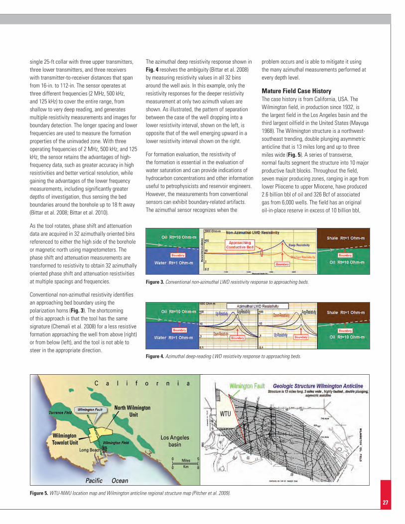
27

Figure 3. Conventional non-azimuthal LWD resistivity response to approaching beds.

Figure 4. Azimuthal deep-reading LWD resistivity response to approaching beds.

Figure 5. WTU-NWU location map and Wilmington anticline regional structure map (Pitcher et al. 2009).

single 25-ft collar with three upper transmitters, three lower transmitters, and three receivers with transmitter-to-receiver distances that span from 16-in. to 112-in. The sensor operates at three different frequencies (2 MHz, 500 kHz, and 125 kHz) to cover the entire range, from shallow to very deep reading, and generates multiple resistivity measurements and images for boundary detection. The longer spacing and lower frequencies are used to measure the formation properties of the uninvaded zone. With three operating frequencies of 2 MHz, 500 kHz, and 125 kHz, the sensor retains the advantages of high-frequency data, such as greater accuracy in high resistivities and better vertical resolution, while gaining the advantages of the lower frequency measurements, including significantly greater depths of investigation, thus sensing the bed boundaries around the borehole up to 18 ft away (Bittar et al. 2008; Bittar et al. 2010).

As the tool rotates, phase shift and attenuation data are acquired in 32 azimuthally oriented bins referenced to either the high side of the borehole or magnetic north using magnetometers. The phase shift and attenuation measurements are transformed to resistivity to obtain 32 azimuthally oriented phase shift and attenuation resistivities at multiple spacings and frequencies.

Conventional non-azimuthal resistivity identifies an approaching bed boundary using the polarization horns (Fig. 3). The shortcoming of this approach is that the tool has the same signature (Chemali et al. 2008) for a less resistive formation approaching the well from above (right) or from below (left), and the tool is not able to steer in the appropriate direction.

The azimuthal deep resistivity response shown in Fig. 4 resolves the ambiguity (Bittar et al. 2008) by measuring resistivity values in all 32 bins around the well axis. In this example, only the resistivity responses for the deeper resistivity measurement at only two azimuth values are shown. As illustrated, the pattern of separation between the case of the well dropping into a lower resistivity interval, shown on the left, is opposite that of the well emerging upward in a lower resistivity interval shown on the right.

For formation evaluation, the resistivity of the formation is essential in the evaluation of water saturation and can provide indications of hydrocarbon concentrations and other information useful to petrophysicists and reservoir engineers. However, the measurements from conventional sensors can exhibit boundary-related artifacts. The azimuthal sensor recognizes when the

problem occurs and is able to mitigate it using the many azimuthal measurements performed at every depth level.

Mature Field Case HistoryThe case history is from California, USA. The Wilmington field, in production since 1932, is the largest field in the Los Angeles basin and the third largest oilfield in the United States (Mayuga 1968). The Wilmington structure is a northwest-southeast trending, double plunging asymmetric anticline that is 13 miles long and up to three miles wide (Fig. 5). A series of transverse, normal faults segment the structure into 10 major productive fault blocks. Throughout the field, seven major producing zones, ranging in age from lower Pliocene to upper Miocene, have produced 2.6 billion bbl of oil and 326 Bcf of associated gas from 6,000 wells. The field has an original oil-in-place reserve in excess of 10 billion bbl,

28

AZIMUTHAL DEEP-READING RESISTIVITY FOR COMPLEX RESERVOIR EVALUATION

Figure 6. Pre-well proposed section (Pitcher et al. 2009).

Figure 7. Final drilled section (Pitcher et al. 2009).

with an estimated ultimate recovery of more than 3 billion bbl (Clarke and Henderson 1987).

The Wilmington productive section has a gross thickness of approximately 3,000 ft and comprises an aggradational succession of Miocene- and Pliocene-age confined slope deposits prograding into unconfined basinal-medial to distal-turbidite fan complexes. Medium- to thick-bedded hemipelagic mudstones separate successive lower-slope, medial, and distal-fan sand bodies. At the parasequence level, lithofacies comprise indurated mudstones, shales, and siltstones interbedded with semi-consolidated and unconsolidated fine- to coarse-grained sandstones.

The optimal positioning of a complex well in a thinly laminated reservoir that has already been produced required careful planning on the part of the asset team. The objective was to use a low angle trajectory to assess the potential for waterflooding in the lower zones of the reservoir that could negatively affect production. The goal was to determine the relative presence or absence of water before fully penetrating the lowest zone, which had the highest risk of waterflood. Fig. 6 shows the proposed plan in section.

After entry into the lower zone, the resistivity values from the bottom octant indicated that water was not present in this lower zone up to the detection limit of the tool. As the section was traversed, the measurement continued to indicate the absence of water, enabling the team to confidently drill the section (Fig. 7).

ConclusionsMaximum well contact and optimum well placement are key to increasing production from mature fields. Accessing and draining bypassed sweet spots in mature, thin, and complex fields to navigate reservoirs requires new directional deep-reading well placement technology. Azimuthal deep-reading resistivity tools provide real-time deep measurements necessary to detect bed boundaries and fluid contacts, to place the wellbore in the optimum position, and to maximize reservoir contact and production. Proper evaluation of the reservoir is also important in mature field development to minimize the uncertainties in reservoir characterization. Conventional LWD wave propagation resistivity

tools are influenced by bed boundary and anisotropy, making it very difficult to determine true formation resistivity necessary for petrophysical interpretation. Directional resistivity measurements offer a resistivity measurement that is free of boundary effects and accurate

anisotropy determination to yield accurate water saturations and better determination of oil in place. The case studies in this paper have shown how this technology can assist in the development and evaluation of mature fields.

29

References

Jason Pitcher is director of CamShale for Cameron based in Houston, Texas. He received his BS degree in geology from the University of Derby and his MS degree in mineral exploration from Imperial

College in London. Jason had 22 years of experience with Halliburton, having worked in multiple areas of data acquisition and interpretation. He developed and managed well placement operations around the world, contributing to multiple national and international geosteering campaigns. He has co-authored over 20 papers and articles on LWD tools, petrophysics, geosteering, and unconventional shale exploration and development. At Cameron, Jason is the director of CamShale looking to optimize surface systems in shale operations.

Michael Bittar is senior director of technology for Halliburton. He joined Halliburton in 1990 and since then has held various technical and leadership roles, including Halliburton technology fellow,

director of research, and senior director of formation evaluation. Michael received his BS, MS, and PhD degrees in electrical engineering from the University of Houston and has more than 100 patents and publications. Michael is a long-term member of SPE and SPWLA and was the recipient of the 2006 SPWLA Technical Achievement Award and the 2009 Halliburton Outstanding Commercialized Invention of the Year Award for his invention and development of azimuthal deep-reading technology.

Michael Dautel is the Asia Pacific technical advisor for Halliburton Sperry Drilling, based in Kuala Lumpur, Malaysia. He is responsible for LWD log interpretation, petrophysical support, and the

development of geosteering services. Michael has 28 years of experience in wireline and LWD operations and technology; he has worked in Australia, USA, Middle East, and Asia. Mike has an honors degree in electrical engineering and an MS degree in information technology from the Queensland University of Technology. He is a member of SPWLA and SPE.

Authors

Bittar, M. 2000. electromagnetic wave resistivity tool having a tilted antenna for determining the horizontal and vertical resistivities and relative dip angle in anisotropic earth formations. us Patent no. 6,163,155.

Bittar, M. 2002. electromagnetic wave resistivity tool having a tilted antenna for geosteering within a desired payzone. us Patent no. 6,476,609.

Bittar, M., Klein, J., Beste, R., hu, G., Wu, M., Pitcher, J., Golla, C., Althoff, G., sitka, V., Minosyan, V., and Paulk, P. 2007. A new Azimuthal Deep-Reading Resistivity Tool for Geosteering and Advanced Formation evaluation. Paper sPe 109971 presented at the sPe Annual Technical Conference and exhibition, Anaheim, California, usA, 11–14 november.

Bittar, M., Chemali, R., and Pitcher, J. 2010. Real-Time Proactive Optimal Well Placement using Geosignal and Deep Images. Paper OTC 20894 Offshore Technology Conference held in houston, Texas, usA, 3–6 May.

Bootle, R., Waugh, M., Bittar, M. et al. 2009. Laminated sand-shale Formation evaluation using Azimuthal LWD Resistivity. Paper sPe 123890 presented at the sPe Annual Technical Conference and exhibition, new Orleans, Louisiana, usA, 4–7 October.

Clarke, D.D. and henderson, C. eds. 1987. The stratigraphy of the Wilmington Oil Field. Geologic Field Guide to the Long Beach Area, Pacific section AAPG Guidebook, 57–68.

Mayuga, M.n. 1968. Geology and Development of California’s Giant – The Wilmington Oil Field, presented to the American Association of Petroleum Geologists, 53rd Annual Meeting, Oklahoma City, Oklahoma, usA, 22–25 April.

Pitcher, J., Bittar, M., hoyt, D., and henderson, J. 2009. Improving Recovery with Advanced Formation evaluation and Well Placement Techniques in Thinly Laminated sand-shale Reservoirs. Paper presented at the Offshore Mediterranean Conference and exhibition, Ravenna, Italy, 25–27 March.

Pitcher, J., Bittar, M., hinz, D., Knutson, C., and Cook, R. 2011. Interpreting Azimuthal Propagation Resistivity: A Paradigm shift. Paper sPe 143303 presented at the sPe euROPeC/eAGe Annual Conference and exhibition held in Vienna, Austria, 23–26 May.

Rodney, P., Mack, s., Bittar, M. et al. 1991. An MWD Multiple Depth of Investigation electromagnetic Wave Resistivity sensor. Paper D presented at the sPWLA 32nd Annual Logging symposium, Midland, Texas, usA, 16–19 June.

30

COST-EFFECTIVE ADVANCES IN SURVEY DESIGN ANALYSIS

Optimizing VSP Anisotropy Surveys with Reflection Data Ran Zhou, Bruce Cornish, Donghong Pei, and Dan Quinn, Halliburton

Presented at the SEG International Exposition and Annual Meeting, held in Houston, Texas, September 22-27, 2013. Copyright 2013, Society of Exploration Geophysicists, republished with permission.

SummaryAn analysis of walkaway and multi-offset VSP shows that reflection data in the multi-offset VSP can extend vertical-angle range covered by the direct arrivals and provide additional constraints to the estimated anisotropic parameters. Because raypaths in the reflection data are longer and different than the direct arrivals, using reflection data in conjunction with direct arrivals makes it possible to utilize multiple offset rather than walkaway VSPs in anisotropy estimation and, therefore, reduce acquisition costs. Tests with synthetic data show that anisotropic parameters for a layered model can be calculated from multi-offset VSP with resolution comparable to a walkaway VSP.

IntroductionCorrection for seismic anisotropy has become common practice in subsurface imaging and reservoir property estimation. A walkaway VSP offers the best dataset for the determination of anisotropy parameters, since the direct arrivals are usually well determined, and the depths are accurately known (Thomsen 2002). Fig. 1 illustrates a typical walkaway survey designed to measure average (or effective) anisotropic parameters, δ and ε, in the overburden. The survey deploys a 3-C geophone array at one depth in the borehole to record seismic data from a line of surface shot points. The average anisotropic parameters can be calculated from direct P-wave traveltime data, assuming that the overburden is transversely isotropic and the symmetry axis is vertical. The velocities in the symmetry axis are determined from a checkshot survey.

How good is the average anisotropy estimation from such a walkaway VSP compared to the true values? For the simplified anisotropy model in Fig. 1, the estimated average anisotropic parameters deviate from the true values of the surveyed layer by a large amount, as shown in Fig. 2. The effective parameters are 0.02 and 0.11 for δ and ε, as compared to 0.05 and 0.18 in layer #5 of the test model. Alternatively, if the walkaway VSP is surveyed over a larger or even the entire depth interval, a more detailed anisotropic depth profile can be determined from a travel-time inversion or local slowness analysis. Such a VSP survey, however, can be expensive.

It is important to provide an adequate depth profile of anisotropic parameters for seismic model building and make the survey cost effective as well. Because a VSP records both direct and reflected events, using reflection traveltime data in the calculation can further constrain the anisotropy estimation. Reflection events travel longer paths and have different raypath coverage than direct arrivals in a layer. These advantages may reduce the need for dense shot coverage in an anisotropy survey and therefore make it possible to substitute a multi-offset VSP for a walkaway VSP and still provide sufficient coverage.

In this paper, we use a synthetic dataset to examine angle coverage and traveltime sensitivity in walkaway and offset VSPs for the model in Fig. 1. We present a feasibility study to investigate the possibility of using multi- offset VSP to derive a depth profile of overburden anisotropy.

Angle Coverage and Traveltime Sensitivity Comparison – Direct versus Reflected ArrivalsWalkaway VSP. Angle coverage and traveltime sensitivity are key issues in survey design that affect the resolution of the anisotropic parameters. Fig. 3 shows the vertical incidence angles of the direct arrivals (red stars) for a receiver near the bottom of layer #5 (Fig.1) and the reflection angles (blue stars) at the bottom of the same layer for the reflected arrivals of a receiver near the layer top. For a ratio of maximum shot offset to the maximum receiver depth of around 1.5, the angle coverage is between 60° and 70°. Fig. 4 shows the traveltime sensitivity of layer #5 for the same direct and Figure 1. A 1-D layered anisotropy model and a sample anisotropy survey with a walkaway VSP. An array of 3-C

geophones is deployed in layer #5. For illustration only, one receiver is shown near the bottom of the layer.

Figure 2. Traveltime mismatch of best-fit effective anisotropy model (red stars) and data. The error in the estimated anisotropy is 0.03 for delta and 0.07 for epsilon. The blue stars show the mismatch of a constant anisotropy model based on a local anisotropy analysis.

31

Figure 6. Offset VSP angle coverage for layers #2 (a), #3 (b) and #5 (c). Red stars are incidence angles of direct P-wave arrivals for receivers inside the layer. Blue stars are reflection angles from the bottom of the layer for receivers inside and above it.

Figure 7. Traveltime differences of two sets of modeled values for direct and reflected arrivals of layer #5. The two models are the original anisotropic model with isotropic or anisotropic layer #5.

Figure 3. Walkaway VSP angle coverage for layer #5. Red stars illustrate incidence angles of direct P-wave arrivals for the receiver in Fig.1. Blue stars show reflection angles from the bottom of layer #5 for a receiver near the top of the same layer.

Figure 4. Walkaway traveltime sensitivity for layer #5. The curves show traveltime changes caused by a change of 0.01 in one anisotropic parameter while the other retains the original value (Figure 1).

Figure 5. Offset VSP shot and receiver locations. The model anisotropic parameters are the same as in Figure 1. Reflections from the bottom of layer #5 are displayed to show raypath coverage.

reflected arrivals, which varies between 0.5 and 1.5 ms for a change of 0.01 in the anisotropic parameters.

Comparing the two Figures, the reflected arrivals are more sensitive to the anisotropic parameters, even though the direct arrivals have a greater angular coverage. Mid- to long offsets seem to be sensitive to parameter delta. The low sensitivity in delta indicates a likely lower resolution in its estimated value. In addition, longer offsets are preferred to constrain the value of epsilon, as the sensitivity of epsilon increases with offset. Nevertheless, the angle range between 30° and 60°, which corresponds to the offset range between 4,000 ft and 8,000 ft, is important for both parameters for layer #5.

Offset VSP. To investigate if a multi-offset VSP may provide similar angle coverage and traveltime sensitivity as in the walkaway VSP, offset VSP shots are selected at 1,000 ft, 3,000 ft, 6,000 ft, and 9,000 ft, as shown in Fig. 5.

An array of receivers at 50 ft intervals covers the interval from 1,000 ft to 6,000 ft. The model parameters are the same as in Fig. 1.

Fig. 6 shows angular coverage of layer #2, #3 and #5, where the red stars indicate the incidence angles of the direct arrivals, and blue stars indicate reflection angles from the bottom of each layer, respectively. As the reflected arrivals fill in the gaps in the angle range of direct arrivals, combinations of the four offsets seem to provide good coverage for different layers in the test model. For the shallower layers, two or three offsets are sufficient (Figs. 6a and 6b). For layer #5, the two far offsets are important to offer good coverage (Fig. 6c).

Fig. 7 illustrates traveltime differences between the modeled values from the anisotropic model with isotropic and anisotropic layer #5, to offer an alternative view of traveltime sensitivity for different shot points. It is clear that larger offsets are more sensitive to the anisotropic effect owing to greater angular coverage and longer travel paths inside the layer. As a result, the large offsets are essential to constrain the anisotropic parameters for this deeper layer. Furthermore, the reflected arrivals recorded by the receivers inside and above the layer have longer traveltimes and, therefore, can provide better constraints on the anisotropic parameters.

Tests of Anisotropy Inversion with Multi-Offset VSPSeveral numerical tests were carried out to investigate the feasibility of using reflection traveltime data in conjunction with direct arrivals in a multi-offset VSP to recover the anisotropic parameters of the test model in Fig. 1. Synthetic

traveltime data were generated for the walkaway and offset VSPs using the layered anisotropy model. The inversion of the two anisotropic parameters was carried out iteratively using a generalized inversion method to monitor the improvement in estimated parameters,

32

COST-EFFECTIVE ADVANCES IN SURVEY DESIGN ANALYSIS

change in traveltime mismatch, and the resolution of the results. The vertical velocities of the model retained the original values during the inversion process.

Tables 1 through 3 summarize the results of three tests: (1) Inversion of layer #5 anisotropic parameters using three offset shots; (2) comparison of inversion results for layer #5 using offset and walkaway VSP; and (3) estimated anisotropic model using the multi-offset VSP.

Table 1 presents the inversion result for layer #5 (δ=0.05 and ε=0.18) using direct and reflected traveltime from three offset shots at 3,000 ft, 6,000 ft and 9,000 ft (Fig. 6c). This test investigates whether the anisotropic parameters can be resolved from the multi-offset VSP. The

direct arrivals of those receivers inside the layer and 200 ft below the upper layer boundary were used. The reflected arrivals of four receivers above the layer were also included, in addition to those inside the layer. The anisotropic parameters in other layers retained their original values during the inversion. The inversion process is fast and recovers the test parameters in the model quite well. At the end of the second iteration, the maximum error in the modeled traveltime is 0.6 ms, and the error in the estimated anisotropic parameter is -0.003 for δ and 0.005 for ε.

Table 2 compares the inversion results after the second iteration for layer #5 from three data sets: (1) walkaway direct arrivals, (2) offset direct arrivals, and (3) offset direct and reflected arrivals. The shot coverage of the walkaway

is shown in Fig. 1, and the direct arrival traveltime from one receiver near the bottom of layer #5 was used. The offset traveltime data were the same as in the first test. The offset shots in this noise-free case provide comparable results to the walkaway. Using the reflection data in conjunction with the direct arrivals produces better results for the estimated anisotropic parameters.

Table 3 shows the inversion result for the entire test model using both direct and reflected arrival traveltimes from the offset shots in Fig. 6. The inversion was carried out in a layer-stripping fashion. The first layer was assumed to be isotropic. For each layer, receivers inside that layer were used for direct and reflected arrivals. Four receivers above the layer were added to the reflection arrivals, as described in the first test. The shot selection for layers # 2 and #3 is shown in Fig. 6. For layer #4, the same shots for layer #3 were used. For layer #5, the three shots in the first two tests were used. As seen in the table the test model was recovered quite well from the inversion of the multi-offset VSP traveltime data. Although the errors in the estimated anisotropic parameters are similar, the relative errors in delta are higher than epsilon.

Discussion and ConclusionsThe example in this study shows that four offset shots provide a comparable angular coverage and traveltime sensitivity as compared to a walkaway for the test anisotropy survey. For a field survey, detailed pre-survey modeling is necessary to determine the shot offsets and the number of shots required. In the case where a walkaway VSP is surveyed for the depth interval around the target and a mid-offset VSP is designed for imaging, the offset VSP may be used to extend the anisotropy profile to shallow depths. In addition, since the inversion was carried out in a layer-stripping manner, the results illustrate the accumulation of errors in the estimated anisotropic parameters. A traveltime inversion that simultaneously addresses both direct and reflected traveltime datasets over the entire model can more effectively constrain the inversion results. Future research will be conducted to test the simultaneous inversion with a global optimization method (Pei et al, 2011).

Table 3 Inversion results for the test model from offset shots using both direct and reflected arrival traveltime.

Layer and iter.

(#)

estimated anisotropic parameters Traveltime errors (ms)

δ ε

Ori. est. error Ori. est. error Max RMs

2, 2 0.05 0.048 -0.002 0.10 0.101 0.001 0.1 0.1

3, 2 0.05 0.047 -0.003 0.15 0.152 0.002 0.3 0.1

4, 1 0.0 0.001 -0.001 0.0 0.001 -0.001 0.1 0.1

5, 3 0.05 0.053 0.003 0.18 0.178 0.002 0.4 0.1

Table 1 Inversion results from 3 offsets for layer #5 using both direct and reflected arrival traveltimes.

Iter#

Before inversion After inversion

Input values Traveltimeerrors (ms) Changes estimated values

δ ε Max RMs Δδ Δε δ ε

1 0.0 0.0 23.6 11.0 0.032 0.226 0.032 0.226

2 0.032 0.226 5.9 2.6 0.015 -0.041 0.047 0.185

3 0.047 0.185 0.6 0.2 0.003 -0.004 0.050 0.180

Table 2 Inversion results for layer #5 from offset and walkaway VsP.

Test dataestimated anisotropic parameters Traveltime errors (ms)

δ-est. error ε-est. error Max RMs

Walkaway (direct) 0.049 -0.001 0.187 0.007 0.9 0.4

Offsets (direct) 0.055 0.005 0.189 0.009 1.0 0.4

Offsets (direct + reflected) 0.047 -0.003 0.185 0.005 0.6 0.2

33

Acknowledgements

We are grateful to our colleagues at Halliburton who provided support for this research and improved the manuscript. We thank Halliburton for permission to publish this paper.

Ran Zhou of Halliburton Wireline and Perforating is the Manager of the Center for Advanced Borehole Seismic Solutions. Ran holds a PhD degree in geophysics from the University of Texas at Austin, and

has 20 years of experience in R & D in VSP processing technology, microseismic, and global geophysics. Her expertise includes advanced VSP processing, imaging, and interpretation; overburden seismic anisotropy estimation and depth imaging; shear-wave birefringence and fracture characterization; and seismic amplitude AVO analysis, modeling, and calibration.

Bruce Cornish is a Seismic Technical Advisor. He joined Halliburton through the acquisition of Geophysical Service Inc. in 1988, and holds BS and MS degrees in geology/geophysics from Southern Illinois

University. Bruce has broad experience in multicomponent borehole seismology, seismic while drilling, and micro seismology. He is a specialist in full-wave non-linear inversion and the integration of geologic, well log and seismic information for reservoir development, and is a long-term member of SEG and SPE.

Donghong Pei is currently a Senior Geophysical Advisor for Halliburton Energy Services in the Pinnacle microseimic monitoring group, focusing on seismic wave propagation, inversion, seismic

source mechanics, and petrophysics. Having been with Halliburton for seven years, Don holds a PhD in geophysics from the University of Nevada, Reno, and has published more than 20 abstracts and journal papers. He is a member of SEG.

Dan Quinn is the Borehole Seismic Global Strategic Business Manager, responsible for all aspects of Halliburton’s Borehole Seismic business. He holds a BSc in geology from Old Dominion University and

has 34 years of experience in the oil and gas industry with 30 years in Borehole Geophysics. Dan started his career with Western Geophysical, and has held various domestic and international positions. He is a published author, and holds a patent for a marine point source array design, with another patent pending. He is a member of SEG, EAGE, SPE, and AAPG.

References

Pei, D., B. Cornish, R. Zhou, D. Quinn, and R. Williamson, 2011, A VFsA Method of Travel Time Inversion for Layer Interval Anisotropy estimation using Walk-away VsP: eAGe workshop - Borehole Geophysics: emphasis on 3D VsP, Istanbul, Turkey, 16–19 January 2011

Thomsen, L., 2002. understanding seismic anisotropy in exploration and exploitation, seG/eAGe Dist. Instr. series no. 5, soc. expl. Geoph.

Authors

Although the tests show good results with noise-free data, it is important to be aware of the higher noise level in reflection arrivals as compared to direct arrivals. In addition, as the uncertainty of wavelet polarity in reflected data may add a systematic error in the traveltime,

the polarity of the reflection events needs to be verified before the inversion.

This study demonstrates that the reflection data in the VSP can extend or fill-in gaps in the vertical angle range covered by the direct arrivals. The

use of reflection data in conjunction with direct arrival traveltimes makes it possible to use just a few offset shots in providing a depth profile of overburden anisotropy. Further investigation will be carried out for field data tests and best practice survey designs. http://dx.doi.org/10.1190/segam2013-1324.1

http://dx.doi.org/10.1190/segam2013-1324.1

34

ENHANCED HYDROCARbON RECOVERY WITH MULTICOMPONENT INDUCTION TOOL

Evaluation of General Resistivity Density-Based Saturation in Thin, Laminated Sand-Shale Sequences John Quirein, Burkay Donderici, David Torres, Eric Murphy and Jim Witkowsky, Halliburton

Presented at the AAPG International Conference and Exhibition held in Singapore, September 16 – 19, 2012. Copyright 2012, reprinted by permission of the AAPG, whose permission is required for further use.

IntroductionThin, laminated sand-shale sequences can occur in all kinds of depositional environments, such as fluvial point bars, deltas, deepwater submarine fans, and turbidites and can trap significant amounts of hydrocarbons in the thin, sandy beds. Evaluation with conventional low-resolution uniaxial resistivity tools of the electrically anisotropic sand-shale sequences may result in significant underestimation of the hydrocarbon pore volume in the reservoir. A triaxial multicomponent induction tool can be used to characterize the electrical anisotropy in terms of the horizontal and vertical components of the formation resistivity. An interpretation model can be applied to convert the measured horizontal and vertical resistivities into the sand resistivity and sand volume. With the proper analysis, this translates into an enhanced hydrocarbon recovery and optimized reservoir development.

This paper provides a complete rock model and a comprehensive workflow that takes into account all the necessary stages to estimate water saturation in a thinly bedded sand-shale sequence, where both laminated and dispersed shale types can exist. It is shown that the Thomas-Stieber model can be applied, in conjunction with an approximation of total porosity, to compute the sand total and effective porosity. This allows net-pay cutoffs to be applied based on sand volume, porosity, and water saturation. Different clay-bound water sources will be assumed. If grain density information is available from sources, like downhole geochemical logging tools or wellsite energy-dispersive x-ray fluorescence, the process can be made more accurate by iteratively solving for porosity and saturation from the bulk density along with the horizontal and vertical resistivity measurements. This is accomplished by applying a robust and efficient nonlinear solver, which has been built to take into account the possible dependence of the fluid density on the saturation, as well as the dependence of the saturation and cementation exponents (N and M) on the total porosity.

Several field examples are presented for both wireline and LWD measurements. Dispersed shale is interpreted using any of the Dual-Water, Simandoux, and Indonesia equations.

Laminated Sand-Shale Sequences Interpretation ModelsThin laminated sand-shale sequences can occur in all kinds of depositional environments, such as fluvial point bars, deltas, deepwater submarine fans, and turbidites and can trap significant amounts of hydrocarbons in the thin, sandy beds. Resistivity anisotropy occurs from alternating thin beds or laminations of differing resistivity, where the individual bed thicknesses are less than the resolution of the resistivity tools (Klein 1993), and this kind of anisotropy is often called “macroscopic anisotropy.” In some stratified rocks, some grains possess a flat or elongated shape (e.g., mica and illite) and were laid down with an orientation parallel to the sedimentation strata at the time of deposition by nature and are often categorized as shale. Electric currents have a preferred path parallel to the bedding compared to perpendicular to the bedding, and this kind of anisotropy is referred to as “microscopic anisotropy” (Yin et al. 2008).

The paper by Yin et al. 2008 provides a good overview of many published resistivity anisotropy models prior to 2008. These models generally describe an effective resistivity anisotropy (macro anisotropy) resulting from the horizontal and vertical resistivities that are derived from tool measurements. Some of the models consider the intrinsic microscopic anisotropy of the shales. Note the industry convention is to use the notation, Rh, for the “horizontal” and Rv for the “vertical” resistivity, where, in reality, Rh is the derived resistivity parallel to the bedding, and Rv is the derived resistivity perpendicular to the bedding, as illustrated by Fig. 1 below.

A simple example is presented below to illustrate the effect of macro anisotropy on the horizontal and vertical resistivities derived from simulated tool measurements. In this simple example, we assume no dip and no shale micro anisotropy. In Fig. 2, the 1st track displays the physical model, where dark brown represents shale and tan represents sand. Track 2 shows that the upper

Figure 1. Illustration of the macro anisotropy concept.

Figure 2. Simulated data illustrating the effect of laminated beds and macro anisotropy on resistivities, Rh and Rv.

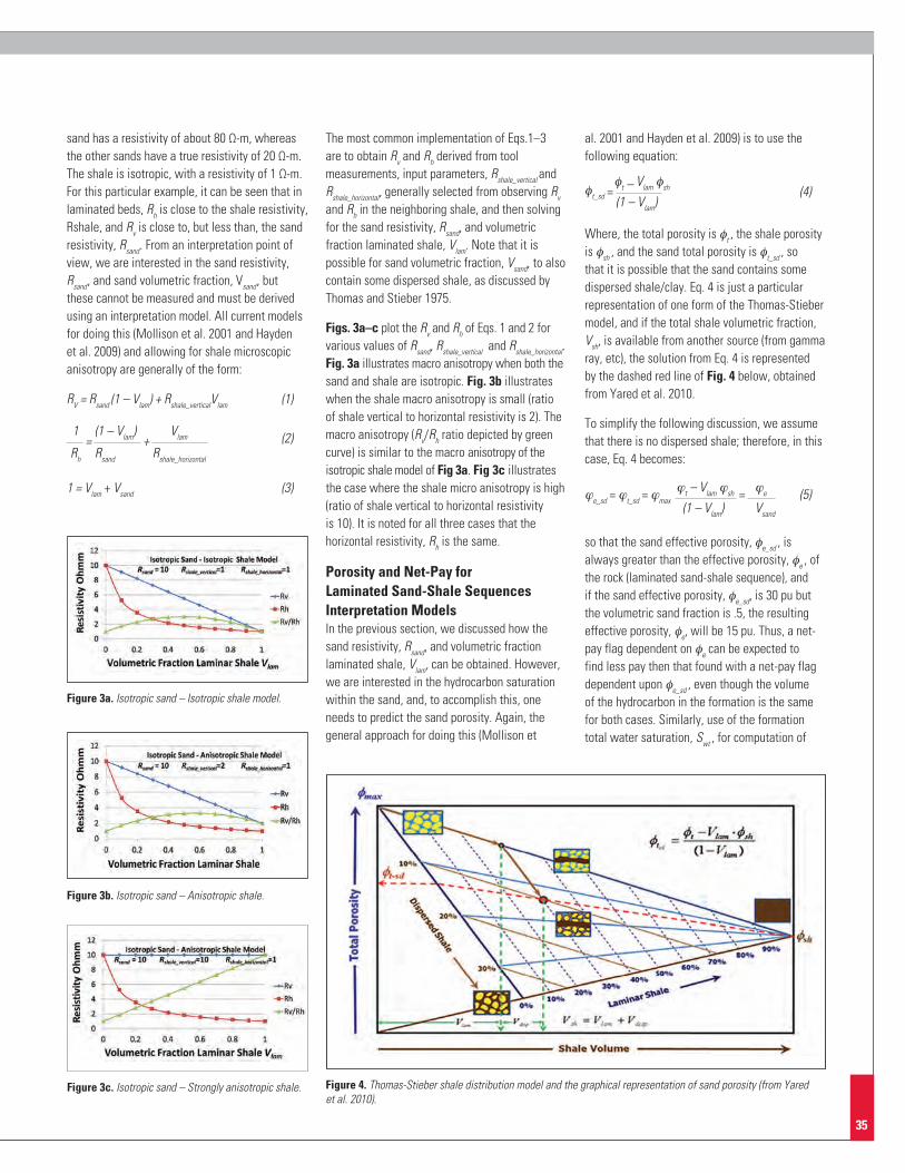
35

Figure 3a. Isotropic sand – Isotropic shale model.

Figure 3b. Isotropic sand – Anisotropic shale.

Figure 3c. Isotropic sand – Strongly anisotropic shale. Figure 4. Thomas-Stieber shale distribution model and the graphical representation of sand porosity (from Yared et al. 2010).

sand has a resistivity of about 80 Ω-m, whereas the other sands have a true resistivity of 20 Ω-m. The shale is isotropic, with a resistivity of 1 Ω-m. For this particular example, it can be seen that in laminated beds, Rh is close to the shale resistivity, Rshale, and Rv is close to, but less than, the sand resistivity, Rsand. From an interpretation point of view, we are interested in the sand resistivity, Rsand, and sand volumetric fraction, Vsand, but these cannot be measured and must be derived using an interpretation model. All current models for doing this (Mollison et al. 2001 and Hayden et al. 2009) and allowing for shale microscopic anisotropy are generally of the form:

RV = Rsand (1 – Vlam) + Rshale_verticalVlam (1)

1 (1 – Vlam) Vlam = + (2) Rh Rsand Rshale_horizontal

1 = Vlam + Vsand (3)

The most common implementation of Eqs.1–3 are to obtain Rv and Rh derived from tool measurements, input parameters, Rshale_vertical and Rshale_horizontal, generally selected from observing Rv and Rh in the neighboring shale, and then solving for the sand resistivity, Rsand, and volumetric fraction laminated shale, Vlam. Note that it is possible for sand volumetric fraction, Vsand, to also contain some dispersed shale, as discussed by Thomas and Stieber 1975.

Figs. 3a–c plot the Rv and Rh of Eqs. 1 and 2 for various values of Rsand, Rshale_vertical and Rshale_horizontal. Fig. 3a illustrates macro anisotropy when both the sand and shale are isotropic. Fig. 3b illustrates when the shale macro anisotropy is small (ratio of shale vertical to horizontal resistivity is 2). The macro anisotropy (Rv/Rh ratio depicted by green curve) is similar to the macro anisotropy of the isotropic shale model of Fig 3a. Fig 3c illustrates the case where the shale micro anisotropy is high (ratio of shale vertical to horizontal resistivity is 10). It is noted for all three cases that the horizontal resistivity, Rh is the same.

Porosity and Net-Pay for Laminated Sand-Shale Sequences Interpretation ModelsIn the previous section, we discussed how the sand resistivity, Rsand, and volumetric fraction laminated shale, Vlam, can be obtained. However, we are interested in the hydrocarbon saturation within the sand, and, to accomplish this, one needs to predict the sand porosity. Again, the general approach for doing this (Mollison et

al. 2001 and Hayden et al. 2009) is to use the following equation:

φt – Vlam φshφt_sd = (4) (1 – Vlam)

Where, the total porosity is φt , the shale porosity is φsh , and the sand total porosity is φt_sd , so that it is possible that the sand contains some dispersed shale/clay. Eq. 4 is just a particular representation of one form of the Thomas-Stieber model, and if the total shale volumetric fraction, Vsh, is available from another source (from gamma ray, etc), the solution from Eq. 4 is represented by the dashed red line of Fig. 4 below, obtained from Yared et al. 2010.

To simplify the following discussion, we assume that there is no dispersed shale; therefore, in this case, Eq. 4 becomes:

jt – Vlam jsh jeje_sd = jt_sd = jmax = (5) (1 – Vlam) Vsand

so that the sand effective porosity, φe_sd , is always greater than the effective porosity, φe , of the rock (laminated sand-shale sequence), and if the sand effective porosity, φe_sd, is 30 pu but the volumetric sand fraction is .5, the resulting effective porosity, φe, will be 15 pu. Thus, a net-pay flag dependent on φe can be expected to find less pay then that found with a net-pay flag dependent upon φe_sd , even though the volume of the hydrocarbon in the formation is the same for both cases. Similarly, use of the formation total water saturation, Swt , for computation of

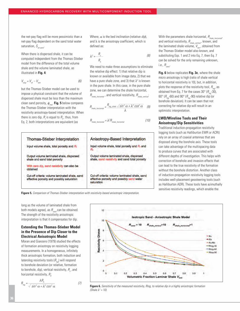
36

Figure 6. Sensitivity of the measured resistivity, Rlog, to relative dip in a highly anisotropic formation (Shale λ2 = 10).

Figure 5. Comparison of Thomas-Stieber interpretation with resistivity-based anisotropic interpretation.

the net-pay flag will be more pessimistic than a net-pay flag dependent on the sand total water saturation, Swt-sand .

When there is dispersed shale, it can be computed independent from the Thomas-Stieber model from the difference of the total volume shale and the volume laminated shale, as illustrated in Fig. 4:

Vdisp = Vsh – Vlam (6)

but the Thomas-Stieber model can be used to impose a physical constraint that the volume of dispersed shale must be less than the maximum clean sand porosity, φmax. Fig. 5 below compares the Thomas-Stieber interpretation with the resistivity anisotropy-based interpretation. When there is zero dip, Rt is equal to Rh ; thus, from Eq. 2, both interpretations are equivalent (as

long as the volume of laminated shale from both models agree), as Rsand can be obtained. The strength of the resistivity anisotropic interpretation is that it compensates for dip.

Extending the Thomas-Stieber Model in the Presence of Dip Closer to the Electrical Anisotropic ModelMoran and Gianzero (1979) studied the effects of formation anisotropy on resistivity logging measurements. In a homogeneous, infinitely thick anisotropic formation, both induction and laterolog resistivity tools (Rlog) will respond to borehole deviation (or relative, formation to borehole, dip), vertical resistivity, Rv , and horizontal resistivity, Rh:

Where, α is the bed inclination (relative dip), and λ is the anisotropy coefficient, which is defined as:

Rv l2 = (8) Rh

We need to make three assumptions to eliminate the relative dip effect: 1) that relative dip is known or available from image data, 2) that we have a pure shale zone, and 3) that λ2 is known in the pure shale. In this case, in the pure shale zone, we can determine the shale horizontal, Rshale_horizontal , and vertical resistivity, Rshale_vertical:

(9)

Rshale_horizontal = l2Rshale_horizontal (10)

With the parameters shale horizontal, Rshale_horizontal, and vertical resistivity, Rshale_vertical , known, and the laminated shale volume, Vlam , obtained from the Thomas-Stieber model also known, and substituting Eqs. 1 and 2 into Eq, 7, then Eq. 7 can be solved for the only remaining unknown, i.e., Rsand .

Fig. 6 below replicates Fig. 3c, where the shale micro anisotropy is high (ratio of shale vertical to horizontal resistivity is 10), but, in addition, plots the response of the resistivity tool, Rlog, as obtained from Eq. 7 for the cases 30° (Rlog-30), 60° (Rlog-60) and 90° (Rlog-90) relative dip (or borehole deviation). It can be seen that not correcting for relative dip will result in an optimistic interpretation.

LWD/Wireline Tools and Their Anisotropy/Dip SensitivitiesTraditional induction-propagation resistivity logging tools (such as Halliburton EWR or ACRt) rely on an array of coaxial antennas that are disposed along the borehole axis. These tools can take advantage of the multispacing data to produce curves that are associated with different depths of investigation. This helps with correction of borehole and invasion effects that can lead to the true resistivity of the formation without the borehole distortion. Another class of induction-propagation resistivity logging tools includes well-placement geosteering tools (such as Halliburton ADR). These tools have azimuthally sensitive resistivity readings, which enable the


37

determination of position and orientation of boundaries around the wellbore. Both logging and well placement tools are used to evaluate anisotropy of formations; however, they have a limitation on the minimum dip angle that they can operate with for reliable operation (determination of Rv, Rh, and dip) owing to the low sensitivity of the signal components used in these tools at low dip angles. Multicomponent induction tools (such as Halliburton Xaminer™ MCI) are developed to reliably measure anisotropy of formations. These tools feature nine tensor components composed of three transmitter orientations and three receiver orientations. Fig. 7 below shows the signal components that are available in each type of tool and the percentage sensitivity of each component to Rv and dip as a function of dip angle. The sensitivity displayed is the sensitivity of a component divided by the sum of all components where sensitivity is defined as the change on the signal due to change in the parameter (anisotropy constant in this case).

As shown in Fig. 7, traditional resistivity tools only have the ZZ component, which is sensitive to anisotropy only if the dip is larger than 70° (see the right-hand plot in Fig. 7). Geosteering tools have XZ, YZ, ZX, and ZY in addition to the ZZ component, which widen the reliable anisotropy inversion range to dip above 40°. Anisotropy tools, on the other hand, are sensitive to all nine components, including XX and YY, which are maximally sensitive to anisotropy and dip around zero dip angle. As a result, anisotropy tools can reliably measure anisotropy and intrinsic dip of formations at any dip angle.

Wireline Anisotropy Tool: Xaminer™ MCI The Xaminer™ MCI (Fig. 8) has a transmitter triad (collocated triaxial array of 3 coils) and 6 sets of receiver coils. The 2 closest receiver coils to the transmitter are standard induction coils, while the remaining 4 coils are built as triads. The tool operates by sequentially energizing each of the coils (X,Y,Z) in the transmitter triad and measuring the signals in each of the receiver coils. Hence each of the receiver triads produce 9 signals per frequency. These signals are corrected for borehole effects and then inverted to obtain the desired formation measurements. Rh, Rv, Relative (formation to borehole) Dip and Azimuth. Usually the tool is run with a directional package so that true formation Dip and Azimuth can be found and is also run with a 6-arm caliper to find the relative position of the tool in the borehole.

Figure 9. Diagram of a multitriad triaxial induction array showing configuration and its equivalent dipole model (for one triad) in the tool/measurement coordinate system (xt, yt, zt). Lm is the spacing between transmitter and main receiver coils (from Hou et al. 2012).

Figure 8. Configuration of Halliburton’s Xaminer™ MCI tool.

Figure 7. Different resistivity tool types and sensitivity to anisotropy and intrinsic dip.

The tool also provides the same logs as the Halliburton ACRt tool. To do this, the transmitter spacings are the same as the ACRt tool and, like the ACRt, it also uses 3 frequencies to do the Skin Effect correction. All the signals measured on the Z receivers when the transmitter is fired follow the same processing as the standard ACRt tool to match the response of the ACRt tool.

The tool operates centralized in boreholes filled with air or oil-based muds. Each receiver triad is an arrangement of 6 coils: 3 main and 3 bucking coils, each pair for one of the 3 orthogonal directions X,Y,Z and is represented diagrammatically with its equivalent dipole

model in Fig. 9. Both the main and bucking coils are collocated, and the bucking coils are wound as to minimize the direct coupling signals. The transmitter triad only has 3 main collocated coils. Each triad sends up hole a 9-component complex tensor for each frequency. The tool energizes the formation with 4 frequencies simultaneously. All of the information from the 4 triads, plus the short spacing information, is converted into a digital string that is sent uphole via the telemetry system. All of these voltages are calibrated to mmh/m, and all of the signals are compensated for temperature changes in the sonde error, electronics drifts, and changes in gain. The uphole processing software calculates

38

Figure 10. Graphical representation of the solutions to Eqs. 1–3 for Rshale_vertical = 10 and Rshale_horizontal = 1 (From Minh et al 2008).

Figure 11. Anisotropic model interpreted results from the Fort Worth, Texas, test well.

the tool position in the borehole and removes any effects from tool position and borehole effects. To do so, a first 1-D radial inversion algorithm is used. As a result of this inversion, a first quick look of the results (Rh, Rv, dip, azimuth) can be presented in real time, and all of the borehole corrected tensors can be presented. The borehole corrected tensors are the input (post real time) to a 1-D vertical inversion algorithm. This algorithm squares the log, and the results give answers that have reduced shoulder bed effects. All the details are provided by Hou et al. 2012.

Field Log Fort Worth, Texas, Test Well Example Wireline Anisotropy Tool: Xaminer™ MCI A prototype of the new tool was well tested in Fort Worth, Texas, and an anisotropic interpretation was performed using Eqs. 1–3 to estimate the sand resistivity and volume–laminated shale. The data in this formation is basically a sequence of sands and shales, but the shale has a lot of micro-anisotropy and was modeled from observation of the data with shale horizontal, Rshale_horizontal = 6 Ω-m, and vertical resistivity, Rshale_vertical = 70 Ω-m. Note that the interpreted results are very sensitive to these parameters when there is a lot of laminated shale, as illustrated by Fig. 10 below from Minh et al. 2008. In this figure, the red contours correspond to values of constant sand resistivity. Note that they all converge to a common “pure shale point”. Actual data lying within the black circle will exhibit a lot of variability in the computed value for the sand resistivity, Rsand.

The blue contours represent values of constant laminated shale volume, Vlam. Note that resolution becomes degraded for values of Vlam greater than 0.5.

Fig. 11 below presents the anisotropic interpretation of the test well MCI data. Track 1 represents the resistivity. Because there is zero relative dip, the horizontal resistivity, as shown in blue, overlays the deep induction resistivity, as shown in red. The light blue cyan curve is the vertical resistivity and the orange curve is the interpreted sand resistivity. Track 2 represents the lithology, dark green representing clay, light green silt and yellow sandstone. In this track, the dispersed shale-bound water is orange, the laminated shale-bound water is light blue, and the free water is dark blue. Track 3 represents the neutron and density porosity logs. Track 4 represents the volume of laminated shale (green) from the MCI anisotropic interpretation and the volume of dispersed shale (purple) computed from the difference of a shale volume computed from a gamma ray minus the volume laminated shale. Note here that the volume of dispersed shale is inconsistent with the Thomas-Stieber model, which states that the maximum dispersed shale must be less than the shale porosity (about 6 pu). Thus, there is an inconsistency between the externally supplied shale volume, MCI-computed laminated shale volume, and the Thomas-Stieber model, which need to be resolved but will not be here because of a lack of geological data. Note that below approximately 1,800 ft, where there is a lot of laminated shale, the sand resistivity

becomes noisy for data in the vicinity of the pure shale point as discussed earlier.

Additional LWD and Wireline Field ExamplesThese examples will be presented at the AAPG Singapore conference subject to acquiring data release forms from the operators.

ConclusionsThis paper provided a complete rock model and a comprehensive workflow that takes into account all the necessary stages to estimate water saturation in a thinly bedded sand-shale sequence, where both laminated and dispersed shale types can exist and anisotropic resistivity data is available.

A comparison between the Thomas-Stieber model and the anisotropic resistivity model has been made. It has been shown that these models can be equivalent when there is no relative dip. When there is dip, both models can be equivalent if: 1) that relative dip is known or available from image data, 2) that we have a pure shale zone, and 3) that the anisotropy coefficient, l2, is known in the pure shale.

A net-pay flag dependent on formation effective porosity, φe , can be expected to find less pay (cumulative footage) then that found with a net-pay flag dependent on sand effective porosity, φe-sd , even though the volume of the hydrocarbon in the formation is the same for both cases.


39

Charts have been constructed showing how the MCI horizontal, Rh, vertical, Rv, and deep induction, Rlog, resitivities vary as a function of laminated shale volume and dip.

Wireline/LWD tools sensitivities to dip and anisotropy have been presented. It has been shown that “geosteering tools” can be used

for an anisotropic interpretation as long as the relative dip is greater than 40°. The newer LWD and wireline anisotropic tools are suitable for anisotropy interpretation at any relative dip.

The basic acquisition, processing and interpretation principles of a new wireline anisotropic tool have been summarized.

An example from a test well has been presented demonstrating the sensitivity of the anisotropic resistivity model to the input parameters. The model is particularly sensitive to minor data perturbations in the vicinity of the “pure shale point”.



Burkay Donderici is the Electromagnetics Manager at Halliburton. He received his PhD in electrical and computer engineering from Ohio State University, and has been with Halliburton for six years,

working in the electromagnetics and acoustics groups. He has been leading the Electromagnetics Sensor Physics team for Halliburton since 2011, and is currently involved with research and development of technologies, based on electromagnetics for oilfield applications.

David Torres is the Project Manager for the XaminerTM MCI tool, and is responsible for overseeing the development, testing, and marketing of the tool. For more than 20 years, David has worked in various

management and R&D positions. He began his career in 1980 with Gearhart Industries in Brazil, then moved to Texas and held several positions within Halliburton. He holds several patents and has authored various papers in signal and image processing. David holds an EE degree and an MSEE degree from the University of Madison, Wisconsin.

Eric Murphy was a log analyst for Halliburton in the Formation and Reservoir Solutions group. He joined Western Atlas Logging Services as a field engineer in 1994 after earning a BS in electrical engineering from the

University of Missouri - Rolla. Eric has also held global technical advisor positions at Baker Atlas, specializing in NMR and wireline formation testing and sampling. In 2013 Eric joined Chesapeake Energy in Oklahoma City as a Sr. Petrophysicist. He is a member of SPE and SPWLA.

Jim Witkowsky is the Technical Advisor for Halliburton’s Petrophysics Technology Development Group working with GEM elementals and mineral analysis in Shale Plays. He graduated

from the University of Pittsburgh with a degree in chemical/petroleum engineering, and began his career in 1986 as a general field engineer for Schlumberger, working primarily in the Gulf of Mexico. He was with the NUMAR Corporation in 1992 to 1997, where he held various positions, including NMR field engineer for the US, Indonesia, and Australia; manager of Australia field operations, and petrophysicist. Following the NUMAR merger with Halliburton, Jim was assigned to the Halliburton Formation and Reservoir Solutions (FRS) center as an NMR petrophysicist, responsible for client products, interpretations, and NMR Training. He is a member of SPWLA and SPE.

Authors

References

hayden, R., Kosten, A., Jacobson, s., Grant, J., Alderman, s., Katon, B.’ Liu, C.B., schwartz, K., Pham, T. 2009. Thin Bed Interpretation Techniques for northwestern Gulf of Mexico Coastal and Offshore Clastics. houston 2009 sPWLA Annual symposium.

hou, J, san Martin, L., Wu, D., Celepcikay, F.T., and Torres, D. 2012. Real-Time Borehole Correction for a new Multi-Component Array Induction Logging Tool in OBM Wells. Paper presented at the sPWLA 53rd Annual Logging symposium, Cartegena, Colombia, 16–20 June.

Klein, J.D., Martin, P.R., and Allen, D.F. 1997. The Petrophysics of electrically Anisotropic Reservoirs. Paper hh presented at the 1995 sPWLA Annual Logging symposium.

Minh, C.C., Clavaud, J., sundararaman, P., Froment, s., Caroli, e., Billon, O., Davis, G., and Fairbairn, R. 2008. Graphical Analysis of Laminated sand-shale Formations in the Presence of Anisotropic shales. Petophysics, 49(5): 395–405.

Mollison, R.A., Fannini, O.n., Kriegshauser, L., Yu, L., ugueto, G., and van Popta, J. 2001. Impact of Multi-component Induction Technology on a Deepwater Turbidite sand hydrocarbon saturation evaluation. Paper presented at the houston 2001 sPWLA Annual Logging symposium.

Moran, J.h. and Gianzero, s., 1979, “effects of Formation Anisotropy on Resistivity-Logging Measurements,” Geophysics, vol. 44, no. 7, July 1979, p. 1266-1286.

Thomas, e. and stieber, s. 1975. The Distribution of shale in sandstones and its effect upon Porosity. Paper presented at the 16th sPWLA Annual Logging symposium.

Yared, K., Pelorosso, M.,Altintutar, I., Buster, D., Manuel, e., Doyle, J., and Russell, C. 2010. novel Approach to Quantifying Deepwater Laminated sequences using Integrated evaluation of LWD Real-Time shear, Porosity, Azimuthal Density and high-Resolution Propagation Resistivity. Paper sPe 134515 presented at the Deepwater Drilling and Completion Conference, Galveston, Texas, usA, 5–8 October.

Yin, Y. and Kurniawan, B. 2008. Resistivity Anisotropy Models and Multi-Component Induction Measurements: Impact on sw and uncertainty of PPV estimation. Paper LLLL presented at the 2008 sPWLA Annual symposium.

40

Investigating the Dynamic Three-Dimensional Loading Effects on Perforating Guns Imposed by Shaped ChargesG.G. Craddock, Wei Zhang, and Jim Wight, Halliburton; John Rodgers, Timothy S. Glenn, Marco Serra, and Thomas Bettenmann, Starboard Innovations, LLC

This paper was prepared for presentation at the International Petroleum Technology Conference held in Doha, Qatar, 20–22 January 2014. Copyright 2014, International Petroleum Technology Conference

AbstractModern developments in shaped charge technology have resulted in greater explosive loads being used on perforating guns, which has stretched the capacity of perforating guns into uncharted territory. Traditional gun design approaches and standards use collapse pressure calculation and swell measurement with overloaded charges as design verification methods. The extremely complicated interactions between explosives, fragmented casings, and the gun wall are evaluated on an empirical basis, and the nature of these interactions is not well understood. In this paper, a new design model is presented that augments traditional design approaches and provides gun designers with better data on gun system structural performance, including the effects of phasing, shot density, and charge type.

The loads imposed on the gun body by the explosives are multidimensional because of the spiral arrangement of most shaped charges. The resulting dynamic response of the gun body is therefore quite complex and requires three-dimensional (3D) analysis. High-frequency bending, torsion, and tensile loads are expected. The casings are typically fragmented, and some of the larger fragments can impose high-impact loads on the gun wall. A fully coupled computer model has been developed that incorporates the rapid explosion, casing fragmentation, and multidimensional structural responses.

Multiple instrumented surface tests were performed to validate the dynamic 3D model. Proprietary testing techniques were used to extract gun internal pressure history and gun stress history at multiple locations immediately following detonation. Redundant strain gauges were used, and shots were repeated to ensure the integrity of the data.

This paper presents the instrumented gun test setup and results, along with the newly developed 3D simulation model and shock hydro model results. This paper also presents validation of the newly developed 3D model through comparisons with test data.

IntroductionCritical to the understanding of perforating gun/charge dynamics is the undertaking of instrumented gun testing in a controlled environment. Accurate downhole data collection within the perforating string has historically been challenging or impossible within close proximity to the charges. Previous attempts have produced limited results, with indirect fluid communication between charges and the transducer (Schatz et al. 2004). Surface testing using instrumentation to capture fluid pressures and structural response can provide valuable input for the design of more robust gun systems. Unfortunately, it is difficult to locate sensors in close proximity to an explosive event and to have them survive and produce quality data (Han et al. 2010). New tools and testing methods are required to perform such measurements.

In this paper, a sensor sub solution is presented for accurately measuring the shock response of a detonating gun. This tool is used to characterize an array of charges and gun systems. The data are then used to calibrate a proprietary finite element analysis (FEA) -based software package developed

for simulating the perforating event. A shock hydrodynamics code (CTH) is then used to better understand the dynamics of guns near the scallop. Three configurations are presented, with test data and comparisons to simulations: 1) a small-diameter gun with four small charges, 2) a small-diameter gun with a full charge load, and 3) a large-diameter gun with four large charges. The discussion concludes with lessons learned about charge-gun dynamics. Section I is the introduction, Section II is the surface test setup, Section III is the presentation of the test data and comparison to the FEA simulation, Section IV is the shock hydro simulation results, and Section V is the discussion and conclusions.

Test SetupTesting was performed in the test pond at Halliburton’s Jet Research Center (JRC) in Alvarado, Texas. The test tool consisted of a 2-ft gun loaded with a desired number of charges mated directly to a sensor sub (Figs. 1 and 2). The sensor sub includes a

dynamic pressure transducer exposed directly to the gun internal volume. A blast shield located in front of the sensor protects it from shrapnel while allowing ample fluid communication to the sensor face. Proper sensor integration is critical for avoiding pitfalls of introducing undesirable measurement dynamics or noise (Walter 2004; Dibbern et al. 2009). The sensor sub also includes axially oriented strain gauges (120° array) for

SHAPED CHARGE LOADING EFFECTS ON GUNS

Figure 1. 4 5/8-in. test tool suspended over test pond at Halliburton JRC.

41

measuring structural waves from the detonation. On the opposite end, the loaded gun is closed off with a crossover to a 3 3/8-in. blast sleeve housing a RED® detonator. Sensor subs are either 4 5/8- or 6 1/2-in. diameter, depending on the size of the charge being tested. The test string configurations are shown in the drawings in Fig. 2. The three configurations presented in this paper are described in Table 1.

For each test, the test string was supported vertically and submerged in a pond (Fig. 1). Data were recorded through an umbilical to a high-speed data acquisition system. The bandwidth of the pressure transducer and signal conditioner was >180 kHz, while the strain gauges and conditioners were >110 kHz. After each test, the blast shield was removed, and the face of the transducer was inspected and prepared for the next test.

Test and Software Simulation ResultsIn this section, results are presented for the three test configurations, along with comparisons to simulations using software. The FEA-based software package was developed to simulate the shock response of the bottomhole assembly (BHA) and wellbore to gun detonation. The model was calibrated using the surface test data, and a consistent set of calibration parameters were set for each charge type/gun system. Calibration parameters included gun remnant, which was used to quantify the partition of energy from the initial detonation (Grove et al. 2006), as well as damping. The data presented herein represent a subset of the surface tests run for this purpose.

Results for the Configuration 1 test and model are presented in Figs. 3 and 4. The model accurately tracked the physical behavior of the pressure waves within the gun, as well as the structural waves that propagated into the sensor sub. Some initial high-frequency dynamics in the first 0.5 microseconds of the fluid simulation are not observed in the data. However, the pressure impulse (integrated pressure history) shown in Fig. 5 can be used (Han et al. 2010) to illustrate how closely the simulation matches the data in overall energy. Some high-frequency dynamics apparent in the first 0.5 to 1 microsecond of the data are the result of shock-induced, acceleration sensitivity of the pressure transducer and data cables.

Observations from the FEA-based software package provide a better understanding of the

Figure 3. Plots of pressure and strain for three repeat shots of four 47-g BH/LD charges (Configuration 3): (left) pressure and (right) strain.

Figure 2. Drawing of test assembly for three configurations: 1, 2, and 3 (from top to bottom).

Table 1 - Test Configurations

Configuration Charge Type* Charge Count Gun Size (in.) Shot Density (spf)

1 22.7 g DP 4 4 5/8 12

2 22.7 g BH/LD 13 (Full load) 4 5/8 12

3 47 g BH/LD 6 1/2 114

DOI based on RT 100 Ohm-m and thickness of 30 ft

Figure 4. Comparison of test data and FEA model for four 22.7-g DP charges (Configuration 1): (left) pressure and (right) strain.

Pressure transducer assembly

Blast shield

42

Figure 8. 3D CTH simulation of 22.7-g DP charge in free space.

Figure 9. 3D CTH simulation of a single 22.7-g charge in a gun.

Figure 5. Comparison of test data and FEA model for pressure impulse with four 22.7-g DP charges (Configuration 1).

Figure 6. Comparison of test data and FEA-based software package for a fully loaded 22.7-g BH/LD gun (Configuration 2): (left) pressure and (right) strain.

Figure 7. Comparison of test data and FEA model for four 47-g BH/LD charges (Configuration 3): (left) pressure and (right) strain.

timing of the waves that were generating the observed pressure behavior. The initial large peak correlates in time with the pressure wave from the nearest charge reaching the transducer location. Lesser peaks correlate with pressure wave reflections off the ends of the gun interior volume.

Results from the Configuration 2 test data and model for a fully loaded gun are shown in Fig. 6. Compared to the previous case, responses are higher in amplitude. Some high-frequency noise is more apparent in the strain data with the greater charge load. The matching of the pressure and strain is also quite good for this case. Pressure dynamics after the initial peak are smoothed with the greater charge load.

Finally, Configuration 3 results for a larger charge and gun system are shown in Fig. 7. Note the good comparison to internal pressure data and strain at the sensor tool.

Shock Hydro SimulationsThe previous section used an FEA code to compare to test data. This constructed simulation does not model detailed charge dynamics, including details near the scallop. These details provide insight and hard numbers that can be used to augment the FEA simulation. Shock hydro simulations were setup using CTH (Crawford 2010) to examine these ignored areas. CTH is a

high-fidelity shock hydrodynamic code developed by Sandia Labs, which uses Eulerian methods. Simulations were performed with the 22.7-g DP charge and the 47-g BH charge. In the latter case, both a bare charge and a charge in a gun are presented. In the former case, a charge with the section of the gun with the scallop is presented. First, the 22.7-g charge was simulated. Fig. 8 shows the 3D simulations of the bare charge. Note that the jet is thin and the charge has a sharp apex angle. The purpose of this charge is to punch deep into the formation. Fig. 9 shows how this charge resides in a slick-wall gun and the penetrations into the gun. Equilibration time is roughly 68 microseconds, indicating a transition from 3D to two-dimensional (2D) gas/fluid behavior inside the gun. The hole size was similar to those in the tests. Pressures were measured at the transducer location in this somewhat under-resolved 3D simulation, but were lower than tested levels. Further work is required.

One set of simulations examined the immediate scallop area for a 47-g BH charge. This charge


43

Figure 11. Slices of the 3D CTH simulation in two symmetry directions. Note that the isotropic pressures are similar, with the transverse slice having a slightly larger value.

Figure 12. 3D CTH run slices with different materials inside and outside the gun. Air is inside the gun, while water is outside.

Fig. 10. 3D CTH simulation of a 47-g charge with a scallop plate. Note that the jet is purposely large at the tip to punch a larger hole in the casing plate.

is more relevant for deepwater Gulf application. Simulations were constructed in 2D initially, and the isotropic pressure to the scallop was calculated two ways: on a flat scallop and a curved scallop. In Fig. 10, a 47-g charge is shot through a 6 1/2-in. gun at 37.6 microseconds after detonation. Note that, as is typical of BH charges, the jet has a tendency to particulate. The charge casing is zinc and shows the tendency to break up. The zinc was modeled with a Mie-Gruniesen EOS and a Von Mises yield surface mode for strength with the CTH single value fracture model. Fig. 11 shows slices at 90 microseconds in the two symmetry directions around the scallop. The one-dimensional (1D) plots are of the isotropic pressure in the scallop material 90° apart.

These data augment the FEA model for gun survivability by providing realistic pressure numbers to input into a fracture model.

In the next set of simulations, the dynamics around the scallop were examined. The second setup was in three dimensions, and the charge was a 47-g BH charge in a 6 3/4-in. gun. In Fig. 12, the materials near the scallop are compared. Note that the jet characteristics change with the materials around the scallop and the gun hole size. An interesting aspect of the previous study is that a vacuum was used for the gas and water fill. By adding the water outside the gun and air inside the gun, the measured (computational) pressures near the

scallop in the gun change. Specifically, inside the scallop, pressure increases for higher-density (and pressure) fluid on the outside of the scallop and decreases for higher pressure on the inside of the gun. Fig. 13 shows the locations where pressures were recorded. Figs. 14 and 15 display the results. Note that these results indicate that

the high pressures near scallops generated by charges are dependent on the material butting up against the gun.

Finally, 2D and 3D simulations were run that more carefully examined the impact of the casing on the gun. Clearly, as shown in Fig. 16,

44

Figure 13. Locations of tracers, or points where the pressure is dumped in the 3D simulation.

Figure 14. Pressure tracers at two locations referenced in Figure 13.

Figure 15. Pressure plots at two tracer locations for room air temperature and 5,000-psi air.

Figure 16. Johnson-Cook (1985) damage on the inside of a gun in 2D. Note the areas of damage at 30° from vertical caused by charge casing.

Figure 17. A scallop hole inside the gun. Note the indentations from the casing.

the case in 2D caused damage to the gun when using the 47-g charge away from the scallop. Johnson and Cook (1985) note that a value of 1-in. damage means it has yielded or failed. The damaged regions roughly 30° from vertical were caused by the casing moving upward into the gun. In the 3D simulations, a similar behavior was observed. Moon-/semicircular-shaped pock marks were visible on the interior of the gun of the casing (Fig. 17). Note that a damaged region now exists for the charge around a scallop and in the region where the casing interacts with the gun. These two stress concentrations are then more likely to connect, as well as somewhat more distant additional charge casing pock marks. This interesting pattern is observed in surface fire guns. By mitigating the moon-/semicircular-shaped region through material or work hardening, the potential effect of the casing on a gun can be mitigated.

Discussion and ConclusionThis work presents surface test data and simulations combined to better understand gun longevity. The test data provided input for simulations to measures a gun’s nearness to failure. The testing consisted of two aspects: surface and downhole. This paper discusses the surface testing, while a later paper will discuss the downhole testing and simulation results.

Two types of simulations were used in this study. First, an FEA-based software package was shown to be a reasonable match to the test data. Yet, this package does not provide detailed charge dynamics, including effects around the immediate

area of the scallop. This code was used to compare to the test data. The second code, CTH (Crawford 2010), was used to examine the region around the scallop. Information gathered here provided input to the less resolved FEA simulation. Such high-fidelity local simulations provide additional information that the FEA simulations cannot. Thus, this study provides a method for increasing gun longevity by using surface test data to benchmark global simulations and high-fidelity shock hydro simulations to examine the local details.

The principal results of this paper are the following:• A new testing sub and test methodology have

been developed to improve gun system design and simulation accuracy. The results show excellent repeatability for both pressure and strain measurements.

• Surface tests provide calibration for specific gun-charge systems. FEA simulations using consistent calibration for each gun system have shown good correlation with data.

• High-fidelity shock hydro calculations indicate large pressures in the vicinity of the scallop. These pressures depend on the material both inside and outside the gun wall.

This paper focuses on surface test data. In a companion paper to be presented later, downhole data from a shock sensing sub will be presented and compared to the FEA simulation. This sub has the capability of measuring strain, acceleration, wellbore pressure, and temperature.


45

References

Crawford, D.A. 2010. CTh user’s Manual and Input Instructions. Albuquerque, nM: sandia national Labs.

Dibbern, A., sipes, W., hagopian, M. et al. 2009. Implications of Dynamic Pressure Transducer Mounting Variations on Measurements in Pyrotechnic Test Apparatus. Paper presented at the 45th AIAA/AsMe/sAe/Asee Joint Propulsion Conference & exhibit, Denver, Colorado, usA, 2–5 August.

Grove, B., Werner, A., and han, C. 2006. explosion-induced Damage to Oilwell Perforating Gun Carriers. structures under shock and Impact IX. WIT Transactions on The Built Environment 87: 165–175.

han, C., Du, M., and Ference, B. 2010. effect of shaped Charge Case Materials on Perforating Guns. Paper sPe 130477 presented at the CPs/sPe International Oil & Gas Conference and exhibition, Beijing. China, 8–10 June. http://dx.doi.org/10.2118/130477-Ms.

Johnson, G.R. and Cook, W.h. 1985. Fracture Characteristics of Three Metals subjected to Various strains, strain Rates, Temperatures, and Pressures. Engrg. Frac. Mech. 21: 31–48.

schatz, J.F., Folse, K.C., Fripp, M. et al. 2004. high-speed Pressure and Accelerometer Measurements Characterize Dynamic Behavior During Perforating events in Deepwater Gulf of Mexico. Paper sPe 90042 presented at the sPe Annual Technical Conference and exhibition, houston, Texas, usA, 26–29 september. http://dx.doi.org/10.2118/90042-Ms.

Walter, P.L. 2004. Air-Blast and the science of Dynamic Pressure Measurements. Sound and Vibration December: 10–16

Jim Wight is a Technical Advisor working for the Halliburton Perforating Systems Technology Team, where he’s focusing on the development of the Shock Sensing Sub and Shock Sim 3D. Jim worked for Schlumberger for seven

years where he held numerous positions, including wireline field engineer, business development for tools, testing and TCP and field service manager for slickline, testing and perforating services, based in Kazakhstan. For the other 13 years, Jim has been working for Halliburton, predominantly in a perforating field operation position. His final position before joining the technology team in 2013, was as the TCP manager for the UK. Jim received a BSc degree in Mechanical Engineering from Robert Gordon University.

G.G. Craddock (Gary) is a Senior Technical Advisor at Halliburton’s Jet Research Center. Gary, who has been in his present role for almost 4 years, applies computational tools, analysis, and sometimes testing in

support of anything explosive or shock related, including gun systems, perforating charges, detonators, cutting tools, and the Advanced Perforating Flow Lab. Prior to joining Halliburton, he worked at Science Applications International Corporation, NumerEx, in support of the Air Force Research Laboratory, and in the Computational Physics Group, National Energy Research Supercomputer Center at Lawrence Livermore National Laboratory. In his 30+ years of high-performance computing, Gary has researched shaped charges, turbulence, computational electromagnetics, and pulsed power devices. Gary has a BS in physics from Texas A&M and a PhD in plasma physics from the University of Texas at Austin, where his specialization was plasma/fluid turbulence. Gary is a member of SPE and the American Physical Society, Division of Plasma Physics, and is the author of over 20 technical articles.

John Rodgers is President and founder of Starboard Innovations, LLC, an engineering consulting firm based in the Dallas area, and has been part of the development of the Shock Sensing Sub and ShockSim3D from their

inception. John received a BSE in mechanical engineering from Duke University (1993) and MS (1995) and PhD (1999) in aeronautics and astronautics from MIT. After founding Starboard in 2000, with roots in aerospace, John and the Starboard team have focused on the development of new technologies for downhole tool systems and software, and have over a decade of experience in providing consulting services to the industry. John has expertise in mechanical

Wei Zhang is the Technology Manager for Halliburton Slickline Services. He graduated from Purdue University with a PhD in mechanical engineering in 2006, and joined Halliburton two years later. A registered professional

engineer (P.E.) in Texas since 2010, he also earned an MBA degree from Rice University in 2013. His previous working experience includes project management and design engineering in cased hole, open hole, and tubing-conveyed perforating. Wei has authored or co-authored more than ten peer-reviewed technical publications and over ten patent applications.

Timothy S. Glenn is a consultant to Starboard Innovations. Tim joined the Starboard team upon the inception of the Shock Sensing Sub and ShockSim3D programs, to offer his broad multidisciplinary expertise

in the role of lead systems engineer. After receiving S.B. (1993), S.M. (1995), and Ph.D. (2002) degrees from the Department of Aeronautics and Astronautics at MIT, Tim worked for Polatis Photonics (formerly Continuum Photonics) for 7 years where he was instrumental in developing the core technologies for several ultra-low loss optical fiber switching products as well as bringing each of the products to market. While consulting for Continuum prior to that, he contributed FEA and prototype design experience to the development of “smart” consumer products utilizing active materials for vibration suppression and energy harvesting. Tim’s broad expertise spans systems definition & design, structural dynamics, sensors & actuators, embedded systems, active materials, numerical simulation, feedback control, failure analysis, and optics.

Authors

Marco Serra is a consultant to Starboard Innovations. He has been part of the development of the Shock Sensing Sub and ShockSim3D since their inception, primarily responsible for modeling, simulation and validation in

support of their development. Marco received a BS degree (1990) and an MS degree (1993) in mechanical engineering from the University of Pretoria in South Africa. After a brief stint in the motor industry, Marco shifted to engineering consulting, specializing in the use of simulation for the solution of complex engineering problems. In 1998, Marco moved to the Boston area, where he worked for a small technology development company and simultaneously completed an MS (2002) in system design and management, a joint degree offered by the Engineering Systems Division and the Sloan School of Business at MIT. Since 2003 Marco, now located in Switzerland, has been working as an independent consultant and has been associated with Starboard Innovations since 2005, where he has been working on failure analysis, design auditing and tool development work. Marco’s principal expertise is in structural mechanics, mechanical design, and simulation.

Thomas Bettenmann is a consultant to Starboard Innovations, and has been working on the development of the simulation component of ShockSim3D as well as the validation of the Shock

Sensing Sub mechanical design since its inception. In 2008, Thomas received a bachelor’s degree in mechanical engineering from the University of Applied Sciences in Winterthur, Switzerland. His experience in the oil and gas industry includes work in the field of environmental decontamination as well as the more recent activity associated with the design, development, and validation of tools and simulations. Thomas’s principal expertise lies in advanced simulation, structural mechanics, and design.

design, actuation, sensing, and structural dynamics. He is a member of the ASME and SPE, and is a PE registered in Texas.

46

DATA INTEGRATION TO bETTER UNDERSTAND RESERVOIR bEHAVIOR

Integrated Formation Evaluation of Tight Gas Delineation Wells: Best Practices and Lessons LearnedNasreddine Hammou and Ali Belawi, Saudi Aramco; Mahmoud Eid and John Quirein, Halliburton

Presented at the SPE Annual Technical Symposium & Exhibition held in Al-Khobar, Saudi Arabia, April 21-24, 2014.Copyright 2014, SPE. Reproduced with permission of the copyright owner. Further reproduction prohibited without permission.

AbstractThe formation evaluation of Saudi Arabian tight gas reservoirs presents multiple challenges. The targeted gas resources discussed in this paper include both conventional and unconventional reservoirs. The complexities encountered include varying mineralogy, facies and mechanical properties, wide ranges of porosities and pore types, hydrocarbon viscosity, and variable formation water salinities. Major petrophysical uncertainties exist, including clay structure, variation of grain size distribution, electrical properties, and water salinity, that can be resolved by determining better data interpretation techniques and customizing the workflow for such reservoirs.

This paper presents interpretations from two wells within the same reservoir, based upon combining the geochemical, nuclear magnetic resonance (NMR), and conventional logging measurements. The integration of NMR data acquired with conventional logs is shown to be beneficial for the identification and quantification of hydrocarbon-bearing reservoirs and provide valuable information about porosity, relative permeability, and reservoir quality to be used for a fracturing assessment. The mineralogy and porosity information are obtained from geochemical and nuclear logs. By combining the mechanical properties results with the geochemical and NMR log total porosity interpretation, fracture parameters, such as Poisson’s ratio, Young’s modulus, and fracture closure pressure, can be obtained and a better fracturing job can be performed.

The case study results from these two wells demonstrate how to use and integrate all the available data, including the mud logs, to understand the reservoir behavior and to generate a workflow for future wells. This process includes optimizing the NMR activation scheme and using laboratory data to define a model for determining the T2 cutoff. Finally, rock mechanics laboratory measurements are required to develop and validate the fracture parameters prediction model.

IntroductionThe delineation and development of gas fields are ongoing efforts throughout Saudi Arabia and focus on deeper reservoirs. One of the primary target reservoirs is a Permian-age sandstone sequence. This group consists of well-developed Aeolian sandstones with poorer reservoir quality inter-dune and lacustrine deposits. Although this group often bears gas, a detailed understanding of the in-situ fluid properties and deliverability from each unit of this group is important.

This paper examines two wells from central Arabia from which various data sets were acquired, including mud log gas measurements and wireline logs, and emphasizes the value of the information, reduction of uncertainty through careful data integration, and added value for well completion and future field development. The area of the study represents a complex, heterogeneous reservoir in unconsolidated sandstone formation. This is a very tight formation in which the wells will not flow without fracturing.

After fracturing, the wells initially come online at good production rate. Over time, however, the wells begin producing solids. Subsequently, production and wellhead pressures decline; the rate measurement also becomes an issue. Establishing and developing a petrophysical model to help to resolve the

uncertainties in log interpretation, especially in the Sw estimate, would assist in the completion of these tight reservoirs. Another challenge includes the diagnosis of bound and movable water; because of bad hole conditions, it is not always possible to run NMR logs across these reservoirs. Although most of the petrophysical workflows use similar data sources and evaluation methods, a workflow is needed that can be customized and developed specifically to capture all characteristics, address the current challenges, and reduce the uncertainties when evaluating tight gas reservoirs. This paper proposes a workflow that provides minimum uncertainties and the most conclusive results when used to evaluate unconventional tight sand reservoirs.

Geological Setting The reservoirs examined in this paper range in age from Mid-Carboniferous to Early Permian. This group is divided into three distinct reservoirs. The two lower units, Reservoir B and Reservoir C, consist of stacked fluvial sandstones that form the earliest and most deeply incised Carboniferous valleys; the deposition environment in Reservoirs B and C is predominately glacio-fluvial and lacustrine sediments. Reservoir C shows significant reservoir heterogeneity and compartmentalization, which could be attributed to the multiple phases of glacial advance and retreat; the reservoir quality varies from average to poor. Reservoir B shows a wide variety of depositional facies that could be generally attributed to glaciolacustrine setting; the reservoir quality varies from good to non-reservoir.

The overlying Reservoir A contains Aeolian dunes and fluvial and playa complexes; the reservoir quality varies from excellent to poor.

Of these case studies, Reservoir A is the primary focus. Reservoir A is usually divided into four different geologic facies: dune, sand sheets, paleosol, and playa. The best reservoir quality lies in the dune facies, followed by the sandsheets. The paleosol and playa facies exhibit very low porosity and permeability (Melvin and Norton 2013).

All three reservoirs are complex and often exhibit a rapid change in lateral facies, which is partially caused by the varying depositional environments. Fig. 1 shows the stratigraphic column of this group.

47

Data AcquisitionThis section describes the data acquired for Well 1 and Well 2.

Well 1. Well 1 is a vertical hole drilled with water-based mud (WBM). A full suite of open hole logs was acquired, including resistivity, sonic, density, neutron, spectral gamma, neutron spectroscopy, and NMR T2 log. Wireline formation tester pressures were also captured in the process. The hole condition was acceptable, and the data acquired was of good quality overall. The formation evaluation of Reservoir A showed a shaly sandstone with improving reservoir quality toward the bottom of the reservoir. The mud logs indicated a good gas reservoir at the bottom; mud logs described the zone as rich gas. NMR T2 was the only activation acquired.

Well 2. Well 2 is a vertical hole drilled with WBM. A full suite of open hole logs was acquired, including resistivity, sonic, density, neutron, spectral gamma, neutron spectroscopy, 2D NMR, image log, and wireline formation tester pressures. The hole condition was favorable, and logs acquired were of good quality overall. The formation evaluation of Reservoir A indicated a tighter sandstone with two streaks of improving reservoir quality toward the bottom of the reservoir. The mud logs described the zone as rich gas.

Discussion Evaluating and understanding these reservoirs has always presented challenges because of reservoir heterogeneity, compartmentalization, and varying fluid types within a single reservoir. In both case studies presented, the recognition of the reservoir content and identification of fluid contacts and rock properties were not straightforward and often presented challenges when performing petrophysical evaluations. Basic logs did not provide the desired results and left several uncertainties after the preliminary evaluation. NMR was then used with all available data to carefully design and complete the stimulation job design and to identify the well testing intervals.

In recent years, remarkable advances have been made in NMR fluid typing methods. When used and understood properly, these methods can provide powerful tools to accurately characterize reservoir fluids.

Integrated Formation Evaluation Analysis WorkflowThe integration of the rock mechanical workflow and a petrophysical analysis improves the candidate selection process for production-enhancement treatments, such as matrix acidizing, acid fracturing, and traditional hydraulic proppant fracturing. The new petrophysical workflow

enables zonation based on log data, such as permeability, stress contrasts, or lithology. The zonation will then provide information for the stimulation design, reservoir simulations, and economic forecasting. The workflow followed in this study includes the following steps:

• Pre-Interpretation - provides a temperature/pressure function based on a two-point or multi-point gradient.

• Fluid and Minerals Analysis - uses a probabilistic error minimization method to derive formation fluid and mineral volumes from various types of log inputs, including conventional density, neutron porosity, acoustic, resistivity, natural and spectral gamma ray, formation capture cross-section, and elemental geochemical.

• Mechanical Properties Processing - combines the results of previous steps with Delta-T compressional (DTC) and Delta-T shear (DTS) values to calculate the mechanical properties of the reservoir rock. Permeability values are also calculated, based on several methods, such as Coates and Timur methods (Coates et al. 1999).

• Net Pay - calculates hydrocarbon accumulations and volumes before the well is ready for the production-enhancement treatments phase.

While following the workflow, other sub-steps are taken into consideration. These sub-steps are performed before concluding Fluid and Mineral Analysis step in which core results (if available) and log data must be integrated. The following paragraphs provide details about these sub-steps.

Porosity Verification. If the mineral composition is correctly modeled, then the quad-combo porosity logs are usually sufficient to determine porosity values. The choice of the mineral model is far from trivial, especially in the exploration stage. The modeled porosity must always be compared with the true porosity obtained from cores or other reliable sources of porosity information. NMR porosity, particularly in water-filled zones, provides a good porosity estimate because of its complete insensitivity to lithology. Fig. 2 shows a confirming agreement between the predicted quad-combo and NMR porosities of Well 1.

Rock Quality. After the porous zones are identified with the workflow, the next objective is to evaluate productive zones. Fig. 3 shows that

Figure 1. General stratigraphic column of Reservoirs A, B, and C.

48

Figure 2. Porosity comparison between the multimineral conventional porosity (blue) and the NMR total porosity (red) from Well 1.

Figure 4. Integration of NMR-bound and uninvaded formation water volume data for movable water identification in Well 1.

the porosity closely agrees with NMR porosity values in Well 1. The log analysis indicates a gas reservoir from X700 to the base of the reservoir with high water saturation, which is confirmed by the mud gas show and the fracture test results.

Movable Water Indication. After the reservoir quality rocks are delineated, the focus of the analysis turns to the prediction of produced fluids.

Fig. 4 shows a complex fluid distribution in Well 1. The reservoir consists of two intervals: clean sandstone at the base of the reservoir and shaly sand from X700 to the top of reservoir. To understand the water source, the total bound fluid from NMR (orange curve on the porosity track) is usually compared to the volume of water calculated in the formation using the probabilistic analysis. Because the reservoir includes a zone that contains clays, the BVI (bound fluid arising from capillary pressure) from NMR (red curve on the porosity track) is compared to the computed volume of water using the quad- combo and spectroscopy logs to provide a more precise estimate.

The NMR T2 distribution clearly indicates a free fluid across the two zones highlighted with circles on the NMR T2 distribution track.

The first highlighted zone at the depth X687 was fractured; the BVI comparison to the computed volume of water shows some free water. In the second highlighted zone at X673, however, the difference between NMR bound fluid and the

Figure 3. Rock quality indication using NMR in Well 1.

computed volume of water is much greater; after this observation on the log responses, questions arise regarding whether or not the fracture occurred within this zone (X673) or whether or not a clear zonal isolation exists behind the casing between the two zones at X687 and X673.

The selection of bound fluid cutoff is essential in the log-based determination of movable water. The cutoff is not only a function of the NMR surface relaxivity between the fluid and the rock and the pore geometry, but also the displacement

pressure. It must be fit-for-purpose with a clear objective. In this application, the proximity of the free water level dictated a low fluid displacement pressure. Several wells with the NMR and formation sampling data encountered water-hydrocarbon contacts in this formation in other fields in which the digenetic history and mineralogy are similar to that of the subject wells. These outcomes suggested a T2 cutoff of 100 milliseconds in the presence of WBM. The NMR planner was also acquired to confirm the movability of water existing in free fluid porosity;


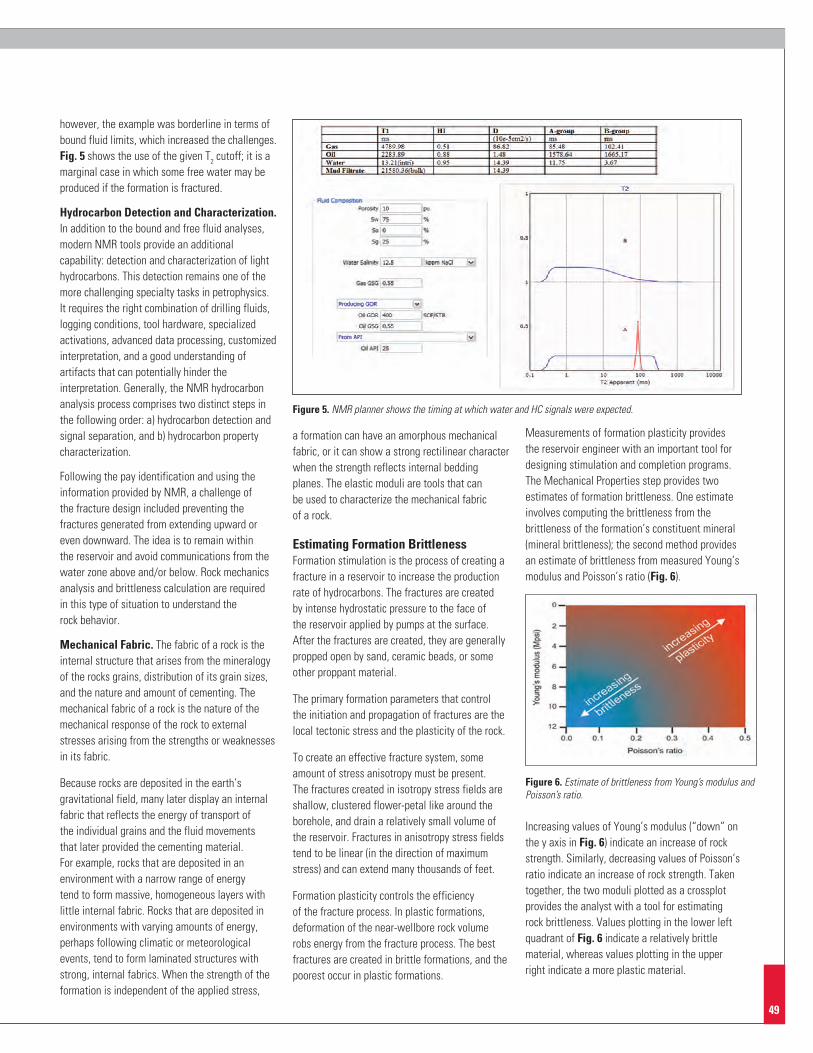
49

Figure 6. Estimate of brittleness from Young’s modulus and Poisson’s ratio.

Figure 5. NMR planner shows the timing at which water and HC signals were expected.

however, the example was borderline in terms of bound fluid limits, which increased the challenges. Fig. 5 shows the use of the given T2 cutoff; it is a marginal case in which some free water may be produced if the formation is fractured.

Hydrocarbon Detection and Characterization. In addition to the bound and free fluid analyses, modern NMR tools provide an additional capability: detection and characterization of light hydrocarbons. This detection remains one of the more challenging specialty tasks in petrophysics. It requires the right combination of drilling fluids, logging conditions, tool hardware, specialized activations, advanced data processing, customized interpretation, and a good understanding of artifacts that can potentially hinder the interpretation. Generally, the NMR hydrocarbon analysis process comprises two distinct steps in the following order: a) hydrocarbon detection and signal separation, and b) hydrocarbon property characterization.

Following the pay identification and using the information provided by NMR, a challenge of the fracture design included preventing the fractures generated from extending upward or even downward. The idea is to remain within the reservoir and avoid communications from the water zone above and/or below. Rock mechanics analysis and brittleness calculation are required in this type of situation to understand the rock behavior.

Mechanical Fabric. The fabric of a rock is the internal structure that arises from the mineralogy of the rocks grains, distribution of its grain sizes, and the nature and amount of cementing. The mechanical fabric of a rock is the nature of the mechanical response of the rock to external stresses arising from the strengths or weaknesses in its fabric.

Because rocks are deposited in the earth’s gravitational field, many later display an internal fabric that reflects the energy of transport of the individual grains and the fluid movements that later provided the cementing material. For example, rocks that are deposited in an environment with a narrow range of energy tend to form massive, homogeneous layers with little internal fabric. Rocks that are deposited in environments with varying amounts of energy, perhaps following climatic or meteorological events, tend to form laminated structures with strong, internal fabrics. When the strength of the formation is independent of the applied stress,

a formation can have an amorphous mechanical fabric, or it can show a strong rectilinear character when the strength reflects internal bedding planes. The elastic moduli are tools that can be used to characterize the mechanical fabric of a rock.

Estimating Formation BrittlenessFormation stimulation is the process of creating a fracture in a reservoir to increase the production rate of hydrocarbons. The fractures are created by intense hydrostatic pressure to the face of the reservoir applied by pumps at the surface. After the fractures are created, they are generally propped open by sand, ceramic beads, or some other proppant material.

The primary formation parameters that control the initiation and propagation of fractures are the local tectonic stress and the plasticity of the rock.

To create an effective fracture system, some amount of stress anisotropy must be present. The fractures created in isotropy stress fields are shallow, clustered flower-petal like around the borehole, and drain a relatively small volume of the reservoir. Fractures in anisotropy stress fields tend to be linear (in the direction of maximum stress) and can extend many thousands of feet.

Formation plasticity controls the efficiency of the fracture process. In plastic formations, deformation of the near-wellbore rock volume robs energy from the fracture process. The best fractures are created in brittle formations, and the poorest occur in plastic formations.

Measurements of formation plasticity provides the reservoir engineer with an important tool for designing stimulation and completion programs. The Mechanical Properties step provides two estimates of formation brittleness. One estimate involves computing the brittleness from the brittleness of the formation’s constituent mineral (mineral brittleness); the second method provides an estimate of brittleness from measured Young’s modulus and Poisson’s ratio (Fig. 6).

Increasing values of Young’s modulus (“down” on the y axis in Fig. 6) indicate an increase of rock strength. Similarly, decreasing values of Poisson’s ratio indicate an increase of rock strength. Taken together, the two moduli plotted as a crossplot provides the analyst with a tool for estimating rock brittleness. Values plotting in the lower left quadrant of Fig. 6 indicate a relatively brittle material, whereas values plotting in the upper right indicate a more plastic material.

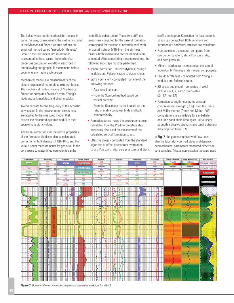
50

The industry has not defined rock brittleness in quite this way; consequently, the method included in the Mechanical Properties step defines an empirical method called “pseudo-brittleness.” Because the rock mechanics information is essential in these cases, the mechanical properties calculation workflow, described in the following paragraphs, is recommend before beginning any fracture job design.

Mechanical moduli are measurements of the elastic response of materials to external forces. The mechanical moduli module of Mechanical Properties computes Poisson’s ratio, Young’s modulus, bulk modulus, and shear modulus.

To compensate for the frequency of the acoustic waves used in the measurement, corrections are applied to the measured moduli that correct the measured dynamic moduli to their approximate static values.

Additional corrections for the elastic properties of the formation fluid can also be calculated. Correction of bulk density (RHOB), DTC, and the various shear measurements for gas or oil in the pore space to water-filled equivalents can be

made (fluid substitution). These two stiffness tensors are computed for the case of formation isotropy and for the case of a vertical well with horizontal isotropy (VTI). From the stiffness tensors, both vertical and horizontal moduli are computed. After completing these corrections, the following sub-steps must be performed:

• Moduli correction - corrects dynamic Young’s modulus and Poisson’s ratio to static values.

• Biot’s coefficient - computed from one of the following methods:

– As a zoned constant

– From the Stanford method based on critical porosity

– From the Gassmann method based on the ratio of matrix compressibility and bulk compressibility.

• Formation stress - uses the overburden stress calculated from the Pre-Interpretation step previously discussed for the source of the calculated vertical formation stress.

• Effective stress - computed from the standard algorithm of effect stress from overburden stress, Poisson’s ratio, pore pressure, and Biot’s

coefficient (alpha). Correction for local tectonic stress can be applied. Both minimum and intermediate horizontal stresses are calculated.

• Fracture closure pressure - computed from overburden gradient, static Poisson’s ratio, and pore pressure.

• Mineral brittleness - computed as the sum of individual brittleness of its mineral components.

• Pseudo brittleness - computed from Young’s modulus and Poisson’s ratio.

• 3D stress and moduli - computes tri-axial stresses in X, Y, and Z coordinates (S1, S2, and S3).

• Formation strength - computes uniaxial compressional strength (UCS) using the Deere and Miller method (Deere and Miller 1966). Computations are available for sand-shale and lime-sand-shale lithologies. Initial shear strength, cohesive strength, and tensile strength are computed from UCS.

In Fig. 7, the geomechanical workflow uses also the laboratory-derived static and dynamic geomechanical parameters measured directly on core samples. Triaxial compression tests are used

Figure 7. Output of the recommended mechanical properties workflow for Well 1.


51

Figure 8. Possibility of cement channels above the fracture zone, which may lead to water production in Well 1.

to determine the static rock properties (Poisson’s ratio and Young’s modulus), and ultrasonic velocity testing is used to determine shear wave anisotropy. Static rock mechanical properties are determined from well-logging data, i.e., crossed-dipole acoustic log data, and calibrated to core analysis results. The orientation of the in-situ stress field along the projected borehole path, from the surface to TD, determines the potential for sloughing and lost circulation. Although the new workflow can determine the magnitude and orientation of these stresses on core samples, it is best determined from acoustic anisotropy analysis using crossed-dipole acoustic logs or from fracture analysis of borehole images. However, because many wells lack dipole acoustic logs and borehole image logs, a composite method for determining mechanical rock properties, using conventional well logs, was developed and validated using core, available dipole sonic log data, and stimulation-treatment pressure-history matching (Mullen et al. 2007). Applying this model in the design of the drill bits, drilling fluid, wellbore

trajectory, and stimulation helps to avoid borehole stability issues, thereby reducing non-productive time (NPT) and improving production. The model uses core-derived data to calibrate the well log evaluation and integrates this data with seismic and geological (mud logs, lithology/mineralogy) information.

Intervals with a higher fracture complexity index (FCI) and higher plasticity provide the best points at which to initiate a hydraulic fracture (Cipolla et al. 2008; Rickman et al. 2008). Model results are used to improve well placement (maximize fracture placement and minimize well instability issues), predict predrill pore pressures, improve drilling efficiency (bit selection, rate of penetration (ROP), borehole quality, and reduce bit trips and NPT) and fluid selection (improves fluid loss control). The integration of the geomechanical model with cement design and stimulation models improves cement integrity and optimizes stimulation effectiveness (wellbore geometry, brittleness index, fracture complexity index,

perforation-interval selection, fracture pressure, fracture fluid, proppant selection, fracture geometry, and proppant selection). When pilot/test or development wells are drilled, diagnostic fracture injection tests (DFIT) are conducted to verify and calibrate this model.

Fig. 8 provides an example of applying the proposed workflow and integrating it with the cement evaluation results to make determinations about the fracture intervals.

This figure shows a possible channel above the tested interval. If the fractures generated during the stimulation process are not contained within the pay interval, then water may be produced from the top zone. Consequently, the rock properties must be understood before beginning the fracturing process.

The recommended petrophysical workflow was applied to the second well and effective results were obtained. The workflow was used to select the zones for stimulation based on the pay criteria applied and the rock mechanic results obtained.

52

Figure 9. Evaluation of Well 2, including the test interval.

The fluid and mineral methodology process was followed to obtain all volumetric data based on probabilistic analysis. The total porosity in this tight sand example was resolved by combining log-measured relative amounts of geochemically derived minerals with the porosity value obtained from NMR. The workflow, as previously discussed, uses a probabilistic error-minimization method to determine the formation fluid and mineral volumes. Tool response equations are expressed in terms of fluid and mineral volumes and their corresponding tool-response parameters. The key component of the analysis lies in only solving for and calibrating to those minerals that are actually found by

core X-ray diffraction (or alternately X-ray fluorescence). Fig. 9 shows the output from Well 2.

Mechanical properties were then calculated following the same workflow in which the conventional vertical Young’s modulus and Poisson’s ratio are calculated from DTC and DTS dipole sonic data. They were calibrated to static rock properties using surface core stress tests and small-volume diagnostic fracture injection tests analysis, then determining fracture pressure, fracture closure pressure, and closure stress gradient. Using the directly measured values of DTC and DTS, calibrated synthetic DTC and

DTS curves can be generated from mineralogy and effective porosity data to use on future wells without actual sonic data when accurate mechanical properties prediction is needed. The differences between vertical and horizontal elastic properties is quantified in a 3D stress analysis requiring fast shear, slow shear, and Stoneley shear data from an oriented dipole sonic log.


53

ConclusionsThis paper discusses the results of a comprehensive logging and formation evaluation workflow conducted in two tight gas wells drilled across a sandstone reservoir in Saudi Arabia. The petrophysical analysis and the testing results led to the following conclusions:

• The analysis method applied enabled and simplified the identification of the best reservoir zones for completion.

• The corrected bin size or T2 cut-off could be adjusted. This adjustment helped to determine the porosity value corresponding to Swi, which does not match the industry average for sandstone. The use of NMR provided a continuous characterization of the well and defined the proportion of the best rock types in the identified gas-bearing sand intervals.

• Integrated formation evaluation using NMR bound fluid, total porosity, and rock mechanics

results enabled many important objectives to be satisfied, including model development, pay selection, water cut prediction, hydrocarbon-water contact identification, and fracture depth interval selection.

• The final composited petrophysical workflow analysis brings the different workflow modules together in a display that helps to identify the primary sweet spot, identifies in-place reserve estimates, and delivers all requirements for an optimized fracture stimulation design. Along the way, it can also generate individual quality control plots and logs from any of its workflow components, enabling transparency of all processes to the end user for further decisions. Advanced 2D NMR analysis facilitates improved hydrocarbon signal separation and in-situ hydrocarbon characterization using the effect of fluid composition on its diffusivity (Meridji et al. 2013).

• Rock mechanics workflow plays crucial role in predicting the sweet spots to be fractured and whether or not the generated fracture would extend upward and/or downward.

• The examination and integration of cement evaluation logs with the petrophysical results, including the rock mechanics, should be performed carefully before proceeding with any stimulation design.

• Proper NMR activation and parameters selections should be performed during the pre-logging job planning phase.

• The ideal NMR logging program includes two activations for exploration/delineation wells, where the open hole section covers thousands of feet. First, a fast bound fluid pass is run through the entire section, providing bound fluid and rock quality indications for reservoir identification and delineation. Second, the fully polarized combined T1 and T2 pass for total porosity and fluid analysis is run in the prospective reservoir sections only.

Figure 10. Rock mechanics of Well 2.

54



Nasreddine Hammou is an Engineer Specialist for the Gas Development Unit of Saudi Aramco. He received his Petroleum Engineering degree in 1995 from the Algerian Institute of Petroleum,

and has been in the oil industry for 18 years. Nasr is registered as a professional geoscientist in Canada, and prior to joining Saudi Aramco in 2012, he worked as a senior staff petrophysicist for Husky Energy Canada.

Ali Belawi is the Supervisor of Gas Development Petrophysics for the Reservoir Description and Simulation Department at Saudi Aramco, where he’s responsible for ensuring that production and

openhole logs are timely analyzed, utilizing the most accurate and complete petrophysics methods. Ali joined Saudi Aramco in August 1989 as a petroleum engineer, and has done extensive work with petrophysics analysis in both exploration and development fields. He holds a BS degree in petroleum engineering from the King Saud University in Riyadh, and is the author of numerous technical papers.

Mahmoud Eid works for Halliburton Wireline and Perforating as the Formation and Reservoir Solutions Manager. He has more than 13 years of experience with Sperry Drilling Services and wireline

logging, including open and cased hole operations, data post-processing and interpretation, and the use of petrophysical software and customer support. Mahmoud spent the last 11 years in Formation and Reservoir Solutions groups in different locations in North Africa and the Middle East assisting logging operations, developing log quality processes, working on special formation evaluation projects and supporting customers’ geosciences asset teams. He is a member of SPWLA and SPE.

Authors

Acknowledgements

The authors would to like to thank Saudi Aramco and Halliburton management for their support and permission to publish this paper.

References

Cipolla, C.L., Warpinski, n.R., and Mayerhofer, M.J. 2008. hydraulic Fracture Complexity: Diagnosis, Remediation and exploitation. Paper sPe 115771 presented at the sPe Asia Pacific Oil and Gas Conference and exhibition, Perth, Australia, 20-22 October.

Coates, G.R., Xiao, L, and Prammer, M.G. 1999. nMR Logging Principles and Applications. Gulf Publishing Co., houston, Texas.

Deere, D.u. and Miller, R.P. 1966. engineering Classification and Index Properties for Intact Rock. Department of Civil engineering, university of Illinois, urbana, Illinois. pp. 90-101.

Melvin, J. and norton, A.K. 2013. Advances in Arabian stratigraphic: Comparative studies of Glaciogenic Juwayl and Lower unayzah strata (Carboniferous-Permian) of saudi Arabia. GeoArabia 18 (1): 97-134.

Meridji, Y., hursan, G., eid, M., and Balliet, R. 2013. Fluid Identification in Complex Reservoirs using 2D nMR Maps: A Case study from saudi Arabia. Paper 599 presented at the sPe Annual Technical symposium & exhibition held in Al-Khobar, saudi Arabia, 19-22 May.

Mullen, M., Roundtree, R., Barree, R., and Turk, G. 2007. A Composite Determination of Mechanical Rock Properties for stimulation Design (What to

Do When You Don’t have a sonic Log) Paper sPe 108139 presented at the sPe Rocky Mountain Oil and Gas Technology symposium, Denver, Colorado, usA, 16-18 April.

Rickman, R., Mullen, M., Petre, J., Grieser, W., and Kundert, D. 2008. A Practical use of shale Petrophysics for stimulation Design Optimization: All shale Plays Are not Clones of the Barnett shale. Paper sPe 115258 presented at the sPe Annual Technical Conference and exhibition, Denver, Colorado, usA, 21-24 september.

reservoir innovations - halliburton.com · the reservoir sediments, comprising alternations of...

Documents