45

RESEARCHES ON SEISMIC HAZARD ASSESSMENT IN RUSSIA

V. I. Ulomov

Institute of Physics of the Earth, Moscow (Russia), E-mail: ulomov@ifz.ru

Abstract To problems of seismicity, seismotectonics and seismic zoning of territory of the country many Russian scientists, including the Institute of Physics of the Earth (IPE) of Russian Academy of Sciences, have devoted their life. Among them such outstanding scientists as B. B. Golitsyn, I. V. Mushketov, and A. P. Orlov. In 2003, the IPE has celebrated the 75-anniversary. In 1991～1997 the new set of General Seismic Zoning probabilistic maps of Northern Eurasia – GSZ-97-A, -B, -C, and -D was prepared on the basis of new methodology and technique. According to these maps, the probability of a possible exceedance of earthquake intensity within 50 years shapes up as follows: 10 percent (map A), 5 percent (B), 1 percent (C), and 0.5 percent (D) which corresponds to the mean return periods of 500, 1000, 5000, and 10000 years for seismic effect. The GSZ-97 maps cover the vast area, including the Russian Federation and adjacent regions of East Europe, Caucasus, Central Asia, Northern Iran, Eastern Turkey, Afghanistan, Mongolia and North China. In 1999 the GSZ-97-A map has been incorporated in 1999 into the World Map of Global Seismic Hazard Assessment. In 2000 the set of GSZ-97 maps was adopted for the area of Russia as the standardizing document and included into the national Building Code “Construction in seismic regions”. The GSZ-97 maps allow to assess the extent of seismic hazard for objects of various lifetime periods and categories of responsibility. In 2002 the Government of Russian Federation has ratified the Federal Program “Seismic safety of territory of Russia” (2002～2010).

1. Introduction

Historical information giving descriptions and interpretations of the nature of individual catastrophic earthquakes in the area of the Russian Empire can be found in archive materials of the 17～18th centuries. But a really scientific approach to seismic phenomena in nature can only be associated with the end of the 19th and the

46

beginning of the 20th century. Prince B. B. Golitsyn was one of the founders of world seismology and seismometry. His name is associated with the creation of the first sensitive seismographs, the beginning of fundamental studies in seismicity and the internal structure of the Earth, as well as the formulation of problems in earthquake prediction. B. B. Golitsyn enriched science with a series of discoveries in the fields of physics and geophysics. He was the first to advance the idea of determining the energy of an earthquake from seismograms and to put forward the method that eventually became classic (Golitsyn, 1912). Co-operating with such prominent scientists as H. Jeffreys, G. Turner, R. Stonely and others, B. B. Golitsyn developed the seismological foundations of instrumental observational seismology on a world scale. In 1911, B. B. Golitsyn was elected President of the International Association of Seismology – predecessor of the present-day IASPEI; and in 1916 he became member of the Royal Society of Great Britain.

The geological basis for studies of the nature of earthquakes were established by I. V. Mushketov and A. P. Orlov (1883) who prepared the first catalogue of earthquakes for the area of the Russian Empire. On I. V. Mushketov’s initiative the Regular Central Seismic Commission attached to the Russian Imperial Academy of Sciences was established in 1900; it contributed significantly to the development of domestic seismology and seismic service. Profound analysis of seismological and geological relationships was continued at the Seismological Institute (the ancestor of IPE, created in 1928) by P. M. Nikiforov and D. I. Mushketov, who identified a series of seismic regions and in 1933 published the first zoning map of Middle Asia. In 1937, the first standard map of seismic zoning for the whole area of the former USSR was published by G. P. Gorshkov, who initiated regular compilation of such maps as the basis for regulating and design construction in seismic regions.

The problem of seismic zoning, in close connection with earthquake prediction, started to be systematically developed in our country on the initiative and under the leadership of G. A. Gamburtsev in 1949 immediately after the 1948 Ashkhabad catastrophe (Turkmenistan). Already then, G. A. Gamburtsev clearly formulated the goals and tasks of multidisciplinary researches in this most important scientific and social problem. Being a founder of new methods for seismic prospecting of the Earth’s interior (Deep Seismic Sounding – DSS) and correlation methods for earthquake study (CMES), G. A. Gamburtsev (1955) considered the nature of seismic processes in their intimate association with geological environment, with its deep structure and dynamics. At the same time the Siberian seismogeologists (N. A. Florensov, V. P. Solonenko, V. S. Khromovskikh) developed and actually used new paleoseismological methods for the identification of traces of ancient earthquakes, namely, paleoseismodislocations, which began to be widely incorporated in the study of seismicity in the area of Russia and other regions of the world.

In mid-1950s S. V. Medvedev (1947), I. E. Gubin (1950), G. A. Gamburtsev (1955), Yu. V. Riznichenko (1965) and other Russian scientists laid the foundations of the two-stage seismogenic method for estimating seismic hazard with some elements of prediction. In accordance with this concept, actual and potential source zones are identified at the first stage, while the expected effects on the Earth’s surface are calculated at the second stage. However, practically all

47

the previous maps of General Seismic Zoning (GSZ-1937, -1957, -1968 and -1978) were deterministic and took no account of the main characteristics of seismicity in the seismic regions, although as long ago as in the mid-1940s S. V. Medvedev proposed using an internal differentiation of seismic hazard zones based on the return period of large earthquakes and assumed lifetimes of different types of building objects.

Yu. V. Riznichenko, in developing the ideas of a probabilistic approach to seismic zoning, proposed a method for calculating “shakeability”, defined for every point of the Earth’s surface as the average annual number of shaking episodes caused seismic intensity equal to or greater than a certain fixed level. For the first time, a quantitative probabilistic measure of seismic hazard was introduced into seismological practice. But for various reasons, paradoxical though it may seem, the new advanced method has been used for GSZ maps, neither in 1968 nor in 1978. Eventually, each map proved to be, to some or other extent, inadequate to the actual conditions, which added to low-quality construction, of caused great material loss to the national economy and caused the loss of numerous human lives. These maps, like the two previous ones (1937, 1957), continued to be based only on deterministic expert assessment of seismic hazard. At the same time, similar probabilistic method for seismic zoning began to be applied widely immediately after the paper published by American scientist C. A. Cornell (1968).

The contemporary level attained by the world science of earthquakes and the conditions of uncertainties always existing in nature render deterministic seismic zoning inappropriate. Seismic zoning can only be carried out on a probabilistic basis. In other words, there will always exist some risk but it should be minimized. Such an approach to the assessment of seismic hazard and seismic zoning of regions is used as the basis for contemporary research in many countries of the world.

The 1991～1997 researches headed by the author covered the area not only of the Russian Federation, but also of all the CIS countries and adjacent seismic regions, as well as the shelves of marginal and inland seas. The chief features that distinguish the new methodology and technique from the previous methods for seismic zoning are: the development of a common (for the entire area of Northern Eurasia) and adequately parameterized model of earthquake sources; taking into account various nonstandard information on regional seismicity (fractal structure of the environment and of seismic processes, nonlinearity of the magnitude-frequency relations and the attenuation of seismic effects with the distance and so on) and the information on seismic sources (their size, orientation, moment magnitudes, stress drops, distribution of sources throughout the seismic layer rather than at a fixed depth, as previously, and so on).

Our researches of General Seismic Zoning relied on the principle of design seismic excitation with a fixed return period. As a result, the set of probabilistic maps was compiled of seismic zoning of the area of Northern Eurasia – GSZ-97 (instead of one map, as previously) designed for engineering objects of various critical categories and lifetimes and reflecting a design intensity that is equally probable for a concrete level of risk (Ulomov, 1993a, 1994, 1997, 2000, 2002; Ulomov and Shumilina, 1999; Gusev et al., 1998; Gusev and Shumilina, 2000).

48

2. Seismogeodynamics and Seismicity of Northern Eurasia

2.1．Global orderliness of seismic regions

Structural and geodynamic laws of tectonics, characteristic for the vast territory of Northern Eurasia, allows to consider it as a planetary seismogeodynamic system (SGD-system). These laws are clearly displayed in the hierarchical heterogeneity of tectonic structures starting from the lithosphere and finishing with blocks of the Earth’s crust of various ranks, as well as in the trend of their geodynamic development.

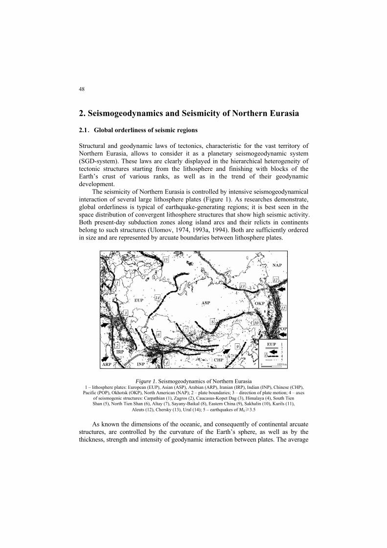
The seismicity of Northern Eurasia is controlled by intensive seismogeodynamical interaction of several large lithosphere plates (Figure 1). As researches demonstrate, global orderliness is typical of earthquake-generating regions; it is best seen in the space distribution of convergent lithosphere structures that show high seismic activity. Both present-day subduction zones along island arcs and their relicts in continents belong to such structures (Ulomov, 1974, 1993a, 1994). Both are sufficiently ordered in size and are represented by arcuate boundaries between lithosphere plates.

Figure 1. Seismogeodynamics of Northern Eurasia 1 – lithosphere plates: European (EUP), Asian (ASP), Arabian (ARP), Iranian (IRP), Indian (INP), Chinese (CHP), Pacific (POP), Okhotsk (OKP), North American (NAP); 2 – plate boundaries; 3 – direction of plate motion; 4 – axes

of seismogenic structures: Carpathian (1), Zagros (2), Caucasus-Kopet Dag (3), Himalaya (4), South Tien Shan (5), North Tien Shan (6), Altay (7), Sayany-Baikal (8), Eastern China (9), Sakhalin (10), Kurils (11),

Aleuts (12), Chersky (13), Ural (14); 5 – earthquakes of MS≥3.5 As known the dimensions of the oceanic, and consequently of continental arcuate

structures, are controlled by the curvature of the Earth’s sphere, as well as by the thickness, strength and intensity of geodynamic interaction between plates. The average

49

statistical length of convergent regions of the world is about 3000 km, and their width some hundreds kilometers. The distances between these structures change in a relatively wide range and depend on their age and the deformation features of the host rocks. In continents these arcuate structures are the most congested and are deformed more irregularly, while in offshore conditions they exhibit more regular geometrical forms. Present-day subduction zones, as well as their relicts in continents, are characterized by reduced strength and high mobility as compared with the contiguous more consolidated rocks. Precisely this fact is responsible for their high seismic activity.

The predominant number of Northern Eurasia earthquakes occur in the upper crust at depths down to 15 km. The distribution of their hypocenters is controlled by the hierarchical fractal structure of the Earth and by the sizes of the earthquake sources themselves related to the magnitudes of corresponding earthquakes. The Kuril-Kamchatka subduction zone with the depth of hypocenters in excess of 600 km is the most mobile and seismically active region of Northern Eurasia. It is here that the largest earthquakes occur and the bulk of seismogeodynamic deformation and seismic energy in the area of study is released. Earthquake sources with intermediate depth are characteristic of two well defined relict subduction zones: the Vranchea zone in the Eastern Carpathians (as deep as 200 km) and the Pamir–Hindu Kush zone in Central Asia (down to 300 km). The earthquakes with depth up to 150 kilometers take place in the Northern Caucasus and central part of Caspian Sea.

(a) (b)

Figure 2. The seismic rate (a) and cumulative distribution of seismogenic lineaments (b) in different regions of Northern Eurasia

1.1 – Iran-Caucasus-Anatolia; 2.1 – Pamir-Tien Shan; 3.1 – Altay-Saiany-Baikal; 4.1 – Kurils; 4.2 – Sakhalin; 4.3 – Amur area; 4.4 – Chersky; 4.6 – Chukotka; VR – seismic rate, Nj – number of lineaments of different ranks

(MS) in each region, and Σ – for whole Northern Eurasia (see below LDF model) The seismicity of every region and the magnitudes of the largest possible

earthquakes in it have a direct bearing on the dimensions of regional earthquake-generating features, its geological age and hierarchical fault block structure, strength spatial location and the trend of geodynamic development in the region. In spite of similar origins, each region has a tectonically individuality of its own, contains genetically interrelated earthquake-generating features of different ranks, and is characterized by a seismicity of its own (original “seismogeokainos”). Therefore,

50

precisely regions of the dimensions referred to above (about 3000 km in length) are assumed to be the basic earthquake-generating unit for developing the model of earthquake source occurrence (ESO) zones and its seismological parameterization.

Each region is characterized by the nonlinear plot of return periods of earthquakes with different magnitude (Figure 2a). Straight segments of the plots with a slope b≈-0.9 are characteristic only of the magnitude 4.0≤M≤6.0 (for the magnitude M it is designated as MS). However, starting from magnitude M≥6.5, all plots indicate a higher frequency of these earthquakes than was to be expected from a linear extrapolation of the left part of the plots to the right. The nature of such a phenomenon is, first of all, due to the occurrence of earthquakes of different magnitudes in environments differing in physical properties which vary significantly with depth. Not only seismological, but also geological information, obtained by studies of paleoseismodislocations and used in seismic zoning, indicate the high frequency of large earthquakes (Ulomov, 1974; Wesnousky et al., 1984; Schwartz and Coppersmith, 1984; Youngs and Coppersmith, 1985; Wesnousky, 1990; Gusev et al., 1998; Ulomov and Shumilina, 1999; Gusev and Shumilina, 2000).

Figure 2b illustrates the cumulative distribution of the number of seismogenic lineament structures of different ranks in same regions of the Northern Eurasia (explanations look below on LDF-model). The necessity of constructing cumulative plots is explained by the fact that lineaments of maximum magnitude (Mmax) include also lineaments of lesser ranks since earthquakes of M＜Mmax occur among them too. The distribution of lineaments with different ranks over Mmax for regions is an overall reflection of the fractal dimension Uj ≈-0.9 for the entire hierarchical set of lineaments, which is consistent with the b≈ -0.9 (Figure 2a). Indeed, both sets of curves (b-value and U-value) for the magnitude range М≥ 6.0 have similar configurations as well, thus corroborating the idea of nonlinear magnitude-frequency relations and of a structural-dynamical unity of the geophysical medium and the seismic processes going on in it.

The actual frequency of large earthquakes in Northern Eurasia is three and more times higher than previously assumed. The use of straight plots in past years resulted in significant overestimation of the return time of large earthquakes, hence, in underestimation of seismic hazard practically in all the regions of the former USSR.

2.2．Regional orderliness of seismogenic structures

The seismogenic faults and earthquake sources are not distributed chaotically. The fault ranks, and the distances between their dislocated nodes (or segments) as well as geoblock sizes are determined by the thickness and strength of the related layers faulted in the past geological epochs. The thicker the layer divided by faults into blocks, the larger and longer the faults and the greater the distances between them. The larger the blocks, the more magnitude of earthquakes connected to them. Conversely, the number of faults, blocks and earthquake sources increase as the layer thickness decreases.

51

It was found that distances between faults and accordingly the dimensions of blocks exhibit a well-pronounced tendency of clustering in ranks, their vertical and horizontal dimensions being in a ratio of roughly two to one between adjacent ranks (Ulomov, 1974, 1993a, 1994). This phenomenon seems to have its origin in the persistent doubling of the depths to major discontinuities in the crust and upper mantle, the faults of respective ranks penetrating as deep as the discontinuities. To take an example, the top of the “granite” layer in the continents lies at a mean depth of ∼10 km, the Conrad discontinuity is at 20∼25 km, the crust-mantle interface (Mohorovičič discontinuity) is at 40∼50 km, the bottom of the lithosphere at ∼100 km, that of the asthenosphere at ∼200 km, these being followed by the ∼400km and ∼700km discontinuities. This fundamental pattern of discontinuous change in material properties as the depth is multiplied by two governs all geological depths up to and even including the soil.

The orderliness thus emerging dictates a corresponding orderliness, not only in systems of tectonic faults and geoblocks, but also in the hierarchy of earthquake sources: the larger the earthquakes, the farther their sources from one another. Thus, earthquake sources when ranked according to magnitude M are distributed in a regular manner, not only in time (“magnitude-frequency relation”), but also in space (“to keep the distance”). It has turned out that the mean distances δ M (km) between the epicenters of two closest-lying earthquake sources of length LM (km) and magnitude M are well described by the following relations:

)94.16.0(M 10 −= Mδ (1)

)5.26.0(M 10 −= ML (2)

As is apparent, the factor 0.6 at M implies that the source sizes LM and distances between epicenters δM change approximately by a factor of two with 0.5 increase in magnitude. From the above relations it follows that the quantity δM/LМ = 3.63 is an invariant in relation to magnitude, reflecting self-similarity in the size hierarchy of geoblocks and the associated earthquake sources in the entire magnitude ranges (Ulomov, 1987). Also invariant of magnitude, to some degree at least, is the ratio of earthquake sources length LM to the vertical sources plane extent HM, which is identical with the respective thickness of the geoblocks.

The quantity δM is none other than the mean horizontal size (diameter) δj of geoblocks that can generate earthquakes of the respective maximum magnitude Mmax; δjM is the diameter of the area responsible for Mmax, a very important quantity for the assessment of earthquake hazard; this is related to δj as follows:

Mmax = 1.667 lg δj + 3.233 (3) The important conclusion follows from here: realistic magnitude-frequency

relations should be made only for areas which size (diameter) should be no less than quadruple size LM of earthquakes with magnitude Mmax.

Interrelationships in the orderliness of faults, geoblocks and earthquake sources, as well as in the evolution of seismogeodynamic processes are just more evidence in favor of a structural and dynamical unity of the hierarchical geophysical medium and

52

the SGD processes that are going on in it. Orderliness obtains also in the hierarchy of soliton-like strain waves (called by the author G waves, or geons) of seismicity increases (Ulomov, 1987, 1993b). These provide for the dynamics of interacting geoblocks and for directivity in the evolution of synergetic SGD processes. Geons propagate along faults of their respective ranks, creating and removing various barriers and therefore provoking earthquake sources of appropriate magnitudes. Since these geodynamical processes are evolving more or less independently at each hierarchical scale, they possess the same fractal dimension as for the fault-blocky medium and its seismic regime. When the external geodynamical excitations are low, the seismicity in the region is close to the steady state, involving small shallow earthquakes that are being generated by a denser network of smaller faults. When the external forces become greater, e.g., as a result of major coseismic or creep movements, the SGD system passes to a qualitatively different and better organized state. Larger fault zones begin to “operate”. This can be inferred from ordered changes in seismic activity in many regions worldwide (migration of earthquake sources, periodic seismic rate increases, localization of quiescent areas and the like) which are caused by synergetic self-organized phenomena typical of many hierarchical multicomponent non-equilibrium systems.

3. Methodology of Seismic Hazard Assessment

3.1．The new approach to the assessment of seismic hazard

The new study of seismogeodynamics and seismic zoning is based on the new methodology and homogeneous database. The first time, uniform seismological and geological-geophysical electronic database was created for the entire vast area of Northern Eurasia, including Russia and other CIS countries as well as the adjacent seismic regions and shelves of marginal and inner seas.

The main advantages of the methodology and the relevant software are as follows:

The new regional approach to the development of the model of earthquake sources, providing adequate seismological parameterization of earthquake source zones (estimation of magnitude of maximum possible earthquakes, adequate seismicity parameters and so on);

Presentation of the earthquake recurrence plots for different magnitudes, not in the form of simple exponents, as before, but by incorporating various data on seismicity and seismogeodynamics (including information on the age of paleoseismodislocations, historical chronicles and so on);

Presentation of the earthquake sources, not as abstract points, but in accordance with their natural dimensions, orientation in space, depth distribution, etc.;

Using of the values of stress drops, seismic moments M0, moment magnitudes MW (instead of traditional MS and MLH) and other quantitative parameters to characterize the energy of an earthquake source;

Description of the field of incoherent radiation near an extended source, which

53

has enabled to resolve the problem of overestimated design seismic intensity at short distances from the epicenter and to simulate the realistic form of isoseismals in the near zone due to the extended sources of high magnitude earthquakes;

Introduction of a probabilistic approach to estimation of the reliability of various results and input data (scatter of seismic intensity at given magnitude and distance, fluctuations of the slope angles of planes of lineament structures, distribution of sources over depth and so on) at all the stages of investigation;

Compilation of a set of maps (instead of one map, as previously) of probabilistic seismic zoning, which have since been used in the practice of earthquake-resistance construction of objects of different categories of importance and lifetimes.

Figure. 3 shows the diagram of the methodology of our researches to produce the set of General Seismic Zoning maps for the area of Northern Eurasia (GSZ-97). The concept is put in basis on the representations about structural-dynamic unity of the geophysical environment and seismic processes proceeding in it – in essence, and probabilistic-deterministic representations – under the form (Ulomov, 1993a).

Figure 3. Diagram of the methodology of seismic zoning On the basis of three database blocks (recent geodynamics, regional seismicity

and strong ground motion), two models are created: the Source Zones Model (SZM)

54

and the Seismic Effect Model (SEM) which are used to calculate seismic hazard and to make seismic zoning maps.

Fixation of the huge material in a digital electronic form within the Geographical Information System (GIS) is a distinct fundamental achievement of the new technology of seismic hazard assessment as compared with all previous methods used in former USSR. It permits obtaining rapidly reference analytical information on all the parameters and to use the materials for the preparation of maps of larger scales on their basis, as well as to estimating the seismic hazard, the seismic risk and vulnerability of specific regions and countries.

In case some additional data is revealed on seismic hazard (the discovery of hitherto unknown paleoseismodislocations, of new historic information on past earthquakes, of the migration of seismic activity and so on) the database allows for rapid incorporation of any necessary corrections into the calculations of seismic hazard and, correspondingly, into its mapping.

3.2． The Lineament-Domain-Focal model of earthquake source zones

Earthquake hazard is defined as the probability of maximum ground motion intensity due to all potential seismic sources in the region not exceeding a specified limit during a fixed period of time. The identification of Earthquake Source Occurrence zones (ESO zones) and the determination of seismicity parameters for them is the most complex and crucial part in seismic hazard assessment, because this determines the trustworthiness of all subsequent developments. The sources are usually modeled by a set of points, lines and other elementary geometrical figures, which allows geometrically regular phenomenological seismogenic models to be successfully used for seismic zoning. One example is the Fractal Lattice Model (FLM) for the space-time and energy evolution of intracontinental SGD processes proposed by this author in the mid-1980s (Ulomov, 1987). The FLM is based on the natural hierarchical structure of geologic features, geodynamic processes and, consequently, earthquake sources.

The basis for the model of ESO zones for seismic zoning is the Lineament-Domain-Focal (LDF) model modified from FLM (Ulomov, 1998).

The LDF model contains four scales (Figures 4 and 5): a major region (R) with an integral characteristic of common seismicity and its three main structural elements: lineaments (lΜ), which roughly represent the axes of the tops of 3-D earthquake-generating fault features and are characterized by structured seismicity; domains (dΜ), which cover the area without gaps and are characterized by scattered seismicity; potential earthquake sources (sΜ) indicating the most dangerous segments and which are generally confined to lineaments. The “driving force” in the LDF model comes from interaction between geoblocks and from the above mentioned “geons” which accommodate movements of block sides.

Lineaments, domains, and potential sources are classified by maximum possible magnitude Mmax, as are the earthquakes, at intervals: M=8.5±0.2, 8.0±0.2, 7.5±0.2, 7.0±0.2, 6.5±0.2, and 6.0±0.2. According to the LDF model each lineament with Mmax also includes all smaller ones, down to M = 6.0 (see Figure 2)

55

which deviated from lineament axes for value D reversely proportional to earthquake magnitude М (see Figure 4).

The upper magnitude Mmax is controlled by the relevant seismogeodynamic environment, while the lower Mmin is determined by completeness of reporting for earthquakes with the lowest magnitude that still poses some seismic hazard (usually Mmin= 4.0 and the lowest intensity of shaking being Imin = 5 of MSK-64 or EMS-98 scales).

Figure 4. Illustration of the LDF model of ESO zones 1. – axial planes of lineament structures l(Mmax); 2. – outlines of domains d; 3. – observed active faults; 4. – earthquake sources L(Mmax) with magnitude М = 6.0 and more, that deviated from lineament axes for value D reverse proportional

to earthquake magnitude М (see background plot, σ – standard deviation); 5. – earthquake sources with magnitude М = 5.5 and less, randomly scattered within the domains

Figure 5. Model of seismicity and seismic regime for region (R) and its main structure elements – lineaments (l), domains (d), and potential sources (s)

The magnitude-frequency relations for each type of feature are shown: VR – a mean yearly earthquakes rate in the entire region, Vl – in the lineaments, Vd – in the domains, and Vs – in the potential earthquake sources

56

The magnitude Mmax is assessed by all accessible and reasonable techniques: from the dimensions (δ j, km) of interacting geoblocks, the width of zones of dynamical influence emanating from major seismogenic features, the length and segmentation of earthquake-generating faults, from archeological and historical evidences, the configuration of the magnitude-frequency relation, the extreme values in the plot of strain buildup in seismogenic features, the positions of potential earthquake sources likely to produce the maximum magnitude, and also from the dimensions of paleoseismodislocations (Lsd, km) according to the following relation, for example:

Mmax = 1.667 lg Lsd + 4.167 (4) In order to identify the structures generating seismic waves and to estimate their

seismic potential, it is important to use the mapping of the sources of earthquakes with various magnitudes in accordance with their size and orientation rather than the mapping of abstract “point” epicenters as is commonly done. The size and orientation of source are determined from the distribution of aftershocks, coseismic ruptures, configuration of maximum isoseismal lines, focal mechanisms, geodetic measurements, analysis of tectonic events, and so on. In accordance with the new map legend, sources of earthquakes with M ≥ 6.8 are shown as ellipsis of corresponding size and orientation. The large L and small W axes of the ellipsis, as well the conventional diameters L' of circles for weaker sources are correspond to the following equations:

16.024.0lg:7.6;42.015.0lg ;5.26.0lg:8.6

−=′≤+=′−=≥

MLMMWLMLM (5)

Seismolineaments serve as the main carcass for the LDF model of ESO zones and represent in a generalized form the axes of the upper edges of the three-dimensional and relatively clearly structured (concentrated) seismicity at the Earth's surface (see Figure 4). They trace the geoblock boundaries, which are characterized by the most contrast tectonic activity. Lineaments are identified by cluster analysis of the space-time distribution of earthquake sources of corresponding magnitudes, as well as from the geophysical fields (especially from their gradients), from paleoseismodislocations, cosmic photographs, from the similar historic-tectonic development in the Cenozoic era (predominantly in the upper Pleistocene and Holocene), from activity in the Quaternary period, from the close values of velocity gradients of neotectonic movements and from other signs of recent geodynamics. Lineaments and their segments are characterized by the magnitude Mmax of the maximum possible earthquake; by their length li and width wi due both to their tectonic nature and the errors in determining their dislocation; by the depth of bedding of the upper, hmin, and lower, hmax, edges of the plane of seismogenic structure; by the strike azimuth Az0; by the dip angle α0; by the type of predominant displacements (shear-fault, normal fault and so on). Lineaments can exhibit strikes of most diverse types due to the tectonics of a region and can intersect each other, which “automatically” increases the seismic hazard in their dislocated nodes in calculations owing to seismic effects from the summing up of nearby located sources.

Domains (dΜ) are volumetric areas less pronounced as far as structure is concerned

M≥ M≤

57

or inadequately studied seismogenic zones characterized by “quasi-homogeneous” tectonics and relatively weak seismicity. They embrace layers of thickness from hmin to hmax kms. Unlike lineaments, domains do not intersect each other, and they cover all the investigated territory without breaks and superposition. An apparent intersection is characteristic of domains belonging to different depth layers, i.e. in the subduction zones and their relict on the continents (for example, Hindu Kush, Eastern Carpathians, Caucasus and in other regions). As it has been mentioned, the “domain” concepts (as well as the concept of “quasi-homogeneous” seismotectonic provinces) is the cost related to difficulties, associated with revealing the more fine structure of focal seismicity from weak earthquakes, due to errors in determining the locations of their epicenters. Actually, there is no doubt that focal seismicity is structured at all scale levels.

Potential Sources (sΜ ) of earthquakes identified by various methods (from dislocations, from the dominant distances between epicenters, by methods of pattern recognition, and so on) are, as a rule, confined to lineaments, and their dimensions Ls are related to the magnitude of the maximum possible earthquakes. Potential sources have the same parameters as the respective lineaments.

According to the LDF model, as was pointed out above, each lineament that can generate earthquakes of Mmax also includes lineaments of smaller ranks, down to M = 6.0 inclusive, because these also produce (with some deviations across the feature) earthquakes of lower magnitudes as well. Events of Mmax≤5.5 generally belong to domains. Potential earthquake sources have definite magnitudes (usually Mmax≥7.0) and most frequently occur on lineaments.

Since the actual earthquake sources do not occur strictly along lineament axes, but deviate from these in some way, it is possible to calculate the mean deviations (see Figure 4). The lower the magnitude, the farther the sources may stray from the relevant lineament axis. It is useful for bringing the model closer to what is actually observed in nature.

According to the LDF model, the top of the associated sources reach (but do not go beyond) the top of the consolidated crust, although the earthquake sources themselves and the associated hypocenters involve a greater scatter in depth of focus, since the depth distribution of larger earthquakes is controlled by the vertical extent of the source planes. In addition to nearly vertical sources planes (90°±20°) usual on strike slip faults, lineaments are characterized also by two different ranges of dip, 45°±20°and 135°±20°for thrusts and for normal faults. The resulting characteristics of seismicity behavior and the scatter of earthquake sources are further used in subsequent work to model a predicted (virtual) seismicity, to calculate repeat times of intensity in seismic zoning.

3.3．Seismological parameterization of earthquake source zones

The basic quantity in calculating seismicity parameters for the main structural elements of ESO zones is the total rate of seismic events VRM per one year in region (Figure 6).

Since the seismic regime of any structural ESO element (lM, dM, sM) is controlled by the common rate in the region the plots of Vl, Vd, Vs in each element will be

58

absolutely identical with it when summed over all elements (“the law of conservation of seismic energy”):

ΣVlм+ΣVdм+ΣVsм =VRM (6) Seismological parameterization of each lineament (segments of lineaments as

well) requires the total length (ΣlМ) to be calculated for each region; this consists of the lengths ΣlМof all lineaments of this and higher ranks, since, as mentioned above, lineaments with Mmax also include all those with M＜Mmax down to M = 6.0. The next step is to find the mean yearly rate Vlм for the events of the relevant magnitude along each lineament (and segments of these) lM in length as being part of VRM, which is the total rate of seismic events with this magnitude in the region:

Vlм = VRM lМ / ΣlМ (7) The rate of seismic events in a domain, VdM, is simpler to find: this is based on a

selection from the standardized catalog of all M≤5.5 events occurring in the domain of interest and plotting the associated magnitude-frequency relation. It goes without saying that the law of conservation of seismic energy must hold in this case too, because the rate of events in a domain is also part of the total rate (VRM) in the region for the magnitude range 4.0≤M≤5.5. Expert assessment is at present used for aseismic or low seismicity regions.

The rate VSм at potential sources is defined as the part of Vlм on the relevant lineaments, but the earthquakes taken into account here are only those with this particular magnitude M = Mmax rather than the total rate with M＜Mmax as is the case for ordinary lineaments, i.e., excluding the regular background seismicity for the relevant lineament segment and the aftershocks of the potential sources.

Figure 6. Illustration of the distribution of annual regional seismic rate VR of different magnitude M between lineaments, domains and potential sources in the region. The total rate of events in region

should correspond to the full rate in whole genetically uniform region It should be noted that the identification and adequate seismological

parameterization of lineament structures play the important role for reliable estimation of seismic hazard. The representation of seismogenic structures only as

59

“quasi-homogeneous seismotectonic provinces” (“domains” in our terminology) with their scattered seismicity, which has been widely accepted until recently, is less realistic from both the seismological and geotectonic standpoints. Although the scattered seismicity does not actually exist in nature, seismologists are compelled to use such an approach, as well as the domain (“seismotectonic province”) model, because a knowledge of the fine structure of the seismic medium is incomplete. In this respect, the most rational way is to construct a hybrid lineament-domain model which is presented in this paper. However, the overall replacement of high-amplitude lineaments by areal domains is unacceptable for physical reasons. Moreover, this is unjustified for the following two reasons. First, a decrease in the domain area without regard to the size of zones responsible for large earthquakes increases the recurrence period of such events and, consequently, underestimates the seismic risk, resulting in errors of the “missing target” type in seismic zoning maps. Second, an excessive enlargement of the domains within which high-magnitude earthquakes are possible makes the seismic risk pattern more diffuse and gives rise to errors of the “false alarm” type.

The lineament-domain-focal model of ESO zones, based on the probabilistic-determinate fractal lattice regularization of the parameters of regional seismicity and recent geodynamics avoids these shortcomings and adequately incorporates the specific features of the distribution of earthquake sources for various magnitudes.

The new method of creation of earthquake source zones model and their application to the seismic zoning was named by us “Earthquake Adequate Source Technology − EAST-97” (Ulomov et al., 1999). Now the software for GSZ is modernized and automated. It is named EAST-2003 and became accessible to all users.

3.4．Virtual seismicity and model of seismic effect

Figure 7 illustrates the GSZ technology on the example of the Caucasus and adjacent area. Figure 7a shows the observed earthquake sources of different magnitudes and sizes LM: M=8.0±0.2 (large ellipses 200 km long); M=7.5±0.2 (medium ellipses 100 km long); M=7.0±0.2 (small ellipses, 50 km); M=6.5±0.2 and less, at intervals of 0.5 magnitude units (circles of decreasing diameter from 25 km).

The LDF model shown on a Figure 7b is created on the basis of observed regional seismicity, seismotectonic and seismogeodynamic of this area. Here are shown: l—seismogenic lineaments with Mmax = 8.0±0.2; 7.5±0.2; 7.0±0.2; 6.5±0.2; 6.0±0.2 (line thickness decreasing by a factor of two for the respective magnitudes); d — domains having different Mmax ≤ 5.5; s — potential sources with size Ls corresponding LM.

Figure 7c shows an example of predicted seismicity for this region obtained by computer generation of virtual earthquake sources based on a synthetic catalog generated in accordance with the LDF model and corresponding seismic regime in this region. This catalogue is compiled from the given long-term characteristics of seismicity in a region. Its duration must be adequate for reliable estimation of return period of intensity occurrence. Each event in the catalogue is characterised by

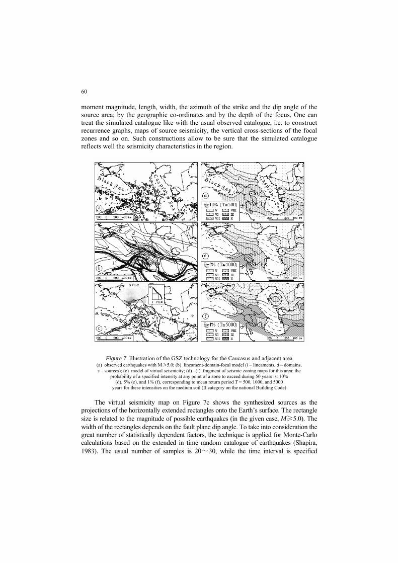
60

moment magnitude, length, width, the azimuth of the strike and the dip angle of the source area; by the geographic co-ordinates and by the depth of the focus. One can treat the simulated catalogue like with the usual observed catalogue, i.e. to construct recurrence graphs, maps of source seismicity, the vertical cross-sections of the focal zones and so on. Such constructions allow to be sure that the simulated catalogue reflects well the seismicity characteristics in the region.

Figure 7. Illustration of the GSZ technology for the Caucasus and adjacent area (a) observed earthquakes with M≥5.0; (b) lineament-domain-focal model (l – lineaments, d – domains, s – sources); (c) model of virtual seismicity; (d) –(f) fragment of seismic zoning maps for this area: the

probability of a specified intensity at any point of a zone to exceed during 50 years is: 10% (d), 5% (e), and 1% (f), corresponding to mean return period T = 500, 1000, and 5000

years for these intensities on the medium soil (II category on the national Building Code) The virtual seismicity map on Figure 7c shows the synthesized sources as the

projections of the horizontally extended rectangles onto the Earth’s surface. The rectangle size is related to the magnitude of possible earthquakes (in the given case, M≥5.0). The width of the rectangles depends on the fault plane dip angle. To take into consideration the great number of statistically dependent factors, the technique is applied for Monte-Carlo calculations based on the extended in time random catalogue of earthquakes (Shapira, 1983). The usual number of samples is 20～30, while the time interval is specified

61

depending on the assigned probability of exceeding (or non-exceeding) for expected earthquake hazard. In Figure 7c one such sample is shown only. The two maps (Figure 7a and Figure 7c) look similar, demonstrating that the LDF model of ESO is realistic.

The final phase of seismic hazard assessment involves calculation of seismic effects at the Earth's surface due to each individual virtual source taking into account its dimensions and the attenuation law of seismic ground motion. The calculation of effect is carried out for each node of grid with size 25km×25 km (or other, depending on scale of a map and desirable detail) covering the region and adjacent area. For each node (“receivers”) of grid a histogram of intensity occurrence is made, these data being the basis for subsequent mapping of earthquake hazard and related tasks. A histogram and a fragment of this grid can be seen on the Figure 7c.

Figure 8. A schema for calculation of seismic intensity from a single source (after Gusev and Shumilina, 2000)

C, C′ − hypocenter and epicenter of the rectangular source of length L and width W on depth H, inclined under a corner φ; XY − Earth's surface; P − point of supervision (“receiver”); r − hypocentral distance, rj − distance up

to j-subsource (“radiator”), on which is broken the source; the rectangular on a plane XY − projection of the source to earth’s surface, bold edge − projection top of the source; ellipses on the plane XY − contour lines

of seismic effect from the given source The length and width of the rectangle and their relationship depend on the

moment magnitude MW and the stress drop. The hypothesis of geometric and dynamic similarity of sources is applied for prediction of the parameters of the rectangular area from the moment magnitude. Deviation from this hypothesis is also modeled. The scatter of stress drop is modeled as a random value and the length-width relationship as a deterministic function of magnitude. The real scatter of intensity for a given magnitude is modeled at the point of observation on the basis of the hypothesis of a normal law for the error in the prediction of intensity according to the adopted calculation scheme. The value of the standard deviation of this law is given. The

62

model takes into account saturation effects of the intensity near the source, the nonlinearity of the intensity-distance relationship and saturation of the magnitude for large seismic moment M0 , i.e. the problem of overstating the intensity for small distances and the seismic effect in the form of an ellipse is modeled automatically within the near zone for the sources of large magnitudes (see Figure 8).

The intensity–magnitude–distance relationship I(MW, D) is modeled from the regional empirical data (Figure 9). To approximate these data and to predict the intensity, the model of such a relationship is used that assumes the idea of an incoherent extended source in the form of a radiating rectangle with its long side parallel to the Earths’ surface (Gusev, 1984; Gusev and Shumilina, 2000).

Figure 9. The intensity-magnitude-distance relationship I(MW, D)

As a parameter suitable for prediction of the intensity, the integral of the square

of an accelerogram, or the “Arias intensity”, is applied (Arias, 1970): ( ) ttaA d 2∫= (8)

This is a modification of the approach described in Aptikaev and Shebalin (1988):

502 daAAiii = (9)

Here a(t) is the accelerogram; a is the maximum acceleration; d50 is the duration of the part of the accelerogram with amplitudes exceeding 50% of the maximum.

The relationship between intensity and physical parameters of the oscillations of ground is accepted in the following form:

I = CAlgA+const (10) where CA=1.667 taking into account the usual relation dlga/dI= lg2 and in accordance with I=3.33lg(ad50

0.5 ) + const. The idea has been used of additive of the energy contributions of elementary

radiators (subsources) – the components of a source forming the field in a receiver. It is assumed that the source is a limited area, the elements of which emit high-

D(km)

63

frequency (short-period) radiation independently (incoherently). This means that the energy contributions of different elements of the area are summarized in the receiver, and that at some receiver point:

( ) ( )tataN

ii∑

=

=1

22 ; ∑=

=N

iiAA

1

(11)

where ai(t) and ( ) ttaAi d 2∫= are the accelerogram and the contribution to A,

respectively, produced by the elementary radiator number i (i = 1, 2, 3, ..., N). As a result, the main formula for calculating the intensity I at a point at a

distance r from the center of the rectangular source involving N elementary emitters has the form:

( )

( ) ( ) ( ) ( )

−

+

−+=

∑∑N

jj

N

ii rΦNrΦNC

MMCII

BBA

WBWMB

/1lg/1lg (12)

where IB is intensity from “basic” source with magnitude MwB on the distance rB; CM is coefficient connecting I and MW; CA is coefficient connecting I and maximum acceleration A of ground shaking, and duration d50 of the part of the accelerogram with amplitudes exceeding 50% of the maximum; r is distance from the center of a rectangular source involving N elementary emitters; Φ (ri) is the attenuation function of damping, ri is the distance from the elementary radiator to the receiver (Gusev et al., 1998).

4．Probabilistic Seismic Hazard Assessment and Seismic Zoning

As a basis for the seismic zoning map, the map is adopted for the calculated intensity (I) with a fixed return period (T) at each point on the map (once every T years on the average). The recurrence of intensity I events is the mean yearly number of earthquakes causing shaking of intensity≥ I. A recurrence of once in T years, on the average, means that the probability of exceeding the intensity IT during t years (i.e. that at least one such an event will occur) is equal to P = 1 − exp (−t/T), and P = t/T when t << T.

As it has been told above, the histograms of recurrence of seismic effect collected in each node of the grid are the basis for mapping of earthquake hazard and seismic zoning. To fix the intensity of seismic effect, it is possible to create the maps of periods of its recurrence. And on the contrary, if to fix the return period, it is possible to create the seismic zoning maps of this area for the corresponding period.

The general seismic zoning maps GSZ-97 of the territory of Russian Federation shown in Figure 10 can be used to assess earthquake hazard for structures with differing life time and degrees of importance at different levels to show theoretical intensity of earthquake shaking to be expected in a given area at a given probability during a given interval of time.

A set of GSZ-97-A, GSZ-97-B, and GSZ-97-C maps of Russia being accepted as the basis for the national Building Code. The probability of a possible exceedance of

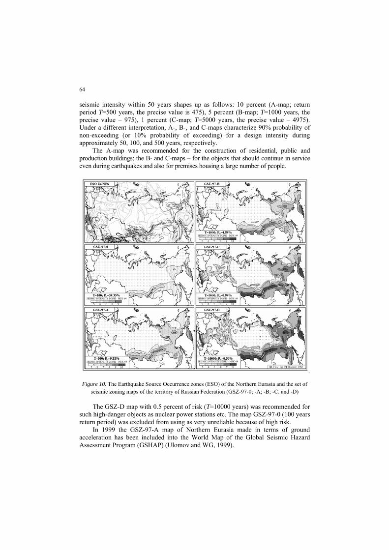
64

seismic intensity within 50 years shapes up as follows: 10 percent (A-map; return period T=500 years, the precise value is 475), 5 percent (B-map; T=1000 years, the precise value – 975), 1 percent (C-map; T=5000 years, the precise value – 4975). Under a different interpretation, A-, B-, and C-maps characterize 90% probability of non-exceeding (or 10% probability of exceeding) for a design intensity during approximately 50, 100, and 500 years, respectively.

The A-map was recommended for the construction of residential, public and production buildings; the B- and C-maps – for the objects that should continue in service even during earthquakes and also for premises housing a large number of people.

Figure 10. The Earthquake Source Occurrence zones (ESO) of the Northern Eurasia and the set of seismic zoning maps of the territory of Russian Federation (GSZ-97-0; -A; -B; -C. and -D) The GSZ-D map with 0.5 percent of risk (T=10000 years) was recommended for

such high-danger objects as nuclear power stations etc. The map GSZ-97-0 (100 years return period) was excluded from using as very unreliable because of high risk.

In 1999 the GSZ-97-A map of Northern Eurasia made in terms of ground acceleration has been included into the World Map of the Global Seismic Hazard Assessment Program (GSHAP) (Ulomov and WG, 1999).

65

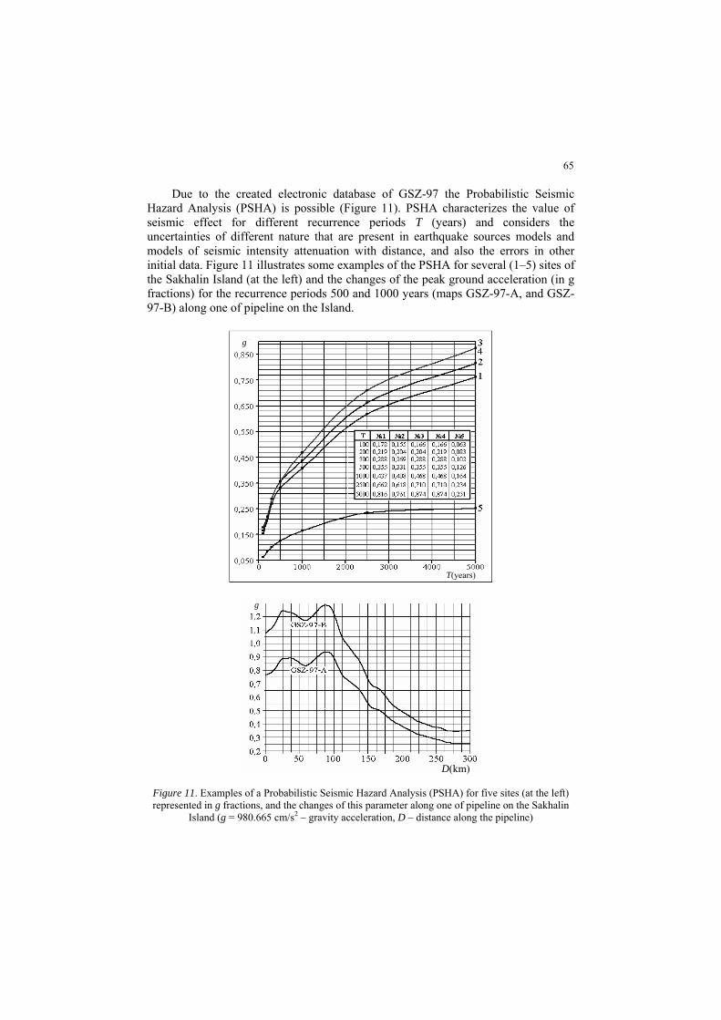
Due to the created electronic database of GSZ-97 the Probabilistic Seismic Hazard Analysis (PSHA) is possible (Figure 11). PSHA characterizes the value of seismic effect for different recurrence periods T (years) and considers the uncertainties of different nature that are present in earthquake sources models and models of seismic intensity attenuation with distance, and also the errors in other initial data. Figure 11 illustrates some examples of the PSHA for several (1–5) sites of the Sakhalin Island (at the left) and the changes of the peak ground acceleration (in g fractions) for the recurrence periods 500 and 1000 years (maps GSZ-97-A, and GSZ-97-B) along one of pipeline on the Island.

Figure 11. Examples of a Probabilistic Seismic Hazard Analysis (PSHA) for five sites (at the left) represented in g fractions, and the changes of this parameter along one of pipeline on the Sakhalin

Island (g = 980.665 сm/s2 – gravity acceleration, D – distance along the pipeline)

D(km)

T(years)

g

g

66

5. Conclusions

The new study of seismogeodynamics and seismic zoning is based on the new methodology, homogeneous data base compiled for Northern Eurasia, and the 3-D lineament-domain-focal (LDF) model of earthquake sources. The set of new General Seismic Zoning Maps (GSZ-97) has been accepted as the basis for the national Building Code.

As have shown results of our researches the territory of Russian Federation it is subjected to higher seismic danger, than it was represented before. About one third the area of the country is occupied by very high hazard zones of seismic intensity 8, 9, and 10 (MSK-64 – EMS-98 scales). These include the Russian Far East, the entire southern Siberia and Northern Caucasus. Some threat is also posed by intensity 6～7 zones in European Russia.

In this connection the Government of Russian Federation has ratified the Federal Program “Seismic safety of territory of Russia” (2002～2010). Up to this time neither in the former USSR, nor in Russia similar programs exist. The purpose of this Program is the maximal increase of seismic safety of the population, reduction of social, economic, ecological risk in seismically dangerous areas of the Russian Federation, decrease of damages from destructive earthquakes by certification, strengthening and reconstruction of existing buildings and constructions, and also preparation of cities and other settlements, transport, power constructions, pipelines for strong earthquakes.

Acknowledgements This work was supported by the Federal Research Program of Russia “Global Changes of Environment and Climate”. The author wish to thank the nearest colleagues accepting active participation in these researches, and first of all A. A. Gusev, N. V. Kondorskaya, L. S. Shumilina and V. G. Trifonov.

References Aptikaev, F. F. and Shebalin, N. V., 1988. Improvement of correlations between the level of

macroseismic effect and dynamical parameters of the ground motion. Investigations on seismic hazard. Problems of Eng. Seism. Hazard 29, Moscow, 98-107.

Arias, A., 1970. A measure of seismic intensity. Seismic Design for Nuclear Power Plants, M.I.T. Press, Cambridge, 438-483.

Cornell, C. A., 1968. Engineering seismic risk analysis. Bull. Seism. Soc. Amer. 58, 1583-1906. Gamburtsev, G. A., 1955. State and perspectives of work in the area of earthquake prediction, Bull.

Sov. of Seismol. 1 (in Russian). Golitsyn, B. B., 1912. New organization of seismic service in Russia, Izvestiya Post. Seism. Comis.

Imperial Acad. Sci. , St.-Peterburg (in Russian). Gusev, A. A., 1984. A descriptive statistical model for radiation of the earthquake source and its

application to the assessment of strong ground motion. Volc. and Seismol. 1, 3-22 (in Russian). Gusev, A. A., Pavlov, V. M. and Shumilina, L. S., 1998. A new approach to recurrence of

earthquake excitation for constructing seismic zoning maps. Proc. Conf. RAN on Problems Faced by the International Disaster Reduction Decade, Moscow, 7-9 October 1998, 26 (in Russian).

67

Gusev, A. A. and Shumilina, L. S., 2000. Modeling the intensity-magnitude-distance relation based on the concept of an incoherent extended earthquake source. Volc. and Seismol. 21, 443-463.

Gubin, I. E., 1950. The seismotectonic method of seismic zonation. Trudy Geofiz. Instituta AN SSSR, 13(140) (in Russian).

Medvedev, S. V., 1947. On the problem of taking into account the seismic activity of a region during construction. Trudy Seismol. Inst. AN SSSR, 119 (in Russian).

Mushketov, I. V. and Orlov A.N., 1893. Catalogue of earthquakes in the Russian Empire. St.-Petersburge. 307 (in Russian).

Riznichenko, Yu. V., 1965. From the activity of seismic sources to the intensity recurrence at the ground surface. Izv. AN SSSR, Fizika Zemli. 11, 1-12, (in Russian).

Schwartz, D. E. and Coppersmith, K. J., 1984. Fault behavior and characteristic earthquakes: examples from the Wasatch and San Andreas Fault Zones. J. Geophys. Res. 89, 5681-5698.

Shapira, A., 1983. A probabilistic approach for evaluating earthquake risk, with application to the Afro-Eurasian junction. Tectonophysics 91, 321-334.

Ulomov,V. I., 1974. Dynamics of the Earth's Crust in Central Asia and Earthquake Prediction. FAN, Tashkent, Uzbekistan (in Russian).

Ulomov, V. I., 1987. Lattice model of source seismicity and seismic hazard prediction. Uzbek Geolog. Journ. 6, 20-25 (in Russian).

Ulomov, V. I., 1993a. Global regularity of seismogeodynamic structures and some aspects of seismic zoning and long-term earthquakes prediction. Ulomov, V. I. (Ed.), Seismicity and Seismic Zoning of Northern Eurasia, Moscow, Russia, 24–44 (in Russian).

Ulomov, V. I., 1993b. Waves of seismogeodynamic activation and long-term earthquake prediction. Physics of the Earth. 4, 43-53 (in Russian).

Ulomov, V. I., 1994. Structural and dynamical regularity of Eurasia seismicity and some aspects of seismic hazard prediction. Proc. XXIV Gen. Ass. ESC, Vol. 1. Athens, Greece, 271-281.

Ulomov, V. I., 1997. On the identification and seismological parameterization of earthquake source zones. The Caucasus and adjacent area. Giardini, D. and Balassanian, S. (Eds.), Historical and Prehistorical Earthquakes in the Caucasus. NATO ASI. Ser. 2: Environ. 28, ILP Pub. 333, Kluwer Academic Publishers, Dordrecht, 503-522.

Ulomov, V. I., 1998. Modeling of zones of earthquake source origination on the basis of lattice regularization. Phys. of the Earth. 9, 1-20 (in Russian).

Ulomov, V. I., 2000. Seismogeodynamics and seismic mapping of North Eurasia. Volc. and Seismol. 21, 407-432.

Ulomov, V. I., 2002. Seismic zoning. Kotliakov, V. (Ed.), Natural Disasters. Encyclopedia of Life Support Systems. Earth and Atmospheric Sciences. Vol. I, EOLSS Publishers Co. Ltd. Oxford, 181-207.

Ulomov, V. I. and Shumilina, L. S., 1999. Set of General Seismic Zoning Maps of the Russian Federation. Scale 1:8,000,000. Explanatory Note. Moscow (in Russian).

Ulomov, V. I., Shumilina, L., Trifonov, V., Kronrod, T., Levi, K., Zhalkovsky, N., Imaev, V., Ivatschenko, A., Smirnov, V., Gusev, A., Balassanian, S., Gassanov, A., Ayzberg, R., Chelidze, T., Kurskeev, A., Tudukulov, A., Drumya, A., Negmatullaev, S., Ashirov, T., Pustovitenko, B. and Abdullabekov, K., 1999. Seismic hazard of northern Eurasia. Annali Geofis. 42, 1023-1038.

Wesnousky, S. G., 1990. Seismicity as a function of cumulative geologic offset: Some observations from southern California. Bull. Seism. Soc. Amer. 80, 1374-1381.

Wesnousky, S. G., Scholz, C. H., Shimazaki, K. and Matsuda, T., 1984. Integration of geological and seismological data for the analysis of seismic hazard; a case study of Japan. Bull. Seism. Soc. Amer. 74, 687-708.

Youngs, R. R. and Coppersmith, K. J., 1985. Implications of fault slip rates and earthquake recurrence models to probabilistic seismic hazard estimates. Bull. Seism. Soc. Amer. 75, 939-964.