research on the collision avoidance algorithm for fixed

applied sciences

Article

Research on the Collision Avoidance Algorithm forFixed-Wing UAVs Based on Maneuver Coordinationand Planned Trajectories Prediction

Yu Wan , Jun Tang * and Songyang Lao *

College of systems engineering, National University of Defense Technology, Changsha 410073, China;[email protected]* Correspondence: [email protected] (J.T.); [email protected] (S.L.)

Received: 15 January 2019; Accepted: 21 February 2019; Published: 25 February 2019��

Abstract: This paper presents a novel collision avoidance (CA) algorithm for a cooperative fixed-wingunmanned aerial vehicle (UAV). The method is based on maneuver coordination and plannedtrajectory prediction. Each aircraft in a conflict generates three available maneuvers and predictsthe corresponding planned trajectories. The algorithm coordinates planned trajectories betweenparticipants in a conflict, determines which combination of planned trajectories provides the bestseparation, eventually makes an agreement on the maneuver for collision avoidance and activates thepreferred maneuvers when a collision is imminent. The emphasis is placed on providing protectionfor UAVs, while activating maneuvers late enough to reduce interference, which is necessary forcollision avoidance in the formation and clustering of UAVs. The CA has been validated withvarious simulations to show the advantage of collision avoidance for continuous conflicts in multiple,high-dynamic, high-density and three-dimensional (3D) environments. It eliminates the disadvantageof traditional CA, which has high uncertainty, and takes the performance parameters of differentaircraft into consideration and makes full use of the maneuverability of fixed-wing aircraft.

Keywords: fixed-wing UAV; Collision avoidance; conflict resolution; maneuver coordination

1. Introduction

There are many studies in collision avoidance that could be sorted out into two main domains,i.e., tactical and strategic [1]. The first is the geometric algorithm, which analyzes the relative motionof aircraft in geometric space and implements passive collision avoidance under the procedureof detection-avoidance [2–5]. The other is the track planning algorithm, which actively plans theconflict-free flight path from the current position to the destination based on the perception detectionof obstacles under the constraint of minimum safety separation distance. The geometric algorithm iswidely researched. Chakravarthy A [3] and Carbone C [4] proposed a novel collision cone approachfor irregularly shaped moving objects with unknown trajectories. Luongo S [5] improved the3D analytical algorithm by proposing a cylindrical safety bubble that allows different minimumseparations of the vertical and horizontal planes with respect to the nominal trajectory to be achieved.The performances of such system, using active obstacle detection through radar, have been discussedin the paper [6]. Geometric algorithm is intuitive with low computing cost and always providesan optimal solution in 3D environments whether the aircraft cooperates or not. But most of thecurrent Genetic Algorithm (GA) only focus on pairwise encounters. For multiple conflict resolution,more complicated algorithm should be considerable, the calculation amount of checking each threatrepeatedly becomes inconsiderably massive. Smith A L [7] presented an aggregate collision coneapproach to allow aircrafts to detect and avoid collisions with more threats simultaneously. But there

Appl. Sci. 2019, 9, 798; doi:10.3390/app9040798 www.mdpi.com/journal/applsci

http://www.mdpi.com/journal/applsci

http://www.mdpi.com

https://orcid.org/0000-0002-0336-8658

http://www.mdpi.com/2076-3417/9/4/798?type=check_update&version=1

http://dx.doi.org/10.3390/app9040798

http://www.mdpi.com/journal/applsci

Appl. Sci. 2019, 9, 798 2 of 20

are only three aircrafts in experiments [8]. The geometric algorithm to be used, furthermore, is alsodependent, to some extent, from the available sensors onboard, as emphasized in the paper [9].

The main aspects of the track planning algorithm include the potential field method [10–12],linear programming, discretized space domain and stochastic theory methods, and so on. Liu J Y [11]improved the artificial potential field by combining the Lyapunov theorem to make the disturbingbalance points divergent so that the Unmanned Aerial Vehicle (UAV) can avoid the minimum point.Ruchti J [12] modified the artificial potential fields by combining a priority system to prevent thespecial case of an aircraft circling its destination. The artificial potential field has the advantage of rapidrespondent speed, small computation capacity and real-time property. However, there exist someproblems, such as the unreachable goal and the existence of a local minimum point value, and these donot apply to the fixed-wing aircraft due to continuous adjustment and an unstable state [13]. To planan optimal trajectory for collision avoidance, Xiaohua X [14] developed an algorithm of modifiedGrossberg neural network (GNN) to get the trajectories outside of the danger zone based on currentsensor information and mission objectives. GNN has been used earlier in robot applications andis implementable in UAVs that have limited capabilities. Cheng P [15] developed an algorithm ofrapidly exploring random trees (RRT), Y. Kuwata [16] proposed an algorithm of mixed integer linearprogramming (MILP), and Cekmez U [17], Nikolos I K [18], Yao X [19] applied ant colony optimizationalgorithm (ACO). These algorithms have obvious defects of limited application; they apply mostlyto an immovable obstacle and cannot solve a dynamic obstacle. In addition, they require massiveiterative calculation, which suits of-line route planning but not real-time planning.

To solve the multi-aircraft conflict, Manathara J G [20] proposed a consensus algorithm to solvethe rendezvous problem by attaining a consensus on the estimated time of arrivals. However, it couldnot manage dynamic obstacles. Archibald [21] proposed a satisficing decision theory by applyingthe game theory, but it lacks efficiency and suits a 2D model of airspace. George J [22] developed areactive inverse proportional navigation (PN) algorithm by increasing Line of Slight (LOS) rate, but thealgorithm is inefficient and defective in some scenarios. Sharma R K [23] applied swarm intelligencetechniques to collision avoidance between UAVs. Turner R [24] Ikeda Y [25] Wadley J [26] introducedan automatic air collision avoidance system (Auto ACAS) that coordinates maneuver trajectoriesbetween fighters. Although Auto-ACAS applies to fighters, it provides a good concept for the collisionavoidance of fixed-wing UAVs.

Traffic Collision Avoidance System (TCAS) is designed as the final safeguard to resolve midaircollisions (MACs) and evidently decrease near midair collisions (NMACs) in the aviation densities ofup to 24 aviation vehicles within a 5NM radius [27]. There is great difference between the proposedmethodology and the TCAS. Firstly, TCAS only suggests maneuvers in vertical direction to the pilot,while the proposed methodology includes automatic maneuver implementation in all directions.Secondly, The TCAS performs well in solving one-on-one threats between traditional aircrafts, but insome complex situations, TCAS would issue improper maneuvers while a new secondary encounteris induced to the nearby (remotely piloted aircraft) RPA of previous operations [28]. While theproposed methodology is designed for multiple threats in formation and clusters. The coordinationof maneuvers is among all participants in a conflict. Thirdly, the logics are quite different. In TCAS,an RA is produced in real time, the direction choosing and change of vertical speed depends on thecurrent relative situation, while in proposed methodology, the maneuver style (MS) is pre-set to agroup of specific categories, the aircrafts choose from the specified maneuver styles.

Aiming to solve the defects of traditional CA, this paper presents a novel collision avoidancealgorithm for fixed-wing UAVs based on maneuver coordination and planned trajectory prediction,which takes full advantage of the maneuverability of fixed-wing UAVs and generates the collisionavoidance maneuver based on the coordination of planned trajectories. The proposed algorithmis classified as the mixed style, which has features that refer to both tactical and strategic domainsaddressed in the literature analysis. When solving collision, the proposed algorithm plans collision-freesafety routes (planned trajectories) for UAVs, and in module of maneuver evaluation and maneuver

Appl. Sci. 2019, 9, 798 3 of 20

activation, it draws lessons from methods of Point of closed Approach (PCA), and Collision ConeApproach (CCA).

This paper is organized as follows: Section 2 summarizes the operational principle; Section 3describes the module of maneuver generation and presents the module of trajectory prediction;Section 4 presents the module of treat management; Section 5 presents the module of maneuverevaluation; Section 6 presents the module of maneuver activation; Section 7 presents a couple ofscenario simulations and their results; Finally, the conclusions and future work are summarized inSection 8.

2. Operational Principle

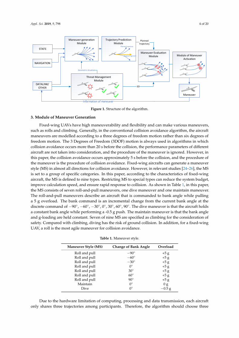
Among fixed-wing UAVs in a conflict, which are called participants, the algorithm coordinatesavailable maneuvers, generates and shares responding planned trajectories, decides the combinationof planned trajectories to provide the best separation, and activates the preferred maneuvers when acollision is extremely imminent. The structure of the algorithm is shown in Figure 1. Based on the hostcondition, navigation solution, radar target location, data link and other information, each host aircraftdetermines the severity of the risk posed by the threat aircraft. Through a special datalink, UAVsthat are participants in a conflict communicate with each other. According to the relative positionand motion between participants, each participant chooses three maneuvers from a pool of nineavailable maneuvers that may be performed to avoid collision. Three trajectories responding to thethree maneuvers are generated through the trajectory prediction module and then are shared amongthe participants via a data link. The evaluation module compares the combinations of the plannedtrajectories and determines the optimal combination of maneuvers with the maximal separation. In theoptimal combination of maneuvers, each participant has a preferred maneuver. The system updatesand repeats the above procedure, thus generating new maneuvers and evaluating a combination ofmaneuvers at regular intervals. Meanwhile, the system will activate the preferred maneuver when theplanned trajectories converge in time and space.

The five modules of the algorithm are as follows:

1. Module of maneuver generation: the module chooses three maneuvers from a pre-set pool ofnine available maneuvers according to the relative situation and motion between the host aircraftand threats.

2. Module of trajectory prediction: the module predicts the three planned trajectories respondingto the three maneuvers. The trajectories are predicted based upon the current status andcontrol parameters.

3. Module of threat management: the module of threat management determines if a UAV poses athreat to the host aircraft and evaluates the risk degree of threats.

4. Module of maneuver evaluation: the module evaluates combinations of three planned trajectoriesof each participant and determines which combination can delay the activation of the maneuveras far as possible. Through the maneuver evaluation, the three maneuvers are tagged as onepreferred maneuver and two alternative maneuvers separately. Once tagged, the determinationis shared among each participant

5. Module of maneuver activation: the module judged whether the planned trajectories ofparticipants will converge in time and space. If so, the preferred maneuver is activated, and theaircraft will maneuver to avoid collision.

Appl. Sci. 2019, 9, 798 4 of 20

Appl. Sci. 2019, 9, x 4 of 20

STATE

NAVIGATION

DATALINK/OTHER

Maneuver generation Module

Maneuver Evaluation Module

3D

Information of maneuver

Module of Maneuver Activation

Trajectory Predictiion Module

Geometric situation

Original trajectory

Threat Management Module

Planned trajectory

Maneuver

Figure 1. Structure of the algorithm.

3. Module of Maneuver Generation

Fixed-wing UAVs have high maneuverability and flexibility and can make various maneuvers, such as rolls and climbing. Generally, in the conventional collision avoidance algorithm, the aircraft maneuvers are modelled according to a three degrees of freedom motion rather than six degrees of freedom motion. The 3 Degrees of Freedom (3DOF) motion is always used in algorithms in which collision avoidance occurs more than 20 s before the collision, the performance parameters of different aircraft are not taken into consideration, and the procedure of the maneuver is ignored. However, in this paper, the collision avoidance occurs approximately 5 s before the collision, and the procedure of the maneuver is the procedure of collision avoidance. Fixed-wing aircrafts can generate a maneuver style (MS) in almost all directions for collision avoidance. However, in relevant studies [24–26], the MS is set to a group of specific categories. In this paper, according to the characteristics of fixed-wing aircraft, the MS is defined to nine types. Restricting MS to special types can reduce the system budget, improve calculation speed, and ensure rapid response to collision. As shown in Table 1, in this paper, the MS consists of seven roll-and-pull maneuvers, one dive maneuver and one maintain maneuver. The roll-and-pull maneuvers describe an aircraft that is commanded to bank angle while pulling a 5 g overload. The bank command is an incremental change from the current bank angle at the discrete command of -90°, -60°, -30°, 0°, 30°, 60°, 90°. The dive maneuver is that the aircraft holds a constant bank angle while performing a -0.5 g push. The maintain maneuver is that the bank angle and g-loading are held constant. Seven of nine MS are specified as climbing for the consideration of safety. Compared with climbing, diving has the risk of ground collision. In addition, for a fixed-wing UAV, a roll is the most agile maneuver for collision avoidance.

Table 1. Maneuver style.

Maneuver Style (MS) Change of Bank Angle Overload Roll and pull −90° +5 g Roll and pull −60° +5 g Roll and pull −30° +5 g Roll and pull 0° +5 g Roll and pull 30° +5 g Roll and pull 60° +5 g Roll and pull 90° +5 g

Maintain 0° 0 g Dive 0° −0.5 g

Due to the hardware limitation of computing, processing and data transmission, each aircraft only shares three trajectories among participants. Therefore, the algorithm should choose three available maneuvers from the nine maneuvers first. The procedure of preselection does not need

Figure 1. Structure of the algorithm.

3. Module of Maneuver Generation

Fixed-wing UAVs have high maneuverability and flexibility and can make various maneuvers,such as rolls and climbing. Generally, in the conventional collision avoidance algorithm, the aircraftmaneuvers are modelled according to a three degrees of freedom motion rather than six degrees offreedom motion. The 3 Degrees of Freedom (3DOF) motion is always used in algorithms in whichcollision avoidance occurs more than 20 s before the collision, the performance parameters of differentaircraft are not taken into consideration, and the procedure of the maneuver is ignored. However, inthis paper, the collision avoidance occurs approximately 5 s before the collision, and the procedure ofthe maneuver is the procedure of collision avoidance. Fixed-wing aircrafts can generate a maneuverstyle (MS) in almost all directions for collision avoidance. However, in relevant studies [24–26], the MSis set to a group of specific categories. In this paper, according to the characteristics of fixed-wingaircraft, the MS is defined to nine types. Restricting MS to special types can reduce the system budget,improve calculation speed, and ensure rapid response to collision. As shown in Table 1, in this paper,the MS consists of seven roll-and-pull maneuvers, one dive maneuver and one maintain maneuver.The roll-and-pull maneuvers describe an aircraft that is commanded to bank angle while pullinga 5 g overload. The bank command is an incremental change from the current bank angle at thediscrete command of −90◦, −60◦, −30◦, 0◦, 30◦, 60◦, 90◦. The dive maneuver is that the aircraft holdsa constant bank angle while performing a -0.5 g push. The maintain maneuver is that the bank angleand g-loading are held constant. Seven of nine MS are specified as climbing for the consideration ofsafety. Compared with climbing, diving has the risk of ground collision. In addition, for a fixed-wingUAV, a roll is the most agile maneuver for collision avoidance.

Table 1. Maneuver style.

Maneuver Style (MS) Change of Bank Angle Overload

Roll and pull −90◦ +5 gRoll and pull −60◦ +5 gRoll and pull −30◦ +5 gRoll and pull 0◦ +5 gRoll and pull 30◦ +5 gRoll and pull 60◦ +5 gRoll and pull 90◦ +5 g

Maintain 0◦ 0 gDive 0◦ −0.5 g

Due to the hardware limitation of computing, processing and data transmission, each aircraftonly shares three trajectories among participants. Therefore, the algorithm should choose three

Appl. Sci. 2019, 9, 798 5 of 20

available maneuvers from the nine maneuvers first. The procedure of preselection does not needdata-transportation among participants and is only based on the geometric relations and motionrelations between the host aircraft and threats, including those that are forward or backward, above orbelow, or on the left or right side of the aircraft.

4. Module of Trajectory Prediction

The module of trajectory prediction generates the future trajectory based on state and controlparameters using the six-degrees-of-freedom simulation. Three planned trajectories correspondingto three maneuvers are generated and are shared among participants. According to the principle ofnoninterference, activation of the maneuver often occurs three to four seconds before the collision,and most maneuvers last only two to three seconds. Therefore, the forecast time is required to exceed4 s, but long forecast time will prominently increase the amount of computation. Comprehensivelyconsidering the collision avoidance effect and the operation cost, the forecast duration in this paperis set to 5 s, and the module generates the future planned trajectories from the present to 5 s later.As shown in Figure 2, the planned trajectory is a conical region whose size depends on the uncertaintyover time. Considering the factors such as accuracy, efficiency and the performance of UAVs providedby our team comprehensively, the frequency of this module is set to 10 Hz. The predicted trajectoryconsists of 50 discrete positions. As is shown in the figure, the planned trajectory is a conical regionCR(t, t + ∆t), ∆t ∈ (0, T), the midline of it is the predicted trajectory constructed by 50 predictivepositions P(t + ∆t), and the cross-section size represents the error radius UD(∆t), which dependson the uncertainty of the trajectory prediction and increases over time ∆t. The set of error radiusis to ensure that most of the actual predicted trajectories fall within the conical region. The errorradius is relevant with uncertainties including navigation uncertainty, trajectory prediction uncertainty,trajectory reconstruction uncertainty, data link transmission uncertainty, and uncertainty in track datacomputation. The error radius UD(∆t) is the quadratic function of time: UD(∆t) = a.(∆t)2 + b.∆t.The index of a and b is relevant with types of aircraft, equipment and environment. They can beobtained by actual experiment through comparing the predicted trajectories with the real trajectories.Considering UAVs provided by our team and the performance of experiments, the value of a is 0.425,the value of b is 1.19. The model of conical region is as follows:

∀CR(t + ∆t) ⊆ (P(t + ∆t)−UD(∆t) P(t + ∆t) + UD(∆t)), ∆t ∈ (0, T) (1)

Appl. Sci. 2019, 9, x 5 of 20

data-transportation among participants and is only based on the geometric relations and motion relations between the host aircraft and threats, including those that are forward or backward, above or below, or on the left or right side of the aircraft.

4. Module of Trajectory Prediction

The module of trajectory prediction generates the future trajectory based on state and control parameters using the six-degrees-of-freedom simulation. Three planned trajectories corresponding to three maneuvers are generated and are shared among participants. According to the principle of noninterference, activation of the maneuver often occurs three to four seconds before the collision, and most maneuvers last only two to three seconds. Therefore, the forecast time is required to exceed 4 s, but long forecast time will prominently increase the amount of computation. Comprehensively considering the collision avoidance effect and the operation cost, the forecast duration in this paper is set to 5 s, and the module generates the future planned trajectories from the present to 5 s later. As shown in Figure 2, the planned trajectory is a conical region whose size depends on the uncertainty over time. Considering the factors such as accuracy, efficiency and the performance of UAVs provided by our team comprehensively, the frequency of this module is set to 10 Hz. The predicted trajectory consists of 50 discrete positions. As is shown in the figure, the planned trajectory is a conical region CR 𝑡, 𝑡 + ∆𝑡 , ∆𝑡 ∈ 0, 𝑇 , the midline of it is the predicted trajectory constructed by 50 predictive positions P 𝑡 + ∆𝑡 , and the cross-section size represents the error radius UD ∆𝑡 , which depends on the uncertainty of the trajectory prediction and increases over time ∆𝑡. The set of error radius is to ensure that most of the actual predicted trajectories fall within the conical region. The error radius is relevant with uncertainties including navigation uncertainty, trajectory prediction uncertainty, trajectory reconstruction uncertainty, data link transmission uncertainty, and uncertainty in track data computation. The error radius UD ∆𝑡 is the quadratic function of time: UD ∆𝑡 = 𝑎. ∆𝑡 + 𝑏. ∆𝑡. The index of a and b is relevant with types of aircraft, equipment and environment. They can be obtained by actual experiment through comparing the predicted trajectories with the real trajectories. Considering UAVs provided by our team and the performance of experiments, the value of a is 0.425, the value of b is 1.19. The model of conical region is as follows: ∀CR 𝑡 + ∆𝑡 ⊆ P 𝑡 + ∆𝑡 − UD ∆𝑡 P 𝑡 + ∆𝑡 + UD ∆𝑡 , ∆𝑡 ∈ 0, 𝑇 (1)

Predicted Position P(t+Δt)

UD（Δt）

Predicted Trajectory

Starting Position P(t)

CR(t,t+Δt)

Figure 2. Planned trajectories.

The module of trajectory prediction is based on the six-degrees-of-freedom aircraft model. According to standard build-up method using dimensionless coefficients, we establish and approximate force and moments. [29]

5. Module of Threat Management

During the encounter of clusters of UAVs, a UAV might be threatened by multiple aircraft. However, due to the hardware limitation of computing, processing and data transmission, it is

Figure 2. Planned trajectories.

The module of trajectory prediction is based on the six-degrees-of-freedom aircraft model.According to standard build-up method using dimensionless coefficients, we establish andapproximate force and moments [29].

Appl. Sci. 2019, 9, 798 6 of 20

5. Module of Threat Management

During the encounter of clusters of UAVs, a UAV might be threatened by multiple aircraft.However, due to the hardware limitation of computing, processing and data transmission, it isimpossible for the host UAV to respond to all threats by UAVs at the same time. The system onlyconcentrates on the three most imminent threats. The module of threat management monitors eachsurrounding aircraft and scores each of the threats to decide the three greatest threats. The systemupdates the threats at regular times, which is the same as the cycle in the module of trajectory prediction.Through the procedure, the module reduces the full threat list to a shorter list of the most at-riskaircraft which is defined as threats.

The risk degree (R) is determined by a weighted combination of the relative distance (RD) andthe relative speed (RS). The risk range between aircraft A and T is as follows.

R =RSRD

, RS > 0 (2)

RD =

√(uA − uT)

2 + (vA − vT)2 + (wA −wT)

2 (3)

RS =(xT − xA)× (uT − uA) + (yT − yA)× (vT − vA) + (zT − zA)× (wT − wA)√

(xT − xA)2 + (yT − yA)

2 + (zT − zA)2

(4)

When aircraft are separating, the relative speed is negative, and it is eliminated from the scoringequation. When aircrafts are approaching, the relative speed is positive, and higher relative speedmeans higher approaching speed. After scoring, the threats are often sorted based on the score, higherdegree means higher risk. The threats with the three highest scores are selected as participants forprocessing in the module of maneuver generation and in the module of maneuver evaluation.

6. Module of Maneuver Evaluation

At each run step, the system chooses three maneuvers and generates the corresponding plannedtrajectories. The trajectories are shared among participants to reach an agreement on a combination ofmaneuvers that supply the best solution. Each aircraft receives the planned trajectories via a datalinkfrom the other participants, scores the combinations independently and selects the best maneuver fromthe three maneuvers as the preferred maneuver. Although the system predicts which maneuver eachthreat aircraft should perform, the system only selects a maneuver for its own aircraft. Thus, to reachconsistent decisions among participants, the module of maneuver evaluation should utilize nearlyidentical information available to participants. Before performing a maneuver, the system requests across check to ensure consistency in maneuver evaluation.

Then, the labeled trajectories are shared among the participants via a datalink to keep insynchronization and coherence. There would be nine combinations of maneuvers for two participants,and 81 combinations of maneuvers for four participants. The frequency is set at 4 Hz, so the moduleshares planned trajectories and evaluates the combination of maneuvers every 0.25 s. However, in theactual situation, the transmission latency is unavoidable in data sharing, the maneuvers will becomeuncoordinated and the system will be mispositioned if the algorithm attempts the process too rapidly.

To solve this problem, two measures were taken in this module. First, in the algorithm,the frequency of the different modules was set differently, the frequency of the maneuver generatingmodule and the trajectory prediction module were set at 10 Hz, which was higher than that of maneuverevaluation. There is adequate time for aircraft to wait and receive data from other participants. Even aloss or delay of data will not affect the evaluation. When the algorithm evaluates a combination ofmaneuvers at one run step, the data are ready for the previous step. Second, considering the continuityand stability of the relative situation between participants in continuous frames of time, the maneuverswill last from the last time frame to the next. In the procedure of maneuver generation, the preferredmaneuver in the last time frame remains one of the three newly generated maneuvers.

Appl. Sci. 2019, 9, 798 7 of 20

The principle of evaluating the optimal combination of maneuvers is to select the one that candelay the activation of maneuvers as much as possible. The system chooses the combination with thesmallest cost. The cost function is the sum of reciprocal predicted minimum avoidance distance (PAD).The predicted minimum avoidance distance (PAD) is the minimum distance between a conical regionin the space-time domain, which is the distance of the predicted trajectory subtracting the uncertaintydistance (UD). As is illustrated in Figure 3, there are nine possible combinations of maneuvers amongthe two participants, but the combination of planned trajectory A and b provides the maximum PAD.

∀∆t ∈ (0, T), PAD(

Mi(m), Mj(n))= min

(∣∣Pi(t + ∆t)− Pj(t + ∆t)∣∣−UDi(∆t)−UDj(∆t)

)(5)

ωij(m, n) = PAD(

Mi(m), Mj(n))

(6)

Indeed, Mi(m) represents that aircraft i takes maneuver m; PAD(

Mi(m), Mj(n))

represents PAD whenaircraft i takes maneuver m, aircraft j takes maneuver n.

The cost function is as follows:

cos t(

Mi(m), Mj(n), . . . . . . ,)= min

N

∑i=1

N

∑j=1

ωij (7)

Indeed, i 6= j, m = 1, 2, 3, n = 1, 2, 3.The maneuvers that aircraft should take:

ACT(

Mi(k), Mj(k), . . . . . . ,)= argmin

N

∑i=1

N

∑j=1

ωij (8)

Indeed i 6= j

Appl. Sci. 2019, 9, x 7 of 20

conical region in the space-time domain, which is the distance of the predicted trajectory subtracting the uncertainty distance (UD). As is illustrated in Figure 3, there are nine possible combinations of maneuvers among the two participants, but the combination of planned trajectory A and b provides the maximum PAD. ∀∆𝑡 ∈ 0, 𝑇 , 𝑃𝐴𝐷 𝑀 𝑚 ,𝑀 𝑛 = 𝑚𝑖𝑛 𝑃 𝑡 + ∆𝑡 − 𝑃 𝑡 + ∆𝑡 − UD ∆𝑡 -UD ∆𝑡 (5) 𝜔 𝑚, 𝑛 = 𝑃𝐴𝐷 𝑀𝑖 𝑚 ,𝑀𝑗 𝑛 (6)

Indeed,𝑀 𝑚 represents that aircraft i takes maneuver m ;𝑃𝐴𝐷 𝑀 𝑚 ,𝑀 𝑛 represents PAD when aircraft i takes maneuver m, aircraft j takes maneuver n.

The cost function is as follows:

𝑐𝑜𝑠 𝑡 𝑀 𝑚 ,𝑀 𝑛 ,…… , = 𝑚𝑖𝑛 𝜔 (7)

Indeed,𝑖 ≠ 𝑗, m = 1, 2, 3, n = 1, 2, 3 The maneuvers that aircraft should take:

𝐴𝐶𝑇 𝑀 𝑘 ,𝑀 𝑘 ,…… , = 𝑎𝑟𝑔𝑚𝑖𝑛 𝜔 (8)

Indeed 𝑖 ≠ 𝑗

Cone a

Cone c

Cone B

Cone bCone C

Cone A

Aircraft A

Aircraft B

PAD of Cone Cc

Figure 3. Maneuver evaluation.

7. Module of Maneuver Activation

The principle of the system is noninterference and minimizing interference while simultaneously achieving collision avoidance. To realize this principle, the system should activate the maneuver as late as possible. The Figure 4 is the relative motion of aircraft A and B; aircraft B is resting relatively, while aircraft A is moving toward B relatively. The isolation sphere is the safety separation zone for aircraft B. Before entering the isolation sphere, aircraft A can activate a maneuver to avoid collision. The earlier aircraft B maneuvers, the more available options aircraft B can choose, and the less likely a collision will occur. There exists a final moment when activation is too late; no matter what maneuver is taken under the restriction of performance; aircraft A cannot avoid entering the isolation sphere of aircraft B and the collision between two UAVs cannot be prevented. If UAV A activates maneuvers at point 1, no matter which maneuver is taken, it can avoid collision, but if the

Figure 3. Maneuver evaluation.

7. Module of Maneuver Activation

The principle of the system is noninterference and minimizing interference while simultaneouslyachieving collision avoidance. To realize this principle, the system should activate the maneuver aslate as possible. The Figure 4 is the relative motion of aircraft A and B; aircraft B is resting relatively,while aircraft A is moving toward B relatively. The isolation sphere is the safety separation zone foraircraft B. Before entering the isolation sphere, aircraft A can activate a maneuver to avoid collision.

Appl. Sci. 2019, 9, 798 8 of 20

The earlier aircraft B maneuvers, the more available options aircraft B can choose, and the less likely acollision will occur. There exists a final moment when activation is too late; no matter what maneuveris taken under the restriction of performance; aircraft A cannot avoid entering the isolation sphere ofaircraft B and the collision between two UAVs cannot be prevented. If UAV A activates maneuvers atpoint 1, no matter which maneuver is taken, it can avoid collision, but if the activation time is too early,it will seriously interfere with the normal flight of the UAV. If UAV A activates at point 3, no matterwhich maneuver UAV A takes, it cannot avoid collision with UAV B for the restriction of performance.At point 3, only one maneuver can avoid collision, the planned trajectory is tangent to the isolationspheres, and the special maneuver is the preferred maneuver for aircraft A. In summary, the momentat point 2 is the last moment when collision can be avoided and is the best moment that satisfies thenoninterference principle. The radius of the sphere can be modified to increase or decrease the earlywarning time.

Appl. Sci. 2019, 9, x 8 of 20

activation time is too early, it will seriously interfere with the normal flight of the UAV. If UAV A activates at point 3, no matter which maneuver UAV A takes, it cannot avoid collision with UAV B for the restriction of performance. At point 3, only one maneuver can avoid collision, the planned trajectory is tangent to the isolation spheres, and the special maneuver is the preferred maneuver for aircraft A. In summary, the moment at point 2 is the last moment when collision can be avoided and is the best moment that satisfies the noninterference principle. The radius of the sphere can be modified to increase or decrease the early warning time.

Isolation sphere

Point 1 Point 2 Point 3

Prefered Maneuver

Aircraft A

Aircraft B

Alternative Maneuver

Figure 4. The moment to activate the maneuver.

The module of maneuver activation calculates the minimum allowed separation distance (MASD), which is the sum of the wing span (WS) of two aircrafts, plus the desired separation distance (DSD). The predicted minimum range (PMR) is the minimum distance between the conical region. 𝑀𝐴𝑆𝐷 = 𝐷𝑆𝐷 + 𝑊𝑆 (9) 𝑀𝑅 = 𝑚𝑖𝑛 |𝑃 𝑡 + ∆𝑡 − 𝑃 𝑡 + ∆𝑡 | + 𝑈𝐷 ∆𝑡 + 𝑈𝐷 ∆𝑡 , ∆𝑡 ⊆ 0, 𝑇 (10) UD ∆𝑡 = 0.425 ∗ ∆𝑡 + 1.19 ∗ ∆𝑡 (11)

MASD

PMR

The primary maneuver

Figure 5. Diagram of maneuver activation.

In the module of the maneuver activation, only the planned trajectories corresponding to preferred maneuver are considered to determine the activation. As shown in Figure 5, as the risk of collision becomes more likely, the cones of the two aircraft will converge in time and space when the predicted minimum range (PMR) is less than the permitted minimum allowed separation distance (MASD); then the maneuver is activated, and the participants take the preferred maneuver, and the UAV will fly in the planned trajectory. Indeed, the desired separation distance (DSD) is a fixed value that is input by the system in advance.

8. Results


The module of maneuver activation calculates the minimum allowed separation distance (MASD),which is the sum of the wing span (WS) of two aircrafts, plus the desired separation distance (DSD).The predicted minimum range (PMR) is the minimum distance between the conical region.

MASD = DSD + ∑ WS (9)

MR = min(|PA(t + ∆t)− PB(t + ∆t)|+ UDA(∆t) + UDB(∆t)), ∆t ⊆ (0, T) (10)

UD(∆t) = 0.425 ∗ (∆t)2 + 1.19 ∗ ∆t (11)

Appl. Sci. 2019, 9, x 8 of 20

activation time is too early, it will seriously interfere with the normal flight of the UAV. If UAV A activates at point 3, no matter which maneuver UAV A takes, it cannot avoid collision with UAV B for the restriction of performance. At point 3, only one maneuver can avoid collision, the planned trajectory is tangent to the isolation spheres, and the special maneuver is the preferred maneuver for aircraft A. In summary, the moment at point 2 is the last moment when collision can be avoided and is the best moment that satisfies the noninterference principle. The radius of the sphere can be modified to increase or decrease the early warning time.

Isolation sphere

Point 1 Point 2 Point 3

Prefered Maneuver

Aircraft A

Aircraft B

Alternative Maneuver


The module of maneuver activation calculates the minimum allowed separation distance (MASD), which is the sum of the wing span (WS) of two aircrafts, plus the desired separation distance (DSD). The predicted minimum range (PMR) is the minimum distance between the conical region. 𝑀𝐴𝑆𝐷 = 𝐷𝑆𝐷 + 𝑊𝑆 (9) 𝑀𝑅 = 𝑚𝑖𝑛 |𝑃 𝑡 + ∆𝑡 − 𝑃 𝑡 + ∆𝑡 | + 𝑈𝐷 ∆𝑡 + 𝑈𝐷 ∆𝑡 , ∆𝑡 ⊆ 0, 𝑇 (10) UD ∆𝑡 = 0.425 ∗ ∆𝑡 + 1.19 ∗ ∆𝑡 (11)

MASD

PMR

The primary maneuver


In the module of the maneuver activation, only the planned trajectories corresponding to preferred maneuver are considered to determine the activation. As shown in Figure 5, as the risk of collision becomes more likely, the cones of the two aircraft will converge in time and space when the predicted minimum range (PMR) is less than the permitted minimum allowed separation distance (MASD); then the maneuver is activated, and the participants take the preferred maneuver, and the UAV will fly in the planned trajectory. Indeed, the desired separation distance (DSD) is a fixed value that is input by the system in advance.

8. Results


In the module of the maneuver activation, only the planned trajectories corresponding to preferredmaneuver are considered to determine the activation. As shown in Figure 5, as the risk of collisionbecomes more likely, the cones of the two aircraft will converge in time and space when the predicted

Appl. Sci. 2019, 9, 798 9 of 20

minimum range (PMR) is less than the permitted minimum allowed separation distance (MASD);then the maneuver is activated, and the participants take the preferred maneuver, and the UAV will flyin the planned trajectory. Indeed, the desired separation distance (DSD) is a fixed value that is inputby the system in advance.

8. Results

To verify the effectiveness of the algorithm that was proposed in this paper, a simulationexperiment is operated in a series of special collision scenarios. The principle of the constructedscenarios are as follows:

• Complexity: The encounter scenarios constructed are relatively complex, reaching the complexityof the actual situation.

• Typicality: The collision scenarios constructed are common in the actual situation.• Extensibility: Most of the actual collision can be combined by the constructed collision scenarios.

Based on the three principles, six encounter scenarios were constructed, including six two-aircraft-encounter scenarios, a four-aircraft-encounter scenario and an eight-aircraft-encounter scenario.

In this paper, the UAVs are provided by our team in college of aerospace science and technology,National University of Defense Technology. And the basic attributes of UAV are as follows in Table 2:

Table 2. Attribute list of Unmanned Aerial Vehicles (UAVs).

Type Size Type Size

Mass 4536 kg Zero-AoA Lift Coefficient 0.1095Roll Moment of Inertia 35926.5 kg·m2 Parasite Drag Coefficient 0.0255Pitch Moment of Inertia 33940.7 kg·m2 Side-force Coefficient −0.7162

Yaw Moment of Inertia 67085.5 kg·m2 Zero-AoA MomentCoefficient 0

North-high Product of Inertia 3418.17 kg·m2 Yaw Moment Coefficient 0.1194Mean Aerodynamic 2.14 m Rolling Moment Coefficient −0.0918

Wing Span 10.4 m Static Thrust 26243.2 NSafe Distance 60 m

The safe distance is the minimum allowed distance between aircraft. Several factors need to beconsidered in the setting of safe distance. The safe distance must ensure that the isolation spheres oftwo aircraft would not touch each other. In other words, the safe distance must be greater than thesum of the two minimum allowed separation distances (MASD), which is the sum of the wing span(WS) (10.4 m) and the desired separation distance (DSD). The delay of distance calculation is also takeninto consideration, and the frequency of the module of trajectory prediction is set to 10 Hz, so theremight be a delay of 0.1s. The speed of UAV is less than 100m/s, so the error in distance is less than10 m. In summary, 10.4 × 2 + 10 × 2 = 40.8 (m). With DSD added, the safe distance is set to 60 m. Butthe safe distance is not fixed, the desired separation distance (DSD) can be adjusted to meet differentsecurity requirements. The smaller safe distance, the later the aircraft activates collision avoidancemaneuver. In Eight-aircraft-formation scenario, consider the high density of aircraft, we adjust the safedistance to 42 m.

8.1. Rear-Ended Scenario

There are two UAVs cruising at the same altitude in a certain airspace. The two UAVs fly in thesame direction, from South to North. Table 3 records the initial state of the two aircraft. Aircraft A ispursuing aircraft B with a higher speed from the South. If the two UAVs follow the original flight pathand do not take maneuvers to avoid collision, a rear-end collision will occur between the two aircraft.

Appl. Sci. 2019, 9, 798 10 of 20

Table 3. Initial state.

Number A B

Initial recording position(m, m, m) (0,0,3248) (240,0,3248)

Initial recording speed(m/s, m/s, m/s) (85,0,0) (40,0,0)


Initial angular velocity(rad/s, rad/s, rad/s) (0,0,0) (0,0,0)

As is illustrated in Figures 6 and 7, the trajectories of the aircraft throughout the whole processare demonstrated in three dimensions and on the horizontal plane, respectively. Indeed, the redline represents the trajectory of aircraft A, while the green one represents the trajectory of aircraftB. The starting point is the initial record position of the aircraft in the simulation experiment.The maneuvering point is the position where the aircraft activates the collision avoidance maneuver.In the simulation experiment, there are two principles when choosing the start point. First, the startpoint is closer to the maneuvering point in time; second, there is no threatening relationship betweenthe two aircraft at the starting point.

As shown in the figure, at 0 s, the simulation experiment begins, and the state is beginning tobe recorded. The two aircraft cruise at their trajectories. At 5 s, their respective collision avoidancemaneuvers are activated simultaneously; aircraft A is commanded a bank angle of −90◦ with a 5 gpull while aircraft B is commanded a −0.5 g pull. Figure 8 depicts the relative distance. The minimumdistance between two aircraft is 67 m, which is higher than the safe distance.

Appl. Sci. 2019, 9, x 10 of 20

(m/s, m/s, m/s) Initial angular velocity

(rad/s, rad/s, rad/s) (0,0,0) (0,0,0)

As is illustrated in Figures 6 and 7, the trajectories of the aircraft throughout the whole process are demonstrated in three dimensions and on the horizontal plane, respectively. Indeed, the red line represents the trajectory of aircraft A, while the green one represents the trajectory of aircraft B. The starting point is the initial record position of the aircraft in the simulation experiment. The maneuvering point is the position where the aircraft activates the collision avoidance maneuver. In the simulation experiment, there are two principles when choosing the start point. First, the start point is closer to the maneuvering point in time; second, there is no threatening relationship between the two aircraft at the starting point.

As shown in the figure, at 0 s, the simulation experiment begins, and the state is beginning to be recorded. The two aircraft cruise at their trajectories. At 5 s, their respective collision avoidance maneuvers are activated simultaneously; aircraft A is commanded a bank angle of −90° with a 5 g pull while aircraft B is commanded a −0.5 g pull. Figure 8 depicts the relative distance. The minimum distance between two aircraft is 67 m, which is higher than the safe distance.

0200

400600

800

-2000

200400

3000

3200

3400

3600

N th

3D Flight Path

East m

Altit

ude,

m

AB

East,m North,m

Start pointManeuvering point

Figure 6. 3D flight path.

0

200

400

600

800

-200

0

200

400

North, mEast, m

A

B




Appl. Sci. 2019, 9, x 10 of 20

(m/s, m/s, m/s) Initial angular velocity

(rad/s, rad/s, rad/s) (0,0,0) (0,0,0)

As is illustrated in Figures 6 and 7, the trajectories of the aircraft throughout the whole process are demonstrated in three dimensions and on the horizontal plane, respectively. Indeed, the red line represents the trajectory of aircraft A, while the green one represents the trajectory of aircraft B. The starting point is the initial record position of the aircraft in the simulation experiment. The maneuvering point is the position where the aircraft activates the collision avoidance maneuver. In the simulation experiment, there are two principles when choosing the start point. First, the start point is closer to the maneuvering point in time; second, there is no threatening relationship between the two aircraft at the starting point.

As shown in the figure, at 0 s, the simulation experiment begins, and the state is beginning to be recorded. The two aircraft cruise at their trajectories. At 5 s, their respective collision avoidance maneuvers are activated simultaneously; aircraft A is commanded a bank angle of −90° with a 5 g pull while aircraft B is commanded a −0.5 g pull. Figure 8 depicts the relative distance. The minimum distance between two aircraft is 67 m, which is higher than the safe distance.

0200

400600

800

-2000

200400

3000

3200

3400

3600

N th

3D Flight Path

East m

Altit

ude,

m

AB

East,m North,m



0

200

400

600

800

-200

0

200

400

North, mEast, m

A

B


Figure 7. 2D flight path. Figure 7. 2D flight path.

Appl. Sci. 2019, 9, 798 11 of 20

Appl. Sci. 2019, 9, x 11 of 20

0 2 4 6 850

100

150

200

Time, m

Dis

tanc

e, m

Safe DistanceDistance beteen AB

S Figure 8. Relative distance.

8.2. Formation Scenario

There are two UAVs, aircraft A and B, cruising at the same altitude in a certain airspace. They are in formation mode, maintaining a fixed safe distance and flying at the same speed from South to North. In the process, the formation is broken for some external factor. There will be a collision between the two aircraft. Table 4 records the initial state of the two UAVs.


Number A B Initial recording position

(m, m, m) (0,120,3248) (0,0,3248)

Initial recording speed (m/s, m/s, m/s)

(80,0,0) (80,0,0)

Initial attitude angle (rad, rad, rad)

(5,0,0) (5,0,0)

Initial angular velocity (rad/s, rad/s, rad/s) (0,0,0) (0,0,0)

As is illustrated in Figures 9 and 10, the trajectories of the aircraft in the whole process are demonstrated in three dimensions and on the horizontal plane, respectively. Indeed, the red line represents the trajectory of aircraft A, while the green one represents the trajectory of aircraft B. As is shown in the figure, at 0 s, the simulation experiment starts, and the two aircraft cruise at their trajectories. At 3 s, the formation is broken for some extraneous factor, causing aircraft A to fly suddenly toward aircraft B at a 45° yaw angle. At 5 s, their respective collision avoidance maneuvers are activated simultaneously, and aircraft A is commanded a bank angle of 60° with a 5 g pull. Aircraft B is commanded a −0.5 g push. Figure 11 depicts the relative distance between the two aircraft. The minimum distance between the two aircraft is 67 m, which is higher than the safe distance

0200

400600

800

-2000

200400

2600

2800

30003200

3400

3600

North, m

3D Flight Path

East, m

Altit

ude,

m

Aircraft A

Aircraft B


Error point


Figure 8. Relative distance.


There are two UAVs, aircraft A and B, cruising at the same altitude in a certain airspace. They arein formation mode, maintaining a fixed safe distance and flying at the same speed from South to North.In the process, the formation is broken for some external factor. There will be a collision between thetwo aircraft. Table 4 records the initial state of the two UAVs.


Number A B



Initial attitude angle(rad, rad, rad) (5,0,0) (5,0,0)


As is illustrated in Figures 9 and 10, the trajectories of the aircraft in the whole process aredemonstrated in three dimensions and on the horizontal plane, respectively. Indeed, the red linerepresents the trajectory of aircraft A, while the green one represents the trajectory of aircraft B. As isshown in the figure, at 0 s, the simulation experiment starts, and the two aircraft cruise at theirtrajectories. At 3 s, the formation is broken for some extraneous factor, causing aircraft A to flysuddenly toward aircraft B at a 45◦ yaw angle. At 5 s, their respective collision avoidance maneuversare activated simultaneously, and aircraft A is commanded a bank angle of 60◦ with a 5 g pull. AircraftB is commanded a −0.5 g push. Figure 11 depicts the relative distance between the two aircraft.The minimum distance between the two aircraft is 67 m, which is higher than the safe distance

Appl. Sci. 2019, 9, x 11 of 20

0 2 4 6 850

100

150

200

Time, m

Dis

tanc

e, m




There are two UAVs, aircraft A and B, cruising at the same altitude in a certain airspace. They are in formation mode, maintaining a fixed safe distance and flying at the same speed from South to North. In the process, the formation is broken for some external factor. There will be a collision between the two aircraft. Table 4 records the initial state of the two UAVs.



(m, m, m) (0,120,3248) (0,0,3248)


(80,0,0) (80,0,0)


(5,0,0) (5,0,0)

Initial angular velocity (rad/s, rad/s, rad/s) (0,0,0) (0,0,0)

As is illustrated in Figures 9 and 10, the trajectories of the aircraft in the whole process are demonstrated in three dimensions and on the horizontal plane, respectively. Indeed, the red line represents the trajectory of aircraft A, while the green one represents the trajectory of aircraft B. As is shown in the figure, at 0 s, the simulation experiment starts, and the two aircraft cruise at their trajectories. At 3 s, the formation is broken for some extraneous factor, causing aircraft A to fly suddenly toward aircraft B at a 45° yaw angle. At 5 s, their respective collision avoidance maneuvers are activated simultaneously, and aircraft A is commanded a bank angle of 60° with a 5 g pull. Aircraft B is commanded a −0.5 g push. Figure 11 depicts the relative distance between the two aircraft. The minimum distance between the two aircraft is 67 m, which is higher than the safe distance

0200

400600

800

-2000

200400

2600

2800

30003200

3400

3600

North, m

3D Flight Path

East, m

Altit

ude,

m

Aircraft A

Aircraft B


Error point

Figure 9. 3D flight path. Figure 9. 3D flight path.

Appl. Sci. 2019, 9, 798 12 of 20

Appl. Sci. 2019, 9, x 12 of 20

0

200

400

600

800

-200

0

200

400

North, m

3D Flight Path

East, m


Error point

Aircraft A

Aircraft B


0 2 4 6 8 10 1250

100

150

200

250

300

350

400

Time, m


S


8.3. Crossing Scenario

There are two UAVs cruising at the same altitude in a certain airspace. Aircraft A is cruising from north to south, while aircraft B is cruising from west to east. Their trajectories intersect at some point in the sky, and the two aircraft are approaching and will collide at the point. Table 5 records the initial state of the two UAVs.



(m, m, m) (600, -600,3280) (0,0,3280)

Initial recording speed (m/s, m/s, m/s) (80,0,0) (80,0,0)

Initial attitude angle (rad, rad, rad) (5,90,0) (5,0,0)

Initial angular velocity (rad/s, rad/s, rad/s)

(0,0,0) (0,0,0)

As is illustrated in Figures 12 and 13, the trajectories of the aircraft in the whole process are demonstrated in three dimensions and on the horizontal plane, respectively. Indeed, the red line represents the trajectory of aircraft A, while the green one represents the trajectory of aircraft B. At 0 s, the simulation experiment starts, and the two aircraft cruise at their trajectories. At 4.8 s, the collision avoidance maneuver is activated, aircraft A is commanded a bank angle of 90° with a 5 g pull, while aircraft B is commanded a bank angle of 60° with a 5 g pull. Figure 14 depicts the distance between two aircraft. The minimum distance between the two aircraft is 65 m, which is higher than the safe distance.


Appl. Sci. 2019, 9, x 12 of 20

0

200

400

600

800

-200

0

200

400

North, m

3D Flight Path

East, m


Error point

Aircraft A

Aircraft B


0 2 4 6 8 10 1250

100

150

200

250

300

350

400

Time, m


S



There are two UAVs cruising at the same altitude in a certain airspace. Aircraft A is cruising from north to south, while aircraft B is cruising from west to east. Their trajectories intersect at some point in the sky, and the two aircraft are approaching and will collide at the point. Table 5 records the initial state of the two UAVs.



(m, m, m) (600, -600,3280) (0,0,3280)

Initial recording speed (m/s, m/s, m/s) (80,0,0) (80,0,0)


Initial angular velocity (rad/s, rad/s, rad/s)

(0,0,0) (0,0,0)

As is illustrated in Figures 12 and 13, the trajectories of the aircraft in the whole process are demonstrated in three dimensions and on the horizontal plane, respectively. Indeed, the red line represents the trajectory of aircraft A, while the green one represents the trajectory of aircraft B. At 0 s, the simulation experiment starts, and the two aircraft cruise at their trajectories. At 4.8 s, the collision avoidance maneuver is activated, aircraft A is commanded a bank angle of 90° with a 5 g pull, while aircraft B is commanded a bank angle of 60° with a 5 g pull. Figure 14 depicts the distance between two aircraft. The minimum distance between the two aircraft is 65 m, which is higher than the safe distance.



There are two UAVs cruising at the same altitude in a certain airspace. Aircraft A is cruising fromnorth to south, while aircraft B is cruising from west to east. Their trajectories intersect at some pointin the sky, and the two aircraft are approaching and will collide at the point. Table 5 records the initialstate of the two UAVs.


Number A B

Initial recording position(m, m, m) (600,−600,3280) (0,0,3280)




As is illustrated in Figures 12 and 13, the trajectories of the aircraft in the whole process aredemonstrated in three dimensions and on the horizontal plane, respectively. Indeed, the red linerepresents the trajectory of aircraft A, while the green one represents the trajectory of aircraft B. At 0 s,the simulation experiment starts, and the two aircraft cruise at their trajectories. At 4.8 s, the collisionavoidance maneuver is activated, aircraft A is commanded a bank angle of 90◦ with a 5 g pull, whileaircraft B is commanded a bank angle of 60◦ with a 5 g pull. Figure 14 depicts the distance between twoaircraft. The minimum distance between the two aircraft is 65 m, which is higher than the safe distance.

Appl. Sci. 2019, 9, 798 13 of 20

Appl. Sci. 2019, 9, x 13 of 20

0 200 400 600 800 1000

-600-400

-2000

200400

2800

3000

3200

3400

3600

North, m

3D Flight Path

East, m,


Aircraft A

Aircraft B


0200

400600

8001000

-600-400

-2000

200400

North, mEast, m


Aircraft A Aircraft B


0 2 4 6 8 10 120

200

400

600

800

1000

Time, m

Dis

tanc

e, m

65

Safe DistanceDistance between AB


8.4. Head-On Scenario

There are two UAVs, aircraft A and B, cruising at the same altitude in a certain airspace. They approach from opposite directions with overlapped trajectories, one from north to south, and the other from south to north. There will be a collision between the two aircraft. Table 6 records the initial state information of the two UAVs.



(m, m, m) (1200,0,3248) (0,0,3280)


(80,0,0) (80,0,0)


Initial angular velocity (0,0,0) (0,0,0)


Appl. Sci. 2019, 9, x 13 of 20

0 200 400 600 800 1000

-600-400

-2000

200400

2800

3000

3200

3400

3600

North, m

3D Flight Path

East, m,


Aircraft A

Aircraft B


0200

400600

8001000

-600-400

-2000

200400

North, mEast, m




0 2 4 6 8 10 120

200

400

600

800

1000

Time, m

Dis

tanc

e, m

65







(m, m, m) (1200,0,3248) (0,0,3280)


(80,0,0) (80,0,0)




Appl. Sci. 2019, 9, x 13 of 20

0 200 400 600 800 1000

-600-400

-2000

200400

2800

3000

3200

3400

3600

North, m

3D Flight Path

East, m,


Aircraft A

Aircraft B


0200

400600

8001000

-600-400

-2000

200400

North, mEast, m




0 2 4 6 8 10 120

200

400

600

800

1000

Time, m

Dis

tanc

e, m

65







(m, m, m) (1200,0,3248) (0,0,3280)


(80,0,0) (80,0,0)





There are two UAVs, aircraft A and B, cruising at the same altitude in a certain airspace. Theyapproach from opposite directions with overlapped trajectories, one from north to south, and the otherfrom south to north. There will be a collision between the two aircraft. Table 6 records the initial stateinformation of the two UAVs.

As is illustrated in Figures 15 and 16, the trajectories of the aircraft in the whole process aredemonstrated in three dimensions and on the horizontal plane, respectively. Indeed, the red linerepresents the trajectory of aircraft A, while the green one represents the trajectory of aircraft B.At 0 s, the simulation experiment starts, and the two aircraft cruise at their trajectories. At 5.8 s, theirrespective collision avoidance maneuvers are activated simultaneously; aircraft A is commanded abank angle of 90◦ with a 5 g pull, while aircraft B is commanded a bank angle of −90◦ with a 5 gpull. Figure 17 depicts the relative distance between two aircraft. The minimum distance between twoaircraft is 62.5 m, which is higher than the safe distance.

Appl. Sci. 2019, 9, 798 14 of 20


Number A B





Appl. Sci. 2019, 9, x 14 of 20

(rad/s, rad/s, rad/s) As is illustrated in Figures 15 and 16, the trajectories of the aircraft in the whole process are

demonstrated in three dimensions and on the horizontal plane, respectively. Indeed, the red line represents the trajectory of aircraft A, while the green one represents the trajectory of aircraft B. At 0 s, the simulation experiment starts, and the two aircraft cruise at their trajectories. At 5.8 s, their respective collision avoidance maneuvers are activated simultaneously; aircraft A is commanded a bank angle of 90° with a 5 g pull, while aircraft B is commanded a bank angle of −90° with a 5 g pull. Figure 17 depicts the relative distance between two aircraft. The minimum distance between two aircraft is 62.5 m, which is higher than the safe distance.

0200

400600

8001000

1200

-400-200

0200

4003000

3200

3400

3600

North, mEast, m

Altit

ude,

m


Aircraft A

Aircraft A


0200

400600

8001000

1200

-400

-200

0

200

400

North, m

3D Flight Path

East, m



0 2 4 6 8 10 120

200

400

600

800

1000

1200

Time, m

Dis

tanc

e, m



8.5. Four-Aircraft-Formation Scenario

There are four UAVs in a certain airspace, which are divided into two flying formations. The first formation includes aircraft A and B, which fly from south to north. The second includes aircraft C and D, which fly from north to south. The trajectories of the two formations intersect in a narrow space, and there will be chain collisions between the aircraft if they fly along the original route without taking maneuvers. Table 7 records the initial state of the four aircraft.


Appl. Sci. 2019, 9, x 14 of 20



0200

400600

8001000

1200

-400-200

0200

4003000

3200

3400

3600

North, mEast, m

Altit

ude,

m


Aircraft A

Aircraft A


0200

400600

8001000

1200

-400

-200

0

200

400

North, m

3D Flight Path

East, m



0 2 4 6 8 10 120

200

400

600

800

1000

1200

Time, m

Dis

tanc

e, m






Appl. Sci. 2019, 9, x 14 of 20



0200

400600

8001000

1200

-400-200

0200

4003000

3200

3400

3600

North, mEast, m

Altit

ude,

m


Aircraft A

Aircraft A


0200

400600

8001000

1200

-400

-200

0

200

400

North, m

3D Flight Path

East, m



0 2 4 6 8 10 120

200

400

600

800

1000

1200

Time, m

Dis

tanc

e, m







There are four UAVs in a certain airspace, which are divided into two flying formations. The firstformation includes aircraft A and B, which fly from south to north. The second includes aircraft C andD, which fly from north to south. The trajectories of the two formations intersect in a narrow space,

Appl. Sci. 2019, 9, 798 15 of 20

and there will be chain collisions between the aircraft if they fly along the original route without takingmaneuvers. Table 7 records the initial state of the four aircraft.


Number A B C D

Initial recording position(m, m, m) (−400,0,3048) (−400,70,3048) (400,0,3048) (400,70,3048)

Initial recording speed(m/s, m/s, m/s) (80,0,0) (80,0,0) (80,0,0) (80,0,0)

Initial attitude angle(rad, rad, rad) (3,0,0) (3,0,0) (5,180,0) (3,180,0)

Initial angular velocity(rad/s, rad/s, rad/s) (0,0,0) (0,0,0) (0,0,0) (0,0,0)

As is illustrated in Figures 18 and 19, the trajectories of the aircraft in the whole process aredemonstrated in three dimensions and on the horizontal plane, respectively. In the whole process,each aircraft generates and evaluates maneuvers according to the current situation and agree oncombinations of maneuvers through a data link. At 3 s, the collision avoidance maneuvers areactivated at the same time among participants. The first formation chooses to climb to avoid collision,while the second formation chooses to roll and climb to avoid collision. The maneuver commandedis shown in Table 8. When only maneuvering once, each aircraft achieves collision avoidance.The minimum distance between pairs is shown in Table 9, and the relative distance is shown inFigure 20. The minimum distance between pairs is larger than a safe distance.

Appl. Sci. 2019, 9, x 15 of 20


Number A B C D Initial recording position

(m, m, m) (−400,0,3048) (−400,70,3048) (400,0,3048) (400,70,3048)

Initial recording speed (m/s, m/s, m/s) (80,0,0) (80,0,0) (80,0,0) (80,0,0)


(3,0,0) (3,0,0) (5,180,0) (3,180,0)

Initial angular velocity (rad/s, rad/s, rad/s) (0,0,0) (0,0,0) (0,0,0) (0,0,0)

-400-200

0200

400

-400-200

0200

4002600

2800

3000

3200

3400

North, mEast, m

A

BC

D



-400

-200

0

200

400

-400

-200

0

200

400

North, mEast, m

A

B

C

D



As is illustrated in Figures 18 and 19, the trajectories of the aircraft in the whole process are demonstrated in three dimensions and on the horizontal plane, respectively. In the whole process, each aircraft generates and evaluates maneuvers according to the current situation and agree on combinations of maneuvers through a data link. At 3 s, the collision avoidance maneuvers are activated at the same time among participants. The first formation chooses to climb to avoid collision, while the second formation chooses to roll and climb to avoid collision. The maneuver commanded is shown in Table 8. When only maneuvering once, each aircraft achieves collision avoidance. The minimum distance between pairs is shown in Table 9, and the relative distance is shown in Figure 20. The minimum distance between pairs is larger than a safe distance.

Table 8. Maneuver description.

Time Number Roll Angle Overload


Appl. Sci. 2019, 9, x 15 of 20


Number A B C D Initial recording position

(m, m, m) (−400,0,3048) (−400,70,3048) (400,0,3048) (400,70,3048)

Initial recording speed (m/s, m/s, m/s) (80,0,0) (80,0,0) (80,0,0) (80,0,0)


(3,0,0) (3,0,0) (5,180,0) (3,180,0)

Initial angular velocity (rad/s, rad/s, rad/s) (0,0,0) (0,0,0) (0,0,0) (0,0,0)

-400-200

0200

400

-400-200

0200

4002600

2800

3000

3200

3400

North, mEast, m

A

BC

D



-400

-200

0

200

400

-400

-200

0

200

400

North, mEast, m

A

B

C

D



As is illustrated in Figures 18 and 19, the trajectories of the aircraft in the whole process are demonstrated in three dimensions and on the horizontal plane, respectively. In the whole process, each aircraft generates and evaluates maneuvers according to the current situation and agree on combinations of maneuvers through a data link. At 3 s, the collision avoidance maneuvers are activated at the same time among participants. The first formation chooses to climb to avoid collision, while the second formation chooses to roll and climb to avoid collision. The maneuver commanded is shown in Table 8. When only maneuvering once, each aircraft achieves collision avoidance. The minimum distance between pairs is shown in Table 9, and the relative distance is shown in Figure 20. The minimum distance between pairs is larger than a safe distance.




Appl. Sci. 2019, 9, 798 16 of 20



3 s A 0 +5g3 s B 0 +5g3 s C +90 +5g3 s D −90 +5g

Table 9. Minimum distance between pairs.

Minimum Distance A B C D

A 0 79.6952 63.3242 125.5248

B 79.6952 0 125.5255 70

C 63.3242 125.5255 0 79.6951

D 125.5248 70 79.6951 0

Appl. Sci. 2019, 9, x 16 of 20

3 s A 0 +5g 3 s B 0 +5g 3 s C +90 +5g 3 s D −90 +5g


Minimum distance A B C D A 0 79.6952 63.3242 125.5248 B 79.6952 0 125.5255 70 C 63.3242 125.5255 0 79.6951 D 125.5248 70 79.6951 0

0 1 2 3 4 5 6 7 8 90

100

200

300

400

500

600

700

800

900

Time, m

60

Distance between DCDistance between BC ADDistance between AC BD


S


8.6. Eight-Aircraft-Formation Scenario

There are eight UAVs in a certain airspace, which are divided into two flying formations. The first formation includes aircraft A, B, C, and D, which fly from south to north. The second includes aircraft C, D, E, and F, which fly from north to south. Table 10 records the initial state information of the eight UAVs. The flight routes of the eight aircraft meet in a narrow space, and there will be a chain of collisions between the aircraft if they fly along the original track without taking maneuvers. Table 11 records the initial state of the eight aircraft.


Number Initial Recording

Position (m, m, m)

Initial Recording Speed

(m/s, m/s, m/s)

Initial Attitude Angle

(rad, rad, rad)

Initial Angular Velocity

(rad/s, rad/s, rad/s) A (−800, 50, 4015) (58.2, 0, 14.6) (14.1, 0, 0) (0, 0, 0) B (−800, −40, 4005) (58.2, 0, 14.6) (14.1, 0, 0) (0, 0, 0) C (−800, 10, 3935) (58.2, 0, 14.5) (14.0, 0, 0) (0, 0, 0) D (−800, 5, 4060) (58.2, 0, 14.7) (14.2, 0, 0) (0, 0, 0) E (800, 75, 4000) (58.2, 0, 14.6) (14.1, 180, 0) (0, 0, 0) Fr (800, −65, 4000) (58.2, 0, 14.6) (14.1, 180, 0) (0, 0, 0) G (800, −10, 4055) (58.2, 0, 14.7) (14.2, 180, 0) (0, 0, 0) H (800, −10, 3955) (58.2, 0, 14.5) (14.2, 180, 0) (0, 0, 0) As is illustrated in Figures 21 and 22, the trajectories of the aircraft are demonstrated in three

dimensions and on the horizontal plane, respectively. In the whole process, each aircraft generates and evaluates maneuvers according to the surrounding situation and agree on combinations of


8.6. Eight-Aircraft-Formation Scenario

There are eight UAVs in a certain airspace, which are divided into two flying formations. The firstformation includes aircraft A, B, C, and D, which fly from south to north. The second includes aircraftC, D, E, and F, which fly from north to south. Table 10 records the initial state information of theeight UAVs. The flight routes of the eight aircraft meet in a narrow space, and there will be a chain ofcollisions between the aircraft if they fly along the original track without taking maneuvers. Table 11records the initial state of the eight aircraft.


NumberInitial Recording

Position(m, m, m)

Initial RecordingSpeed

(m/s, m/s, m/s)

Initial AttitudeAngle

(rad, rad, rad)

Initial AngularVelocity

(rad/s, rad/s, rad/s)

A (−800,50,4015) (58.2,0,14.6) (14.1,0,0) (0,0,0)B (−800,−40,4005) (58.2,0,14.6) (14.1,0,0) (0,0,0)C (−800,10,3935) (58.2,0,14.5) (14.0,0,0) (0,0,0)D (−800,5,4060) (58.2,0,14.7) (14.2,0,0) (0,0,0)E (800,75,4000) (58.2,0,14.6) (14.1,180,0) (0,0,0)Fr (800,−65,4000) (58.2,0,14.6) (14.1,180,0) (0,0,0)G (800,−10,4055) (58.2,0,14.7) (14.2,180,0) (0,0,0)H (800,−10,3955) (58.2,0,14.5) (14.2,180,0) (0,0,0)

Appl. Sci. 2019, 9, 798 17 of 20

As is illustrated in Figures 21 and 22, the trajectories of the aircraft are demonstrated in threedimensions and on the horizontal plane, respectively. In the whole process, each aircraft generates andevaluates maneuvers according to the surrounding situation and agree on combinations of maneuverswith other participants through a data link. In the whole procedure, each aircraft will encountermultiple intrusions. Therefore, the aircraft will take multiple maneuvers to aggressively avoid thecollision. In addition, there is some synergy between aircraft in the same formation. If aircraft in firstformation all choose to roll to the left to avoid collision, most of the aircraft in the second formationwill roll to the left to avoid collision.

Appl. Sci. 2019, 9, x 17 of 20

maneuvers with other participants through a data link. In the whole procedure, each aircraft will encounter multiple intrusions. Therefore, the aircraft will take multiple maneuvers to aggressively avoid the collision. In addition, there is some synergy between aircraft in the same formation. If aircraft in first formation all choose to roll to the left to avoid collision, most of the aircraft in the second formation will roll to the left to avoid collision.

-800-400

0400

800

-600-200

200600

3700

3850

4000

4150

4300

North, m

g

Ea st, m

Altit

ude

, m

AB

C

D

G

E F

H


-800

-400

0

400

800

-600-200

200600 North, m

Eas t, m

A BCD

EFG H


In the whole collision avoidance process, each aircraft is faced with multiple intrusions in a short time, which requires multiple maneuvers in a very short time. Due to a restriction of performance, it is difficult for an aircraft to perform a maneuver such as rolling 90° in 1 s. Therefore, we directly record the changes of the control parameters instead of the maneuver. It can be seen from the table that, in the whole collision avoidance process, the control parameters of each UAV have been intensively adjusted, and each aircraft has taken multiple maneuvers.


Time Number Control

Parameter Maneuver Time Number Control

Parameter Maneuver

9.8 A （−8, −12, −8, −6, 0, −8） Roll to left 9.8 E

（−8, −12, −8，−6, 0, −8） Roll to left

9.4 B （−8, −12, −8，−6, 0, −8）

Roll to left 10 F （−8, 12, 8, 6, 0, −8）

Roll to right

10.2 B (−10, 0, 0, 0, 0, −8) climb 9.4 G （−8, 12, 8, 6,

0, −8） Roll to left


Appl. Sci. 2019, 9, x 17 of 20

maneuvers with other participants through a data link. In the whole procedure, each aircraft will encounter multiple intrusions. Therefore, the aircraft will take multiple maneuvers to aggressively avoid the collision. In addition, there is some synergy between aircraft in the same formation. If aircraft in first formation all choose to roll to the left to avoid collision, most of the aircraft in the second formation will roll to the left to avoid collision.

-800-400

0400

800

-600-200

200600

3700

3850

4000

4150

4300

North, m

g

Ea st, m

Altit

ude

, m

AB

C

D

G

E F

H


-800

-400

0

400

800

-600-200

200600 North, m

Eas t, m

A BCD

EFG H


In the whole collision avoidance process, each aircraft is faced with multiple intrusions in a short time, which requires multiple maneuvers in a very short time. Due to a restriction of performance, it is difficult for an aircraft to perform a maneuver such as rolling 90° in 1 s. Therefore, we directly record the changes of the control parameters instead of the maneuver. It can be seen from the table that, in the whole collision avoidance process, the control parameters of each UAV have been intensively adjusted, and each aircraft has taken multiple maneuvers.


Time Number Control

Parameter Maneuver Time Number Control

Parameter Maneuver

9.8 A （−8, −12, −8, −6, 0, −8） Roll to left 9.8 E

（−8, −12, −8，−6, 0, −8） Roll to left

9.4 B （−8, −12, −8，−6, 0, −8）

Roll to left 10 F （−8, 12, 8, 6, 0, −8）

Roll to right

10.2 B (−10, 0, 0, 0, 0, −8) climb 9.4 G （−8, 12, 8, 6,

0, −8） Roll to left


In the whole collision avoidance process, each aircraft is faced with multiple intrusions in a shorttime, which requires multiple maneuvers in a very short time. Due to a restriction of performance, it isdifficult for an aircraft to perform a maneuver such as rolling 90◦ in 1 s. Therefore, we directly recordthe changes of the control parameters instead of the maneuver. It can be seen from the table that, in thewhole collision avoidance process, the control parameters of each UAV have been intensively adjusted,and each aircraft has taken multiple maneuvers.

Table 12 records the minimum distance between UAVs during the whole collision avoidanceprocess, and the distances between UAVs are always lower than the safe distance.

Appl. Sci. 2019, 9, 798 18 of 20


Time Number ControlParameter Maneuver Time Number Control

Parameter Maneuver

9.8 A (−8, −12, −8,−6, 0, −8) Roll to left 9.8 E (−8, −12, −8,

−6, 0, −8) Roll to left

9.4 B (−8, −12, −8,−6, 0, −8) Roll to left 10 F (−8, 12, 8, 6,

0, −8) Roll to right

10.2 B (−10, 0, 0, 0,0, −8) climb 9.4 G (−8, 12, 8, 6,

0, −8) Roll to left

10.6 B (−8, −12, −8,−6, 0, −8) Roll to left 9.8 G (−10, 0, 0, 0,

0, −8) climb

12 C (−8, 12, 8, 6,0, −8) Roll to right 11 G (−8, 12, 8, 6,


9.4 D (−8, 12, 8, 6,0, −8) Roll to right 9.4 H (−8, 12, 8, 6,


10.6 D (−10, 0, 0, 0,0, −8) climb 11.8 H (−10, 0, 0, 0,

0, −8) climb

12.8 D (−8, −12, −8,−6, 0, −8) Roll to lift 12.6 G (−8, 12, 8, 6,



Minimum Distance A B C D E F G H

A 0 68.9 88.7 55 44.5 126.7 94.8 103.3B 68.9 0 86.0 67.3 117.0 53.0 56.7 60.7C 88.7 86.0 0 125.0 88.1 123.7 148.2 59.9D 55 67.3 125.0 0 96.7 114.6 52.7 122.5E 44.5 117.0 88.1 96.7 0 140.0 101.2 96.2F 126.7 53.0 123.7 114.6 140.0 0 77.8 61.5G 94.8 56.7 148.2 52.7 101.2 77.8 0 100.0H 103.3 60.7 59.9 122.5 96.2 61.5 100.0 0

9. Discussion

In the collision avoidance techniques for UAVs, the collision avoidance algorithm is the keyfunction module. This paper presents a CA algorithm for multiple cooperative fixed-wing UAVs,which provides an aggressive maneuver to avoid collision based on maneuver coordination andplanned trajectory prediction. This algorithm consists of five modules: generating available maneuvers,predicting the corresponding planned trajectories, managing threats, evaluating combination ofmaneuvers and activating the maneuvers.

The main advantages of the proposed algorithm are as follows: first, the algorithm presented inthis paper eliminates the uncertainty of the traditional CA. This algorithm depends on the predictionof the planned trajectory instead of original trajectories. The former is determined and predictable,while the latter is unstable because the flying condition is easily broken, especially in high-dynamicenvironments, such as formation flying and clusters of aircraft. Second, the algorithm reduces theinterference to the original trajectories to the greatest extent. The collision avoidance maneuver isactivated at the last moment, with no more than 4 s before the collision. Third, the algorithm shows thegreatest advantage in continuous conflicts in multiple, high-dynamic, and high-density environmentsand formation flying for rapid response, real-time, accuracy, low intervention and generality.

Recommendations for future work are as follows: (1) further improve the stability and accuracyof aircraft controls, such as acceleration, angle acceleration and attitude angle, (2) further improveperformances by solving continuous conflicts, especially in clusters of UAVs, and (3) further improvethe operational efficiency.

Appl. Sci. 2019, 9, 798 19 of 20

Author Contributions: Conceptualization, Y.W. and J.T.; methodology, Y.W.; software, Y.W.; validation, Y.W.;formal analysis, Y.W.; investigation, Y.W.; resources, Y.W., J.T., S.L.; data curation, Y.W.; writing—original draftpreparation, Y.W.; writing—review and editing, Y.W., J.T.; visualization, Y.W.; supervision, J.T., S.L.; projectadministration, J.T., S.L.; funding acquisition, J.T., S.L.

Funding: This research received no external funding.

Acknowledgments: In this section you can acknowledge any support given which is not covered by the authorcontribution or funding sections. This may include administrative and technical support, or donations in kind(e.g., materials used for experiments).

Conflicts of Interest: The authors declare no conflict of interest.

References

1. Jun, T.; Yang, W. A causal model for safety assessment purposes in opening the low-altitude urban airspaceof chinese pilot cities. J. Adv. Transp. 2018, 2018, 1–18.

2. Park, J.W.; Oh, H.D.; Tahk, M.J. Uav collision avoidance based on geometric approach. In Proceedings of the2008 SICE Annual Conference, Tokyo, Japan, 20–22 August 2008.

3. Chakravarthy, A.; Ghose, D. Obstacle avoidance in a dynamic environment: A collision cone approach.IEEE Trans. Syst. Man Cybern.-Part A Syst. Hum. 1998, 28, 562–574. [CrossRef]

4. Carbone, C.; Ciniglio, U.; Corraro, F.; Luongo, S. A novel 3d geometric algorithm for aircraft autonomouscollision avoidance. In Proceedings of the 45th IEEE Conference on Decision and Control, San Diego, CA,USA, 13–15 December 2006; pp. 1580–1585.

5. Luongo, S.; Corraro, F.; Ciniglio, U.; Di Vito, V.; Moccia, A. A novel 3d analytical algorithm for autonomouscollision avoidance considering cylindrical safety bubble. In Proceedings of the 2010 IEEE AerospaceConference, Big Sky, MT, USA, 6–13 March 2010; pp. 1–13.

6. Fasano, G.; Accardo, D.; Moccia, A.; Luongo, S.; Di Vito, V. In-flight performance analysis of a non-cooperativeradar-based sense and avoid system. J. Proc. Inst. Mech. Eng. Part G J. Aerosp. Eng. 2016, 230, 1592–1604.[CrossRef]

7. Smith, A.L.; Harmon, F.G. Uas collision avoidance algorithm based on an aggregate collision cone approach.J. Aerosp. Eng. 2010, 24, 463–477. [CrossRef]

8. Liu, H.; Bai, C.; Yang, G. Application and analysis and discussion of autonomous collision avoidancetechniques for unmanned aerial vehicle. Adv. Aeronaut. Sci. Eng. 2014, 5, 141–147.

9. Orefice, M.; Vito, V.D.; Torrano, G. Sense and avoid: Systems and methods. In Encyclopedia of AerospaceEngineering; Wiley: New York, NY, USA, 2015.

10. Sigurd, K.; How, J. Uav trajectory design using total field collision avoidance. In Proceedings of the AIAAGuidance, Navigation, and Control Conference and Exhibit, Austin, TX, USA, 11–13 August 2003; p. 5728.

11. Liu, J.Y.; Guo, Z.Q.; Liu, S.Y. The simulation of the uav collision avoidance based on the artificial potentialfield method. Adv. Mater. Res. 2012, 591–593, 1400–1404. [CrossRef]

12. Ruchti, J.; Senkbeil, R.; Carroll, J.; Dickinson, J.; Holt, J.; Biaz, S. Unmanned aerial system collision avoidanceusing artificial potential fields. J. Aerosp. Inf. Syst. 2014, 11, 140–144. [CrossRef]

13. Zhu, Q.; Yan, Y.; Xing, Z. Robot path planning based on artificial potential field approach with simulatedannealing. In Proceedings of the Sixth International Conference on Intelligent Systems Design andApplications, Jinan, China, 16–18 October 2006; pp. 622–627.

14. Wang, X.; Yadav, V.; Balakrishnan, S.N. Cooperative uav formation flying with obstacle/collision avoidance.IEEE Trans. Control Syst. Technol. 2017, 15, 672–679. [CrossRef]

15. Cheng, P.; LaValle, S.M. Resolution complete rapidly-exploring random trees. In Proceedings of the IEEEInternational Conference on Robotics and Automation, Washington, DC, USA, 11–15 May 2002; pp. 267–272.

16. Yoshiaki, K. Real-Time Trajectory Design for Unmanned Aerial Vehicles Using Receding Horizontal Control;Massachusetts Institute of Technology: Cambridge, MA, USA, 2003.

17. Cekmez, U.; Ozsiginan, M.; Sahingoz, O.K. Multi colony ant optimization for uav path planning withobstacle avoidance. In Proceedings of the 2016 International Conference on Unmanned Aircraft Systems(ICUAS), Arlington, VA, USA, 7–10 June 2016; pp. 47–52.

18. Nikolos, I.K.; Valavanis, K.P.; Tsourveloudis, N.C. Evolutionary algorithm based offline/online path plannerfor uav navigation. IEEE Trans. Syst. Man Cybern. Part B 2003, 33, 898–912. [CrossRef] [PubMed]

http://dx.doi.org/10.1109/3468.709600

http://dx.doi.org/10.1177/0954410015607892

http://dx.doi.org/10.1061/(ASCE)AS.1943-5525.0000081

http://dx.doi.org/10.4028/www.scientific.net/AMR.591-593.1400

http://dx.doi.org/10.2514/1.I010022

http://dx.doi.org/10.1109/TCST.2007.899191

http://dx.doi.org/10.1109/TSMCB.2002.804370

http://www.ncbi.nlm.nih.gov/pubmed/18238242

Appl. Sci. 2019, 9, 798 20 of 20

19. Mavrovouniotis, M.; Yang, S.; Yao, X. Multi-colony ant algorithms for the dynamic travelling salesmanproblem. In Proceedings of the 2014 IEEE Symposium on Computational Intelligence in Dynamic andUncertain Environments (CIDUE), Singapore, 16–19 April 2014; pp. 9–16.

20. Manathara; George, J.; Ghose, D. Rendezvous of multiple uavs with collision avoidance using consensus.J. Aerosp. Eng. 2011, 25, 480–489. [CrossRef]

21. Archibald, J.K.; Hill, J.C.; Jepsen, N.A. A satisficing approach to aircraft conflict resolution. IEEE Trans. Syst.Man Cybern. Part C 2008, 38, 510–521. [CrossRef]

22. George, J.; Ghose, D. A reactive inverse pn algorithm for collision avoidance among multiple unmannedaerial vehicles. In Proceedings of the American Control Conference, St. Louis, MO, USA, 10–12 June 2009;pp. 3890–3895.

23. Sharma, R.; Ghose, D. Collision avoidance between uav clusters using swarm intelligence techniques. Int. J.Syst. Sci. 2009, 40, 521–538. [CrossRef]

24. Turner, R.; Lehmann, R.; Wadley, J.; Kidd, D.; Swihart, D.; Bier, J.; Hobbs, K. Automatic aircraft collisionavoidance algorithm design for fighter aircraft. In Proceedings of the 2012 Asia-Pacific InternationalSymposium on Aerospace Technology, Jeju, Korea, 13–15 November 2012.

25. Ikeda, Y.; Nguyen, B.; Barfield, A.; Sundqvist, B.; Jones, S. Automatic air collision avoidance system.In Proceedings of the 41st SICE Annual Conference, Osaka, Japan, 5–7 August 2002; pp. 630–635.

26. Wadley, J.; Jones, S.; Stoner, D.; Griffin, E.; Swihart, D.; Hobbs, K.; Burns, A.; Bier, J. Development of anautomatic aircraft collision avoidance system for fighter aircraft. In Proceedings of the AIAA Infotech@Aerospace (I@A) Conference, Boston, MA, USA, 19–22 August 2013; p. 4727.

27. Roskam, J. Airplane Flight Dynamics and Automatic Flight Controls; DARcorporation: Lawrence, KS, USA, 1998.28. Tang, J.; Piera, M.A.; Guasch, T. Coloured petri net-based traffic collision avoidance system encounter

model for the analysis of potential induced collisions. Transp. Res. Part C Emerg. Technol. 2016, 67, 357–377.[CrossRef]

29. Tang, J. Review: Analysis and improvement of traffic alert and collision avoidance system. IEEE Access 2017,5, 21419–21429. [CrossRef]

© 2019 by the authors. Licensee MDPI, Basel, Switzerland. This article is an open accessarticle distributed under the terms and conditions of the Creative Commons Attribution(CC BY) license (http://creativecommons.org/licenses/by/4.0/).

http://dx.doi.org/10.1061/(ASCE)AS.1943-5525.0000145

http://dx.doi.org/10.1109/TSMCC.2008.919162

http://dx.doi.org/10.1080/00207720902750003

http://dx.doi.org/10.1016/j.trc.2016.03.001

http://dx.doi.org/10.1109/ACCESS.2017.2757598

http://creativecommons.org/

http://creativecommons.org/licenses/by/4.0/.

research on the collision avoidance algorithm for fixed

Documents